SINGING VOICE NASALITY DETECTION IN

POLYPHONIC AUDIO

Anandhi Ramesh

MASTER THESIS UPF / 2009Master in Sound and Music Computing

Master thesis supervisor:

Emilia Gómez

Department of Information and Communication Technologies

Universitat Pompeu Fabra, Barcelona

iii

Abstract

This thesis proposes a method for characterising the singing voice in polyphonic

commercial recordings. The specific feature that we characterise is the nasality of

the singer’s voice. The main contribution of the thesis is in defining a strong set of

nasality descriptors that can be applied within the constraints of polyphony. The

segment of the recording containing the voice as the predominant source is manually

selected. The source is a stereo recording, where the voice is a mono track assumed to

be panned to the centre. This two channel segment is converted to mono using direct

averaging of the left and right channels. However, the possibility of accompaniment

reduction or elimination by extracting the perceptual center of the mix, which in

popular recordings is usually the voice, is also explored. Following this, the harmonic

frames in the segment are identified for descriptor extraction, since the nasal quality is

normally experienced in the voiced vowels and the voice is a strongly harmonic source.

The choice of descriptors derives from the prior research into nasality in speech, as

well as some spectral features of the nasal consonants. Once the descriptors are

available for the entire segment, they are input to a one-class classifier for obtaining

a model of the nasal voice.

The evaluation of the model is performed for different sets of descriptors as well

as for the effectiveness of the center-track extraction. The results are also compared

against a standard set of descriptors used for the voice timbre characterization, the

MFCCs and some spectral descriptors. The performance is comparable, and the

chosen descriptor set outperforms the generic feature vector in some cases. Also the

choice of carefully selected descriptors acheives a reduction in the length of the feature

vector.

iv

i

Contents

Contents ii

List of Figures v

List of Tables vi

Acknowledgements vii

1 Introduction 1

1.1 Motivation . . . . . . . . . . . . . . . . . . . . . . . . . . . . . . . . . 1

1.2 Goals and expected results . . . . . . . . . . . . . . . . . . . . . . . . 2

1.3 Structure of the thesis . . . . . . . . . . . . . . . . . . . . . . . . . . 3

2 Scientific Background 4

2.1 Characteristics of the singing voice . . . . . . . . . . . . . . . . . . . 4

a ) Fundamental frequency . . . . . . . . . . . . . . . . . . . . . . 5

b ) Formant frequencies . . . . . . . . . . . . . . . . . . . . . . . 6

c ) Differences between singing and speech . . . . . . . . . . . . . 6

d ) Nasal voice production . . . . . . . . . . . . . . . . . . . . . . 8

2.2 Singing voice detection in music audio . . . . . . . . . . . . . . . . . 10

a ) Features used in speech . . . . . . . . . . . . . . . . . . . . . . 10

b ) Features used in music content description systems . . . . . . 11

2.3 Singing voice isolation in music audio . . . . . . . . . . . . . . . . . . 12

a ) Monoaural singing voice separation . . . . . . . . . . . . . . . 13

b ) Stereo audio singing voice separation . . . . . . . . . . . . . . 13

ii

2.4 Nasality description in speech . . . . . . . . . . . . . . . . . . . . . . 14

a ) Spectral differences between nasal and non-nasal singing . . . 14

b ) Teager energy operator based detection . . . . . . . . . . . . . 16

c ) Acoustic parameters for nasalization . . . . . . . . . . . . . . 17

2.5 Discussion . . . . . . . . . . . . . . . . . . . . . . . . . . . . . . . . . 18

3 Selected Approach 20

3.1 Music material . . . . . . . . . . . . . . . . . . . . . . . . . . . . . . 20

3.2 Preprocessing (isolation) . . . . . . . . . . . . . . . . . . . . . . . . . 22

a ) Frequency filtering . . . . . . . . . . . . . . . . . . . . . . . . 22

b ) Phase difference based filtering . . . . . . . . . . . . . . . . . 22

c ) Panning ratio based filtering . . . . . . . . . . . . . . . . . . . 23

3.3 Feature extraction . . . . . . . . . . . . . . . . . . . . . . . . . . . . 25

a ) Discarding frames unsuitable for feature extraction . . . . . . 25

b ) Spectral peaks based descriptors . . . . . . . . . . . . . . . . . 27

c ) Features based on formants . . . . . . . . . . . . . . . . . . . 27

3.4 Classification . . . . . . . . . . . . . . . . . . . . . . . . . . . . . . . 28

a ) Training and model selection . . . . . . . . . . . . . . . . . . . 29

b ) Alternative classifiers . . . . . . . . . . . . . . . . . . . . . . . 30

3.5 Evaluation measures . . . . . . . . . . . . . . . . . . . . . . . . . . . 31

a ) Basic statistical evaluation terms . . . . . . . . . . . . . . . . 31

b ) Cross validation . . . . . . . . . . . . . . . . . . . . . . . . . . 33

4 Results 34

4.1 Feature vector . . . . . . . . . . . . . . . . . . . . . . . . . . . . . . . 34

a ) Nasality specific feature vector . . . . . . . . . . . . . . . . . . 35

b ) Generic feature vector . . . . . . . . . . . . . . . . . . . . . . 37

c ) Pre-processing configurations . . . . . . . . . . . . . . . . . . 38

d ) Visualizing the Descriptors . . . . . . . . . . . . . . . . . . . . 39

4.2 Attribute Significance . . . . . . . . . . . . . . . . . . . . . . . . . . . 41

4.3 Classification results . . . . . . . . . . . . . . . . . . . . . . . . . . . 42

a ) Error Analysis . . . . . . . . . . . . . . . . . . . . . . . . . . . 45

iii

4.4 Summary of Results . . . . . . . . . . . . . . . . . . . . . . . . . . . 45

5 Conclusion 47

5.1 Summary of contributions . . . . . . . . . . . . . . . . . . . . . . . . 47

5.2 Plans for future research . . . . . . . . . . . . . . . . . . . . . . . . . 49

Bibliography 50

References . . . . . . . . . . . . . . . . . . . . . . . . . . . . . . . . . . . . 50

A Artist list 52

iv

List of Figures

2.1 Vocal production system [Sundberg:1987aa] . . . . . . . . . . . . . . 5

2.2 Formant frequencies and vowel map [Sundberg:1987aa] . . . . . . . . 7

2.3 Singing formant [Sundberg:1987aa] . . . . . . . . . . . . . . . . . . . 8

2.4 Spectrum of normal singing . . . . . . . . . . . . . . . . . . . . . . . 15

2.5 Spectrum of nasal singing . . . . . . . . . . . . . . . . . . . . . . . . 15

3.1 ROC with AUC Boundary . . . . . . . . . . . . . . . . . . . . . . . . 30

3.2 Example of ADTree Classification . . . . . . . . . . . . . . . . . . . . 31

4.1 Extracted features for Conf1 . . . . . . . . . . . . . . . . . . . . . . . 36

4.2 Feature Distribution for Conf1 . . . . . . . . . . . . . . . . . . . . . . 39

4.3 Feature Distribution for Generic . . . . . . . . . . . . . . . . . . . . . 40

v

List of Tables

4.1 Attribute Ranking - Conf1 . . . . . . . . . . . . . . . . . . . . . . . . 41

4.2 Attribute Ranking - Generic . . . . . . . . . . . . . . . . . . . . . . . 42

4.3 One Class Classifiers Evaluation . . . . . . . . . . . . . . . . . . . . . 44

vi

Acknowledgements

Firstly, I thank Dr. Xavier Serra for granting me the opportunity to join the

Music Technology Group and for all the knowledge and perspective he shared with

us both inside class and outside.

Then, I proffer my sincerest gratitude to my supervisor Dr.Emilia Gomez for being

immensely helpful with her guidance and support at every step of the thesis. I also

thank Dr.Perfecto Herrera for his invaluable and insightful suggestions along the way.

Furthermore, I thank all the researchers at the MTG, who have directly or indi-

rectly helped me in this task. My thanks are also due to my classmates who have

shared this journey to the Masters degree, and have been excellent company through-

out, as colleagues and as friends.

Finally, I thank my parents for indulging and actively supporting my desire to

travel and learn, and my friends for all their enthusiastic encouragement.

vii

viii

Chapter 1

Introduction

In this chapter the context and motivation of project are stated. We present the

goals and expected results and contributions. We also describe briefly, the structure

of the thesis.

1.1 Motivation

This thesis falls under the context of content based description of music audio

tasks. The proliferation of digital music purveyors online as well as the burgeoning

sizes of these databases has created the need to characterize the artists and their

output using high level descriptors for genre, lyrics, instrumentation etc.

The singing voice is predominant in many musical styles and is also a strong

factor in how a listener perceives the song. The richness of the timbre space of

the voice [Grey:1977aa] gives several dimensions to the characterisation of the voice.

Some of the tags associated with the singing voice are listed in 3.1, and the most

common among them relate to the pitch range of the singer and effects like growl

and breathiness. Nasality is a quality of voice that most often alienates listeners and

1

hence can be a valuable high level descriptor in music recommendation systems. Also,

the nasal sound and a high pitched tone is often used for comic effect in singing as

well as instruments [Rusko:1997aa]. This metadata can also help in characterizing

the mood or intent of the song. Thus nasality is an important feature in the singing

voice and descriptors for the same would be relevant to music information retrieval

systems.

1.2 Goals and expected results

The goal of this thesis is to characterise the singing voice in popular commercial

recordings, especially in terms of nasality. The steps to achieve this goal can be listed

as the following

i. Choose a ground truth for nasal artists and collect the music material.

ii. Select the vocal segments.

iii. Process the segment to boost the voice and reduce the presence of the instru-

mental background.

iv. Define descriptors for nasality measurement, and extract them from the music.

v. Create a model for the feature vector.

vi. Evaluate results.

Among the steps above, the goals are primarily limited to the evaluation of the

efficacy of steps 3 and 4. The expectation at the end of this research is that we have

a small set of carefully chosen descriptors to provide a reliable nasal measure. We

also expect to confirm that it is the voice that is being characterized for nasality, by

2

choosing the method of accompaniment reduction that will provide the best vocal

separation and then evaluating the results on the extracted features.

1.3 Structure of the thesis

Concerning the structure of this document, the first chapter has set out the mo-

tivation and goals of the project. Chapter 2 provides an overview of the scientific

background for the different sub tasks involved in the project and also covers the

state of the art on the respective subjects. The third chapter presents the proposed

approach in detail and the fourth chapter contains the results. The fifth chapter

discusses the results and indicates some of the future research possibilities.

3

Chapter 2

Scientific Background

In this chapter we present a brief overview of the different aspects of vocal produc-

tion and the voice signal. We also look at the state of the art methods and approaches

used in the MIR community to detect, isolate and analyse the singing voice in a poly-

phonic music signal. Also presented is a review of the research so far into the nasal

voice in speech signal processing.

2.1 Characteristics of the singing voice

The singing voice is comprised of the the sounds produced by the voice organ

and arranged in adequate musical sounding sequences [Sundberg:1987aa]. The voice

organ is an instrument consisting of a power supply (the respiratory system), an

oscillator (the vocal folds) and a resonator (the vocal and nasal tracts). The voice

sounds originate from the respiratory system - the lungs, and are processed by the

vocal folds. The larynx, pharynx and the mouth form the vocal tract which along

with the nasal tract modifies the sounds from the vocal folds.

4

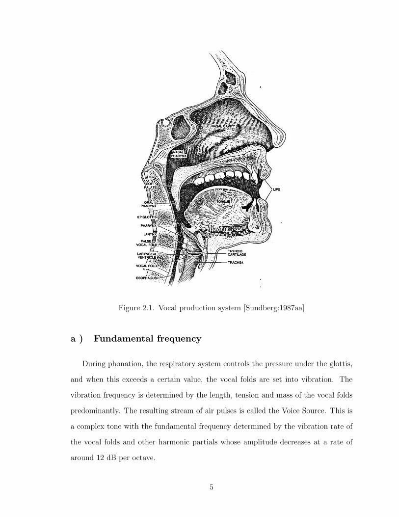
Figure 2.1. Vocal production system [Sundberg:1987aa]

a ) Fundamental frequency

During phonation, the respiratory system controls the pressure under the glottis,

and when this exceeds a certain value, the vocal folds are set into vibration. The

vibration frequency is determined by the length, tension and mass of the vocal folds

predominantly. The resulting stream of air pulses is called the Voice Source. This is

a complex tone with the fundamental frequency determined by the vibration rate of

the vocal folds and other harmonic partials whose amplitude decreases at a rate of

around 12 dB per octave.

5

b ) Formant frequencies

The vocal tract is a resonator and therefore the transmission of frequencies through

it is tied to its resonance frequency. Depending on the shape of the vocal tract, the

resonant frequencies vary. These frequencies are called formants, and they are the

least attenuated by the resonating tract, whereas for other frequencies of the vocal

folds, the attenuation is dependant on the distance from the resonant frequency.

These formants disrupt the smooth slope of the voice spectrum, imposing peaks on

the formant locations. The lowest formant corresponds to 14

ththe wavelength while

the second third and fourth formant correspond to 34

th, 5

4

thand 7

4

ththe wavelength

respectively. These four formants together form perturbations on the slope of the

voice spectrum to produce distinguishable sounds. Formants are characterized by

their frequency, amplitude and bandwidth.

The main determinants of the shape of the vocal tract are the jaw, the body of the

tongue and the tip of the tongue. Hence, any particular combination of these three

configurations can determine the set of the formant frequencies produced. Particular

combination of formants compose a vowel sound.

c ) Differences between singing and speech

Most work on analysis of the singing voice derives from the prior work on speech.

This requires an understanding of the differences between the two. In general, both

the intensity and frequency values as well as their ranges are narrower for speech than

for singing. The pitch dynamics in singing voice are piecewise constant with abrupt

pitch changes in contrast with the declination phenomenon in speech where the pitch

slowly drifts downwards with smooth pitch change in utternace. The effort from

the respiratory system is also usually lower for speech than singing. In singing, the

6

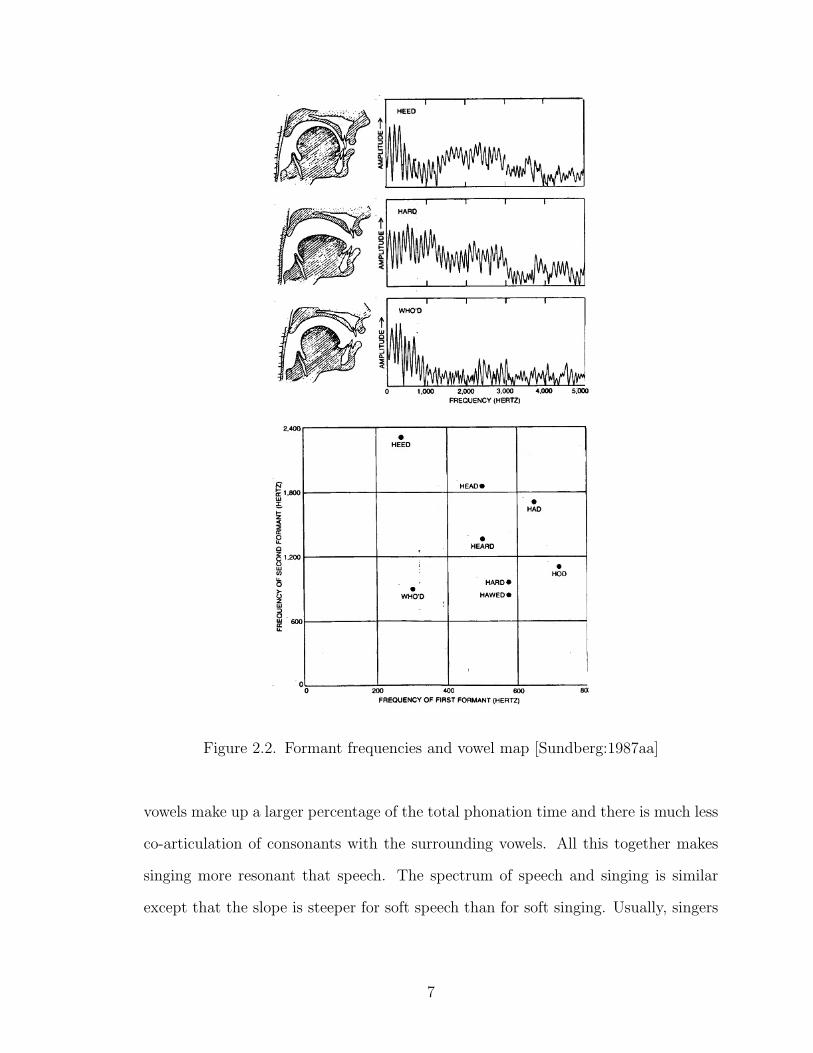
Figure 2.2. Formant frequencies and vowel map [Sundberg:1987aa]

vowels make up a larger percentage of the total phonation time and there is much less

co-articulation of consonants with the surrounding vowels. All this together makes

singing more resonant that speech. The spectrum of speech and singing is similar

except that the slope is steeper for soft speech than for soft singing. Usually, singers

7

adjust their vocal fold adduction to reduce the steepness of the spectral slope, giving

more energy to the higher partials.

The other major difference between a trained singer’s voice and speech is the

singing formant. This additional voal resonance while singing, which was deduced

by Sundberg [Sundberg:1987aa], is associated with lowering the larynx while singing.

This shift in larynx position is manifest as a lowering of the first two formants in

the spectrum of vowels. The lowering of the larynx, then, explains not only the

singing-formant peak but also major differences in the quality of vowels in speech

and in singing. Also, singers often raise the first formant frequency to be close to the

fundamental frequency of the pitch at which they are singing and this is seen in the

vowels’ spectra.

Figure 2.3. Singing formant [Sundberg:1987aa]

d ) Nasal voice production

Nasality is a type of resonant voice quality where the resonance occurs through

the nose. The nasal cavity does not have any muscles to adjust its shape, though it

is affected considerably by the swelling or shrinking of the mucous membrane. The

velum (a ap of tissue connected to the posterior end of the hard palate) can be raised

8

to prevent coupling between the oral and nasal cavity, or can drop to allow coupling

between them . When the lowering happens, the oral cavity is still the major source

of output, but the sound gets a distinctly nasal characteristic. The sounds which can

be nasalized are usually vowels, but it can also include semivowels, encompassing the

complete set of sonorant sounds.

Like the oral tract, the nasal tract has its own resonant frequencies or nasal

formants. House and Stevens [House:1956aa] found that as coupling to the nasal

cavity is introduced, the rst formant amplitude reduces, and its bandwidth and fre-

quency increase, and this was later confirmed by Fant [Fant:1960aa]. According to

Fujimura [Fujimura:1962kx] and Lieberman and Blumstein [Lieberman:1988yq] nasal

sounds present their main characteristic spectral properties in the 200 to 2500 Hz

range. Nasal consonants usually present their first formant at around 300 Hz and

their antiformant at around 600 Hz. Thus they concentrate energies in the lower

frequencies region and present little energy in the antiformant surroundings. Nasals

also present murmur resonant peaks, being the most significant at around 250 Hz

with a secondary minor peak at around 700 Hz.

The types of nasalization are as follows [Pruthi:2007rt]:

Coarticulatory nasalization

This occurs when nasals occur adjacent to vowels, and hence there is some opening

of the velopharyngeal port during atleast some part of the vowel adjacent to the

consonant, leading to nasalization of some part of the vowel.

9

Phonemic nasalization

Some vowels, though not in the immediate context of a nasal consonant are dis-

tinctively nasalized, as a feature of the word with a meaning different from the non

nasalized vowel.

Functional nasalization

Nasality is introduced because of defects in the functionality of the velopharyngeal

mechanism due to anatomical defects, central nervous system damage, or peripheral

nervous system damage.

2.2 Singing voice detection in music audio

The singing voice is the most representative and memorable element of a song,

and often carries the main melody, and the lyrics of the song. The problem of singing

voice detection is formulated thus given a segment of polyphonic music classify it

as being purely a mix of instrumental sources or one with vocals with or without

background instrumentation. This is the front end to applications like singer identi-

fication, singing voice separation, singing voice characterization, query by lyrics and

query by humming.

The features used for detection of singing voice can be grouped as follows [Ro-

camora:2007lq]

a ) Features used in speech

Some of the features extracted from the audio for the classification of a segment

into vocal or non vocal are derived from speech processing for speaker identifica-

10

tion and involve some representation of the spectral envelope. MFCCs and their

derivates, LPCs and their perceptual variant PLPs, and Warped Linear Coefficients

are examples of such features. They are not entirely satisfactory when characterizing

the singing voice in the presence of instrumental background.

b ) Features used in music content description systems

Some other features are borrowed from the audio content description realm,

mainly from research on instrument classification. Examples are

i. Since the voice is the most salient source, its usually accompanied by an increase

in energy of the frame.

ii. The singing voice is highly harmonic and so the harmonic coefficient can be used

to detect the singing voice. Also the number of harmonic partials present in the

frame increases when the voice is present, amidst an instrumental background.

iii. Spectral Flux, centroid and roll off are used in general instrument timbre iden-

tification and charcterization and can be applied to the singing voice.

iv. Perceptually motivated acoustic features like attack-decay contain information

about source.

v. The singing formant is a strong descriptor in some cases.

vi. Given the statistically longer vowel durations in singing, the vibrato is also a

good feature for singing voice detection [Nwe:2007pd], [Regnier:2009zr]. The

vibrato and tremolo both occur together in the singing voice unlike other in-

struments. Also the rate of the vibrato/tremolo and the extent are particular

to the singing voice.

11

These features are then classified using statistical classifiers such as GMM, HMM,

ANN, MLP or SVM. Frame based classifiers can cause over-segmentation with spu-

rious short segments classified wrongly. These are handled using post processing

methods like median filtering or using a HMM trained on segment duration. Fujihara

et al [Fujihara:2005bh] proposed a reliable frame selection method by introducting

two GMMs, one trained on features from vocal samples and another on non-vocal

sample features. Given a feature vector from a frame, the likelihoods are evaluated

for the two GMMs and based on a song dependent thresold the frames are classified

as reliable or not.

Recently, Peeters [Regnier:2009zr] proposed a simple system of threshold based

classification with only the tremolo and vibrato parameters from the audio signal as

descriptors. The performance of this method was comparable to a machine learning

approach with MFCCs and derivates as features and GMMs as statistical classifiers.

2.3 Singing voice isolation in music audio

Within a vocal segment, the voice is often present as a dominant source amidst

and instrumental background. So, to truly characterize the singing voice in terms of

timbre or melody or to extract lyrics from the signal, it is essential to identify and

extract the partials that belong to the voice. This is a vast and challenging field

of research and many different approaches have been attempted ranging from strict

source separation to simpler methods based on voice-specific features like vibrato and

tremolo.

The separation of speech has been extensively studied in contrast with singing

voice separation. The main difference between the signals in the context of separa-

tion techniques is the nature of concurrent sounds. In speech signals, the interference

12

is usually not correlated harmonically with the source. But in music, the accompani-

ment is harmonic and also correlated with the singing voice.

The separation techniques are dependent on the number of channels in the input

signal.

a ) Monoaural singing voice separation

For monoaural signals there has been much research based on fundamental fre-

quency estimation and partial selection based on a range of apriori information. Some

models of source separation are based on the auditory scene analysis process described

by Bregman [Bregman:1994aa] involving two stages segmentation and grouping. Such

approaches inspire researchers to build computational audio scene analysis systems

which perform sound separation with minimal assumptions about concurrent sources.

Some cues used for CASA systems are common onset and common variation as well

as pitch cues or the harmonicity principle. In a recent paper Peeters [Regnier:2009zr]

separate out the singing voice partials based on partial tracking and the presence of

vibrato and tremolo modulations in the partials.

b ) Stereo audio singing voice separation

For a stereo signal, the separation of the singing voice can make use of the pres-

ence of phase and panning information. This is in line with the spatial location cue

of grouping in the Auditory Scene Analysis approach. One approach of note is pro-

posed by Vinyes et al. [Vinyes:2006mz] where the separation is attempted based on

extraction of audio signals that are perceived similarly to the audio tracks used to

produce the mix using a mixture of panning, phase difference and frequency range

input specified by a human user. In popular recordings, its often the case that the

13

voice is recorded on a mono track and panned to the center of the stereo recording.

Operating on this assumption it is possible to obtain a voice track from the stereo

polyphonic music signal using pre-determined phase, frequency and panning value

ranges.

2.4 Nasality description in speech

The first comprehensive research into characterising nasality was done by Fant

[Fant:1960aa]. Speakers with a defective velopharyngeal mechanism produce speech

with inappropriate nasal resonance. Clinical techniques exist to detect such hyper-

nasality, but are usually invasive and hence lead to artificial speaking situations. A

preferred approach would be non invasive and could be based on signal processing

and estimation of nasality. The acoustic cues for nasalization include

i. First formant bandwidth increases and intensity decreases.

ii. Nasal formants appear.

iii. Antiresonances appear.

a ) Spectral differences between nasal and non-nasal singing

The spectra of the same piece of music sung by the same person, first nasally and

non nasally would provide a good comparison of the differences between nasal and

non-nasal voice production. This task has already been performed by Sotiropoulos

[Garnier:2007aa]. This study included recordings from professional bass baritone

singers singing the same piece first normally, and then in a nasal mode. The spectra

of these renditions are shown below, first normal and then nasal :

14

Figure 2.4. Spectrum of normal singing

Figure 2.5. Spectrum of nasal singing

From these spectra, it is clear that the nasal signal contains several additional

peaks above the 2500Hz region, when compared with the normal voice. Also, the

energy around the 1000Hz region is higher for nasal sounds. This spectral be-

haviour is also seen in higher pitched vocal melodies and is pitch independent [JJen-

nings:2008aa].

Some of the approaches to nasality detection are listed below.

15

b ) Teager energy operator based detection

Cairns et al. [Cairns:1996gf] proposed detecting hypernasality using a measure of

the difference in the non linear Teager Energy operator profiles.

Normal speech is expressed as a sum of formants Fi, i = 1, 2, ...Iat various fre-

quencies. Nasal speech includes nasal formants NFi, i = 1, 2, ...M and antiformants

AFi, i = 1, 2, ...K.

Snormal =I∑i=1

Fi(w) (2.1a)

Snasal =I∑i=1

Fi(w)−K∑k=1

AFk(w) +M∑m=1

NFm(w) (2.1b)

Since primary cue for nasality is the intensity reduction of the first formant F1,

the equations can be simplified with a Low Pass Filter

Snormal−LPF = F1(w) (2.2a)

Snasal−LPF = F1(w)−K∑k=1

AFk(w) +M∑m=1

NFm(w) (2.2b)

The multicomponent for the nasal speech vector can be exploited using the non

linearity of the Teager Energy Operator , which is defined over x(n) as

ψd[x(n)] = x2(n)− x(n− 1).x(n+ 1) (2.3)

Applying TEO to the low pass filtered nasal and non nasal speech, results in

ψd[Snormal−LPF (n)] = ψd[fI(n)] (2.4a)

16

ψd[Snasal−LPF (n)] = ψd[fI(n)]−K∑k=1

ψd[AFk(n)] +M∑m=1

ψd[NFm(n)] +K+M+I∑j=1

ψcross[]

(2.4b)

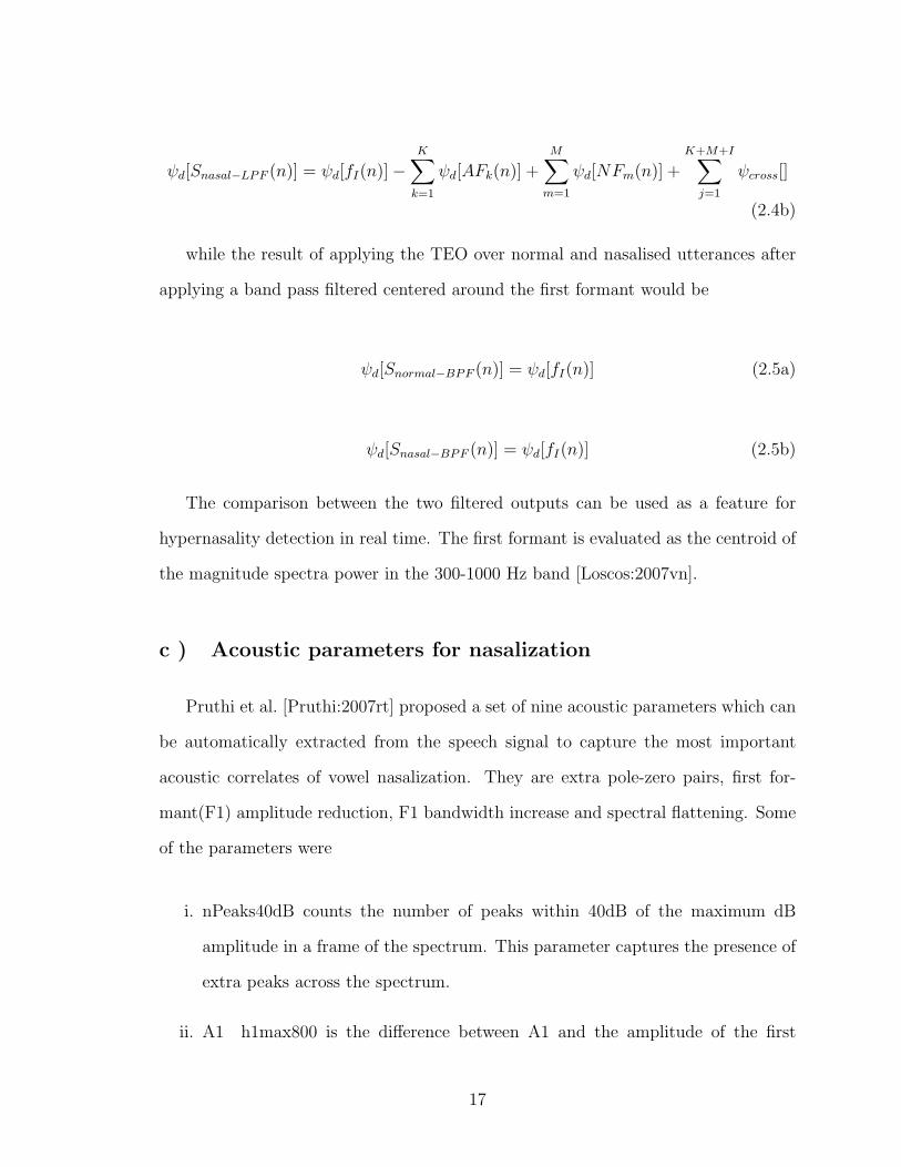
while the result of applying the TEO over normal and nasalised utterances after

applying a band pass filtered centered around the first formant would be

ψd[Snormal−BPF (n)] = ψd[fI(n)] (2.5a)

ψd[Snasal−BPF (n)] = ψd[fI(n)] (2.5b)

The comparison between the two filtered outputs can be used as a feature for

hypernasality detection in real time. The first formant is evaluated as the centroid of

the magnitude spectra power in the 300-1000 Hz band [Loscos:2007vn].

c ) Acoustic parameters for nasalization

Pruthi et al. [Pruthi:2007rt] proposed a set of nine acoustic parameters which can

be automatically extracted from the speech signal to capture the most important

acoustic correlates of vowel nasalization. They are extra pole-zero pairs, first for-

mant(F1) amplitude reduction, F1 bandwidth increase and spectral flattening. Some

of the parameters were

i. nPeaks40dB counts the number of peaks within 40dB of the maximum dB

amplitude in a frame of the spectrum. This parameter captures the presence of

extra peaks across the spectrum.

ii. A1 h1max800 is the difference between A1 and the amplitude of the first

17

harmonic H1. The value of A1 was estimated by using the maximum value in

0-800Hz. This captures the reduction in F1 amplitude.

iii. std0-1K is the standard deviation around the center of mass in 0-1000Hz. This

parameter not only captures the spectral flatness in 0-1Khz but also captures

the effects of increase in F1 bandwidth and reduction in F1 ampltide.

The best performance among these parameters were found for std0-1Khz. The

results using the nine suggested parameters was comparable to that of using Mel

Frequency Cepstral coefficients and their delta and double delta values (MFCC +

DMFCC + DDMFCCs).

2.5 Discussion

This chapter contained a review of the previous research related to the different

aspects of singing voice description, isolation and nasality characterization. There

are some limitations to each of the approaches discussed. The isolation of the voice

partials is the most challenging aspect of the process when dealing with polyphonic

music. Hence, the accepted compromise is to assume that if the voice is the predom-

inant source in the frame, the spectral envelope will be most representative of the

voice spectrum and hence a partial accompaniment reduction will provide acceptable

results. The main concern in this thesis is to characterise the voice in terms of nasal-

ity. This has been dealt with extensively in speech, but there has not been much work

on identifying nasality in the singing voice, especially in polyphonic music. Hence the

main contribution in this thesis is that of identifying strong descriptors for nasality in

the singing voice segment, while some instrumental background is still present. Also,

much of the singing voice isolation has been made with monoaural recordings, and

18

using the panning information for identifying the perceptually relevant voice track is

a contribution of this work.

19

Chapter 3

Selected Approach

This chapter discusses the steps selected for the nasality detection.

3.1 Music material

The music material used for this analysis is selected from commercial recordings

of popular music, from country, rock and pop music. An existing dataset for western

popular music is the CAL500 dataset [Turnbull:2008ul] containing 500 songs tagged

with 22 tags for the singing voice among other semantic musically relevant tags.

These 22 tags are

Aggressive, Altered with Effects, Nasal, Breathy, Off-key, Call & Response, Duet,

Scatting, Emotional, Falsetto, Gravely, High-pitched, Low-pitched, Monotone, Rap-

ping, Screaming, Spoken, Strong, Unintelligible, Virtuoso, Vocal Harmonies, Weak

Some statistics regarding the occurrence of these tags might give one an idea of

their prevalance. The tag for Harmonies are present on all song and 50% of the songs

20

are tagged as Emotional. Roughly 25% of the songs are tagged as High-pitched and

22% as low-pitched. The nasal tag is present on 10% of the songs.

One of the sources of ground truth for music tagged as nasal is the last.fm

[Last.fm:aa] database of tags. For a search involving artists tagged as nasal, the

results include 62 artists. The other source of ground truth is the wikipedia article

on the nasal voice [Wikipedia:aa] where the list of artists overlaps with those from

last.fm with a few distinct names.

As there are no other databases which contain a large collection of commercial

popular music recordings with tags for the nasal voice, the music material for this

thesis has been compiled out of my personal collection, with songs representative of

each of the artists listed as nasal in the above sources of ground truth. The selection

has been restricted to pop, rock and country music, and contains 70 songs with 3

songs from each artist. The male and female singers are equally represented and the

voices and instrumentation are thought to equally represent a range of voices and

instrumentations within the pop-rock genre.

The ground truth for non-nasal voices is even more difficult to obtain, since the

definition of such a voice is in itself not concrete. So the set of samples representative

of the non-nasal class has been compiled based on personal discretion. Some features

of the selected dataset are :

90 songs collected from 28 artists (Appendix A)

43 songs contain female voices and 47 male.

Each song segment is approximately 30s in length

60% of the songs are from the Pop genre and the rest are from the country, rock

and jazz genres.

21

3.2 Preprocessing (isolation)

Once the data is collected, the vocal segments need to be selected. For our ap-

proach, the choice of segment with predominant vocals is done manually, with the

segment length of approximately 30s, with the voice present as continuously as pos-

sible through the segment.

Each of these stereo segments is converted to .wav, with a sampling rate of

44100Hz. The next step is to convert the stereo segments into mono for further

processing. This can be done by a simple averaging of the left and right channels.

However, some pre-processing can also be performed with the stereo information to

achieve accompaniment sound reduction.

The following manipulations are performed on the audio tracks to obtain a mono

track with boosted vocals. Firstly, the signal spectrogram is generated, with a window

size of 8192 samples and a hop size of one fourth the window length.

a ) Frequency filtering

The vocals in popular music can be found within the 200 to 5000 Hz range, and

band-pass filtering the signal to this frequency range should eliminate some of the

bass and drums as well as the instruments in the higher frequency ranges.

The filtering is performed directly on the frequency spectrum of the signal by

setting the values of the outlying bins to zero.

b ) Phase difference based filtering

Assuming that the voice source is originally recorded as a mono track and mirrored

on both tracks, to be at the center of the mix, implies that the phase is the same for

22

the spectral components of the voice on both channels. This allows us to filter the

tracks based on inter-channel phaqse difference, selecting only the components which

have near zero values.

Thus if the extracted sound is the original voice track, the phase difference between

the left and right components would be zero,

|Arg(DFTp(sLi )[f ])− Arg(DFTp(s

Ri )[f ])| = 0 ∀ f ε 0...N/2 (3.1)

whereas for mono tracks with artificial stereo reverberation or stereo source tracks,

the phase difference will be greater than zero, as in the following case

|Arg(DFTp(sLi )[f ])− Arg(DFTp(s

Ri )[f ])| > 0 ∀ f ε 0...N/2 (3.2)

To allow for a small margin for the phase difference, the choice of difference values

is set at -0.2 to 0.2.

It may happen that the track has not only the mirrored DFT coefficients, but also

some with differing phases, in which case some dereverberation is performed. Since

we are interested in the vocal quality of the mono voice signal, this is an advantage.

c ) Panning ratio based filtering

In general when a mono track is set at a particular location in the stereo mix, a

panning coefficient is applied which would help decide whenther a sound may corre-

23

spond to a track or not. Consider ini[k], the original mono tracks of the mixture,

which is mixed as

inLi [k]

inRi [k]

=

αLi .ini[k]

αRi .ini[k]

(3.3)

In general, most analog and digital mixtures follow the following pan law based

on the angle at which the track is present in the stereo space. Here x ε [0, 1]

αLi = cos(x.π

2) =

√1

1+(αRi +αL

i )2

αRi = sin(x.π2) =

√(αR

i +αLi )2

1+(αRi +αL

i )2

x = arctan(αR

i

αLi

). 2π

(3.4)

Hence if the extracted sound sLi [k], sLi [k] is one of the original stereo tracks, it will

verify

sRi [k]

sLi [k]=inRi [k]

inLi [k]=αRiαLi

= constant (3.5)

Since DFT is a linear transformation, this relationship is also maintained in the

coefficients and therefore,

DFTp(sRi )[f ]

DFTp(sLi )[f ]= constant ∀ f ε 0...

N

2if DFTp(s

Ri )[f ] 6= 0 or DFTp(s

Li )[f ] 6= 0

(3.6)

For the voice signal which is supposed to be panned to the center of the mix, the

panning coefficient should be around 0.5, and to allow for some margin, the range of

values chosen is from 0.4 to 0.6.

24

The zero phase difference rule can be used as a prior step to the panning ratio,

because the latter presupposes that the same sound is present in both channels.

At the end of this pre-processing step, the resulting spectrogram of a single track

signal can be used directly for spectral feature extraction. Additionally, the spectro-

gram is also re-synthesized with overlap-add to regenerate the wave file which can be

used for some features like the Teager Energy operator.

3.3 Feature extraction

The output of the mono conversion module is a spectrogram with window length

of 8192 and hop size of 1/4th the window size.

This is used frame by frame for the descriptor extraction module. The following

steps are performed:

a ) Discarding frames unsuitable for feature extraction

Discard percussive frames

Attempt to identify percussive frames using the following code [Aucou-

turier:2004aa],

spectralflatness =(∏

(spec))1N

1N

∑spec

normalizationfactor = max(spec)−min(spec);

σ3 = 3var(spec)

normfactor

25

If Spectral Flatness > σ3, it is a percussive frame and is hence discarded.

Discard silent frames

Silent frames are discarded, with the criterion of the maximum dB level of the

frame being less than −60, empirically.

Discard inharmonic frames

The effect of nasality is present mainly in the vowels and hence the inharmonic

frames can be discarded before feature extraction. SMS based Harmonic analysis

is performed on the frame to identify if it is a harmonic source and also to obtain

the pitch estimate. The parameters for the harmonic analysis are as follows, set

empirically based on the most often present values for the fundamental frequency

and the deviations from the value in the music audio samples.

Minimum f0 = 150

Maximum f0 = 600

Error threshold = 2

Maximum harmonic deviation = 14

Energy and kurtosis around 2.5KHz

The energy in the 2.5Khz region(2400-2600Hz) is lower for nasal sounds because

of the nasal anti-resonance that gets added in this region. The kurtosis measure is

used as an attempt to capture the dip of the spectrum in this region.

26

Energy and kurtosis around 4KHz

The energy in the 4Khz region(3900-4100Hz) is higher for nasal sounds from the

spectrograms of acapella sounds that were analyzed. The kurtosis measure is used as

an attempt to capture the peak of the spectrum in this region.

b ) Spectral peaks based descriptors

std0-1KHz

The standard deviation around the center of mass in the 0-1000 Hz region, ac-

cording to [Pruthi:2007rt], captures the spectral flattening at the low frequencies, as

well as the increase in F1(first formant) bandwith and reduction in F1 amplitude.

This value is higher for nasal sounds as compared to normal voices.

nPeaks40dB

The number of peaks within 40dB of the maximum is expected to be higher for

nasal voices due to the assymetry of nasal passages and coupling to the nasal cavity

that causes additional pole zero pairs to appears all through the spectrum.

c ) Features based on formants

a1-h1max800

The difference between the amplitude of the first formant(A1) and the amplitude

of the rst harmonic (H1) is a descriptor capturing the weakening of the first formant.

The value of A1 was estimated by using the maximum value in 0-800 Hz. This should

27

be lower for nasal sounds since there is a flattening at the lower frequencies for nasal

sounds

Teager energy operator comparison

The Teager Energy operator descriptor is based on the comparison of the low pass

filtered and band pass filtered signal, which allows for nasality detection in the voice.

Once these descriptors have been computed for each frame, they can be used

by averaging them for the entire sequence or by other transformations. The method

chosen here is to first view the descriptor distributions for nasal and non nasal samples

and then choose thresholding values for the descriptors that could potentially imply

a separation in class.Then, the count of frames which satisfy the threshold can be

used as the feature vector input to the classifier.

3.4 Classification

The classification of the singing voice as being nasal or non-nasal is essentially a

two class classification problem. However, since the characterization of non-nasality

is not well defined, the outlier space is not as well sampled as that of the target. So it

needs to be formulated as a one-class classification problem, where the target is well

represented whereas the outliers are sparsely populated.

This does not necessarily mean that the sampling of the target class training set

is done completely according to the target distribution found in practice. It might be

that the user sampled the target class according to his/her idea of how representative

these objects are. It is assumed though, that the training data reflect the area that

the target data covers in the feature space.

The outlier class can be sampled very sparsely, or can be totally absent. It might

28

be that this class is very hard to measure, or it might be very expensive to do the

measurements on these types of objects. In principle, a one-class classifier should be

able to work, solely on the basis of target examples. Another extreme case is also

possible, when the outliers are so abundant that a good sampling of the outliers is

not possible. This is the case with the tag of non-nasality.

a ) Training and model selection

The DD Tools Matlab toolbox [Tax:2009aa] contains several classifiers, tools and

evaluation functions for data description and one class classification. All classifiers

in this toolset have a false negative as an input parameter, and by varying this value

and measuring the error on the outliers accepted, the ROC can be found.

The data is labelled target and outlier and prepared in the format expected by

the toolbox. This is then sent through a 10 fold cross-validation cycle, where the

data split into 10 folds with 9 used for training at a time, and 1 for testing. The FN

fraction is set to 0.2 and more than one classifier is used for training. Among the

cycles, the model which performs the best is chosen for final training of the complete

dataset. The criterion for choice are that the False Negative and False Positive ratios

are below a particular threshold, and amongst the cycles for which this is satisfied,

the iteration with the best value of Area under Curve is chosen. This AUC calculation

is done within the boundary of [0.1 to 0.67] since the outlier acceptance rate of more

than 2/3rd is considered unacceptable. This provides a more reliable estimate of the

performance of the classifier.

29

Figure 3.1. ROC with AUC Boundary

b ) Alternative classifiers

The general classifiers found in the WEKA tool [Witten:2005aa] are also used to

evaluate the performance of the descriptors chosen in the preceding sections. The

chosen model is that of a tree based classifier with boosting incorporated called the

Alternating Decision Tree(ADTree) [Freund:1999aa]. The advantage of such boost-

ing algorithms is that they combine several weak rules to form a stronger one, for

classification and hence are somewhat robust to outliers. The ADTree can also be

used to identify the strength of information gain for each of the descriptors as each

descriptor is thresholded and contributes to the overall evaluation proportionally to

its rank. The attribute ranking can also be evaluated using the attributeSelection

function in WEKA.

30

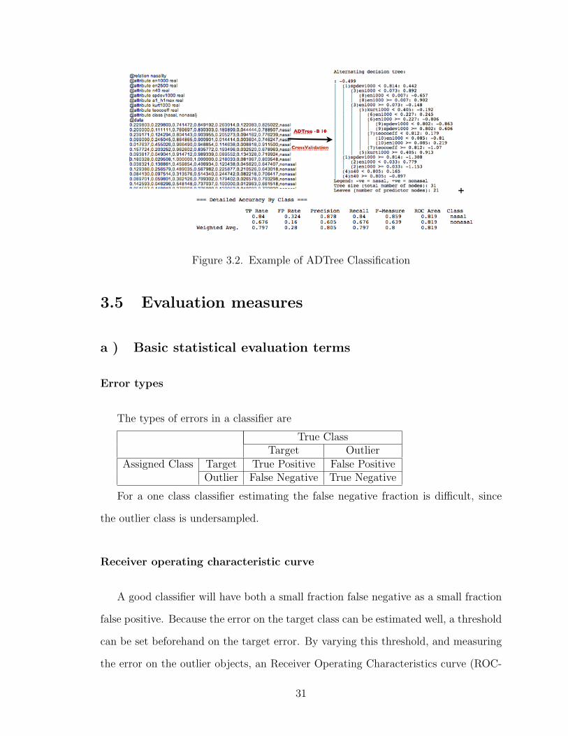
Figure 3.2. Example of ADTree Classification

3.5 Evaluation measures

a ) Basic statistical evaluation terms

Error types

The types of errors in a classifier are

True ClassTarget Outlier

Assigned Class Target True Positive False PositiveOutlier False Negative True Negative

For a one class classifier estimating the false negative fraction is difficult, since

the outlier class is undersampled.

Receiver operating characteristic curve

A good classifier will have both a small fraction false negative as a small fraction

false positive. Because the error on the target class can be estimated well, a threshold

can be set beforehand on the target error. By varying this threshold, and measuring

the error on the outlier objects, an Receiver Operating Characteristics curve (ROC-

31

curve) is obtained. This curve shows how the fraction false positive varies for varying

fraction false negative. The smaller these fractions are, the more this one-class clas-

sifier is to be preferred. Traditionally the fraction true positive is plotted versus the

fraction false positive, as shown

For comparison purposes, an Area Under Curve(AUC) parameter is defined for

an ROC curve which is the integral of the false positive fraction over the range of

thresholds from 0 to 1. Smaller values indicate a better separation between targets

and outliers.

Precision, recall and F1 measure

These are often-used measures defined as follows :

Precision :

precision =# of correct target predictions

# of target predictions(3.7)

Recall :

recall =# of correct target predictions

# of target examples(3.8)

F1 :

F1 =2 . precision . recall

precision + recall(3.9)

32

b ) Cross validation

In cross validation, the dataset is split into N batches and from these N-1 are

used for training and 1 for testing, and the performance is averaged over the N

repetitions. This has the advantage that given a limited training set it is still possible

to obtain a good classifier and to estimate its performance on an independent set.

The repetition of the cross-validation procedure also helps finetune the parameters

and to aid selection of the best model.

33

Chapter 4

Results

This section presents the outcomes of the steps elaborated in the previous chapter.

The procedure was extended to include a comparison with some more standard feature

vectors composed of MFCC values and some low level spectral descriptors described

in [Peeters:2004aa].

The configuration with the descriptors developed especially for nasality and de-

scribed in the preceding sections is titled ’conf1’ and that with the the generic feature

set is titled ’generic’.

4.1 Feature vector

The database for evaluation consists of 94 songs from 27 nasal artists and 32 non

nasal songs. A sample of each class is presented here.

Nasal

Non-nasal

34

a ) Nasality specific feature vector

The selected descriptors for conf1 are

i. en1000 - Energy around 1KHz

ii. en2500 - Energy around 2.5KHz

iii. n40 - Number of Peaks within 40dB of the maximum

iv. spdev1000 - Spectral deviation in the 1KHz region

v. a1-h1max - Difference between the first formant amplitude and the first har-

monic amplitude

vi. kurt100 - Spectral Kurtosis around the 1KHz region

vii. teocoeff - Nasality coefficient based on Teager Energy Operator comparison

35

(a) Nasal - en1000 (b) Non nasal - en1000 (c) Nasal - nPeaks40dB

(d) Non nasal - nPeaks40dB (e) Nasal - spdev1KHz (f) Non nasal - spdev1KHz

(g) Nasal - a1h1max800 (h) Non nasal - a1h1max800 (i) Nasal - kurt1000

(j) Non nasal - kurt1000

Figure 4.1. Extracted features for Conf1

36

As is clear from the plots, the values of en1000, kurt1000, nPeaks40dB and

spdev1KHz are higher for the nasal sample than for the non-nasal sample on an

average. This is as expected from the definition of the features.

b ) Generic feature vector

The selected descriptors for this configuration ’generic’ are

i. MFCC 0-12 - MFCC coefficients

ii. Spectral Centroid

iii. Spectral Energy:Band-Low

iv. Spectral Energy:Band-Middle High

v. Spectral Energy:Band-Middle Low

vi. Spectral Flatness

vii. Spectral Rolloff

viii. Spectral Strong Peak

ix. Odd to Even Harmonic Energy Ratio

The Spectral Centroid was expected to be higher for the nasal sounds since the

spectrum was flatter and thus like noisy signals, the centroid would become higher

The Spectral Energy in the bands Low, Middle-Low and Middle-High were chosen to

capture the dips and peaks in the spectrum introduced by the nasal resonances. The

Spectral Flatness as mentioned before, was predicted to be higher and the Roll off

less steep. The spectral strong peak was expected to be less for nasal sounds and the

37

Odd to Even Harmonic Energy ratio was chosen because it is known to be relevant

to nasal sounding instruments.

These descriptors together form a 21 length feature vector under the configuration

generic.

c ) Pre-processing configurations

The results were evaluated for the three sets of preprocessed data

i. Simple Mono - Mono

ii. Frequency filtered Mono - Freq

iii. Frequency, Phase Difference - FrPh

iv. Frequency, Phase Difference and Panning ratio range filtered Mono - FrPhPn

The results of the different pre-processing methods are represented by the samples

presented here.

Simple mono

Frequency filtered

Frequency and phase filtered

Frequency phase and pan filtered

d ) Visualizing the Descriptors

The feature vectors were written in arff format and uploaded on Weka to view the

distribution of the values for each for the different configurations and pre-processing

styles.

38

(a) Conf1 - Mono (b) Conf1 - Freq

(c) Conf1 - FrPh (d) Conf1 - FrPhPn

Figure 4.2. Feature Distribution for Conf1

39

(a) Generic - Mono (b) Generic - Freq

(c) Generic - FrPh (d) Generic - FrPhPn

Figure 4.3. Feature Distribution for Generic

40

4.2 Attribute Significance

Using attribute selection with Information Gain ratio evaluation, with 10 fold

cross validation

Average Merit Average Rank Attribute0.17 +- 0.015 1 +- 0 n40

0 +- 0 2.6 +- 1.02 en10000 +- 0 3.2 +- 0.4 en25000 +- 0 4.8 +- 1.25 kurt1000

0.019 +- 0.038 5.2 +- 1.6 spdev10000 +- 0 5.3 +- 0.64 teocoeff

0.021 +- 0.042 5.9 +- 1.81 a1-h1max

Table 4.1. Attribute Ranking - Conf1

From the above table it is clear that n40 is the most relevant attribute followed

by en1000 and en2500. The Teager Energy Coefficient and a1-h1max do not seem

to offer much of an information gain, however removing these terms does diminish

outlier detection. These facts can also be visually verified by observing the graphs

plotting the descriptor distributions.

For generic descriptors, the gain ranking changed considerably for the different

pre-processing configurations. However there were some constant trends indicating

that the three main information providers were mfc0, mfc6 and spectral flatness in db.

Spectral energy in the midde-high band is also a reasonably high ranked descriptor.

No trend could be discovered in the other descriptor relevances.

41

Average Merit Average Rank Attribute0.192 +- 0.008 1.6 +- 0.49 mfc00.169 +- 0.014 2.7 +- 0.46 spectral flatness db0.132 +- 0.015 3.6 +- 0.8 spectral energyband middle high0.113 +- 0.011 5.4 +- 0.66 spectral rolloff0.102 +- 0.036 5.8 +- 1.47 mfc20.067 +- 0.055 6.5 +- 1.43 mfc60.134 +- 0.11 6.6 +- 6.86 oddtoevenharmonicenergyratio

0 +- 0 8.4 +- 0.8 mfc70 +- 0 9.6 +- 1.85 mfc50 +- 0 9.7 +- 0.9 mfc10 +- 0 10.5 +- 1.5 mfc30 +- 0 11.7 +- 0.46 mfc4

0.021 +- 0.043 13.3 +- 6.02 mfc80 +- 0 13.5 +- 0.5 spectral energyband low0 +- 0 14.9 +- 1.58 spectral energyband middle low

0.01 +- 0.029 15.4 +- 3.41 spectral centroid0 +- 0 15.5 +- 0.5 spectral strongpeak0 +- 0 17.5 +- 0.5 mfc90 +- 0 18.9 +- 1.58 mfc100 +- 0 19.4 +- 1.74 mfc120 +- 0 20.5 +- 0.5 mfc11

Table 4.2. Attribute Ranking - Generic

4.3 Classification results

The following classifiers were chosen to train, obtain a model for and the eval-

uate the results thereof. Density and reconstruction methods are both chosen for

evaluation.

i. Gaussian

ii. Parzen Density

iii. Self Organising Maps

iv. Support Vector

v. Principal Component Analysis

42

vi. KMeans

The method was to perform 10-fold cross validation on the data set for each

classifier, discard all runs that involved a false positive(FP) rate greater than .67 and

a true positive(TP) rate less than .5. Of the valid runs past this step, the one with

the best Area under the curve(AUC) value was selected for training the final data set

and testing it. AUC was calculated between the error boundaries of 0.1 and 0.6 to

be more representative of the region of outlier acceptance we were willing to tolerate.

This ensured a better comparison of actual classifier performance.

The overall results for the one-class classifier trained with the seven descriptors

listed above are as follows

43

Mono Frequency Freq-Phase Freq-Phase-Panconf1 generic conf1 generic conf1 generic conf1 generic

FNkmeans 0.1064 0.8298 0.1 0.7158 0.0857 0.2979 0.0857 0.0851

pca 0.0851 0.883 0.0857 0.5532 0.1 0.1383 0.0857 0.0957som 0.0957 0 0.0426 0.3617 0 0.0851svdd 0.1383 0.0957 0.5106 0.3511

parzen 0.1064 0.5 0.0851

FPkmeans 0.6176 0.2353 0.7143 0.2353 0.7619 .6765 0.619 0.8235

pca 0.7941 0.3235 0.7143 0.4118 0.7143 0.9118 0.7619 0.9412som 0.4118 0.5882 0.6471 0.7059 0.7059 0.7941svdd 0.8235 0.7353 0.5294 0.6471

parzen 0.1471 0.6471 0.8235

Precisionkmeans 0.8 0.6667 0.8077 0.7714 0.8 0.7416 0.8312 0.7544

pca 0.7611 0.5 0.8101 0.75 0.8077 0.7232 0.8 0.7265som 0.8586 0.8246 0.8036 0.7143 0.7966 0.7611svdd 0.7282 0.7596 0.7188 0.7349

parzen 0.9438 0.6812 0.7544

Recallkmeans 0.8936 0.1702 0.9 0.2872 0.9143 0.7021 0.9143 0.9149

pca 0.9149 0.117 0.9143 0.4468 0.9 0.8617 0.9143 0.9043som 0.9043 1 0.9574 0.6383 1 0.9149svdd 0.7979 0.8404 0.4894 0.6489

parzen 0.8936 0.5 0.9149

AUCkmeans 0.70257 0.70087 0.68756 0.35979 0.38365 0.36857 0.43724 0.42091

pca 0.52718 0.67012 0.54963 0.59602 0.3998 0.4328 0.48957 0.4613som 0.87915 0.92952 0.88224 0.264 0.84576 0.64585svdd 0.39983 0.49208 0.38113 0.41762

parzen 0.99638 0.86414 0.48758 0.41955

Table 4.3. One Class Classifiers Evaluation

44

SOM performs very well for some configurations and SVdd for others. The

gaussian-based density estimators were uniformly poor at outlier detection rate, ac-

cepting outliers at a ratio greater than .8.

a ) Error Analysis

The erroneous instances were analysed and the following patters were found. For

false negative cases, the following were the causes :

i. In some cases the assumption of mono, center-panned solo vocal track is not

valid and in these cases, the output of the frequency, phase and pan filtered

mono conversion module is unsuitable for further processing. These tracks then

lead to false negatives when classified.

ii. Some of the instances of false negatives occurred when the extracted mono track

included drum sounds. This is because the percussive sounds add several peaks

to the spectrum and hence skew the extracted features.

iii. When the voice was not continuous and the extracted track contained silent

portions, the feature values were such that false negatives occurred.

For false positives, one of the causes is the low quality of extracted mono track.

But for many cases, no such pattern is found. The preference for lower false negatives

in the training process is likely to be the reason for these outliers being accepted.

4.4 Summary of Results

The overall results were such that with generic datasets, the false positive(FP)

and false negative(FN) rates were never both within acceptable range, and it showed

consistently worse separation between the target and outlier.

45

The best results were found for the Conf1 configuration for Freq only pre-

processing where all the models showed good precision and recall ratios and high

area under the curve(AUC) values.

For evaluation of vocal separation techniques, the best results were observed for

the highlighted case of Conf1 with Fr-Ph (FP = 0.64, FN = 0.04, AUC = 0.88).

This occured with the SOM classifier. An equivalent can be found in Conf1 with

Fr-Ph-Pn with Kmeans classifier, though the AUC is lower than desired. (FP =

0.62, FN = 0.08, AUC = 0.44)

It was expected that the pre-processing with center track extraction would pro-

vide better results than other methods. However, the simple frequency filtering has

provided the best results so far. This may be explained by the fact that many of the

descriptors depend on the spectral spread and number of peaks, and the vocal track

has fewer spectral peaks. However, the fact that even the lower values of accuracy are

near .6 should indicate that the descriptors are valid. Also, in some cases the center

track preprocessing resulted in bad audio tracks due to some fault in the assumption

of mono track - center panning, or due to the selected range of parameters. This also

needs to be investigated.

46

Chapter 5

Conclusion

In this final chapter of the thesis, a summary of the task undertaken is presented

along with some reflections and conclusions as well as suggestions for future work on

the topic for improved understanding and implementation.

5.1 Summary of contributions

The goals of this thesis as stated in the Introduction (1.2) were :

To obtain a small set of carefully chosen descriptors to provide a reliable nasal

measure.

To evaluate the efficacy of stereo information based accompaniment reduction

for vocal separation

The first step of performing a comprehensive study of the state of the art led

to the confirmation of the fact that nasality in the singing voice has not been used

extensively so far in MIR systems, though it has been much researched in speech under

the applications of detection and correction of hypernasality as well as for language

47

specific phoneme and semantic recognition. Once the need for work in this area was

established, the descriptors and knowledge base from speech signal processing were

evaluated in the context of the singing voice. It was found that since nasality was a

resonant phenomenon, and the singing voice contained a higher ratio of vowel sounds

which contribute to harmonic structure, the descriptors pertaining to the harmonic

peaks as well as the formant locations could be used in the singing voice too. This

conclusion was further bolstered by the analysis of several solo singing voice spectra,

for nasal and non nasal renditions, which confirmed the earlier hypothesis.

The specific circumstance of working with real recorded music meant that the

vocal track was not present as a solo source, and some stereo-information based

filtering techniques were adopted from [Vinyes:2006mz] to extract the singing voice

from the polyphonic data. To evaluate the performance of this method of filtering

as opposed to unfiltered signals, several combinations of datasets were formed [4.1].

These were then evaluated using several classifiers [4.3].

The Stereo information filtering techniques did not work as well as the simple

Frequency filtering technique, though some explanation of that may lie in the fact

that the descriptors were heavily dependent on number of spectral peaks present.

The overall results however confirmed the fact that the outlier acceptance rate could

be kept low without affecting the False Negative rate. This indicates that the chosen

descriptors do provide a good separation between the nasal and non nasal signals.

The chosen descriptor set was also compared against a generic descriptor set

composed of MFCCs and some low level spectral descriptors [ 4.1]. This showed

that while the generic descriptor set did not provide as robust a target and outlier

separation as the chosen descriptors. The best performance for the generic descriptor

set was that of the Frequency-PCA configuration where the FP rate was .41 while

the FN rate was .55. This is a distant second to the best performance with the chosen

48

descriptors which was an FN rate of 0.5882 with no target error resulting in an AUC

of .93.

5.2 Plans for future research

The phenomenon of nasality in speech is one with several dimensions, and in our

thesis only a general idea of nasality has been considered. For example, the nasality

can occur due to the predominance of nasal elements and inflections in the language,

due to the constriction of the ridge of the nose, due to actual hyper-nasal conditions

etc. It is possible for artists with a normal voice to sound nasal in particular passages

of music, intentionally. These distinctions have not been captured and some study is

needed into the particular aspects of nasality as applied to the singing voice.

The one-class classification has been performed with a set of classifiers represen-

tative of different data description methods. No attempt has been made to match

the structure or behaviour of the descriptors to the biases and characteristics of the

classifiers. It is possible that some transformation of data in the feature set would

result in more information gain thence leading to better classification.

The stereo information based filtering has not shown the performance improve-

ment that had been expected at the beginning of the thesis, because of the dependence

of features on spectral peak data, possibly. This can be considered a drawback, and

some study into making the descriptors more robust to other sources surrounding the

voice would be very useful in the context of MIR systems. On the other hand, a robust

method of voice track separation would eliminate other sources from the recording

even before the descriptors are calculated making them more representative of the

voice signal.

49

References

[Sundberg:1987aa] J. Sundberg, The Science of the Singing Voice. Northern Illinois University

Press, 1987.

[Grey:1977aa] J. M. Grey, “Multidimensional perceptual scaling of musical timbres,” The Journal

of the Acoustical Society of America, vol. 61, no. 5, pp. 1270–1277, 1977.

[Rusko:1997aa] M. Rusko, “Towards a more general understanding of the nasality phenomenon,” in

Music, Gestalt, and Computing - Studies in Cognitive and Systematic Musicology. London,

UK: Springer-Verlag, 1997, pp. 351–361.

[House:1956aa] A. S. House and K. N. Stevens, “Analog studies of the nasalization of vowels,” The

Journal of speech and hearing disorders, vol. 21, no. 2, pp. 218–232, Jun 1956, lR: 20061115;

JID: 0376335; OID: CLML: 5630:28859; OTO: NLM; ppublish.

[Fant:1960aa] G. Fant, Acoustic Theory of Speech Production. Mouton, 1960.

[Fujimura:1962kx] O. Fujimura, “Analysis of nasal consonants,” The Journal of the Acoustical So-

ciety of America, vol. 34, no. 12, pp. 1865–1875, 1962.

[Lieberman:1988yq] P. Lieberman and S. Blumstein, Speech Physiology, Speech Perception and

Acoustic Phonetics. Cambridge University Press, 1988.

[Pruthi:2007rt] T. Pruthi and C. Y. Espy-Wilson, “Acoustic parameters for the automatic detection

of vowel nasalization,” in Interspeech 2007, August 2007.

[Rocamora:2007lq] M. Rocamora and P. Herrera, “Comparing audio descriptors for singing voice

detection in music audio files,” 2007.

[Nwe:2007pd] T. L. Nwe and H. Li, “Singing voice detection using perceptually-motivated features,”

in MULTIMEDIA 07 Proceedings of the 15th international conference on Multimedia. New

York, NY, USA: ACM, 2007, pp. 309–312.

[Regnier:2009zr] L. Regnier and G. Peeters, “Singing voice detection in music tracks using direct

voice vibrato detection,” ICASSP, 2009.

[Fujihara:2005bh] H. Fujihara, T. Kitahara, M. Goto, K. Komatani, T. Ogata, and H. G. Okuno,

“Singer identification based on accompaniment sound reduction and reliable frame selection,”

in in Proc. ISMIR, 2005, pp. 329–336.

[Bregman:1994aa] A. S. Bregman, Auditory Scene Analysis: The Perceptual Organization of Sound.

The MIT Press, September 1994.

50

[Vinyes:2006mz] M. Vinyes, J. Bonada, and A. Loscos, “Demixing commercial music productions

via human-assisted time-frequency masking,” 2006.

[Garnier:2007aa] M. Garnier, N. Henrich, M. Castellengo, D. Sotiropoulos, and D. Dubois,

“Characterisation of Voice Quality in Western Lyrical Singing: from Teachers Judgements to

Acoustic Descriptions,” Journal of interdisciplinary music studies, vol. 1, no. 2, pp. 62–91, 11

2007. [Online]. Available: http://hal.archives-ouvertes.fr/hal-00204134/en/

[JJennings:2008aa] D. K. J. Jennings, “The effects of frequency range, vowel, dynamic loudness

level, and gender on nasalance in amateur and classically trained singers,” Journal of Voice,

vol. 22, no. 1, pp. 75–89, 2008.

[Cairns:1996gf] D. A. Cairns, J. H. L. Hansen, and J. E. Riski, “A noninvasive technique for detect-

ing hypernasal speech using a nonlinear operator,” Biomedical Engineering, IEEE Transactions

on, vol. 43, no. 1, p. 35, 1996.

[Loscos:2007vn] A. Loscos, “Spectral processing of the singing voice,” Master’s thesis, Universitat

Pompeu Fabra, 2007.

[Turnbull:2008ul] D. Turnbull, L. Barrington, D. Torres, and G. Lanckriet, “Semantic annotation

and retrieval of music and sound effects,” IEEE Transactions on Audio, Speech and Language

Processing, vol. 16, no. 2, pp. 467–476, February 2008.

[Last.fm:aa] Last.fm, ““nasal” on last.fm.”

[Wikipedia:aa] Wikipedia, “Nasal voice.”

[Aucouturier:2004aa] J.-J. Aucouturier and P. F., “Improving timbre similarity: How high is the

sky?” Journal of Negative Results in Speech and Audio Sciences, vol. 1, no. 1, 2004.

[Tax:2009aa] D. Tax, “Ddtools, the data description toolbox for matlab,” Dec 2009, version 1.7.3.

[Witten:2005aa] I. H. Witten and E. Frank, Data Mining: Practical Machine Learning Tools and

Techniques, 2nd ed., ser. Morgan Kaufmann Series in Data Management Systems. Morgan

Kaufmann, June 2005.

[Freund:1999aa] Y. Freund and L. Mason, “The alternating decision tree learning algorithm,” in In

Machine Learning: Proceedings of the Sixteenth International Conference. Morgan Kaufmann,

1999, pp. 124–133.

[Peeters:2004aa] G. Peeters, “A large set of audio features for sound description (similarity and

classification) in the CUIDADO project,” IRCAM, Tech. Rep., 2004.

51

Appendix A

Artist list

Music Material

The list of nasal artists is as follows

Amy Winehouse

Anastacia

Ani Difranco

Arlo Guthrie

Beyonce

Beatles

Bob Dylan

Camille

Christina Aguilera

Cindy Lauper

52

Clap your hands and say yeah

Duffy

Elvis Costello

Guided by Voices

Gwen Stefani

Himesh Reshammiya

Ilaiyaraja

Kelly Clarkson

Marykate O’Neil

Neil Young

Pet Shop Boys

REM

Radiohead

Shakira

smashing pumpkins

Steely Dan

Tina Turner

Tom Petty

Each artist was represented with 3-5 songs making for a total of 94 songs. For

nonasal data, some 32 songs were selected on personal discretion.

53