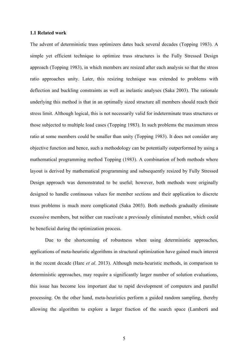
1

Simultaneous Topology, Shape and Size Optimization of

Truss Structures by Fully Stressed Design Based on

Evolution Strategy

This is the pre-print version of the published paper in “Engineering

Optimization” [1]. Some minor modifications were performed in the subsequent

stages.

[1] Ahrari, A., Atai, A. A., & Deb, K. (2014). Simultaneous topology, shape and size optimization of truss structures by fully stressed design based on evolution strategy. Engineering Optimization, (ahead-of-print), 1-22. http://dx.doi.org/10.1080/0305215X.2014.947972

Corrigendum:

The ground structure depicted for the 68-bar test problem (Figure 2f) has 73 bars. The

following 5 bars should not exist in the ground structure of this problem:

A3-5, A6-8, A9-11, A12-14, A15-17

where the subscripts denote the connecting nodes of the bars. Below is the corrected figure:

(1) (4) (7) (10) (13) (16)

(3) (6) (9) (12) (15) (18)

(8) (14)(5) (11)

5x120=600"

x

y

(17)(2)

2x40=80"

yFigure 2f (Corrected): Ground structure for the 68-bar test problem.

2

Simultaneous Topology, Shape and Size Optimization of Truss

Structures by Fully Stressed Design Based on Evolution Strategy

Ali Ahrari1*, Ali A. Atai2, Kalyanmoy Deb3

1Department of Mechanical Engineering, Michigan State University, East Lansing, MI, USA

2Department of Mechanical Engineering, University of Tehran, Tehran, Iran

3 Computational Optimization and Innovation (COIN) Laboratory, Department of Electrical and Computer Engineering, Michigan State University, East Lansing, MI, USA (http://www.egr.msu.edu/~kdeb

COIN Report Number 2015013

*Corresponding author, Email: aliahrari1983@gmail.com, Fax: +1-517-353-1750

Abstract The most effective scheme of truss optimization considers the combined

effect of topology, shape and size (TSS); however, most available studies on truss

optimization by meta-heuristics concentrated on one or two of the above aspects. The

presence of diverse design variables and constraints in TSS optimization may account

for such limited applicability of meta-heuristics to this field. In this article, a recently

proposed algorithm for simultaneous shape and size optimization, Fully Stressed

Design based on Evolution Strategy (FSD-ES), is enhanced to handle TSS optimization

problems. FSD-ES combines advantages of the well-known deterministic approach of

Fully Stressed Design with potential global search of the state-of-the-art ES. A

comparison of results demonstrates that the proposed optimizer reaches the same or

similar solutions faster and/or is able to find lighter designs than those previously

reported in the literature. Moreover, the proposed variant of FSD-ES requires no user-

based tuning effort which is desired in a practical application. The proposed

methodology is well tested on a number of problems and is now ready to be applied to

more complex TSS problems.

Keywords: fully stressed design; adaptive penalty; truss optimization benchmarks;

evolution strategies, resizing.

3

1 Introduction

Truss optimization can be considered from three distinct perspectives. Topology optimization

deals with selection of nodes and their connectivity. On another level, shape optimization

seeks to find the optimal coordinates of existing nodes. Finally, cross-sections of truss

members can be optimized, which is known as size optimization. In each case, the

optimization problem is subjected to some constraints on nodal displacements, member

stresses, critical buckling loads, natural frequencies, etc. The objective function is usually set

to minimize the structure weight which usually correlates with the overall cost.

While methods for shape and size optimization are quite similar in available truss optimizers,

a great variety of ideas for topology optimization have been developed in recent decades.

Shape annealing (Reddy and Cagan 1993) forms new topologies by employing some

predefined rules, called shape grammar, on an existing design. Shape and size variables are

also modified one-at-a-time using simulated annealing to direct the search process. A revised

version was applied to more intricate structures such as a transmission tower (Shea and Smith

2006) and a roof truss (Shea and Cagan 1999) by modifying the topology, shape and size.

However, flexibility of the topology optimization phase was quite limited.

In evolutionary structural optimization (ESO) (Xie and Steven 1993), the design

domain is discretized into 2D or 3D elements and inefficient element are gradually

eliminated. The improved version, called BESO (Huang and Xie 2007), allows for

reactivation of eliminated elements and smoothing of the topology. However, the whole

topology optimization strategy resembles a local search where the algorithm usually

converges to a close local optimum. Application of stochastic optimizers, which may provide

potent global search in cost of more evaluations, is not practical since this approach employs

a rather costly 2D or 3D finite element analysis. Additionally, the intricacy of the final

4

topology relies on the fineness of the mesh, and the BESO algorithm has four control

parameters to be tuned by the user.

The most common strategy to handle truss topology optimization is the ground

structure method (Topping 1983), where a subset of an excessively connected structure is

determined by the optimizer. Engineering intuition can be utilized to form a reasonable

ground structure for the problem at hand and evaluation is quite fast since FE analysis is

carried out using 1D elements, making it more desirable for population based optimizers. An

extension of this idea with a customized genetic algorithm as an optimizer has also been tried

(Deb and Gulati, 2001).

This study aims at reinforcing a recently introduced ES-based truss optimizer, called

Fully Stressed Design based on Evolution Strategy (FSD-ES), such that it can handle

simultaneous TSS problems as well. A variant of this algorithm, which handles only size and

shape optimization, outperforms existing shape and size optimizers (Ahrari and Atai 2013).

In particular, FSD-ES combines the reliable global search of meta-heuristics with engineering

knowledge on truss analysis to make the most of each evaluation. This enables it to handle

optimization of more complex structures with a large number of design variables. Moreover,

unlike most available TSS truss optimizers in literature which require an ad hoc tuning of

several control parameters for a new problem, the proposed FSD-ES is quasi parameter-free

from the user’s perspective.

The literature on TSS optimization employing the ground structure concept is

surveyed and a brief review of the available FSD-ES and other ES-based optimizers is

provided in section 2. The enhanced algorithm is elaborated in details in section 3. In section

4, a systematic experimentation on a selection of test problems is conducted and obtained

results from the proposed algorithm are compared to the best available results in the

literature.

5

1.1 Related work

The advent of deterministic truss optimizers dates back several decades (Topping 1983). A

simple yet efficient technique to optimize truss structures is the Fully Stressed Design

approach (Topping 1983), in which members are resized after each analysis so that the stress

ratio approaches unity. Later, this resizing technique was extended to problems with

deflection and buckling constraints as well as inelastic analyses (Saka 2003). The rationale

underlying this method is that in an optimally sized structure all members should reach their

stress limit. Although logical, this is not necessarily valid for indeterminate truss structures or

those subjected to multiple load cases (Topping 1983). In such problems the maximum stress

ratio at some members could be smaller than unity (Topping 1983). It does not consider any

objective function and hence, such a methodology can be potentially outperformed by using a

mathematical programming method Topping (1983). A combination of both methods where

layout is derived by mathematical programming and subsequently resized by Fully Stressed

Design approach was demonstrated to be useful; however, both methods were originally

designed to handle continuous values for member sections and their application to discrete

truss problems is much more complicated (Saka 2003). Both methods gradually eliminate

excessive members, but neither can reactivate a previously eliminated member, which could

be beneficial during the optimization process.

Due to the shortcoming of robustness when using deterministic approaches,

applications of meta-heuristic algorithms in structural optimization have gained much interest

in the recent decade (Hare et al. 2013). Although meta-heuristic methods, in comparison to

deterministic approaches, may require a significantly larger number of solution evaluations,

this issue has become less important due to rapid development of computers and parallel

processing. On the other hand, meta-heuristics perform a guided random sampling, thereby

allowing the algorithm to explore a larger fraction of the search space (Lamberti and

6

Pappalettere 2011). This enables handling of nonlinear, multimodal and discontinuous truss

problems, where deterministic approaches are prone to be trapped in undesirable local

minima. In contrast to mathematical programming approaches that can only eliminate a

member (Topping 1983), meta-heuristics may reactivate a removed member or node during

the optimization process. Additionally, structural optimization is seldom a continuous

variable problem, which highly limits the applicability of gradient-based methods.

Most previous studies on truss optimization by meta-heuristics, even those published

recently, deal with truss optimization on one or two levels. For example, size optimization by

Harmony Search algorithm (Lee et al. 2005, Degertekin 2011), Artificial Bee Colony

(Sonmez 2011), Big-Bang-Big Crunch algorithm (Kaveh and Talatahari 2009b), Reduced

Space and Sequential Quadratic Programming (Chen and Huang 2012), Charged System

Search (Kaveh and Talatahari 2010), Chaotic Imperialist Competitive Algorithm (Talatahari

et al. 2012), evolution strategies (Papadrakakis et al. 1998), Particle Swarm Optimization (Li

et al. 2007, Lu et al. 2012), Genetic Algorithm (Toğan and Daloğlu 2008), Ant Colony

Optimization (Kaveh et al. 2008), and also some hybridized algorithms (Ayvaz et al. 2009,

Kaveh and Talatahari 2009a, Rahami et al. 2011) are worth mentioning. Hasançebi et al.

(2009) compared performance of seven different stochastic optimization techniques for size

optimization of truss structures and concluded that evolution strategies and Simulated

Annealing are the most reliable approaches.

More sophisticated schemes consider the joint effect of shape and size (Hasançebi

2008, Farajpour 2011, Kaveh and Talatahari 2011, Lee et al. 2011, Miguel and Miguel 2012,

Kaveh and Khayatazad 2013), or topology and size (Ruiyi et al. 2009, Su et al. 2011).

Nevertheless, studies on simultaneous topology, shape and size (TSS) optimization are

comparatively scarce, although this is the most rigorous, complete, and effective scheme

(Luh and Lin 2008). The diversity in the types of design variables may account for this trend.

7

Boolean, continuous and discrete variables should be reasonably employed for topology,

shape and size optimization, respectively (Rajan 1995). Additionally, the number of design

variables grows excessively for more intricate structures, which quite often demands a large

population size (Deb and Gulati 2001, Hultman 2010). Accordingly, some techniques aimed

at alleviating problem complexity of TSS optimization of truss structures have emerged

during the past decade, a number of which are discussed.

Genetic Algorithms (GAs) have been widely utilized in TSS optimization of truss

structures (Rajan 1995, Deb and Gulati 2001, Rahami et al. 2008, Hultman 2010). When

using Binary-coded GAs (BGAs), continuous variables are discretized (Rahami et al. 2008),

for which the discretization step, which determines precision of the optimized results, should

be tuned. Deb and Gulati (2001) proposed a real-valued GA in which the search range of

member areas is assumed symmetric, for example, [-A, A], and members with areas less than

a predefined threshold, +ε, are considered passive, i.e. eliminated from in the structure. This

strategy was also employed in some recent studies (Luh and Lin 2008, Wu and Tseng 2010),

resulting in continuous treatment of all variables.

Another strategy to moderate problem complexity of TSS optimization is to use a

two-stage approach. First, the structure topology is optimized while the cross-sectional area

of members and shape of the truss remain fixed. After an optimized topology is found, size as

well as shape of the obtained topology is optimized. Such a strategy greatly alleviates the

problem complexity as it reduces the number of object variables at each stage. Luh and Lin

(2008, 2011) exploited this strategy for TSS optimizing using Ant Colony or Particle Swarm

Optimization methods. Although for the investigated problems this two-stage strategy

appeared beneficial, it cannot always provide the global optimum since TSS optimization is

not a separable problem (Deb and Gulati 2001, Rahami et al. 2008). The obtained results

were outperformed by another method based on Differential Evolution (Wu and Tseng 2010),

8

which considers the joint effects of topology, shape and size. Nonetheless, in the latter

research, the drawbacks of continuous values for member areas and specifying the critical

area, ε, remained unsolved.

A remarkably efficient strategy is to activate or deactivate a non-basic node or

member, a node or member that can be eliminated, with similar probabilities (Hasançebi and

Erbatur 2002a, Hasançebi 2007). This strategy leads to an inherent bias towards topologies

with small number of nodes and members, since the number of acceptable topologies in

which a non-basic node is active is much more than those where this node is passive.

Noilublao and Bureerat (2011) applied multi-objective EAs on TSS optimization of a

slender truss tower, where a second objective is introduced using either the natural

frequencies, frequency response function (FRF), or force transmissibility (FT). Sequential

cellular particle swarm optimization (SCPSO), suggested by Gholizadeh (2013), provided

good solutions for some TSS test problems. However, the algorithm needed tuning of five

control parameters and selection of a grid for each problem. The large amount of tuning

required substantially diminishes the practicality and robustness of the algorithm. The firefly

algorithm (FA) (Miguel et al. 2013), in contrast, has a few control parameters and thus more

practical, but the best solutions found by this method were slightly heavier.

2 Evolution Strategies and ES-based Truss Optimizers

One of the main streams of evolutionary algorithms, the evolution strategies (ES), follows the

principles of natural selection, including recombination, mutation and selection. In the

canonical form, a number of λ offspring are produced by recombination and mutation of µ

(usually less than λ) parents. Selection is performed over the recently generated offspring

(“Comma” scheme), or the combination of parents and offspring (“Plus” scheme). These two

schemes are denoted by (µ/ρ,λ)-ES and (µ/ρ+λ)-ES respectively. The extra parameter, ρ,

specifies the number of parents that recombine to generate each offspring. More details on ES

9

and their variants can be found in a comprehensive review by Beyer and Schwefel (2002).

Among ES variants, Covariance Matrix Adaptation Evolution Strategy (CMA-ES), is

considered as the state-of-the-art ES for unconstrained continuous optimization (Beyer and

Sendhoff 2008, Kramer 2010). This optimizer ranked the best among the optimization

algorithms that participated in the CEC-05 (García et al. 2009) and BBOB-2009 (Hansen et

al. 2010b) workshops. CMA-ES employs normal distribution for sampling, mutates all

variables simultaneously, performs non-elite (“Comma”) selection, recombines design

variables using Global Weighted Recombination (GWR), and adapts the covariance matrix of

sampling distribution. However, TSS optimization problems are neither unconstrained nor

continuous and some of the peculiar features of ES, and CMA-ES in particular, are inevitably

modified while tailoring them for truss optimization. For example, in many previous studies,

a discrete distribution replaced the normal distribution (Hasançebi 2008, 2009, Thierauf and

Cai 1998, Lagaros et al. 2002), the discrete recombination replaced the intermediate

recombination for size variables (Papadrakakis et al. 1998, Thierauf and Cai 1998, Lagaros et

al. 2002, Ebenau et al. 2005, Hasançebi 2008, Hasançebi et al. 2009), only a fraction of

variables were mutated (Lagaros et al. 2002, Papadrakakis et al. 1998, Ebenau et al. 2005,

Hasançebi 2007, 2008, Hasançebi et al. 2009), or the elite individuals were preserved

(Hasançebi 2008, Ebenau et al. 2005).

Unlike previous efforts for truss optimization by ES, FSD-ES tries to abide by the

principles of the state-of-the-art ES (Ahrari and Atai 2013). The next section elaborates the

steps of the reinforced FSD-ES, which can handle topology optimization as well.

3 FSD-ES for simultaneous TSS optimization

In this section the problem representation, algorithm steps, and rationale underlying each

strategy are explained in detail so that the role of each part is clarified and that the results are

reproducible. Some concepts and relations are quite similar to those utilized in the earlier

10

version (Ahrari and Atai 2013), however, the new variant of this algorithm can encompass

TSS optimization problems as well.

3.1 Problem Representation

In FSD-ES, each candidate design is configured by three vectors:

- M1×e is a vector of Boolean variables that determines connection of members in a candidate

design.

- X1×3n is a vector of continuous variables that determines nodal coordinates.

- A1×e is a vector of continuous/discrete variables that determines member areas.

Parameters e and n denote the number of members and nodes in the ground structure,

respectively. Such representation resembles the work of Rajan (1995), where Boolean,

continuous, and discrete variables were allocated for topology, shape, and size respectively.

Matrices M=[mji]2λ×e, X=[mji]2λ×3n, A=[aji]2λ×e store the values of topology, shape and size of

all individuals in the current iteration, where 2λ is the population size.

3.2 Initial Values

For the first iteration, recombinant design can be randomly selected within the bounds. As

this design is not evaluated, it does not necessarily belong to the given discrete set. The

recombinant point, denoted by the subscript R, consists of vectors of design variables (MR,

XR, AR) and their corresponding vectors of strategy variables (σMR, σXR, σAR). An independent

mutation step is allotted for each design variable. The values of the strategy variables are set

to a fraction of the corresponding search range: 1/2, 1/3, and 1/4 for Boolean, discrete, and

continuous variables, respectively.

3.3 Mutating topology variables

First, the strategy parameters of topology variables are mutated:

σMj=exp(τ0Nj)(σMR⊗[exp(τN(0,1)) … exp(τN(0,1))]) (1)

where the sign ⊗ refers to element-wise multiplication, the index j refers to the j-th

11

individual, σMj is the vector of step sizes for topology variables of this individual, Nj is a

random number sampled from the standard normal distribution, τ0 and τ are learning rates

which are set to 0.5(NVAR)-0.5 and 0.5(NVAR)-0.25 respectively. NVAR is the total number of

(independent) design variables, equal to the sum of the number of topology (Ntop), shape

(Nshape) and size (Nsize) variables. Nshape and Nsize are set to the number of independent

coordinates and member section variables respectively. The value of Ntop, however, is the

binary logarithm of the number of topologically distinct acceptable designs1.

Once the value of σMj is determined, it is used to mutate topology variables. The

truncated normal distributions are used to sample Mj. The centre of mutation is MR, the

standard deviation is σMj, and [0, 1] is the truncated range. Since Mj consists of Boolean

variables, a rounding strategy is subsequently performed. Unlike conventional rounding

strategies which replace the continuous variable by the closest (scaled) discrete value (Chen

and Chen 2006), a stochastic rounding technique is used in which each component of Mj

becomes 1 with the probability of its value and 0 otherwise. This kind of rounding does not

change the expected value of that component.

After rounding, the generated topology, Mj, is accepted if it is stable and includes

basic nodes of the structure, otherwise discarded and this step starts again from the

beginning. To check stability, the condition number of the stiffness matrix of the generated

topology is calculated while the shape and size of the design are equal to their corresponding

values in the recombinant design. If the condition number is larger than a predefined value,

e.g. 1010, the design is considered unstable.

1 This can be easily estimated by uniform sampling of a reasonable number of topologies (for example

1,000) subset of the ground structure and calculating the ratio of the acceptable topologies to all

sampled topologies. As the overall number of topologies is known, the number of acceptable

topologies can easily be estimated.

12

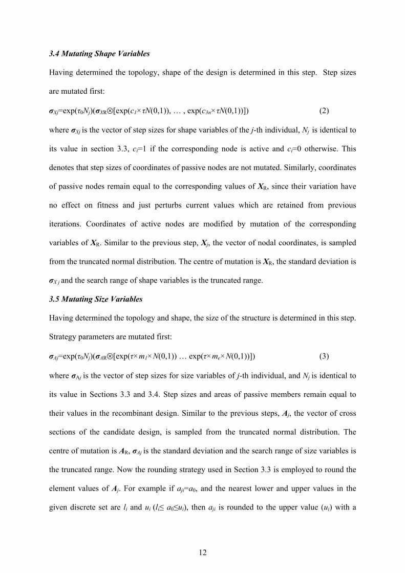
3.4 Mutating Shape Variables

Having determined the topology, shape of the design is determined in this step. Step sizes

are mutated first:

σXj=exp(τ0Nj)(σXR⊗[exp(c1×τN(0,1)), … , exp(c3n×τN(0,1))]) (2)

where σXj is the vector of step sizes for shape variables of the j-th individual, Nj is identical to

its value in section 3.3, ci=1 if the corresponding node is active and ci=0 otherwise. This

denotes that step sizes of coordinates of passive nodes are not mutated. Similarly, coordinates

of passive nodes remain equal to the corresponding values of XR, since their variation have

no effect on fitness and just perturbs current values which are retained from previous

iterations. Coordinates of active nodes are modified by mutation of the corresponding

variables of XR. Similar to the previous step, Xj, the vector of nodal coordinates, is sampled

from the truncated normal distribution. The centre of mutation is XR, the standard deviation is

σX j and the search range of shape variables is the truncated range.

3.5 Mutating Size Variables

Having determined the topology and shape, the size of the structure is determined in this step.

Strategy parameters are mutated first:

σAj=exp(τ0Nj)(σAR⊗[exp(τ×m1×N(0,1)) … exp(τ×me×N(0,1))]) (3)

where σAj is the vector of step sizes for size variables of j-th individual, and Nj is identical to

its value in Sections 3.3 and 3.4. Step sizes and areas of passive members remain equal to

their values in the recombinant design. Similar to the previous steps, Aj, the vector of cross

sections of the candidate design, is sampled from the truncated normal distribution. The

centre of mutation is AR, σAj is the standard deviation and the search range of size variables is

the truncated range. Now the rounding strategy used in Section 3.3 is employed to round the

element values of Aj. For example if aji=a0, and the nearest lower and upper values in the

given discrete set are li and ui (li≤ a0≤ui), then aji is rounded to the upper value (ui) with a

13

probability of (aji-li)/(ui-li) and to the lower value (li) otherwise.

3.6 Evaluation

In this step, the generated design is evaluated and member stresses and nodal deflections are

computed:

𝑮! = 𝑔!" ,𝑔!" =𝜎!"/𝜎!"!    if  𝑚!" = 10                            if  𝑚!" = 0

  , 𝑖 = 1,2,… , 𝑒

𝑯! = ℎ!" , ℎ!" =𝑓!"/𝑓!"!    if  𝑚!" = 1  and  𝜎!" < 00                            otherwise                                          

,      𝑖 = 1,2,… , 𝑒                                                              (4)

𝑼! = 𝑢!" ,𝑢!" =𝛿!"/𝛿!"!    if  coordinate  𝑘  of  design  𝑗  is  active0                              otherwise                                                                                              

,      𝑘 = 1,2,… ,3𝑛

Vectors Gj, Hj and Uj store the ratios of calculated stress (σij), square root of the buckling load

(fij ), and nodal deflection (δij) to their allowable limits respectively. For a feasible design, all

elements are equal to or less than one, otherwise some nodes or members have violated some

constraints. For constraint violations, a penalty term is used knowing that the optimal design

falls on or very close to the boundary of the feasible region. In comparison with death penalty

that has been used in some previous studies (Deb and Gulati 2001, Luh and Lin 2008; 2011)

an adaptive penalty term enables the search process to approximate this area from both sides

(Ebenau et al. 2005). Following this goal and utilization of engineering knowledge on truss

analysis, a penalty term that is tailored for truss optimization is defined. For any arbitrary

positive number (α>0), the following assumptions are utilized:

- Nodal deflections are divided by α if all areas are multiplied by α.

- Member stress is divided by α if the area of that element is multiplied by α

- Member critical buckling load is divided by α2, if the area of that element is

multiplied by α.

The first assumption is valid for both determinate and indeterminate trusses while the second

14

and third assumptions are valid only for determinate trusses. Nevertheless, they can still be

partially utilized knowing that the optimal topology would have a low degree of

indeterminacy. Using these assumptions, the required amount of increase in member area

such that all constraints are satisfied can be computed. For example, if gj2=1.4, aj2 should be

multiplied by 1.4 so that the 2nd member of the j-th design satisfies the stress constraint. If so,

the overall volume of the structure is increased by 0.4aj2lj2, where lj2 is the length of the j-th

member. The penalized objective function is defined as follows:

𝑓! =𝑊! + 𝜌 𝑐!"𝑎!"𝑙!" 𝑞!"! − 1!

!!!

, 𝑞!" = max 1,𝑔!" , ℎ!" ,max 𝑼!                                      (5)  

This equation implies that if areas of all members are multiplied by the corresponding qji,

the resultant truss supposedly satisfies all constraints. This leads to an increase of

𝑙!"𝑎!"(𝑞!" − 1)!!!! in the volume of design j, which depends not only on the constraint

violation amount, but also on the current length and cross section of that member. This means

similar constraint violation for a larger member results in a larger penalty term. Parameter

cPi≥0.5 intensifies the penalty and controls the resizing rate, which is explained in Step 3.7.

3.7 Resizing

Following the deterministic method of Fully Stressed Design, a resizing step is performed to

generate new individuals. In this step, vectors Gj, Hj and Uj calculated in the previous step

are utilized to generate a supposedly near-boundary design from the j-th design by changing

only the size variables. Member forces are assumed to be constant, and each member section

is resized such that the stress or buckling constraints become activated, which means the

member should be loaded up to its maximum capacity. However, reduction of member areas

takes place more conservatively since, as discussed earlier, not all members may reach their

stress limit in the optimum design. The shrinking rate of the member area is controlled by cPi.

For cPi=0.5 (minimum value), each member area is shrunk so that stress or buckling

15

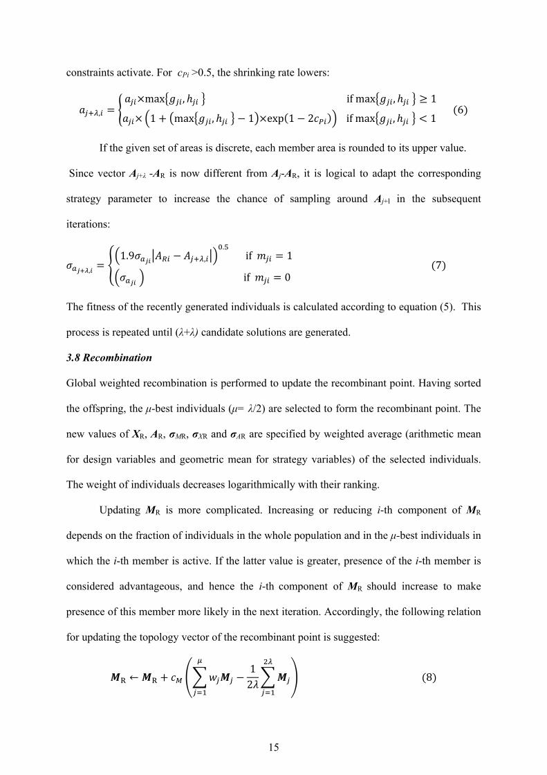
constraints activate. For cPi >0.5, the shrinking rate lowers:

𝑎!!!,! =𝑎!"×max 𝑔!" , ℎ!"                                                                                                                      if  max 𝑔!" , ℎ!"   ≥ 1

𝑎!"× 1+ max 𝑔!" , ℎ!"   − 1 ×exp 1− 2𝑐!"      if  max 𝑔!" , ℎ!"   < 1            (6)

If the given set of areas is discrete, each member area is rounded to its upper value.

Since vector Aj+λ -AR is now different from Aj-AR, it is logical to adapt the corresponding

strategy parameter to increase the chance of sampling around Aj+l in the subsequent

iterations:

𝜎!!!!,! =1.9𝜎!!" 𝐴!" − 𝐴!!!,!

!.!            if    𝑚!" = 1

𝜎!!"                                                                                  if    𝑚!" = 0                                                                                                                  (7)

The fitness of the recently generated individuals is calculated according to equation (5). This

process is repeated until (λ+λ) candidate solutions are generated.

3.8 Recombination

Global weighted recombination is performed to update the recombinant point. Having sorted

the offspring, the µ-best individuals (µ= λ/2) are selected to form the recombinant point. The

new values of XR, AR, σMR, σXR and σAR are specified by weighted average (arithmetic mean

for design variables and geometric mean for strategy variables) of the selected individuals.

The weight of individuals decreases logarithmically with their ranking.

Updating MR is more complicated. Increasing or reducing i-th component of MR

depends on the fraction of individuals in the whole population and in the µ-best individuals in

which the i-th member is active. If the latter value is greater, presence of the i-th member is

considered advantageous, and hence the i-th component of MR should increase to make

presence of this member more likely in the next iteration. Accordingly, the following relation

for updating the topology vector of the recombinant point is suggested:

𝑴! ← 𝑴! + 𝑐! 𝑤!𝑴!

!

!!!

−12𝜆 𝑴!

!!

!!!

                                                                                                   (8)

16

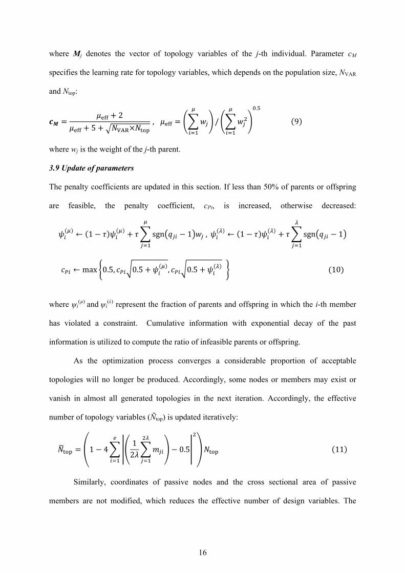
where Mj denotes the vector of topology variables of the j-th individual. Parameter cM

specifies the learning rate for topology variables, which depends on the population size, NVAR

and Ntop:

𝒄𝑴 =𝜇!"" + 2

𝜇!"" + 5+ 𝑁!"#×𝑁!"#  ,      𝜇!"" = 𝑤!

!

!!!

/ 𝑤!!!

!!!

!.!

                                9

where wj is the weight of the j-th parent.

3.9 Update of parameters

The penalty coefficients are updated in this section. If less than 50% of parents or offspring

are feasible, the penalty coefficient, cPi, is increased, otherwise decreased:

𝜓!! ← 1− 𝜏 𝜓!

! + 𝜏 sgn 𝑞!" − 1 𝑤!  ,!

!!!

 𝜓!! ← 1− 𝜏 𝜓!

! + 𝜏 sgn 𝑞!" − 1!

!!!

𝑐!" ← max 0.5, 𝑐!" 0.5+ 𝜓!! , 𝑐!" 0.5+ 𝜓!

!                                                                                                                (10)

where ψi

(µ) and ψi(λ) represent the fraction of parents and offspring in which the i-th member

has violated a constraint. Cumulative information with exponential decay of the past

information is utilized to compute the ratio of infeasible parents or offspring.

As the optimization process converges a considerable proportion of acceptable

topologies will no longer be produced. Accordingly, some nodes or members may exist or

vanish in almost all generated topologies in the next iteration. Accordingly, the effective

number of topology variables (Ñtop) is updated iteratively:

𝑁!"# = 1− 412𝜆 𝑚!"

!!

!!!

− 0.5

!!

!!!

𝑁!"#                                                                                                                               11

Similarly, coordinates of passive nodes and the cross sectional area of passive

members are not modified, which reduces the effective number of design variables. The

17

effective number of shape variables (Ñshape) and the effective number of size variables (Ñsize)

are set to the average number of independent active coordinates and size variables

respectively. Since the effective number of design variables has changed, the learning rates

for the next iteration are updated:

𝜏! ←1

2 𝑁!"#, 𝜏 ←

1

2 𝑁!"#! , 𝑐! ←

𝜇!"" + 2

𝜇!"" + 5+ 𝑁!"#×𝑁!"#                          (12)

where ÑVAR=Ñtop+Ñshape+Ñsize is the updated value for the effective number of design

variables.

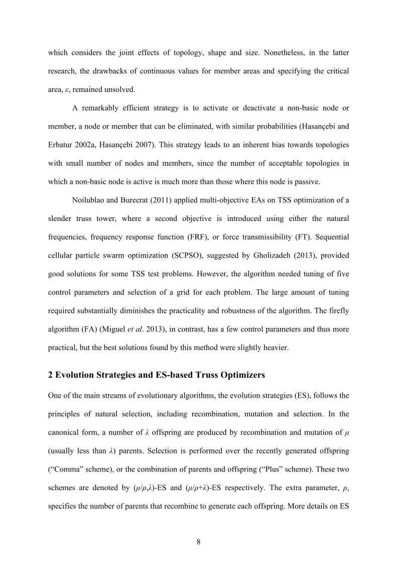
Figure 1. Flowchart for FSD-ES.

Initialize the recombinant design and the

corresponding strategy parameters.

Generate a candidate topology by

mutation of the recombinant topology

Determine the candidate shape by

mutation of the recombinant shape

Is the topology

acceptable?

Determine the candidate size by mutation

of the recombinant size

Calculate the objective function and

constraints

Has the algorithm

converged?

Form a new individual by resizing the

recently generated candidate design

Select the best µ individuals and update

design and strategy parameters

End

No

Yes

No

Yes

Have 2λ designs

been generated?

Yes

No

Start

18

3.10 Convergence Check

Several effective convergence checks based on statistical criteria has been proposed (Hansen

2009), yet according to performance measures employed in this study, the algorithm

terminates when it reached the maximum number of iterations, otherwise it is resumed from

Section 3.3. FSD-ES does not use any information on the iteration number or maximum

number of iterations to adjust strategy parameters. The flowchart for FSD-ES is provided in

Figure 1.

4 Empirical evaluation

In this section, a number of qualitatively distinct problems are selected, on which FSD-ES is

evaluated and compared with the most competent methods in the literature.

4.1 Test problems

Test problems considering only one aspect of truss optimization are excluded as the

concentration of this article is on TSS optimization problems. Some prevalent, albeit too

simple, test problems are excluded and a brief explanation that highlights distinctive features

of each selected test problem is presented.

The first problem is a 45-bar 2D truss employed by Deb and Gulati (2001). The structure

weight is minimized while symmetry is ignored. The ground structure, depicted in Figure 2a,

has an all pair-wise interconnection (all-to-all scheme). A vertical load of 10 kips is exerted

on nodes 7, 8 and 9. Member areas may take any values within [0.09,1] in2. The maximum

deflection and axial stress are limited to 2 in. and 25 ksi. The density and modulus of

elasticity are 0.1 lb/in3 and 10000 ksi respectively.

The second test is a TSS optimization problem adapted from (Rahami et al. 2008).

The 15-bar ground structure is depicted in Figure 2b. This is quite a simple TSS problem

since node 4 is intuitively redundant and other nodes may not be eliminated. Data required

for simulation of this problem is presented in Table 1.

19

Table 1. Simulation data for the 15-bar truss problem. Design

Variables Shape (8) x2=x6; x3=x7; y2; y3; y4; y6; y7; y8 Size (15) Ai , i=1,2,…,15

Constraints Stress (σc)i ≤172.4 MPa (25 ksi); (σt)i ≤172.4 MPa (25 ksi), i=1,2,…,15 Displacement None Buckling None

Search Range

Shape Variables

254 cm (100 in) ≤ x2 ≤ 355.6 cm (140 in.); 558.8 cm (220 in.) ≤ x3 ≤ 660.4 cm (260 in.); 254 cm (100 in.) ≤ y2 ≤ 355.6 cm (140 in.); 254 cm (100 in.) ≤ y3 ≤ 355.6 cm (140 in.); 127 cm (50 in.) ≤ y4 ≤ 228.6 cm (90 in.); −50.8 cm (−20 in.) ≤ y6 ≤ 50.8 cm (20 in.); −50.8 cm (−20 in.) ≤ y7 ≤ 50.8 cm (20 in.); 50.8 cm (20 in.) ≤ y8 ≤ 152.4 cm (60 in.);

Size Variables

Ai∈S , i = 1, . . . , 15 S={0.111, 0.141, 0.174, 0.22, 0.27, 0.287, 0.347, 0.44, 0.539, 0.954, 1.081, 1.174, 1.333, 1.488, 1.764, 2.142, 2.697, 2.8, 3.131, 3.565, 3.813, 4.805,5.952, 6.572, 7.192, 8.525, 9.3, 10.85, 13.33, 14.29, 17.17, 19.18} (in.2) S={0.716, 0.910, 1.123, …, 123.742} (cm2)

Loading Nodes Fx Fy 8 - −44.537 KN (−10.0 kips)

Mechanical Properties Modulus of elasticity: E=68.95 GPa (1.0×104 ksi) Density of the material: ρ=0.0272 N/cm3 (0.1 lb/in.3)

The third problem is a simultaneous TSS optimization of a 25-bar spatial truss

adapted from (Rahami et al. 2008). Front and left views of the ground structure are depicted

in Figure 2c. The structure, but not the loading, is symmetric with respect to the xz and yz

planes, which reduces the number of independent sections and coordinates to 8 and 5

respectively. Table 2 presents data required for simulation of this problem.

The fourth test is a two-tier 39-bar truss proposed by Deb and Gulati (2001) and

subsequently used in many recent studies (Luh and Lin 2008, Wu and Tseng 2010, Luh and

Lin 2011) as a more comprehensive TSS optimization problem. The symmetric ground

structure is depicted in Figure 2d in which overlapping members are illustrated with curved

line segments. The coordinates of nodes 1, 2, 3, 4 and 5 are fixed and node 11 is allowed to

move vertically. The coordinate variables may vary up to ±120 inch with respect to their

value in the ground structure. Structural symmetry is exploited to shrink the number of design

variables. The range of available section areas is assumed to be continuous, where 0.05 and

2.25 in2 are the lower and upper limits of this range. A vertical load of P=20 kips is exerted

on nodes 2, 3 and 4. In comparison with the previous test, the number of design variables has

increased. The problem has a low-fitness local optimum (W~214 lb) with minimal number of

active nodes (7), which can trap algorithms that inherently favour simpler topologies.

20

100

P P P(10) (9) (8) (7) (6)

(5)(4)(3)(2)

(1)

4x100=400

10

(5)P

(6) (7)(8)

(4)(3)(2)(1)

11

1

4

7 8

5

13

12

2

9

6

15

14

3

x

y

120

3x120=360

(a) (b)

4x120=480

2x12

0=24

0

(10)(11)(12)

(9) (8) (7) (6)

(5)(4)(3)(2)

PPP

(1)

ground structure

(c) (d)

yx

3x120=360

4x60=240

5x60=300

(1)(3)(5)(7)

(8) (6) (4) (2)

(9)(11)(13)

(14) (12) (10)

(15)

(17)

(19)

(21)

(22)

(20)

(18)

(16)

159

12

11

8

7

4

3

2610

15

16

14

13172125

31

33

35

29

39

30

36 38

2834

32

2624 20

23 19

4043 44 46 4745

1822

27

37

41 42

(e)

(1) (4) (7) (10) (13) (16)

(3) (6) (9) (12) (15) (18)

(8) (14)(5) (11)

5x120=600

x

y

(17)(2)

2x40=80 (8) (14)(5) (11)

(f)

Figure 2. Ground structure for test problems 1 to 4: a) 45-bar truss, b) 15-bar truss, c) 25-bar spatial truss (front

and left view), d) 39-bar truss, e) 47-bar truss and f) 68-bar truss test problems.

21

Table 2. Simulation data for the 25-bar spatial truss problem.

Design Variables Shape (5) x4=x5=−x3=−x6 ; x8=x9=−x7=−x10 ; y3=y4=−y5=−y6 ; y7=y8=−y9=−y10 ; z3=z4=z5=z6 Size (8) ai , i=1,2,…,8 (Other member areas are dependent to these 8 variables)

Constraints Stress (σc)i ≤275.8 MPa (40 ksi); (σt)i ≤275.8 MPa (40 ksi), i=1,2,…,25 Displacement ui≤0.89 cm (0.35 in) Buckling None

Search Range Shape Variables

50.8 cm (20 in.) ≤ x4 ≤ 152.4 cm (60 in.) ; 101.6 cm (40 in.) ≤ x8 ≤ 203.2 cm (80 in.) ; 101.6 cm (40 in.) ≤ y4 ≤ 203.2 cm (80 in.) ; 254 cm (100 in.) ≤ y8 ≤ 355.6 cm (140 in.); 228.6 cm (90 in.) ≤ z4 ≤ 330.2 cm (130 in.)

Size Variables Ai∈S , i = 1, . . . , 25 S={0.1, 0.2, 0.3, … , 2.6} U {2.8, 3.0, 3.2, 3.4} (in.2)

Loading

Nodes Fx KN (kips) Fy KN (kips) Fz KN (kips) 1 2 3 6

4.454 (1.0) 0.0 2.227 (0.5) 2.672 (0.6)

-44.537 (-10.0) -44.537 (-10.0) 0.0 0.0

-44.537 (-10.0) -44.537 (-10.0) 0.0 0.0

Mechanical Properties Modulus of elasticity: E=68.95 GPa (1.0×104 ksi) Density of the material: ρ=0.0272 N/cm3 (0.1 lb/in.3)

The fifth problem is size and shape optimization of a 47-bar power line truss adapted

from the work of Hasançebi and Erbatur (2002b). Problem specifications are presented in

Table 3 and the ground structure is depicted in Figure 2e. The structure is supposed to be able

to carry three load cases. External load is not symmetric, but the structure design including

nodal coordinates and member cross sections are symmetric. Coordinates of nodes 15, 16, 17

and 18 are fixed. The ranges of coordinate variables were not quoted in the referenced paper

and hence, a logical range was selected for this study.

Table 3. Data for simulation of the 47-bar truss problem.

Design Variables

Shape (17) -x1=x2 ; -x3=x4 , y3=y4 ; -x5=x6 , y5=y6 ; -x7=x8 ; y7=y8 ; -x9=x10 ; y9=y10 ; -x11=x12 ; y11=y12 ; -x13=x14 ; y13=y14 ; -x19=x20 ; y19=y20 ; -x21=x22 ; y21=y22

Size (27) Ai=Ai-1 , i=2,4,6,…,20 ; A41 , A42 , A43 , A44 , A45 , A46 , A47

Constraints Stress (σc)i ≤103.4 MPa (15 ksi); (σt)i ≤137.9 MPa (20 ksi), i=1,2,…,47 Displacement None Buckling |(σc)i|≤αEai/li

2 , i=1,2,…,47 , α=3.96

Search Range

Shape Variables

0 ≤ x2, x4, x6, x8 ≤ 381.0 cm (150 in.) ; 0 ≤ x10, x12, x14 ≤ 190.5 cm (75 in.) 0 ≤ x22 ≤ 190.5 cm (75 in.) ; 0 ≤ x20 ≤ 381.0 cm (150 in.) ; 0 ≤ y4 ≤ 609.6 cm (240 in.) ; 304.8 cm (120 in.) ≤ y6 ≤ 914.4 cm (360 in.) ; 609.6 cm (240 in.) ≤ y8 ≤ 1066.8 cm (420 in.) ; 914.4 cm (360 in.) ≤ y10 ≤ 1219.2 cm (480 in.) 1066.8 cm (420 in.) ≤ y12 ≤ 1371.6 cm (540 in.) ; 1219.2 cm (480 in.) ≤ y14 ≤ 1524.0 cm (600 in.) 1371.6 cm (540 in.) ≤ y20 , y22 ≤ 1676.4 cm (660 in.)

Size Variables Ai∈S , i = 1, . . . , 47 S={0.1,0.2,0.3,…,4.9,5} (in.2) S={0.645,12.903,…,32.258} (cm2)

Loading

Nodes Fx Fy Case I 17,18 26.689 KN (6 kips) -62.275 KN (-14.0 kips) Case II 17 26.689 KN (6 kips) -62.275 KN (-14.0 kips) Case III 18 26.689 KN (6 kips) -62.275 KN (-14.0 kips)

Mechanical Properties Modulus of elasticity: E=206.84 GPa (3.0×104 ksi) Density of the material: ρ=0.081434 N/cm3 (0.3 lb/in.3);

The sixth test is TSS optimization of a 68-bar truss subjected to two load cases at the

end. Data required for simulation of this problem is presented in Table 4. Horizontal and

22

vertical coordinates of the nodes may vary within 120 and 40 in. of the initial configuration

respectively (Figure 2f). The ground structure allows elimination of most members and nodes

except nodes 1, 3, and 17. This test problem is introduced in this study and has a significantly

larger number of design variables compared to the previous test problems.

Table 4. Data for simulation of the 68-bar truss problem.

Design Variables Shape (31) y17, xi, yi, i=2,4,5,6,…, 14,15,16,18 Size (68) ai , i=1,2,…,68

Constraints Stress (σc)i ≤137.9 MPa (20 ksi); (σt)i ≤137.9 MPa (20 ksi), i=1, 2, …, 68 Displacement uj≤2.5 in., j=1, 2, 3, …, 68 Buckling |(σc)i|≤αEai/li

2 , i=1,2,…,68, α=3.96

Search Range

Shape Variables Horizontal coordinates may vary within ±120 in of their initial value. Vertical coordinates may vary within ±40 in of their initial value.

Size Variables

Ai∈S , i = 1, . . . , 68 S={0.111, 0.141, 0.174, 0.22, 0.27, 0.287, 0.347, 0.44, 0.539, 0.954, 1.081, 1.174, 1.333, 1.488, 1.764, 2.142, 2.697, 2.8, 3.131, 3.565, 3.813, 4.805, 5.952, 6.572, 7.192, 8.525, 9.3, 10.85} (in.2) S={0.716, 0.910, …, 70.0} (cm2)

Loading Nodes Fx Fy KN (kips)

Case I Case II

17 17

222.41 KN (-50 Kip) 222.41 KN (-50 Kip)

0 -66.72 KN (-15 Kip)

Mechanical Properties Modulus of elasticity: E=206.84 GPa (3.0×104 ksi) Density of the material: ρ=0.081434 N/cm3 (0.3 lb/in.3);

4.2 Evaluation method

The performance measure employed in this article is based on the Expected Running Time

(ERT) to reach a predefined tolerance of the global minimum, as discussed and advocated by

Hansen et al. (2010):

ERT(ftarget)=((SR)(FES)+(1-SR)(FEUS))/SR (13)

where SR is the success rate, which is the fraction of independent runs in which the algorithm

could reach ftarget. FES is the average number of function evaluations of successful runs to

reach ftarget, and FEUS represents the average number of function evaluations of unsuccessful

runs. ERT facilitates comparison of optimization methods since it considers the overall

effects of reliability and convergence speed. To utilize equation (13), the algorithm should

stop when it reaches a certain tolerance of the objective function or when the convergence

criterion is met. However, in truss optimization, as with most practical problems, the global

23

optimum is not known and besides, the performance measure should discriminate between

converging to a high/low fitness minimum. Accordingly, the optimization algorithm is run

for a long time and the required number of evaluations to reach different structural weights is

recorded. FEUS~FES is a logical assumption (Auger and Hansen 2005), which simplifies

equation (13) to the following:

ERT(ftarget)= FES/(SR). (14)

In this study, the above equation is used to calculate ERT from FES and SR at any arbitrary

target function value. The ERT plots in this case can discriminate and compare both the short

and long term performance of algorithms. Such discrimination is of great practical interest as

the budget of function evaluations determines whether short or long-term success is desired.

4.3 Parameter tuning

All control parameters of FSD-ES are set to their recommended values as described in

section 3 except the population size, which should ideally be proportional to the problem

complexity. The population size (λ) is set using the following relation, which considers the

number of design variables and constraints:

K1 = Ntop+Nshape+Ǹsize+(Ntop×Nshape)0.5+(Nshape×Ǹsize)0.5+( Ǹsize ×Ntop)0.5+( Ntop×Nshape×Ǹsize).333

K2 = (zdef×e×Ǹsize/Nsize+zstress×n×d)×Nload×d

λ=[(0.2×K1×K2)0.5+5.5] (15)

where Ǹsize = Nsize - 0.5×Ntop is the adjusted number of size variables. K1 and K2 are based on

the complexity caused by the number of design variables and constraints respectively. d is the

space dimension, which is 2 for planar and 3 for spatial structures, and Nload represents the

number of load cases. e and n are the number of members and nodes in the ground structure

and zdef is 1 if nodal deflections are constrained and 0 otherwise. Similarly, zstress is 1 if

members are subject to stress or buckling constraints and 0 otherwise. Following the

24

procedure explained in section 3.3, the estimated value for Ntop is 43.4, 8.25, 3.55, 18.94, 0,

and 65.5, which leads to the population size of 35, 22, 39, 44, 66, and 136 for problems 1 to 6

respectively. The optimization process is terminated after 20λ+100 iterations; however, as

emphasized earlier, ERT, SR and FES for specific target weights are to be compared.

Accordingly, FSD-ES requires no ad hoc tuning effort, since all parameters are set based on

known features of the problem.

4. 4 Results and Discussion

Results from FSD-ES on the selected test suite are presented in this section. Each test is

repeated 100 times independently and the calculated ERT accompanied by SR and FES is

plotted versus the target weight. These plots are provided in Figure 3. Only feasible designs

that satisfy all constraints are considered in calculating FEs and SR. The best feasible

solution found in this study is also reported and compared to those found in previous studies.

Based on the results, the following conclusions can be made:

- Reaching lighter structures logically needs more evaluations, however, the ERT

grows much faster when lighter structures are desired. This is due to the fact that not

all independent runs could reach some desired weights. Consequently, the gap

between the FES and ERT lines increases when the target weight decreases. When

only a few independent runs can reach a target weight, the computed value of ERT is

prone to unreliability due to the stochastic nature of the runs.

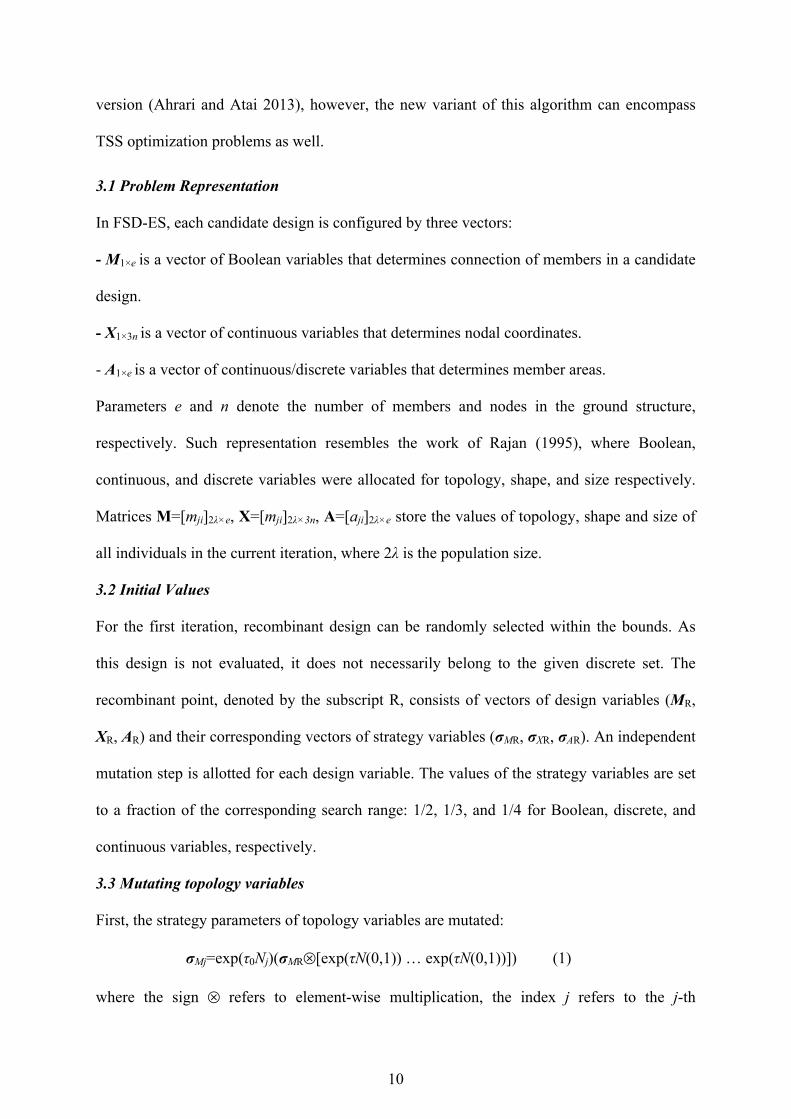
- For the 45-bar truss problem, FSD-ES can reach a structural weight of 44.000 lb after

19,656 function evaluations (FE), provided that the run is successful. 90% of

independent runs have converged to this weight and hence there is only a slight

difference between the ERT and FES for this problem. To the authors’ knowledge, the

best solution for this problem is 43.99 lb, reported by Wu and Tseng (2010), which

was reached after 30,800 evaluations. The best design of FSD-ES is quite similar to

25

theirs, but the required number of evaluations for the proposed FSD-ES is

comparatively smaller.

(a) (b)

(c) (d)

(e) (f)

Figure 3. ERT, SR and FES to reach arbitrary structural weights for the employed test problems: a) 45-bar truss,

b) 15-bar truss, c) 25-bar spatial truss, d) 39-bar truss, e) 47-bar truss and f) 68-bar truss.

0

0.2

0.4

0.6

0.8

1

7000

10000

13000

16000

19000

22000

44 49 54 59

SR ERT,FEs

W (lb)

45-bar

ERT

FEs

SR

0

0.2

0.4

0.6

0.8

1

1.E+03

1.E+04

1.E+05

1.E+06

69 72 75 78

SR ERT,FEs

W (Ib)

15-bar

ERT FEs SR

0

0.2

0.4

0.6

0.8

1

1.E+03

1.E+04

1.E+05

1.E+06

114 124 134

SR ERT,FEs

W (lb)

25-bar

ERT FEs SR

0

0.2

0.4

0.6

0.8

1

7.E+03

7.E+04

7.E+05

180 185 190 195

SR ERT,FEs

W (lb)

39-bar

ERT

FEs

SR

0

0.2

0.4

0.6

0.8

1

3.E+04

3.E+05

3.E+06

1845 1860 1875

SR ERT,FEs

W (lb)

47-bar

ERT

FEs

SR

0

0.2

0.4

0.6

0.8

1

8.E+04

8.E+05

8.E+06

1200 1350 1500

SR ERT,FEs

W (lb)

68-bar

ERT

FEs

SR

26

3

51

42

6

7

y

(a) (b)

(1)

(9)

(8)

(12)

(2) (3)

(11)

51

16

17

39

3 7

3632

34

6

yx

3x120=360

4x60=240

5x60=300

(1)(3)(5)(7)

(8) (6) (4) (2)

(9)(11)(13)

(14) (12) (10)

(15)

(17)

(19)

(21)

(22)

(20)

(18)

(16)

159

12

11

8

7

4

3

2610

15

16

14

13172125

31

33

35

29

39

30

36 38

2834

32

2624 20

23 19

4043 44 46 4745

1822

27

37

41 42

yx

(c) (d)

y

x (2)

(3)

(1)(4) (7)

(8)(5)

(6) (9) (12)

(10)

(11)(14)

(15) (18)(17)8

3 1119

28

38

4240322416

2

1 5

7

6

9 13

1510 182314

2126

25

31 34 39

17

(e)

Figure 4. The best final design for a) 45-bar truss b) 15-bar truss c) 39-bar truss d) 47-bar truss and e) 68-bar

truss problem.

- For the 15-bar truss problem, FSD-ES needs 3,859 FE to reach W=72.50 lb, however,

the ERT is more than five times larger. A rapid deterioration of SR starts at the target

weight of 75 lb, resulting in fast growth of the ERT. The best design found in this

study weighs 69.585 lb, and 5% of independent runs could reach W=70 lb after an

average of 8,508 FE. The best solution of SCPSO (Gholaizadeh 2013) weighs

W=72.49 lb and was reached after 12,500 FE, almost 4.2% heavier than the best

solution of the proposed FSD-ES. Moreover, SCPSO requires tuning of several

control parameters and selecting a grid. The best solution of FA (Miguel et al. 2013)

27

weighs 74.33 lb, reached after 8,000 FE. The GA proposed in Rahami et al. (2008)

reached the best solution of 75.10 lb after 8,000 FE, which is about 7.9% heavier than

the best solution found by the proposed FSD-ES. For this problem, FSD-ES surpasses

the best existing algorithms both in efficiency and quality of the best final solution.

- For the 25-bar spatial truss, FSD-ES requires on average 8,660 FE to reach W=114.42

lb, however, the corresponding SR is pretty low. To the authors’ knowledge, the best

reported solution for this problem is 114.36 lb (Rahami et al. 2008), reached after

10,000 FE. A GA by Tang et al. (2005) and FA by Miguel et al. (2013) could reach

W=114.74 lb and W=116.58 lb after 6,000 FE respectively. The best solution of

SCPSO (Gholaizadeh 2013) weighs 117.23 lb, reached after 8,000 FE. For this

problem, performance of FED-ES is quite similar to the best available results and

superior to SCPSO and FA.

- For the 39-bar truss problem, a gradual drop in SR initiates at W=190 lb, caused by

the existence of several topologically distinct high fitness designs at this zone.

However, 16% of independent runs could still reach W=182 lb, on average after

40,256 FE. For this problem, Luh and Lin (2008) reached W=188.73 lb after 453,600

FE, Luh and Lin (2011) reached W=188.86 lb after 262,500 FE, and Wu and Tseng

(2010) could reach W=188.45 lb after 137,200 FE. The FA of Miguel et al. (2013)

could reach W=191.30 lb after 50,000 FE. At the target weight of 188.0 lb, the FES

and ERT of FSD-ES are 20,686 and 26,185, spectacularly smaller than the number of

evaluations of the cited studies. The best feasible solution found in this study weighs

180.98 lb, which is about 3.7% lighter than and topologically different from the best

reported solution in the literature.

28

Table 5. The best solutions found for the test problems. Coordinates and areas are in inch and inch square,

respectively. The normalized constraint violation and the structure weight are provided in the four last rows. 45-bar truss 15-bar truss 25-bar truss 39-bar truss 47-bar truss 68-bar truss

A1 0.56569 x2=x6 100.0000 x4 38.8713 x8 53.9897 x2 100.9724 A11 0.9 x2 85.2171 x15 415.2320 A21 0.111 A2 0.56569 y2 135.1354 y4 61.5207 y8 151.2525 x4 80.4772 A13 2.7 y2 5.7523 y15 49.9535 A23 0.111 A3 0.44721 x3=x7 229.8186 z4 119.1785 x9 5.19128 y4 136.8699 A15 0.8 x4 119.1165 y17 40.0000 A24 2.142 A4 0.44721 y3 124.4261 x8 49.4146 y9 84.2778 x6 64.3908 A17 2.7 y4 -58.6499 x18 497.4523 A25 0.174 A5 0.18521 y6 -16.9664 y8 137.9423 y11 219.9569 y6 247.0491 A19 0.7 x5 175.0361 y18 56.8900 A26 0.111 A6 0.18521 y7 -9.2015 A1 - x12 172.0194 x8 55.2589 A21 2.5 y5 24.0102 A1 2.697 A28 2.697 A7 0.21479 y8 56.1693 A2 0.9 y12 210.2555 y8 338.4534 A23 0.9 x6 118.8412 A2 1.174 A31 0.111 A1 0.954 A3 0.1 A1 0.092396 x10 48.7333 A25 0.7 y6 64.7322 A3 3.565 A32 2.142 A2 0.539 A4 - A3 1.502843 y10 409.7380 A27 1.8 x7 243.4069 A5 0.539 A34 0.954 A4 0.954 A5 - A5 0.979807 x12 43.4742 A29 0.9 y7 -58.2763 A6 1.174 A38 2.697 A5 0.539 A6 1.0 A6 0.559607 y12 472.1479 A31 1.1 x8 243.8043 A7 1.174 A39 0.44 A6 0.44 A7 0.1 A7 0.823168 x14 44.8349 A33 0.3 y8 18.7154 A8 2.142 A40 1.764 A10 0.44 A8 0.1 A16 0.311426 y14 512.1901 A35 1 x9 209.0803 A9 0.287 A42 1.764 A11 0.44 A17 0.361835 x20 84.5040 A37 1.3 y9 59.7589 A10 0.954 A12 0.22 A32 1.215911 y20 630.3472 A39 0.9 x10 358.0904 A11 3.131 A13 0.22 A34 1.050755 x22 3.8414 A41 0.8 y10 -28.4162 A13 0.539

A14 0.44 A36 0.050055 y22 591.1449 A42 1.1 x11 400.2051 A14 0.44 A39 1.102177 A1 3.3 A43 0.1 y11 13.5412 A15 0.44 A3 1.1 A44 0.1 x12 302.6555 A16 1.764 A5 3.2 A45 0.1 y12 55.0556 A17 0.287 A7 1 A46 0.1 x14 477.8492 A18 0.44 A9 3 A47 0.1 y14 3.9185 A19 2.8

Stress 1.0000 1.0000 0.4490 1.0000 1.0000 1.0000 Buckling - - - - 1.0000 1.0000 Def. 0.6250 - 1.0000 0.7708 - 1.0000 Weight 44.000 lb 69.585 lb 114.417 lb 180.983 lb 1846.52 lb 1203.51 lb

- There are some notable points regarding this problem. First, several topologically

distinct high-fitness designs exist for this problem. In 100 independent runs, FSD-ES

converged to many distinct topologies. A number of these distinct final designs that

weigh less than 188 lb are illustrated in Figure 5. To the authors’ knowledge, only

topology #18 is reported in literature, meaning the previous algorithms couldn’t detect

topologies that potentially lead to lighter structures. Second, the best previously

reported designs have 13-15 active members, however, topologies that could reach

structures lighter than 187.5 lb generally have more members. This can pose a

challenge for truss optimizers that are biased toward simpler structures. Finally,

topologies of the best designs can hardly be guessed by engineering intuition, which

highlights benefits of using a reliable truss optimizer. Consequently, the proposed

29

FSD-ES significantly outperforms available optimizers for this problem, both in

efficiency and quality of the final designs.

- For the 47-bar truss problem, the best design, to the authors’ knowledge, weighs

1,861.1 lb (Gholaizadeh 2013), reached after 49,000 evaluations. However, the SR

was not reported and hence the ERT cannot be calculated. SA of Hasancebi and

Erbatur (2002b) could reach W=1,871.7 lb, but the FE was not reported. The best

solution of the proposed FSD-ES weighs 1,846.5 lb, relatively lighter than the best

available results. 86% of FSD-ES runs reached the target weight of 1861 lb, on

average after 55,802 FE. The convergence speed to reach this weight is quite similar

to that of SCPSO (Gholaizadeh 2013), but FSD-ES could produce a relatively lighter

structure.

 

(1)

(9)

(8)

(12)

(2) (3)(1)

(9)

(8)

(12)

(2) (3)

(11)

(1)

(9)

(8)(12)

(2) (3)

(11) (11)

(1)

(9)

(2) (3)

(12)

(1)

(9)

(8)

(12)

(2) (3)

(8)

(12)

(3)(2)(1)

(1)

(9)

(8)

(12)

(2) (3)

(11)

(1)

(8)

(11)

(2) (3)

(12)

(1)

(9)

(11)

(2) (3)

(12)

(8)

#2 #4

#7 #10#8

#18

#3

#13 #15Figure 5. Some selected final designs for the 39-bar truss problem which have distinct topology: Topology #2:

W=181.02 lb, Topology #3: W=181.38 lb, Topology #4: W=181.60 lb, Topology #7: W=182.37 lb, Topology

#8:W=183.34 lb, Topology #10: W=183.89 lb, Topology #13: W=186.91 lb, Topology #15: W=186.96 lb,

Topology #18: W=187.30 lb.

30

- For the 68-bar truss problem, independent runs of FSD-ES converged to a variety of

different designs ranging from 1,203.5 lb up to 1,555 lb. This is probably due to the

complexity of the ground structure and various reasonable topologies which may

challenge truss optimizers. The best final solution (Figure 4e) has a reasonable

topology where all three types of constraints were activated; however, no comparison

with other specialized algorithms can be made.

5 Summary and conclusions

Optimization of truss structures is a demanding task where problem complexity, prompted by

existence of various types of variables and constraints, require specialized variants of

optimization algorithms. In this article, an optimization algorithm based on evolution

strategies, called Fully Stressed Design based on Evolution Strategy (FSD-ES), was extended

to handle simultaneous topology, shape, and size truss optimization problems.

Based on the results of previous research on truss structure optimization, an

illuminative, discriminative and practically reasonable performance measure has been

employed to analyse, assess, and compare the obtained results. The calculation of the

Expected Running Time (ERT) has enabled us to not only compare efficiency of different

algorithms quantitatively, but also assess the short and long-term success of each algorithm.

Such statistical evaluation and presentation of results facilitate the comparison of

optimization algorithms, especially when the actual global minimum of the evaluated

problem is not known.

FSD-ES exhibited several advantages. First, unlike most available stochastic truss

optimizers that demand ad hoc tuning of several strategy parameters, FSD-ES is a quasi-

parameter-free method. In our experiments, all strategy parameters were set based on the a

priori known features of the problem. This makes the method a robust and practically useful

optimizer. Second, the proposed FSD-ES can be used for simultaneous optimization of

31

topology, shape, and size of truss structures. Third, in three test problems (15-bar, 39-bar, and

47-bar problems), the proposed FSD-ES method outperformed the best available solutions in

the literature. This is particularly true for the 39-bar truss, where it could detect several

topologically distinct designs that were lighter than the best available results in the

xliterature. For the 45-bar truss problem, the final solution of the existing best algorithms and

the proposed FSD-ES are quite similar, but FSD-ES converged relatively faster. For the 25-

bar spatial truss, the performance of FSD-ES is quite similar to the best available optimizers

when the final solutions and the required number of evaluations are compared. However, the

success rate when target weighs less than 117 lb are demanded is rather small, probably due

to the fact that the resizing step of FSD-ES focuses on the stress and buckling constraints

while only the deflection constraints were activated in this problem. The last problem was

introduced in this study as a significantly more complicated benchmark problem, especially

when considering that all three types of constraints were activated in the best final design.

Assessing and comparing prospective truss optimizers on this test problem provides

differentiating results in more complicated structures.

Based on the extensive results reported in this paper, the proposed methodology

seems to be an extremely competitive optimization algorithm. It is now ready to be applied to

more complex truss structure optimization problems involving topology, shape, and size

variables.

6 Acknowledgment

The authors would like to thank Matt Ryerkerk for his useful comments on this article.

32

References

Ahrari, A. and Atai, A.A., 2013. Fully Stressed Design Evolution Strategy for Shape and Size Optimization of

Truss Structures. Computers & Structures, 123, 58-67.

Auger, A., and Hansen, N., 2005. A restart CMA evolution strategy with increasing population size. The 2005

IEEE Congress on Evolutionary Computation, IEEE, 1769-1776.

Ayvaz, M.T., Kayhan, A.H., Ceylan, H. and Gurarslan, G., 2009. Hybridizing the harmony search algorithm

with a spreadsheet ‘solver’ for solving continuous engineering optimization problems. Engineering

Optimization, 41 (12), 1119-1144.

Bäck, T., Hammel, U. and Schwefel, H.P., 1997. Evolutionary computation: Comments on the history and

current state. Evolutionary computation, IEEE Transactions on, 1 (1), 3-17.

Beyer, H.G. and Schwefel, H.P., 2002. Evolution strategies–a comprehensive introduction. Natural computing,

1 (1), 3-52.

Beyer, H.G. and Sendhoff, B., 2008. Covariance matrix adaptation revisited–the CMSA evolution strategy.

Parallel problem solving from nature–PPSN X. Lecture Notes in Computer Science , 5199, 123-132.

Chen, T.Y. & Chen, H.C., 2006. “Discrete structural optimization by using evolution strategy”, 6th European

Solid Mechanics Conference ESMC 2006, Budapest, Hungary.

Chen, T.Y. and Huang, J.H., 2012. An efficient and practical approach to obtain a better optimum solution for

structural optimization. Engineering Optimization, 45 (8), 1005-1026.

Deb, K. and Gulati, S., 2001. Design of truss-structures for minimum weight using genetic algorithms. Finite

elements in analysis and design, 37 (5), 447-465.

Degertekin, S.O., 2011. Improved harmony search algorithms for sizing optimization of truss structures.

Computers & structures, 92–93, 229–41.

Ebenau, C., Rottschäfer, J. and Thierauf, G., 2005. An advanced evolutionary strategy with an adaptive penalty

functions for mixed-discrete structural optimisation. Advances in Engineering Software, 36 (1), 29-38.

Farajpour, I., 2011. A coordinate descent based method for geometry optimization of trusses. Advances in

Engineering Software, 42 (3), 64-75.

García, S., Molina, D., Lozano, M. and Herrera, F., 2009. A study on the use of non-parametric tests for

analyzing the evolutionary algorithms’ behaviour: A case study on the cec’2005 special session on real

parameter optimization. Journal of Heuristics, 15 (6), 617-644.

Gholizadeh, S., 2013. Layout optimization of truss structures by hybridizing cellular automata and particle

swarm optimization. Computers & Structures, 125, 86-99.

Hansen, N., 2009. Benchmarking a Bi-population CMA-ES on the BBOB-2009 function testbed. Proceedings of

the 11th Annual Conference Companion on Genetic and Evolutionary Computation Conference:

GECCO ‘09, 2389-2396.

Hansen, N., Auger, A., Finck, S. and Ros, R., 2010a. Real-parameter black-box optimization benchmarking

2009: Experimental setup. INRIA Research Report RR-6828.

Hansen, N., Auger, A., Ros, R., Finck, S. and Pošík, P., 2010b. Comparing results of 31 algorithms from the

black-box optimization benchmarking BBOB-2009. Proceedings of the 12th annual conference

companion on Genetic and evolutionary computation, GECCO’10, 1689-1696.

33

Hare, W., Nutini, J., and Tesfamariam, S., 2013. A survey of non-gradient optimization methods in structural

engineering. Advances in Engineering Software, 59, 19-28.

Hasançebi, O., 2007. Optimization of truss bridges within a specified design domain using evolution strategies.

Engineering Optimization, 39 (6), 737-756.

Hasançebi, O., 2008. Adaptive evolution strategies in structural optimization: Enhancing their computational

performance with applications to large-scale structures. Computers & Structures, 86 (1), 119-132.

Hasançebi, O., Çarbaş, S., Doğan, E., Erdal, F. and Saka, M.P., 2009. Performance evaluation of metaheuristic

search techniques in the optimum design of real size pin jointed structures. Computers & Structures, 87

(5), 284-302.

Hasançebi, O., and Erbatur, F., 2002a. Layout optimisation of trusses using simulated annealing. Advances in

Engineering Software, 33(7), 681-696.

Hasancebi, O., and Erbatur, F., 2002b. On efficient use of simulated annealing in complex structural

optimization problems. Acta Mechanica, 157 (1-4), 27-50.

Huang, X., and Xie, Y. M., 2007. Convergent and mesh-independent solutions for the bi-directional

evolutionary structural optimization method. Finite Elements in Analysis and Design, 43(14), 1039-

1049.

Hultman, M., 2010. Weight optimization of steel trusses by a genetic algorithm. M.Sc. Dissertation, Lund

University.

Kaveh, A., Farhmand Azar, B. and Talatahari, S., 2008. Ant colony optimization for design of space trusses.

International Journal of Space Structures, 23 (3), 167-181.

Kaveh, A. and Khayatazad, M., 2013. Ray optimization for size and shape optimization of truss structures.

Computers & Structures, 117, 82-94.

Kaveh, A. and Talatahari, S., 2009a. A particle swarm ant colony optimization for truss structures with discrete

variables. Journal of Constructional Steel Research, 65 (8), 1558-1568.

Kaveh, A. and Talatahari, S., 2009b. Size optimization of space trusses using big bang–big crunch algorithm.

Computers & structures, 87 (17), 1129-1140.

Kaveh, A. and Talatahari, S., 2010. Optimal design of skeletal structures via the charged system search

algorithm. Structural and Multidisciplinary Optimization, 41 (6), 893-911.

Kaveh, A. and Talatahari, S., 2011. An enhanced charged system search for configuration optimization using

the concept of fields of forces. Structural and Multidisciplinary Optimization, 43 (3), 339-351.

Kramer, O., 2010. “Evolutionary self-adaptation: A survey of operators and strategy parameters.” Evolutionary

Intelligence, 3 (2), 51-65.

Lagaros, N.D., Papadrakakis, M. and Kokossalakis, G., 2002. Structural optimization using evolutionary

algorithms. Computers & structures, 80 (7), 571-589.

Lamberti, L. and Pappalettere, C., 2011. Metaheuristic design optimization of skeletal structures: A review.

Computational Technology Reviews, 4, 1-32.

Lee, K.S., Geem, Z.W., Lee, S. and Bae, K., 2005. The harmony search heuristic algorithm for discrete

structural optimization. Engineering Optimization, 37 (7), 663-684.

34

Lee, K.S., Han, S.W. and Geem, Z.W., 2011. Discrete size and discrete-continuous configuration optimization

methods for truss structures using the harmony search algorithm. International Journal of

Optimization in Civil Engineering, 1, 107-126.

Li, L.J., Huang, Z.B., Liu, F. and Wu, Q.H., 2007. “A heuristic particle swarm optimizer for optimization of pin

connected structures. Computers & structures, 85 (7), 340-349.

Lu, Y., Jan, J., Hung, S. and Hung, G., 2012. Enhancing particle swarm optimization algorithm using two new

strategies for optimizing design of truss structures. Engineering Optimization,

DOI:10.1080/0305215X.2012.729054

Luh, G.C. and Lin, C.Y., 2008. Optimal design of truss structures using ant algorithm. Structural and

Multidisciplinary Optimization, 36 (4), 365-379.

Luh, G.C. and Lin, C.Y., 2011. Optimal design of truss-structures using particle swarm optimization.

Computers & Structures, 89 (23), 2221-2232.

Miguel, L.F.F., Lopez, R.H., and Miguel, L.F.F., 2013. Multimodal size, shape, and topology optimisation of

truss structures using the Firefly algorithm. Advances in Engineering Software, 56, 23-37.

Miguel, L.F.F., Miguel, L.F.F., 2012. Shape and size optimization of truss structures considering dynamic

constraints through modern metaheuristic algorithms. Expert Systems with Applications, 39 (10),

9458-9467.

Noilublao, N. and Bureerat, S., 2011. Simultaneous topology, shape and sizing optimisation of a three-

dimensional slender truss tower using multiobjective evolutionary algorithms. Computers & Structures.

89 (23–24), 2531–2538.

Papadrakakis, M., Lagaros, N.D., Thierauf, G. and Cai, J., 1998. Advanced solution methods in structural

optimization based on evolution strategies. Engineering Computations, 15 (1), 12-34.

Rahami, H., Kaveh, A., Aslani, M. and Asl, R.N., 2011. A hybrid modified genetic-Nelder mead simplex

algorithm for large-scale truss optimization. International Journal of Optimization in Civil

Engineering, 1, 29-46.

Rahami, H., Kaveh, A. and Gholipour, Y., 2008. Sizing, geometry and topology optimization of trusses via

force method and genetic algorithm. Engineering Structures, 30 (9), 2360-2369.

Rajan, S.D., 1995. Sizing, shape, and topology design optimization of trusses using genetic algorithm. Journal

of Structural Engineering, 121 (10), 1480-1487.

Reddy, G., and Cagan, J. 1993. Optimally directed truss topology generation using shape annealing. Technical

Report, Carnegie Mellon University.

Ros, R. and Hansen, N., 2008. A simple modification in cma-es achieving linear time and space complexity.

Parallel Problem Solving from Nature – PPSN X Lecture Notes in Computer Science , 5199, 296-305

Ruiyi, S., Liangjin, G. and Zijie, F., 2009. Truss Topology Optimization Using Genetic Algorithm with

Individual Identification. Proceedings of the world congress on engineering. Vol. 2, London..

Saka, M.P., 2003. Optimum design of skeletal structures: a review. Progress in civil and structural engineering

computing, 237-284.

Shea, K., and Cagan, J., 1999. The design of novel roof trusses with shape annealing: assessing the ability of a

computational method in aiding structural designers with varying design intent. Design Studies, 20(1),

3-23.

35

Shea, K., and Smith, I.F., 2006. Improving full-scale transmission tower design through topology and shape

optimization. Journal of structural engineering,132(5), 781-790.

Sonmez, M., 2011. Artificial bee colony algorithm for optimization of truss structures. Applied Soft Computing,

11 (2), 2406-2418.

Su, R., Wang, X., Gui, L. and Fan, Z., 2011. Multi-objective topology and sizing optimization of truss structures

based on adaptive multi-island search strategy. Structural and Multidisciplinary Optimization, 43 (2),

275-286.

Talatahari, S., Kaveh, A. and Sheikholeslami, R., 2012. Chaotic imperialist competitive algorithm for optimum

design of truss structures. Structural and Multidisciplinary Optimization, 46(3), 355-367.

Tang, W., Tong, L., and Gu, Y., 2005. Improved genetic algorithm for design optimization of truss structures

with sizing, shape and topology variables. International Journal for Numerical Methods in

Engineering, 62(13), 1737-1762.

Thierauf, G. and Cai, J., 1998. Parallelization of the evolution strategy for discrete structural optimization

problems. Computer-­‐Aided Civil and Infrastructure Engineering, 13 (1), 23-30.

Toğan, V. and Daloğlu, A.T., 2008. An improved genetic algorithm with initial population strategy and self-

adaptive member grouping. Computers & structures, 86 (11), 1204-1218.

Topping, B.H.V., 1983. Shape optimization of skeletal structures: A review. Journal of Structural Engineering,

109 (8), 1933-1951.

Wu, C.Y. and Tseng, K.Y., 2010. Truss structure optimization using adaptive multi-population differential

evolution. Structural and Multidisciplinary Optimization, 42 (4), 575-590.

Xie, Y.M. and Steven, G.P., 1993. A simple evolutionary procedure for structural optimization. Computers &

structures, 49(5), 885-896.