Pattern Recognition Letters 32 (2011) 1691–1700

Contents lists available at SciVerse ScienceDirect

Pattern Recognition Letters

journal homepage: www.elsevier .com/locate /patrec

Simultaneous estimation of vanishing points and their converging linesusing the EM algorithm

Marcos Nieto a,⇑, Luis Salgado b

a Vicomtech-ik4, Mikeletegi Pasealekua 57, 20009, San Sebastián, Spainb Grupo de Tratamiento de Imágenes, Universidad Politécnica de Madrid, Madrid, Spain

a r t i c l e i n f o a b s t r a c t

Article history:Received 6 September 2010Available online 22 August 2011Communicated by B. Kamgar-Parsi

Keywords:Vanishing pointsExpectation–MaximisationProjective planeMixture modelsNon-linear optimisation

0167-8655/$ - see front matter � 2011 Elsevier B.V. Adoi:10.1016/j.patrec.2011.07.018

⇑ Corresponding author. Tel.: +34 943 30 92 30; faxE-mail addresses: mnieto@vicomtech.org (M. Nie

(L. Salgado).

This paper introduces a new method for the simultaneous computation of sets of lines meeting at multi-ple vanishing points through the use of the Expectation–Maximisation (EM) algorithm. The proposedmethod is based on the formulation of novel error functions in the projective plane between lines andpoints which involve the use of non-linear optimisation procedures that allow to treat equally finiteand infinite vanishing points. These functions are included into the EM framework, which handles themulti-modality of the problem naturally with mixture models. Results show that the proposed methodof joint computation of vanishing points and lines converging at such points enhances the robustnessand the accuracy of locating these points.

� 2011 Elsevier B.V. All rights reserved.

1. Introduction

Vanishing points are elements of great interest in the computervision field. They are the main source of information about struc-tured environments in images. A vanishing point is a point in theimage to which parallel lines of the scenario appear to converge.Their importance lies in their correspondence to three-dimensionaldirections in the space. Hence, they can be used to retrieve informa-tion about the camera projection parameters or the geometry of thescene. There are a number of applications that can take advantage ofthe computation of these points, such as plane rectification(Liebowitz and Zisserman, 1998), camera calibration (Wang et al.,2009), single view metrology (Criminisi et al., 2000), compass esti-mation (Coughlan and Yuille, 1999), and others. Besides, some ofthese applications require the computation of lines meeting atvanishing points. For instance, Schaffalitzky and Zisserman (2000)have shown that the detection of imaged lines meeting at a commonvanishing point, that actually correspond to equally spaced parallellines in the scene, can be used to retrieve the line at the infinity.Other authors, like Trinh and Jo (2006), have used lines meeting atvanishing points to estimate the volume of buildings, or to estimatethe geometry of road lanes in traffic applications like Rasmussen(2004) or Lai and Yung (2000). The estimation of vanishing pointsin images has been studied by the computer vision research commu-nity for decades, yielding a very significant number of noteworthy

ll rights reserved.

: +34 943 30 92 93.to), L.Salgado@gti.ssr.upm.es

works (Almansa et al., 2003; Barnard, 1983; Košecká and Zhang,2003; Liebowitz, 2001; Lutton et al., 1994; McLean and Koyyuri,1995; Pflugfelder, 2008; Schindler and Dellaert, 2004). Althoughmost of these works compute vanishing points through optimisationprocedures, lines are typically obtained with additional processingsteps such as the Hough transform. Therefore these works do notoffer a closed solution for both problems and the combination of dif-ferent nature methods does not offer the robustness and reliabilityof a joint optimisation procedure. In this paper a new method forcalculating multiple vanishing points is introduced based on theEM algorithm. The major contribution of this work is the definitionof a closed solution in the projective plane for the simultaneousestimation of vanishing points and the most significant lines thatconverge in those vanishing points by means of the introduction ofa mixture model into the EM algorithm. The estimation of theseelements in a single optimisation framework offers excellent esti-mation results, in terms of accuracy and robustness, improving theresults of approaches that do not consider lines within their models.This paper is structured as follows: Section 2 summarises the litera-ture related to vanishing point estimation to clarify the contributionof our work. Section 3 defines the proposed likelihood models aswell as the required data calibration and normalisation stages. Sec-tion 4 describes the proposed steps of the EM algorithm, and Section5 presents a performance evaluation and the obtained results.

2. Related work

The following subsections describe and classify the most relevantvanishing point estimation methods according to their workspace,

1692 M. Nieto, L. Salgado / Pattern Recognition Letters 32 (2011) 1691–1700

the estimation technique used and the number of detected vanish-ing points. Table 1 summarises the most relevant properties of thesemethods.

2.1. Workspace

Vanishing points can be described mathematically in differentways. On the one hand, points are 2D image entities but on theother hand they correspond to 3D space directions. Therefore, wecarry out a first classification of vanishing point detection tech-niques according to the workspace they use and associated param-eterisation of vanishing points. Some authors have chosen theimage plane itself as workspace such as Caprile and Torre (1990),McLean and Koyyuri (1995), Sekita (1994) and more recentlyMinagawa et al. (2000) and Suttorp and Bücher (2006). For in-stance, Suttorp and Bücher (2006) estimates the position of themain vanishing point under the assumption that in road scenes ittypically lies inside the limits of the image and, therefore, theimage plane can be then used as the workspace. Not restricted toone single vanishing point, other authors such as McLean andKoyyuri (1995), Sekita (1994) or Minagawa et al. (2000) define er-ror measurements on the image plane to optimally estimate theposition of several vanishing points. Specifically, Minagawa et al.(2000) propose as error measurement the normal distancebetween the vanishing points and the lines that contain the linesegments. Barnard (1983) proposed to project the image plane,which is by definition an unbounded space, on a unit sphere cen-tered at the optical center of the camera. The target is to work witha bounded space on which operations are simplified and thus finiteand infinite vanishing points are treated equally. Most of subse-quent works (Magee and Aggarwal, 1984; Quan and Mohr, 1989;Lutton et al., 1994) made explicit use of the unit sphere using itssurface, properly tessellated, as the accumulation space where tosearch for maxima that determine the presence of dominant van-ishing points. As an alternative to the image plane, and as a math-ematical formalisation of the unit sphere parameterisation, otherworks emerged that use the projective plane to analytically handleinfinite points in a natural way (Liebowitz, 2001; Pflugfelder, 2008;Rother, 2000). Analogously to the unit sphere, this search requiresto augment the dimension of vanishing points by adopting the useof homogeneous coordinates. These works overcome the draw-backs of accumulation processes on the unit sphere by proposingerror functions between vanishing points and image features thatdo not depend on the position of the vanishing point, and alsoapplying optimisation techniques such as RANSAC or EM (Košecká

Table 1Classification of vanishing point estimation methods.

Ref. Year Workspace C

Barnard (1983) 1983 Sphere HMagee and Aggarwal (1984) 1984 Sphere SQuan and Mohr (1989) 1989 Sphere HCaprile and Torre (1990) 1990 Image plane VLutton et al. (1994) 1994 Sphere SMcLean and Koyyuri (1995) 1995 Image plane CTuytelaars et al. (1998) 1998 Hough CAntone and Teller (2000) 2000 Sphere EMinagawa et al. (2000) 2000 Image plane ERibeiro and Hancock (2000) 2000 Sphere SRother (2000) 2000 Image plane MCantoni et al. (2001) 2001 Hough/image plane VLiebowitz (2001) 2001 Projective plane OKošecká and Zhang (2003) 2003 Unc. Sphere EAlmansa et al. (2003) 2003 Image plane ESchindler and Dellaert (2004) 2004 Projective plane ESeo et al. (2006) 2006 ICIS InPflugfelder (2008) 2008 Projective plane O

LSegs.: Line segments; Vps.: Vanishing points; Vl.: Vanishing line; -: Unknown or unspe

and Zhang, 2003; Antone and Teller, 2000). Other authors proposedalternative transformed spaces to handle vanishing points at infin-ity (Cantoni et al., 2001; Seo et al., 2006; Tuytelaars et al., 1998).Tuytelaars et al. (1998) defined an intelligent partition of the para-metric line space (computed as the Hough transform) by consider-ing three bounded sub-spaces that were used to detect vanishingpoints and also vanishing lines. Similar approaches were proposedby Almansa et al. (2003) and Seo et al. (2006). The work by Cantoniet al. (2001) focused on the polar space obtained as the polarHough transform of the points on the image. In this space, vanish-ing points at infinity are represented as sinusoids which areestimated through linear least squares optimisation.

2.2. Type of approach

Vanishing point estimation strategies are typically composed oftwo fundamental steps named clustering and estimation. The for-mer classifies the image features into groups, or clusters, that sharea common vanishing point; the latter considers the information ofthe cluster and estimates the position of the vanishing point. Manyauthors have converged to the use of iterative joint strategies,which contain the grouping and estimation stages as an alternatingprocess. Specifically, the most used techniques are those based onrobust estimation tools, such as RANSAC or its variants, and opti-misation strategies based on mixture models using the EM algo-rithm. The methods based on RANSAC (RANdom Sampling AndConsensus) (Pflugfelder, 2008; Rother, 2000) work iterativelyselecting a minimal sample set of image features, which is usedto compute a candidate vanishing point, and then finding the setof features that are coherent with it. Once this consensus set hasbeen determined, the vanishing point can be re-estimated usingthe information of the elements of the whole consensus set. Todetermine more vanishing points, the features already used tocompute the vanishing point are removed and the RANSAC itera-tions are restarted to search for a new vanishing point Pflugfelder(2008). The procedure is repeated until there are not enough fea-tures to determine new vanishing points. The EM (Expectation–Maximisation) algorithm has been shown to be a very powerfultool for recursive estimation and clusterisation. As opposed toRANSAC, EM allows to assign each line segment to different vanish-ing points with particular probabilities. The iterative process runsuntil the position of all vanishing points has been determined(Antone and Teller, 2000; Košecká and Zhang, 2003; Minagawaet al., 2000; Pflugfelder, 2008; Sekita, 1994). Typically, these meth-ods are devised and used to refine results obtained with faster

ontribution Num. Vps. Lines

ough accumulation on sphere surface 3 Noearch for clusters of intersections. – Noierarchical Hough transform – Nops. matching – Noemi-regular sphere quantification 3 orth. Noluster and estimate approach 1 Noascaded Hough transform N and Vls. YesM algorithm, angle error model N NoM algorithm for lines and Vps. and Vl. N and Vl. Yespectral voting and search for maxima N Noid-point error model, unbounded search 3 No

oting and least squares sinusoid 1 Noptimal MLE solution for LSegs. 1 NoM algorithm, outliers control and refinement N Noquiprobable vanishing regions N NoM algorithm, Atlanta world N Noverted Coordinate Image Space N Nonline scheme with EM algorithm N No

cified; Unc.: Uncalibrated.

M. Nieto, L. Salgado / Pattern Recognition Letters 32 (2011) 1691–1700 1693

approaches such as RANSAC, thus providing very accurate resultsalthough at the cost of significantly increasing the computationalrequirements. The work by Schindler and Dellaert (2004) is note-worthy as it uses the EM algorithm with on–off mixture modelsfor edge points on the projective plane. Additionally, as opposedto many works that search for three vanishing points that corre-spond to the three orthogonal directions of the Euclidean space(Lutton et al., 1994; Quan and Mohr, 1989; Rother, 2000) (typicallyknown as Manhattan worlds (Coughlan and Yuille, 1999)), thiswork does not require additional information from the scenario(known as Atlanta world).

2.3. Number of vanishing points and lines

The number of vanishing points obtained by each approach isstrongly related to their use. For instance, methods that computevanishing points for camera autocalibration need at least threevanishing points, while those for plane rectification just requiretwo. There are methods that fit models assuming the existence ofa single vanishing point (Cantoni et al., 2001; Liebowitz, 2001;McLean and Koyyuri, 1995), although they can be used to obtainseveral vanishing points (i.e. the image features used to computethe first vanishing point are removed from the feature set to com-pute the next vanishing point). However, other approaches doactually consider multiple vanishing points in their models so thatthey are computed simultaneously (Antone and Teller, 2000;Košecká and Zhang, 2003; Minagawa et al., 2000; Schindler andDellaert, 2004; Seo et al., 2006; Tuytelaars et al., 1998).

2.4. Comparison with other joint strategies

Nevertheless, only few works do actually assume that vanishingpoints are the intersection of dominant lines meeting at them andcompute the parameters of these lines. For instance, Tuytelaarset al. (1998) proposed a cascade of Hough transforms to identifylines as dominant clusters of edge points, vanishing points as theirintersection, and finally vanishing lines. The use of the EM algo-rithm for this purpose was introduced by Minagawa et al. (2000),which defined a solution in the image plane for the simultaneousestimation of clusters of lines and their vanishing points. Neverthe-less, in contrast to our proposal, it can not treat properly vanishingpoints far from the image, and it proposes a limited model toobtain a linear solution: only the position of the edge points ismodeled within the EM algorithm and no solution to handle outli-ers is considered.

(a)

(b)Fig. 1. Relative orientation h between the orientation of the measured feature andthe line that joins the vanishing point v and the feature ((a) line segments and (b)edge-points). When the vanishing point lies on l the error is minimum.

3. Projective-plane solution

This section describes in detail the workspace of the proposedapproach, including concepts related to the projective plane suchas data normalisation and likelihood models definition. These con-cepts are further used in the description of the proposed EM algo-rithm described in Section 4.

3.1. Image features

The input image information required for vanishing point esti-mation can be any feature with orientation, such as gradient-pixels(pixels with enough gradient magnitude) or line segments. Thesefeatures are equivalent since they can be both expressed as a linein homogeneous coordinates (this concept is illustrated in Fig. 1).Let r = (x,y,1)> be the homogeneous coordinates of a point of theimage plane with significant gradient magnitude defined by thecomponents of the gradient vector g = (gx,gy)>. Any such gradi-ent-pixel can be expressed as a line l = r � (r + km), where m is

the normal to the gradient vector, and k is any real number.Besides, a line segment is defined by a pair of end-points {a,b} suchthat they define the line l = a � b = (l1, l2, l3)> in homogeneous coor-dinates. Its associated reference point is the mid-point c ¼ aþb

2 . As ageneralisation, let us consider from here on a data sample as theset x = {r, l}, whose elements are derived either from a gradient-pixel or a line segment (in this latter case, let use a common nota-tion for the reference point: c = r).

3.2. Data calibration and normalisation

Each data sample on the image plane defines a plane that passesthrough the optical center of the camera model. This plane isdenominated ‘‘Edge Plane’’ by Antone and Teller (2000), althoughit is more frequently identified as the ‘‘Interpretation plane’’ asdone by Pflugfelder (2008). This plane intersects a sphere centeredas well at the optical center generating the so-called ‘‘great circles’’.The intersections between these circles correspond to the intersec-tion of the corresponding lines on the image plane. Fig. 2 illustratesthese concepts. An interesting property we get from these defini-tions is that a vanishing point can be treated as a 3D direction,instead of just as a 2D point on an image. The vanishing directionis defined by the vector that joins the optical center and the pointon the surface of the sphere which is the intersection of two ormore great circles that correspond to lines meeting at a commonvanishing point. Vanishing points are represented in homogeneouscoordinates as v = (v1,v2,v3)> (Hartley and Zisserman, 2004). Thisrepresentation allows handling projective relationships with linearmatrix operations. For instance, the projection of a point in thespace X = (X,Y,Z,1)> into the image plane is:

xhom ¼ K½Ij0�X ð1Þ

where K is the camera calibration matrix, I is the identity 3 � 3 ma-trix, and 0 is a column 3 � 1 vector of zeros. The image coordinatesof this projected point are then obtained by dividing xhom by itsthird coordinate, obtaining the inhomogeneous coordinates of thepoint in the image plane xinh ¼ f X

Z ; fYZ

� �>. One dimension is lost pro-jecting a space point onto the image plane since any point lying onthe ray that joins X with the optical center C is projected in the sameimage point (Hartley and Zisserman, 2004). From a geometric pointof view, if the camera calibration matrix is known, the aforemen-tioned ray can be retrieved from any 2D image point. For the case

Zv

v’

C

Y

XParallel 3D lines

Unit sphere projection

Image plane

Fig. 2. Two parallel 3D lines are projected onto the image plane meeting at thevanishing point v. Its calibrated and normalised version v0 can be seen either as theray joining the optical center C and v or as the intersection of the two great circlesdefined by the projected lines.

1694 M. Nieto, L. Salgado / Pattern Recognition Letters 32 (2011) 1691–1700

of a vanishing point, this ray actually corresponds to the 3D direc-tion of the parallel lines in the 3D world. Indeed, when parallel linesare projected onto the image they converge at a vanishing point.This idea is illustrated in Fig. 2. To explain this concept, let us sup-pose that there are two parallel lines in the 3D world whose com-mon director vector is D = (X,Y,Z)>. The intersection of these linesis at some point in the infinity that we can represent in homoge-neous coordinates as V = (X,Y,Z,0)>. This point is projected as thevanishing point v = K[Ij0]V. If we left-multiply both members of thisexpression by K�1 we obtain K�1v = [Ij0]V = (X,Y,Z)>, which rendersa new 3D vector v0 = K�1v. We will refer to this transformation as‘‘data calibration’’ as other authors do (Košecká and Zhang(2003)). Hence, the calibration of a vanishing point yields the actual3D direction of the parallel lines whose projections onto the imageplane converge at it. This transformation can also be understood asthe transformation of the 2D coordinates of the image features(points and lines) into the 3D coordinates under the camera coordi-nate system. Data calibration is carried out in the following way:points are normalised with K�1 as x0 = K�1x and lines with K> asl0 = K>l. Besides, to be able to represent these elements on the unitsphere, an additional scale normalisation must be applied such thatthe norm of the 3D vectors is the unity. When the camera calibra-tion is not available working with the homogeneous vector v entailsan implicit distortion in the angular information. For instance, thecosine of the angle between two uncalibrated directions is depen-dent on an unknown distortion given by x = K�>K�1:

cos a ¼ v 0>1 v 02kv 01kkv 02k

¼ v>1 xv2ffiffiffiffiffiffiffiffiffiffiffiffiffiffiffiffiv>1 xv1

p ffiffiffiffiffiffiffiffiffiffiffiffiffiffiffiffiv>2 xv2

p ð2Þ

Nevertheless, the camera calibration matrix can be easilyapproximated by a default projective transformation based onthe image dimensions, which reduces the aforementioned inherentdistortion, as done by some authors (Košecká and Zhang (2003)):

eK ¼ W 0 W=20 H H=20 0 1

0B@1CA ð3Þ

where W and H are the width and height of the image in pixels,respectively.

3.3. Likelihood models

Given a data set X ¼ fxigNi¼1, vanishing point estimation tech-

niques typically focus on only the optimisation of the parametersof the vanishing point v (or the set of vanishing points). In ourapproach the dimensionality of the problem is augmented sincethe set of parameters to be optimised is now given by a set of van-ishing points fvkgV

k¼1 and a set of supporting or main lines that passthrough them fsjkgM;V

j¼1;k¼1. Let us define the relationship between

data samples and the set of supporting lines. The likelihood modelis governed by two equations that link each data sample xi = {ri, li}with lines meeting at a common vanishing point (the subindex khas been removed for the sake of clarity), fsjgM

j¼1, as:

pðxijsjÞ ¼ pðrijsjÞpðlijsjÞ ð4Þ

where the point-line and line-line distances are given by three-vec-tor dot products:

pðrijsjÞ / exp � 12r2

q;jr>i sj� �2

!ð5Þ

pðlijsjÞ / exp � 12r2

/;j

1� l>i sj

� �2� � !

ð6Þ

Fig. 3 illustrates these functions. The point-line distance, r>i sj in(5) assumes that vectors are normalised such that krik = ksjk = 1.Therefore, this distance corresponds to the cosine of the angle de-fined by the vector that joins the optical center C with the point ri

and the normal vector of the plane defined by the great circle thatcorresponds to the line sj. This way, if the point belongs to the lineon the image plane, its associated 3D vector is orthogonal to thenormal vector of the interpretation plane and (5) is maximum.The line–line distance, considering also normalised vectors, is re-lated to the sine of the angle between the interpretation planescorresponding to li and sj. Particularly, given that cosðhÞ ¼ l>i sj

� �and sin2(h) = (1 � cos2(h)) then sin2ðhÞ ¼ 1� l>i sj

� �2. Therefore, if

the lines are equal, these normal vectors are coincident and thesine of their angle is zero so that the likelihood as in (6) is maxi-mum. The result is a likelihood function defined by a mixture mod-el of M supporting lines grouped in V sets that correspond todifferent vanishing points in the scene plus an additional compo-nent that handles outliers:

pðxijH;XÞ ¼XV

k¼1

XM

j¼1

xjkpðxijhjkÞ þxoutpoutðxiÞ ð7Þ

where H ¼ fhjkgM;Vj¼1;k¼1 and hjk = {sjk,r/,jk,rq,jk}, and the mixture

model components are X ¼ fxjkgM;Vj¼1;k¼1;xout

n o. This expression

already includes a component of the mixture devoted to outlierssuch that the weights sum to one:

XV

k¼1

XM

j¼1

xjk

!þxout ¼ 1 ð8Þ

The outlier distribution can be defined as a normal distributionwith fixed large variance which approximately behaves as a uni-form distribution. The use of such a normal distribution has beenalready addressed by other authors like Košecká and Zhang(2003). The reason of choosing this approximation instead of theuniform itself is because the EM algorithm for a mixture of Gaussi-ans is much simpler to compute. Note that, although the standarddeviation of the supporting lines could be different according tothe indexes j and k, we will consider, for the sake of simplicity, thatthere is a common value r/,jk = r/ and rq,jk = rq "j = 1 . . .M,k = 1 . . .V. The presence of multiple i.i.d. data samples yields theincomplete likelihood function pðXjHÞ ¼

QNi¼1pðxijH;XÞ, and the

log-likelihood function which includes the summation on clustersof lines indexed by k:

logLðHjXÞ ¼XN

i¼1

logXV

k¼1

XM

j¼1

xjkpðxijhjkÞ þxoutpoutðxiÞ !

ð9Þ

Given the definition of the likelihood model for data samplesand supporting lines let us now consider the relationship betweenvanishing points and data samples. For this purpose, we could useany error function, like the calibrated point-line distance l>i v . This

Z

sj

ri

C

Y

Xr’i

s’jZ

sj

li

C

Y

X

l’i s’j

(a) (b)Fig. 3. Point–line and line–line distances in the projective plane. The unit sphere visualisation helps to understand the proposed distances as relationships between vectorsjoining the optical center, C, and points in the surface of the sphere. For clarity, in this figure, calibrated coordinates are depicted with a tilde.

M. Nieto, L. Salgado / Pattern Recognition Letters 32 (2011) 1691–1700 1695

distance is equivalent to the point-line distance s>j ri that was illus-trated in Fig. 3. Nevertheless, it has been shown Nieto and Salgado(2010) that more accurate results can be found using the orienta-tion deviation between li and a line joining the vanishing pointand a reference point, which is the mid-point of the line segment.

dðx;vÞ ¼ j sinðhÞj ¼ j � l2s1 þ l1s2jffiffiffiffiffiffiffiffiffiffiffiffiffil21 þ l22

q ffiffiffiffiffiffiffiffiffiffiffiffiffiffis2

1 þ s22

q ð10Þ

This distance represents the error between a vanishing point vin homogeneous coordinates and the orientation of the data sam-ple x. It is related to the absolute value of the sine of the angle hbetween l and a line s = (s1,s2,s3)> that joins v and r (as shown inFig. 1) and that can be computed as s = v � r. It is important to rea-lise that this error function is defined on uncalibrated coordinates.Hence, in this case, data has not to be calibrated. The likelihood of adata sample xi to belong to a vanishing point v is given by

pðxijvÞ / exp � 12r2 d2ðxi;vÞ

� �ð11Þ

where d(xi,v) is defined as in Eq. (10).

4. EM algorithm

The EM procedure can be described once we have defined thelikelihood models. The process has to be done gradually, i.e. withseveral M-steps and, for this case, also several E-steps since thereis not a single expression to update at once all the model parame-ters. The following paragraphs summarise the proposed way toproceed, which updates in the first M-step the position of the van-ishing points fvkgV

k¼1 and in the second one the parameters of thesupporting lines fsjkgM;V

j¼1;k¼1. Although it is possible to proceed theother way round, i.e. updating first the parameters of the support-ing lines and then the position of the vanishing points, empiricaltests have shown that this approach is more prone to errors.Updating the vanishing point position first allows the E-step toclassify data samples according to the vanishing point they meetand then update the supporting lines.

4.1. E-step (1)

This step computes the conditional probabilities of the set ofdata samples with respect to the set of vanishing points and theircorresponding supporting lines. Given the current best estimationof the parameters of the model H⁄ and X⁄ these probabilities arecomputed as

pðj; kjxi;H�Þ ¼

x�jkpðxijh�jkÞ

xoutpoutðxiÞ þPV ;M

k0 ;j0¼1

x�j0k0

pðxijh�j0k0 Þð12Þ

where pðxijh�jkÞ is computed as defined in (4). For the sake of simplic-ity, p(j,kjxi,H⁄) will be denoted as cijk from here on.

4.2. M-step (1)

Once the conditional probabilities have been computed, the firstmaximisation step estimates the position of the set of vanishingpoints minimising the selected error function. In case of usingthe error function in uncalibrated coordinates, defined in Eq.(10), the conditional probabilities cik can be used as the scale factorso that the error function is redefined as d0(x,v) = cikd(x,v). Notethat the index j has disappeared from cijk as for the estimation ofeach vanishing point the dimension corresponding to the support-ing lines is marginalised. The set of data samples is classifiedaccording to cik, i.e. according to the vanishing point they mostlikely belong. Then, for each vanishing point vk and its correspond-ing subset of samples X k the function to be minimised is

logLðvkjX kÞ ¼X

xi2Xk

d2ðxi;vkÞ ð13Þ

which can be solved with the Levenberg–Marquardt algorithm thatupdates the vanishing point vk. The initialisation of this procedurecan be random, although we have found better results if the initiali-sation is carried out using the calibrated point-line minimisation.This is a linear approach that can be solved in a least squares sense:as a linear optimisation problem, the least squares solution for eachvk is the eigenvector with smallest eigenvalue of the problem(Košecká and Zhang, 2003)

L>C>CL� �

vk ¼ kvk ð14Þ

where L is a N � 3 matrix, in which each row corresponds to thedata sample li in row format, and C is a N � N diagonal matrix ofweights that corresponds to the conditional probabilities cik.

4.3. M-step (2)

After M-step (1), as the position of the vanishing points havebeen updated, it is required to re-compute the parameters of theirsupporting lines so that they meet at their new positions. This con-cept is illustrated in Fig. 4. The problem is stated for each support-ing line sjk as

sjk ¼ argmaxs�

jk

s>jks�jk� �2

subject to s>jkvk ¼ 0 ð15Þ

The solution to this problem can be found using iterative meth-ods for non-linear minimisation with restrictions. For instance, asequential quadratic programming (SQP) method has been used.

v

v*

s1*

s2*

s2

s1

Fig. 4. Given the new position of the vanishing point, v, the lines s�1 and s�2 are re-estimated yielding s1 and s2 such that they actually pass through v and the angulardistances s>j s�j are minimised.

100 200 300 400 500 600

0

50

100

150

200

250

300

350

400

450

Fig. 5. Line segments obtained with the automatic line segment detector. Thecolour code indicates the classification of the segments according to the vanishingpoint they most likely belong to according to the RANSAC method.

1696 M. Nieto, L. Salgado / Pattern Recognition Letters 32 (2011) 1691–1700

4.4. E-step (2)

After the re-estimation of the supporting lines the conditionalprobabilities have to be updated according to the new parametersof the supporting lines. Therefore, the values of cijk are re-computedas in (12).

4.5. M-step (3)

Finally, using the updated conditional probabilities and the like-lihood function defined in (9), the parameters of the set of support-ing lines have to be updated. The problem to be solved for each linesjk is defined as:

sjk ¼ argmaxs�

jk

logLðHjXÞ ð16Þ

subject to s>jkvk ¼ 0 and ksjk = 1k. This problem can be againsolved using iterative methods for non-linear minimisation withrestrictions as in M-step (2).

5. Testing and discussion

In this section we present several tests that evaluate differentaspects of the proposed method. We use the York Urban Data Base(YUDB) (Denis et al., 2008), which contains a set of 102 images ofstructured environments including ground truth vanishing pointsand line segments with available camera calibration information.First, we analyse the dependency of the proposed EM algorithmwith respect to the initialisation of the vanishing points. Second,we compare two different approaches for automatic initialisation:a RANSAC-based method Nieto and Salgado (2010) and a variationof the Hough transform proposed by Almansa et al. (2003). Finally,we present the results of the execution of the proposed strategy onthe set of images of the YUDB. For the tests, we have used two dif-ferent input data sources: (i) the ground truth line segments of theYUDB, which contain no outliers (i.e. line segments that do notmeet any vanishing point); and (ii) automatically computed linesegments using the SSWMS algorithm Nieto et al. (2011), whichrenders relevant segments in the image, regardless if they meetor not at any vanishing point. This algorithm is fast (can be usedin online applications) and yields accurate line segments whilekeeping a low false alarm ratio. Fig. 5 shows an example of the linesegments computed using this method.

5.1. Initialisation analysis

The described EM method requires initialisation of the targetparameters: the vanishing points and their corresponding support-ing lines. As described in the literature Minagawa et al. (2000), EM

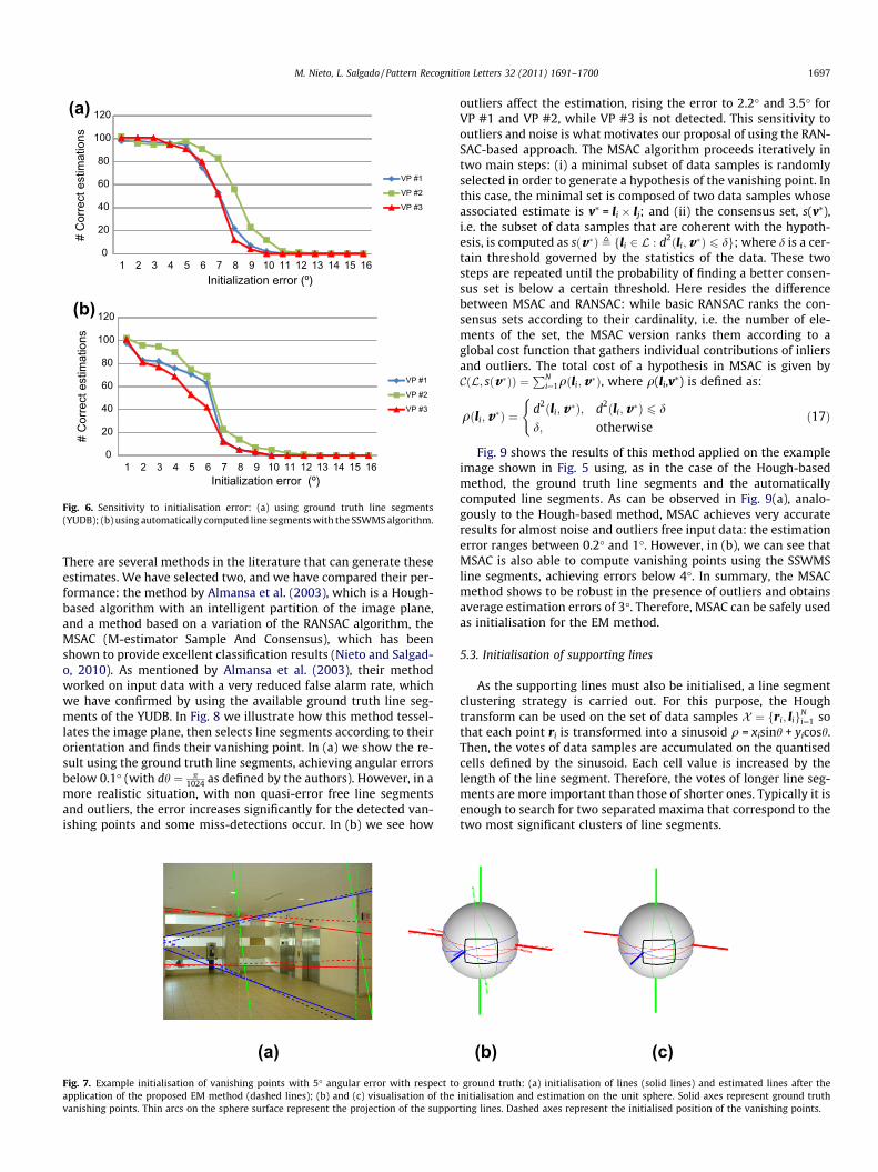
based strategies are quite sensitive to the initialisation process:they are able to compensate errors in the initialised target param-eters up to certain deviation from their actual values. Therefore,any initialisation procedure should take this constraint intoaccount to reach the desired results. To evaluate the sensitivityof the proposed strategy we have executed the EM method for allthe images of the YUDB using as initialisation vanishing pointswith increasing angular error in their position (since they can betreated as 3D vectors, the error between two vanishing pointscan be computed as an angle, as described in Eq. (2)). Angularerrors between 1� and 15� have been used for the analysis,although it should be noticed that errors above 5� are in manycases too severe, and they are particularly relevant for vanishingpoints close to the image frame. The results of the test are illus-trated in Fig. 6. In (a) the results correspond to the execution ofthe proposed method using ground truth line segments while (b)shows the results obtained using the SSWMS line segments. Eachfigure shows three curves, each one corresponding to one of thethree vanishing points of the images according to the YUDB crite-rion Denis et al. (2008) (VP #1 is the most significant horizontalvanishing point, VP #2 is the vertical vanishing point, and VP #3is the second most significant vanishing point). These curves depictthe number of images for which the EM method has found the cor-rect solution, i.e. reaching estimates of the vanishing points closeto the ground truth. Using ground truth line segments, the pro-posed method shows excellent results (above 90%) for deviationsup to 6�, with slightly better results for VP #2 as it is the verticalvanishing point and it is typically supported by more line segmentsthan the other vanishing points (an example is shown in Fig. 7). Asexpected, the performance decreases when the SSWMS segmentsare used: the main reason is the presence of clutter or outliers,i.e. line segments not meeting at any of the ground truth vanishingpoints. When the initialisation error increases, the clutter can moreeasily drive the estimation to local minima and thus make the sys-tem fail to find the correct vanishing points. The figures show thatthe best performance corresponds to the estimation of the VP #2,while VP #3 is more sensitive to the clutter, as it is the vanishingpoint located typically near or inside the limits of the image frame.

5.2. Automatic initialisation of vanishing points

As noted in the previous subsection, the EM method needs ini-tializations with relatively low error (up to 5� approximately).

0

20

40

60

80

100

120

1 2 3 4 5 6 7 8 9 10 11 12 13 14 15 16

# C

orre

ct e

stim

atio

ns

VP #1

VP #2

VP #3

Initialization error (º)

(a)

0

20

40

60

80

100

120

1 2 3 4 5 6 7 8 9 10 11 12 13 14 15 16

# C

orre

ct e

stim

atio

ns

VP #1

VP #2

VP #3

Initialization error (º)

(b)

Fig. 6. Sensitivity to initialisation error: (a) using ground truth line segments(YUDB); (b) using automatically computed line segments with the SSWMS algorithm.

M. Nieto, L. Salgado / Pattern Recognition Letters 32 (2011) 1691–1700 1697

There are several methods in the literature that can generate theseestimates. We have selected two, and we have compared their per-formance: the method by Almansa et al. (2003), which is a Hough-based algorithm with an intelligent partition of the image plane,and a method based on a variation of the RANSAC algorithm, theMSAC (M-estimator Sample And Consensus), which has beenshown to provide excellent classification results (Nieto and Salgad-o, 2010). As mentioned by Almansa et al. (2003), their methodworked on input data with a very reduced false alarm rate, whichwe have confirmed by using the available ground truth line seg-ments of the YUDB. In Fig. 8 we illustrate how this method tessel-lates the image plane, then selects line segments according to theirorientation and finds their vanishing point. In (a) we show the re-sult using the ground truth line segments, achieving angular errorsbelow 0.1� (with dh ¼ p

1024 as defined by the authors). However, in amore realistic situation, with non quasi-error free line segmentsand outliers, the error increases significantly for the detected van-ishing points and some miss-detections occur. In (b) we see how

(a)Fig. 7. Example initialisation of vanishing points with 5� angular error with respect toapplication of the proposed EM method (dashed lines); (b) and (c) visualisation of thevanishing points. Thin arcs on the sphere surface represent the projection of the suppor

outliers affect the estimation, rising the error to 2.2� and 3.5� forVP #1 and VP #2, while VP #3 is not detected. This sensitivity tooutliers and noise is what motivates our proposal of using the RAN-SAC-based approach. The MSAC algorithm proceeds iteratively intwo main steps: (i) a minimal subset of data samples is randomlyselected in order to generate a hypothesis of the vanishing point. Inthis case, the minimal set is composed of two data samples whoseassociated estimate is v⁄ = li � lj; and (ii) the consensus set, s(v⁄),i.e. the subset of data samples that are coherent with the hypoth-esis, is computed as sðv�Þ , fli 2 L : d2ðli;v�Þ 6 dg; where d is a cer-tain threshold governed by the statistics of the data. These twosteps are repeated until the probability of finding a better consen-sus set is below a certain threshold. Here resides the differencebetween MSAC and RANSAC: while basic RANSAC ranks the con-sensus sets according to their cardinality, i.e. the number of ele-ments of the set, the MSAC version ranks them according to aglobal cost function that gathers individual contributions of inliersand outliers. The total cost of a hypothesis in MSAC is given byCðL; sðv�ÞÞ ¼

PNi¼1qðli;v�Þ, where q(li,v⁄) is defined as:

qðli;v�Þ ¼d2ðli;v�Þ; d2ðli;v�Þ 6 d

d; otherwise

(ð17Þ

Fig. 9 shows the results of this method applied on the exampleimage shown in Fig. 5 using, as in the case of the Hough-basedmethod, the ground truth line segments and the automaticallycomputed line segments. As can be observed in Fig. 9(a), analo-gously to the Hough-based method, MSAC achieves very accurateresults for almost noise and outliers free input data: the estimationerror ranges between 0.2� and 1�. However, in (b), we can see thatMSAC is also able to compute vanishing points using the SSWMSline segments, achieving errors below 4�. In summary, the MSACmethod shows to be robust in the presence of outliers and obtainsaverage estimation errors of 3�. Therefore, MSAC can be safely usedas initialisation for the EM method.

5.3. Initialisation of supporting lines

As the supporting lines must also be initialised, a line segmentclustering strategy is carried out. For this purpose, the Houghtransform can be used on the set of data samples X ¼ fri; ligN

i¼1 sothat each point ri is transformed into a sinusoid q = xisinh + yicosh.Then, the votes of data samples are accumulated on the quantisedcells defined by the sinusoid. Each cell value is increased by thelength of the line segment. Therefore, the votes of longer line seg-ments are more important than those of shorter ones. Typically it isenough to search for two separated maxima that correspond to thetwo most significant clusters of line segments.

(b) (c)ground truth: (a) initialisation of lines (solid lines) and estimated lines after the

initialisation and estimation on the unit sphere. Solid axes represent ground truthting lines. Dashed axes represent the initialised position of the vanishing points.

Fig. 8. The Hough-based method is significantly sensitive to the presence of outliersand noise in the input data set (segments): (a) results (for VP #1) of the methodusing the ground truth line segment set for an example image of the YUDB (thelines are coloured since the association between line segments and vanishing pointsis also available as ground truth); (b) using an automatic line segment detectormakes the method fail to find vanishing points (mainly affected by the presence ofoutliers).

(a) (b)Fig. 9. Unit sphere visualisation of the classification of line segments according tothe MSAC procedure and the obtained vanishing points (as thick axes): (a) using theground truth line segments, the obtained vanishing points visually coincide withthe ground truth vanishing points; (b) using the automatically extracted linesegments, the obtained vanishing points are shown as dashed axes, which slightlydiffer from the ground truth vanishing points (solid axes).

1698 M. Nieto, L. Salgado / Pattern Recognition Letters 32 (2011) 1691–1700

5.4. Algorithm complexity

The use of an EM scheme, whose nature is recursive, makes theamount of required operations proportional to the size of the inputdata and the number of iterations of the algorithm. The complexityof the algorithm is O(kN), where k is the number of iterations of theEM algorithm, and N is the size of the input data set (in the case ofline segments computed with SSWMS, N ranges between 100 and500 depending on the image contents and size). At each iterationthe most consuming stages of the algorithm are the E-steps, wherethe conditional probabilities cijk have to be computed (two timessince there are two E-steps). In comparison, the cost of the M-steps

is negligible. In average, we have found that the proposed methodtends to converge in 5 to 10 iterations.

5.5. Performance analysis

The images of the YUDB are used to test the performance of theproposed projective-plane EM algorithm. Some examples of the re-sults are presented in Fig. 10. These examples show, in dashedlines, the initialisation of the supporting lines according to theHough transform, coloured according to the vanishing point theymeet at (which has been computed using the MSAC initialisationapproach). In solid lines, the estimate of the lines after runningthe proposed EM algorithm is presented. Regarding the initialisa-tion, the upper row shows examples for which the initialised sup-porting lines are close to actual significant lines of the image; theprojective-plane EM algorithm applied on these cases provides arefinement of the initial supporting lines parameters and accu-rately fit them to the observed ones in the image. The secondrow addresses the ability of the EM algorithm to correct inaccurateinitialisations. As shown, some of the initialised supporting lineshave incorrect orientation mainly due to a low accuracy in the van-ishing point initialisation. These inaccuracies can be due to twomain factors: (i) the set of detected features is not dense enoughto provide enough line segments for each vanishing points (suchas for the bottom image in (a)); or (ii) there is a large proportionof inliers that are not clustered into main lines and that have high-er orientation error than samples actually clustered into mainlines. The MSAC processes all the inliers and thus the estimationcan be affected by the presence of such false-inliers (examplesshown in the second row, (b) and (c)). In fact, some of these inliersare actually noisy line segments accidentally meeting at the van-ishing point under consideration, such as those in the trees orthe floor. Their presence heavily disturbs the correct estimationof vanishing points as they show high error values (althoughwithin the bounds of acceptance for the MSAC procedure). Theapplication of the proposed EM-based method corrects these ini-tialisations and rectifies the position of the vanishing points andthe corresponding supporting lines. The result, as shown in theexamples of Fig. 10 is that the proposed method accurately deter-mines the three main directions of the scene as well as the mainsupporting lines passing through them, including vanishing pointsinside and outside the limits of the image, and those in the infinity(for instance, case (b) of upper row shows, respectively, in greenand red, two parallel supporting lines meeting at the infinity).The computation of the supporting lines during the optimisationprocess is the reason for such a good performance. The supportinglines act as a sub-selection process that filters which line segmentswill contribute to the estimation of the vanishing point. This way,line segments are selected only if they are clustered around signif-icant lines, discarding other line segments (that could also meet atthe vanishing point) if they do not belong to significant clusters.The advantage comes from the hypothesis that line segments thatare clustered into lines have less error with respect to vanishingpoints than isolated or sparse line segments, which could be in factoutliers accidentally meeting at the vanishing point, and thus hav-ing higher error than true inliers. The proposed method, by usingthis line clustering approach, discards these false inliers enhancingthe accuracy of the estimation. This is precisely what makes theMSAC to fail (and actually any estimation method that does notsub-select inliers according to this criterion) in the cases shownin Fig. 10 second row, (b) and (c). This property of the proposedprojective-plane EM algorithm is exemplified in Fig. 11. Column(a) shows the classification of line segments obtained applyingthe MSAC algorithm for two example images of the YUDB. In (b),an example pair of supporting lines for one vanishing point isshown in solid black lines. The corresponding line segments

Fig. 10. Examples of the application of the proposed projective-plane EM algorithm for the estimation of multiple vanishing points. The upper row show cases in which theinitialised vanishing points (the intersection of the dashed lines) is quite correct and thus the EM algorithm just works as a refinement step. The bottom row shows moredifficult cases, in which the initialisation of some vanishing points is significantly incorrect, like the blue vanishing point in (a), or the green one in (b). In these cases, theproposed strategy corrects these errors and provides highly accurate estimates of the vanishing points. (For interpretation of the references to colour in this figure legend, thereader is referred to the web version of this article.)

0 0.05 0.1 0.15 0.2 0.250

0.050.1

0.150.2

0.250.3

0.350.4

0.450.5 Error distribution

With support linesWithout support lines

Error angle (rads)

0 0.05 0.1 0.15 0.2 0.25 0.30

0.050.1

0.150.2

0.250.3

0.350.4

0.450.5 Error distribution

With support linesWithout support lines

Error angle (rads)

(a) (b) (c)Fig. 11. Error distribution with and without using the supporting lines: (a) classification of line segments given by the MSAC algorithm; (b) line segments corresponding totwo supporting lines computed by the projective-plane EM algorithm; (c) comparison of the normalised histograms (weighted according to the length of the segments) of theorientation error.

M. Nieto, L. Salgado / Pattern Recognition Letters 32 (2011) 1691–1700 1699

associated to these supporting lines (whose conditional probabili-ties cijk are higher than that of any other component of the mixturemodel) are highlighted in thick green1 and blue lines, while the restof line segments associated to the same vanishing point are shownin red. The plots of column (c) show the normalised histogram ofthe orientation error weighted according to the length of the line

1 For interpretation of colour in Figs. 11, the reader is referred to the web version ofthis article.

segments. A normal fit is also provided for the two datasets: onecorresponding to the complete set of inliers provided by MSAC,and the other corresponding to the subset of line segmentsselected according to the supporting lines computed by the EMalgorithm. As shown, the use of supporting lines provides narrowererror distributions for the two cases. The upper row shows a case inwhich the supporting lines actually correspond to two very long,well defined lines in the scene, and thus the orientation error his-togram is much narrower than that computed with the completeset of line segments, which contain a large number of what we call

1700 M. Nieto, L. Salgado / Pattern Recognition Letters 32 (2011) 1691–1700

false inliers. The bottom row shows an example in which line seg-ments are all of similar length, and the supporting lines can not befitted to a well defined set of long line segments in the image.Although here supporting lines are fitted to a slightly sparse setof aligned line segments, there is still a significant gain in thereduction of the error. Finally, we have analyzed the accuracyimprovement that the proposed projective-plane EM algorithmprovides to the initial estimates which are obtained using the pro-posed MSAC strategy for the whole set of images of the YUDB. Pro-vided that there are 102 images in the database and a total numberof 301 vanishing points, the MSAC algorithm obtains correct detec-tions (below 10� with respect the ground truth vanishing points)for 284/301 = 94.35% vanishing points. The average error achievedby this method is 3.5�. For the rest of vanishing points 17/301, theMSAC algorithm generate estimates with errors above 10�. In thesecases, the method fails due to the low number of line segmentsmeeting at the vanishing point which, sometimes, is even lowerthan the remaining outliers or clutter line segments of the scene.Considering these 284 correct initialisations, the projective-planeEM algorithm refines the obtained vanishing points and reducesthe error to 1� for 247/284 = 86.97% cases. For only 28/284 theEM method does not improve the MSAC results. Finally, the projec-tive-plane EM algorithm also commits some errors, and for 9/284 = 3.17% of the cases, the MSAC estimation is better than thatprovided by the EM strategy. All these estimation errors refers tothe cases in which either there are not enough line segments sup-porting the vanishing point or they are not clustered in dominantlines but actually sparsely distributed along the whole image.

6. Conclusions

The proposed method, defined on the projective plane, providesexcellent vanishing point detection results for general problems,since it treats equally all vanishing points even if they are at theinfinity or within the image bounds. Up to our knowledge, no otherwork in the literature solves the simultaneous estimation of multi-ple vanishing points with their converging lines in the projectiveplane. The use of these lines in the EM framework has been shownto enhance the accuracy of estimates, since it allows taking advan-tage of the clustering of line segments into dominant lines in struc-tured scenarios, which are less noisy than sparse sets of linesegments. This way, the EM algorithm automatically selects onlythe line segments that belong to these supporting lines and discardthe rest of information, thus leading to significantly more accurateresults

Acknowledgments

This work has been partially supported by the Ministerio deCiencia e Innovación of the Spanish Government under projectsTEC2007-67764 (SmartVision) and TEC2010-20412 (Enhanced3DTV), and by the Basque Government under the ETORGAI projectberriTRANS.

References

Almansa, A., Desolneux, A., Vamech, S., 2003. Vanishing point detection without anya priori information. IEEE Trans. Pattern Anal. Machine Intell. 25 (4), 502–507.

Antone, M.E., Teller, S., 2000. Automatic recovery of relative camera rotations forurban scenes. In: Proc. Conf. on Computer Vision and Pattern Recognition, vol. 2,pp. 282–289.

Barnard, S.T., 1983. Interpreting perspective images. Artif. Intell. J. 21 (4), 435–462.Cantoni, V., Lombardi, L., Porta, M., Sicard, N., 2001. Vanishing point detection:

Representation analysis and new approaches. In: Proc. Internat. Conf. on ImageAnalysis and Processing, pp. 26–28.

Caprile, B., Torre, V., 1990. Using vanishing points for camera calibration. Internat. J.Comput. Vision (3), 127–140.

Coughlan, J., Yuille, A., 1999. Manhattan world: Compass direction from a singleimage by bayesian inference. In: Proc. Internat. Conf. on Computer Vision, pp.941–947.

Criminisi, A., Reid, I., Zisserman, A., 2000. Single View Metrology. Internat. J.Comput. Vision 40 (2), 123–148.

Denis, P., Elder, J.H., Estrada, F.J., 2008. Efficient edge-based methods for estimatingManhattan frames in urban imagery. In: Proc. European Conf. on ComputerVision, vol. 2, pp. 197–210.

Hartley, R.I., Zisserman, A., 2004. Multiple View Geometry in Computer Vision.Cambridge University Press.

Košecká, J., Zhang, W., 2003. Video Compass. In: Proc. European Conf. on ComputerVision, LNCS, vol. 2350, pp. 476–491.

Lai, A.H.S., Yung, N.H.C., 2000. Lane detection by orientation and lengthdiscrimination. IEEE Trans. Systems Man Cybernet. – Part B: Cybernetics 30(4), 539–548.

Liebowitz, D., 2001. Camera calibration and reconstruction of geometry, Ph.D.Thesis, University of Oxford.

Liebowitz, D., Zisserman, A., 1998. Metric rectification for perspective images ofplanes. In: IEEE Proc. Computer Vision and Pattern Recognition, pp. 482–488.

Lutton, E., Maïtre, H., Lopez-Krahe, J., 1994. Contribution to the determination ofvanishing points using Hough transform. IEEE Trans. Pattern Anal. MachineIntell. 16 (4), 430–438.

Magee, M.J., Aggarwal, J.K., 1984. Determining vanishing points from perspectiveimages. CVGIP 26, 256–267.

McLean, C.F., Koyyuri, D., 1995. Vanishing point detection by line clustering. IEEETrans. Pattern Anal. Machine Intell. 17 (11), 1090–1095.

Minagawa, A., Tagawa, N., Moriya, T., Gotoh, T., 2000. Vanishing point and vanishingline estimation with line clustering. IEICE Trans. Inf. Syst. E83-D (7).

Nieto, M., Salgado, L., 2010. Non-linear optimization for robust estimation ofvanishing points. In IEEE Proc. Internat. Conf. on Image Processing, pp. 1885–1888.

Nieto, M., Cuevas, C., Salgado, L., García, N., 2011. Line segment detection usingweighted Mean Shift procedures on a 2D Slice sampling strategy. Pattern Anal.Appl. 14 (2), 149–163, 201.

Pflugfelder, R., 2008. Self-calibrating cameras in video surveillance, Ph.D. Thesis,Graz University of Technology.

Quan, L., Mohr, R., 1989. Determining perspective structures using hierarchicalHough transform. Pattern Recognition Lett. 9, 279–286.

Rasmussen, C., 2004. Grouping dominant orientations for ill-structured roadfollowing. In: Proc. Computer Vision and Pattern Recognition, Vol. 1, pp. 470–477.

Ribeiro, E., Hancock, E.R., 2000. Perspective pose from spectral voting. In: IEEE Proc.Conf. Computer Vision and Pattern Recognition, vol. 1, pp. 656–662.

Rother, C., 2000. A new approach for vanishing point detection in architecturalenvironments. In: Proc. 11th British Machine Vision Conf., pp. 382–391.

Schaffalitzky, F., Zisserman, A., 2000. Planar grouping for automatic detection ofvanishing lines and points. Image Vision Comput. 18, 647–658.

Schindler, G., Dellaert, F., 2004. Atlanta world: An expectation maximizationframework for simultaneous low-level edge grouping and camera calibration incomplex man-made environments. In Proc. Conf. on Computer Vision andPattern Recognition, pp. 203–209.

Sekita, I., 1994. On fitting several lines using the EM algorithm, In: CVVC’94, pp.107–109.

Seo, K.-S., Lee, J.-H., Choi, H.-M., 2006. An efficient detection of vanishing pointsusing inverted coordinates image space. Pattern Recognition Lett. 27 (2), 102–108.

Suttorp, T., Bücher, T., 2006. Robust vanishing point estimation for driver assistance.In: IEEE Proc. Intelligent Transportation Systems Conf., pp. 1550–1555.

Trinh, H.-H., Jo, K.-H., 2006. Image-based structural analysis of building using linesegments and their geometrical vanishing points. In: Proc. SICE-ICASE Internat.Joint Conf., pp. 566–571.

Tuytelaars, T., Proesmans, M., Van Gool, L., 1998. The cascaded Hough transform. In:IEEE Proc. Internat. Conf. on Image Processing, pp. 736–739.

Wang, G., Tsui, H.-T., Jonathan Wu, Q.M., 2009. What can we learn about the scenestructure from three orthogonal vanishing points in images. PatternRecognition Lett. 30 (3), 192–202.