Simulink4Controlnew2008_1page

CGC022/CGC047 Chemical Process Control Simulink for Control

Z.K.Nagy of 12

SIMULINK for Process Control

MATLAB, which stands for MATrix LABoratory, is a technical computing environment for

high-performance numeric computation and visualization.

SIMULINK is a part of MATLAB that can be used to simulate dynamic systems. To

facilitate model definition, SIMULINK adds a new class of windows called block diagram

windows. In these windows, models are created and edited primarily by mouse-driven

commands. Part of mastering SIMULINK is to become familiar with manipulating model

components within these windows.

1. Start Matlab and then the Simulink environment by typing simulink to the matlab

prompter.

2. Open a new Simulink model window from File New Model


Z.K.Nagy of 12

3. You can construct your block diagram by drag-and-dropping the appropriate blocks from

the main Simulink widow. Some of the most commonly used blocks:

From the “Continuous” blocks (double click on the “Continuous” button) you can use the

typical blocks to construct dynamic systems (e.g. transfer function, time delay, etc.).

From the “Sink” we often use the “Scope” block to plot the results.

Time derivative of signal

Integration of input signal

Transfer function

Time delay

Plot signal

“Sink” block collection


Z.K.Nagy of 12

From the “Sources” the “Step” function is used to simulate step changes in the input:

From the “Signal Routing” blocks the “Mux” block is often used to concatenate signals into a

“bus” e.g. for plotting multiple signals in “Scope”.

The “Math Operations” set of blocks provides the usual mathematical operations:

Select “Sources”

“Step” block

Select “Signal Routing”

“Mux” block

Addition

Multiplication with a scalar

(gain)


Z.K.Nagy of 12

EXERCISE 1. Typical open-loop dynamic responses of second order systems

E1 – Step 1. Start the Simulink environment by typing “simulink” to the matlab prompter.

E1 – Step 2. Open a new simulink mode from the File New Model

E1 – Step 3. Drag and drop the blocks below from the Simulink windows into the model

window

E1 – Step 4. Double click the blocks the set up different second order transfer functions.

Define one overdamped, one critically damped and one under damped system.


Z.K.Nagy of 12

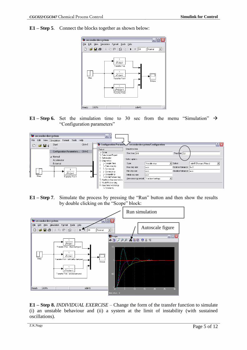
E1 – Step 5. Connect the blocks together as shown below:

E1 – Step 6. Set the simulation time to 30 sec from the menu “Simulation”

“Configuration parameters”

E1 – Step 7. Simulate the process by pressing the “Run” button and then show the results

by double clicking on the “Scope” block:

E1 – Step 8. INDIVIDUAL EXERCISE – Change the form of the transfer function to simulate

(i) an unstable behaviour and (ii) a system at the limit of instability (with sustained

oscillations).

Run simulation

Autoscale figure


Z.K.Nagy of 12

EXERCISE 2. Typical step response of First order Systems

E2 – Step 1. Start the Simulink environment by typing “simulink” to the matlab prompter.

E2 – Step 2. Open a new simulink mode from the File New Model

E2 – Step 3. Drag and drop the blocks below from the Simulink windows into the model

window (select “transfer function” from the “Continuous” group; “Step” from

“Sources”; “Scope” from “Sinks”, “Mux” from “Signal Routing”, etc.)

E2 – Step 4. Double click the blocks the set up different first order transfer functions.

Observe the effect of gain and time constant on the dynamic response of the

system.

E2 – Step 5. Identify which response belongs to which transfer function:

Transfer function 1 has response _____;



E2 – Step 6. INDIVIDUAL EXERCISE – Simulate various first, second and higher order

transfer functions:

(a) 1

0.1 1s; (b)

3 2

1

1s s s; (c)

3 2

1

2 2 1s s s; (d);

2

1

1s s

(e); 2

1

1

s

s s; (g)

2

1

1

s

s s; (e)

2

3 2

2 3 1

2 2 1

s s

s s s

(A)

(B)

(C)


Z.K.Nagy of 12

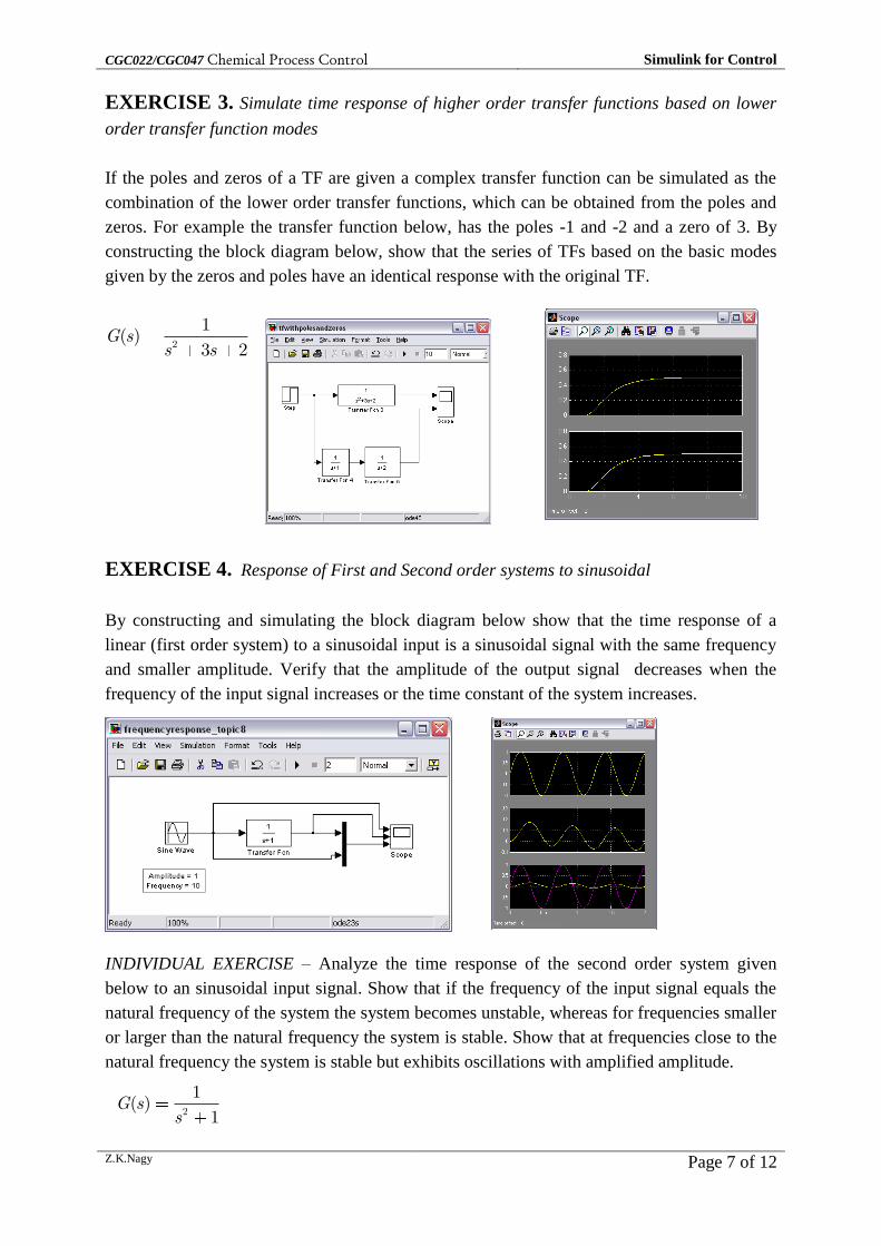
EXERCISE 3. Simulate time response of higher order transfer functions based on lower

order transfer function modes

If the poles and zeros of a TF are given a complex transfer function can be simulated as the

combination of the lower order transfer functions, which can be obtained from the poles and

zeros. For example the transfer function below, has the poles -1 and -2 and a zero of 3. By

constructing the block diagram below, show that the series of TFs based on the basic modes

given by the zeros and poles have an identical response with the original TF.

2

1( )

3 2G s

s s

EXERCISE 4. Response of First and Second order systems to sinusoidal

By constructing and simulating the block diagram below show that the time response of a

linear (first order system) to a sinusoidal input is a sinusoidal signal with the same frequency

and smaller amplitude. Verify that the amplitude of the output signal decreases when the

frequency of the input signal increases or the time constant of the system increases.

INDIVIDUAL EXERCISE – Analyze the time response of the second order system given

below to an sinusoidal input signal. Show that if the frequency of the input signal equals the

natural frequency of the system the system becomes unstable, whereas for frequencies smaller

or larger than the natural frequency the system is stable. Show that at frequencies close to the

natural frequency the system is stable but exhibits oscillations with amplified amplitude.

2

1( )

1G s

s


Z.K.Nagy of 12

EXERCISE 5. PID controller tuning using “practical” Ziegler-Nichols” technique.

Consider the following third order process (cascade of three reactors from the lecture Topic

13)

Tune a PID controller using a practical method and the Ziegler-Nichols tuning rules. The

method is often used in industry because it does not require to know the process transfer

function. It is based on the similar idea as the ZN method described in the lecture, with the

difference that the ultimate gain and ultimate period are determined experimentally, not

analytically.

E5 – Step1. Download the Simulink block diagram “model_3rdorder_PID.mdl” from the

LearnServer and save it in the current Matlab folder.

E5 – Step2. Set the controller to a P-only controller (by setting tau_I very large, e.g. tau_I =

100000; and tau_D = 0).

E5 – Step3. Start to give values to Kc until the closed loop system is at the verge of

instability (sustained oscillations are obtained)

E5 – Step 4. Determine from the figure the ultimate period (Tu). Use the zoom buttons in the

figure window and obtain the ultimate period (the

time interval for one entire oscillation).

E5 – Step 5. With the ultimate gain and period

determined at steps 3 and 5 compute the parameters

of a PID controller using the ZN tuning rules.

E5 – Step 6. Introduced the PID parameters in the

simulink PID controller and perform a simulations to

test the closed loop performance. Compare the values

of the ultimate gain and frequency and the tuning

parameters obtained with the “practical” approach

6( )

(2 1)(4 1)(6 1)pG s s s s

Ultimate period

Zoom buttons


Z.K.Nagy of 12

with those obtained using the analytical method (direct substitution) in the lecture (Topic 13).

EXERCISE 6. PID controller tuning using the Process Reaction Curve based Ziegler

Nichols approximate model approach.

Consider the same system as in EXERCISE 5. We will apply the approximate model based

ZN techniques for the PID controller tuning. According to this approach (see lecture on Topic

13) first an approximate FOPTD representation of the process is identified based on the

process reaction curve and then the PID controller parameters are obtained using the

appropriate ZN tuning rules.

E6 – Step 1. Download the Simulink program “model_3rdorder_FOPTD.mdl” and save it in

the current Matlab folder.

E6 – Step 2. Open the model and change the gain, time constant and time-delays of the

approximate model to obtain a response which is as close as possible to the original process

response. After each change simulate the two systems by pressing the run Button.

E6 – Step 3. Use the effective time constant, effective gain and effective time delay obtained in

Step 2 (which provides the best approximations of the original third order system) and

calculate the PID controller parameters using the ZN tuning rules (lecture – Topic 13, slide

25)

E6 – Step 4. Use the calculated tuning parameters in the block diagram from Exercise 5 to

simulate the closed loop response. Compare the tuning parameters obtained in this case with

those resulted in Exercise 5. Compare the closed loop performance in the two cases.


Z.K.Nagy of 12

EXERCISE 7. PID controller tuning using the IMC tuning rule.

E7 – Step 1. Download the file model “Ex_IMC.mdl” and save in the current Matlab folder.

The block diagram simulates the FOPTD system given in Example 2 from the lecture notes

(Topic 14 part 2, slide 19):

In the block diagram the closed loop system is simulated twice for comparison.

E7 – Step 2. Tune the first PID according to the ZN approach based on approximate model.

This is straightforward since the transfer function is already in the FOPTD form.

E7 – Step 3. Tune the second PID using the IMC tuning rules derived in the lecture note

(Topic 14 part 2, slide 11):

1 1( ) (1

12

9.59

9.5

5( 1.5))

.5cG s s

s

which gives I = 9.5 and D= 1.26 and a gain that

depends on . Calculate the gain for different values (e.g. 1, 2, and 5), run the simulation

for each set if tuning parameters and compare the closed loop performance with the ZN

tuning.

35( )

8 1

s

p

eG s

s


Z.K.Nagy of 12

EXERCISE 8. Cascade control

E8 – Step 1. Download the simulink file “model3rdorder_PID_nocascade”. This represents

the model of jacketed chemical reactor where the jacket input temperature – jacket

temperature dynamics is model by a first order system whereas the jacket temperature to

reactor temperature dynamics by a second order system, leading to a third order system

overall, similar as in example as in Exercise 5.

E8– Step 2. Simulate the system using the simple control loop, which controls the reactor

temperature via the jacket inlet temperature directly. Tune this controller using any method.

E8 – Step 3. Construct and simulate a typical cascade control of the reactor temperature, and

compare the control performance compared to step 2. Use in the first instance the same gain

and integral time for both the slave and master controllers. IMPORTANT: Do not use any

derivative action for the slave controller.


Z.K.Nagy of 12

Individual exercises for self study

1. Download the simulink diagram that simulates the input output behaviour of a chemical

process with unknown model (“blackbox_model.mdl”). Apply your Chemical Process

Control knowledge and design a controller for the process. Prepare the Simulink diagram

and simulate the closed loop response of the resulted system.

Hint. You may use any (or all) of the PID controller tuning approaches learned in the

module (e.g. you can identify a FOPDT model based on the process reaction curve, or you

can use the practical ZN tuning via the experimental determination of the ultimate gain and

ultimate period.

2. Look up in the textbook the guidelines for tuning the controllers in the cascade control

architecture and follow these guidelines to tune the controllers from Exercise 8.

3. Write a Matlab function and use it or quantitative comparison of the control performances

in the exercises above. You can compute for example the sum-of-squares error criteria.

Simulink4Controlnew2008_1page

Documents

Transcript of Simulink4Controlnew2008_1page