UNIVERSITY OF THE WEST INDIES

ST. AUGUSTINE FACULTY OF ENGINEERING

DEPARTMENT OF CHEMICAL ENGINEERING

CHNG 2003 – Computer Aided Engineering 2010-2011

SIMULINK Tutorial

Objective: The aim of this lab is to translate each model equation into a sequence of blocks, and to connect them in the appropriate way to form a “system.” The variables in the equations become signals that vary with time. Most Simulink blocks perform mathematical operations on input signals to generate one or more output signals.

Example 1

Modeling an algebraic equation

For example, consider the linear equation, y = mx + b, where m and b are constants. Suppose

m=2, and b=3. Let x be an independent function of time. Given x, you could easily calculate the

dependent variable, y, without resorting to a simulation, but it’s a good starting point to illustrate

Simulink concepts.

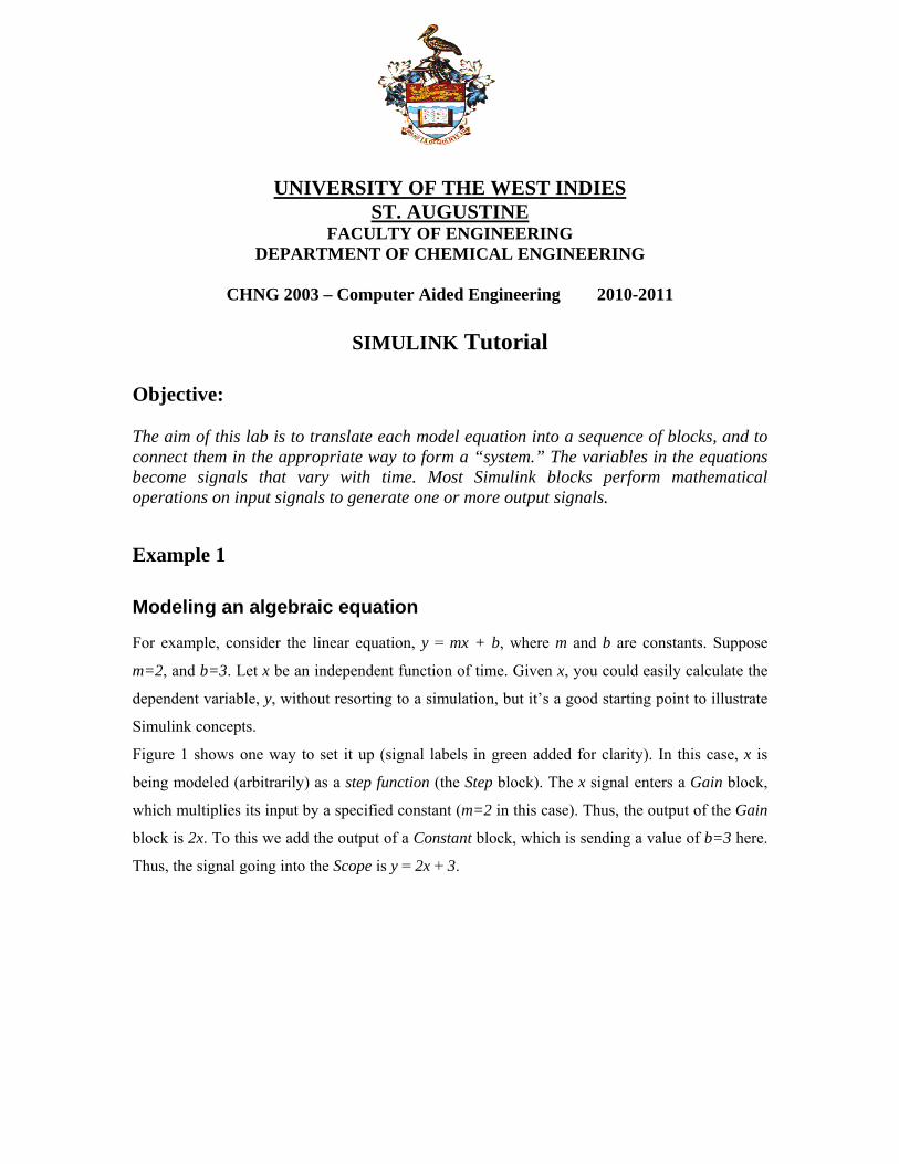
Figure 1 shows one way to set it up (signal labels in green added for clarity). In this case, x is

being modeled (arbitrarily) as a step function (the Step block). The x signal enters a Gain block,

which multiplies its input by a specified constant (m=2 in this case). Thus, the output of the Gain

block is 2x. To this we add the output of a Constant block, which is sending a value of b=3 here.

Thus, the signal going into the Scope is y = 2x + 3.

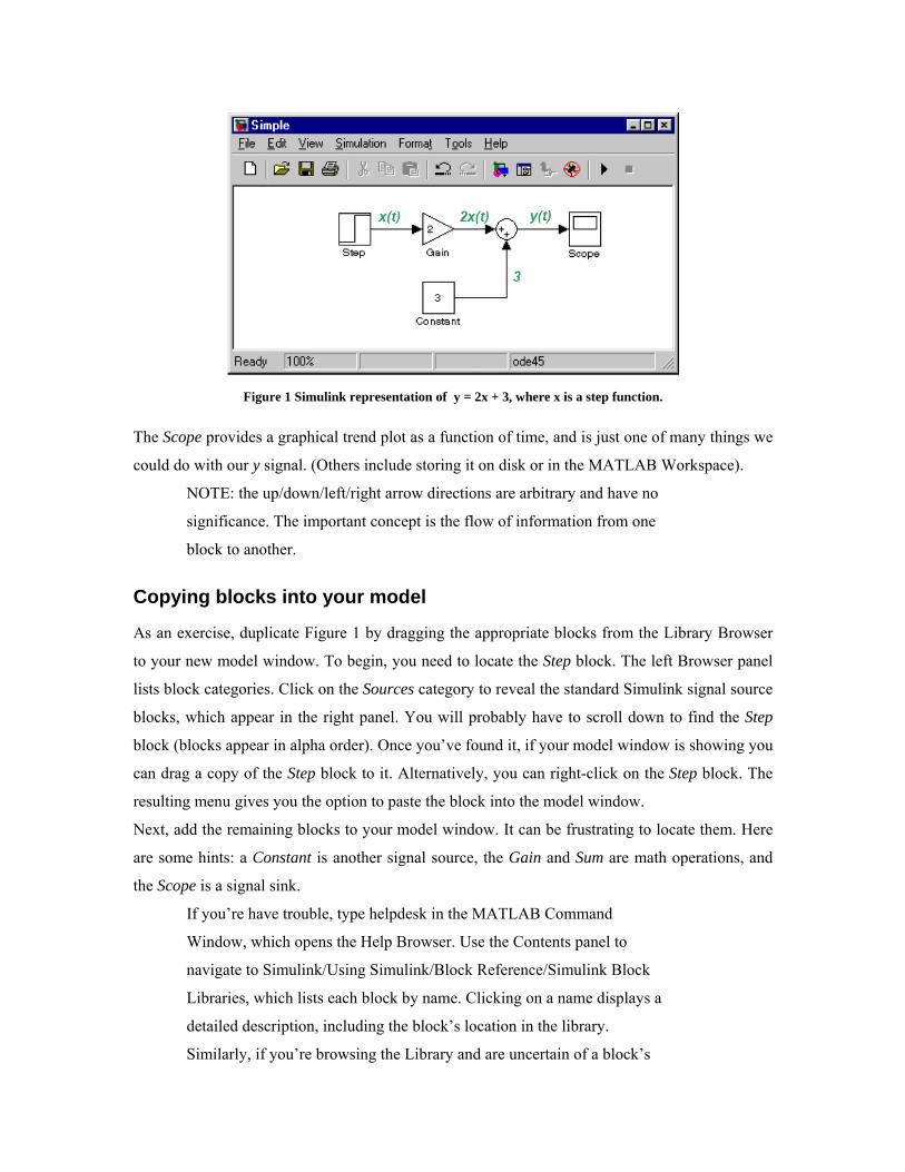
Figure 1 Simulink representation of y = 2x + 3, where x is a step function.

The Scope provides a graphical trend plot as a function of time, and is just one of many things we

could do with our y signal. (Others include storing it on disk or in the MATLAB Workspace).

NOTE: the up/down/left/right arrow directions are arbitrary and have no

significance. The important concept is the flow of information from one

block to another.

Copying blocks into your model

As an exercise, duplicate Figure 1 by dragging the appropriate blocks from the Library Browser

to your new model window. To begin, you need to locate the Step block. The left Browser panel

lists block categories. Click on the Sources category to reveal the standard Simulink signal source

blocks, which appear in the right panel. You will probably have to scroll down to find the Step

block (blocks appear in alpha order). Once you’ve found it, if your model window is showing you

can drag a copy of the Step block to it. Alternatively, you can right-click on the Step block. The

resulting menu gives you the option to paste the block into the model window.

Next, add the remaining blocks to your model window. It can be frustrating to locate them. Here

are some hints: a Constant is another signal source, the Gain and Sum are math operations, and

the Scope is a signal sink.

If you’re have trouble, type helpdesk in the MATLAB Command

Window, which opens the Help Browser. Use the Contents panel to

navigate to Simulink/Using Simulink/Block Reference/Simulink Block

Libraries, which lists each block by name. Clicking on a name displays a

detailed description, including the block’s location in the library.

Similarly, if you’re browsing the Library and are uncertain of a block’s

purpose, right-click on it and select help to see the detailed description.

Also, the Library Browser’s upper panel provides a brief description of

the selected block.

Entering block parameters

You should now have the five required blocks in your model window, arranged as shown

in Figure 2. The Gain and Constant values are incorrect, however (the defaults are 1). To

fix these, double-click on each, and enter the desired value in the parameter box.

Figure 2 Blocks copied from the standard Simulink library

Connecting blocks

The small > symbol on the right side of the Step block marks its “outport.” Note the “inport” on

the Gain block’s left side. Click and drag from the Step’s outport to the Gain’s inport to connect

them. The resulting signal line must have a solid, filled-in arrowhead, as in Figure 1. If not, the

blocks aren’t connected; try again. Similarly, connect the rest of the blocks until you obtain the

result shown earlier in Figure 1. Note the way Simulink automatically makes a neat right-angle

connection when you connect the Constant to the Sum.

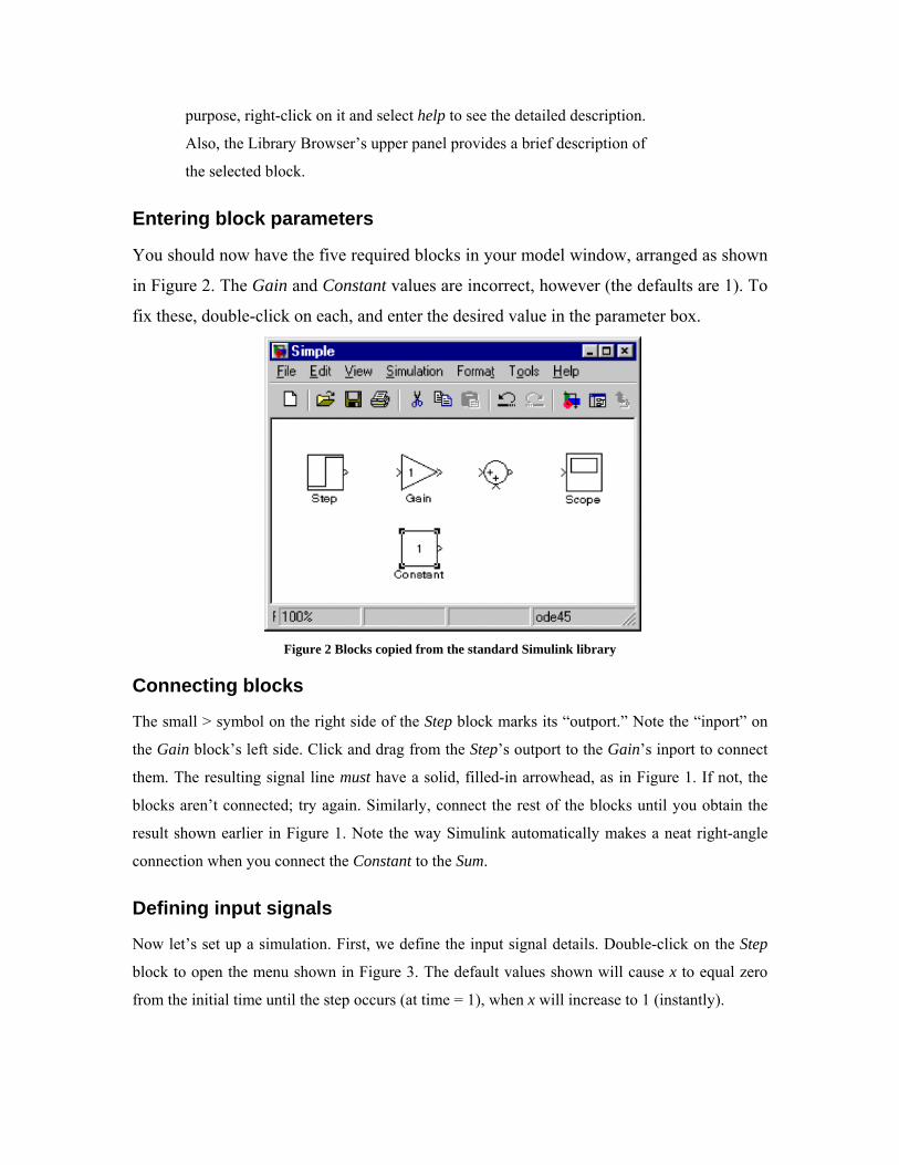
Defining input signals

Now let’s set up a simulation. First, we define the input signal details. Double-click on the Step

block to open the menu shown in Figure 3. The default values shown will cause x to equal zero

from the initial time until the step occurs (at time = 1), when x will increase to 1 (instantly).

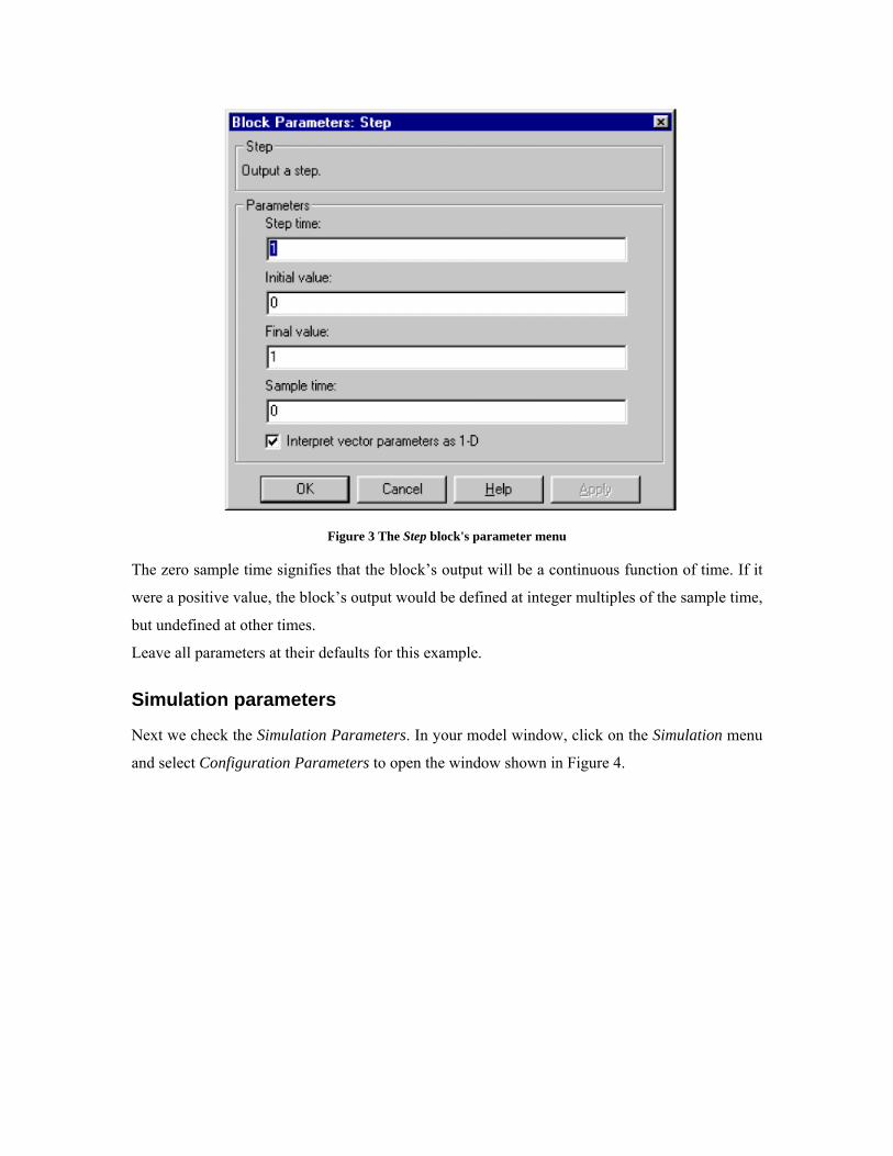
Figure 3 The Step block's parameter menu

The zero sample time signifies that the block’s output will be a continuous function of time. If it

were a positive value, the block’s output would be defined at integer multiples of the sample time,

but undefined at other times.

Leave all parameters at their defaults for this example.

Simulation parameters

Next we check the Simulation Parameters. In your model window, click on the Simulation menu

and select Configuration Parameters to open the window shown in Figure 4.

Figure 4 Simulation parameters menu, Solver panel

The left side allows you to navigate to various configuration panels. The Solver panel (selected in

Figure 4) allows you to specify the time at which the simulation starts and stops (which depends

on the time scale of your problem). Note also the Solver options. The default solver, ode45, is a

variable-step-size, 4th

-order Runge Kutta algorithm, which is a good all-around choice, but is poor

for stiff problems, and there are situations where a fixed-step-size algorithm would be better. See

the Simulink Help for details. We’ll use ode45 in this simple example.

You can usually use the defaults for the remaining parameters on this panel, but if you suspect

that your results are inaccurate, try decreasing the relative tolerance by an order of magnitude or

two. If the results change significantly, decrease it even further. Direct control of the step size can

also be useful, as we’ll see later.

The Data Import/Export panel controls communication between MATLAB and Simulink. You

might find this valuable in some cases, but we’ll use the defaults for this and all other panels.

Close the configuration window. As the final preparation for the simulation, double-click on the

Scope to open the graphical display.

Figure 5 Ready to start the simulation

Running the simulation

Now click the Start Button (see Figure 5). The simulation begins (the Start button changes to a

Pause icon, and the Stop button to its right becomes active). The elapsed time appears in the box

just to the left of the simulation option (bottom of model window) and the y signal trace appears

on the scope. (NOTE: this simulation is trivial and runs so rapidly that you probably won’t be

able to see things changing.) On a computer with sound you should hear a beep when the

simulation ends.

Figure 6 Scope display of the y signal

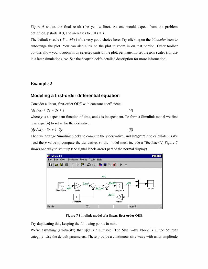
Figure 6 shows the final result (the yellow line). As one would expect from the problem

definition, y starts at 3, and increases to 5 at t = 1.

The default y scale (-5 to +5) isn’t a very good choice here. Try clicking on the binocular icon to

auto-range the plot. You can also click on the plot to zoom in on that portion. Other toolbar

buttons allow you to zoom in on selected parts of the plot, permanently set the axis scales (for use

in a later simulation), etc. See the Scope block’s detailed description for more information.

Example 2

Modeling a first-order differential equation

Consider a linear, first-order ODE with constant coefficients

(dy / dt) + 2y = 3x + 1 (4)

where y is a dependent function of time, and x is independent. To form a Simulink model we first

rearrange (4) to solve for the derivative,

(dy / dt) = 3x + 1- 2y (5)

Then we arrange Simulink blocks to compute the y derivative, and integrate it to calculate y. (We

need the y value to compute the derivative, so the model must include a “feedback”.) Figure 7

shows one way to set it up (the signal labels aren’t part of the normal display).

Figure 7 Simulink model of a linear, first-order ODE

Try duplicating this, keeping the following points in mind:

We’re assuming (arbitrarily) that x(t) is a sinusoid. The Sine Wave block is in the Sources

category. Use the default parameters. These provide a continuous sine wave with unity amplitude

and a frequency of 1 radian per time unit (the documentation claims that the time unit is seconds,

but that isn’t true in general as explained previously). Thus, the sine wave’s period will be 2π

time units.

Drag a Gain block in from the Library Browser, then use control-click and drag to make a copy.

Simulink requires all the block names in a system to be unique. and it automatically assigns a new

name to copied blocks (e.g., Gain 1). Then right-click on the copy and select Format/Flip Block

to reverse its direction (you can also rotate, etc.).

Duplicate the Sum block. By default, Simulink hides its name, but each is unique. (You can right-

click and use the format menu to show the name if you wish.) One of the Sum blocks must do a

subtraction. To accomplish this, double-click on the block and edit the sign symbols in the block

parameter box. Try different combinations of the signs (and the vertical bar), clicking apply each

time to see the effect (or read the block help). You can add a third input by including a third sign

symbol. (If you have more than three inputs, use the rectangular block shape instead.)

The Integrator block is from the Continuous category. The 1/s icon derives from Laplace

transforms. Its key parameter is the initial condition, which sets the value of its output when the

simulation begins (i.e., y(0) in our case). Use the default (zero).

The black vertical bar just to the left of the scope is a Mux block (from Signals & Systems). It

combines the scalar x(t) and y(t) signals into a vector signal so we can plot x(t) and y(t) on the

same graph window. Another way would be to define two scopes, one connected to each scalar

signal, which would be better if the x and y magnitudes were very different. You can also define

multiple axes for a single scope block, in which case the block will have multiple inports and its

display window will be split to show each axis.

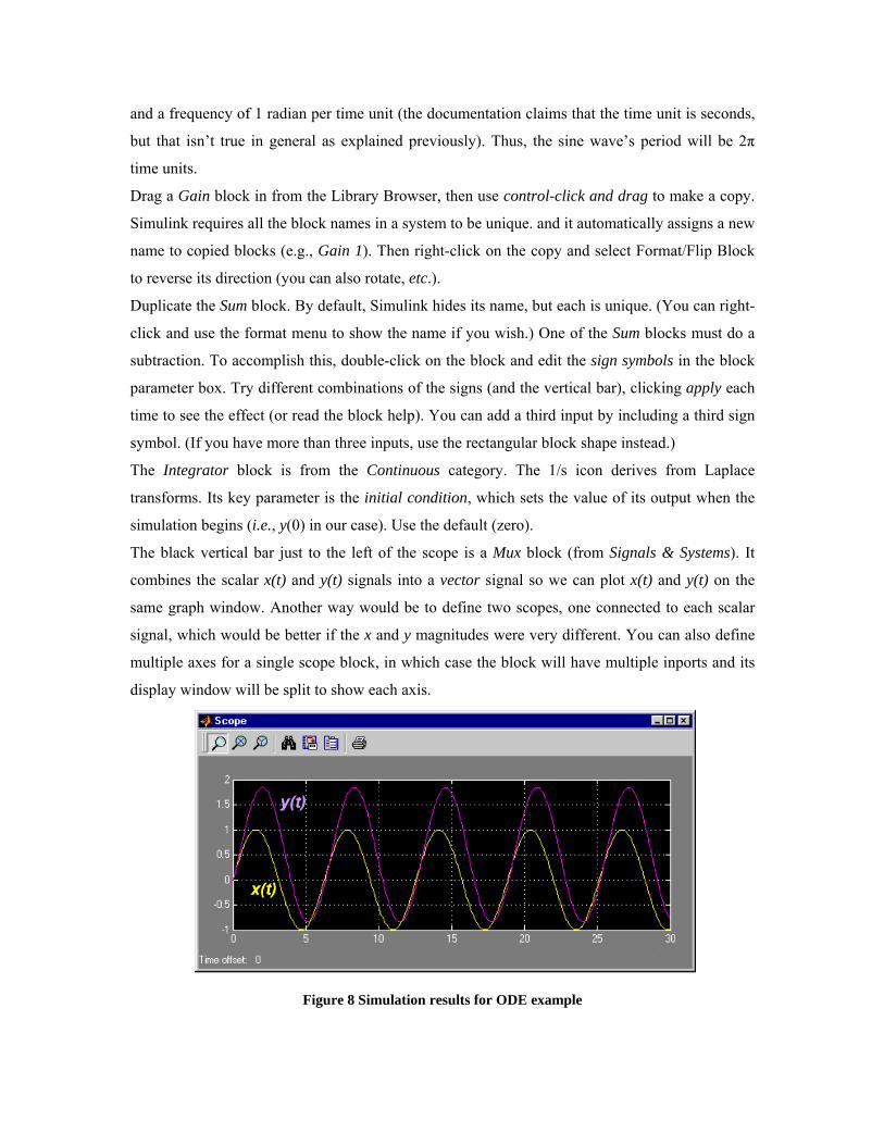
Figure 8 Simulation results for ODE example

The small black dots on two of the signal lines are solder junctions (another EE influence). All

lines entering/leaving a solder junction carry the same signal. To make a solder junction, move

the cursor to the desired location, and then control-click-and-drag to start drawing the new signal

line. After you’ve made a solder joint you can move it around by clicking-and-dragging. You can

also move signal line sections and blocks. It’s possible for signal lines to cross without forming a

solder junction (try it). In that case, the signals are independent.

Set the stop time to 30. The most convenient way is to edit the value at the top of the model

window. To make the plots look better, set the maximum step size to 0.1. Next, run the simulation

Figure 8 shows the results (with superimposed x(t) and y(t) signal labels for clarity). Use the

binoculars icon to zoom in on the curves. The steady sinusoidal input, x(t), eventually causes a

sinusoidal output having the same frequency but a different phase. We will study such frequency

responses in more detail later.

Using subsystems

Modeling a single algebraic or differential equation is fairly easy, but what about multi-equation

models? It’s really no different. You define each equation and its variables (signals), then

combine equations by connecting their common signals.

One problem is that the diagram can become complicated, making it hard to understand the

model. You can reduce the apparent complexity by defining subsystems, each of which models

part of the complete system. This is conceptually similar to the use of functions and subprograms

in computer languages.

Example 3 For example, consider combining (5) with another differential equation:

( dz / dt ) = 2x – y – 3z

Adding this to our previous model would be easy, and the diagram would still be fairly clear, but

we will use subsystems to illustrate the concept.

Start with a new model window. Drag in a SubSystem block (from the Ports and Subsystems

category). Edit the block name, changing it to “Equation 5”. Next make a copy, naming it

“Equation 6.” Your model window should now resemble Figure 9 (name the model TwoODEs).

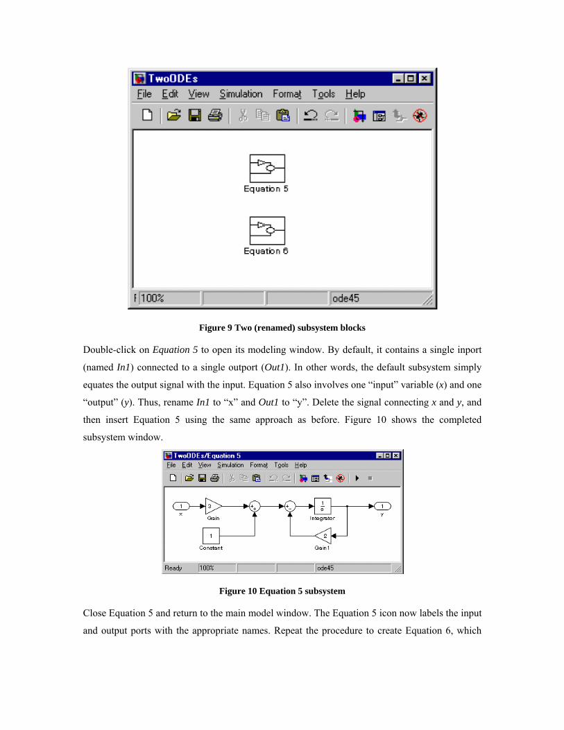
Figure 9 Two (renamed) subsystem blocks

Double-click on Equation 5 to open its modeling window. By default, it contains a single inport

(named In1) connected to a single outport (Out1). In other words, the default subsystem simply

equates the output signal with the input. Equation 5 also involves one “input” variable (x) and one

“output” (y). Thus, rename In1 to “x” and Out1 to “y”. Delete the signal connecting x and y, and

then insert Equation 5 using the same approach as before. Figure 10 shows the completed

subsystem window.

Figure 10 Equation 5 subsystem

Close Equation 5 and return to the main model window. The Equation 5 icon now labels the input

and output ports with the appropriate names. Repeat the procedure to create Equation 6, which

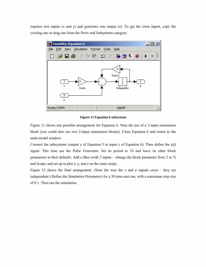
requires two inputs (x and y) and generates one output (z). To get the extra inport, copy the

existing one or drag one from the Ports and Subsystems category.

Figure 11 Equation 6 subsystem

Figure 11 shows one possible arrangement for Equation 6. Note the use of a 3-input summation

block (you could also use two 2-input summation blocks). Close Equation 6 and return to the

main model window.

Connect the subsystems (output y of Equation 5 to input y of Equation 6). Then define the x(t)

signal. This time use the Pulse Generator. Set its period to 10 and leave its other block

parameters at their defaults. Add a Mux (with 3 inputs – change the block parameter from 2 to 3)

and Scope, and set up to plot x, y, and z on the same scope.

Figure 12 shows the final arrangement. (Note the way the x and y signals cross – they are

independent.) Define the Simulation Parameters for a 30 time-unit run, with a maximum step size

of 0.1. Then run the simulation

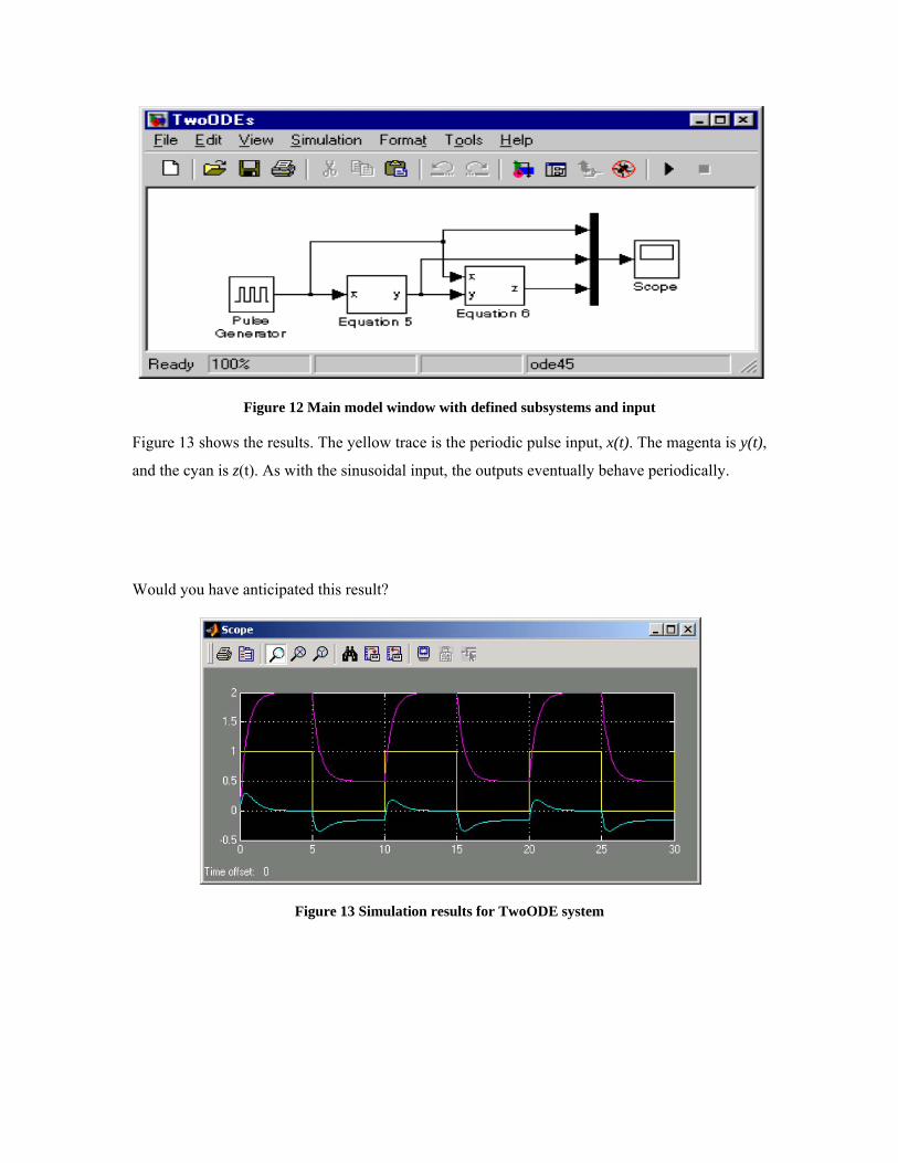
Figure 12 Main model window with defined subsystems and input

Figure 13 shows the results. The yellow trace is the periodic pulse input, x(t). The magenta is y(t),

and the cyan is z(t). As with the sinusoidal input, the outputs eventually behave periodically.

Would you have anticipated this result?

Figure 13 Simulation results for TwoODE system