Simulation Study of Hemispheric Phase-Asymmetry in the Solar Cycle

D. Shukuya Institute for Space-Earth Environmental Research, Nagoya University

Furo-cho Chikusa-ku, Nagoya, Aichi 4648601, Japan.

K. Kusano Institute for Space-Earth Environmental Research, Nagoya University

Furo-cho, Chikusa-ku, Nagoya, Aichi 4648601, Japan. kusano@nagoya-u.jp

Abstract Observations of the sun suggest that solar activities systematically create north-south hemispheric asymmetries. For instance, the hemisphere in which the sunspot activity is more active tends to switch after the early half of each solar cycle. Svalgaard & Kamide (2013) recently pointed out that the time gaps of polar field reversal between the north and south hemispheres are simply consequences of the asymmetry of sunspot activity. However, the mechanism underlying the asymmetric feature in solar cycle activities is not yet well understood. In this paper, in order to explain the cause of the asymmetry from the theoretical point of view, we investigate the relationship between the dipole- and quadrupole-type components of the magnetic field in the solar cycle using the mean-field theory based on the flux transport dynamo model. As a result, we found that there are two different attractors of the solar cycle, in which either the north or the south polar field is first reversed, and that the flux transport dynamo model well explains the phase-asymmetry of sunspot activity and the polar field reversal without any ad hoc source of asymmetry. Key words: dynamo – methods: numerical – Sun: evolution – Sun: interior – Sun: magnetic fields

1. INTRODUCTION Various kinds of hemispheric asymmetry in the northern and southern hemispheres have

been observed in solar magnetic activities, e.g., sunspot numbers, sunspot area, flares, prominences, faculae, coronal brightness, and the time of polar magnetic field reversal (see e.g., Maunder 1890, 1904, Waldmeier 1971, Roy 1977, and Babcock 1959). According to Waldmeier (1971), for instance, the phase of sunspot cycle 19 was shifted between the northern and the southern hemispheres, such that the sunspot cycle in the southern hemisphere reached the maximum approximately one year earlier than that in the northern hemisphere. In addition, it was reported that the polar magnetic field reversal at one pole is delayed for one or two years compared with the other pole in every solar cycle (Babcock 1959, Li 2009, Murakozy & Ludmany 2012, Shiota et al. 2012, and Svalgaard & Kamide 2013). Based on the observation of sunspot groups during the last 12 solar cycles, Li (2009) and Murakozy & Ludmany (2012) pointed out that the leading hemisphere, in which the magnetic activities are more active than the other in the early half-phase of each cycle, may switch after approximately an eight-sunspot-cycle period. These observational results imply that certain systematic processes in addition to a stochastic process govern the asymmetries of the solar cycle. However, the mechanisms underlying this have not yet been clearly explained. The solar magnetic field is considered to be sustained by the dynamo action in the interior of the sun (Parker 1955). After the helioseismology revealed the averaged distribution of the large-scale internal velocity field, i.e., the meridional circulation and the differential rotation (Thompson et al. 2003), the flux transport dynamo model was proposed (Choudhuri et al. 1995, Dikpati & Charbonneau 1999, Nandy & Choudhuri 2002, and Chatterjee, Nandy, & Choudhuri (hereafter CNC) 2004) as a promising model to explain certain features of solar magnetic activities, such as the 11-year cycle, the butterfly diagram, the poleward migration of surface field, and polarity reversals of the polar field. Since the computation of the flux transport model is not numerically demanding, numerical simulations based on this model are widely used as a tool to study the variation in the solar cycle.

In previous studies, several numerical models ware developed to explain the asymmetric features of the solar cycle (e.g., DeRosa et al. 2012, Brun et al. 2013, Belucz et al. 2013, Belucz & Dikpati 2013, Olemskoy & Kitchatinov 2013, and Shetye et al. 2015). DeRosa et al. (2012) and Brun et al. (2013) showed that a certain degree of asymmetric modulation to the source of the poloidal field or the meridional circulation causes the interaction between the primary family and the secondary family of the magnetic field and produces the time gaps of the polar magnetic field reversals between the north and the south poles. The primary family is a dipole-type part, which is the spherical harmonic functions of

the surface magnetic field 𝐵𝐵𝑙𝑙0 with 𝑙𝑙 = 1, 3, 5, 7,⋯, and the secondary family is a quadrupole-type part, which is 𝐵𝐵𝑙𝑙0 with 𝑙𝑙 = 2, 4, 6, 8,⋯. Belucz et al. (2013) showed that the dynamo operates mostly independently in the northern and the southern hemispheres by studying the features of the dynamo operating with the source terms of poloidal field of different amplitudes between the different hemispheres. Belucz & Dikpati (2013) showed that when the amplitude or pattern of the meridional circulation changed only for the southern hemisphere, the dynamo period, the shape of the butterfly diagram, the strength of the polar and toroidal fields, and the phase relations between the polar and toroidal fields changed almost exclusively for the southern hemisphere. Olemskoy & Kitchatinov (2013) introduced the fluctuating poloidal field source term into the mean-field dynamo model using a smoothly varying random function of time and latitude. As a consequence, it was shown that the fluctuations violate hemispheric symmetry of the dynamo field. When the deviations from dipole parity are large, the model shows weak magnetic cycles, in which the large asymmetry of magnetic activity appears like the sunspot in grand minima. Passos et al. (2013) also studied the origin of hemispheric asymmetry and cycle amplitude modulation by introducing independent stochastic fluctuations in the two hemispheres using the mean-field dynamo model, and they demonstrated many types of hemispheric asymmetries, including grand minima and failed grand minima where only one hemisphere enters a quiescent state. Shetye et al. (2015) discussed the contribution of active-region fluxes and their hemispheric asymmetries. They introduced the asymmetric active-region inflow effect to the meridional circulation and found that the inflow can affect peak amplitude of the solar cycle. Observations by local helioseismology indicate that the meridional motions of active regions generate inflows, which are meridional converging flows into active regions at the solar surface from lower and higher latitudes (Gizon & Birch 2005).

These previous studies indicate that the symmetric properties of the dynamo are obviously affected by the asymmetric flow or magnetic field, which is ad hoc imposed in the dynamo equation. However, the cause of this asymmetry is still open to question. The objective of this paper is to elucidate whether the asymmetric properties in the solar dynamo are capable of being spontaneously created even though the flow is symmetric with respect to the equator. When the flow is symmetric the dynamo equation is known to have two different types of solutions, i.e., the so-called dipole-type and quadrupole-type families (Jennings & Weiss 1991 and Nishikawa & Kusano 2008). Since these fields have different parities of hemispheric symmetry, their mixing might cause the asymmetries. Our study was originally motivated by this property of the dynamo equation. Since dynamo is a nonlinear process in which flow and magnetic field mutually interact, it is not easy to elucidate what is the fundamental cause of the asymmetric property. However, if some asymmetry is created

even though any external conditions (e.g., flow, source terms, and diffusion) are symmetric, we could conclude that the asymmetric property of the dynamo is inherent in the dynamo equation. To achieve this, we developed a standard flux transport dynamo code based on the SURYA code (CNC 2004) and carefully analyzed the asymmetric features of the solar magnetic activities. Finally, we will propose that the solar cycle may spontaneously create the hemispheric asymmetry.

2. SIMULATION MODEL 2.1. Basic Equations

We solve the axisymmetric mean-field kinematic dynamo equations on a meridional plane of a rotating spherical shell (𝑅𝑅b = 0.55𝑅𝑅⨀ ≤ 𝑟𝑟 ≤ 𝑅𝑅⨀, 0 ≤ 𝜃𝜃 ≤ 𝜋𝜋, where 𝑅𝑅𝑏𝑏, 𝑅𝑅⨀, 𝑟𝑟, and

𝜃𝜃 denote the radius of the bottom boundary, the solar radius, the radial coordinate, and the colatitude, respectively). The shell is rotating with an angular velocity 𝜴𝜴 = 𝛺𝛺𝒆𝒆𝑧𝑧, where 𝒆𝒆𝑧𝑧 is a unit vector along the rotation axis. Hereafter, 𝒆𝒆𝑖𝑖 denotes a unit vector along the 𝑖𝑖 coordinate. Under the axisymmetric approximation, the azimuthally averaged magnetic field

𝑩𝑩(𝑟𝑟, 𝜃𝜃, 𝑡𝑡) and velocity field 𝑽𝑽(𝑟𝑟,𝜃𝜃) can be decomposed into the poloidal and toroidal components, respectively:

𝑩𝑩(𝑟𝑟, 𝜃𝜃, 𝑡𝑡) = 𝑩𝑩𝒑𝒑(𝑟𝑟, 𝜃𝜃, 𝑡𝑡) + 𝐵𝐵(𝑟𝑟, 𝜃𝜃, 𝑡𝑡)𝒆𝒆𝜙𝜙= 𝛁𝛁×�𝐴𝐴(𝑟𝑟, 𝜃𝜃, 𝑡𝑡)𝒆𝒆𝜙𝜙�+ 𝐵𝐵(𝑟𝑟,𝜃𝜃, 𝑡𝑡)𝒆𝒆𝜙𝜙,

(1)

𝑽𝑽(𝑟𝑟,𝜃𝜃) = 𝒗𝒗𝒑𝒑(𝑟𝑟, 𝜃𝜃) + 𝑟𝑟 sin 𝜃𝜃 𝛺𝛺(𝑟𝑟, 𝜃𝜃)𝒆𝒆𝜙𝜙= 𝑣𝑣𝑟𝑟𝒆𝒆𝑟𝑟 + 𝑣𝑣𝜃𝜃𝒆𝒆𝜃𝜃 + 𝑟𝑟 sin𝜃𝜃 𝛺𝛺(𝑟𝑟,𝜃𝜃)𝒆𝒆𝜙𝜙,

(2)

in which the poloidal magnetic field 𝑩𝑩𝒑𝒑(𝑟𝑟, 𝜃𝜃, 𝑡𝑡) is described by the toroidal (𝜙𝜙) component of

the vector potential 𝐴𝐴(𝑟𝑟, 𝜃𝜃, 𝑡𝑡) as 𝑩𝑩𝒑𝒑(𝑟𝑟, 𝜃𝜃, 𝑡𝑡) = ∇×�𝐴𝐴(𝑟𝑟, 𝜃𝜃, 𝑡𝑡)𝒆𝒆𝜙𝜙� . The vectors, 𝐵𝐵(𝑟𝑟,𝜃𝜃, 𝑡𝑡)𝒆𝒆𝜙𝜙 and 𝒗𝒗𝒑𝒑(𝑟𝑟,𝜃𝜃), are the toroidal component of magnetic field and the poloidal component of

velocity field (meridional flow), respectively. Using Equations (1) and (2), the basic equations for the so-called 𝛼𝛼𝛼𝛼 dynamo are

𝜕𝜕𝐵𝐵𝜕𝜕𝑡𝑡

+1𝑟𝑟 �

𝜕𝜕𝜕𝜕𝑟𝑟

(𝑟𝑟𝑣𝑣𝑟𝑟𝐵𝐵) +𝜕𝜕𝜕𝜕𝜃𝜃

(𝑣𝑣𝜃𝜃𝐵𝐵)�

= 𝜂𝜂𝑡𝑡 �∇2 −1𝑠𝑠2�𝐵𝐵 +

1𝑟𝑟𝑑𝑑𝜂𝜂𝑡𝑡𝑑𝑑𝑟𝑟

𝜕𝜕𝜕𝜕𝑟𝑟

(𝑟𝑟𝐵𝐵) + 𝑠𝑠(𝑩𝑩𝑃𝑃 ∙ 𝛁𝛁)𝛺𝛺,

(3)

𝜕𝜕𝐴𝐴𝜕𝜕𝑡𝑡

+1𝑠𝑠

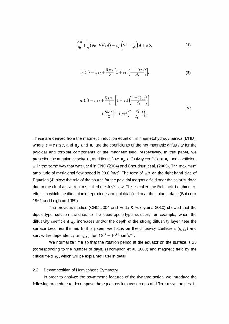
(𝒗𝒗𝑃𝑃 ∙ 𝛁𝛁)(𝑠𝑠𝐴𝐴) = 𝜂𝜂𝑝𝑝 �∇2 −1𝑠𝑠2�𝐴𝐴 + 𝛼𝛼𝐵𝐵, (4)

𝜂𝜂𝑝𝑝(𝑟𝑟) = 𝜂𝜂𝑅𝑅𝑅𝑅 +

𝜂𝜂𝑆𝑆𝑆𝑆𝑅𝑅2 �1 + erf �

𝑟𝑟 − 𝑟𝑟𝐵𝐵𝑆𝑆𝑅𝑅𝑑𝑑𝑡𝑡

��, (5)

𝜂𝜂𝑡𝑡(𝑟𝑟) = 𝜂𝜂𝑅𝑅𝑅𝑅 +

𝜂𝜂𝑆𝑆𝑆𝑆𝑅𝑅12

�1 + erf�𝑟𝑟 − 𝑟𝑟𝐵𝐵𝑆𝑆𝑅𝑅′

𝑑𝑑𝑡𝑡��

+𝜂𝜂𝑆𝑆𝑆𝑆𝑅𝑅

2 �1 + erf �𝑟𝑟 − 𝑟𝑟𝑇𝑇𝑆𝑆𝑅𝑅𝑑𝑑𝑡𝑡

��. (6)

These are derived from the magnetic induction equation in magnetohydrodynamics (MHD), where 𝑠𝑠 = 𝑟𝑟 sin 𝜃𝜃, and 𝜂𝜂𝑝𝑝 and 𝜂𝜂𝑡𝑡 are the coefficients of the net magnetic diffusivity for the

poloidal and toroidal components of the magnetic field, respectively. In this paper, we prescribe the angular velocity 𝛺𝛺, meridional flow 𝒗𝒗𝑝𝑝, diffusivity coefficient 𝜂𝜂𝑡𝑡, and coefficient

𝛼𝛼 in the same way that was used in CNC (2004) and Choudhuri et al. (2005). The maximum amplitude of meridional flow speed is 29.0 [m/s]. The term of 𝛼𝛼𝐵𝐵 on the right-hand side of Equation (4) plays the role of the source for the poloidal magnetic field near the solar surface

due to the tilt of active regions called the Joy’s law. This is called the Babcock–Leighton 𝛼𝛼-effect, in which the tilted bipole reproduces the poloidal field near the solar surface (Babcock 1961 and Leighton 1969). The previous studies (CNC 2004 and Hotta & Yokoyama 2010) showed that the dipole-type solution switches to the quadrupole-type solution, for example, when the diffusivity coefficient 𝜂𝜂𝑝𝑝 increases and/or the depth of the strong diffusivity layer near the

surface becomes thinner. In this paper, we focus on the diffusivity coefficient (𝜂𝜂𝑆𝑆𝑆𝑆𝑅𝑅 ) and

survey the dependency on 𝜂𝜂𝑆𝑆𝑆𝑆𝑅𝑅 for 1011 − 1013 cm2s−1. We normalize time so that the rotation period at the equator on the surface is 25 (corresponding to the number of days) (Thompson et al. 2003) and magnetic field by the

critical field 𝐵𝐵𝑐𝑐, which will be explained later in detail. 2.2. Decomposition of Hemispheric Symmetry

In order to analyze the asymmetric features of the dynamo action, we introduce the following procedure to decompose the equations into two groups of different symmetries. In

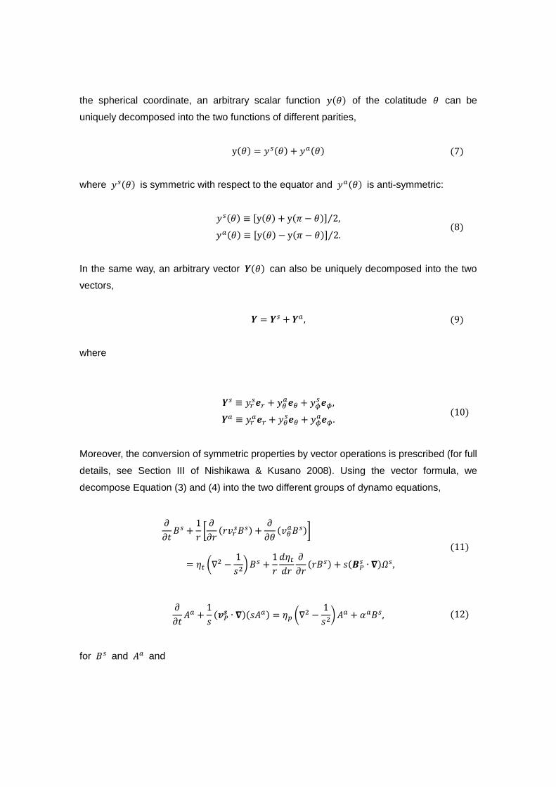
the spherical coordinate, an arbitrary scalar function 𝑦𝑦(𝜃𝜃) of the colatitude 𝜃𝜃 can be uniquely decomposed into the two functions of different parities,

y(𝜃𝜃) = 𝑦𝑦𝑠𝑠(𝜃𝜃) + 𝑦𝑦𝑎𝑎(𝜃𝜃) (7)

where 𝑦𝑦𝑠𝑠(𝜃𝜃) is symmetric with respect to the equator and 𝑦𝑦𝑎𝑎(𝜃𝜃) is anti-symmetric:

𝑦𝑦𝑠𝑠(𝜃𝜃) ≡ [y(𝜃𝜃) + y(𝜋𝜋 − 𝜃𝜃)] 2⁄ , 𝑦𝑦𝑎𝑎(𝜃𝜃) ≡ [y(𝜃𝜃)− y(𝜋𝜋 − 𝜃𝜃)] 2⁄ .

(8)

In the same way, an arbitrary vector 𝒀𝒀(𝜃𝜃) can also be uniquely decomposed into the two vectors,

𝒀𝒀 = 𝒀𝒀𝑠𝑠 + 𝒀𝒀𝑎𝑎 , (9) where

𝒀𝒀𝑠𝑠 ≡ 𝑦𝑦𝑟𝑟𝑠𝑠𝒆𝒆𝑟𝑟 + 𝑦𝑦𝜃𝜃𝑎𝑎𝒆𝒆𝜃𝜃 + 𝑦𝑦𝜙𝜙𝑠𝑠𝒆𝒆𝜙𝜙, 𝒀𝒀𝑎𝑎 ≡ 𝑦𝑦𝑟𝑟𝑎𝑎𝒆𝒆𝑟𝑟 + 𝑦𝑦𝜃𝜃𝑠𝑠𝒆𝒆𝜃𝜃 + 𝑦𝑦𝜙𝜙𝑎𝑎𝒆𝒆𝜙𝜙.

(10)

Moreover, the conversion of symmetric properties by vector operations is prescribed (for full details, see Section III of Nishikawa & Kusano 2008). Using the vector formula, we decompose Equation (3) and (4) into the two different groups of dynamo equations,

𝜕𝜕𝜕𝜕𝑡𝑡𝐵𝐵𝑠𝑠 +

1𝑟𝑟 �

𝜕𝜕𝜕𝜕𝑟𝑟

(𝑟𝑟𝑣𝑣𝑟𝑟𝑠𝑠𝐵𝐵𝑠𝑠) +𝜕𝜕𝜕𝜕𝜃𝜃

(𝑣𝑣𝜃𝜃𝑎𝑎𝐵𝐵𝑠𝑠)�

= 𝜂𝜂𝑡𝑡 �∇2 −1𝑠𝑠2�𝐵𝐵𝑠𝑠 +

1𝑟𝑟𝑑𝑑𝜂𝜂𝑡𝑡𝑑𝑑𝑟𝑟

𝜕𝜕𝜕𝜕𝑟𝑟

(𝑟𝑟𝐵𝐵𝑠𝑠) + 𝑠𝑠(𝑩𝑩𝑃𝑃𝑠𝑠 ∙ 𝛁𝛁)𝛺𝛺𝑠𝑠,

(11)

𝜕𝜕𝜕𝜕𝑡𝑡𝐴𝐴𝑎𝑎 +

1𝑠𝑠

(𝒗𝒗𝑃𝑃𝒔𝒔 ∙ 𝛁𝛁)(𝑠𝑠𝐴𝐴𝑎𝑎) = 𝜂𝜂𝑝𝑝 �∇2 −1𝑠𝑠2�𝐴𝐴𝑎𝑎 + 𝛼𝛼𝑎𝑎𝐵𝐵𝑠𝑠, (12)

for 𝐵𝐵𝑠𝑠 and 𝐴𝐴𝑎𝑎 and

𝜕𝜕𝜕𝜕𝑡𝑡𝐵𝐵𝑎𝑎 +

1𝑟𝑟 �

𝜕𝜕𝜕𝜕𝑟𝑟

(𝑟𝑟𝑣𝑣𝑟𝑟𝑠𝑠𝐵𝐵𝑎𝑎) +𝜕𝜕𝜕𝜕𝜃𝜃

(𝑣𝑣𝜃𝜃𝑎𝑎𝐵𝐵𝑎𝑎)�

= 𝜂𝜂𝑡𝑡 �∇2 −1𝑠𝑠2�𝐵𝐵𝑎𝑎 +

1𝑟𝑟𝑑𝑑𝜂𝜂𝑡𝑡𝑑𝑑𝑟𝑟

𝜕𝜕𝜕𝜕𝑟𝑟

(𝑟𝑟𝐵𝐵𝑎𝑎) + 𝑠𝑠(𝑩𝑩𝑃𝑃𝑎𝑎 ∙ 𝛁𝛁)𝛺𝛺𝑠𝑠,

(13)

𝜕𝜕𝜕𝜕𝑡𝑡𝐴𝐴𝑠𝑠 +

1𝑠𝑠

(𝒗𝒗𝑃𝑃𝒔𝒔 ∙ 𝛁𝛁)(𝑠𝑠𝐴𝐴𝑠𝑠) = 𝜂𝜂𝑝𝑝 �∇2 −1𝑠𝑠2�𝐴𝐴𝑠𝑠 + 𝛼𝛼𝑎𝑎𝐵𝐵𝑎𝑎 , (14)

for 𝐵𝐵𝑎𝑎 and 𝐴𝐴𝑠𝑠, if velocities 𝒗𝒗𝑝𝑝 and the rotation 𝛺𝛺 are symmetric. These equations clearly

indicate that the symmetric component of the vector equations is constructed only with 𝐵𝐵𝑠𝑠 and 𝐴𝐴𝑎𝑎 and the anti-symmetric component is constructed only with 𝐵𝐵𝑎𝑎 and 𝐴𝐴𝑠𝑠. Therefore, these components are mutually independent as long as the velocity is symmetric. The symmetric and anti-symmetric components of the magnetic field correspond to the so-called quadrupole-type and dipole-type families, respectively (Jennings & Weiss 1991 and Nishikawa & Kusano 2008). These would couple with each other if and only if the anti-symmetric velocity field exists.

We numerically solved Equations (11) to (14) for 0 < 𝜃𝜃 < 𝜋𝜋 2⁄ , although they are identical to Equation (3) and (4) for 0 < 𝜃𝜃 < 𝜋𝜋, in order to avoid the incorrect mixing between the two families in the solution of Equation (3) and (4) due to numerical noise. In our

calculations, although the coordinate 𝜃𝜃 is defined only between 0 and 𝜋𝜋 2⁄ , the magnetic field in the northern and southern hemispheres is easily reproduced by 𝐵𝐵𝑠𝑠 + 𝐵𝐵𝑎𝑎 and 𝐵𝐵𝑠𝑠 −𝐵𝐵𝑎𝑎, respectively, and thus the simulation box covers the entire sphere. The numerical algorithm was the same as in the previous study (CNC 2004), and we used the alternating direction implicit (ADI) method. We handled the diffusion terms through a centered-difference scheme and the advection terms through the Lax–Wendroff scheme. The grid numbers ware 141 for both 0.55𝑅𝑅⨀ ≤ 𝑟𝑟 ≤ 𝑅𝑅⨀ and 0 ≤ 𝜃𝜃 ≤ 𝜋𝜋 2⁄ . The

numerical convergence was checked with runs using twofold-greater grid numbers. 2.3. Boundary Conditions

The boundary conditions are as follows. On the rotation axis (𝜃𝜃 = 0), we have

𝐴𝐴 = 0, 𝐵𝐵 = 0. (15)

The bottom boundary (𝑟𝑟 = 𝑅𝑅𝑏𝑏) condition is

𝐴𝐴 = 0, 𝐵𝐵 = 0. (16)

At the top boundary �𝑟𝑟 = 𝑅𝑅⊙�, we impose the condition

�∇2 −

1𝑠𝑠2� 𝐴𝐴 = 0, 𝐵𝐵 = 0, (17)

in which 𝐴𝐴 matches smoothly to an exterior potential field solution (Dikpati & Choudhuri 1994). At the equator (𝜃𝜃 = 𝜋𝜋 2⁄ ), the symmetric component satisfies

𝐴𝐴𝑎𝑎 = 0,

𝜕𝜕𝜕𝜕𝜃𝜃

𝐵𝐵𝑠𝑠 = 0, (18)

and the anti-symmetric component satisfies

𝜕𝜕𝜕𝜕𝜃𝜃

𝐴𝐴𝑠𝑠 = 0, 𝐵𝐵𝑎𝑎 = 0. (19)

2.4. The Magnetic Buoyancy Effect

The magnetic buoyancy may cause a strong toroidal magnetic field to erupt to the upper region. Helioseismology has revealed that there is a region named tachocline at the base of the convection zone, which has large shear of the angular rotation. It is thought that the tachocline generates the toroidal magnetic field more efficiently than other regions and the magnetic buoyancy occurs mainly there. Therefore, we implemented the magnetic buoyancy

effect by the following procedure. First, we convert 𝐵𝐵𝑠𝑠 and 𝐵𝐵𝑎𝑎 to the toroidal field 𝐵𝐵, and search for the place where 𝐵𝐵 exceeds a critical value, 𝐵𝐵𝑐𝑐 , above the bottom of the convection zone (𝑟𝑟 = 0.71𝑅𝑅⨀) every 𝜏𝜏 = 10 [𝑑𝑑𝑑𝑑𝑦𝑦𝑠𝑠]. Second, if the toroidal field is larger than

𝐵𝐵𝑐𝑐, we move half of the magnetic flux at this position to just below the solar surface and the same latitude based on the method developed by Nandy & Choudhuri (2001). Finally, we

redefine 𝐵𝐵𝑠𝑠 and 𝐵𝐵𝑎𝑎.

3. RESULTS 3.1. Phase Relations between the Symmetric and Anti-symmetric Components

We show the result of our simulation in Figure 1, which describes the time evolution of the radial magnetic field for the symmetric and anti-symmetric components at the north pole. These cyclic variations correspond to the Hale cycle, which is the solar magnetic cycle with an average duration of 22 years. The initial condition is given by the combination of symmetric

and anti-symmetric components, which are premade by the preceding calculations. In this case, the amplitudes and the phases for the each component are initially the same. We found that their phases were gradually shifted during the first five cycles. Then, the phase difference is fixed so that the symmetric component precedes the anti-symmetric component by about

a quarter period (~90 degrees). To investigate how the phase difference depends on the initial condition, we performed the calculations for 22 different simulations in which the initial phase difference

𝛥𝛥𝛥𝛥 was varied within the range −180° ≤ 𝛥𝛥𝛥𝛥 ≤ 180°, by varying 𝛥𝛥𝑠𝑠 with respect to 𝛥𝛥𝑎𝑎. The values, 𝛥𝛥𝑠𝑠 and 𝛥𝛥𝑎𝑎, are the phases for the symmetric and anti-symmetric components and the defined using the following equation:

𝛥𝛥𝑖𝑖 = tan−1 �

𝐵𝐵𝑟𝑟𝑖𝑖

𝑑𝑑𝐵𝐵𝑟𝑟𝑖𝑖 𝑑𝑑𝑡𝑡⁄� , (𝑖𝑖 = 𝑠𝑠, 𝑑𝑑). (20)

Figure 2 shows the time evolution of 𝛥𝛥𝛥𝛥 for the various simulations. The results indicate that the phase differences for the initial 𝛥𝛥𝛥𝛥 below 0° to −180° fall into 𝛥𝛥𝛥𝛥 = −90° and those for the initial 𝛥𝛥𝛥𝛥 over 0° to 180° fall into 𝛥𝛥𝛥𝛥 = 90°. This implies that the phase relations between the two components have only two attractors (𝛥𝛥𝛥𝛥 = 90° and 𝛥𝛥𝛥𝛥 =

−90°, respectively) and that either of them is always achieved depending on the initial conditions of 𝛥𝛥𝛥𝛥. The two attractors may occupy a half-area of parameter space for 𝛥𝛥𝛥𝛥. 3.2. Cyclic Behaviors of Magnetic Field in Each Attractor

Figures 3 and 4 show the time evolutions of the magnetic field for several cycles after

falling into each attractor with 𝛥𝛥𝛥𝛥 = 90° and 𝛥𝛥𝛥𝛥 = −90°, respectively, to inspect behaviors within a cycle. The dashed line in the top panels show the total counts of grids where the toroidal magnetic field exceeds the critical intensity for the magnetic buoyancy effect. The counts represent the sunspot activity. The solid lines indicate the count difference between the northern and southern hemispheres. The value is positive when the activity is higher in the northern hemisphere and negative when the activity is higher in the southern hemisphere, as shown in the second panel which indicates the time evolution of the number of grids exceeding the critical buoyancy in the northern (solid line) and southern (dashed line) hemispheres, respectively. The third panel shows the time evolution of the radial magnetic

field 𝐵𝐵𝑟𝑟 at the poles: the northern field 𝐵𝐵𝑟𝑟𝑁𝑁𝑁𝑁𝑟𝑟 is indicated by the solid line and the southern field 𝐵𝐵𝑟𝑟𝑆𝑆𝑁𝑁𝑆𝑆 by the dashed line. The fourth panel shows the time evolution of the radial magnetic field 𝐵𝐵𝑟𝑟 of the symmetric (solid line) and anti-symmetric (dashed line) components at the north pole, as in Figure 1. The contour maps at the bottom of each figure show the

contour of the vector potential 𝐴𝐴 at the times corresponding to the vertical dashed lines in the top three panels. The solid and dashed contours represent the magnetic field lines directed by arrows. The cycle activity observed in Figure 3 is summarized as follows:

1) Cycle from 𝑡𝑡 = 17 to 30 [𝑦𝑦𝑦𝑦𝑑𝑑𝑟𝑟𝑠𝑠] : First, if we focus on a cycle from 𝑡𝑡 = 17 to 30 [years], we see that the sunspot activity in the northern hemisphere is higher than that in the southern hemisphere in the first half of this period (𝑡𝑡 = 17 to 23 [𝑦𝑦𝑦𝑦𝑑𝑑𝑟𝑟𝑠𝑠]), while the southern hemisphere is more active in the second half. This feature is repeated in every cycle in this case. Second, focusing on the second panel and the bottom contour

maps, the poloidal magnetic field at 𝑡𝑡 = 17 [𝑦𝑦𝑦𝑦𝑑𝑑𝑟𝑟𝑠𝑠] has a dipole-type configuration, in which the north pole has a positive field and the south pole has a negative field. Then,

the magnetic field at the north pole reverses at around 𝑡𝑡 = 22 [𝑦𝑦𝑦𝑦𝑑𝑑𝑟𝑟𝑠𝑠], and the poloidal magnetic field changes to the quadrupole-type configuration, as seen in the contour map

at 𝑡𝑡 = 23 [𝑦𝑦𝑦𝑦𝑑𝑑𝑟𝑟𝑠𝑠]. This quadrupole-type configuration persists until the magnetic field at the south pole reverses at around 𝑡𝑡 = 26 [𝑦𝑦𝑦𝑦𝑑𝑑𝑟𝑟𝑠𝑠].

2) Cycle from 𝑡𝑡 = 30 to 42 [𝑦𝑦𝑦𝑦𝑑𝑑𝑟𝑟𝑠𝑠] : Then, the dipole-type configuration, in which the polarity is opposite to that at 𝑡𝑡 = 17 [𝑦𝑦𝑦𝑦𝑑𝑑𝑟𝑟𝑠𝑠] reappears. After the magnetic field at the north pole reverses at around 𝑡𝑡 = 33 [𝑦𝑦𝑦𝑦𝑑𝑑𝑟𝑟𝑠𝑠] , it switches to the quadrupole-type configuration again, and after the magnetic field at the south pole reverses at around 𝑡𝑡 =

37 [𝑦𝑦𝑦𝑦𝑑𝑑𝑟𝑟𝑠𝑠] , the dipole-type configuration whose polarity is the same as at 𝑡𝑡 =

17 [𝑦𝑦𝑦𝑦𝑑𝑑𝑟𝑟𝑠𝑠] recovers. These results clearly indicate that the magnetic field 𝐵𝐵𝑟𝑟 always reverses at the north pole first, and the polarity reversal at the south pole follows. On the other hand, in the

attractor for 𝛥𝛥𝛥𝛥 = −90°, the sunspot activity in the southern hemisphere is higher than that in the northern hemisphere in the first half of the cycle, and the polarity reversal at the south pole always precedes the north pole, as seen in Figure 4. Base on the results above, we can conclude that the flux transport dynamo solution spontaneously generates the asymmetric behavior of the solar cycle, in which the polar field is reversed for the hemisphere that is more active in the early phase of the cycle compared to the other hemisphere. 3.3. Dependency on the Magnetic Reynolds Number 𝑅𝑅𝑅𝑅

We also analyzed the dependence of dynamo activity on the magnetic Reynolds

number 𝑅𝑅𝑅𝑅 defined as

𝑅𝑅𝑅𝑅 =

𝑉𝑉0𝑅𝑅⨀𝜂𝜂𝑆𝑆𝑆𝑆𝑅𝑅

. (21)

Here, the typical values were used for the solar radius 𝑅𝑅⨀ and the speed difference of

differential rotation between the equator (𝜃𝜃 = 90°) and polar area (𝜃𝜃 = 10°) 𝑉𝑉0 =

1.759×103 𝑅𝑅𝑠𝑠−1. We surveyed the dependency on 𝑅𝑅𝑅𝑅 by changing 𝜂𝜂𝑆𝑆𝑆𝑆𝑅𝑅. The long-term evolution of the amplitude ratio defined as

𝜒𝜒 =

𝐵𝐵𝑟𝑟,𝑚𝑚𝑎𝑎𝑚𝑚𝑠𝑠 − 𝐵𝐵𝑟𝑟,𝑚𝑚𝑎𝑎𝑚𝑚

𝑎𝑎

𝐵𝐵𝑟𝑟,𝑚𝑚𝑎𝑎𝑚𝑚𝑠𝑠 + 𝐵𝐵𝑟𝑟,𝑚𝑚𝑎𝑎𝑚𝑚

𝑎𝑎 , (22)

is plotted in Figure 5, where 𝐵𝐵𝑟𝑟,𝑚𝑚𝑎𝑎𝑚𝑚𝑠𝑠 and 𝐵𝐵𝑟𝑟,𝑚𝑚𝑎𝑎𝑚𝑚

𝑎𝑎 are the maximum values of the radial

magnetic field at the north pole in one sunspot cycle for the symmetric and anti-symmetric

components, respectively. We performed the simulations for various 𝑅𝑅𝑅𝑅 values, in which the initial condition consists of the two components of the same amplitude, i.e. 𝜒𝜒 = 0 initially. Figure 5 shows that the ratio 𝜒𝜒 gradually changes to different states. When 𝑅𝑅𝑅𝑅 >

6.06×103, 𝜒𝜒 increases, while 𝜒𝜒 decreases for 𝑅𝑅𝑅𝑅 < 6.06×103. This means that the final solution is switched from the anti-symmetric to the symmetric at 𝑅𝑅𝑅𝑅 ≈ 6.06×103, as plotted in Figure 6, which shows the relationship between 𝑅𝑅𝑅𝑅 and 𝜒𝜒 at 𝑡𝑡 = 15000 [𝑦𝑦𝑦𝑦𝑑𝑑𝑟𝑟𝑠𝑠]. The critical resistivities 𝜂𝜂𝑝𝑝 and 𝜂𝜂𝑡𝑡 corresponding to 𝑅𝑅𝑅𝑅 = 6.06×103 are 2.02x1012 [cm2/s] and

0.04x1012 [cm2/s], respectively. Chatterjee et al. (2004) explored a two-dimensional kinematic solar dynamo model in a full sphere and concluded that the dipolar mode is preferred when certain reasonable conditions are satisfied, Thereafter, Yeates et al. (2008) revealed that the nature of the dynamo changes from advection dominated to diffusion dominated for different relative choices of turbulent diffusivity and flow speed (i.e, Reynolds number). Hotta & Yokoyama (2010) also investigated the dependence of the solar magnetic parity between the hemispheres on the turbulent diffusivity and the meridional flow by means of axisymmetric kinematic dynamo model, and they showed that the stronger diffusivity near the surface is more likely to cause the magnetic field to be a dipole. These results are qualitatively consistent with our result. Figure 7 shows that the ratio 𝜒𝜒 is also related to the lag time 𝛥𝛥𝑡𝑡𝑙𝑙𝑎𝑎𝑙𝑙 between the

polar field reversals at the north and south poles. When 𝜒𝜒 = −1 , the anti-symmetric component governs the solution, and the polar fields are reversed simultaneously at both poles (𝛥𝛥𝑡𝑡𝑙𝑙𝑎𝑎𝑙𝑙 = 0). However, the lag time 𝛥𝛥𝑡𝑡𝑙𝑙𝑎𝑎𝑙𝑙 increases with 𝜒𝜒 up to a half-period cycle

when 𝜒𝜒 = 0 . Finally, when 𝜒𝜒 = 1 , the symmetric component dominates and the lag time 𝛥𝛥𝑡𝑡𝑙𝑙𝑎𝑎𝑙𝑙 reaches the cycle period. This means that the reversal again occurs simultaneously

between the poles.

According to DeRosa et al. (2012), the primary-family of magnetic field (corresponding to the anti-symmetric component) attains amplitudes of about 25% of the secondary-family (corresponding to the symmetric component) according to the

observation. This may correspond to about 𝜒𝜒 = −0.6, and Figure 7 indicates that the lag time 𝛥𝛥𝑡𝑡𝑙𝑙𝑎𝑎𝑙𝑙 for this is 𝛥𝛥𝑡𝑡𝑙𝑙𝑎𝑎𝑙𝑙 ≈ 1.7 [𝑦𝑦𝑦𝑦𝑑𝑑𝑟𝑟𝑠𝑠]. This result is almost consistent with the

observation of polar field reversal mentioned by Babcock (1959) and Svalgaard & Kamide (2013). 4. DISCUSSION

Newton & Milsom (1955), Waldmeier (1971), Li (2009), and Murakozy & Ludmany (2012) derived various indices for the degree of the phase lag in the solar magnetic cycle between the northern and southern hemispheres, using the observational data of sunspot number, the number of sunspot groups, and the area of sunspots. They used these indices to investigate the variation of the phase lag. As summarized in Table 1, these results showed that the leading hemisphere in the solar cycle tends to be maintained for several cycles, and also that it switched to another hemisphere, e.g., on the cycles 11/12, 15/16, and 19/20. Therefore, they suggested that a 4+4 cycle period might exist for the phase lag of the hemispheric cycles. The observation that the leading hemisphere tends to be maintained is consistent with our result for the two attractors of the solar cycle, in which either the northern or southern hemispheres leads the cycle. However, our simulation cannot explain the periodic switch of the leading hemisphere because, if the cycle falls into an attracter, the solution will never escape from there. For the attractors, the cycle periods of the dipole and quadrupole-type components coincide and the lag between their phases is locked. In the kinematic dynamo model, however, the two different components have different eigenvalues corresponding to the cycle period. It indicates that some nonlinear effects, which couple the different components, are needed to make the attractors. In our model, only the magnetic buoyancy effect plays this role. In the solar convection zone, however, it is likely that more complicated nonlinear effects work to modulate the cycle period (Cameron et al. 2014). Although it is beyond the scope of this paper to determine what causes the transition between the attractors of solar cycles, let us discuss what kind of modulation might be consistent with the observed properties. Here, we assume the following: the

fundamental features of the attractor are sustained; the two components, 𝐵𝐵𝑠𝑠 and 𝐵𝐵𝑎𝑎, have a common cycle frequency 𝛼𝛼; and the phase lag is fixed at 𝜋𝜋 2⁄ :

𝐵𝐵𝑠𝑠 = 𝑀𝑀𝑠𝑠 sin(𝛼𝛼𝑡𝑡 + 𝜋𝜋 2⁄ ), (23) 𝐵𝐵𝑎𝑎 = 𝑀𝑀𝑎𝑎 sin(𝛼𝛼𝑡𝑡). (24)

On the other hand, we introduce the competitive modulation of a four-cycle period between the two components,

𝑀𝑀𝑠𝑠 = 𝜇𝜇 sin(𝛼𝛼𝑡𝑡 4⁄ ), (25) 𝑀𝑀𝑎𝑎 = 1 −𝑀𝑀𝑠𝑠, (26)

where 𝜇𝜇 is the amplitude of modulation. In fact, Nishikawa & Kusano (2008) revealed that the dipole-type component weakened when the quadrupole-type component grows in their long-term MHD simulation of a quickly rotating spherical shell dynamo. The competitive relationship in Equation (26) is a simple model for this competitive relationship between the two components. Some results for the modulated cycle are shown in Figure 8, where the primary

cycle 𝜋𝜋 𝛼𝛼⁄ and the modulation amplitude 𝜇𝜇 are assumed to be 10 [𝑦𝑦𝑦𝑦𝑑𝑑𝑟𝑟𝑠𝑠] and 0.25 , respectively. In this figure, the upper panel shows the evolution of magnetic activity in the northern and southern hemispheres, and the lower panel indicates the amplitude of the symmetric and anti-symmetric components. It shows that the leading hemisphere switches

every four cycles, because the sign of the symmetric component 𝑀𝑀𝑠𝑠 is reversed. Though this mathematical experiment is too simple to simulate the realistic solar cycle, it implies that some possibility exists that the variability of the symmetric component might cause the transition of attractors.

5. CONCLUSIONS

In order to investigate the mechanism of the phase-asymmetry of the solar cycle between the different hemispheres, we performed dynamo simulations based on the flux transport dynamo model. Our simulation code was devised to precisely calculate the hemispheric symmetricity based on the SURYA code (CNC 2004). As a result, we have shown that the flux transport dynamo model explains the phase asymmetry well. Thus, the phase asymmetry is an inherent property of the cyclic dynamo solutions, and it appears without any ad hoc source of asymmetry in the magnetic field and velocity (e.g. the differential rotation and the meridional circulation). The dynamo solutions of the solar cycle have two attractors, in which the phases of the quadrupole-type and dipole-type

components differ by 𝛥𝛥𝛥𝛥 = ±90°. When 𝛥𝛥𝛥𝛥 = 90° (𝛥𝛥𝛥𝛥 = −90°), the cycle of the northern (southern) hemisphere leads the cycle of other hemisphere. The lag time of the phases between the different hemispheres, 𝛥𝛥𝑡𝑡𝑙𝑙𝑎𝑎𝑙𝑙, is determined by the amplitude ratio of dipole

and quadrupole components 𝜒𝜒. The ratio 𝜒𝜒 of the attractors depends on the magnetic

Reynolds number 𝑅𝑅𝑚𝑚 for the solar convection zone. Within the range of 3.71×103 ≤ 𝑅𝑅𝑚𝑚 ≤

1.02×104, the dynamo switches from the dipole-dominate solution to the quadrupole-dominate solution. Our results are consistent with the observation that the leading hemisphere in the solar cycle tends to be persistent for several cycles. However, our model cannot explain the observation that the leading hemisphere switches at about every four cycles nor the amplitude-asymmetry of each solar cycle between the northern and southern hemispheres. Although the switch of the leading hemisphere may be understood as the transition from one attractor to the other, it is still elusive what kind of nonlinear effects may cause this transition. In order to elucidate this issue, we need to develop a more sophisticated model that can handle the feedback effect of the dynamo field.

ACKNOWLEDGEMENTS Our simulation code was devised based on the solar dynamo code SURYA developed by professor A. R. Choudhuri and his co-researchers at the Indian Institute of Science, Bangalore. This work was supported by a Grant-in-Aid for the Japan Society for the Promotion of Science (JSPS) Fellows (Grant No.: 26-4779) and MEXT/JSPS KAKENHI 15H05816, 25287051, and 25247014. D. Shukuya was supported by research fellowships from JSPS for young scientists and from Nagoya University program “Leadership Development Program for Space Exploration and Research” for leading graduate schools.

REFERENCES

Babcock, H. D. 1959, ApJ, 130, 364 Babcock, H. W. 1961, ApJ, 133, 572 Belucz, B., & Dikpati, M. 2013, ApJ, 779, 4 Belucz, B., Forgács-Dajka, E., & Dikpati, M. 2013, AN, 334, 960 Brun, A. S., Derosa, M. L., & Hoeksema, J. T. 2013, in IAU Symp. 294, Solar and Astrophysical Dynamos and Magnetic Activity, ed. A. G. Kosovichev, E. M. de Gouveia Dal Pino, & Y. Yan (Cambridge: Cambridge Univ. Press), 75 Cameron, R. H., Jiang, J., Schüssler, M., & Gizon, L. 2014, JGRA, 119, 680 Chatterjee, P., Nandy, D., & Choudhuri, A. R. 2004, A&A, 427, 1019 Choudhuri, A. R., Nandy, D., & Chatterjee, P. 2005, A&A, 437, 703 Choudhuri, A. R., Schüssler, M., & Dikpati, M. 1995, A&A, 303, L29 DeRosa, M. L., Brun, A. S., & Hoeksema, J. T. 2012, ApJ, 757, 96 Dikpati, M., & Charbonneau, P. 1999, ApJ, 518, 508 Dikpati, M., & Choudhuri, A. R. 1994, A&A, 291, 975 Gizon, L., & Birch, A. C. 2005, LRSP, 2, 6 Hotta, H., & Yokoyama, T. 2010, ApJL, 714, L308 Jennings, R. L., & Weiss, N. O. 1991, MNRAS, 252, 249 Leighton, R. B. 1969, ApJ, 156, 1

Li, K. J. 2009, SoPh, 255, 169 Maunder, E. W. 1890, MNRAS, 50, 251

Maunder, E. W. 1904, MNRAS, 64, 747 Muraközy, J., & Ludmány, A. 2012, MNRAS, 419, 3624 Nandy, D., & Choudhuri, A. R. 2001, ApJ, 551, 576 Nandy, D., & Choudhuri, A. R. 2002, Sci, 296, 1671 Newton, H. W., & Milsom, A. S. 1955, MNRAS, 115, 398 Nishikawa, N., & Kusano, K. 2008, PhPl, 15, 082903 Olemskoy, S. V., & Kitchatinov, L. L. 2013, ApJ, 777, 71 Parker, E. N. 1955, ApJ, 122, 293 Passos, D., Nandy, D., Hazza, S. and Lopes, I. 2014, A&A, 563, A18

Roy, J. -R. 1977, SoPh, 52, 53 Shetye, J., Tripathi, D., & Dikpati, M. 2015, ApJ, 799, 220 Shiota, D., Tsuneta, S., Shimojo, M., et al. 2012, ApJ, 753, 157 Svalgaard, L., & Kamide, Y. 2013, ApJ, 763, 23 Thompson, M. J., Christensen-Dalsgaard, J., Miesch, M. S., & Toomre, J. 2003, ARA&A, 41, 599 Waldmeier, M. 1971, SoPh, 20, 332

Yeates, A. R., Nandy, D., and Mackay, D. H. 2008, ApJ, 673, 544

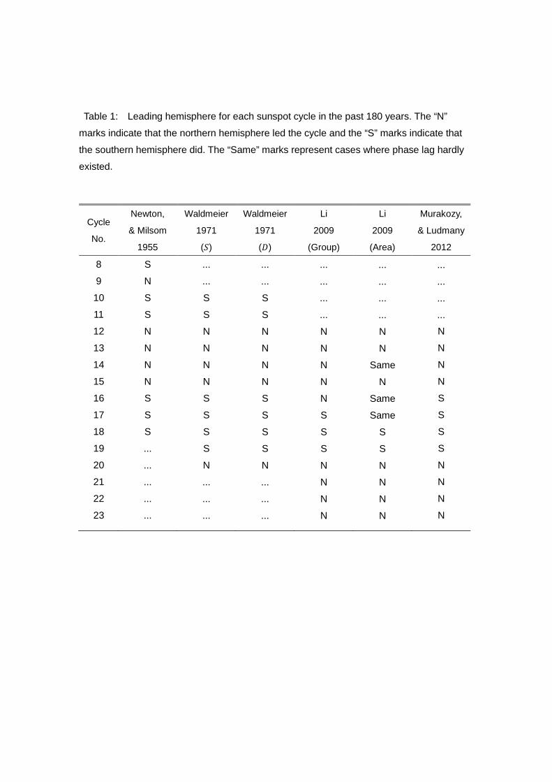
Table 1: Leading hemisphere for each sunspot cycle in the past 180 years. The “N” marks indicate that the northern hemisphere led the cycle and the “S” marks indicate that the southern hemisphere did. The “Same” marks represent cases where phase lag hardly existed.

Cycle

No.

Newton,

& Milsom

1955

Waldmeier

1971

(𝑆𝑆)

Waldmeier

1971

(𝐷𝐷)

Li

2009

(Group)

Li

2009

(Area)

Murakozy,

& Ludmany

2012

8 9 10 11 12 13 14 15 16 17 18 19 20 21 22 23

S N S S N N N N S S S ... ... ... ... ...

...

... S S N N N N S S S S N ... ... ...

...

... S S N N N N S S S S N ... ... ...

...

...

...

... N N N N N S S S N N N N

...

...

...

... N N

Same N

Same Same

S S N N N N

...

...

...

... N N N N S S S S N N N N

Figure 1: Time evolution of the radial magnetic fields 𝐵𝐵𝑟𝑟 for the symmetric (𝐵𝐵𝑠𝑠, solid line) and anti-symmetric (B^a, dashed line) components at the north pole. The initial conditions of the amplitude and phase for each component are the same value in this case, where 𝜂𝜂𝑆𝑆𝑆𝑆𝑅𝑅 = 2.6×1012 cm2s-1.

Figure 2: Time evolution of the phase difference 𝛥𝛥𝛥𝛥 for the 22 different runs of various initial conditions within the range −180° ≤ 𝛥𝛥𝛥𝛥 ≤ 180°.

Figure 3: Time evolution of the magnetic field after falling into the attractor for 𝛥𝛥𝛥𝛥 = 90°. Top panel: (dashed line) the total number of grids where the toroidal magnetic field exceeds the critical intensity for the magnetic buoyancy effect: (solid line) the difference in grid number for magnetic buoyancy effects operated between the northern and southern hemispheres. Second panel: the grid number of magnetic buoyancy in the northern (solid

lien) and southern (dashed line) hemispheres. Third panel: the time evolution of the radial

magnetic field 𝐵𝐵𝑟𝑟 at the north pole 𝐵𝐵𝑟𝑟𝑁𝑁𝑁𝑁𝑟𝑟 (solid line) and at the south pole 𝐵𝐵𝑟𝑟𝑆𝑆𝑁𝑁𝑆𝑆 (dashed line). Fourth panel: the time evolution of the radial magnetic field 𝐵𝐵𝑟𝑟 of the symmetric (solid line) and anti-symmetric (dashed line) components at the north pole as in Figure 1. Bottom

contour maps: the contour of the vector potential 𝐴𝐴 at the times corresponding to the vertical dashed lines in the top three panels. The solid and dashed contours represent magnetic field lines directed by arrows. The portion bounded by thick line corresponds to the simulation box. The contours of potential field in outside of the simulation box are also plotted.

Figure 4: Time evolutions of the magnetic field after falling into the attractor for 𝛥𝛥𝛥𝛥 = −90°. The descriptions for each panel and the contour maps are the same as those in Figure 3.

Figure 5: Time evolution of the magnetic ratio 𝜒𝜒 at different 𝑅𝑅𝑅𝑅 values. (A) 𝑅𝑅𝑅𝑅 =

7.65×103, (B) 𝑅𝑅𝑅𝑅 = 6.80×103, (C) 𝑅𝑅𝑅𝑅 = 6.12×103, (D) 𝑅𝑅𝑅𝑅 = 6.09×103, (E) 𝑅𝑅𝑅𝑅 = 6.06×

103, (F) 𝑅𝑅𝑅𝑅 = 6.03×103, (G) 𝑅𝑅𝑅𝑅 = 5.97×103, (H) 𝑅𝑅𝑅𝑅 = 5.83×103, (I) 𝑅𝑅𝑅𝑅 = 5.56×103, and (J) 𝑅𝑅𝑅𝑅 = 5.10×103, respectively.

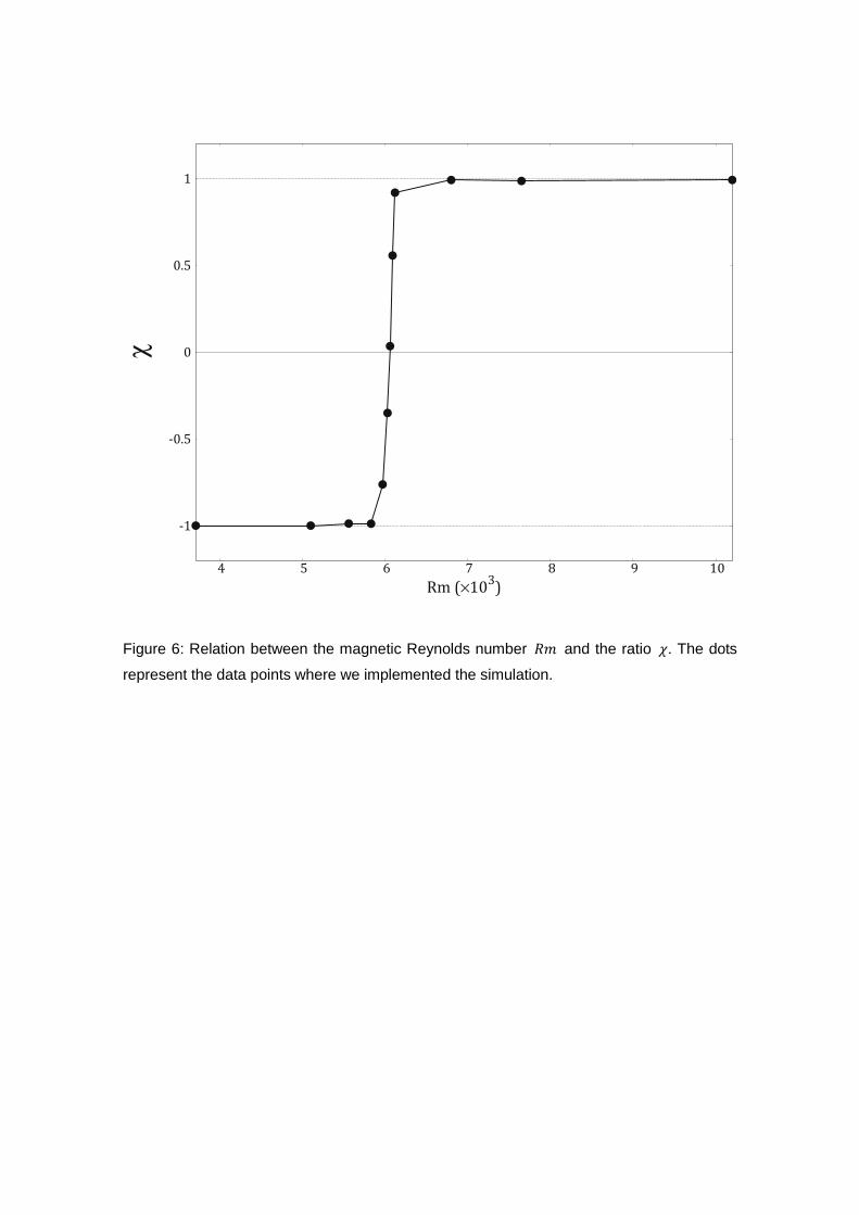
Figure 6: Relation between the magnetic Reynolds number 𝑅𝑅𝑅𝑅 and the ratio 𝜒𝜒. The dots represent the data points where we implemented the simulation.

Figure 7: Relationship between the lag time 𝛥𝛥𝑡𝑡𝑙𝑙𝑎𝑎𝑙𝑙 and the ratio 𝜒𝜒. The dots represent the

data points where we implemented the simulation.

Figure 8: Mathematical experiment for the solar cycle modulation. Upper panel: Variations of the absolute value of the magnetic field on the northern (solid) and southern (dashed) hemispheres. Lower panel: Variations of the symmetric (solid) and anti-symmetric (dashed) magnetic components. The envelope curves for each magnetic component are also plotted (dotted lines).