Proceedings of the 3rd International Conference on Mechanical Engineering and Mechatronics

Prague, Czech Republic, August 14-15, 2014

Paper No. 139

139-1

Simulation, Prediction and Compensation of Transient Thermal Deformations of a Reciprocating Linear Slide for

F8S Motion Error Separation

E.H.K. Fung, N.J. Hou, H.F. Yu, W.O. Wong The Hong Kong Polytechnic University, Department of Mechanical Engineering

Hung Hom, Kowloon, Hong Kong, China

mmhkfung@polyu.edu.hk; hounengjie@gmail.com; 11900610R@connect.polyu.hk;

mmwowong@polyu.edu.hk

Abstract - This study first introduces the prediction of the transient thermal-elastics deformation and

the temperature distribution due to friction force derived from the reciprocating motion between the

moving parts of a simulation slide model. The FEM results are incorporated into the input motion

errors to generate the simulated sensor data for evaluating the Integrated Sensing System (ISS). The

procedure for the thermal error compensation is proposed as a pre-processor for the F8S based error

separation method. Simulation results show that the F8S based ISS is capable of predicting and

compensating the transient thermal errors in a reciprocating linear slide.

Keywords: Active error compensation, Linear slide, F8S method, Thermal deformation, Straightness,

Roll, Yaw, Profile, On-machine error separation.

1. Introduction Thermal errors (Bryan, 1990; Ramesh et al., 2010) are frequently the biggest problem faced by

production engineers as they can account for around 50% of the total positional error of a machine

tool. They arise from a combination of internally generated heat such as friction and motor and

environmental influences, which unless controlled properly can result in large positional errors (Lee et

al., 2003).

In 2010, an efficient method called Fourier-Eight Sensor (F8S) method was proposed by Fung,

et al. (2010), to measure the motion errors during machining. The method (Fung et al., 2010; Fung et

al., 2014) successfully separates the motion errors into straightness, yawing and rolling errors.

Recently, the ISS (Fung et al., 2012; Fung et al., 2013) was designed to reveal the thermal effects and

the procedure of thermal error compensation. In this method (Fung et al., 2013), steady state thermal

deformation of the table was established using three temperature sensors. However, the transient

thermal effect was not fully considered in the simulation study.

The FEM-based transient thermal-structural analysis of a slide model is described in section 2.

The FEM simulation procedure is also outlined in this section. Preparation of simulated sensor data is

presented in section 3. Error separation using ISS is given in section 4. Simulation results are

presented in section 5. Concluding remarks are made in section 6.

2. FEM-based Transient Thermal-structural Analysis In this work, a 3D model of the transient thermal-structural simulation was developed on top of

a commercial FEM program called ANSYS® WorkbenchTM

2.0. It is used to analyze the phenomenon

of heat dissipation in the workpieces and its influence on part deformation. The developed system

allows users:

I. To create 3D FEM models of the workpiece configurations;

II. To apply appropriate machine boundary conditions and loads ;

III. To perform transient thermal simulation with nonlinear phenomena involving dynamic effects

and complex behaviors; and

IV. To perform transient structural simulation for the reciprocating motion of a linear slide.

139-2

The FEM-based analysis using ANSYS takes the following steps.

Step 1 - Choose Analysis System

In this study, two analysis systems, i.e. Transient Structural Analysis and Transient Thermal

Analysis are used.

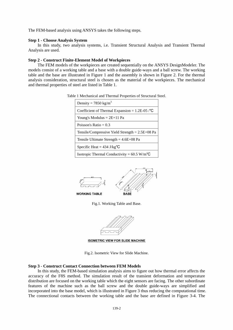
Step 2 - Construct Finite-Element Model of Workpieces

The FEM models of the workpieces are created sequentially on the ANSYS DesignModeler. The

models consist of a working table and a base with a double guide-ways and a ball screw. The working

table and the base are illustrated in Figure 1 and the assembly is shown in Figure 2. For the thermal

analysis consideration, structural steel is chosen as the material of the workpieces. The mechanical

and thermal properties of steel are listed in Table 1.

Table 1 Mechanical and Thermal Properties of Structural Steel.

Density = 7850 kg/m3

Coefficient of Thermal Expansion = 1.2E-05 /℃

Young's Modulus = 2E+11 Pa

Poisson's Ratio = 0.3

Tensile/Compressive Yield Strength = 2.5E+08 Pa

Tensile Ultimate Strength = 4.6E+08 Pa

Specific Heat = 434 J/kg℃

Isotropic Thermal Conductivity = 60.5 W/m℃

Fig.1. Working Table and Base.

Fig.2. Isometric View for Slide Machine.

Step 3 - Construct Contact Connection between FEM Models

In this study, the FEM-based simulation analysis aims to figure out how thermal error affects the

accuracy of the F8S method. The simulation result of the transient deformation and temperature

distribution are focused on the working table which the eight sensors are facing. The other subordinate

features of the machine such as the ball screw and the double guide-ways are simplified and

incorporated into the base model, which is illustrated in Figure 3 thus reducing the computational time.

The connectional contacts between the working table and the base are defined in Figure 3-4. The

139-3

salient semi-circular feature of the base representing the ball screw is defined to have frictional

contact with the working table with friction coefficient 0.8. The double salient rectangular features of

the base representing the double guide-ways are defined to have frictional contacts with the working

table with friction coefficient 0.16. Other contact faces between the working table and the base are

defined as frictionless connections.

Step 4 - Generate ANSYS Meshing

To balance the efficiency and accuracy requirements, the adaptive mesh size of 80mm and

15mm are used for the base model and the working table model respectively.

Step 5 - Define Boundary Condition

In this study, a fixture-workpiece is defined by fastening the bottom surface of the base model to

facilitate simulation containing a dynamic motion. The environment temperature is kept at 22oC with

a convective heat transfer coefficient of 25W/m2K. The initial temperature of all models is defined as

22oC. Heat radiation to the surrounding is ignored.

Step 6 - Create Load and Motion as a Function of Time

A back-and-forth or reciprocating motion of ± 1mm/s along the X-direction is created on the

working table. To produce a frictional force, a dummy normal pressure is applied on the working table

along Y-direction. The simulation time is 14400s (4 hours) with 144 number of steps (1 step = 100s)

which allows the temperature to reach an equilibrium value. At this point, the heat generated by

frictional force is equal to that transferred to the surrounding environment.

Step 7 - Perform Transient Thermal-Structural Analysis

For determining the time-varying deformation and temperature distribution in the workpieces

during machining process, the Transient Thermal-Structural Analysis is conducted following the

procedure given in (Expertfea, 2013).

Step 8 - Postprocess Numerical Results

The numerical results are then processed by the Report Generator Module and presented in the

form of colored contours and graphs showing the transient temperature distribution and part

deformations at specific nodal locations designated by the ISS.

Step 9 - Define Temperature Sensor Placement For each thermal mode, it is always desirable to place the temperature sensors according to the

following rules:

(1) Close to the extreme values of the dominant temperature fields or,

(2) Close to the heat flux sources.

The temperature sensor location is shown in Figure 5.

Step 10 - Define Eight Locations Facing the Displacement Sensors

The stationary sensor stage is fixed to the table base at specific location. The arrangement of

displacement sensors on sensor stage follows the design requirement of the F8S method. All these

sensors must face the target profile (Figure 6) of the machine during data collection. The target profile

is set to be on one side of the machine. As shown in Figure 8, the sensor location is configured as

follows: Total test section length L=60mm; P1 is taken to be the zero position or the reference point;

distance between P1 and P2, l2=15.6mm; distance between P1 and P4 or P6 and P7, l4=33.8mm; distance

between the lower sensor row and the rolling axis, h1 is 4mm; distance between the upper sensor row

and the rolling axis, h2 is 44mm.

139-4

Fig. 3. Contract Surface between working table and base (2 nos. guideway).

Fig. 4. Contact Surface between working table and base (ball screw).

Fig. 5. Temperature Sensor Location.

Fig. 6. Profile Facing Sensor Stage.

3. Preparation of Simulated Sensor Data The simulation program (Fung et al., 2010; Fung et al., 2014) combines the predefined

f1(θ), f2(θ), the randomly generated Z̃(θ), γ(θ) and ω(θ), to obtain S1, S2, …, S8 as shown in Figure

7. Then, the thermal deformation ∆f1(θ), ∆f2(θ) are added to S1, S2, …, S8 along L1 and L2

respectively as indicated in Figure 6, to create the simulated sensor signals S1T, S2T, …., S8T.

3.1. Determination of ∆𝐟𝟏(𝛉) 𝐚𝐧𝐝 ∆𝐟𝟐(𝛉)

The values of thermal deformation at t = 100s, 2500s, 4900s, 7300s and 9700s for P1’, P2’, …, P8’

are found by ANSYS as described in step 10 of section 2. For the transient study, the thermal

deformations along L1 and L2 are considered for five motions beginning with t = 100s, 2500s, 4900s,

139-5

7300s and 9700s. The sensors will face the same locations at the profile at the start of each motion.

The profile changes are assumed to be constant for the 60mm travel. For a particular time, say t =

100s, the values of thermal deformations along L1 and L2 are found by linear interpolations based on

the known deformation at the eight points. Interpolation is used to find the approximate profile ∆f1

and ∆f2 at 301 points, which approximates a complicated function by a simple function.

3.2. Formation of S1T, S2T, …, S8T

The predefined f1(θ), f2(θ), Z̃(θ), γ(θ) and ω(θ), which are shown in Figure 7, are combined

together with thermal deformation ∆f1(θ), ∆f2(θ) to create the simulated sensor signals

S1T, S1T, … , S8T. The magnitudes of , Z̃(θ), γ(θ) and ω(θ) are chosen according to some industrial

guidelines.

Fig. 7. Predefined inputs (4900s).

The simulated data is now ready for testing the performance of the Integrated Sensing System (ISS).

4. Error Separation Using ISS

The estimated values of thermal deformations at P1’, P2’, …, P8’, are used to generate the

approximate ∆f1′, ∆f2′ along L1 and L2 respectively for the five starting times t= 0s, 100s, 2500s,

4900s, 7300s by interpolation. The estimated values are obtained by equation (1) with coefficients

found by Linear Square Regression. The calculated ∆f1′, ∆f2′ are subtracted from S1T, S2T, … , S8T

to get the new sensor data S1𝑇 + , S2𝑇

+ , … , S8𝑇 + . The F8S method is then applied to process

S1𝑇 + , S2𝑇

+ , … , S8𝑇 + to obtain the profiles of f1

+, f2+ and the motion errors Z

+, γ+ 𝑎𝑛𝑑 𝜔+.

4.1. Least Square Regression The thermal error model of the table is derived to relate the temperature changes collected at the

sensor locations (ΔT1, ΔT2 and ΔT3) to the estimated thermal deformation of specific points, i.e. P1’,

P2’, …, P8’ on that component. The relationship can be represented in the following form:

[D] = [∆T][A] (1)

where [D] denotes the estimated thermal deformation matrix for P1’, P2’ to P8’, [∆T] is the measured

temperature change matrix, and [A] is the coefficient matrix found by Least Square Regression using

temperatures and deformations obtained at t = 100s, 200s, 300s, …., 10800s.

From equation (1), it can be shown that

]D[]T[]}T[]T{[]A[ T1T �

where [∆T̅] and [D̅] are the temperature change matrix and the thermal deformation matrix obtained

by thermal-structural analysis.

139-6

4.2. Estimation of Thermal Deformation at P1’, P2’, …, P8’ With the known values of [A] in the above, the estimated deformations at P1’, P2’, …, P8’, are

found using [D] = [∆T][A] where [∆T] is the temperature matrix derived from the readings T1, T2,

T3.

4.3. Estimated ∆𝐟𝟏′ , ∆𝐟𝟐

′ for Thermal Error Compensation

The linear interpolation is applied to determine ∆f1′, ∆f2

′ along L1 and L2 using ∆f1′ and ∆f2

′ at

P1’, P2’, …, P5’ and P6’, …, P8’ respectively. The effects ∆f1′ , ∆f2

′ are subtracted from

S1𝑇 , S2𝑇 , … . , S8𝑇 to get the new sensor data S1𝑇+ , S2𝑇

+ , … . , S8𝑇+ for error seperation by F8S.

4.4. Fourier-Eight-Sensor Method (Fung et al., 2010 & 2014)

Fig. 8. Sensor Configuration.

Figure. 8 shows the sensor stage used in F8S method which involves eight displacement sensors

from P1 to P8 . P1’ to P8’ are the locations on the working plane which face the sensors P1 to P8

respectively (Figure 6). f1 and f2 are the profiles of the working plane at ambient temperature facing

the lower and upper row sensors respectively. Z is the straightness motion error of the slide; γ

and ω are the yawing and rolling motion errors of the slide respectively. The F8S method (Fung et al.,

2010; Fung et al., 2014) is used to obtain the profiles f1 and f2 by using data histories of the eight

sensors assuming zero thermal deformation. Other errors can be separated through simple equations

based on the calculated profile functions. The procedure for determining f1, f2, Z, γ and ω of a linear

slide can be found in (Fung et al., 2010; Fung et al., 2014).

5. Simulation Results 5.1. ANSYS Results on Temperature Distribution

The transient temperature distribution of the working table for t=100s, 2500s, 4900s, 7300s and

9700s, are obtained by ANSYS Transient Thermal-Structural Analysis Simulation. The temperature

responses of T1, T2, T3 are found by this simulation. Typical temperature distribution at t = 4900s

and the response of T1 for 100s < t < 14400s are shown in Figure 9 and 10 respectively.

Fig. 9. Temperature Distribution at 4900s.

139-7

Fig. 10. Temperature Response of T1.

5.2. ANSYS Results on Thermal Deformations

The detected transient thermal deformations of eight points (P1’ to P8’) facing the eight distance

sensors P1 to P8 of the ISS, i.e. ∆𝑓1(𝑃1′), ∆𝑓1(𝑃2

′), … , ∆𝑓2(𝑃7′), ∆𝑓2(𝑃8

′), are obtained by ANSYS

Transient Thermal-Structural Analysis simulation. The estimated values i.e.

∆𝑓1(𝑃1′), ∆𝑓1(𝑃2

′), … , ∆𝑓2(𝑃7′), ∆𝑓2(𝑃8

′), are calculated based on the measured temperature changes

(ΔT1, ΔT2 and ΔT3) using equation (1). Typical results for ∆𝑓1(𝑃1′) and ∆𝑓1

′(𝑃1′) at location P1’ are

shown in Figure 11.

Fig. 11. Comparison between Δf1’(P1’) and Δf1(P1’).

5.3. Error Separation based on F8S method

The estimated results with thermal error compensation (Case 2) f1+ f2

+, Z

+, γ

+ and w

+ and the

results without thermal error compensation (Case 1) f1*, f2*, Z*, γ* and w* are obtained by F8S

method. At t = 4900s, Z, Z+

and Z* are compared in Figure 12(a) while w, w+ and w* are compared in

Figure 12(b). Table 2 lists the result summary.

0.0000E+00

5.0000E-06

1.0000E-05

1.5000E-05

2.0000E-05

2.5000E-05

3.0000E-05

3.5000E-05

100 1200 2300 3400 4500 5600 6700 7800 8900 10000

Def

orm

atio

n (

m)

Time (s)

Thermal deformation at P1'

P1'

P1"

Δf1

Δf1’

139-8

(a)

(b)

Fig. 12. (a) Straightness Error 𝑍 at 4900s; (b) Rolling Error 𝜔 at 4900s.

The ANSYS simulation results show that the temperature of the table rose by about 6oC to 9

oC

and becomes steady at 3 hrs. It is found that the temperature responses at detected locations show

similar trends and the increased values are similar to those reported by Rai and Xirouchakis (2009).

The maximum thermal deformation is 2.90x10-5

m at P6’ and P7’ along the travel. It is observed that

the ANSYS values and the estimated values at all sensor detected locations show similar trend over

the entire reciprocating motion.

At t = 4900s, it is found that the calculated results without thermal compensation for the profile

and yawing f1∗ , f2

∗ and γ∗ do not show any significant deviation from their pre-defined values

f1 , f2 and γ and the estimated ones with thermal compensation f1+ , f2

+ and γ+. However, the

average difference for Z and w are increased by 36 and 29 times respectively when the thermal effects

are not taken into account. On the other hand, the estimated Z+ and ω+ show good agreement with

the pre-defined values when the thermal deformations are considered by using the ISS.

Table 2. Maximum and Average Differences for Case 1 and Case 2 (t = 4900s).

Parameters for comparison Case 1

without thermal effect compensation

Case 2

With thermal effect compensation

M-dif of f1 (mm) 54.22 10 68.01 10

Ave-dif of f1 (mm) 52.04 10 63.78 10

M-dif of f2 (mm) 58.38 10 55.8 10

Ave-dif of f2 (mm) 51.24 10 68.82 10

M-dif of motion (mm) 22.61 10 48.26 10

Ave-dif of motion (mm) 22.61 10 47.26 10

M-dif of yaw( deg) 59.29 10 41.83 10

Ave-dif of yaw (deg) 59.19 10 41.82 10

M-dif of roll (deg) 42.15 10 41.13 10

Ave-dif of roll (deg) 41.12 10 63.86 10

M-dif = max[abs(predefined data – calculated data)]

Ave-dif = sum[abs(predefined data – calculated data)]/301

6. Concluding Remarks An Integrated Sensing System (ISS) is successfully proposed to separate the profiles, the yaw

139-9

and the roll errors of a reciprocating linear slide under the effects of transient thermal deformations.

The system consists of eight displacement and three temperature sensors. Implementation requires the

three major steps:

(1) Estimation of thermal deformations at eight sensor detected locations based on the three

temperature sensor outputs.

(2) Estimation of the quasi-steady deformation profiles along the scanning direction for a

particular travel based on the values at the eight detected locations in (1).

(3) Subtraction of results in (2) from the sensor outputs followed by error separation using F8S

method.

A FEM-based transient thermal-structural simulation using ANSYS is used to generate the

transient thermal deformation data for verifying the above implementation. The linear slide model

consists of a reciprocating table and a fixed base with rectangular and semi-circular protruding

features representing the guide-ways and the ball screw respectively. Simulation results verify that the

ISS system performs well under both transient and steady state conditions. The prediction errors for

straightness and roll motion have been significantly reduced by about 30 times when the thermal error

compensation is incorporated. The efficiency and availability of the machine can be greatly improved

as production can be extended to include the three-hour warm-up period.

Acknowledgements

The authors would like to thank The Hong Kong Polytechnic University for the financial support

(Project No. G-YK13) towards this work. Thanks are also due to Mr. CH Cheung, Mr. CM Yu and Mr.

WC Mak for their assistance in generating some results presented herein.

References

Bryan, J. (1990). International Status of Thermal Error Research. CIRP Annals – Manufacturing

Technology, 39(2), 645-656.

Expertfea (2013). Finite Element Analysis Hints and ANSYS Workbench Tutorial – Transient

Structural FEA of Heat Generated Between a Piston and a Cylinder. Retrieved from

http://expertfea.com/

Fung, E.H.K., Hou, N.J., Zhu, M., Wong, W.O. (2012). A Novel Integrated Sensing System (ISS) for

Monitoring Motion Errors of a Precision Linear Slide. “In Proceedings of ASME 2012

International Mechanical Engineering Congress and Exposition,” Texas, Nov 2012, pp. 17-24.

Fung, E.H.K., Hou, N.J., Zhu, M., Wong, W.O. (2013) .A Novel Method for On-Machine

Determination of Slide Motion Errors Considering Thermal Effects. Applied Mechanics and

Materials, 42, 157-162.

Fung, E.H.K., Zhu, M., Zhang, X.Z., Wong, W.O. (2010) .An Improved Fourier Eight-Sensor (F8S)

Method for Separating Straightness, Yawing and Rolling Errors of a Linear Slide. “In

Proceedings of ASME 2010 International Mechanical Engineering Congress and Exposition,”

Canada, Nov 2010, pp. 371-378.

Fung, E.H.K., Zhu, M., Zhang, X.Z., Wong, W.O. (2014) .A Novel Fourier-Eight-Sensor (F8S)

Method for Separating Straightness. Yawing and Rolling Motion Errors of a Linear Slide,

Measurement, 47, 777-788.

Lee, S.K., Yoo, J.H., Yang, M.S. (2003). Effect of Thermal Deformation on Machine Tool Slide Guide

Motion. Tribology International, 36(1), 41-47.

Rai, J.K., Xirouchakis, P. (2009). FEM-based Prediction of Workpieces Transient Temperature

Distribution and Deformation during Milling. International Journal of Advanced

Manufacturing Technology, 42, 429-449.

Ramesh R., Mannan, M.A., Poo, A.N. (2000). Error Compensation in Machine Tools - a Review, Part

II: Thermal Errors, International Journal of Machine Tools & Manufacturing, 40, 1257-1284.