SIMULATION ON INTERFEROMETRIC FIBER OPTIC …etd.lib.metu.edu.tr/upload/1253657/index.pdf · Öz...
99
SIMULATION ON INTERFEROMETRIC FIBER OPTIC GYROSCOPE WITH AMPLIFIED OPTICAL FEEDBACK A THESIS SUBMITTED TO THE GRADUATE SCHOOL OF NATURAL AND APPLIED SCIENCES OF THE MIDDLE EAST TECHNICAL UNIVERSITY BY BAŞAK SEÇMEN IN PARTIAL FULLFILMENT OF THE REQUIREMENTS FOR THE DEGREE OF MASTER OF SCIENCE IN THE DEPARTMENT OF PHYSICS SEPTEMBER 2003
-
Upload
nguyennhan -
Category
Documents
-
view
224 -
download
0
Transcript of SIMULATION ON INTERFEROMETRIC FIBER OPTIC …etd.lib.metu.edu.tr/upload/1253657/index.pdf · Öz...
SIMULATION ON INTERFEROMETRIC FIBER OPTIC GYROSCOPE WITH AMPLIFIED OPTICAL FEEDBACK
A THESIS SUBMITTED TO THE GRADUATE SCHOOL OF NATURAL AND APPLIED SCIENCES
OF THE MIDDLE EAST TECHNICAL UNIVERSITY
BY
BAŞAK SEÇMEN
IN PARTIAL FULLFILMENT OF THE REQUIREMENTS FOR THE DEGREE OF
MASTER OF SCIENCE IN
THE DEPARTMENT OF PHYSICS
SEPTEMBER 2003
ABSTRACT
SIMULATION ON
INTERFEROMETRIC FIBER OPTIC GYROSCOPE
WITH AMPLIFIED OPTICAL FEEDBACK
Seçmen, Başak
M.S., Department of Physics
Supervisor: Assoc. Prof. Dr. Serhat Çakır
September 2003, 87 Pages
Position and navigation of vehicle in two and three dimensions have been
important as being advanced technology. Therefore, some system has been evaluated
to get information of vehicle’s position. Main problem in navigation is how to
determine position and rotation in three dimensions. If position and rotation is
determined, navigation will also be determined with respect to their initial point.
There is a technology that vehicle velocity can be discovered, but a technology that
rotation can be discovered is needed. Sensor which sense rotation is called
gyroscope. If this instrument consists of optical and solid state material, it’s defined
by Fiber Optic Gyroscope (FOG).
iii
There are various studies in order to increase the sensitivity of fiber optic
gyroscopes, which is an excellent vehicle for sensing rotation. One of them is
interferometric fiber optic gyroscope with amplified optical feedback (FE_FOG). In
this system, a feedback loop, which sent the output pulse through the input again, is
used. The total output is the summation of each interference and it is in pulse state.
The peak position of the output pulse is shifted when rotation occurs. Analyzing this
shift, the rotation angle can be determined.
In this study, fiber optic gyroscopes, their components and performance
characteristics were reviewed. The simulation code was developed by VPIsystems
and I used VPItransmissionMakerTM software in this work. The results getting from
both rotation and nonrotation cases were analyzed to determine the rotation angle
and sensitivity of the gyroscope.
Key words: Fiber optic gyroscope, Sagnac interferometer, EDFA, Amplified
feedback loop, simulation.
iv
ÖZ
YÜKSELTİLMİŞ OPTİKSEL GERİ BESLEME DÖNGÜLÜ
İNTERFEROMETRİK FİBER OPTİK JİROSKOP SİMÜLASYONU
Seçmen, Başak
Master, Fizik Bölümü
Tez Yöneticisi: Doç. Dr. Serhat Çakır
Eylül 2003, 87 Sayfa
Gelişen teknolojiye paralel olarak araçların veya cisimlerin iki ve üç boyutlu
uzayda konum ve pozisyonunun bilinmesi önem kazanmıştır. Bu yüzden, bu
pozisyonlamanın yapılabilmesi için çeşitli sistemler geliştirilmiştir. Yer tayinindeki
en temel problem, üç boyutlu uzayda pozisyon ve açısal dönmenin nasıl
ölçüleceğidir. Eğer bu nicelikleri belirleyebilirsek, bilinen bir başlangıç noktasına
göre aracın hareket vektörünü ve konumunu hesaplayabiliriz. Aracın hız vektörünü
belirleyebilecek teknoloji mevcuttur, fakat dönmeyi algılayacak teknolojiye ihtiyaç
duyulmaktadır. Dönmeyi algılayan sensörlere jiroskop denir. Sagnac
İnterferometrenin keşfi ve yarı iletken teknolojisinin gelişmesiyle, jiroskoplar
tamamen optiksel ve yarı iletken materyallerden oluşan bir cihaza dönüşmüştür. Bu
cihaza Fiber Optik Jiroskop (FOG) denmektedir.
v
Açısal dönmeyi ölçmek için mükemmel bir cihaz olan fiber optik jiroskopun
duyarlılığını artırmak için çeşitli çalışmalar yapılmaktadır. Bunlardan biri de
yükseltilmiş geri bildirim döngülü interferometrik fiber optik jiroskoptur. Bu
sistemin çalışması jiroskoptan alınan çıktının tekrar girişten gönderilmesini sağlayan
bir döngü oluşturularak darbeler elde etme esasına dayanmaktadır. Jiroskobun dönme
açısına bağlı olarak sapma gösteren bu darbeler incelenerek dönme miktarı belirlenir.
Bu çalışmada fiber optik jiroskopların özellikleri incelendi. VPIsystems
tarafından geliştirilen VPItransmissionMakerTM yazılımı kullanılarak yükseltilmiş
geri bildirim döngülü interferometrik fiber optik jiroskop simülasyonu yapıldı.
Jiroskobun hareketsiz konumunda ve çeşitli açılarda dönmesi durumlarında elde
edilen sonuçlar karşılaştırılarak dönme açısı tayini yapıldı ve duyarlılığı incelendi.
Anahtar kelimeler: Fiber optik jiroskop, Sagnac interferometre, EDFA,
Yükseltilmiş geri besleme döngüsü, simülasyon.
vi

ACKNOWLEDGMENTS
I would like to acknowledge gratefully to my supervisor Assoc. Prof. Dr.
Serhat Çakır for his guidance, support and encouragements during this thesis. I
would also like to thank to Dr. Ali Alaçakır for his suggestions and comments. I am
also grateful to my friends, Başak Ballı and F. Feza Büyükşahin for their helps and
suggestions. Finally, I wish to thank my family for their supports and
encouragements.
vii

TABLE OF CONTENTS
ABSTRACT…………………………………………………………………….. iii
ÖZ……………………………………………………………………..………… v
ACKNOWLEDGEMENTS…………………………………………………… vii
TABLE OF CONTENTS……………………………………………………… viii
LIST OF FIGURES…………………………………………………………… xi
CHAPTERS
1. OVERVIEW OF FIBER OPTIC GYROSCOPES….……………. 1
1.1 Introduction………………………………………………….. 1
1.1.1 Review of Wave Physics……………………………… 3
1.1.2 Interference of Waves…………………………………. 5
1.2 Basic Principle of The Fiber Optic Gyroscope……………… 11
1.2.1 Sagnac Effect…………………………………………. 11
1.2.2 Bias Modulation…………………….………………… 14
2. FOG CONSTRUCTION AND COMPONENTS………………… 19
2.1 Reciprocity…………………………………………………. 19
2.2 Fiber Coil……………………………………...……………. 21
2.3 Light Source………………………..……………………….. 21
2.4 Coupler…………………………….…….…………………. 23
2.5 Phase Modulators……………………..……………………. 24
2.6 Detector…………………………………………………….. 26
3. GYRO PERFORMANCE…………………………………………. 27
3.1 Noise……..…………………………………………………. 27
3.1.1 Shot Noise………………………………………… 27
3.1.2 Johnson Noise…………………………………….. 28
3.1.3 Thermal Phase Noise……………………………... 28
3.1.4 Relative Intensity Noise…………………………... 28
viii
3.2 Bias Stability……………………………………………….. 28
3.2.1 Bias Error Mechanisms…………………………… 28
3.2.1.1 Modulator Error………………………………… 28
3.2.1.1.A) Nonlinearity……………………….… 28
3.2.1.1.B) Intensity Modulation………………… 29
3.2.1.2 Secondary Waves……………………………….. 29
3.2.1.3 Nonreciprocal Effects……………………...…… 29
3.3 Input Axis Alignment………………………………………. 30
3.4 Deadzone (Lock-In)………………………………………… 31
3.5 Scale Factor Stability……………………………………….. 31
4. SIMULATION ON INTERFEROMETRIC FIBER
OPTIC GYROSCOPE WITH AMPLIFIED OPTICAL
FEEDBACK (FE-FOG)…………………………………………….. 32
4.1 Properties of Simulation Program, VPItransmissionmakerTM 32
4.2 Signal Representations……………………………………… 33
4.3 Global Variables……………………………………………. 33
4.4 Interferometric Fiber Optic Gyroscope
with Amplified Optical Feedback (FE-FOG)…………….. 35
4.5 Configuration of A FE_FOG……………………………….. 36
4.6 Theory……………………………………….……………… 37
4.7 Simulations And Discussions……………….……………… 40
4.8 Modules Used in the Schematic………….………………… 42
4.8.1 LaserCW……………….………….……………… 42
4.8.2 X Coupler And X Coupler Bi-Directional……….. 43
4.8.3 Phase Shift……………………………………….. 43
4.8.4 Sine Generator (Electrical) …………...…….…… 43
4.8.5 Multiple Output Connector (Fork) …...………….. 44
4.8.6 Modulator Phase…………………………………. 44
4..8.7 Photodiode (Pin)………………………………… 44
4.8.8 Time Domain Fiber….…………………………… 45
4.8.9 Ideal Amplifier with Wavelength Independent Gain 46
4.9 Results……………………………………………………… 47
ix
5. CONCLUSION………….……………………………...…………… 55
REFERENCES………………………………………………………………… 57
APPENDICES
A. MODULES USED IN THE SIMULATION …………………….. 60
A.1 LaserCW ……………………..……………………….…… 60
A.2 X Coupler……………………………………………….…... 64
A.3 X Coupler Bidirectional…………………………………….. 66
A.4 Phase Shift………………………………………………….. 66
A.5 Sine Generator (Electrical)…………...…………………….. 69
A.6 Multiple Output Connector (Fork)…………………………. 71
A.7 Modulator Phase…………………………………………… 72
A.8 Photodiode Pin……………………………………………… 74
A.9 Null Source………………………………………………… 77
A.10 Ground……………………………………………………. 78
A.11 Time Domain Fiber………………………………..……… 79
A.12 Ideal Amplifier with Wavelength Independent Gain.……. 84
x
LIST OF FIGURES
1.1 Propagation of monochromatic wave……………………………………..….3
1.2 March-Zender Interferometer………................................................................5
1.3 Interferogram for monochromatic waves…...…………………………..…….7
1.4 Interferogram for polychromatic waves……………………………….…...…8
1.5 Gaussian spectrum of S(f) centered about f0………………………………….9
1.6 Interference fringe of coherence function for cττ >> …………….………...10
1.7 Interference fringe of coherence function for cττ ≈ ……………...………...10
1.8 Sagnac-ring interferometer…………...………………………………….….11
1.9 a) Sagnac-ring interferometer
b) Simplified calculation of the Sagnac-effect………………….………...…12
1.10 Sensitivity at various points on interferogram………………………...…….15
1.11 Method to inject relative phase shift between CW and CCW waves……….16
1.12 Sinusoidal bias modulation:
detector signal with finite Sagnac phase shift .……………………………...18
xi
2.1 Reciprocal configuration…………………………………………….………20
2.2 Reciprocal use of coupler……………………………………….………..….23
2.3 PZT modulator….…………………………………………………………...25
2.4 Electro-optic modulator ….……………………………………………...…25
3.1 Input axis alignment………………………………………...……………….30
3.2 Transfer functions for an ideal fiber gyro and
for a fiber gyro with deadzone………………………….…………………...31
4.1 Global parameters…………………………………...………………………35
4.2 Configuration of the FE_FOG……………………………………………....36
4.3 Schematic of the simulation……………………………….………………...41
4.4 Parameters of Laser CW……………………………………...……...……...42
4.5 Parameters of Sine Generator……………………………...……...………...43
4.6 Parameters of Photodiode PIN…………………………….………………...44
4.7 Parameters of Time Domain Fiber in Sagnac Loop…………………………45
4.8 Parameters of Ideal Amplifier……………………………………………….46
4.9 Output signal for φs = 0, φe = 1,9 rad………………………………………..48
xii
4.10 Later output pulses for φs = 0, φe = 1,9 rad……………………...…………..48
4.11 Output signal for φs = 0, φe = 0,6 rad………………………………………...49
4.12 Comparison between two gain values (a) 8 dB and (b) 9.3 dB
for φe = 1.24 π rad...........................................................................................49
4.13 Results for φe = 0,6 rad…………………………………...………………….51
4.14 Results for φe = 1,9 rad……………………………………..……………….52
4.15 Time shift of the output peak as the function of rotation rate with different
phase modulation φe = 0,6 rad, φe = 1,9 rad....................................................53
4.16 Comparison between (a) positive rotation φs = 20o and
(b) negative rotationφs = −20o, when φe = 1.24 π rad. ……...……………….54
A.1 Schematic of the modeled DFB CW laser…………………………......……62
A.2 Implementation of the XCouplerBi Galaxy……………………………..…67
A.3 Noise equivalent diagram of a PIN-Direct-Receiver…………………...…...76
xiii
CHAPTER 1
OVERVIEW OF FIBER OPTIC GYROSCOPES
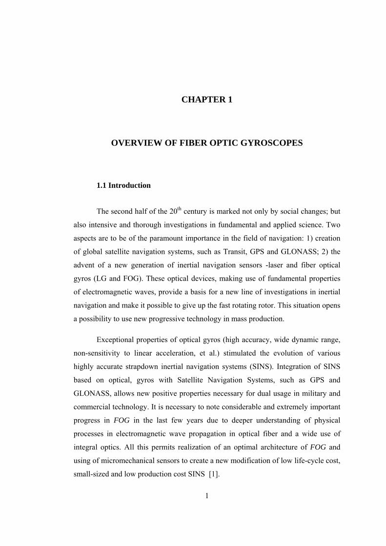
1.1 Introduction
The second half of the 20th century is marked not only by social changes; but
also intensive and thorough investigations in fundamental and applied science. Two
aspects are to be of the paramount importance in the field of navigation: 1) creation
of global satellite navigation systems, such as Transit, GPS and GLONASS; 2) the
advent of a new generation of inertial navigation sensors -laser and fiber optical
gyros (LG and FOG). These optical devices, making use of fundamental properties
of electromagnetic waves, provide a basis for a new line of investigations in inertial
navigation and make it possible to give up the fast rotating rotor. This situation opens
a possibility to use new progressive technology in mass production.
Exceptional properties of optical gyros (high accuracy, wide dynamic range,
non-sensitivity to linear acceleration, et al.) stimulated the evolution of various
highly accurate strapdown inertial navigation systems (SINS). Integration of SINS
based on optical, gyros with Satellite Navigation Systems, such as GPS and
GLONASS, allows new positive properties necessary for dual usage in military and
commercial technology. It is necessary to note considerable and extremely important
progress in FOG in the last few years due to deeper understanding of physical
processes in electromagnetic wave propagation in optical fiber and a wide use of
integral optics. All this permits realization of an optimal architecture of FOG and
using of micromechanical sensors to create a new modification of low life-cycle cost,
small-sized and low production cost SINS [1].
1
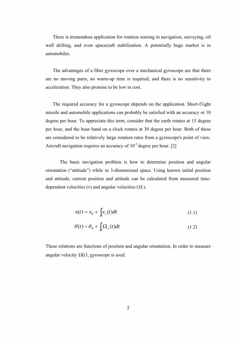
There is tremendous application for rotation sensing in navigation, surveying, oil
well drilling, and even spacecraft stabilization. A potentially huge market is in
automobiles.
The advantages of a fiber gyroscope over a mechanical gyroscope are that there
are no moving parts, no warm-up time is required, and there is no sensitivity to
acceleration. They also promise to be low in cost.
The required accuracy for a gyroscope depends on the application. Short-f1ight
missile and automobile applications can probably be satisfied with an accuracy or 10
degree per hour. To appreciate this term, consider that the earth rotates at 15 degree
per hour, and the hour hand on a clock rotates at 30 degree per hour. Both of these
are considered to be relatively large rotation rates from a gyroscope's point of view.
Aircraft navigation requires an accuracy of 10-3 degree per hour. [2]
The basic navigation problem is how to determine position and angular
orientation (“attitude”) while in 3-dimensional space. Using known initial position
and attitude, current position and attitude can be calculated from measured time-
dependent velocities (ν) and angular velocities ( Ω ).
∫+=t
x dttvxtx00 )()( (1.1)
∫ Ω+=t
x dttt00 )()( θθ (1.2)
These relations are functions of position and angular orientation. In order to measure
angular velocity , gyroscope is used. ( )tΩ
2
1.1.1 Review of Wave Physics
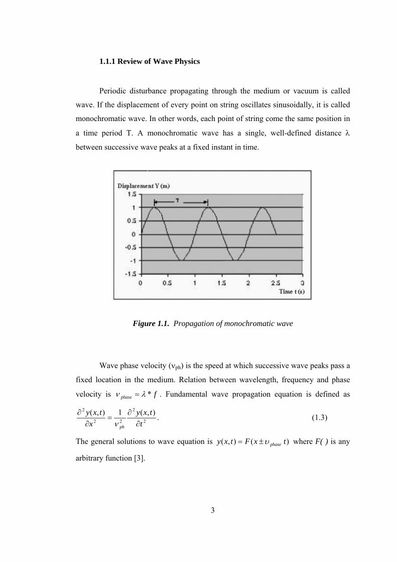
Periodic disturbance propagating through the medium or vacuum is called
wave. If the displacement of every point on string oscillates sinusoidally, it is called
monochromatic wave. In other words, each point of string come the same position in
a time period T. A monochromatic wave has a single, well-defined distance λ
between successive wave peaks at a fixed instant in time.
Figure 1.1. Propagation of monochromatic wave
Wave phase velocity (νph) is the speed at which successive wave peaks pass a
fixed location in the medium. Relation between wavelength, frequency and phase
velocity is fphase *λν = . Fundamental wave propagation equation is defined as
2
2
22
2 ),(1),(t
txyx
txy
ph ∂∂
=∂
∂ν
. (1.3)
The general solutions to wave equation is ) (),( txFtxy phaseυ±= where F( ) is any
arbitrary function [3].
3
Light wave is an electromagnetic wave. Electric (→
E ) and magnetic (→
B ) fields
oscillate simultaneously. Light waves can propagate in a vacuum or in media.
Electric field is plotted to represent wave oscillations.
Maxwell’s equations for electric and magnetic fields in vacuum;
0=⋅∇ Eρ
0=⋅∇ Bρ
(1.4)
tBE
∂∂
−=×∇ρ
ρ
tEB
∂∂
=×∇ρ
ρ00εµ (1.5)
Wave equations are obtained from curl ( ×∇ ) of equations (1.5) using identity
. EEE 2)( ∇−•∇∇=×∇×∇
2
2
002
tEE
∂∂
=∇ εµ (1.6)
2
2
002
tBB
∂∂
=∇ εµ (1.7)
Here 0µ is permeability of vacuum and 0ε is permitivity of vacuum. In fiber optic
gyroscopes light wave does not propagates through vacuum but propagates through
fused silica fiber. There are two important differences from vacuum case:
→Maxwell equations contain terms for finite charge and current density.
→Fiber permitivity isn0ε
ε = and permeability is n
0µµ = where n is the fiber
refractive index.
General solution to wave equation is
ytkxSinEtxE ))(),( 0 ω−= , where λπ /2=k , fπω 2= . (1.8)
Wave accelerates any nearby charge in the y-direction; power is deposited into
charge y-degree of freedom. This wave is said to be polarized along y.
Wave carries energy. Power carried by wave across unit area is;
20 ),(),( txEctxP ε= = ) (1.9) (22
00 tkxSinEc ωε −
4
If the wave is y_ polarized then power deposited along y-direction. If the wave is x_
and y_ polarized then power has Ex and Ey components. ( ) 22yx EEP +∝
Time-averaged power over one wave cycle is
2
)(),(20022
00EctkxSinEctxP ε
ωε =−= . (1.10)
For a single monochromatic wave, time-averaged power is independent of time and
position. [4]
2/2000 EcPP ε== (1.11)
1.1.2 Interference of Waves
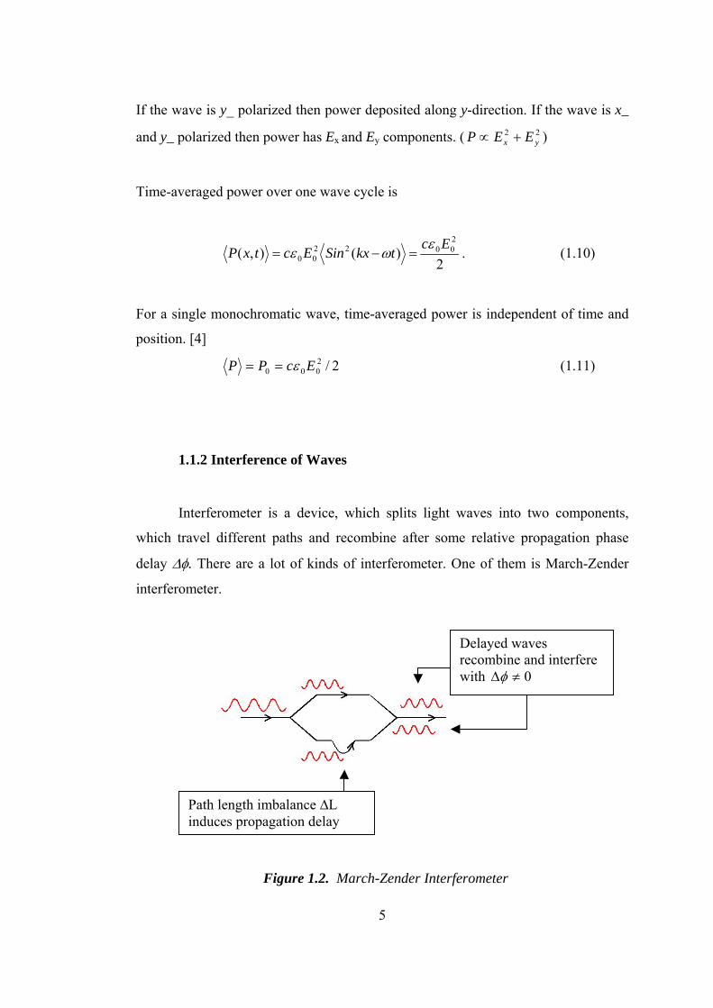
Interferometer is a device, which splits light waves into two components,
which travel different paths and recombine after some relative propagation phase
delay ∆φ. There are a lot of kinds of interferometer. One of them is March-Zender
interferometer.
Delayed waves recombine and interfere with 0≠∆φ
Path length imbalance ∆L induces propagation delay
Figure 1.2. March-Zender Interferometer
5
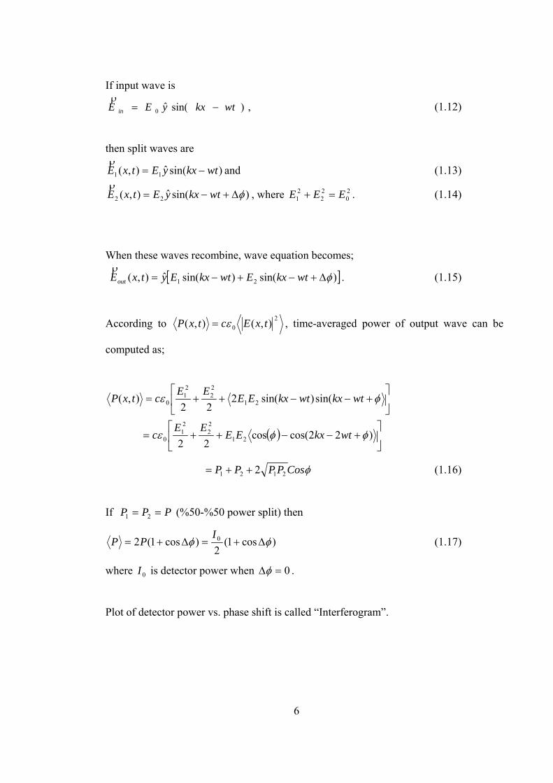
If input wave is
)sin(ˆ0 wtkxyEE in −=ρ
, (1.12)
then split waves are
)sin(ˆ),( 11 wtkxyEtxE −=ρ
and (1.13)
)sin(ˆ),( 22 φ∆+−= wtkxyEtxEρ
, where . (1.14) 20
22
21 EEE =+
When these waves recombine, wave equation becomes;
[ ])sin()sin(ˆ),( 21 φ∆+−+−= wtkxEwtkxEytxEout
ρ. (1.15)
According to 20 ),(),( txEctxP ε= , time-averaged power of output wave can be
computed as;
( ) ⎥⎦
⎤⎢⎣
⎡+−−++=
⎥⎦
⎤⎢⎣
⎡+−−++=
)22cos(cos22
sin()sin(222
),(
21
22
21
0
21
22
21
0
φφε
φε
wtkxEEEE
c
wtkxwtkxEEEEctxP
φCosPPPP 2121 2++= (1.16)
If (%50-%50 power split) then PPP == 21
)cos1(2
)cos1(2 0 φφ ∆+=∆+=I
PP (1.17)
where is detector power when 0I 0=∆φ .
Plot of detector power vs. phase shift is called “Interferogram”.
6
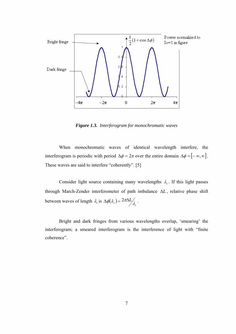
Figure 1.3. Interferogram for monochromatic waves
When monochromatic waves of identical wavelength interfere, the
interferogram is periodic with period πφ 2=∆ over the entire domain [ ]∞∞−=∆ ,φ .
These waves are said to interfere “coherently”. [5]
Consider light source containing many wavelengths iλ . If this light passes
through March-Zender interferometer of path imbalance L∆ , relative phase shift
between waves of length iλ is ( )i
iL
λπλφ ∆=∆ 2 .
Bright and dark fringes from various wavelengths overlap, ‘smearing’ the
interferogram; a smeared interferogram is the interference of light with “finite
coherence”.
7
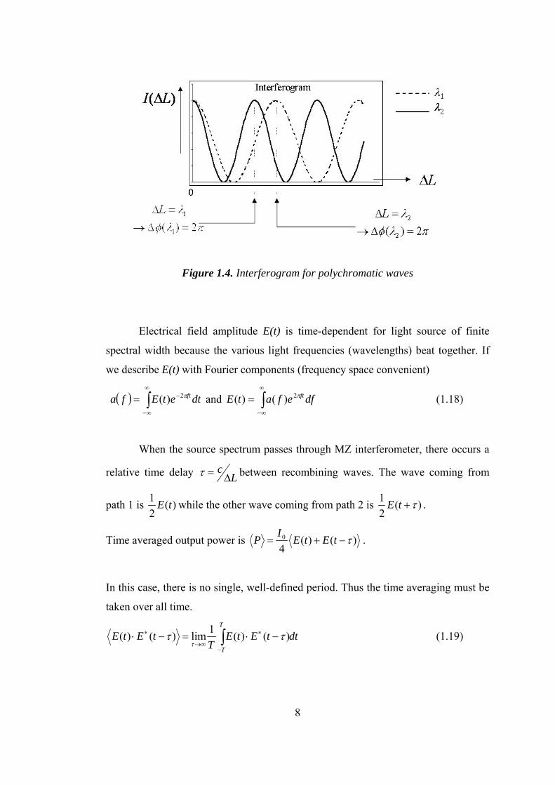
Figure 1.4. Interferogram for polychromatic waves
Electrical field amplitude E(t) is time-dependent for light source of finite
spectral width because the various light frequencies (wavelengths) beat together. If
we describe E(t) with Fourier components (frequency space convenient)
and (1.18) ( ) ∫∞
∞−
−= dtetEfa ftπ2)( ∫∞
∞−
= dfefatE ftπ2)()(
When the source spectrum passes through MZ interferometer, there occurs a
relative time delay Lc
∆=τ between recombining waves. The wave coming from
path 1 is )(21 tE while the other wave coming from path 2 is )(
21 τ+tE .
Time averaged output power is )()(40 τ−+= tEtEIP .
In this case, there is no single, well-defined period. Thus the time averaging must be
taken over all time.
dttEtET
tEtET
T∫
−
∗
∞→
∗ −⋅=−⋅ )()(1lim)()( τττ
(1.19)
8
The integral is the familiar autocorrelation function of )(τC ;
)()()( ττ −⋅= ∗ tEtEC .
Now the Wiener-Khintchine theorem relates the electric field autocorrelation
function )(τC and power spectrum ; )( fS
dteCfS iftπτ 2)()( −∞
∞−∫= and (1.20) ∫
∞
∞−
= dfefSC iftπτ 2)()(
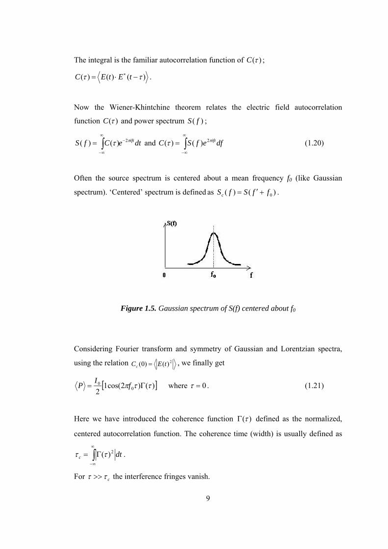
Often the source spectrum is centered about a mean frequency f0 (like Gaussian
spectrum). ‘Centered’ spectrum is defined as )()( 0ffSfSc +′= .
Figure 1.5. Gaussian spectrum of S(f) centered about f0
Considering Fourier transform and symmetry of Gaussian and Lorentzian spectra,
using the relation 2)()0( tECc = , we finally get
[ ])()2cos(12 00 ττπ Γ= fIP where 0=τ . (1.21)
Here we have introduced the coherence function )(τΓ defined as the normalized,
centered autocorrelation function. The coherence time (width) is usually defined as
∫∞
∞−
Γ= dtc2)(ττ .
For cττ >> the interference fringes vanish.
9
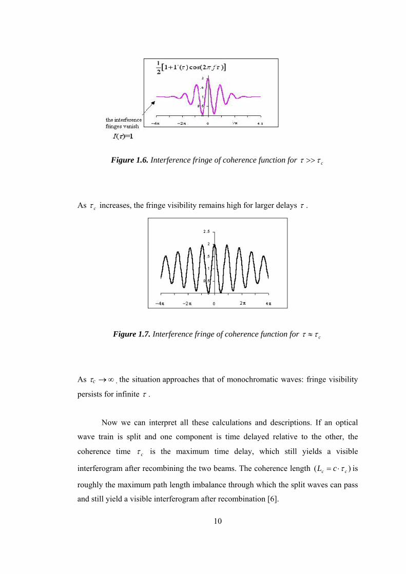
Figure 1.6. Interference fringe of coherence function for cττ >>
As cτ increases, the fringe visibility remains high for larger delays τ .
Figure 1.7. Interference fringe of coherence function for cττ ≈
As τc ∞→ , the situation approaches that of monochromatic waves: fringe visibility
persists for infinite τ .
Now we can interpret all these calculations and descriptions. If an optical
wave train is split and one component is time delayed relative to the other, the
coherence time cτ is the maximum time delay, which still yields a visible
interferogram after recombining the two beams. The coherence length )( cc cL τ⋅= is
roughly the maximum path length imbalance through which the split waves can pass
and still yield a visible interferogram after recombination [6].
10
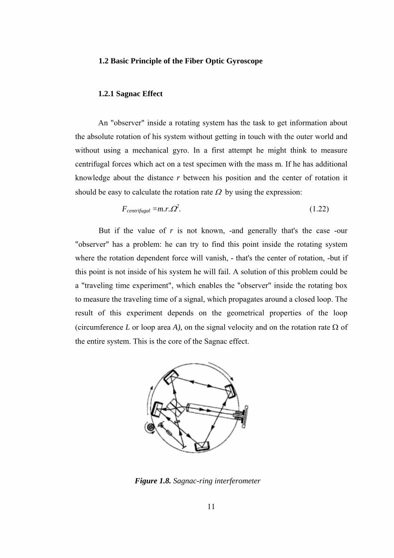
1.2 Basic Principle of the Fiber Optic Gyroscope
1.2.1 Sagnac Effect
An "observer" inside a rotating system has the task to get information about
the absolute rotation of his system without getting in touch with the outer world and
without using a mechanical gyro. In a first attempt he might think to measure
centrifugal forces which act on a test specimen with the mass m. If he has additional
knowledge about the distance r between his position and the center of rotation it
should be easy to calculate the rotation rate Ω by using the expression:
Fcentrifugal =m.r.Ω2. (1.22)
But if the value of r is not known, -and generally that's the case -our
"observer" has a problem: he can try to find this point inside the rotating system
where the rotation dependent force will vanish, - that's the center of rotation, -but if
this point is not inside of his system he will fail. A solution of this problem could be
a "traveling time experiment", which enables the "observer" inside the rotating box
to measure the traveling time of a signal, which propagates around a closed loop. The
result of this experiment depends on the geometrical properties of the loop
(circumference L or loop area A), on the signal velocity and on the rotation rate Ω of
the entire system. This is the core of the Sagnac effect.
Figure 1.8. Sagnac-ring interferometer
11
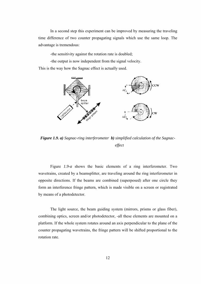
In a second step this experiment can be improved by measuring the traveling
time difference of two counter propagating signals which use the same loop. The
advantage is tremendous:
-the sensitivity against the rotation rate is doubled;
-the output is now independent from the signal velocity.
This is the way how the Sagnac effect is actually used.
Figure 1.9. a) Sagnac-ring interferometer b) simplified calculation of the Sagnac-
effect
Figure 1.9-a shows the basic elements of a ring interferometer. Two
wavetrains, created by a beamsplitter, are traveling around the ring interferometer in
opposite directions. If the beams are combined (superposed) after one circle they
form an interference fringe pattern, which is made visible on a screen or registrated
by means of a photodetector.
The light source, the beam guiding system (mirrors, prisms or glass fiber),
combining optics, screen and/or photodetector, -all these elements are mounted on a
platform. If the whole system rotates around an axis perpendicular to the plane of the
counter propagating wavetrains, the fringe pattern will be shifted proportional to the
rotation rate.
12
The actual effect is based on a traveling time -, or phase-difference between
the two wavetrains. This leads to a shift of the interference fringe pattern, and this
again can easily be detected [7].
A very simple calculation of the magnitude of this effect is based on circular
beam guiding configuration (Fig 2.2-b). The following parameters are used;
R Radius of the beam guiding system
L=2π.R Circumference of the beam guiding system
A=π.R2 Area of the beam guiding system
c light -/signal velocity
δ t= L / c = 2πR/c Traveling time of the wavetrains for one circle
Ω rotation rate of the beam guiding system
Light enters and exits the loop at a point fixed on the fiber. If the coil rotates,
the entry/ exit point rotates with fiber. There occurs a time difference for counter
propagating light waves to complete one loop.
c
tRt CW
CW)2( Ω−
=π
(1.23)
c
tRt CCW
CCW)2( Ω+
=π
(1.24)
Solving separately for and we find that to first order in RΩ/c, the
wave transit times differ by
CWt CCWt
⎟⎠⎞
⎜⎝⎛ Ω
=−=∆c
RcRttt CCWCW π4 . (1.25)
Usually the fiber is wrapped in a coil with N turns of radius R because this provides
adequate sensitivity. For N turns ∆t becomes;
⎟⎠⎞
⎜⎝⎛ Ω
=−=∆c
Rc
RNttt CCWCW π4 (1.26)
13

Substituting coil length RNL π2= and coil diameter D=2R,
2cLDt Ω
=∆ (1.27)
Phase shift;
2cDLt Ω⋅⋅⋅
=∆⋅=∆ωωφ , where ω is angular frequency of light wave (
vakumc λπω 2
= ).
Thus the Sagnac phase shift for light of wavelength λ in propagating through a coil
of length L and diameter D is;
cDL
S ⋅Ω⋅⋅⋅
=∆λ
πφ 2. (1.28)
The most important parameter for fiber optic gyroscopes is the gyro scale factor
(SF=∆ Sφ /Ω). [8]
cDLSF
⋅⋅⋅
=λ
π2. (1.29)
1.2.2 Bias Modulation
The fiber-optic gyroscope provides an interference signal of the Sagnac
effect, cDL
S ⋅Ω⋅⋅⋅
=∆λ
πφ 2 , with perfect contrast, since the phases as well as the
amplitudes of both counter propagating waves are perfectly equal at rest. The optical
power response is then a raised cosine function, )cos1(20
sIP φ∆+= , of the
rotation induces phase difference Sφ∆ , which is maximum at zero. To get high
sensitivity, this signal must be biased about an operating point with a nonzero
response slope:
([ ]bsI
P φφ ∆+∆+= cos120 ) , (1.30)
where bφ∆ is the phase bias. bφ∆ must be as stable as the anticipated sensitivity; that
is, significantly better than 1 µrad [6].
14
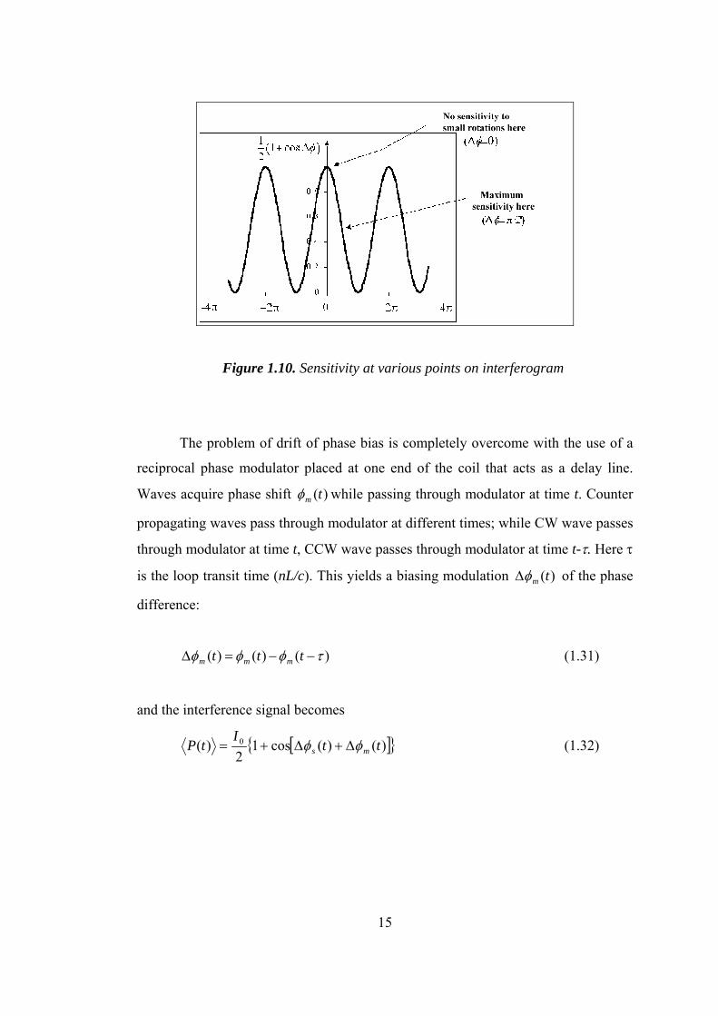
Figure 1.10. Sensitivity at various points on interferogram
The problem of drift of phase bias is completely overcome with the use of a
reciprocal phase modulator placed at one end of the coil that acts as a delay line.
Waves acquire phase shift )(tmφ while passing through modulator at time t. Counter
propagating waves pass through modulator at different times; while CW wave passes
through modulator at time t, CCW wave passes through modulator at time t-τ. Here τ
is the loop transit time (nL/c). This yields a biasing modulation )(tmφ∆ of the phase
difference:
)()()( τφφφ −−=∆ ttt mmm (1.31)
and the interference signal becomes
[ )()(cos12
)( 0 ttI
tP ms φφ ∆+∆+= ] (1.32)
15
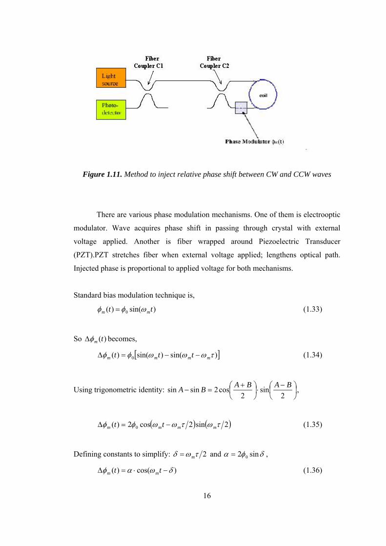
Figure 1.11. Method to inject relative phase shift between CW and CCW waves
There are various phase modulation mechanisms. One of them is electrooptic
modulator. Wave acquires phase shift in passing through crystal with external
voltage applied. Another is fiber wrapped around Piezoelectric Transducer
(PZT).PZT stretches fiber when external voltage applied; lengthens optical path.
Injected phase is proportional to applied voltage for both mechanisms.
Standard bias modulation technique is,
)sin()( 0 tt mm ωφφ = (1.33)
So )(tmφ∆ becomes,
[ )sin()sin()( 0 ]τωωωφφ mmmm ttt −−=∆ (1.34)
Using trigonometric identity: ⎟⎠⎞
⎜⎝⎛ −
⋅⎟⎠⎞
⎜⎝⎛ +
=−2
sin2
cos2sinsin BABABA ,
( ) ( )2sin2cos2)( 0 τωτωωφφ mmmm tt −=∆ (1.35)
Defining constants to simplify: 2τωδ m= and δφα sin2 0= ,
)cos()( δωαφ −⋅=∆ tt mm (1.36)
16
Now that the phase modulation term is known, returning to the detector signal
[ ] )(cos12
)( 0 tI
tP mS φφ ∆+∆+=
[ ] [ )(sin)sin()(cos)cos(120 tt
ImSmS φφφφ ∆∆−∆∆+= ]
[ ] [ )(sin)sin()cos(cos)(cos12
)( 0 δωαφδωαφ −⋅⋅∆−−⋅∆⋅+= tCostI
tP mSmS ]
(1.37)
The harmonic contents of this signal is to be found using Bessel function identities.
(1.38)
Here Jk( ) is kth Bessel function of the 1st kind.
From the Bessel identities above, it can be seen that
∗ [ )(sin tm ]φ∆ terms give odd harmonics of ωm
∗ [ )(cos tm ]φ∆ terms give odd harmonics of ωm
Frequency content of detector signal is
(1.39)
17
Signal at modulation frequency is
[ ]δωφαω
−⋅∆⋅−= tJItP mSm
cos)sin()()( 10 (1.40)
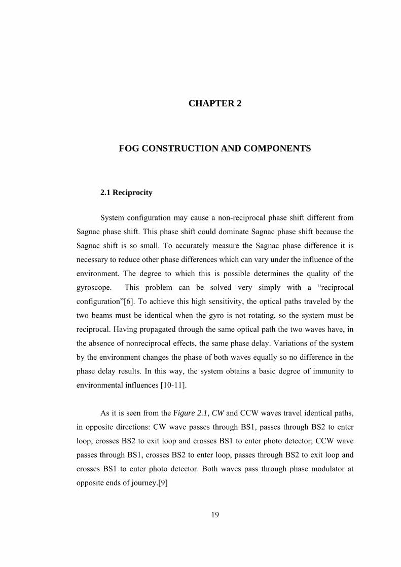
Detector signal contains all harmonics of ωm but desirable part is at 1st
harmonic of ωm. In order to extract signal at ωm only, Lock-in Amplifier (LIA) can
be used.
* If Sφ∆ =0, signal vanishes.
* For Sφ∆ << 1, signal ≈ SS φφ ∆≈∆sin
* Signal polarity reverses when rotation direction switches ( )SS φφ ∆−→∆ .
Comparing to unmodulated signal;
* Unmodulated signal ≈ ( φ∆+ cos1 ) ≈ ∆φ S 2 for Sφ∆ << 1.
* Sign of unmodulated signal independent of rotation direction.
Figure 1.12. Sinusoidal bias modulation: detector signal with finite Sagnac
phase shift [9]
18
CHAPTER 2
FOG CONSTRUCTION AND COMPONENTS
2.1 Reciprocity
System configuration may cause a non-reciprocal phase shift different from
Sagnac phase shift. This phase shift could dominate Sagnac phase shift because the
Sagnac shift is so small. To accurately measure the Sagnac phase difference it is
necessary to reduce other phase differences which can vary under the influence of the
environment. The degree to which this is possible determines the quality of the
gyroscope. This problem can be solved very simply with a “reciprocal
configuration”[6]. To achieve this high sensitivity, the optical paths traveled by the
two beams must be identical when the gyro is not rotating, so the system must be
reciprocal. Having propagated through the same optical path the two waves have, in
the absence of nonreciprocal effects, the same phase delay. Variations of the system
by the environment changes the phase of both waves equally so no difference in the
phase delay results. In this way, the system obtains a basic degree of immunity to
environmental influences [10-11].
As it is seen from the Figure 2.1, CW and CCW waves travel identical paths,
in opposite directions: CW wave passes through BS1, passes through BS2 to enter
loop, crosses BS2 to exit loop and crosses BS1 to enter photo detector; CCW wave
passes through BS1, crosses BS2 to enter loop, passes through BS2 to exit loop and
crosses BS1 to enter photo detector. Both waves pass through phase modulator at
opposite ends of journey.[9]
19
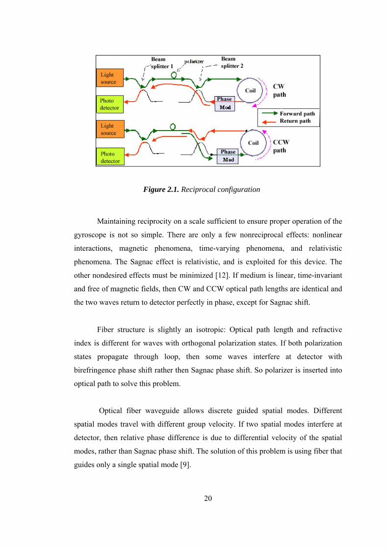
Figure 2.1. Reciprocal configuration
Maintaining reciprocity on a scale sufficient to ensure proper operation of the
gyroscope is not so simple. There are only a few nonreciprocal effects: nonlinear
interactions, magnetic phenomena, time-varying phenomena, and relativistic
phenomena. The Sagnac effect is relativistic, and is exploited for this device. The
other nondesired effects must be minimized [12]. If medium is linear, time-invariant
and free of magnetic fields, then CW and CCW optical path lengths are identical and
the two waves return to detector perfectly in phase, except for Sagnac shift.
Fiber structure is slightly an isotropic: Optical path length and refractive
index is different for waves with orthogonal polarization states. If both polarization
states propagate through loop, then some waves interfere at detector with
birefringence phase shift rather then Sagnac phase shift. So polarizer is inserted into
optical path to solve this problem.
Optical fiber waveguide allows discrete guided spatial modes. Different
spatial modes travel with different group velocity. If two spatial modes interfere at
detector, then relative phase difference is due to differential velocity of the spatial
modes, rather than Sagnac phase shift. The solution of this problem is using fiber that
guides only a single spatial mode [9].
20
2.2) Fiber Coil
Fiber coil is the most important part of Sagnac Interferometer, so does fiber
optic gyroscopes. Sagnac phase shift is proportional to product of coil length and
diameter. Mechanical and thermal characteristics of fiber coil are important for fiber
optic gyroscopes. Time-varying thermal or mechanical stress causes bias error. In
addition, gyro scale factor varies with coil dimension. In section 3.1, it is said that the
CW and CCW waves travel reciprocal paths if the fiber medium is time-invariant.
However, if fiber properties are time-varying, e.g., expanding/contracting fiber, CW
wave encounters variation at time t while CCW wave encounters variation at
different time, t-δt. Consequently a nonreciprocal phase shift exist, even if absence of
rotation which is a gyro error. It is obvious that, fiber characteristics are important
for fiber optic gyroscopes. The fiber used in fiber optic gyroscope must have some
characteristics. First, it must be single spatial mode because different modes have
different propagation velocities. Second, the fiber medium must be linear. If it is
nonlinear, Kerr effect error occurs. Third, fiber diameter must be large because
thermal phase noise worse for small fiber diameter and the last, loss in fiber must be
low because the ratio of signal to shot noise proportional to (detector power)1/2. As a
result, coils must be carefully wound to minimize thermal & stress gradients,
asymmetries, and dynamic responses. [9] (For detailed information see reference [6])
2.3) Light Source
There are few constraints on the source for a fiber optic gyroscope. Probably
the most obvious is that it must be able to inject a significant amount of optical
power, e.g., 100 µW or more, into a single-mode waveguide. Another restriction on
the source is set by noise due to Rayleigh backscattered light in the fiber. This has
been reduced primarily by reducing the coherence length of the source light. To
achieve current state-of-the-art short-term levels, it appears that the source coherence
must be less than, or approximately, 1 cm. Wavelength stability is another restriction
21
on the source because of the scale factor which is proportional to mean wavelength
[10].
Laser diode (LD) have high output power and coupling efficiency, but their
coherence is strong, and with a narrow optical spectrum width.
Light-emitting diodes (LED) have advantages of broad optical spectrum and
small coupling noises, but its output power and coupling efficiency are low.
Superluminescent diode (SLD) has high output power and a broad optical
spectrum width. It characterizes between LD and LED. It may suppress
nonreciprocal phase shift owing to Rayleigh scattering noise and nonlinearity Kerr
effect. SLD is an ideal light source for fiber optic gyroscope.
Advantages of SLD are being all-solid state, requiring low drive voltage,
having broad bandwidth (∆λ ∼ 20 nm at λ ∼ 850 nm) and short coherence length
(Lc ∼ 6 µm).
Disadvantage of SLD is having poor wavelength stability (400ppm/οC
temprature dependence and 40 ppm/mA drive current dependence) [13],[15].
Rare earth-doped fiber light source (FLS) is the other source used in fiber optic
gyroscope. To overcome the problem of SLD wavelength stability, FLS has been
developed. FLS has more complex configuration but this source is more useful than
SLD.
Advantages of FLS are having excellent wavelength stability possible, high
output power, unpolarized output that reduces polarization error, light generated
within SM fiber easily couples to fiber gyro and shapeable spectrum.
Disadvantage of FLS is having long coherence length (Lc ∼ 200 µm)
[14-16].
22
2.4) Coupler
Coupler functions in gyroscopes can be described as:
• Coupler 1 (“source” coupler)
o direct source light to gyro loop on forward path
o direct returning light to detector
• Coupler 2 (“coil” or “loop” coupler)
o Separate light into CW and CCW waves to traverse loop
o Recombine CW and CCW waves after loop [9]
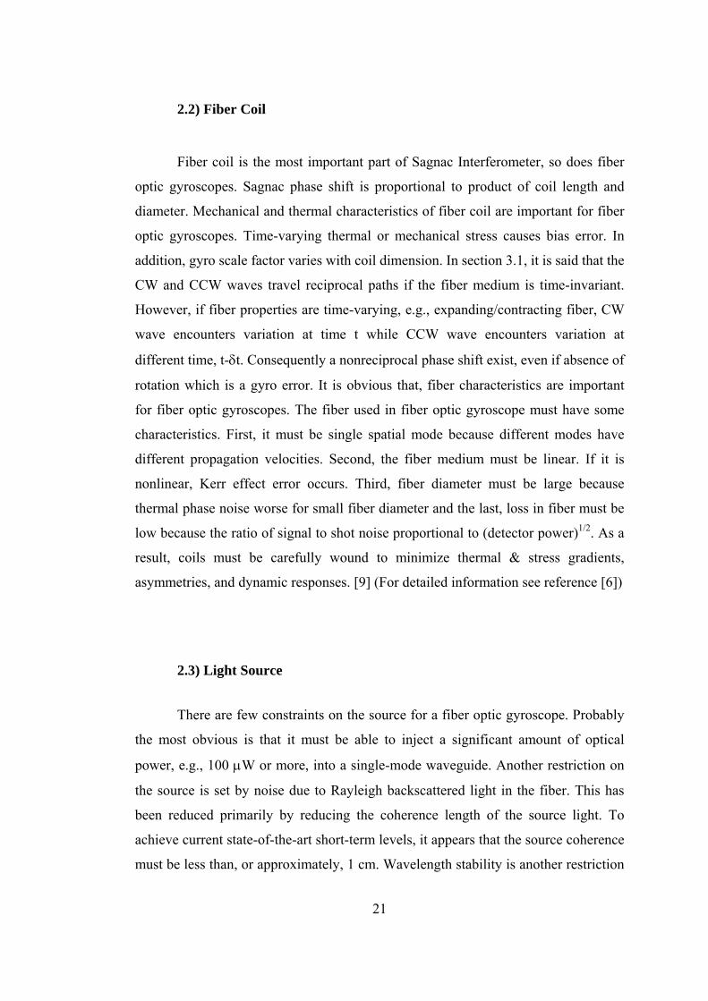
Consider perfectly matched interferometer with 50-50 splitter at entrance/exit.
Figure 2.2. Reciprocal use of coupler
At detector 1:
Both CW and CCW waves are transmitted once and reflected once. Beams are
traveled identical paths so 01 =∆φ .
ininininin ICosIIIIP =∆++= 11 44
244
φ
23
At detector 2:
Reflected wave has 90o phase shift relative to through wave so the phase shift
between CW and CCW waves is ∆φ2 = 180o. Therefore, the power detected here is
012 =−= inIPP . [6] This is true of cross-coupled and transmitted waves in a
coupler. Reciprocal configuration ensures both waves are transmitted/cross-coupled
equal number of times [9].
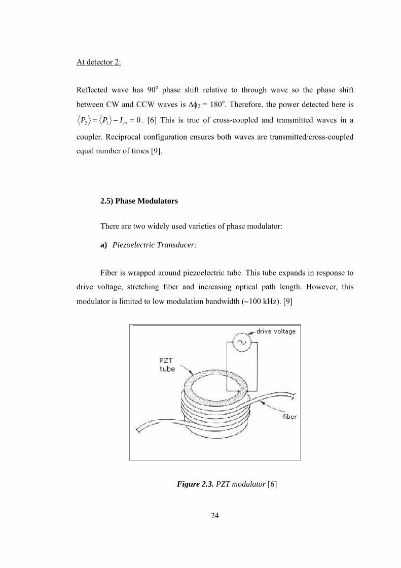
2.5) Phase Modulators
There are two widely used varieties of phase modulator:
a) Piezoelectric Transducer:
Fiber is wrapped around piezoelectric tube. This tube expands in response to
drive voltage, stretching fiber and increasing optical path length. However, this
modulator is limited to low modulation bandwidth (∼100 kHz). [9]
Figure 2.3. PZT modulator [6]
24
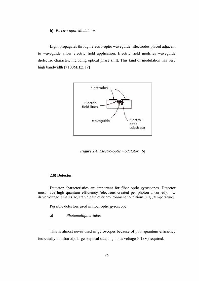
b) Electro-optic Modulator:
Light propagates through electro-optic waveguide. Electrodes placed adjacent
to waveguide allow electric field application. Electric field modifies waveguide
dielectric character, including optical phase shift. This kind of modulation has very
high bandwidth (>100MHz). [9]
Figure 2.4. Electro-optic modulator [6]
2.6) Detector
Detector characteristics are important for fiber optic gyroscopes. Detector must have high quantum efficiency (electrons created per photon absorbed), low drive voltage, small size, stable gain over environment conditions (e.g., temperature). Possible detectors used in fiber optic gyroscope:
a) Photomultiplier tube:
This is almost never used in gyroscopes because of poor quantum efficiency
(especially in infrared), large physical size, high bias voltage (∼1kV) required.
25
b) Avalanche photodiode:
This is seldom used in gyroscopes because of temperature-dependent gain,
non-optimum noise contribution and ∼100V bias voltage required.
c) PIN diode:
This is widely used in gyroscopes. Advantages of this detector are excellent
size and noise characteristics, good environmental stability and low cost [9].
26
CHAPTER 3
GYRO PERFORMANCE
Gyro performance depends on some conditions. These conditions are noise,
bias stability, input axis alignment, deadzone, scale factor.
3.1 Noise
The ideal performance of an optical gyroscope is limited by noise. The output
of the gyro is converted into an intensity variation that a detector measures. Any
chance in intensity due to noise can not be distinguished from a change in intensity
due to rotation. Therefore, the uncertainty in rotation rate is determined by the level
of noise in the system.
3.1.1 Shot Noise
Intensity changes due to source variation can be referenced out, but
fluctuations due to shot noise cannot be reduced, as they arise from a random
process. This is because of statistical fluctuations in photon flux at detector. The
uncertainty in the actual phase signal is given by
slope fringe
noiseshot photon =δφ . (3.1)
Plugging this into the sensitivity of a fiber gyro, the ultimate rotation uncertainty is
δφπλδRLc
4=Ω . [12] (3.2)
27
3.1.2 Johnson Noise
This occurs because of fluctuations in current across resistor due to thermal
motions of electrons within resistor.
3.1.3 Thermal Phase Noise
Thermal fluctuations occur in optical refractive index of fiber. This causes noise.
3.1.4 Relative Intensity Noise
This occurs because of beating of separate wavelengths within finite
bandwidth light spectrum[9] (For detailed information on noise see [12], [17], [18])
3.2. Bias Stability
When a gyro indicates finite rotation rate, even in the absence of true rotation
rate, the gyro is said to have a ‘bias offset’ or simply ‘bias’. Bias is not problematic if
it is stable. It can be calibrated and subtracted. However, mechanisms that produce
bias offset are generally not stable. Reciprocal gyro configuration makes
interferometer insensitive to environment but bias error mechanisms do not satisfy
reciprocity.
3.2.1 Bias Error Mechanisms
3.2.1.1. Modulator Error
Modulator error is produced by modulator. There are two kinds of modulator
error:
3.2.1.1.a) Nonlinearity
For an ideal modulator, optical phase shift strictly proportional to applied
voltage but for an imperfect modulation, optical phase shift responds nonlinearity to
28
voltage. This nonlinearity generates spurious second harmonic phase modulation and
creates spurious detector signal synchronous with phase modulation.
This problem can be eliminated by designing nearly perfect modulator, or
adjusting modulation frequency ωm at proper frequency ωp in order to vanish the
second harmonic term.
ωm = ωp = π/τ (3.3)
3.2.1.1.b) Intensity Modulation
Another modulator-induced bias error mechanism is intensity modulation.
Modulator applies time varying phase and attenuation to optical waves. Thus,
intensity modulation by the modulator produces a bias error which varies with
environment (e.g., temperature). This error also vanishes at proper frequency ωp.
3.2.1.2 Secondary waves
As it is said before, detector signal measures phase shift between ‘primary’
CW and CCW waves, which are forced to travel reciprocal paths. However other
‘secondary’ waves also propagate through gyroscope [see Clifford]. They do not
travel reciprocal paths. Backscattered waves and polarization cross-coupled waves
are two examples of these waves. These are sources of bias instability.
3.2.1.3 Nonreciprocal Effects
It is assumed that primary waves are reciprocal if they travel the same
physical path. This is not always true. Reciprocity is broken in some situations:
Shupe Effect:
If fiber properties vary with time, CW and CCW waves see fiber properties at
different time [22].
29
Kerr Effect:
If fiber properties are nonlinear, thus refractive index depends on electric
field amplitude; CW and CCW waves have different amplitudes [23].
Faraday Effect:
Magnetic field breaks CW-CCW symmetry.
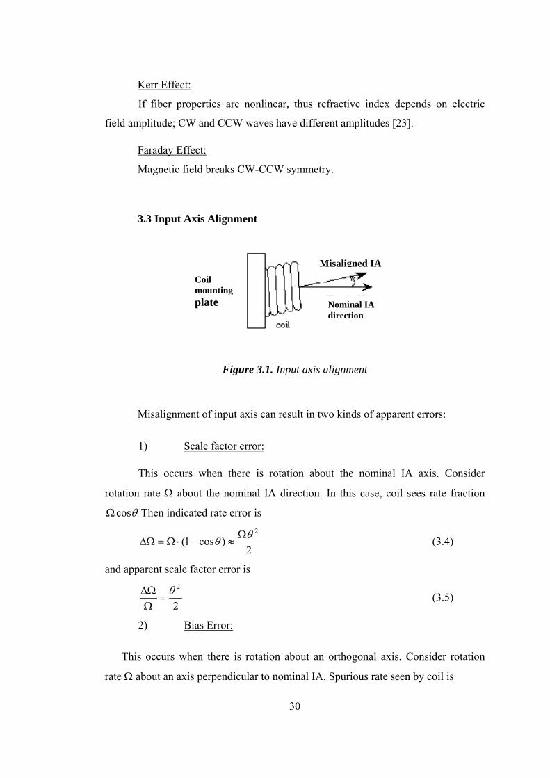
3.3 Input Axis Alignment
Misaligned IACoil mounting plate Nominal IA
direction
Figure 3.1. Input axis alignment
Misalignment of input axis can result in two kinds of apparent errors:
1) Scale factor error:
This occurs when there is rotation about the nominal IA axis. Consider
rotation rate Ω about the nominal IA direction. In this case, coil sees rate fraction
θcosΩ Then indicated rate error is
2)cos1(
2θθ Ω≈−⋅Ω=∆Ω (3.4)
and apparent scale factor error is
2
2θ=
Ω∆Ω (3.5)
2) Bias Error:
This occurs when there is rotation about an orthogonal axis. Consider rotation
rate Ω about an axis perpendicular to nominal IA. Spurious rate seen by coil is
30
θθ Ω≈⋅Ω=Ω sinerror (3.6)
this appears as bias error in absence of rotation about nominal IA axis.
Careful mechanical packaging is the solution to IA instability.
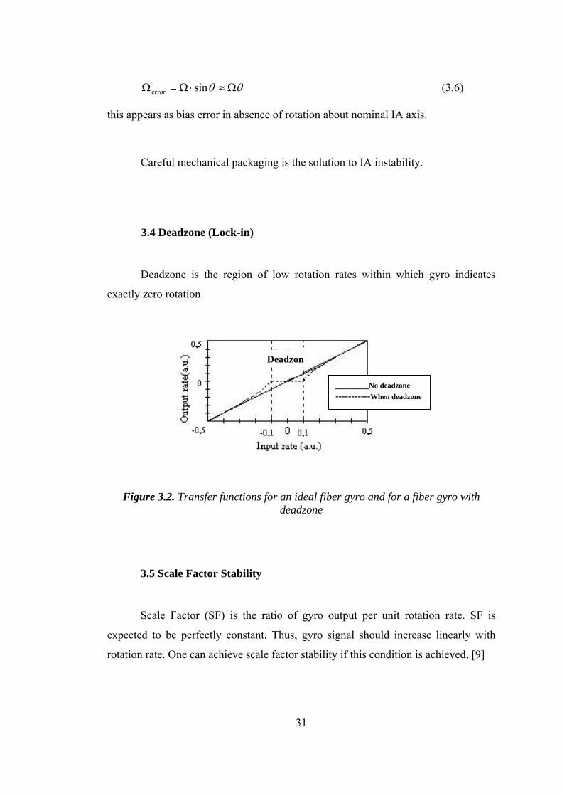
3.4 Deadzone (Lock-in)
Deadzone is the region of low rotation rates within which gyro indicates
exactly zero rotation.
Deadzon
_______No deadzone -----------When deadzone
Figure 3.2. Transfer functions for an ideal fiber gyro and for a fiber gyro with deadzone
3.5 Scale Factor Stability
Scale Factor (SF) is the ratio of gyro output per unit rotation rate. SF is
expected to be perfectly constant. Thus, gyro signal should increase linearly with
rotation rate. One can achieve scale factor stability if this condition is achieved. [9]
31
CHAPTER 4
SIMULATION ON
INTERFEROMETRIC FIBER OPTIC GYROSCOPE
WITH AMPLIFIED OPTICAL FEEDBACK (FE_FOG)
4.1 Properties of the Simulation Program, VPItransmissionMakerTM
Simulation Program VPItransmissionMaker enables the user to prepare and
configure photonic simulations on her/his computer. VPItransmissionMaker can fully
verify link designs at a sampled-signal level to identify further cost savings,
investigate novel technologies, or fulfill specialist requirements. Links can be
automatically imported from VPIlinkConfigurator for detailed design and
optimization. VPItransmissionMaker is widely used as an R&D tool to evaluate
novel component and subsystems designs in a systems context, investigate and
optimize systems technologies (e.g. coding, modulation, monitoring, compensation,
regeneration). VPIcomponentMaker™ allows active and passive devices, and optical
amplifiers to be designed, and their performance abstracted for systems-level
simulations with VPItransmissionMaker™. New amplifier technologies (multistage,
multipump, hybrid and waveguide) can be developed, optical signal processing
(wavelength conversion, clock recovery, partial regeneration) investigated, and the
performance of lasers and tunable lasers in conjunction with integrated modulators
can be assessed [21].
32
Sophisticated design tool for photonic devices, components, systems and
network are developed. Tools must support signal representations and algorithms for
modeling optical components and network elements at different level of
abstraction.[20]
4.2 Signal Representations
Data exchange can be organized in blocks or by transmitting individual samples.
The Block Mode is more suitable for systems simulations where components are
widely-spaced compared with the modeled time, or where signals flow
unidirectionally, from transmitter to receiver. This is the most efficient form of
simulation, as modules are only ‘fired’ when data passes through them. Passing data between modules on a sample-by-sample basis is necessary
when delay between the modules is much shorter than a block length: the modules
must communicate rapidly in order to fully simulate their joint behavior. A good
example of an application of Sample Mode is the stabilization of lasers using
external cavities. The cavity and laser have to be simulated simultaneously (and fire
at each iteration) in order to determine the optical spectrum of the compound cavity
and its modulation dynamics. Because of bidirectional signal flow and delay between the modules is
important in fiber-optic gyros, Sample Mode signal representation must be used in
the simulation. [20]
4.3 Global Variables
The default Global Variables are:
TimeWindow: This sets the duration of the blocks in seconds. For simulations the
TimeWindow must be set so the block contains 2m, (m integer) data bits. This is
achieved by setting
TimeWindow = 2m / BitRateDefault
33
Because VPltransmissionMaker parameters can be expressions, a valid input is
therefore
TimeWindow = 128.0 / 2.5e9 for 128-bits at 2.5 Gbit/s.
A long time window leads to greater simulation accuracy (e.g. in BER estimation, or
in spectral resolution), but increases computation time.
BoundaryConditions:
This parameter sets whether the data within a block is considered to be
periodic or aperiodic. If it is periodic, then all frequency components are considered
to be exact harmonics of 1/TimeWindow. It has several advantages when modeling
dispersive nonlinear optical fibers. If the Boundary Conditions are aperiodic, the
data in successive blocks is 'stitched1 together. This is useful for modeling
components with long time constants compared with the bit-rate, such as
semiconductor lasers, because visualizers are updated every block, but the
simulation and the laser dynamics extend over several blocks. Using aperiodic
boundary conditions requires the aperiodic fiber model.
SampleRateDefault:
The modules where the parameter
SampleRate = SampleRateDefault
will use the value of SampleRateDefault which is given a value in the Global Variables.
This is a useful technique when all transmitters are using the same sample rate, as the
sample rate can be set with the single global variable. For digital simulations, the sample
rate of each module must be a power of two multiple of the BitRate. That is:
SampleRate = 2m. BitRate (where m is an integer)
Because the Parameter Editor accepts expressions, this can be entered easily, for
example SampleRate = 16∗2.5e9, gives an optical bandwidth of 16 times 2.5Gbit/s [20].
34
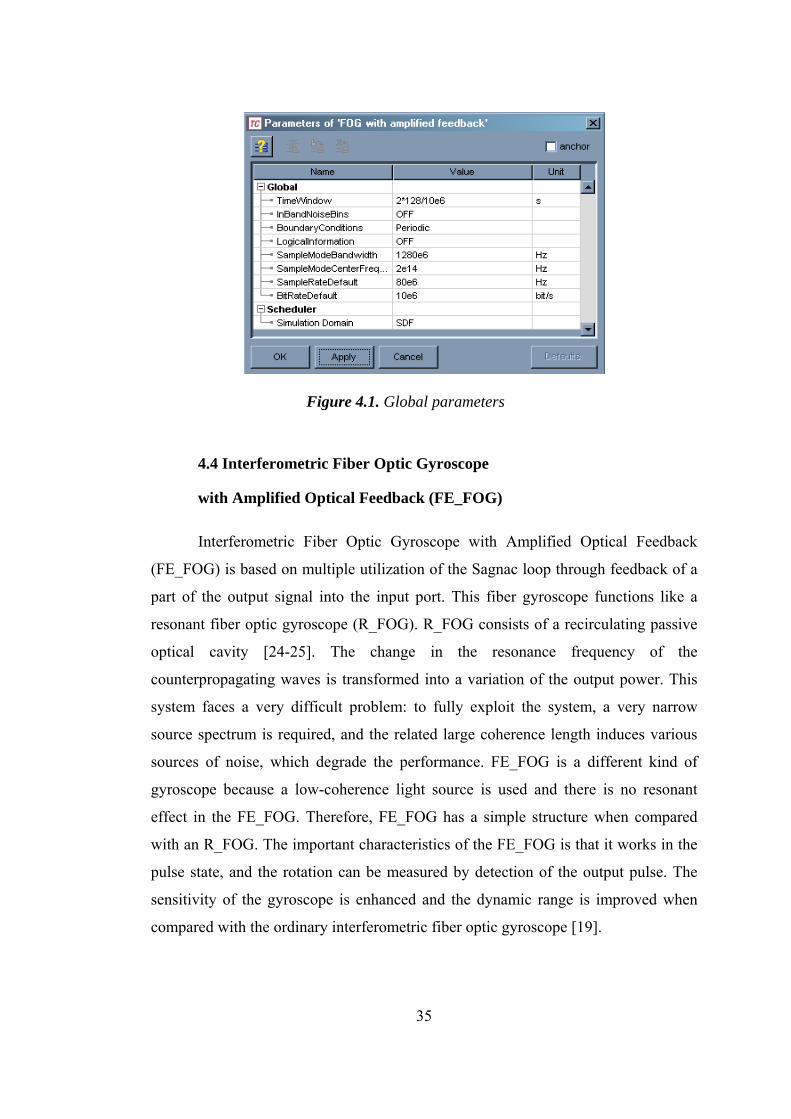
Figure 4.1. Global parameters
4.4 Interferometric Fiber Optic Gyroscope
with Amplified Optical Feedback (FE_FOG)
Interferometric Fiber Optic Gyroscope with Amplified Optical Feedback
(FE_FOG) is based on multiple utilization of the Sagnac loop through feedback of a
part of the output signal into the input port. This fiber gyroscope functions like a
resonant fiber optic gyroscope (R_FOG). R_FOG consists of a recirculating passive
optical cavity [24-25]. The change in the resonance frequency of the
counterpropagating waves is transformed into a variation of the output power. This
system faces a very difficult problem: to fully exploit the system, a very narrow
source spectrum is required, and the related large coherence length induces various
sources of noise, which degrade the performance. FE_FOG is a different kind of
gyroscope because a low-coherence light source is used and there is no resonant
effect in the FE_FOG. Therefore, FE_FOG has a simple structure when compared
with an R_FOG. The important characteristics of the FE_FOG is that it works in the
pulse state, and the rotation can be measured by detection of the output pulse. The
sensitivity of the gyroscope is enhanced and the dynamic range is improved when
compared with the ordinary interferometric fiber optic gyroscope [19].
35
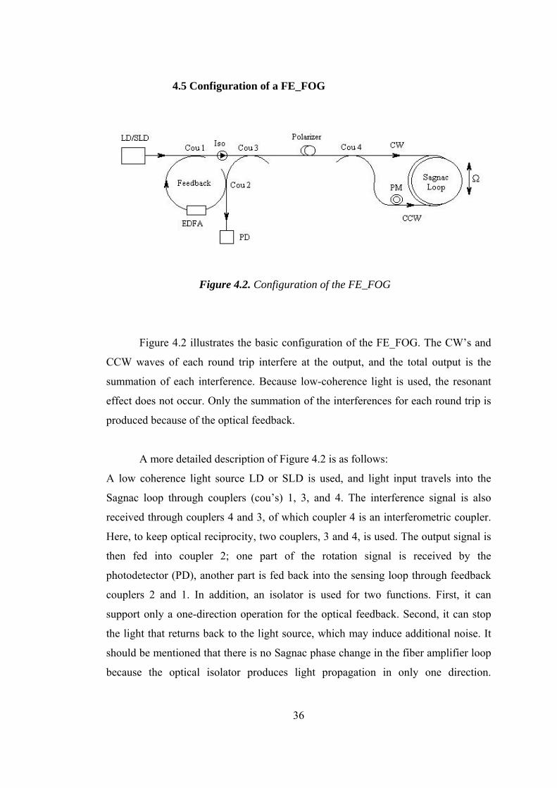
4.5 Configuration of a FE_FOG
Figure 4.2. Configuration of the FE_FOG
Figure 4.2 illustrates the basic configuration of the FE_FOG. The CW’s and
CCW waves of each round trip interfere at the output, and the total output is the
summation of each interference. Because low-coherence light is used, the resonant
effect does not occur. Only the summation of the interferences for each round trip is
produced because of the optical feedback.
A more detailed description of Figure 4.2 is as follows:
A low coherence light source LD or SLD is used, and light input travels into the
Sagnac loop through couplers (cou’s) 1, 3, and 4. The interference signal is also
received through couplers 4 and 3, of which coupler 4 is an interferometric coupler.
Here, to keep optical reciprocity, two couplers, 3 and 4, is used. The output signal is
then fed into coupler 2; one part of the rotation signal is received by the
photodetector (PD), another part is fed back into the sensing loop through feedback
couplers 2 and 1. In addition, an isolator is used for two functions. First, it can
support only a one-direction operation for the optical feedback. Second, it can stop
the light that returns back to the light source, which may induce additional noise. It
should be mentioned that there is no Sagnac phase change in the fiber amplifier loop
because the optical isolator produces light propagation in only one direction.
36
In this system, the weak feedback signal is amplified by a fiber amplifier (EDFA).
However, the gain of EDFA must be adjusted properly so that there is no laser
emission. In addition, it is assumed that the fiber amplifier is operating in a linear
mode so there are no power-level effects.
The total output signal is a summation of the interference of CW and CCW
waves for each round trip. Because a phase modulator is placed within the Sagnac
loop, the total output signal is a series of short pulses if the frequency of phase
modulator is selected properly. To realize pulse operation, modulation frequency of
the phase modulator and round-trip-time delay must be selected to satisfy a relation
of πτω nm 2= where ωm is the angular frequency of the phase modulation and τ is
the time delay of the light through the whole round trip, which includes the Sagnac-
loop plus the fiber-amplifier delay. If there is deterioration in the pulse shape as the
modulation becomes detuned, it can be more or less compensated by a variation of
the EDFA gain. The sharpness of the output pulse can be obtained by an adjustment
of the feedback couplers and the fiber amplifier. In addition, it should be noted that
the gain of EDFA is a function of the wavelength. Therefore, the wavelength stability
of the low-coherence light source is expected. Indeed, the wavelength stability of the
light source is the key issue for the scalar factor in any fiber optic gyroscope [19].
4.6 Theory
The first time interference signal without feedback has the same form as in that in
the ordinary interferometric fiber optic gyroscope, which is expressed as
( ) ( )[ tKtP mes ]ωφφν coscos111 ++= , (4.1)
where ν is the interferometric coefficient, which is a parameter of fringe contrast,
and K1 is a parameter that express the loss resulting from the Sagnac interferometer,
37
ωm is the modulation frequency (ωm = 2πƒm), φe is the effective phase modulation
depth, which is expressed as
)sin(2 smme f τπφφ = , (4.2)
τs is the wave propagation time through the Sagnac loop and expressed as τs=nL/c
where L is the length of the loop, and φm is the phase-modulation depth. φs is the
Sagnac phase shift induced by rotational movement, which is expressed as
cRL
s0
4λ
πφ Ω= . (4.3)
Here Ω is the rotation rate, R is the radius of the Sagnac loop, and c is the velocity of
light propagation in free space.
Considering the effect of optical feedback, the second-time interference signal
experienced after the feedback has been derived is
( ) [ ] [ ]( ) ttKAKtP mesmmes ωφφντωωφφν coscos1)cos(cos1212 ++×−++= (4.4)
and the third-time interference signal that occurs after feedback has been twice
derived is
( ) [ ]
[ ]
( )[ ] t
t
tKKAtP
mes
mmes
mmes
ωφφν
τωωφφν
τωωφφν
coscos1
)cos(cos1
)2cos(cos1)( 222
31
23
++×
−++×
−++=
(4.5)
where A is the gain of the fiber amplifier and K2 is a parameter that depends on the
coupling ratio of the feedback couplers and the transmission loss in the feedback
loop. For simplicity, it is assumed that K′ =K1K2. The total output at the
38
photodetector is the summation of the number of above-mentioned interferences and
is expressed as
Κ+++= )()()()( 321 tPtPtPtPtotal . (4.6)
If πτω nm 2= , the total photodetector output can be realized by proper adjustment of
the modulation frequency to match the round-trip time, and is )(tPtotal
( )[ ] ( )[ ]tKAtK
tPmes
mestotal ωφφν
ωφφνcoscos11
coscos1)(
++′−++
= , (4.7)
where K is the photodetecting coefficient.
Because the total output is a series of short pulses, the peak value can be
determined through the following equation:
0)( =′ tPtotal . (4.8)
Thus,
( )[ ]0cossin =+ tK mes ωφφν , (4.9)
and
( )[ ] πωφφ ntmes 2cos =+ , n=0,1,2,… (4.10)
This is the condition required to find the peak position of the output pulse that is
valid for both cases of rotation and nonrotation. From this equation and condition it
can be seen that the output pulse shifts if rotation occurs. This characteristic can be
utilized for the rotation measurement [19].
39
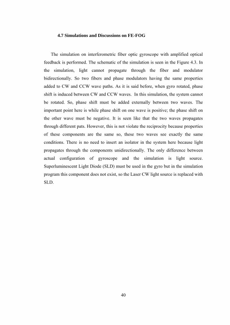
4.7 Simulations and Discussions on FE-FOG
The simulation on interferometric fiber optic gyroscope with amplified optical
feedback is performed. The schematic of the simulation is seen in the Figure 4.3. In
the simulation, light cannot propagate through the fiber and modulator
bidirectionally. So two fibers and phase modulators having the same properties
added to CW and CCW wave paths. As it is said before, when gyro rotated, phase
shift is induced between CW and CCW waves. In this simulation, the system cannot
be rotated. So, phase shift must be added externally between two waves. The
important point here is while phase shift on one wave is positive; the phase shift on
the other wave must be negative. It is seen like that the two waves propagates
through different pats. However, this is not violate the reciprocity because properties
of these components are the same so, these two waves see exactly the same
conditions. There is no need to insert an isolator in the system here because light
propagates through the components unidirectionally. The only difference between
actual configuration of gyroscope and the simulation is light source.
Superluminescent Light Diode (SLD) must be used in the gyro but in the simulation
program this component does not exist, so the Laser CW light source is replaced with
SLD.
40
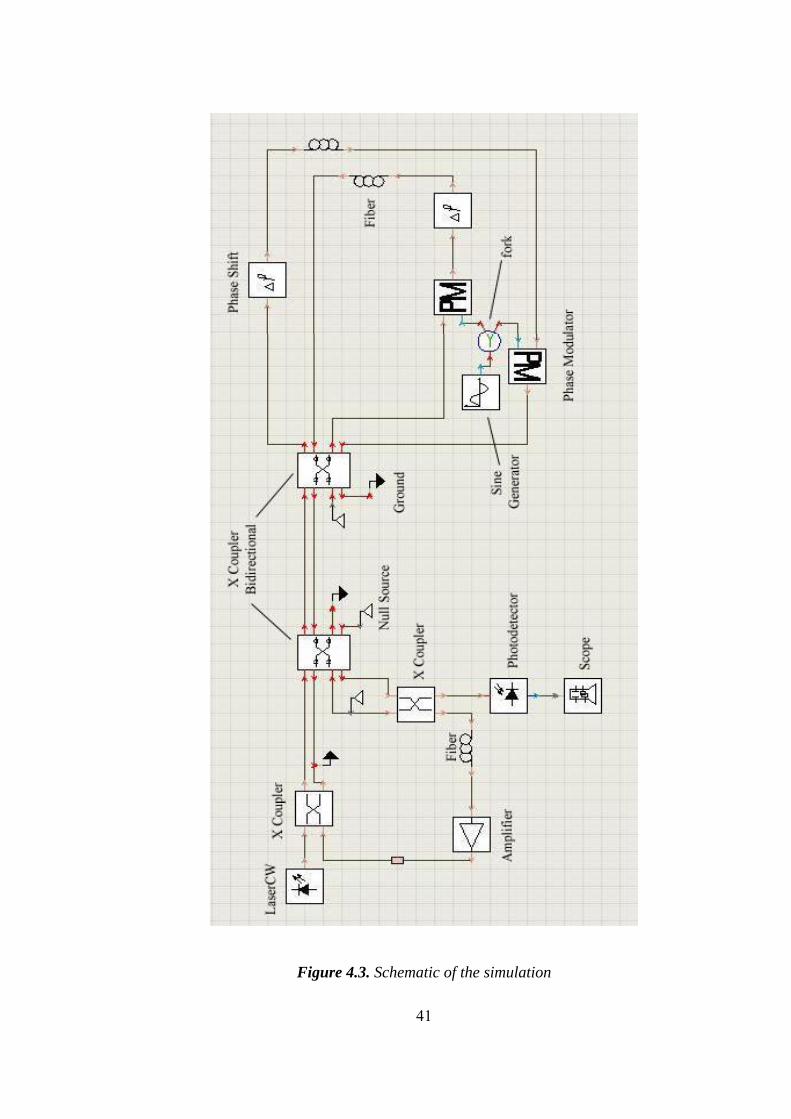
Figure 4.3. Schematic of the simulation
41
4.8 Modules Used in the Schematic*
4.8.1 LaserCW
LaserCW is used as a light source in the schematic. The module produces a
continuous wave (CW) optical signal. The parameters of the module are shown in the
Figure 4.4.
Figure 4.4. Parameters of LaserCW
* For detailed information see Appendix A.
42
4.8.2 X Coupler and X Coupler Bidirectional
X Coupler models an optical coupler for combining or splitting of optical
signals. X Coupler Bidirectional acts as a bidirectional X Coupler.
In simulation CoupleFactor default parameter 0,5 is used for both couplers.
4.8.3 Phase Shift
The module adds a time-independent phase advance to the optical input
signal. This module is used for simulating the Sagnac phase shift.
The parameter PhaseShift has changed several times and we got the solutions
for each value.
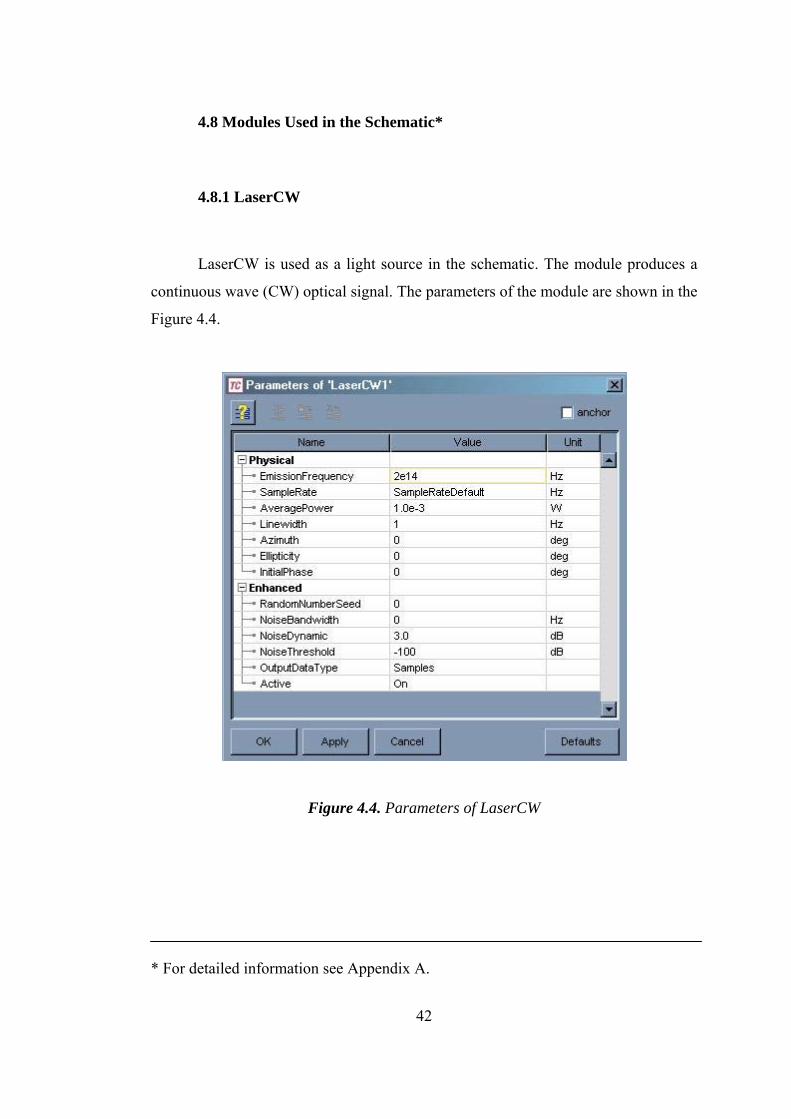
4.8.4 Sine Generator (Electrical)
This module is used for bias modulation It generates an electrical sine
waveform superimposed on a constant bias..
The parameters of the module are illustrated in Figure 4.5.
Figure 4.5. Parameters of Sine Generator
43
4.8.5 Multiple Output Connector (Fork)
This module copies input particles to each output.
4.8.6 Modulator Phase
Phase modulator is also used for bias modulation. The module simulates an
ideal phase modulator (PM).
The only parameter PhaseDeviation for PM was taken 180 deg.
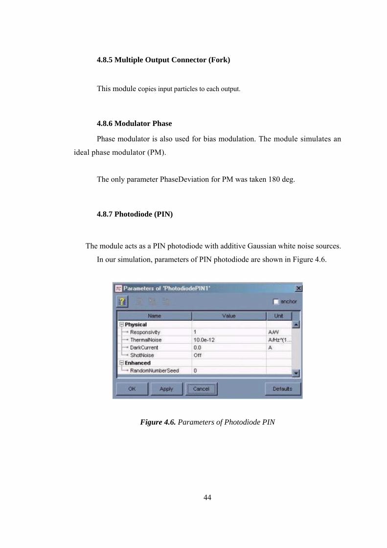
4.8.7 Photodiode (PIN)
The module acts as a PIN photodiode with additive Gaussian white noise sources.
In our simulation, parameters of PIN photodiode are shown in Figure 4.6.
Figure 4.6. Parameters of Photodiode PIN
44
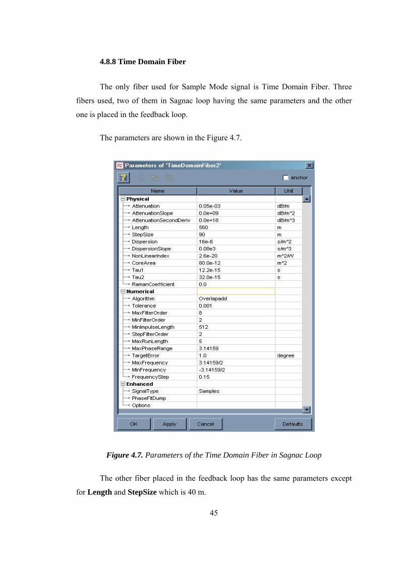
4.8.8 Time Domain Fiber
The only fiber used for Sample Mode signal is Time Domain Fiber. Three
fibers used, two of them in Sagnac loop having the same parameters and the other
one is placed in the feedback loop.
The parameters are shown in the Figure 4.7.
Figure 4.7. Parameters of the Time Domain Fiber in Sagnac Loop
The other fiber placed in the feedback loop has the same parameters except
for Length and StepSize which is 40 m.
45
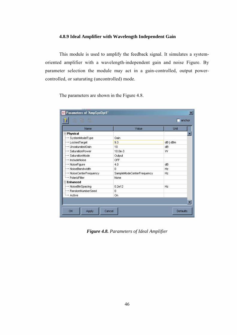
4.8.9 Ideal Amplifier with Wavelength Independent Gain
This module is used to amplify the feedback signal. It simulates a system-
oriented amplifier with a wavelength-independent gain and noise Figure. By
parameter selection the module may act in a gain-controlled, output power-
controlled, or saturating (uncontrolled) mode.
The parameters are shown in the Figure 4.8.
Figure 4.8. Parameters of Ideal Amplifier
46
4.9 Results
In the simulation, the total output wave is the summation of each interference
signal. Recall the equations (4.7), (4.10).
( )[ ] ( )[ ]tKAtK
tPmes
mestotal ωφφν
ωφφνcoscos11
coscos1)(
++′−++
= , and (4.7)
( )[ ] πωφφ ntmes 2cos =+ , n=0, 1, 2,… (4.10)
As it is said before, in order to achieve sharp pulses, frequency of the phase
modulator must be selected properly: πτω nm 2= (τ: total round trip time). In the
simulation, Sagnac loop delay τs is 1,8 µs and feedback delay is 0,3 µs. So τ = 2,1 µs
and ƒm = ωm / 2π = 4.76.105 Hz.
First, the simulation is run for nonrotation case (φs = 0). This means that
phase shifters are set to zero. Here, equation 4.10 is satisfied only when n = 0. In this
case, the peak positions of the output pulse are determined by
πω2
120
+=
itm , i = 0,1,2,… (4.11)
Here t0 represents the peak positions corresponding to the nonrotation case and i
denotes the peak number of the output pulse in the time axis. Peak positions are not
affected by the phase modulation depth φe when there is no rotation. Figure 4.9
shows the output of the simulation when φs = 0, φe = 1.24 π rad.
47
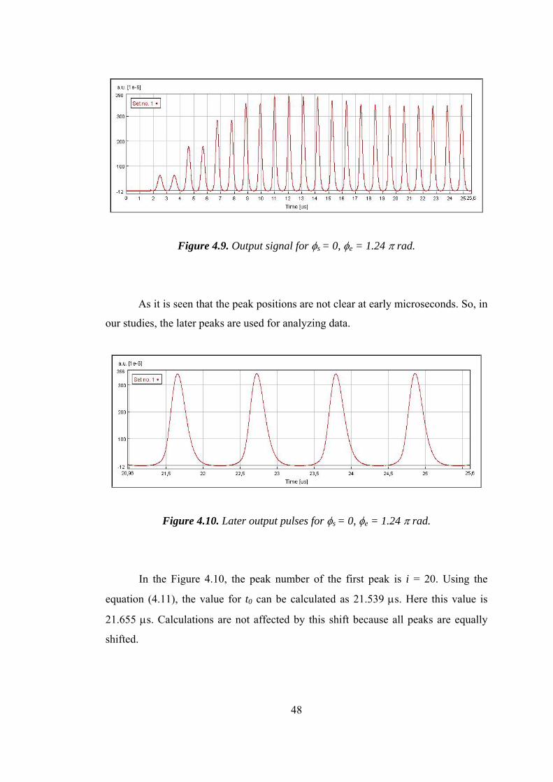
Figure 4.9. Output signal for φs = 0, φe = 1.24 π rad.
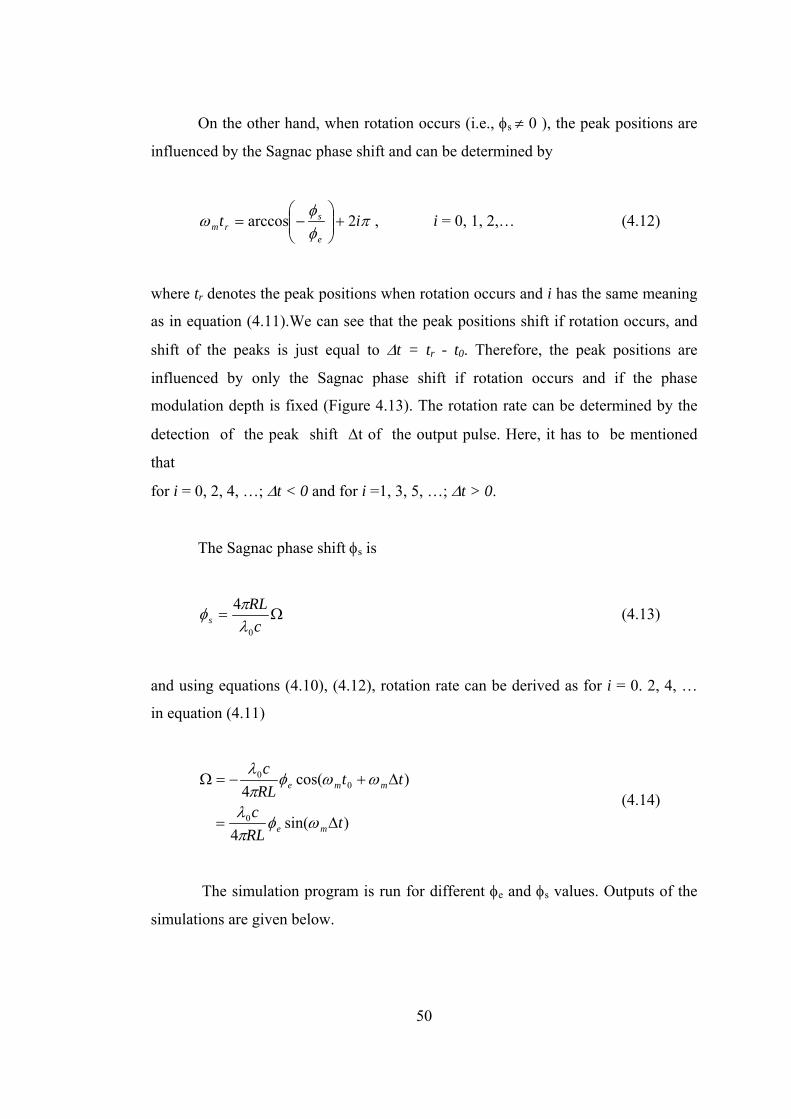
As it is seen that the peak positions are not clear at early microseconds. So, in
our studies, the later peaks are used for analyzing data.
Figure 4.10. Later output pulses for φs = 0, φe = 1.24 π rad.
In the Figure 4.10, the peak number of the first peak is i = 20. Using the
equation (4.11), the value for t0 can be calculated as 21.539 µs. Here this value is
21.655 µs. Calculations are not affected by this shift because all peaks are equally
shifted.
48

Figure 4.11 shows the output of the simulation when φs = 0, φe = 1.85 π rad.
When Figure 4.9 and figure 4.11 are compared, the relation between φe and sharpness
is obviously seen.
Figure 4.11. Output signal for φs = 0, φe = 1.85 π rad.
The shape of the pulse depends on two variables: gain of the amplifier and
modulation depth φe. The sharpness of the pulse can be adjusted by both the gain and
φe. If the gain is increased, the pulse can be sharpened.
Figure 4.12. Comparison between two gain values (a) 8 dB and (b) 9.3 dB
for φe = 1.24 π rad.
49
On the other hand, when rotation occurs (i.e., φs ≠ 0 ), the peak positions are
influenced by the Sagnac phase shift and can be determined by
πφφ
ω ite
srm 2arccos +⎟⎟
⎠
⎞⎜⎜⎝
⎛−= , i = 0, 1, 2,… (4.12)
where tr denotes the peak positions when rotation occurs and i has the same meaning
as in equation (4.11).We can see that the peak positions shift if rotation occurs, and
shift of the peaks is just equal to ∆t = tr - t0. Therefore, the peak positions are
influenced by only the Sagnac phase shift if rotation occurs and if the phase
modulation depth is fixed (Figure 4.13). The rotation rate can be determined by the
detection of the peak shift ∆t of the output pulse. Here, it has to be mentioned
that
for i = 0, 2, 4, …; ∆t < 0 and for i =1, 3, 5, …; ∆t > 0.
The Sagnac phase shift φs is
Ω=c
RLs
0
4λπφ (4.13)
and using equations (4.10), (4.12), rotation rate can be derived as for i = 0. 2, 4, …
in equation (4.11)
)sin(4
)cos(40
00
tRLc
ttRLc
me
mme
∆=
∆+−=Ω
ωφπλ
ωωφπλ
(4.14)
The simulation program is run for different φe and φs values. Outputs of the
simulations are given below.
50
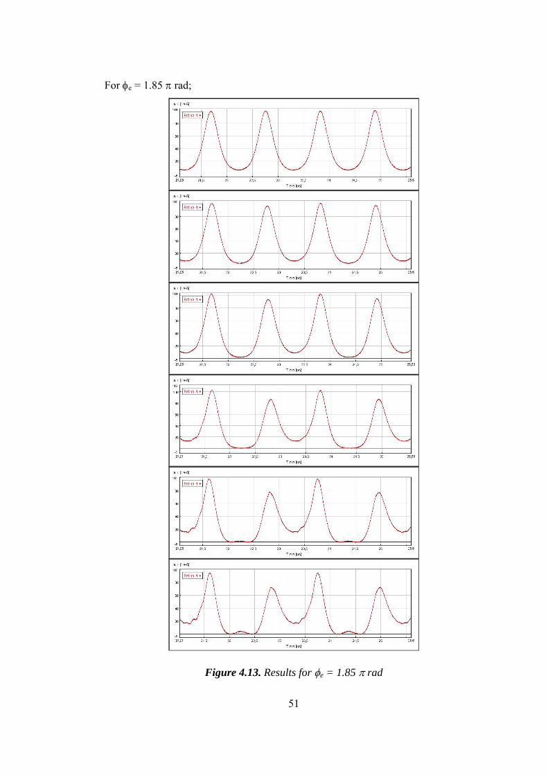
For φe = 1.85 π rad;
Figure 4.13. Results for φe = 1.85 π rad
51
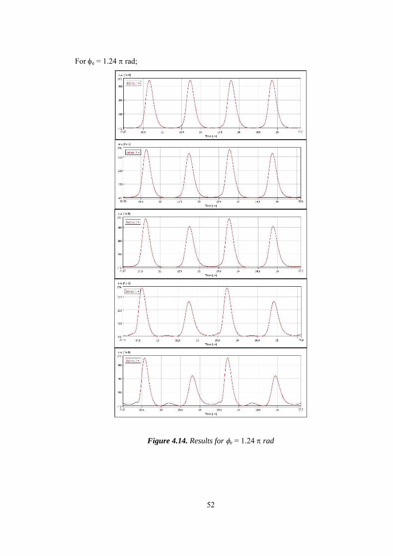
For φe = 1.24 π rad;
Figure 4.14. Results for φe = 1.24 π rad
52
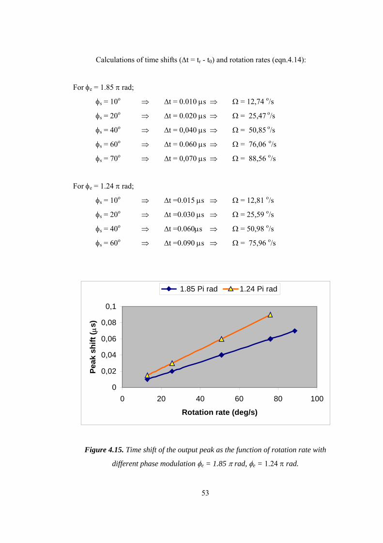
Calculations of time shifts (∆t = tr - t0) and rotation rates (eqn.4.14):
For φe = 1.85 π rad;
φs = 10o ⇒ ∆t = 0.010 µs ⇒ Ω = 12,74 o/s
φs = 20o ⇒ ∆t = 0.020 µs ⇒ Ω = 25,47 o/s
φs = 40o ⇒ ∆t = 0,040 µs ⇒ Ω = 50,85 o/s
φs = 60o ⇒ ∆t = 0.060 µs ⇒ Ω = 76,06 o/s
φs = 70o ⇒ ∆t = 0,070 µs ⇒ Ω = 88,56 o/s
For φe = 1.24 π rad;
φs = 10o ⇒ ∆t =0.015 µs ⇒ Ω = 12,81 o/s
φs = 20o ⇒ ∆t =0.030 µs ⇒ Ω = 25,59 o/s
φs = 40o ⇒ ∆t =0.060µs ⇒ Ω = 50,98 o/s
φs = 60o ⇒ ∆t =0.090 µs ⇒ Ω = 75,96 o/s
0
0,02
0,04
0,06
0,08
0,1
0 20 40 60 80 10
Rotation rate (deg/s)
Peak
shi
ft ( µ
s)
0
1.85 Pi rad 1.24 Pi rad
Figure 4.15. Time shift of the output peak as the function of rotation rate with
different phase modulation φe = 1.85 π rad, φe = 1.24 π rad.
53
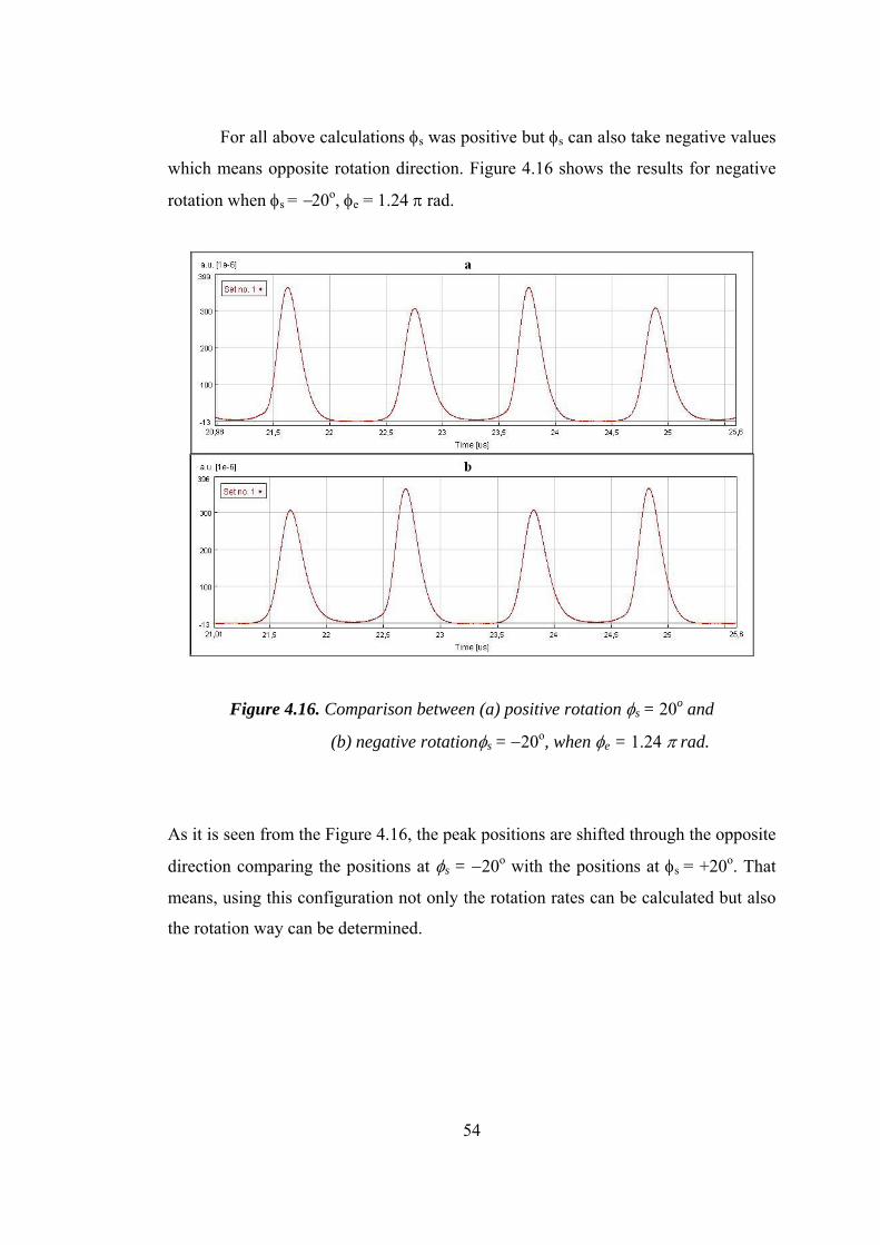
For all above calculations φs was positive but φs can also take negative values
which means opposite rotation direction. Figure 4.16 shows the results for negative
rotation when φs = −20o, φe = 1.24 π rad.
Figure 4.16. Comparison between (a) positive rotation φs = 20o and
(b) negative rotationφs = −20o, when φe = 1.24 π rad.
As it is seen from the Figure 4.16, the peak positions are shifted through the opposite
direction comparing the positions at φs = −20o with the positions at φs = +20o. That
means, using this configuration not only the rotation rates can be calculated but also
the rotation way can be determined.
54
CHAPTER 5
CONCLUSION
In this work, a novel interferometric fiber optic gyroscope that is based on
multiple utilizations of the Sagnac loop by amplified optical feedback (FE_FOG) has
been proposed and simulated. A software, VPItransmissionMakerTM, developed by
VPIsystems, was used.
In FE_FOG, low coherence light sources (SLD) are used. There is no such
kind of source in VPItransmissionMakerTM so a laser continuous wave (LaserCW)
was used in simulation. Amplification of a weak feedback gyroscope signal was
performed by EDFA.
The output of this gyroscope is in pulse state if the modulation frequency of
the phase modulator matches the total round trip. The round-trip time was calculated
and proper modulation frequency was selected.
The resolution of the rotation measurement depends on the sharpness of the
output pulse. The sharpness of the output pulse was adjusted with the gain of
amplifier and the phase modulation depth. It is seen that, increasing the gain of the
amplifier improves the sharpness of the output pulse.
The positions of the output pulses, which is important to measure the rotation
rate, were determined for several phase modulation depth and Sagnac phase shift
values. Sagnac phase shift induces a shift of the output pulse in time axis. If rotation
rate increase, the peak shift also increase.
55
Getting time shift values for different Sagnac phase shifts from the software,
a graph, peak shift versus rotation rate, was plotted. These calculations were done for
two different values of phase modulation depth. It can be seen that, using smaller
phase modulation depth increases the resolution. For smaller phase modulation
depth, the gain of amplifier was adjusted to get sharp pulses. On the other hand,
increasing the phase modulation depth provide a large dynamic range.
56
REFERENCES
[1] Loukianov, D., Rodloff, R., Sorg, H. and Stieler, B., “Introduction”, Optical
Gyros and Their Applications_RTO, AGARDograph 339, p.1-1, 1999.
[2] Rodloff, R., “Physical Backround and Technical Realization”, Optical Gyros
and Their Applications_RTO, AGARDograph 339, p.2-1, 1999.
[3] Marison, J.B. and Thomton, S.T., Classical Dynamics of Particals and
Systems, 3rd ed. Harcourt Brace, Jovanovich, 1988.
[4] Griffiths, D.J., Introduction to Electrodynamics, 2nd ed. Prentice Hall,
Engiewood Cliffs, New Jersey, 1989.
[5] Hecht, E. and Zajac, A., Optics, Addison Wesley, 1988.
[6] Lefevre, H., The Fiber-Optic Gyroscope, Artech House, Norwood,
Massachusetts, 1993.
[7] Lefévre, H.C., “Application of the Sagnac Effect in the Interferometric Fiber-
Optic Gyroscope”, Optical Gyros and Their Application_RTO,
AGARDograph 339, p.7-1, 1999.
[8] Blake, J., Fiber Optic Gyroscopes in Optical Sensor Technology, Vol.2,
Grattan K.T.V. and Meggitt B.T. Eds., Chapman and Hall, London, 1988.
[9] Steven, J.S. (Honeywell Technology Center), Lecture Notes; Intro the FOG:
A Course on Fiber-Optic Gyroscopes, Ankara Turkey, 2000.
57
[10] Bergh, R., Lefevre H.C., Shaw H. J., “An Overview of Fiber-Optic
Gyroscopes”, Journal of Lightwave Technology, vol.2, no.2, April 1984.
[11] Lefevre, H., “Fundamentals of The Interferometric FOG”, Photonetics, SPIE
vol. 2837, p2-15.
[12] Pollock, C. R., Fundamentals of Optoelectronics, Irwin, 1995.
[13] Burns, W. K., Chen C.L., R. P. Moeller, “Fiber Optic Gyroscopes with
broadband sources”, Journal of Lightwave Technology, vol. 1, no. 1, pp. 98-
105, March 1983.
[14] Wagener, J. L., Digonnet M. J. F., and Shaw H. J., “ A High Stability Fiber
Amplifier Source for the Fiber Optic Gyroscope”, Journal of Lightwave
Technology, vol.15, no.9, September 1997.
[15] Kumagai, T., et all. . : “Optical Gyrocompass Gsing A Fiber Optic Gyroscope
with High Resolution” Proceeding of 9th Meeting on Lightwave Sensing
Technology, L S T 9-16-5, pp.125, 1992.
[16] Wang, L. A, Su C.D., “Modeling of a Double-Pass Backward Er-Doped
Superfluorescent Fiber Source for Fiber Optic Gyroscope Applications”,
Journal of Lightwave Technology, vol.17, no.11, November 1999.
[17] Wanser, K.H., “Fundamental Phase Noise Limit in Optic Fibers due to
Temperature Fluctuations” Electronic Letters., 28, 53, 1992.
[18] Burns, W.K., Moeller R.P., Dandridge A, “Excess Noise in Fiber Gyroscope
Sources”, IEEE Photonics Tech. Lett. 2, 606, 1990.
58
[19] Shi, C. X., Yuhara T., Lizuka H., and Kajioka H., “New Interferometric Fiber
Optic Gyroscope with Amplified Optical Feedback”, Applied Optics, vol.35,
no. 3, 1996.
[20] VPItransmissionMakerTM Manuals
[21] http://www.vpiphotonics.com/pda_design.html
[22] Shupe, D.M., “Thermally Induced Nonreciprocity in Fiber-Optic
Interferometer”, Applied Optics, vol. 9, p. 654-655, 1980.
[23] Bergh, R. A., “Source Statistics and the Kerr Effect in Fiber-Optic
Gyroscopes”, Optics Letters, vol. 7, p. 563-565, 1982.
[24] Meyer, R. E., S. Ezekiel, D. W. Stowe, and V. J. Tekippe, “Passive Fiber-
Optic Ring Resonator Resonator for Rotation Sensing”, Opt. Lett., vol. 8,
1983, pp. 644–6.
[25] Carrol, R., and Potter, J. E., “Backscatter and the Resonant Fiber-Optic Gyro
Scale Factor”, IEEE J. Lightwave Technol., vol.LT-7, 1989, pp. 1895–900.
59
APPENDIX A
Modules Used in The Simulation
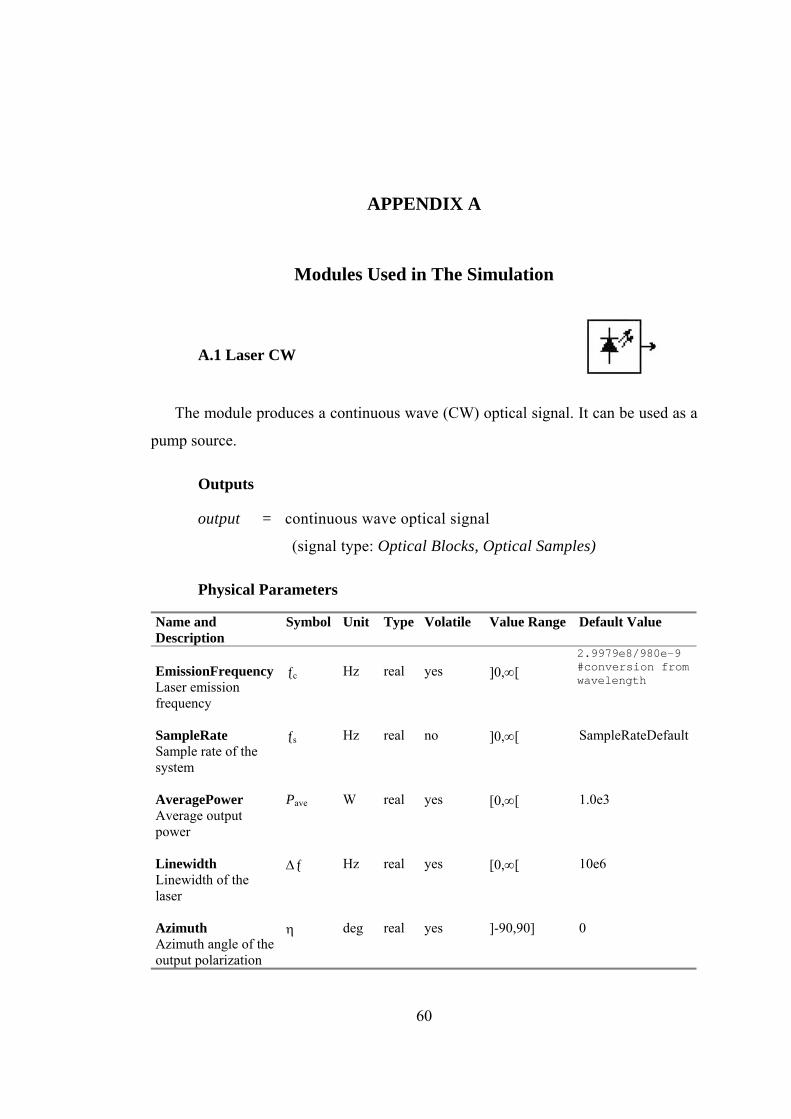
A.1 Laser CW
The module produces a continuous wave (CW) optical signal. It can be used as a
pump source.
Outputs
output = continuous wave optical signal
(signal type: Optical Blocks, Optical Samples)
Physical Parameters
Name and Description
Symbol Unit Type Volatile Value Range Default Value
EmissionFrequency Laser emission frequency
ƒc
Hz
real
yes
]0,∞[
2.9979e8/980e-9 #conversion from wavelength
SampleRate Sample rate of the system
ƒs
Hz
real
no
]0,∞[
SampleRateDefault
AveragePower Average output power
Pave
W
real
yes
[0,∞[
1.0e3
Linewidth Linewidth of the laser
∆ƒ
Hz
real
yes
[0,∞[
10e6
Azimuth Azimuth angle of the output polarization
η
deg
real
yes
]-90,90]
0
60
Ellipticity Ellipticity angle of the output polarization
ε
deg
real
yes
[-45,45]
0
InitialPhase Initial phase
φc
deg
real
no
]-∞,∞[
0
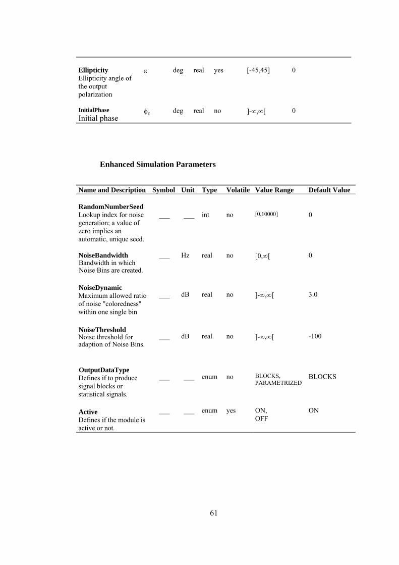
Enhanced Simulation Parameters
Name and Description Symbol Unit Type Volatile Value Range Default Value RandomNumberSeed Lookup index for noise generation; a value of zero implies an automatic, unique seed.
___
___
int
no
[0,10000]
0
NoiseBandwidth Bandwidth in which Noise Bins are created.
___
Hz
real
no
[0,∞[
0
NoiseDynamic Maximum allowed ratio of noise "coloredness" within one single bin
___
dB
real
no
]-∞,∞[
3.0
NoiseThreshold Noise threshold for adaption of Noise Bins.
___
dB
real
no
]-∞,∞[
-100
OutputDataType Defines if to produce signal blocks or statistical signals.
___
___
enum
no
BLOCKS, PARAMETRIZED
BLOCKS
Active Defines if the module is active or not.
___
___
enum
yes
ON, OFF
ON
61
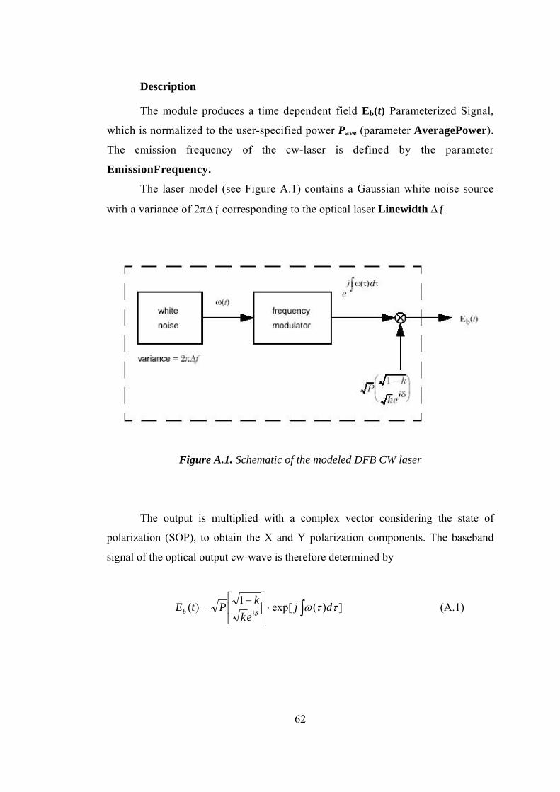
Description
The module produces a time dependent field Eb(t) Parameterized Signal,
which is normalized to the user-specified power Pave (parameter AveragePower).
The emission frequency of the cw-laser is defined by the parameter
EmissionFrequency.
The laser model (see Figure A.1) contains a Gaussian white noise source
with a variance of 2π∆ƒ corresponding to the optical laser Linewidth ∆ƒ.
Figure A.1. Schematic of the modeled DFB CW laser
The output is multiplied with a complex vector considering the state of
polarization (SOP), to obtain the X and Y polarization components. The baseband
signal of the optical output cw-wave is therefore determined by
])(exp[1)( ∫⋅⎥⎦
⎤⎢⎣
⎡ −= ττω
δdj
ekkPtEib (A.1)
62
The SOP is given by the power splitting parameter k (0≤ k ≤ 1) and an
additional phase δ. The relations of k and δ with the Azimuth η and the Ellipticity ε
are given by
( )k
kk21
cos.)1(22tan
−−
=δ
η
δε sin.)1(2)2sin( kk −= (A.2)
With the parameter InitialPhase φc, the user can determine the initial phase of the
optical carrier. The parameter RandomNumberSeed specifies an index of a lookup
table for the generation of the laser phase noise. A value of zero produces a unique
seed to start the noise generator. This assures that each noise field generated in the
simulation is not correlated to all other noise fields, since a unique seed is used for
each noise generation. Note that for user-specified seed values, correlation between
different noise processes can occur.
The parameter OutputDataType defines if the module produces optical BLOCKS,
SAMPLES or PARAMETRIZED signals as output data.
Signal Representation: Individual Samples
Individual Sample Mode is supported by this module.
Boundary Conditions
Both periodic and aperiodic boundary conditions are supported.
Reinitialization Behavior
Multiple Runs:
In the first run, a unique seed is occupied by each module if the start seed value
was chosen to zero. On consecutive runs, the individual random sequence of each
63
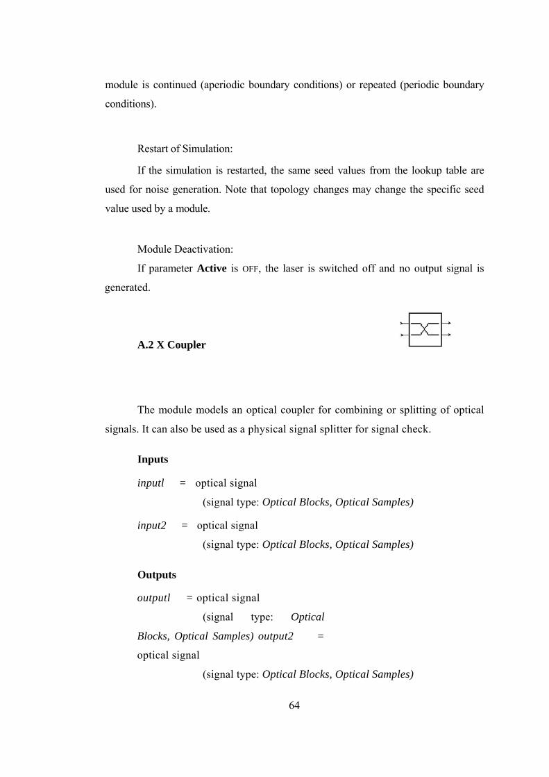
module is continued (aperiodic boundary conditions) or repeated (periodic boundary
conditions).
Restart of Simulation:
If the simulation is restarted, the same seed values from the lookup table are
used for noise generation. Note that topology changes may change the specific seed
value used by a module.
Module Deactivation:
If parameter Active is OFF, the laser is switched off and no output signal is
generated.
A.2 X Coupler
The module models an optical coupler for combining or splitting of optical
signals. It can also be used as a physical signal splitter for signal check.
Inputs
inputl = optical signal
(signal type: Optical Blocks, Optical Samples)
input2 = optical signal
(signal type: Optical Blocks, Optical Samples)
Outputs
outputl = optical signal
(signal type: Optical
Blocks, Optical Samples) output2 =
optical signal
(signal type: Optical Blocks, Optical Samples)
64
Physical Parameters
Name and Description
Symbol Unit Type Volatile Value Range Default Value
ConpleFactor Specifies the cross_couplingcoefficient, from port 1 to port 2.
α
___
real
yes
[0,1]
0.5
In our simulation, same parameter values are used.
Signal Representation: Samples
The cross coupler is defined by its transmission matrix (A.3)
(A.4)
with the CoupleFactor α. E1,in and E2,in are the input electrical fields and E1,out and
E2,out are the output fields at the ports 1 and 2 of the coupler, respectively.
Boundary Conditions
Both, periodic and aperiodic boundary conditions are supported.
65
A.3 X Coupler Bidirectional
The module acts as a bidirectional X Coupler. It is implemented as two
independent X Couplers, one for forward and one for backward direction.
Inputs
inlForward = optical signal
(signal type: Optical Blocks, Optical Samples)
in2Forward = optical signal
(signal type: Optical Blocks, Optical Samples)
inlBackward = optical signal
(signal type: Optical Blocks, Optical Samples)
in2Backward = optical signal
(signal type: Optical Blocks, Optical Samples)
Outputs
outlBackward = optical signal
(signal type: Optical Blocks, Optical Samples)
outlForward = optical signal
(signal type: Optical Blocks, Optical Samples)
out2Backward = optical signal
(signal type: Optical Blocks, Optical Samples)
out2Forward = optical signal
(signal type: Optical Blocks, Optical Samples)
66
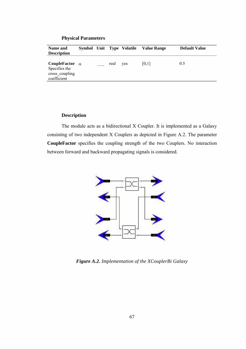
Physical Parameters
Name and Description
Symbol Unit Type Volatile Value Range Default Value
CoupleFactor Specifies the cross_couplingcoefficient
α
___
real
yes
[0,1]
0.5
Description
The module acts as a bidirectional X Coupler. It is implemented as a Galaxy
consisting of two independent X Couplers as depicted in Figure A.2. The parameter
CoupleFactor specifies the coupling strength of the two Couplers. No interaction
between forward and backward propagating signals is considered.
Figure A.2. Implementation of the XCouplerBi Galaxy
67
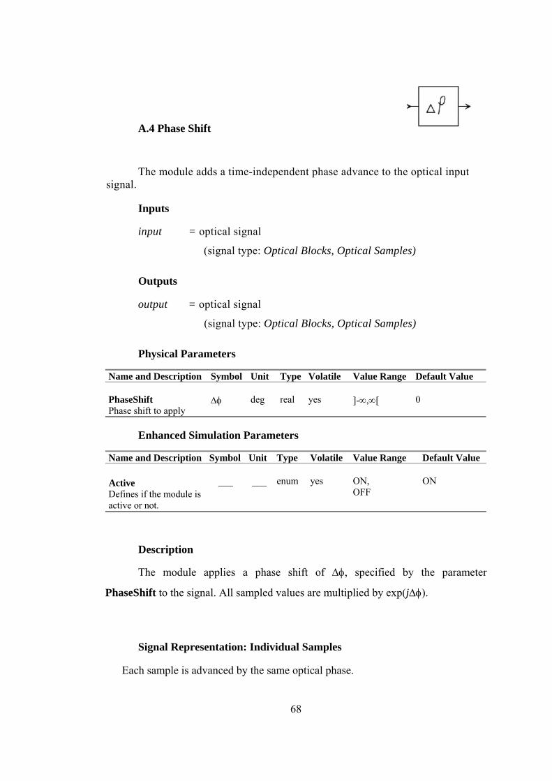
A.4 Phase Shift
The module adds a time-independent phase advance to the optical input signal.
Inputs
input = optical signal
(signal type: Optical Blocks, Optical Samples)
Outputs
output = optical signal
(signal type: Optical Blocks, Optical Samples)
Physical Parameters
Name and Description Symbol Unit Type Volatile Value Range Default Value PhaseShift Phase shift to apply
∆φ
deg
real
yes
]-∞,∞[
0
Enhanced Simulation Parameters
Name and Description Symbol Unit Type Volatile Value Range Default Value Active Defines if the module is active or not.
___
___
enum
yes
ON, OFF
ON
Description
The module applies a phase shift of ∆φ, specified by the parameter
PhaseShift to the signal. All sampled values are multiplied by exp(j∆φ).
Signal Representation: Individual Samples
Each sample is advanced by the same optical phase.
68
A.5 Sine Generator (Electrical)
This module generates an electrical sine waveform superimposed on a
constant bias.
Outputs
output = Output of electrical signal
(signal type: Electrical Blocks, Electrical Samples)
Physical Parameters
Name and Description
Symbol Unit Type Volatile Value Range Default Value
SampleRate Sample rate of the output signal
___
Hz
real
no
]0,∞[a
SampleRateDefault
Amplitude Zero-to-peak amplitude of the output signal.
E0
a.u.
real
yes
[0,∞[a
1.0
Frequency Frequency of output signal.
ƒ
Hz
real
yes
[0, sample rate/2[a
1e8
Phase Initial phase of output signal.
ϕ
deg
real
yes
[0,∞[a
0.0
Bias DC offset of output signal.
Ebias
a.u.
real
yes
]-∞,∞]a
0.0
69
Enhanced Simulation Parameters
Name and Description Symbol Unit Type Volatile Value Range Default Value OutputDataType Defines type of output: Sample Mode or Block Mode..
___
___
enum
no
SAMPLES, BLOCKS
BLOCKS
Active Defines if the module is active or not.
___
___
enum
yes
ON, OFF
ON
Description
This module can be used to generate a sine signal of arbitrary amplitude and
initial phase, as adjusted with Amplitude and Phase, respectively. The frequency
may be chosen from zero Hz (DC) up to a value lower than half the sample rate. A
DC Offset may be applied to the signal using Bias.
The electrical output signal of the module is determined by
)2sin(E 0out ϕπ ++= ftEEbias (A.5)
where Ebias denotes the Bias, ƒ the Frequency and ϕ the initial Phase.
Signal Representation: Individual Samples
If parameter OutputDataType is set to Samples, the module produces an
output signal in Sample Mode, at a sample rate equal to the global variable
SampleModeBandwidth.
70
A.6 Multiple Output Connector (Fork)
Copy input particles to each output.
Inputs
input = Input
(signal type: anytype)
Outputs
output = Output
(signal type: anytype)
Description
This star is generally used to connect a single output port to multiple input
ports. It will be automatically inserted when multiple inputs are connected to the
same output using the graphical interface, or when the "nodeconnect" command is
used in the interpreter. However, there are times when automatically inserted Fork
stars are not desirable. For instance, when there is a delay on one of the arcs, then the
Fork must be inserted by the user explicitly to avoid ambiguity about the location of
the delay. Also, when multi-portholes are used, auto-forking can cause problems. In
this situation, one may get, for example, two outputs and several inputs on the same
net. There is currently no way to automatically decipher what the user intends.
Hence, the Fork star should be inserted explicitly.
71
A.7 Modulator Phase
The module simulates an ideal phase modulator (PM).
Inputs
carrier = optical carrier
(signal type: Optical Blocks, Optical Samples)
data = electrical modulation signal; must be within the range [0,1]
(signal type: Electrical Blocks, Electrical Samples)
Outputs
output = modulated optical signal
(signal type: Optical Blocks, Optical Samples)
Physical Parameters
Name and Description Symbol Unit Type Volatile Value Range Default Value PhaseDeviation Phase difference between marks and spaces
∆φ
deg
real
yes
]-∞,∞[
180
Enhanced Simulation Parameters
Name and Description Symbol Unit Type Volatile Value Range Default Value Active Defines if the module is active or not.
___
___
enum
no
ON, OFF
ON
72
Description
The output signal Eout(t) is given by
Eout(t) = Ein(t) . exp[j∆φ data(t)], (A.6)
where Ein(t) denotes the input optical signal, data(t) represents the electrical
modulation signal, and ∆φ denotes the phase deviation specified by parameter
PhaseDeviation.
The optical power is not affected by the phase modulator.
If the electrical and optical input signals have different sample rates, the
signal that has the lower sample rate is upsampled.
Arbitrary polarization state is allowed for the input optical signal. The output
polarization is the same as the input one.
Signal Representation: Individual Samples
Each sample is processed in the time domain according to (A.6).
Reinitialization Behavior
Module Deactivation:
If parameter Active is OFF, the optical input signals will be passed through
the module without any changes.
73
A.8 Photodiode PIN
The module acts as a PIN photodiode with additive Gaussian white noise sources.
Inputs
input = optical signal
(signal type: Optical Blocks, Optical Samples)
Outputs
output = electrical signal
(signal type: Electrical Blocks, Electrical Samples)
Physical Parameters
Name and Description
Symbol Unit Type Volatile Value Range Default Value
Responsivity Responsivity of the photodiode.
r
A/W
real
yes
[0,2]
1.0
ThermalNoise Thermal noise of additional preamplifier/load resistor.
Nth
HzA
real
yes
[0,100- 10-12 ]
10.0e-12
DarkCurrent Dark current.
id
A
real
yes
[0,10.10-6 ]
0.0
ShotNoise Switch shot noise ON or OFF .
___
___
enum
no
ON, OFF
ON
74
Enhanced Simulation Parameters
Name and Description Symbol Unit Type Volatile Value Range Default Value RandomNumberSeed Lookup index for noise generation; a value of zero implies an automatic, unique seed.
___
___
int
no
[0,10000]
0
Description
The module converts the incident optical field into an electrical signal.
Since at the input, several separated sampled optical bands may be present, all
optical bands are joined to one sampled optical band. Noise Bins falling within
the combined sampled band's bandwidth are added after conversion to random
Gaussian optical fields. The combined optical field E(t) is then converted into an
optical power Ps(t) by taking its modulus squared, and converting to an electrical
signal as described below.
For modeling a PIN photodetector, the process of converting the optical
intensity into an electrical current is described by
i(t) = is(t) + nsh(t) + nth(t) + id. (A.7)
In this equation:
• With the Responsivity r the output signal current is(t) is directly related to
the absorbed optical power Ps(t) by is(t) = r • Ps(t).
nsh denotes the generated ShotNoise current with the one-sided spectral
noise density Nsh in HzA / . The spectral density is determined by
Nsh = 2q.(is+id), (A.8)
if ShotNoise is switched ON.
• nth represents the ThermalNoise caused by the (usually high) photodetector's
internal resistance. The associated one-sided spectral noise density Nth has to be
specified by the user in HzA / .
• id denotes the PIN DarkCurrent.
This is illustrated in Figure A.3.
75
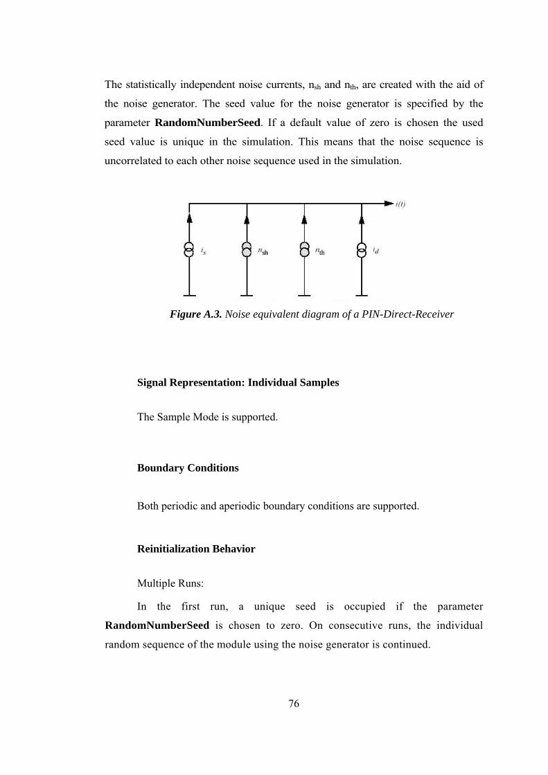
The statistically independent noise currents, nsh and nth, are created with the aid of
the noise generator. The seed value for the noise generator is specified by the
parameter RandomNumberSeed. If a default value of zero is chosen the used
seed value is unique in the simulation. This means that the noise sequence is
uncorrelated to each other noise sequence used in the simulation.
Figure A.3. Noise equivalent diagram of a PIN-Direct-Receiver
Signal Representation: Individual Samples
The Sample Mode is supported.
Boundary Conditions
Both periodic and aperiodic boundary conditions are supported.
Reinitialization Behavior
Multiple Runs:
In the first run, a unique seed is occupied if the parameter
RandomNumberSeed is chosen to zero. On consecutive runs, the individual
random sequence of the module using the noise generator is continued.
76
Restart of Simulation:
If the simulation is restarted, the same seed value from the lookup table is
used for noise generation. Note that topology changes may change the specific seed
value used by a module.
Module Deactivation:
Currently not available.
Error Indications and Warnings
A warning message occurs if only Noise Bins or Parameterized Signals are
available as an input signal.
A.9 Null Source
The module represents a null source for signals of any type. This
module is required to terminate all unused inputs.
Outputs
output = optical or electrical signal
(signal type: Optical Blocks, Optical Samples,
Electrical Blocks, Electrical Samples)
77
Enhanced Simulation Parameters
Name and Description Symbol Unit Type Volatile Value Range
Default Value
OutputSignal Defines if to produce optical or electrical kind of output data.
__
__
enum
no
Electrical, Optical
Optical
OutputDataType Defines whether to generate Block Mode or Sample Mode signal.
__
__
enum
no
Samples, Blocks
Blocks
In our simulation, OutputSignal is ‘Optical’ and OutputDataType is
‘Samples’.
Description
The module is typically used to provide subsequent modules with a null
input. The parameter OutputSignal chooses the output data type. Depending on
the input type of the connected module, the type has to be chosen properly to
prevent data type mismatching to the input of the following module. The
parameter OutputDataType chooses the data type of the signal. It can be block
mode or sample mode.
A.10 Ground
The Ground module discards input signals. This module is required to
terminate unused output ports of all modules. The Design Assistant AutoGrounds
will do this automatically.
Inputs
input (multiple) = optical or electrical signal
(signal type: anytype)
78
Description
To discard signals of any type which are of no further interest, this module
can be applied as the termination (data sink).
Signal Representation: Individual Samples
The sample mode is supported by this module.
Boundary Conditions
Both periodic and aperiodic boundary conditions are supported.
A.11 Time Domain Fiber
The TimeDomainFiber is designed to be used with Sample Mode or
Aperiodic Block Mode components as it runs with Aperiodic Boundary
Conditions. It can be used to model self- and cross- phase modulation, four-
wave mixing, stimulated Raman scattering, second- and third-order group
velocity dispersion, and frequency-dependent attenuation. A constant state of
linear polarization is assumed, as with most components in this tool.
Inputs
leftlnput = optical signal input
(signal type: Optical Samples, Optical Blocks)
Outputs
rightOutput = optical signal output
(signal type: Optical Samples, Optical Blocks)
79
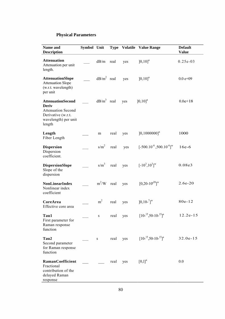
Physical Parameters
Name and Description
Symbol Unit Type Volatile Value Range Default Value
Attenuation Attenuation per unit length.
___
dB/m
real
yes
]0,10]a
0.25e-03
AttenuationSlope Attenuation Slope (w.r.t. wavelength) per unit
___
dB/m2
real
yes
]0,10]a
0.0 e+09
AttenuationSecondDeriv Attenuation Second Derivative (w.r.t. wavelength) per unit length
___
dB/m3
real
yes
]0,10]a
0.0e+18
Length Fiber Length
___
m
real
yes
]0,1000000]a
1000
Dispersion Dispersion coefficient.
___
s/m2
real
yes
[-500.10-6 ,500.10-6]w
16e-6
DispersionSlope Slope of the dispersion
___
s/m3
real
yes
[-103,103]w
0.08e3
NonLinearIndex Nonlinear index coefficient
___
m2/W
real
yes
[0,20-10'20]w
2.6e-20
CoreArea Effective core area
___
m2
real
yes
]0,10-7]w
80e-12
Tau1 First parameter for Raman response function
___
s
real
yes
[10-15,50-10-15]a
12.2e-15
Tau2 Second parameter for Raman response function
___
s
real
yes
[10-15,50-10-15]a
32.0e-15
RamanCoefficient Fractional contribution of the delayed Raman response
___
___
real
yes
[0,l]a
0.0
80
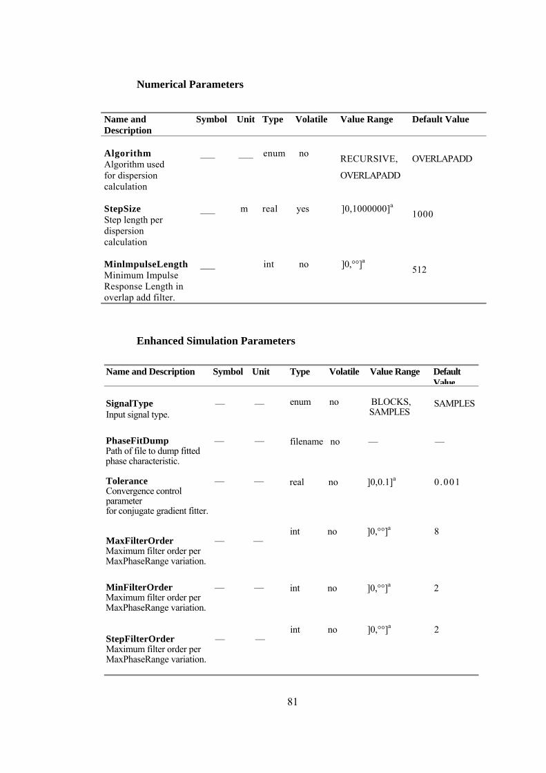
Numerical Parameters
Name and Description
Symbol Unit Type Volatile Value Range Default Value
Algorithm Algorithm used for dispersion calculation
___
___
enum
no
RECURSIVE,
OVERLAPADD
OVERLAPADD
StepSize Step length per dispersion calculation
___
m
real
yes
]0,1000000]a
1000
MinlmpulseLength Minimum Impulse Response Length in overlap add filter.
___
int
no
]0,°°]a
512
Enhanced Simulation Parameters
Name and Description Symbol Unit Type Volatile Value Range Default Value
SignalType — — Input signal type.
enum no BLOCKS, SAMPLES
SAMPLES
PhaseFitDump — — Path of file to dump fitted phase characteristic.
filename no — —
Tolerance — — Convergence control parameter for conjugate gradient fitter.
real no ]0,0.1]a 0 .001
MaxFilterOrder — — Maximum filter order per MaxPhaseRange variation.
int no ]0,°°]a 8
MinFilterOrder — — Maximum filter order per MaxPhaseRange variation.
int no ]0,°°]a 2
StepFilterOrder — — Maximum filter order per MaxPhaseRange variation.
int no ]0,°°]a 2
81
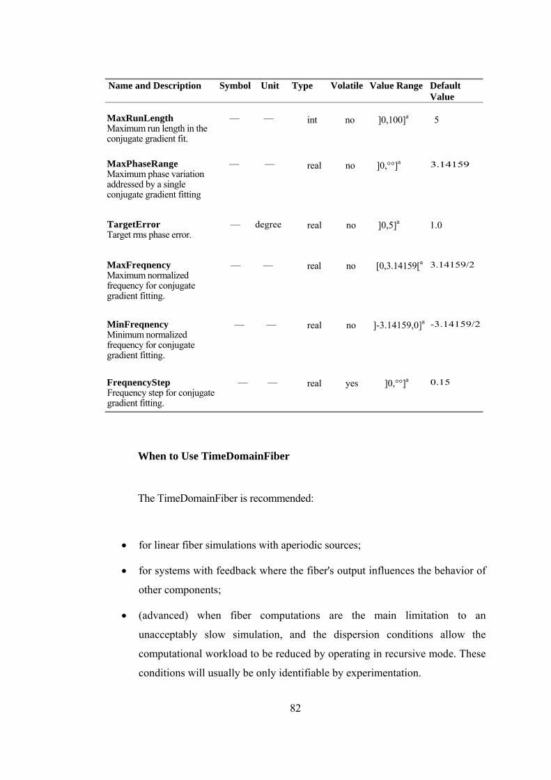
Name and Description Symbol Unit Type Volatile Value Range Default Value
MaxRunLength — — Maximum run length in the conjugate gradient fit.
int no ]0,100]a
5
MaxPhaseRange — — Maximum phase variation addressed by a single conjugate gradient fitting
real no ]0,°°]a
3.14159
TargetError — degree Target rms phase error.
real no ]0,5]a 1.0
MaxFreqnency — — Maximum normalized frequency for conjugate gradient fitting.
real no [0,3.14159[a 3.14159/2
MinFreqnency — — Minimum normalized frequency for conjugate gradient fitting.
real no ]-3.14159,0]a -3.14159/2
FreqnencyStep — — Frequency step for conjugate gradient fitting.
real yes ]0,°°]a 0.15
When to Use TimeDomainFiber
The TimeDomainFiber is recommended:
• for linear fiber simulations with aperiodic sources;
• for systems with feedback where the fiber's output influences the behavior of
other components;
• (advanced) when fiber computations are the main limitation to an
unacceptably slow simulation, and the dispersion conditions allow the
computational workload to be reduced by operating in recursive mode. These
conditions will usually be only identifiable by experimentation.
82
The TimeDomainFiber is not recommended for quick and dirty simulations unless
you have considerable experience with the TimeDomainFiber model. Generally,
finding a sensible choice of internal parameters means that simulations involving
TimeDomainFiber require more patience and work to give sound results than do
simulations where another fiber model is applicable.
Do not use TimeDomainFiber in recirculating-loops. The TimeDomainFiber
model maintains its own internal state and thus assumes its input is from a particular
physical point in the network. The output is dependent on the input history, which
will be distorted and unphysical if it is taken from several different physical network
points, as will occur within loops. The same restriction applies to many sample-mode
models which have their own internal memories, such as the LaserTLM family.
Module Delay
A feature of TimeDomainFiber to note is its delay of signals. This is in
contrast to the behavior of the module FiberNLS, because FiberNLS calculates
dispersive effects based on a Fourier transform of the entire time window and can
thus strip away common-mode delays through the system. Therefore dispersion with
zero slope will be calculated by FiberNLS to have a zero delay (input and output
pulses thus centered at the same position). Because FiberNLS addresses the whole
time window in one step, it can implement this non-causal behavior to keep all the
pulses centered at the same place. In contrast, TimeDomainFiber uses time domain
filters, which are necessarily causal and hence it can never completely strip away the
common-mode pulse delay as FiberNLS can [20].
83
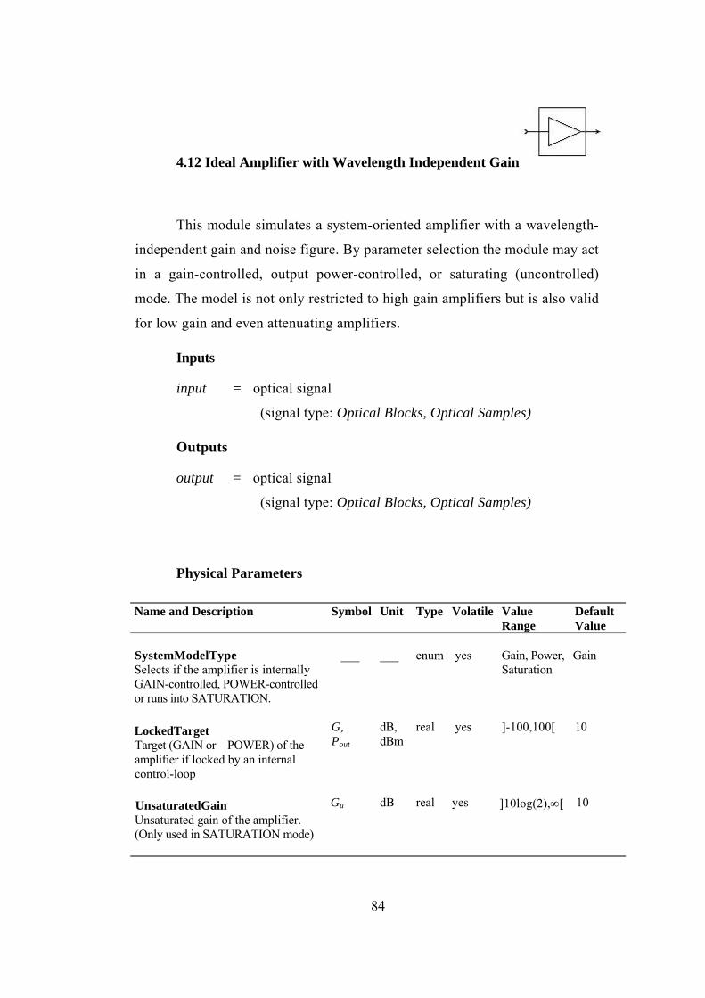
4.12 Ideal Amplifier with Wavelength Independent Gain
This module simulates a system-oriented amplifier with a wavelength-
independent gain and noise figure. By parameter selection the module may act
in a gain-controlled, output power-controlled, or saturating (uncontrolled)
mode. The model is not only restricted to high gain amplifiers but is also valid
for low gain and even attenuating amplifiers.
Inputs
input = optical signal
(signal type: Optical Blocks, Optical Samples)
Outputs
output = optical signal
(signal type: Optical Blocks, Optical Samples)
Physical Parameters
Name and Description Symbol Unit Type Volatile Value Range
Default Value
SystemModelType Selects if the amplifier is internally GAIN-controlled, POWER-controlled or runs into SATURATION.
___
___
enum
yes
Gain, Power, Saturation
Gain
LockedTarget Target (GAIN or POWER) of the amplifier if locked by an internal control-loop
G, Pout
dB, dBm
real
yes
]-100,100[
10
UnsaturatedGain Unsaturated gain of the amplifier. (Only used in SATURATION mode)
Gu dB real yes ]10log(2),∞[ 10
84
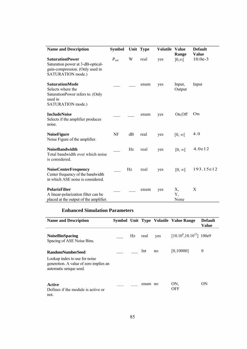
Name and Description Symbol Unit Type Volatile Value Range
Default Value
SaturationPower Saturation power at 3-dB-optical-gain-compression. (Only used in SATURATION mode.)
Psat W real yes ]0,∞[ 10.0e-3
SaturationMode Selects where the SaturationPower refers to. (Only used in SATURATION mode.)
___
___
enum
yes
Input, Output
Input
IncludeNoise Selects if the amplifier produces noise.
___
___
enum
yes
On,Off
On
NoiseFigure Noise Figure of the amplifier.
NF
dB
real
yes
[0, ∞[
4.0
NoiseBandwidth Total bandwidth over which noise is considered.
___
Hz
real
yes
[0, ∞[
4.0e12
NoiseCenterFreqnency Center frequency of the bandwidth in which ASE noise is considered.
___
Hz
real
yes
[0, ∞[
193.15e12
PolarizFilter A linear-polarization filter can be placed at the output of the amplifier.
___
___
enum
X, Y, None
X yes
Enhanced Simulation Parameters
Name and Description Symbol Unit Type Volatile Value Range Default Value
NoiseBinSpacing Spacing of ASE Noise Bins.
___
Hz
real
yes
[10.106,10.1012]
100e9
RandomNumberSeed Lookup index to use for noise generetion. A value of zero implies an automatic unique seed.
___
___
Int
no
[0,10000]
0
Active Defines if the module is active or not.
___
___
enum
no
ON, OFF
ON
85
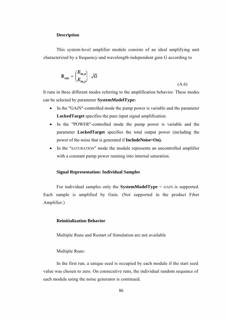
Description
This system-level amplifier module consists of an ideal amplifying unit
characterized by a frequency-and wavelength-independent gain G according to
(A.6)
It runs in three different modes referring to the amplification behavior. These modes
can be selected by parameter SystemModelType:
• In the "GAiN"-controlled mode the pump power is variable and the parameter
LockedTarget specifies the pure input signal amplification.
• In the "POWER"-controlled mode the pump power is variable and the
parameter LockedTarget specifies the total output power (including the
power of the noise that is generated if IncludeNoise=On).
• In the "SATURATION" mode the module represents an uncontrolled amplifier
with a constant pump power running into internal saturation.
Signal Representation: Individual Samples
For individual samples only the SystemModelType = GAIN is supported.
Each sample is amplified by Gain. (Not supported in the product Fiber
Amplifier.)
Reinitialization Behavior
Multiple Runs and Restart of Simulation are not available
Multiple Runs:
In the first run, a unique seed is occupied by each module if the start seed
value was chosen to zero. On consecutive runs, the individual random sequence of
each module using the noise generator is continued.
86
Restart of Simulation:
If the simulation is restarted again, the same seed values from the lookup
table are used for noise generation. Note that topology changes may change the
specific seed value used by a module.
Module Deactivation:
If Active is OFF, the input signal is passed through to the output without
any changes.
Comments
The Noise Figure is allowed to fall below NFmin, but an instructive warning
is thrown.
87