SIMULATION OF WINDBORNE DEBRIS TRAJECTORIES by NING

SIMULATION OF WINDBORNE DEBRIS TRAJECTORIES

by

NING LIN, B.S.

A THESIS

IN

CIVIL ENGINEERING

Submitted to the Graduate Faculty of Texas Tech University in

Partial Fulfillment of the Requirements for

the Degree of

MASTER OF SCIENCE

IN

CIVIL ENGINEERING

Approved

Chris W. Letchford Chairperson of the Committee

Xinzhong Chen

Accepted

John Borrelli Dean of the Graduate School

August, 2005

ii

ACKNOWLEDGEMENTS

I would like to express my most sincere gratitude to my mentor, Dr. Chris W.

Letchford, for his constant guidance, encouragement, and support throughout my

graduate study. His interactive teaching, openmindedness, and kindness have been

inspiring to me.

I am grateful to Dr. John D. Holmes for his instruction, particularly for his advice

concerning the development of experimental models based on theoretical equations, and

the numerical solutions he provided to use for comparisons in this research.

My thanks also go to Dr. Xinzhong Chen for his insightful comments, and to Drs.

Douglas A. Smith and Kishor C. Mehta for their support throughout my graduate study at

Texas Tech. I am indebted as well to Dr. Ahsan Kareem of the University of Notre Dame

and Dr. Yukio Tamura at Tokyo Polytechnic University for their valuable advice.

This study was conducted under the auspices of the NIST/TTU Wind Storm

Mitigation Initiative. I am very grateful to Mr. Taylor Gunn, Mr. Dejiang Chen, and Ms.

Shannon Smith, for their assistance in carrying out these extensive experiments.

I would also like to thank Dr. Sharon Myers of the Department of Classical and

Modern Languages for her great guidance in my English learning and her cheerful

encouragement of my pursuit of excellence.

My deepest appreciation is reserved for my family. I want to thank my fiance, Lei

Yang, for his love and moral support from my home country of China. I am extremely

grateful to my parents, Baoshuo Lin and Anning Luo. Their enduring love and trust are

the foundations of my every achievement. I dedicate this thesis to them.

iii

TABLE OF CONTENTS

ACKNOWLEDGEMENTS ............................................................................................... ii

ABSTRACT ........................................................................................................................v

LIST OF TABLES ............................................................................................................ vi

LIST OF FIGURES ......................................................................................................... vii

LIST OF PUBLICATIONS ................................................................................................x

CHAPTER

I. INTRODUCTION ........................................................................................................1

1.1 Debris Identification .........................................................................................3

1.2 Debris Flight Initiation ......................................................................................4

1.3 Debris Flight Trajectory ....................................................................................6

1.4 Risk Analysis of Windborne Debris ...............................................................10

1.5 Statement of the Problem ................................................................................15

1.6 Research Objectives ........................................................................................15

1.7 Organization of the Thesis ..............................................................................16

II. SIMULATION OF WINDBORNE DEBRIS TRAJECTORY...................................18

2.1 Introduction .....................................................................................................18

2.2 Wind-tunnel Test ............................................................................................19

2.3 Full-scale Experiment .....................................................................................24

2.4 Data Analysis and Interpretation ....................................................................26

III. SIMULATION RESULTS AND DISCUSSION .....................................................38

3.1 Introduction .....................................................................................................38

3.2 Characteristics of Debris Trajectory ...............................................................39

3.3 Non-dimensional Horizontal Debris Trajectory .............................................60

3.4 Comparison of Full-scale and Model-scale Simulations ................................70

3.5 Application to Debris Impact Criteria .............................................................75

iv

IV. SUMMARY AND RECOMMENDATIONS ..........................................................80

4.1 Summary .........................................................................................................80

4.2 Recommendations for Further Research .........................................................81

BIBLIOGRAPHY .............................................................................................................82

v

ABSTRACT

Windborne debris is possibly the major cause of building damage and destruction

in strong wind events such as hurricanes and tornadoes. It has been long recognized that

fast-flying debris can penetrate building envelopes, inducing internal pressurization and

doubling the net loading on roofs, side walls, and leeward walls. Consequently, failed

roofing structures, damaged wall cladding panels, and broken glass become debris

sources, threatening downwind areas. Knowledge of debris aerodynamics is necessary for

proper estimation of debris trajectory and for establishment of rational debris impact

criteria.

This research aims to investigate the aerodynamics of flying debris through

simulating debris trajectories. Extensive wind-tunnel tests on 3D (compact-like), 2D

(plate-like), and 1D (rod-like) debris are carried out in the Texas Tech University wind

tunnel. The simulation procedure is introduced. Full-scale simulation is explored,

employing a C-130 Hercules aircraft to generate strong winds.

Three categories of parameters affecting debris trajectories are investigated: wind

field, debris properties, and debris initial support. It is determined that although many

parameters influence debris trajectory in the vertical direction, the Tachikawa parameter

K (1983) governs the horizontal trajectory of debris. Aerodynamic functions for debris

horizontal trajectory are established based on both experimental data and theoretical

equations of debris motion. These functions can be used to predict debris horizontal

speed (at a given flight distance) and flight distance (for a given flight time).

The application of these functions in debris impact criteria is discussed. The

incorporation of these functions into debris risk analysis is recommended for the further

research.

vi

LIST OF TABLES

2.1 2D-plate models used in free flight tests in wind tunnel ............................................22

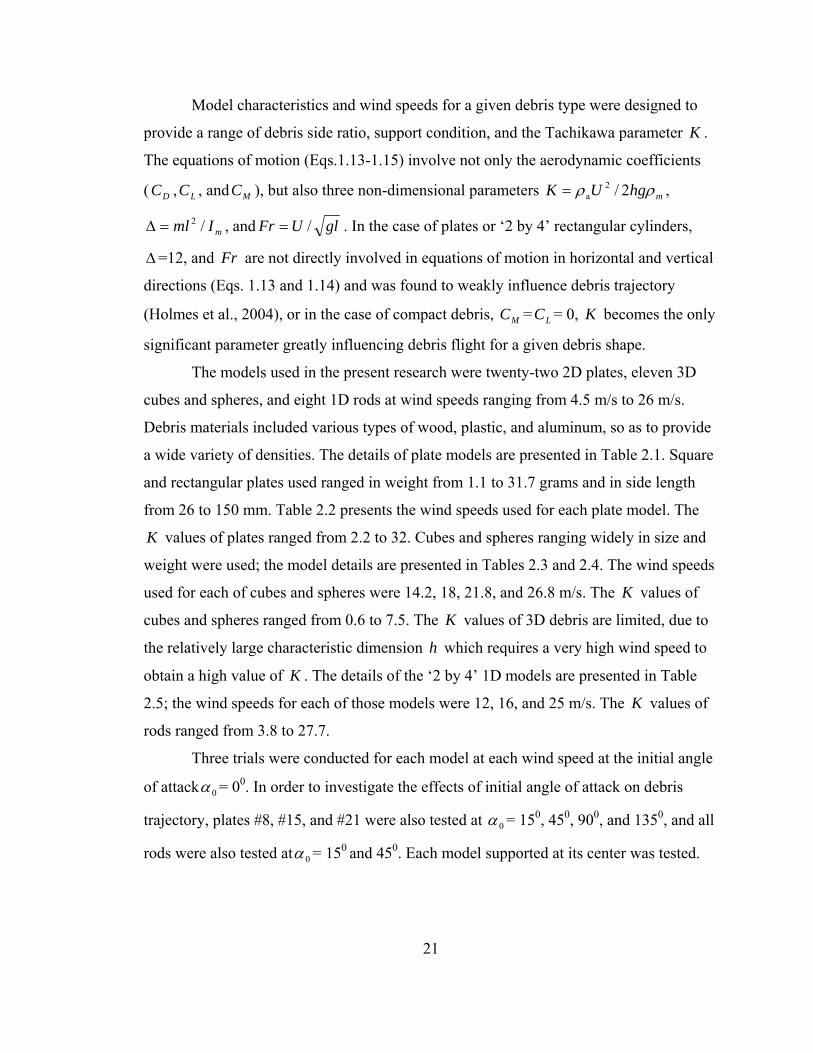
2.2 Wind speeds in free flight tests of plate models in wind tunnel .................................23

2.3 3D-cube models used in free flight tests in wind tunnel .............................................23

2.4 3D-sphere models used in free flight tests in wind tunnel ..........................................24

2.5 1D-rod models used in free flight tests in wind tunnel ...............................................24

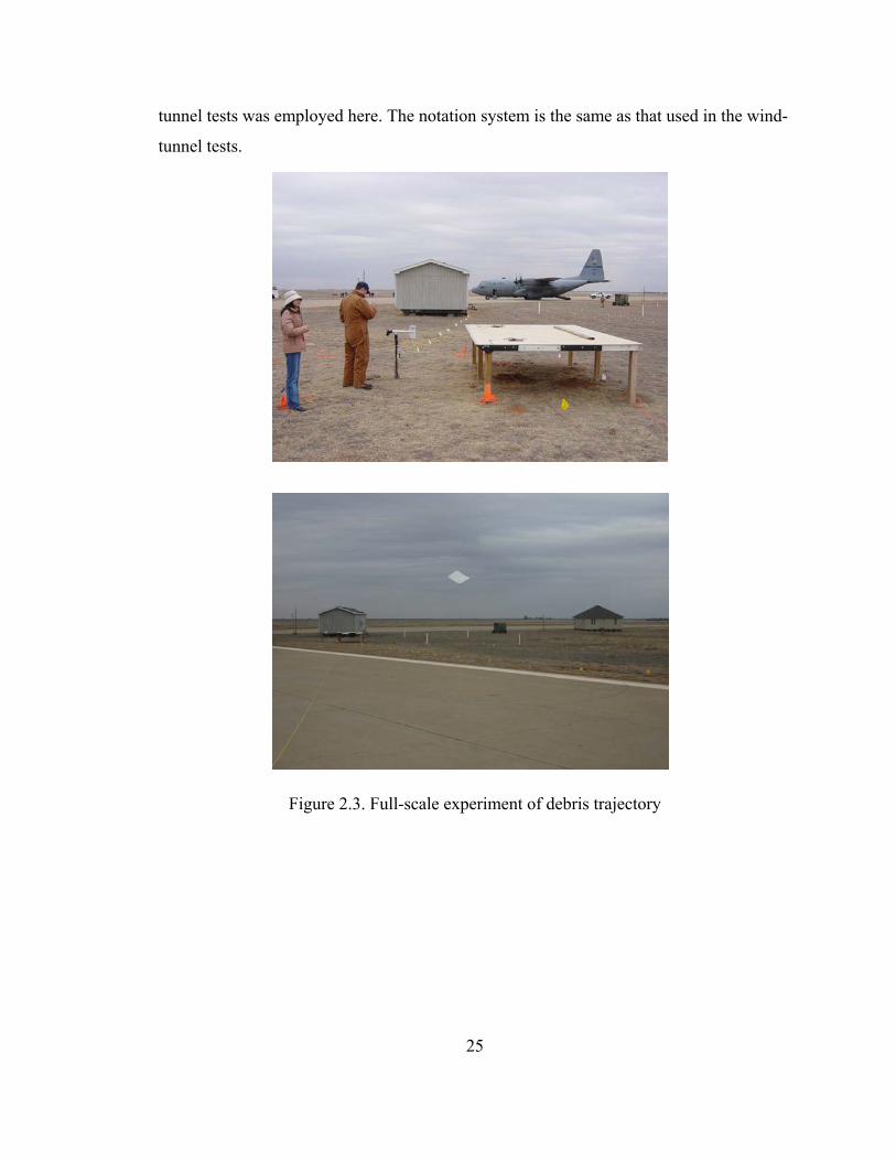
2.6 Details of full-scale debris ..........................................................................................26

vii

LIST OF FIGURES

2.1 Test setup in wind tunnel ............................................................................................19

2.2 Debris launch support in wind tunnel .........................................................................20

2.3 Full-scale experiment of debris trajectory ..................................................................25

2.4 Analysis of debris trajectories (Plate #8, U=9.1 m/s, α0 = 00) ....................................28

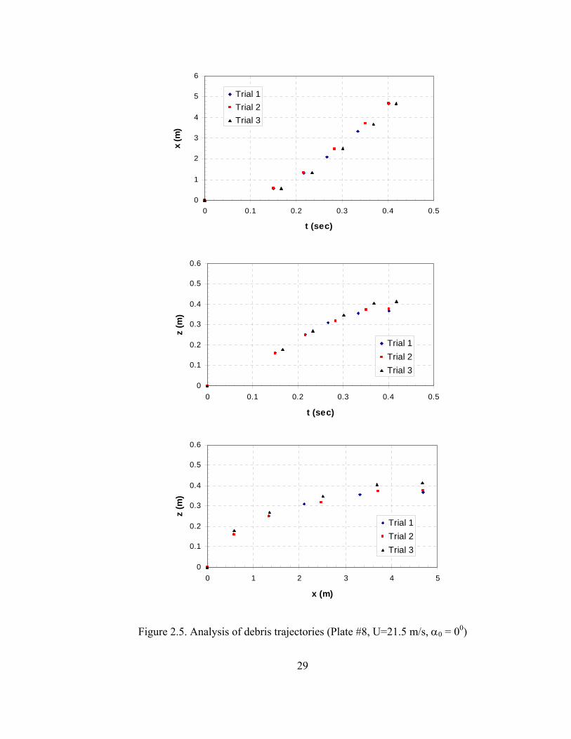
2.5 Analysis of debris trajectories (Plate #8, U=21.5 m/s, α0 = 00) ..................................29

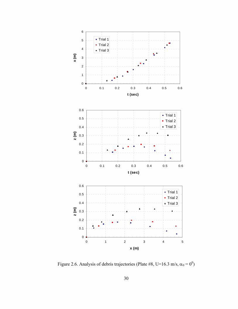
2.6 Analysis of debris trajectories (Plate #8, U=16.3 m/s, α0 = 00) ..................................30

2.7 Calculation of debris horizontal and resultant velocities ............................................31

2.8 Analysis of debris horizontal velocity (Plate #8, U=9.1 m/s, α0 = 00) .......................32

2.9 Analysis of debris vertical velocity (Plate #8, U=9.1 m/s, α0 = 00) ............................33

2.10 Non-dimensional analysis of debris displacements (Plate #8, K =2.1, Fr =8.9 x 10-3, α0 = 00) ...............................................................35

2.11 Non-dimensional analysis of debris horizontal velocity (Plate #8, K =2.1, Fr =8.9 x 10-3, α0 = 00) ...............................................................36

2.12 Non-dimensional analysis of debris vertical velocity (Plate #8, K =2.1, Fr =8.9 x 10-3, α0 = 00) ...............................................................37

3.1 Plate trajectories at different wind speeds (Plate #8, ma ρρ / =0.0015, BD / =1, BDh / =4%, Bb / =24%, 0α =00, s -center) ...40

3.2 Plate trajectories affected by debris density (U = 12.5m/s, BD / =1, BDh / =4%, Bb / =24%, 0α =00, s -center) ........................40

3.3 Plate trajectories affected by geometrical feature BDh / (U = 18.1m/s, ma ρρ / =0.0015, BD / =1, Bb / =24%, 0α =00, s -center) ....................41

3.4 Plate trajectories affected by mhgUK ρρ 2/2a=

( BD / =1, Bb / =24%, 0α =00, s -center) ......................................................................41

3.5 Plate trajectories affected by geometrical feature BD / ..............................................42

3.6 Plate trajectories affected by relative support dimension Bb /

( K =7.6, BD / =1, 0α =00, s -center) ...........................................................................43

3.7 Plate trajectories affected by support place s ( K =3.37, BD / =1, Bb / =43%, 0α =00) ......................................................................44

viii

3.8 Variations in mode of motion and trajectory with initial angle of attack 0α (Plate #8, BD / =1, Bb / =24%, s -center) ...................................................................45

3.9 Variations in mode of motion and trajectory with initial angle of attack 0α (Plate #15, BD / =0.42, Bb / =15%, s -center) ............................................................46

3.10 Variations in mode of motion and trajectory with initial angle of attack 0α (Plate #21, BD / =2.4, Bb / =36%, s -center) ............................................................47

3.11 Horizontal plate trajectories affected by mhgUK ρρ 2/2a=

( BD / =1, Bb / =24%, 0α =00, s -center) ....................................................................49

3.12 Horizontal plate trajectories affected by side ratio ( ≥BD / 1) ( K =6.7, Bb / =33%, 0α =00, s -center) .....................................................................50

3.13 Horizontal plate trajectories affected by side ratio ( ≤BD / 1) ( K =6.7, Bb / =15-20%, 0α =00, s -center) ..............................................................51

3.14 Horizontal plate trajectories affected by Bb / ( K =7.6, BD / =1, 0α =00, s -center) .........................................................................52

3.15 Horizontal plate trajectories affected by s ( K =3.37, BD / =1, Bb / =43%, 0α =00) ....................................................................53

3.16 Horizontal trajectories affected by initial angle of attack 0α (Plate #8, BD / =1, K =5.9, Bb / =24%, s -center) ....................................................54

3.17 Horizontal trajectories affected by initial angle of attack 0α (Plate #8, BD / =1, K =11, Bb / =24%, s -center) .....................................................55

3.18 Horizontal trajectories affected by initial angle of attack 0α (Plate #15, BD / =0.42, K =4.5, Bb / =15%, s -center) .............................................56

3.19 Horizontal trajectories affected by initial angle of attack 0α (Plate #15, BD / =0.42, K =12.5, Bb / =15%, s -center) ...........................................57

3.20 Horizontal trajectories affected by initial angle of attack 0α (Plate #21, BD / =2.4, K =4.5, Bb / =36%, s -center) ...............................................58

3.21 Horizontal trajectories affected by initial angle of attack 0α (Plate #21, BD / =2.4, K =11.2, Bb / =36%, s -center) .............................................59

3.22 Non-dimensional plate trajectories in the horizontal direction ( K =2) ....................61


ix



3.26 Horizontal trajectory of 2D (plate) debris ( pC = 0.911) ............................................67

3.27 Horizontal trajectory of 3D (compact) debris ( cC = 0.809, sC =0.496) ......................68

3.28 Horizontal trajectory of 1D (rod) debris ( rC =0.801) ................................................69

3.29 u versus xK of plates with ≤BD / 1 (above) and BD / >1 (below) .........................71

3.30 xK versus tK of plates with ≤BD / 1 (above) and BD / >1 (below) .......................72

3.31 Comparison of debris trajectories from wind-tunnel (above) and full-scale (below) tests .......................................................................................73

3.32 Comparison of debris velocities from wind-tunnel (above) and full-scale (below) tests ........................................................................................74

3.33 Comparison of debris horizontal trajectories from wind-tunnel and full-scale tests ........................................................................75

3.34 Trajectory of a concrete tile (300 x 300 x 15mm, 3.1kg, 0α =00) .............................77

3.35 Trajectory of a steel ball (8mm, 2g) ..........................................................................77

3.36 Trajectory of a ‘2 by 4’ missile (2.4 x 0.1x 0.05m, 4.1kg, 0α =00) ..........................78

3.37 Trajectory of a ‘2 by 4’ missile (4.0 x 0.1 x 0.05m, 6.8kg, 0α =00) .........................78

3.38 Comparison of horizontal speed and resultant speed of plates ( pC = 0.911) .............79

3.39 Comparison of horizontal speed and resultant speed of rods ( rC = 0.801) ................79

x

LIST OF PUBLICATIONS

Journal Papers under Review

1. Ning Lin, John D. Holmes, and Chris W. Letchford (2005). Trajectories of windborne debris and applications to impact testing. Journal of Structural Engineering (ASCE).

2. Ning Lin, Chris W. Letchford, and John D. Holmes (2005). Investigations of plate-

type windborne debris, I. Experiments in wind tunnel and full-scale. Journal of Wind Engineering and Industrial Aerodynamics.

3. John D. Holmes, Chris W. Letchford and Ning Lin (2005). Investigations of plate-

type windborne debris, II. Computed trajectories. Journal of Wind Engineering and Industrial Aerodynamics.

Journal Papers Published

4. Ning Lin, Chris W. Letchford, Yukio Tamura, Bo Liang, and Osamu Nakamura (2005). Characteristics of wind forces on tall buildings. Journal of Wind Engineering and Industrial Aerodynamics, 93, 217-242.

5. Lin Ning, Liang Bo, Yukio Tamura (2003), “Experimental investigation on local

wind force coefficients and power spectra of high-rise buildings.” Chinese Journal of Vibration Engineering, Vol.16, No.4.

6. Huang Hengwei, Zhang Yaoting, Qiu Jisheng, Lin Ning (2002), “The application of

neural network to forecast the concrete strength”, Journal of Huazhong University of Science and Technology, March, 2002.

7. Zhang Yaoting, Lei Pingan, Liu Zaihua, Lin Ning (2001), “Research on practicability

and feasibility for a new-type of tuned mass damper system”, Journal of China University of Geosciences, December, 2001.

Conference Proceedings

8. Ning Lin, Chris W. Letchford, and Taylor Gunn (2005). Investigation of the flight mechanics of 1D (rod-like) debris. Fourth European & African Conference on Wind Engineering (EACWE2005), Prague, Czech Republic, July 11 – 15, 2005.

9. Ning Lin, Chris W. Letchford, and John D. Holmes (2005). Experimental investigation of trajectory of windborne debris with applications to debris impact criteria. Tenth Americas Conference on Wind Engineering (10ACWE), Baton Rouge, Louisiana, USA, June 1-4, 2005.

xi

10. John D. Holmes, Chris W. Letchford, and Ning Lin (2005). Trajectories of windborne debris of the plate-type. Tenth Americas Conference on Wind Engineering (10ACWE), Baton Rouge, Louisiana, USA, June 1-4, 2005.

11. Ning Lin, Chris W. Letchford, and John D. Holmes (2004). Aerodynamics of 2D wind-borne debris in wind-tunnel and full-scale tests. 6th UK Conference on Wind Engineering, Cranfield University, United Kingdom, September 15-17, 2004.

12. Ning Lin, Chris W. Letchford, and John D. Holmes (2004). Wind tunnel and full-scale tests of 2D windborne debris. The International Conference on Storms and the Annual National Conferences of the Australian Meteorological and Oceanographic Society (AMOS) and the Meteorological Society of New Zealand (MSNZ), Brisbane, Australia, July 5-9, 2004.

13. Ning Lin, Chris W. Letchford, and John D. Holmes (2004). Investigation of 2D wind-borne debris in wind-tunnel and full-scale tests. 11th Australian Wind Engineering Society Workshop, Darwin, Australia, June 28-30, 2004.

14. Ning Lin, Osamu Nakamura, Bo Liang, and Yukio Tamura (2003). Local wind forces

acting on tall buildings. Eleventh International Conference on Wind Engineering (11ICWE), Lubbock, Texas, June 2-5, 2003.

1

CHAPTER I

INTRODUCTION

Windborne debris is possibly the major cause of building damage and destruction

in strong wind events such as hurricanes and tornadoes. Various debris sources have been

observed in the environment: tree branches, signboards, communication antennas, fence

posts, utility poles, storage tanks, and cars. Other prevalent debris are less well fixed

building components or damaged structural members, which can be picked up by strong

winds. These debris include roof gravel, roof sheathing, roof tiles, and timber roof beams.

A worst case is that of strong winds passing by structures under construction, where large

amounts of structural materials, framing members, and scaffold poles become airborne.

As a result, fast-flying debris penetrate building envelopes, inducing internal

pressurization and doubling the net loading on roofs, side walls, and leeward walls.

Consequently, failed roofing structures, damaged wall cladding panels, and broken glass

become debris sources, threatening downwind areas.

In the 1970’s, when the safety of nuclear power plants was of great concern,

McDonald (1976) claimed that the biggest problem in tornado-resistant design of nuclear

power plants and structures is protection from missiles. Missile penetration of those

structures housing radioactive materials poses considerable danger to the environment.

Windborne debris was also considered a critical design factor for other structures: above-

ground shelters, schools, and hospitals, where the protection of people is the primary

concern (McDonald, 1976). In modern urban areas, windows and architectural glazing

systems of tall buildings are among the structures which are most vulnerable to

windborne debris. Minor (1994) illustrated the serious window damage caused by

windborne debris in severe windstorms over a twenty year period, including Hurricane

Alicia, in Houston, Texas in August, 1983, and Hurricane Andrew in Florida, in August,

1992. Recently, Lee and Wills (2002) reported on the significant glazing damage to one

of Asia’s tallest buildings, Central Plaza, Hong Kong, during Typhoon York, in

September 1999.

2

Direct and indirect damage and losses caused by windborne debris have long been

recognized. Building envelopes are required to be designed against windborne debris in

hurricane and tornado zones. However, how strong the building envelopes should be built

to resist debris impact has been an issue. Although a large number of impact tests have

been conducted to decide the required strength of various materials to resist certain debris

impacts (e.g., McDonald, 1990; Minor, 1994; McDonald, 1999), in practice, the

properties and velocities of debris impacting structures are uncertain. In order to address

this problem, the following questions need to be answered: what speed does debris

become airborne? Does airborne debris impact the building of interest, and if so, what is

the impact velocity?

Although research on these questions has been ongoing since the early 1970’s,

there have been few articles on this topic compared with those on wind loading. Holmes

(2003) compared windborne debris to ‘the forgotten land’ in his keynote address to the

Eleventh International Conference on Wind Engineering (Lubbock, Texas, 2003). More

research on this topic is necessary.

Most of the studies fall into two categories: flight initiation and flight trajectory,

both of which involve debris aerodynamics. Investigation of debris flight initiation or

generation includes surveying debris sources and their restraining conditions. The

aerodynamics coefficients of static debris, which greatly affect the flight initiation, can be

determined through general wind-tunnel tests. Following release, the aerodynamic

characteristics of flying debris, however, are much more complex. The present study

applies controlled wind-tunnel simulation to investigate the aerodynamic characteristics

of flying debris so as to predict debris trajectory. The experimental data produced here

can be used to establish rational debris impact criteria.

Studies of debris classification and flight initiation are reviewed in Sections 1.1

and 1.2, respectively. Previous studies of debris trajectory are reviewed in Section 1.3.

Established frameworks of debris risk analysis and risk-based design are reviewed in

Section 1.4. The limited work that has been published, however, provides significant

information and guides the present research. Section 1.5 states the problems the present

3

study aims to address. Section 1.6 specifies the objectives and scope of this research.

Section 1.7 presents the organization of this thesis.

1.1 Debris Identification

Identifying debris is the first step in solving the debris damage problem. Over

thirty years of documented windstorm damage experiences found in the files of the

Institute for Disaster Research at Texas Tech University reveal the major types and

characteristics of actual debris. For research and design purposes, however, debris have

to be identified by their physical properties.

McDonald and Kiesling (1988) categorized windborne debris as light-, medium-,

and heavy-weight, according to their observed damage performance. Light-weight

missiles, which primarily break glass or damage building finishes, include roof gravel,

sheet metal panels, and small tree branches. Medium-weight missiles, which can

perforate ordinary wall constructions, include various objects such as pieces of timber

planks and fence posts. Heavy-missiles include utility poles, storage tanks, and

automobiles, which may cause structural response rather than simple perforation.

Minor (1994) investigated glazing breakage of tall buildings in urban areas and

identified the most prevalent windborne debris as ‘small’ missiles, generally roof gravel,

and ‘large’ missiles, such as framing timbers and roofing material, categorizing them

according to their potential impact elevations on building envelopes, higher and lower,

respectively.

The representative debris used in impact tests have traditionally been roof gravel

and timber poles. For example, the Southern Florida Building Code for Dade County

(SFBC, 1997) specifies a 4.1 kg ‘2 by 4’ timber plank, with cross-section dimensions of

100 mm by 50 mm for use in design and product qualification testing. Even though

roofing tiles were observed to be the major windborne debris in south Florida, following

Hurricane Andrew in 1992，SFBC (1997) still recommended ‘2 by 4’ timbers as

representative debris due to the difficulties in defining a representative roofing tile.

4

Recently, Wills et al. (2002) classified diverse debris geometrically into three

types: ‘compact-like (3D),’ ‘plate-like (2D),’ and ‘rod-like (1D).’ The actual examples of

these three debris types were cubes and spheres (3D); plywood, roof tiles, and shingles

(2D); and ‘2 by 4’ timbers in North America and bamboo poles in Pacific Rim countries

(1D). Debris was characterized by its physical dimension, that is, the typical dimension of

compact objects, the thickness of plate objects, the thickness of rectangular cylinders, or

the equivalent diameter of circular rods. This classification identifies various debris by

their shapes and characteristic dimensions, providing engineering models for study of the

aerodynamics of debris. Wills et al. (2002) further studied the flight initiation of the three

debris types, which will be discussed in Section 1.2. The present research uses this

classification to study flight trajectories of cubes and spheres (3D), plates (2D), and ‘2 by

4’ rods (1D).

1.2 Debris Flight Initiation

The aerodynamic force on a static debris object in a wind field can be expressed

as

Fa ACUF 2

21 ρ= (1.1)

where, aρ is the density of air; U is the wind speed; FC is an aerodynamic force

coefficient; and A is the reference debris area for FC .

Equation (1.1) indicates that as wind speed increases, the aerodynamic force on

the debris increases. If the debris is unattached, the debris is picked up when the

aerodynamic force is greater than the debris gravity force, mgF > . A more typical case is

that of debris which is attached to an object. When the aerodynamic force on the debris is

greater than its restraining force, denoted as fF , debris becomes airborne, falling through

the force of gravity, or flying up if the aerodynamic lift force exceeds the gravity force.

Thus, the threshold of debris flight is:

fFa FACU =2

21 ρ (1.2)

5

or

Fa

f

ACF

Uρ

22 = . (1.3)

Equation (1.3) can be used to estimate the wind speed at flight initiation.

Wills et al. (2002) studied debris flight initiation based on dimensional analysis.

They defined a fixing strength integrity parameter, I , as the wind force required for

debris release expressed as a multiple of debris weight. Equation (1.2) was thus expressed

as:

mgIACU Fa =2

21 ρ . (1.4)

Since gAhmg mρ= ( mρ is the density of the debris material), Equation (1.3)

became:

Fa

m

ChgI

Uρρ22 = (1.5)

where h is a debris characteristic dimension. As mentioned in Section 1.1, this debris

characteristic dimension, h , represents the typical dimension of compact-like objects, the

thickness of plate/sheet objects, or the thickness of slender cylinders.

An unattached horizontally supported object becomes airborne when the drag on

it exceeds its restraining friction force. In this case, I is the ratio between the wind force

required to overcome the friction force, divided by debris weight. It should be noted that

the above model of debris flight initiation was meant to describe cases of straight-line

winds such as those in traditional atmosphere boundary layers including hurricanes. The

vertical component of a tornado wind can pick up debris, even relatively well fixed debris.

Also note that the release of structural components is a question about at what wind

speeds structures are damaged by direct wind loading.

Wills et al. (2002) studied the flight initiation of cubes and plates in two wind

tunnels, with Equation (1.5) expressed as:

6

hg2ρUρ

m

2a=

FCI . (1.6)

For cubes and plates, the experimental data showed that the relationship between

the wind speed U at which flight occurs and the debris characteristic [ 2/1am )]ρ/ρ(2[ hg

was approximately linear. The slope of the regression line between U and 2/1

am )]ρ/ρ(2[ hg was the dimensionless parameter 2/1)/( FCI , which was considered to

be constant for a given debris shape. Wang and Letchford (2003) studied rectangular

sheets in a different wind tunnel and their experimental results confirmed Wills et al.

model.

Thus, the first question of the debris problem can be answered. After investigating

debris physical properties (shapes, materials, and characteristic dimensions) and debris

fixing conditions, Equation (1.3) or (1.5) can be used to determine at what speeds freely

supported or attached debris become airborne. The aerodynamic force coefficient FC can

be obtained from wind-tunnel tests. As reported by Wills et al. (2002), when the wind

speed increases gradually from a low value, as Equation (1.3) or (1.5) is satisfied for a

particular object, that object becomes airborne. If the threshold wind speeds of the debris

are greater than the peak wind speed expected for a given site, debris is not likely to be

picked up at all. Since the duration of debris flights is of the order of 1-2 seconds

(Holmes, 2004), the initial wind speed can be assumed to be reasonably constant. It is

rational to use the threshold wind speed of flight initiation to calculate the debris

trajectory whatever this may be for the given debris and its fixity. However, it is always

conservative to use the design gust speed for the region when the flight initiation speed

cannot be accurately determined due to the complexity of debris initial situations.

1.3 Debris Flight Trajectory

Debris, once airborne, will accelerate in the wind field until hitting the ground or

impacting other objects. Following study of flight initiation, the next problem to be

studied is debris trajectory, which includes travel time, distance, and velocity. Debris

trajectory can be described by dynamic equations of motion of objects.

7

In straight-line winds such as those in hurricanes or typhoons with nominally 2D

flow, the aerodynamic drag ( D ), lift ( L ), and moment force ( M ) on flying debris can be

expressed as:

Dmma CvUuAD ])[(21 22 +−= ρ (1.7)

Lmma CvUuAL ])[(21 22 +−= ρ (1.8)

Mmma CvUuAlM ])[(21 22 +−= ρ (1.9)

where DC , LC , and MC are drag, lift, and moment force coefficients, respectively; mu is

horizontal debris velocity and mv is vertical debris velocity; A is the reference debris area;

l is a reference length; and aρ is the air density.

Based on Newton’s second law, the equations of motion of flying debris in

horizontal, vertical, and rotational directions, respectively, are:

)sincos]()[(21 22

2

2

ββρ LDmma CCvuUAdt

xdm −+−= (1.10)

mgCCvuUAdt

zdm LDmma −++−= )cossin]()[(21 22

2

2

ββρ (1.11)

Mmmam CvuUAldtdI ])[(

21 22

2

2

+−= ρθ (1.12)

where x and z are horizontal and vertical displacements of debris; θ is the angular

rotation; mI is the mass moment of inertia; and β is the angle of the relative wind vector

to the horizontal. β is induced by the vertical motion of the debris and can be expressed

as )]/([tan 1mm uUv −= −β .

Tachikawa (1983) developed dimensionless equations of motion as:

)sincos]()1[( 222

2

ββ LD CCvuKtd

xd−+−= (1.13)

1)cossin]()1[( 222

2

−++−= ββ LD CCvuKtd

zd (1.14)

8

MCvuFrKtd

d ])1[( 2222

2

+−∆=θ (1.15)

where the dimensionless variables are 2/Ugxx = , 2/Ugzz = , Ugtt /= , Uuu m /= ,

and Uvv m= ; dimensionless parameters are ma ghUAK ρρ 2/2mg/Uρ 22a == , a

measure of the relationship between the aerodynamic force and the gravity force;

mIml /2=∆ , a measure of the relationship between the mass and the rotational inertia;

and glUFr /= , a Froude Number.

Baker (2004) expressed alternative equations of motion in the following

dimensionless form:

)sincos]()1[('

' 222

2

ββ LD CCvutd

xd−+−= (1.16)

)/1()cossin]()1[('

' 222

2

KCCvutd

zdLD −++−= ββ (1.17)

MCvutd

d ])1[('

222

2

+−∆=θ (1.18)

where the dimensionless variables are ma hxx ρρ 2/'= , ma hzz ρρ 2/'= , ma hl ρθρθ 2/= ,

ma htUt ρρ 2/'= , Uuu m /= , and Uvv m= ; dimensionless parameters K and ∆ are the

same as in Equations (1.13-1.15).

When comparing Tachikawa’s dimensionless Equations (1.13-1.15) and Baker’s

dimensionless Equations (1.14-1.15), it can be noted that Baker’s dimensionless form

incorporates Tachikawa’s K into its dimensionless variables. This can be demonstrated

by rewriting Baker’s dimensionless variables as: KxghUUgxx ma == )2/)(/(' 22 ρρ ,

KzghUUgzz ma == )2/)(/(' 22 ρρ , KtghUUgtt ma == )2/)(/(' 2 ρρ , and

2/2/ FrKhl ma θρθρθ == . As a result, K is absent from the dimensionless equations of

horizontal trajectory (Eq.1.16), but is included in dimensionless horizontal displacement

'x . The Tachikawa’s parameter K is seen to be the right side of flight initiation (Eq.1.6).

Therefore, this dimensionless parameter not only describes flight initiation, but also the

9

characteristics of flying debris. This feature is demonstrated by the present research and

will be discussed later.

The equations of debris motion can be solved by numerical integration if the

aerodynamic coefficients DC , LC , and MC are known. These coefficients are different

for various debris shapes and they are functions of the angle of attack. Study of the

aerodynamic characteristics of debris flight has been key to determining debris trajectory.

In the 1970’s several trajectory models for missiles in the tornados were

developed based on assumptions about debris aerodynamics at different levels of

complexity. A particle model considered only the drag force on the debris. The average

drag coefficient was developed by Simiu and Cordes (1976) to account for random

missile tumbling. Assuming only a drag force, the motion of these objects is governed

exclusively by the parameter WACD / (W is the weight of the debris) at a given wind

speed. This parameter was termed the missile-flight parameter (McDonald et al., 1974).

Lee’s model (1974) of tornado-generated missiles considered both drag and lift forces,

resulted in two significant parameters for missile initiation, WACD / and WACL / ;

however, DC and LC were considered constants during the flight. Twisdale et al. (1979)

developed a 3D random orientation model which considered random drag, lift, and side

force coefficients varying with the orientation of the missile with respect to the relative

wind vector. Redmann et al. (1976) developed a full 6D trajectory model considering

pitching, rolling and yawing moments, as well as drag, lift, and side forces. These

investigations undertaken in the 1970’s contributed insights into the aerodynamic

characteristics of tornado-generated missiles; however, the aerodynamic models were not

validated by wind-tunnel experiments.

Tachikawa (1983) was the first to combine numerical simulation with wind-tunnel

experiments to study plate trajectories. He measured drag, lift, and moment force

coefficients on rotating plates, developed experimental expressions of these coefficients

as functions of rotational velocity, incorporated these expressions into numerical

simulations, and compared the calculated trajectories with experimental trajectories.

Tachikawa (1988) then calculated the two-dimensional trajectories of plates and prisms

10

with constant drag and lift force coefficients. The lift force coefficient was determined

from the equations of motion with an assumed constant drag coefficient and measured

distribution of impact positions.

Recently, Holmes (2004) calculated the trajectory of ‘compact’ debris (cubes and

spheres), with an average value for drag coefficient over the flight, and studied the

influence of vertical air resistance and small-scale turbulence. Using a quasi-steady

assumption and drag, lift, and moment force coefficients as functions of the angle of

attack, Holmes et al. (2004) solved the trajectory of square plates. In their studies, the

force coefficients for ‘compact’ debris and square plates were obtained from wind-tunnel

tests, and the numerical trajectories were compared with experimental trajectories.

Baker (2004) discussed numerical solutions of the trajectories of ‘compact,’

‘plate’, and ‘rod’ debris in dimensionless forms, also with force coefficient models as

functions of the angle of attack. He compared his numerical trajectories with the

experimental results of Tachikawa (1983) and Wills et al. (2002).

It is clear that great efforts have been made to develop aerodynamic models of

flying debris. Without proper functions of aerodynamic force coefficients, the great time

and effort involved in computer simulation does not lead to accurate solutions for debris

trajectory. However, in practice, specifying the functions of aerodynamic force

coefficients for actual debris of interest will be significantly difficult, especially for

debris with irregular shapes. Fortunately, wind tunnel experiments can be used to study

the aerodynamics of flying debris in an effort to reduce the complexity of the debris

problem and this will be discussed at length in this thesis.

1.4 Risk Analysis of Windborne Debris

There have been two approaches to the debris problem: deterministic and

probabilistic (McDonald, 1992). When studying debris trajectory characteristics, the

deterministic approach has been used. The dynamic equations of motions presented in

Section 1.3 are numerically solved with certain wind field models and deterministic

aerodynamic models (Lee, 1974; Tachikawa, 1983; Holmes, 2004; Holmes et al., 2004;

11

Baker, 2004). For practical proposes, however, the windborne debris problem is

probabilistic in nature. This is because of the inherent uncertainties in the phenomena:

wind events, debris spectra and locations, and resulting debris trajectories and impact. In

order to describe and quantify the debris problem, assumptions involving modeling

uncertainties are made when establishing models. Modeling uncertainties will be reduced

as more knowledge is gained about the phenomena. Natural uncertainties cannot be

eliminated but have to be considered in the dimension of probabilistic mechanics. A

probabilistic approach often involves Monte Carlo simulation, in which each simulation

trial is conducted with random wind field characteristics, a randomly selected debris type,

and a random model of debris trajectory. Statistics on the results of all trials are obtained

and can be incorporated into debris risk analysis and risk-based design.

Debris damage is a result of a sequence of random events, including ejection,

flight, and impact with structures. Thus a joint probability model is proper in debris risk

analysis. At a given wind speed, the damage probability for a debris object ( i ), )( iDP ,

can be expressed as:

)()()()( iidii GPIPPDP ξξ >= (1.19)

where )( iGP = probability of generation of this debris; )( iIP = probability of impact of

this debris following generation and flight; and )( diP ξξ > = probability of this debris

attaining a damage threshold at impact. Impact parameter ξ was introduced by Twisdale

et al. (1996) and used to define damage as impact velocity, impact energy, or impact

momentum. dξ represents the corresponding damage threshold value. Damage events

from all debris sources on a target are independent. Assuming that the target fails with at

least one debris damage event (Twisdale et al., 1996), the damage probability for n given

debris items, )(DP , can be expressed as:

)...()( 21 nDDDPDP ∪∪= , i =1, 2…n (1.20)

and assuming cumulative damage from multiple impacts is negligible (Twisdale et al.,

1996),

12

))(1(1)(0

∏=

−−=M

iiDPDP (1.21)

where M is the number of all the potential debris items at the site.

Defining R to be the reliability for protection against debris damage,

)(1 DPR −= (1.22)

so the reliability of the target, tR , is given by:

∏=

=M

iit RR

0

(1.23)

where )(1 ii DPR −= , reliability of the target for the individual debris ( i ) impact.

To calculate individual debris damage probability )( iDP , )( iGP can be obtained

with a generation model, and )( iIP and )( diP ξξ > can be obtained with a trajectory

model. A Monte Carlo simulation can be employed accounting for the random

characteristics of the wind field at the site. Impact parameter dξ is determined by the

resistant ability of the target. Target reliability can be obtained by Eq.(1.23).

Twisdale et al. (1996) developed an analysis framework for hurricane windborne

debris impact risk for a residential area. They employed an end-to-end Monte Carlo

simulation incorporating debris generation and trajectory in each simulation trial. In

addition to hurricane characteristics, debris sources as well as the description of the target

houses were also considered random variables for the residential site. Statistics on the

number of debris impacts, impact velocity, momentum, and energy distributions were

incorporated into the risk analysis for the whole residential area at a given wind speed.

Their model for quantifying debris damage risk is introduced as follows.

For a given peak gust wind speed at a location, the probability that at least one

missile impacts the vulnerable area with impact parameter ξ greater than dξ is:

∑∞

=

=0

)()()(n

w nPnDPDP (1.24)

where )(DPw = probability of damage at a given wind speed; )( nDP = probability of

damage ( )( dP ξξ > ) given n impacts on the vulnerable area; and )(nP = probability of n

13

impacts on the vulnerable area. Note that damage is defined as the velocity, momentum,

or energy (denoted as ξ ) of a single missile type, and the corresponding damage

threshold value of the target house is denoted as dξ .

)( dP ξξ > distribution includes all the debris types in the simulation for each

wind speed, thus )( nDP can be expressed as:

nd

n PDPnDP )(1)](1[1)( ξξ <−=−−= (1.25)

with the assumption that one impact with dξξ > can produce damage and that cumulative

damage from multiple impacts is negligible.

The probability of n impacts on the vulnerable area is given by:

∑∞

=

=nN

NPNnPnP )()()( (1.26)

where )(NP = probability of N hits on the house.

Assuming )(NP is a Poisson distribution,

)exp(!

)( λλ−=

NNP

N

(1.27)

where λ is the mean number of hits on a house envelope at a given wind speed.

Assuming that the hits on the building envelope are uniformly random, a binomial

distribution is chosen as the model for )( NnP ,

nNn qqnN

NnP −−⎟⎟⎠

⎞⎜⎜⎝

⎛= )1()( (1.28)

where )!(!

!nNn

NnN

−=⎟⎟

⎠

⎞⎜⎜⎝

⎛ and q = the vulnerable fraction of the house envelope area.

Substituting Eqs.1.25-1.28 into Eq.1.24 yields the relation of )(DPw , )( dP ξξ > ,

λ , and q ,

∑ ∑∞

=

∞

=

− −−⎟⎟⎠

⎞⎜⎜⎝

⎛<−=

0)exp(

!)1(])(1[)(

n nN

NnNnn

dw Nqq

nN

PDP λλξξ (1.29)

which is reduced to a closed form solution,

14

)]}(1[exp{1)( dw PqDP ξξλ <−−−= . (1.30)

Then the reliability for protection is

)]}(1[exp{ dPqR ξξλ <−−= . (1.31)

Reliability of protection of a house from debris damage can be qualified with

Equation 1.31. Contrarily, for risk-based design, to meet the reliability goal R ,

)( dP ξξ > can be determined

qRP d λ

ξξ ln1)( +=> (1.32)

Then, dξ can be calculated from )( dP ξξ > distribution. dξ is the damage threshold

value parameter and decides the resistance requirement for protective system design.

To conduct this risk analysis or perform risk-based design developed by Twisdale

et al. (1996), a Monte Carlo simulation can be employed to calculate the value of λ and

the distribution of )( dP ξξ > . A Monte Carlo simulation as a probabilistic approach

includes deterministic models: wind field description, debris generation, and debris

trajectory. Hurricane wind-field models have been well developed in wind engineering.

In Twisdale et al.’s simulation (1996), the modeling of the hurricane wind field consisted

of two components: a description of mean hurricane wind field and a description of

turbulence and wind profile. Debris flight initiation or generation modeling requires site

investigation and can be compared with hurricane damage observations. In Twisdale et

al.’s simulation, the main missile sources for residential neighborhoods were roof

missiles and yard accessories. Roof failure models were developed and validated through

comparisons with full-scale observations from Hurricane Erin and Hurricane Andrew

damage surveys. However, field debris flight is rarely observed or used for comparisons

to numerical trajectory models, in which aerodynamic modeling has long been a difficult

question. As a result of the great uncertainty of trajectory models, the direct outputs from

trajectory simulation, λ and )( dP ξξ > , may be questionable. In Twisdale et al.’s

simulation, a random orientation model was used. It considered drag, lift, and side forces

as functions of randomly selected angle of attack and roll angle. Although numerical

15

results of flight distance were compared with some field observations of debris initial and

final locations, flight time and impact velocity were not compared quantitatively with

experimental trajectories. Therefore, studies of the aerodynamics of flying debris to

establish random debris trajectory models are critical for debris risk analysis.

1.5 Statement of the Problem

Windborne debris is one of the most perplexing problems in wind-structural

interaction. The trajectory is one of the most complex processes leading to debris damage,

and is also the process which directly determines debris impact parameters such as

velocity, momentum, and energy.

Previous studies of debris trajectory have focused on establishing aerodynamic

models and numerically solving the dynamic equations of motion. The application of this

scheme is problematic because of two difficulties: 1) establishing complex aerodynamic

models for windborne debris, which vary with debris shapes; and 2) numerically solving

the equations, which requires time and effort not desirable for practical purposes.

Pursuing an alternative scheme to address the debris trajectory problem is

necessary. An alternative method is needed to predict debris trajectory with more

accuracy and less effort. The method has to be capable of illustrating the flight

characteristics of the debris of interest. This would make it possible to establish rational

debris impact criteria based on the understanding of windborne debris aerodynamics. The

method has to be applicable in designs allowing for various debris sources. It can be

incorporated into risk analysis and risk-based design, reducing both modeling

uncertainties and calculation efforts in a Monte Carlo simulation.

1.6 Research Objectives

The aim of the present research is to explore an alternative method of addressing

the debris trajectory problem. Instead of modeling the debris aerodynamic parameters to

solve the equations of motions, wind-tunnel simulation can be conducted to directly

determine the relationships of variables of interest (time, distance, and velocity). With

16

dimensionless analysis, the experimental data illustrate aerodynamic characteristics of

windborne debris and can be used in full-scale design applications. Proper dimensionless

analysis also collapses data from extensive tests using models with different dimensions

at a range of wind speeds, providing the probabilistic characteristics of debris trajectories.

Specific objectives establishing this new scheme are to:

1. develop a systematic procedure of wind-tunnel simulation of debris trajectories

described by dimensionless variables and parameters based on equations of

motion of objects;

2. undertake extensive wind-tunnel simulations to investigate debris flight

mechanics and determine relationships between dimensionless variables for

typical debris: cubes, spheres, plates, and rods; and

3. discuss the application of empirical functions in debris impact criteria and debris

risk analysis.

1.7 Organization of the Thesis

The structure of this thesis is as follows:

Chapter 2 develops a procedure for wind-tunnel simulation of debris trajectory

and introduces model experiments and full-scale tests conducted in this research. The

representative models used are cubes and spheres (3D), plates (2D), and rods (1D).

Several full-scale tests using large rectangular plates were conducted with strong winds

generated by a C-130 Hercules aircraft, to provide comparative data.

Experimental data are analyzed and presented in Chapter 3. Flight characteristics

of various debris types in uniform flow are first investigated. Then non-dimensional

analyses are performed with all model test data, resulting in experimental expressions of

flight speed as a function of flight distance, and flight distance as a function of sustaining

time. Comparisons are made of different debris types, with the full-scale results, with

numerical solutions, and with standard specifications. Application examples in debris

impact criteria are shown.

17

Chapter 4 summarizes the findings of this research and recommends future

research on windborne debris.

18

CHAPTER II

SIMULATION OF WINDBORNE DEBRIS TRAJECTORY

2.1 Introduction

The present research investigates the windborne debris trajectory though wind-

tunnel simulation. The relationships of non-dimensional flight variables of interest are

obtained from experiments on three typical debris types: cubes and spheres (3D), plates

(2D), and ‘2 by 4’ rods (1D).

Debris trajectories can be simulated in a controlled condition in a wind tunnel.

The following procedure was used to conduct extensive wind-tunnel simulations of

debris trajectories. An electromagnet support was placed in the wind tunnel to hold a

debris model in position as wind speed was increased. Switching off the current to the

electromagnet allowed debris to begin flight at a desired wind speed, and a video camera

recorded the flight path. Flight variables (time, distance, and velocity) were obtained

from the images. Section 2.2 describes the wind-tunnel test procedure followed and the

debris models used in the study.

Debris trajectories can also be investigated in full-scale experiments with

generated strong winds. Debris begins flight at some initial wind speed, and since the

flight duration is often only a couple of seconds, the wind speed at initiation maybe

considered the average wind speed over the flight duration. Section 2.3 describes the full-

scale experiment conducted in this study to provide data comparable to the wind-tunnel

experimental results.

Data analysis and interpretation is discussed in Section 2.4. Systematic data

analysis makes it possible to interpret debris flight aerodynamics and facilitates

application to debris impact criteria and debris risk analysis.

19

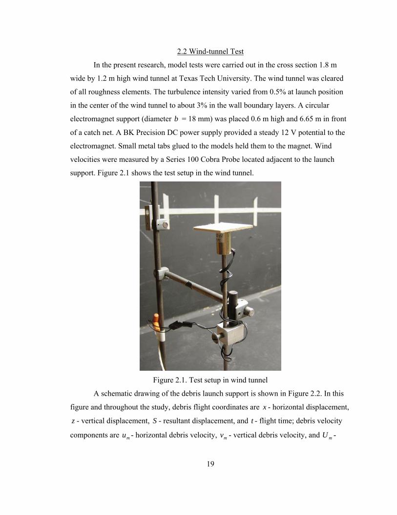
2.2 Wind-tunnel Test

In the present research, model tests were carried out in the cross section 1.8 m

wide by 1.2 m high wind tunnel at Texas Tech University. The wind tunnel was cleared

of all roughness elements. The turbulence intensity varied from 0.5% at launch position

in the center of the wind tunnel to about 3% in the wall boundary layers. A circular

electromagnet support (diameter b = 18 mm) was placed 0.6 m high and 6.65 m in front

of a catch net. A BK Precision DC power supply provided a steady 12 V potential to the

electromagnet. Small metal tabs glued to the models held them to the magnet. Wind

velocities were measured by a Series 100 Cobra Probe located adjacent to the launch

support. Figure 2.1 shows the test setup in the wind tunnel.

Figure 2.1. Test setup in wind tunnel

A schematic drawing of the debris launch support is shown in Figure 2.2. In this

figure and throughout the study, debris flight coordinates are x - horizontal displacement,

z - vertical displacement, S - resultant displacement, and t - flight time; debris velocity

components are mu - horizontal debris velocity, mv - vertical debris velocity, and mU -

20

resultant debris velocity; dimensions of a debris model are h - thickness ( h represents the

edge length of a cube and the diameter of a sphere), B - width perpendicular to flow, D -

length parallel to flow ( D equals to l used in the equations of motion); mρ is debris

density; aρ is air density; U is wind speed at release point; 0α is initial angle of attack.

Figure 2.2. Debris launch support in wind tunnel

An Olympus American Encore MAC PCI version 2.18 digital video camera

(60Hz, 0.0167 second per frame) was used to capture each flight path. Flight time and

coordinates were obtained from the images. Parallax corrections were made to flight

paths assuming that the object stayed largely on the centerline plane of the wind tunnel.

The correction expression for horizontal displacement was obtained by fitting a plot of

the true horizontal distance versus the camera’s x-coordinate; the expression of the

vertical distortion was obtained by fitting a plot of the true vertical distortion versus the

camera’s x-coordinate. The horizontal and the vertical displacements were calculated

from:

1158.00474.10415.00105.0 23 −+−= ccc xxxx (2.1)

0029.00238.00012.00004.0 23 −+−+= cccc xxxzz (2.2)

where cx is the camera’s x-coordinate and cz is the camera’s z-coordinate. Flight

velocity components are then obtained from the corrected displacements.

debris model, ρm,

α0

electromagnet

h

D

bWind, U, ρa

B - perpendicular to flow

x

z

um vm

Um

debris velocities

21

Model characteristics and wind speeds for a given debris type were designed to

provide a range of debris side ratio, support condition, and the Tachikawa parameter K .

The equations of motion (Eqs.1.13-1.15) involve not only the aerodynamic coefficients

( DC , LC , and MC ), but also three non-dimensional parameters mhgUK ρρ 2/2a= ,

mIml /2=∆ , and glUFr /= . In the case of plates or ‘2 by 4’ rectangular cylinders,

∆ =12, and Fr are not directly involved in equations of motion in horizontal and vertical

directions (Eqs. 1.13 and 1.14) and was found to weakly influence debris trajectory

(Holmes et al., 2004), or in the case of compact debris, MC = LC = 0, K becomes the only

significant parameter greatly influencing debris flight for a given debris shape.

The models used in the present research were twenty-two 2D plates, eleven 3D

cubes and spheres, and eight 1D rods at wind speeds ranging from 4.5 m/s to 26 m/s.

Debris materials included various types of wood, plastic, and aluminum, so as to provide

a wide variety of densities. The details of plate models are presented in Table 2.1. Square

and rectangular plates used ranged in weight from 1.1 to 31.7 grams and in side length

from 26 to 150 mm. Table 2.2 presents the wind speeds used for each plate model. The

K values of plates ranged from 2.2 to 32. Cubes and spheres ranging widely in size and

weight were used; the model details are presented in Tables 2.3 and 2.4. The wind speeds

used for each of cubes and spheres were 14.2, 18, 21.8, and 26.8 m/s. The K values of

cubes and spheres ranged from 0.6 to 7.5. The K values of 3D debris are limited, due to

the relatively large characteristic dimension h which requires a very high wind speed to

obtain a high value of K . The details of the ‘2 by 4’ 1D models are presented in Table

2.5; the wind speeds for each of those models were 12, 16, and 25 m/s. The K values of

rods ranged from 3.8 to 27.7.

Three trials were conducted for each model at each wind speed at the initial angle

of attack 0α = 00. In order to investigate the effects of initial angle of attack on debris

trajectory, plates #8, #15, and #21 were also tested at 0α = 150, 450, 900, and 1350, and all

rods were also tested at 0α = 150 and 450. Each model supported at its center was tested.

22

Plate #3 supported at its corner and edge was also tested to investigate the influence of

initial support situation.

Table 2.1. 2D-plate models used in free flight tests in wind tunnel

Plate No. Material Size ( B x D x h )

(mm x mm x mm) Mass

(gram) BD / BDh / (%)

Bb / (%)

#1 basswood 26 x 26 x 9 3.8 1.00 34.62 69.3 #2 balsa 40 x 40 x 1.5 1.1 1.00 3.75 45.0 #3 plastic 42 x 42 x 2 5.1 1.00 4.76 42.9 #4 balsa 50 x 50 x 3 2.1 1.00 6.00 36.0 #5 plywood 50 x 50 x 6 11.1 1.00 12.00 36.0 #6 balsa 55 x 55 x 3 2.6 1.00 5.45 32.7 #7 balsa 75 x 75 x 3 3.2 1.00 4.00 24.0 #8 plywood 75 x 75 x 3 12.3 1.00 4.00 24.0 #9 plywood 75 x 75 x 6 22.3 1.00 8.00 24.0 #10 basswood 75 x 75 x 9 24.8 1.00 12.00 24.0 #11 basswood 76 x 76 x 1.5 5.0 1.00 1.97 23.7 #12 aluminium 76 x 76 x 1.5 25.2 1.00 1.97 23.7 #13 floppy disc 90 x 90 x 2.5 15.0 1.00 2.78 20.0 #14 basswood 150 x 50 x 9 31.7 0.33 10.39 12.0 #15 plastic 120 x 50 x 1 10.5 0.42 1.29 15.0 #16 balsa 126 x 56 x 4.5 4.0 0.44 5.36 14.3 #17 basswood 126 x 56 x 4.5 5.7 0.44 5.36 14.3 #18 plywood 120 x 75 x 3 19.0 0.63 3.16 15.0 #19 plywood 75 x 120 x 3 19.0 1.60 3.16 24.0 #20 balsa 56 x 126 x 4.5 4.0 2.25 5.36 32.1 #21 plastic 50 x 120 x 1 10.5 2.40 1.29 36.0 #22 basswood 50 x 150 x 9 31.7 3.00 10.39 36.0

23

Table 2.2. Wind speeds in free flight tests of plate models in wind tunnel

Plate No. Wind speed U (m/s)

#1 17.9 20.4 20.8 22.7 25.5 26 #2 5.6 6.1 7.4 7.9 8.5 9.7 10.3 12.5 14.8 16.7 17.8 #3 10.3 11.3 13.3 14 14.6 14.8 15.4 15.6 17.3 18.8 19.8 21 22 23.1 24.3 #4 6.5 7.4 7.9 8.5 9.7 10.2 10.3 11.3 13.5 14.6 16.5 17.8 20.7 21.5 22 #5 13.2 15.6 16.4 18.1 19.3 21.4 23.1 24.8 25.6 #6 6 6.5 7.9 8.2 10 10.3 11.3 13.3 14 15.1 16.1 17.3 #7 4.5 4.8 5.2 5.6 6.1 6.8 7.4 8.3 9.7 10.2 11.3 12.5 13.3 13.6 #8 9.1 10.9 11.6 12.5 13.5 15.4 16.4 17.4 18.1 19.3 19.8 20.1 20.9 21.5 #9 12.5 14.6 15.6 17.3 18.1 20.1 22 23.5 24.3 25.6 #10 13.2 15.6 16.4 18.1 19.3 21.4 23.1 24.8 25.6 #11 5.2 5.6 6.5 6.8 7.4 7.9 8.5 9.7 10.2 11.3 13.6 14.8 15.9 16.5 #12 17.3 17.9 18.7 18.8 19.8 21 22 23 23.1 24 #13 9.7 10 12 14 15.1 15.4 18.1 18.8 19.9 #14 16.4 18.5 21 22.7 24 25 #15 7.9 8 9.3 9.6 11.3 12 13.3 14.6 15.1 15.2 15.6 17.3 20 #16 5.8 6.5 8.3 9.2 9.7 10.2 11 12 12.6 13.5 14 #17 5.8 6.5 8.3 9.2 11 12.6 13.5 #18 9.6 10.3 10.7 12.2 12.7 13.5 13.7 15 15.2 16 16.4 #19 9.1 10.9 11.6 12.5 13.6 14.6 16.1 17 17.3 17.7 18.9 19.3 19.8 20.9 21.4 #20 5.8 6.5 8.3 11 12.6 13.5 14.6 16 16.5 17.1 17.9 #21 7.9 11.2 11.3 12 13.2 14.6 15.2 15.6 17.3 18.9 19.2 19.9 21 22 23.1 #22 12.5 15.2 16.1 17.7 18.9 20.9 22.3 22.7 24.2 25.1

Table 2.3. 3D-cube models used in free flight tests in wind tunnel

Cube No. Material Size ( h )

(mm) Mass

(gram) hb /

(%) c1 pine 12 2.0 150 c2 balsa 14 1.3 129 c3 balsa 19 2.0 94.7 c4 pine 19 5.4 94.7 c5 maple 31 21.1 58.1 c6 balsa 38 8.6 47.4

24

Table 2.4. 3D-sphere models used in free flight tests in wind tunnel

Sphere No. Material Size ( h )

(mm) Mass

(gram) hb /

(%) s1 pine 19.1 3.6 94.2 s2 pine 24.9 8.1 72.3 s3 pine 31.8 12.2 56.6 s4 pine 50.1 47.5 35.9 s5 hollow hardboard 65.9 17.8 27.3

Table 2.5. 1D-rod models used in free flight tests in wind tunnel

Rod No. Material Size ( B x D x h )

(mm x mm x mm) Mass

(gram) BD / BDh / (%)

Bb / (%)

r1 pine 12.7 x 381 x 6.4 17.9 30.0 9.2 115 r2 balsa 12.7 x 381 x 6.4 6.0 30.0 9.2 115 r3 pine 381 x12.7 x 6.4 17.9 0.03 9.2 4.72 r4 balsa 381 x12.7 x 6.4 6.0 0.03 9.2 4.72 r5 balsa 12.7 x 330.2 x 6.4 5.5 26.0 9.8 115 r6 balsa 330.2 x12.7 x 6.4 5.5 0.04 9.8 5.45 r7 plywood 12.7 x 330.2 x 6.4 9.8 26.0 9.8 115 r8 plywood 330.2 x12.7 x 6.4 9.8 0.04 9.8 5.45

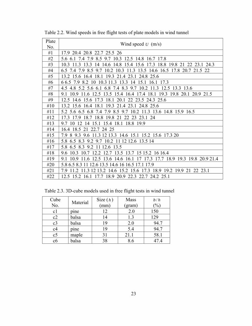
2.3 Full-scale Experiment

Full-scale experiments were conducted with a C-130 Hercules aircraft to generate

strong winds at the west runway of Lubbock Reese Technology Center. The site is

characterized as ASCE exposure category C (the surrounding terrain is open grasslands

and agricultural fields for approximately 1 mile in all directions). Previous experiments

demonstrated that the propeller wash of a C-130 aircraft is suitable for use as a source of

extreme winds (Letchford, 2000). Table 2.6 shows details of the tested full-scale debris

which mainly consisted of rectangular 4 ft x 8 ft plates ranging in weight from 15 to 45

kg, with K ranged from 1.8 to 6.8. The debris plates were launched from a 1 m high

table in the field. Wind velocities were measured by an RM Young propeller/vane

anemometer located 1 m high and 1 m upstream of the launch table. Figure 2.3 shows the

experimental field and the flight of a sheet. The same video camera used in the wind-

25

tunnel tests was employed here. The notation system is the same as that used in the wind-

tunnel tests.

Figure 2.3. Full-scale experiment of debris trajectory

26

Table 2.6. Details of full-scale debris

Plate No. Material Size ( B x D x h )

(m x m x m) Mass (kg) BD / BDh /

(%)

Wind speed (m/s)

C2 3/8" MDF 2.46 x 1.24 x 0.0095 22.5 0.50 5.44 24.1 D1 2.44 x 1.22 x 0.025 15.0 0.50 14.5 24.1 D2

Tempered Hardboard + Styrofoam

2.44 x 1.22 x 0.025 19.3 0.50 14.5 21.8

E1 2.46 x 1.24 x 0.019 43.2 0.50 10.9 26.4 E2 2.46 x 1.24 x 0.019 42.5 0.50 10.9 24.4 E3 2.46 x 1.24 x 0.019 43.7 0.50 10.9 20.3 E4

3/4 " MDF

1.24 x 2.46 x 0.019 46.2 2.00 10.9 21.5

2.4 Data Analysis and Interpretation

Data analysis procedure comprised three parts: exporting raw data from each

digital camera file, calculating flight variables for each trial, and conducting

dimensionless analysis to collapse the data.

The flight path was recorded as an image file. There were three steps to obtain the

raw data. First, calibrating the camera x-coordinate with a reference distance; second,

locating the object positions on the image at each time interval ∆t ≈ 0.083 secs (about

five frames) to obtain the coordinates; and third, exporting the raw data (including

coordinates and time intervals) to a WordPad file which was then imported into an Excel

spreadsheet.

The data was analyzed in Excel to determine the displacements and velocities at

each time step. Parallax corrections were undertaken at this stage to obtain the horizontal

and vertical displacements from the camera coordinates via Equations 2.1 and 2.2.

Horizontal, vertical, and resultant velocities were calculated from the displacements.

Time nominally started at the moment of release.

Figures 2.4, 2.5, and 2.6 are examples of displacement analyses of one model

(plate #8) at three wind speeds. As shown in Figure 2.4, at a relatively low wind speed,

three trials showed quite similar trajectories of the debris when falling. This similarity is

also apparent at high wind speeds when the models fly up (Figure 2.5). Figure 2.6 shows

that, at a critical wind speed, trial results may show some difference. However, this

27

difference is predominately in the vertical direction, in which the displacement scale is

much lower than that of the horizontal direction. Horizontal displacements are quite

consistent for each trial of a model at a given wind speed.

Figures 2.7, 2.8, and 2.9 are examples of velocity analyses of one model (plate

#8). Figure 2.7 shows the calculation of horizontal ( mu ) and resultant ( mU ) velocities of

one trial by two methods. The first method used discrete displacements to calculate

velocities: txum ∆∆= / ( tSU m ∆∆= / ), with t∆ ≈ 0.083 secs. The second method

involved fitting the best fit polynomials to the displacements and derivation to obtain

velocities: dtdxum /= ( dtdSU m /= ), in which )(tx and )(tS are fitted polynomial

functions (R-squared values over 0.99). The second method results in smooth graphs.

Although the results from the second method do not reflect the real debris velocity very

well at the beginning of flight, the two methods yield similar results for the portions of

high debris flight speed. At low wind speeds, the resultant velocity of a model is higher

than its horizontal velocity due to the relative importance of its vertical velocity

component (Figure 2.7a), while at higher wind speeds, the resultant and horizontal

velocities are much closer in agreement (Figure 2.7b). This difference in velocities

reflects the influence of the lift force on the debris. The closer the two curves, the smaller

is vm, indicating the greater the lift force sustaining the debris flight and counteracting the

effects of gravity.

Figure 2.8 and Figure 2.9 show the horizontal and vertical velocities of a plate,

respectively. Horizontal and resultant debris velocities used in the following discussion

were obtained by averaging the results from the two calculation methods. The vertical

speed was calculated from the incremental vertical displacement (vm=∆z/∆t).

28

0

1

2

3

4

5

6

0 0.2 0.4 0.6 0.8

t (sec)

x (m

)

Trial 1Trial 2Trial 3

-0.6

-0.4

-0.2

0

0.2

0.4

0.6

0 0.1 0.2 0.3 0.4 0.5 0.6 0.7

t (sec)

z (m

)


-0.6

-0.4

-0.2

0

0.2

0.4

0.6

0 0.5 1 1.5 2

x (m)

z (m

)


Figure 2.4. Analysis of debris trajectories (Plate #8, U=9.1 m/s, α0 = 00)

29

0

1

2

3

4

5

6

0 0.1 0.2 0.3 0.4 0.5

t (sec)

x (m

)


0

0.1

0.2

0.3

0.4

0.5

0.6

0 0.1 0.2 0.3 0.4 0.5

t (sec)

z (m

)


0

0.1

0.2

0.3

0.4

0.5

0.6

0 1 2 3 4 5

x (m)

z (m

)



30

0

1

2

3

4

5

6

0 0.1 0.2 0.3 0.4 0.5 0.6

t (sec)

x (m

)


0

0.1

0.2

0.3

0.4

0.5

0.6

0 0.1 0.2 0.3 0.4 0.5 0.6

t (sec)

z (m

)


0

0.1

0.2

0.3

0.4

0.5

0.6

0 1 2 3 4 5

x (m)

z (m

)



31

0

0.2

0.4

0.6

0.8

1

0 0.1 0.2 0.3 0.4 0.5 0.6

Time (sec)

plat

e sp

eed

/ win

d sp

eed

UmUm (ds/dt)

umum (dx/dt)

(a) Plate #8, U=9.1 m/s, α0 = 00

0

0.2

0.4

0.6

0.8

1

0 0.1 0.2 0.3 0.4 0.5 0.6

Time (sec)

plat

e sp

eed

/ win

d sp

eed

Um

Um (ds/dt)

um

um (dx/dt)

(b) Plate #8, U=16.4 m/s, α0 = 00

Figure 2.7. Calculation of debris horizontal and resultant velocities

tsU m ∆∆= /dtdsU m /=tsum ∆∆= /

dtdsum /=


dtdsum /=

32

0

0.2

0.4

0.6

0.8

1

0 0.2 0.4 0.6 0.8

t (sec)

um/U


0

0.2

0.4

0.6

0.8

1

0 0.5 1 1.5 2

x (m)

um/U


Figure 2.8. Analysis of debris horizontal velocity (Plate #8, U=9.1 m/s, α0 = 00)

33

-0.4

-0.2

0

0.2

0 0.2 0.4 0.6 0.8

t (sec)

vm/U


-0.4

-0.2

0

0.2

-0.6 -0.4 -0.2 0 0.2

z (m)

vm/U


Figure 2.9. Analysis of debris vertical velocity (Plate #8, U=9.1 m/s, α0 = 00)

34

Figures 2.4, 2.8, and 2.9 presented the relationships of actual flight variables (time,

displacement, and velocity) of the trajectory of a debris model (plate #8) at a given wind

speed (9.1 m/s). In order to translate the experimental results to full-scale, the data was

non-dimensionalized: time - Ugtt /= , horizontal displacement - 2/Ugxx = , vertical

displacement - 2/Ugzz = , horizontal velocity - Uuu m /= , and vertical velocity -

Uvv m= . This scheme was based on the dimensionless equations of motion (Eqs. 1.13,

1.14, and 1.15) developed by Tachikawa (1983). In this scheme, Figures 2.4, 2.8, and 2.9

become Figures 2.10, 2.11, and 2.12, which present the displacements ( x ~t , z ~ t , and

z ~ x ), horizontal velocity (u ~t and u ~ x ), and vertical velocity ( v ~ t and v ~ z ),

respectively. All experimental trajectories were analyzed in this manner and are presented

in Chapter 3.

It should be noted that the non-dimensional relationships presented in Figures

2.10-2.12 cannot determine debris flight aerodynamics nor be directly applied to full-

scale design, because, for the same type of debris, the relationships change with the value

of K . In addition to the non-dimensional variables, the value of K was also calculated

for each test. This non-dimensional parameter K is then combined with the non-

dimensional variables so that the flight aerodynamic characteristics of debris can be used

for full-scale design. The results and applications are discussed in Chapter 3.

35

0

0.2

0.4

0.6

0 0.5 1 1.5


-0.2

-0.1

0

0.1

0 0.5 1 1.5


-0.2

-0.1

0

0.1

0 0.2 0.4 0.6


Figure 2.10. Non-dimensional analysis of debris displacements

(Plate #8, K =2.1, Fr =8.9 x 10-3, α0 = 00)

Ugtt =

2Ugxx =

2Ugzz =

2Ugzz =

Ugtt =

2Ugxx =

36

0

0.2

0.4

0.6

0.8

1

0 0.5 1 1.5


0

0.2

0.4

0.6

0.8

1

0 0.2 0.4 0.6


Figure 2.11. Non-dimensional analysis of debris horizontal velocity

(Plate #8, K =2.1, Fr =8.9 x 10-3, α0 = 00)

Ugtt /= Ugtt /=

2/Ugxx =

Uu

u m=

Uu

u m=

37

-0.4

-0.2

0

0.2

0 0.5 1 1.5


-0.4

-0.2

0

0.2

-0.2 -0.1 0 0.1


Figure 2.12. Non-dimensional analysis of debris vertical velocity

(Plate #8, K =2.1, Fr =8.9 x 10-3, α0 = 00)

Ugtt /=

2/Ugzz =

Uvv m=

Uvv m=

38

CHAPTER III

SIMULATION RESULTS AND DISCUSSION

3.1 Introduction

Wind-tunnel simulations of the trajectories of twenty-two 2D plates, six cubes,

five spheres, and eleven rods, at wind speeds ranging from 4.5 m/s to 26 m/s in uniform

flows were conducted. Although debris trajectories presented great variation, it was

found that a pattern emerged for the horizontal trajectory of debris. Non-dimensional

analysis collapsed the horizontal trajectories of debris for an extensive set of model tests,

and the results were comparable to full-scale results. Experimental expressions have been

developed and can be used in debris impact criteria. The results of plates have been

presented in a previous paper (Lin et al., 2005).

Section 3.2 presents debris trajectories from wind-tunnel tests. The main

parameters determining debris trajectories fall into three categories: wind field, debris

properties, and debris initial support. The effects on the debris trajectory of the

parameters were investigated.

Section 3.3 presents debris horizontal trajectories, using the non-dimensional

scheme developed by Tachikawa (1983). Experimental expressions of horizontal flight

speed as a function of flight distance, and flight distance as a function of sustaining time

were established, based on both wind-tunnel test results and theoretical equations of

debris motion.

Comparisons of wind-tunnel test with full-scale test results are made in Section

3.4. Trajectories of full-scale sheets are comparable with those of model plates, especially

in the horizontal dimension.

As application examples, Section 3.5 presents the horizontal trajectories of

representative debris items which are usually used in debris impact tests. Good agreement

of experiment solutions and numerical solutions was obtained. The empirical method can

be used to establish rational debris impact test criteria.

39

3.2 Characteristics of Debris Trajectory

The experimental results indicate that, for certain debris shape, debris trajectory

(T ) is a function of at least nine parameters: wind speed (U ), air density ( aρ ), plate

dimensions ( B , D , and h ), plate density ( mρ ), support dimension (b ), support position

( s , e.g., center, corner, or edge), and initial angle of attack ( 0α ), and can be expressed as:

),,,,,,,,( 0αρρ sbDBhUfT ma= (3.1)

where U and aρ characterize the wind field, h , B , D , and mρ are the debris

characteristics, and b , s , and 0α describe the debris initial support configuration.

The variations of two-dimensional plate trajectories within these parameters were

investigated. Figure 3.1 shows the trajectories of plate #8 at wind speeds ranging from

8.5 m/s to 20.8 m/s. The higher the wind speed, the higher the flight path. Figure 3.2

shows the effect of plate density on plate trajectories. With the same geometric

dimensions but different material, plate #7 ( 0057.0/ =ma ρρ ) flew higher than plate #8

( 0015.0/ =ma ρρ ), at the same wind speed. Figure 3.3 shows the effect of plate

dimension h on plate trajectories. Comparison of trajectories of three square plates

( BDh / =2.8-8.0%) with similar b/B values (20 – 24%) clearly show that the lift force

increases with decreasing BDh / , and overcomes gravity to accelerate the plate into the

air.

The effects of U , aρ , mρ , and h on debris trajectories can be presented using the

non-dimensional parameter Tachikawa mhgUK ρρ 2/2a= (the ratio of aerodynamic

force to gravity force). Reducing the parameters, Equation (3.1) can be rewritten as:

),,/,/,( 0 sBbBDKfT α= . (3.2)

Figure 3.4 shows the trajectories of four square plates with different values of K

while holding the values of the other parameters in Equation (3.2) constant. As expected,

plate trajectories rise as K increases.

40

-0.6

-0.4

-0.2

0

0.2

0.4

0.6

0 1 2 3 4 5 6

Horizontal displacement (m)

Vert

ical

dis

plac

emen

t (m

) Vw=8.5Vw=10Vw=10.8Vw=11.9Vw=13.9Vw=15.3Vw=16.3Vw=18.0Vw=20.8

Figure 3.1. Plate trajectories at different wind speeds

(Plate #8, ma ρρ / =0.0015, BD / =1, BDh / =4%, Bb / =24%, 0α =00, s -center)

-0.6

-0.4

-0.2

0

0.2

0.4

0.6

0 1 2 3 4 5 6Horizontal displacement (m)

Vert

ical

dis

plac

emen

t (m

)

# 7

# 8

Figure 3.2. Plate trajectories affected by debris density

(U = 12.5m/s, BD / =1, BDh / =4%, Bb / =24%, 0α =00, s -center)

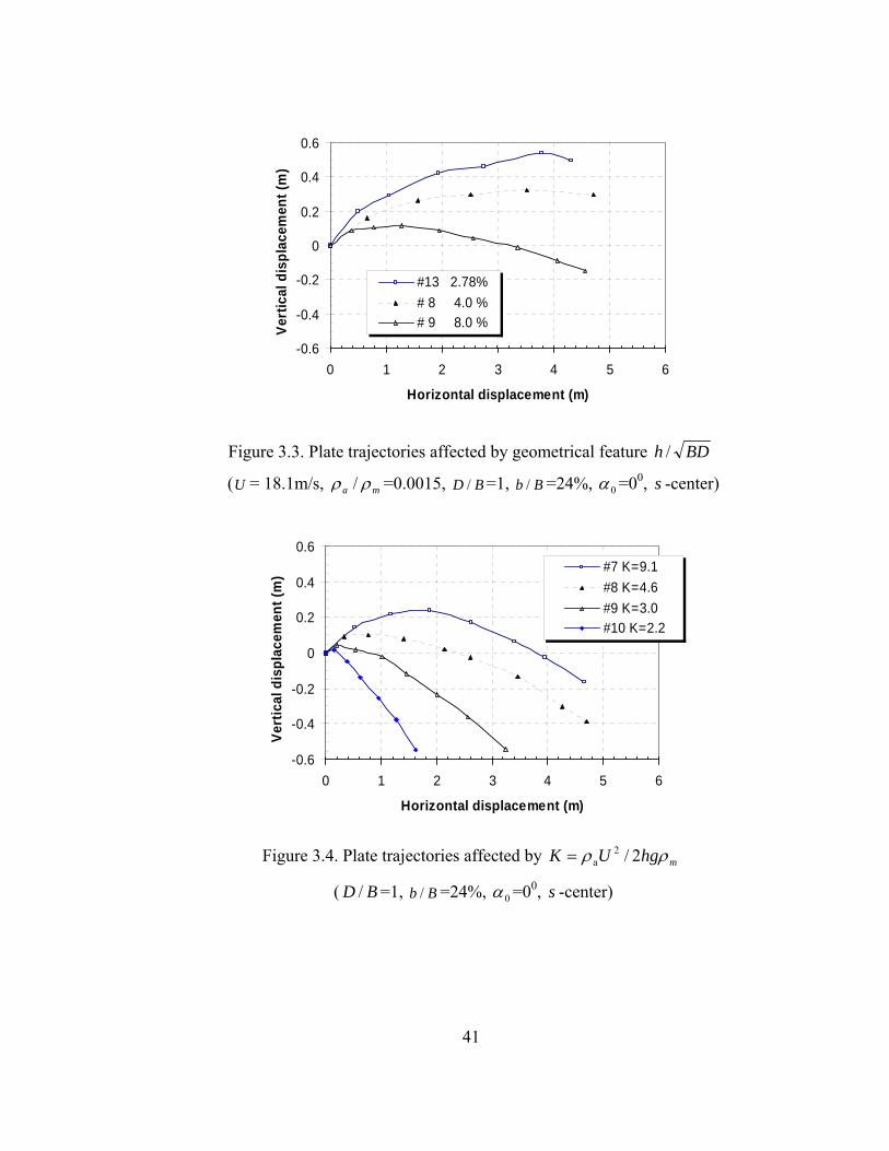
41

-0.6

-0.4

-0.2

0

0.2

0.4

0.6

0 1 2 3 4 5 6


Vert

ical

dis

plac

emen

t (m

)#13 2.78% # 8 4.0 %# 9 8.0 %

Figure 3.3. Plate trajectories affected by geometrical feature BDh /

(U = 18.1m/s, ma ρρ / =0.0015, BD / =1, Bb / =24%, 0α =00, s -center)

-0.6

-0.4

-0.2

0

0.2

0.4

0.6

0 1 2 3 4 5 6


Vert

ical

dis

plac

emen

t (m

) #7 K=9.1#8 K=4.6#9 K=3.0#10 K=2.2

Figure 3.4. Plate trajectories affected by mhgUK ρρ 2/2a=

( BD / =1, Bb / =24%, 0α =00, s -center)

42

Side ratio ( BD / ), another plate geometrical feature, also greatly affects the

trajectory. As shown in Figure 3.5, given the same K value and holding the other

parameters constant, the smaller the side ratio, the higher the plate flew. The trajectory

variation is greater when BD / > 1 than it is when BD / <1.

-0.6

-0.4

-0.2

0

0.2

0.4

0.6

0 1 2 3 4 5 6


Vert

ical

dis

plac

emen

t (m

)#6 D/B=1

#20 D/B=2.25

( K =6.7, Bb / =33%, 0α =00, s -center, 1/ ≥BD )

-0.6

-0.4

-0.2

0

0.2

0.4

0.6

0 1 2 3 4 5 6


Vert

ical

dis

plac

emen

t (m

)

#15 D/B=0.42

#18 D/B=0.63

#13 D/B=1

( K =6.7, Bb / =15-20%, 0α =00, s -center, 1/ ≤BD )

Figure 3.5. Plate trajectories affected by geometrical feature BD /

43

In addition to K and BD / , three initial situation factors greatly affected plate

trajectories: b , s , and 0α . Figure 3.6 presents the influence of the support dimension.

Given the same K values, the trajectories of plate #10 ( Bb / = 24%) and plate #1 ( Bb / =

69%) show that the smaller the ratio of support diameter to plate width ( Bb / ), the larger

the initial lift force, increasing the flight altitude. Figure 3.7 shows the trajectories of

plate #3 supported at the center, corner, and edge, respectively, at a given wind speed.

When support was at the center of the plate, the lift force developed on the front half of

the plate was largely unaffected by the support; however, when support was at the middle

of the plate’s leading edge, gross disturbance to the flow occurred at the critical lift

generation position, lowering the altitude of the plate’s flight. Support at a corner of the

plate resulted in a combination of these two effects.

-0.6

-0.4

-0.2

0

0.2

0.4

0.6

0 1 2 3 4 5 6


Vert

ical

dis

plac

emen

t (m

)

#10 b/B=24%

#1 b/B=69%

Figure 3.6. Plate trajectories affected by relative support dimension Bb /

( K =7.6, BD / =1, 0α =00, s -center)

44

-0.6

-0.4

-0.2

0

0.2

0.4

0.6

0 1 2 3 4 5 6


Vert

ical

dis

plac

emen

t (m

) #3 center#3 corner#3 edge

Figure 3.7. Plate trajectories affected by support place s

( K =3.37, BD / =1, Bb / =43%, 0α =00)

Video records showed that the trajectory pattern of a plate depends mainly on its

mode of motion, which in turn is closely related to the initial angle of attack ( 0α ).

Figures 3.8, 3.9, and 3.10 show, with different α0, at relatively low and high values of K ,

the trajectories of square plate #8, rectangular plate #15 ( BD / =0.42), and rectangular

plate #21 ( BD / =2.4), respectively. Tachikawa (1983) defined three flight modes for

plates: auto-rotating, intermediate, and translatory. In the present study, plates generally

entered into clockwise auto-rotation and ‘flew up’ over a long distance at 0α =00 and

0α =150. At 0α =450 and 0α =900, the intermediate mode changed from clockwise to

counter-clockwise rotation at initial stages of flight and then to translatory mode at 450 to

horizontal until hitting the ground. At 0α =1350, at relatively low wind speed, one or two

counter-clockwise rotations were followed by translatory mode, also at 450 to ground

(Figures 3.8a, 3.9a, and 3.10a). However, as wind speed increases, the translatory mode

of plates may change to clockwise rotation and the plates fly up (Figures 3.8b, 3.9b, and

3.10b). At 0α =1650, plates entered into counter-clockwise auto-rotation. It was noted that

at 0α =150, plate #15 ( BD / =0.42) had low flight paths at both wind speeds (Figure 3.9).

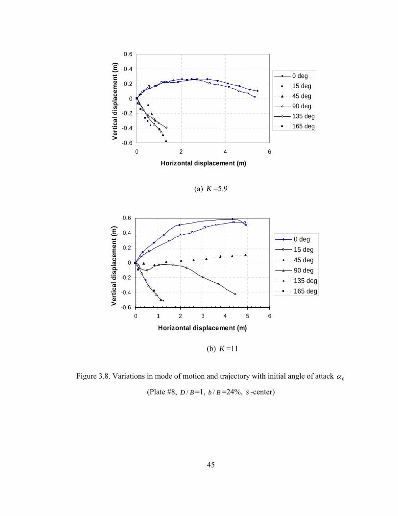
45

-0.6

-0.4

-0.2

0

0.2

0.4

0.6

0 2 4 6


Vert

ical

dis

plac

emen

t (m

)

0 deg15 deg45 deg90 deg135 deg165 deg

(a) K =5.9

-0.6

-0.4

-0.2

0

0.2

0.4

0.6

0 1 2 3 4 5 6


Vert

ical

dis

plac

emen

t (m

)


(b) K =11

Figure 3.8. Variations in mode of motion and trajectory with initial angle of attack 0α

(Plate #8, BD / =1, Bb / =24%, s -center)

46

-0.6

-0.4

-0.2

0

0.2

0.4

0.6

0 1 2 3 4 5


Vert

ical

dis

plac

emen

t (m

)


(a) K =4.5

-0.6

-0.4

-0.2

0

0.2

0.4

0.6

0 1 2 3 4 5


Vert

ical

dis

plac

emen

t (m

)


(b) K =12.5


(Plate #15, BD / =0.42, Bb / =15%, s -center)

47

-0.6

-0.4

-0.2

0

0.2

0.4

0.6

0 1 2 3 4


Vert

ical

dis

plac

emen

t (m

)


(a) K =4.5

-0.6

-0.4

-0.2

0

0.2

0.4

0.6

0 1 2 3 4 5


Vert

ical

dis

plac

emen

t (m

)


(b) K =11.2


(Plate #21, BD / =2.4, Bb / =36%, s -center)

48

Although plate trajectories showed great variations in the vertical direction within

each of the five parameters in Equation (3.2), the horizontal component of the plate

trajectories presented certain patterns. Figures 3.11-3.21 show the effect of each

parameter on horizontal plate trajectories, in terms of horizontal velocity versus

horizontal displacement, and horizontal displacement versus time.

It was seen in Figure 3.4 that plate trajectories rise as K increases. K also greatly

affects horizontal components of plate trajectories. Figure 3.11 shows that horizontal

speed (at a given horizontal displacement) increases with K , as does the horizontal

displacement (at a given time).

Plate trajectories rise as side ratio ( BD / ) decreases (Fig.3.5); however, BD /

appears to only slightly affect plate horizontal trajectory. In Figure 3.12, horizontal

velocities (at a given horizontal distance) of plate #6 ( BD / =1) and plate #20 ( BD / =2.25)

are practically identical. The horizontal displacement (at a given time) of plate #20 is

slightly less than that of plate #6. When ≤BD / 1, BD / has little influence on either

velocity or horizontal displacement, as shown in Figure 3.13. This indicates that given the

same value of K , square and rectangular plates present similar flight trajectories in the

horizontal direction, even though they have different aerodynamic coefficients. This

feature is further illustrated in Section 3.3 by comparing the horizontal trajectories of all

twenty-two plates with a range of K values.

The effects of initial situation on the horizontal plate trajectories are also very

small. Figure 3.14 shows that there is very little influence of the relative support

dimension ( Bb / ) on horizontal plate trajectories with the same K . Figure 3.15 shows

that plate 3 supported at the center, corner, and edge, respectively, followed an almost

identical horizontal trajectory. The initial angle of attack ( 0α ) has relatively little effect.

Although the mode of motion, which is closely related to 0α , greatly affects the plate

trajectories in the vertical direction (Figs. 3.8-3.10), the corresponding horizontal

trajectories are almost independent of 0α (Figs. 3.16-3.21), except that plate #15 showed

lower speeds at 0α =150, at the low wind speed (Fig. 3.18). Therefore, initial situation

greatly influences the vertical trajectory of plates, but not the horizontal trajectory.

49

0

0.2

0.4

0.6

0.8

1

0 1 2 3 4 5 6


Hor

izon

tal s

peed

/ W

ind

spee

d#7 K=9.1#8 K=4.6#9 K=3.0#10 K=2.2

0

1

2

3

4

5

0 0.2 0.4 0.6 0.8 1 1.2

Time (sec)

Hor

izon

tal d

ispl

acem

ent (

m) #7 K=9.1

#8 K=4.6#9 K=3.0#10 K=2.2

Figure 3.11. Horizontal plate trajectories affected by mhgUK ρρ 2/2a=

( BD / =1, Bb / =24%, 0α =00, s -center)

50

0

0.2

0.4

0.6

0.8

1

0 1 2 3 4 5 6


Hor

izon

tal s

peed

/ W

ind

spee

d#6 D/B=1

#20 D/B=2.25

0

1

2

3

4

5

6

0 0.2 0.4 0.6 0.8 1 1.2

Time (sec)

Hor

izon

tal d

ispl

acem

ent (

m)

#6 D/B=1

#20 D/B=2.25

Figure 3.12. Horizontal plate trajectories affected by side ratio ( ≥BD / 1)

( K =6.7, Bb / =33%, 0α =00, s -center)

51

0

0.2

0.4

0.6

0.8

1

0 1 2 3 4 5 6


Hor

izon

tal s

peed

/ W

ind

spee

d#15 D/B=0.42

#18 D/B=0.63

#13 D/B=1

0

1

2

3

4

5

6

0 0.2 0.4 0.6 0.8 1 1.2

Time (sec)

Hor

izon

tal d

ispl

acem

ent (

m)

#15 D/B=0.42

#18 D/B=0.63

#13 D/B=1

Figure 3.13. Horizontal plate trajectories affected by side ratio ( ≤BD / 1)

( K =6.7, Bb / =15-20%, 0α =00, s -center)

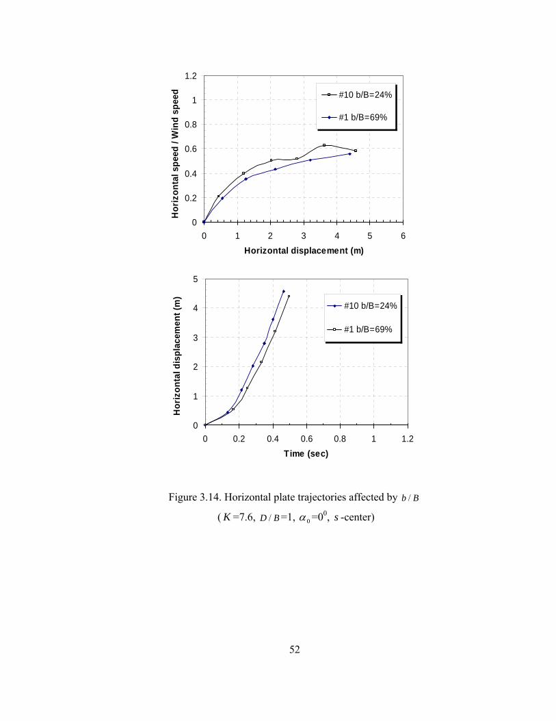
52

0

0.2

0.4

0.6

0.8

1

1.2

0 1 2 3 4 5 6Horizontal displacement (m)

Hor

izon

tal s

peed

/ W

ind

spee

d #10 b/B=24%

#1 b/B=69%

0

1

2

3

4

5

0 0.2 0.4 0.6 0.8 1 1.2Time (sec)

Hor

izon

tal d

ispl

acem

ent (

m)

#10 b/B=24%

#1 b/B=69%

Figure 3.14. Horizontal plate trajectories affected by Bb /

( K =7.6, BD / =1, 0α =00, s -center)

53

0

0.2

0.4

0.6

0.8

1

0 1 2 3 4 5 6


Hor

izon

tal s

peed

/ W

ind

spee

d #3 center#3 corner#3 edge

0

1

2

3

4

5

0 0.2 0.4 0.6 0.8 1 1.2

Time (sec)

Hor

izon

tal d

ispl

acem

ent (

m) #3 center

#3 corner#3 edge

Figure 3.15. Horizontal plate trajectories affected by s

( K =3.37, BD / =1, Bb / =43%, 0α =00)

54

0

0.2

0.4

0.6

0.8

1

0 2 4 6


Hor

izon

tal s

peed

/ Win

d sp

eed


0

1

2

3

4

5

6

0 0.2 0.4 0.6 0.8 1 1.2Time (sec)

Hor

izon

tal d

ispl

acem

ent (

m)


Figure 3.16. Horizontal trajectories affected by initial angle of attack 0α

(Plate #8, BD / =1, K =5.9, Bb / =24%, s -center)

55

0

0.2

0.4

0.6

0.8

1

0 2 4 6Horizontal displacement (m)

Hor

izon

tal s

peed

/ W

ind

spee

d


0

1

2

3

4

5

6

0 0.2 0.4 0.6 0.8 1 1.2Time (sec)

Hor

izon

tal d

ispl

acem

ent (

m)



(Plate #8, BD / =1, K =11, Bb / =24%, s -center)

56

0

0.2

0.4

0.6

0.8

1

0 1 2 3 4 5


Hor

izon

tal s

peed

/ W

ind

spee

d


0

1

2

3

4

5

0 0.2 0.4 0.6 0.8 1 1.2

Time (sec)

Hor

izon

tal d

ispl

acem

ent (

m)



(Plate #15, BD / =0.42, K =4.5, Bb / =15%, s -center)

57

0

0.2

0.4

0.6

0.8

1

0 1 2 3 4 5


Hor

izon

tal s

peed

/ W

ind

spee

d


0

1

2

3

4

5

6

0 0.2 0.4 0.6 0.8 1 1.2

Time (sec)

Hor

izon

tal d

ispl

acem

ent (

m)




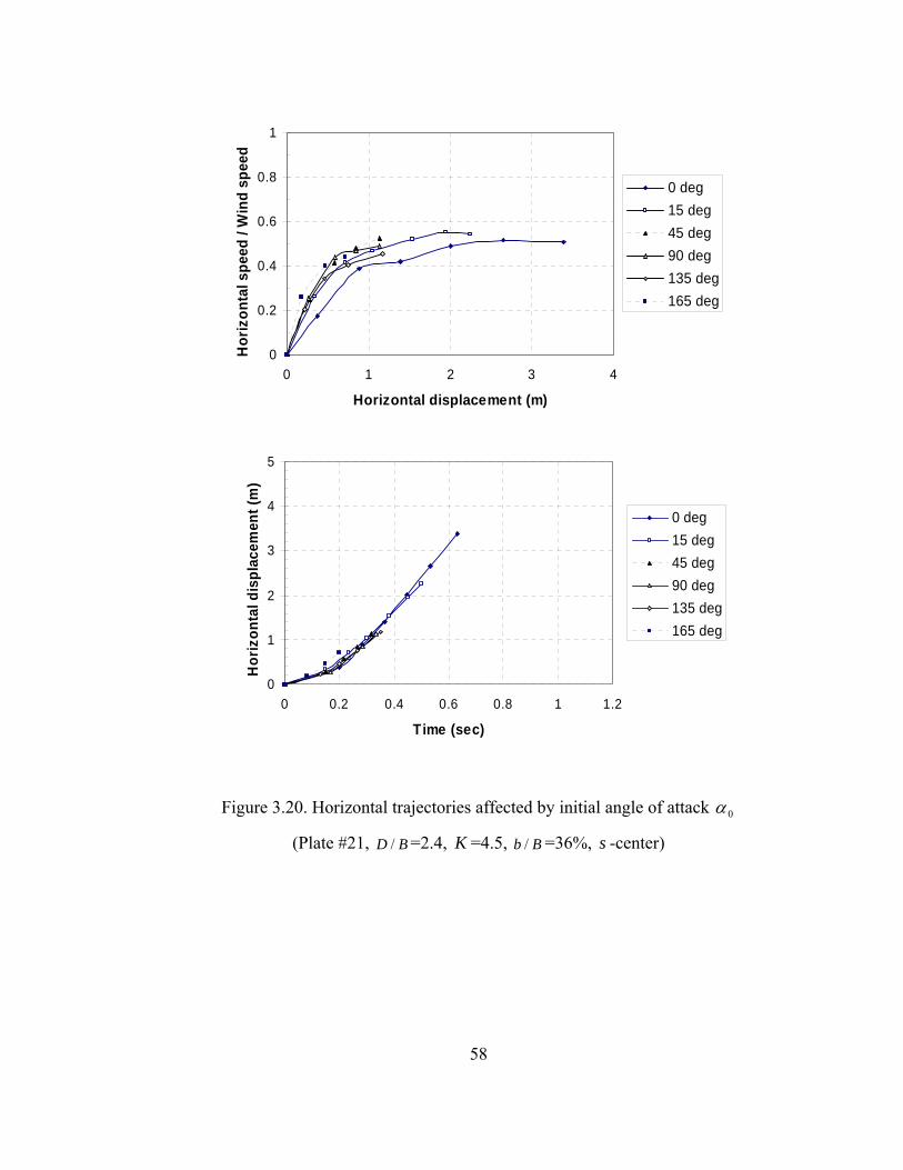
58

0

0.2

0.4

0.6

0.8

1

0 1 2 3 4


Hor

izon

tal s

peed

/ W

ind

spee

d


0

1

2

3

4

5

0 0.2 0.4 0.6 0.8 1 1.2

Time (sec)

Hor

izon

tal d

ispl

acem

ent (

m)




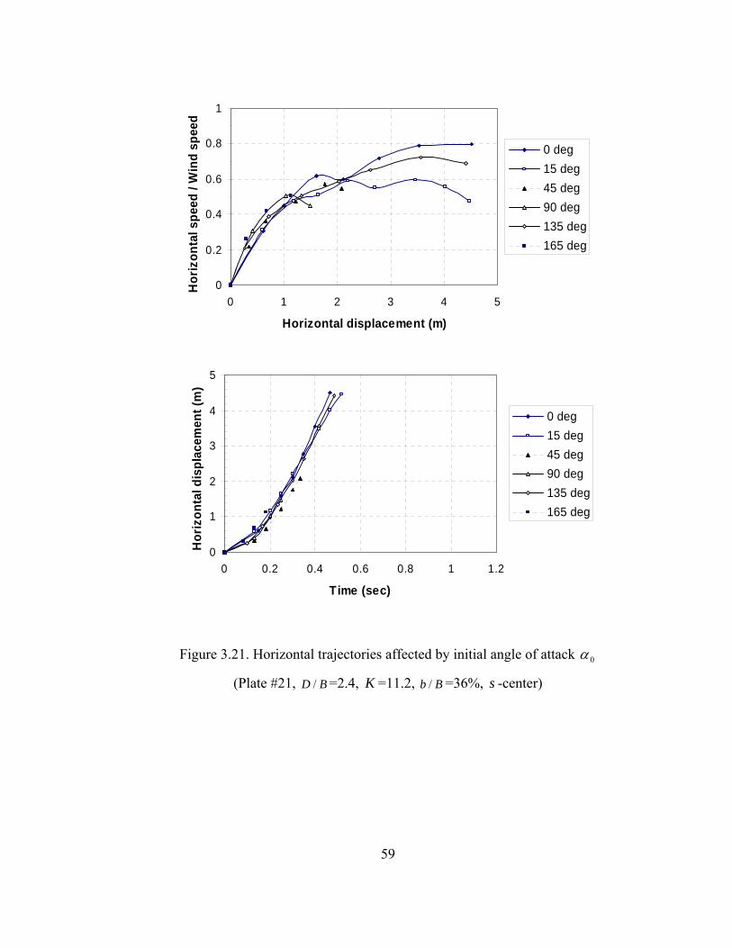
59

0

0.2

0.4

0.6

0.8

1

0 1 2 3 4 5


Hor

izon

tal s

peed

/ W

ind

spee

d


0

1

2

3

4

5

0 0.2 0.4 0.6 0.8 1 1.2

Time (sec)

Hor

izon

tal d

ispl

acem

ent (

m)




60

The investigation of two-dimensional trajectory of 2D plate-like debris was

expanded to 3D compact-like debris and 1D rod-like debris. Since only drag forces were

significant, 3D cubes and spheres traveled relatively short distances in the tests and initial

support situation had little influence on their trajectories, and their horizontal trajectories

presented similar characteristics to those of plates. With drag, lift, and pitching moments,

akin to plates, 1D rods were found to have more variation in the vertical direction than

plates; however, the horizontal component of the rod trajectories presented certain

characteristics comparable to the characteristics of plates.

3.3 Non-dimensional Horizontal Debris Trajectory

The horizontal trajectory of a particular debris type, then, is mainly dependent on

K . Data showed that non-dimensional horizontal trajectories of each debris shape with

different side ratio, in different initial situations, and at a range of wind speeds, collapsed

for each K ( 322 ≤≤ K ). Figures 3.22, 3.23, 3.24, and 3.25 are examples of horizontal

trajectories of plates when K is equal to 2, 4, 6, and 9, respectively. The data show that

non-dimensional horizontal velocity of debris with given K is primarily a function of

non-dimensional horizontal displacement, which is a function of non-dimensional time.

Note that the velocity of rectangular plates with BD / >1 decreases at the end of the

trajectory, due to mean wind speed reducing in boundary layers and due to boundary

layer turbulence close to the wind-tunnel ceiling or floor. This boundary layer turbulence

has scales which may influence the aerodynamic forces acting (Holmes, 2004). The

horizontal displacements of rectangular plates show little difference from those of square

plates, except for a slight decrease when BD / >1.

61

0

0.2

0.4

0.6

0.8

1

1.2

0.0 0.2 0.4 0.6 0.8 1.0

#15 (D/B=0.42) #17 (0.44)#18 (0.63) D/B=1#19 (1.6) #21(2.4)#22 (3.0)

0

0.2

0.4

0.6

0.8

1

0.0 0.2 0.4 0.6 0.8 1.0 1.2 1.4 1.6

#15 (D/B=0.42) #17 (0.44)#18 (0.63) D/B=1#19 (1.6) #21(2.4)#22 (3.0)

Figure 3.22. Non-dimensional plate trajectories in the horizontal direction ( K =2)

2Ugxx =

Ugtt =

Uu

u m=

2Ugxx =

62

0

0.2

0.4

0.6

0.8

1

1.2

0.0 0.2 0.4 0.6 0.8 1.0

#14 (0.33) #15 (D/B=0.42)#16 (0.44) #18 (0.63)D/B=1 #19(1.6)#20 (2.25) #21 (2.4)#22 (3.0)

0

0.2

0.4

0.6

0.8

1

0.0 0.2 0.4 0.6 0.8 1.0 1.2 1.4 1.6

#14 (0.33) #15 (D/B=0.42)#16 (0.44) #18 (0.63)D/B=1 #19(1.6)#20 (2.25) #21 (2.4)#22 (3.0)


2Ugxx =

Ugtt =

Uu

u m=

2Ugxx =

63

0

0.2

0.4

0.6

0.8

1

1.2

0.0 0.2 0.4 0.6 0.8 1.0

#14 (0.33) #15 (D/B=0.42)#17 (0.44) #18 (0.63)D/B=1 #19(1.6)#21 (2.4) #22 (3.0)

0

0.2

0.4

0.6

0.8

1

0.0 0.2 0.4 0.6 0.8 1.0 1.2 1.4 1.6

#14 (0.33) #15 (D/B=0.42)#17 (0.44) #18 (0.63)D/B=1 #19(1.6)#21 (2.4) #22 (3.0)


2Ugxx =

Ugtt =

Uuu m=

2Ugxx =

64

0

0.2

0.4

0.6

0.8

1

1.2

0.0 0.2 0.4 0.6 0.8 1.0

#15 (D/B=0.42) #16 (0.44)

D/B=1 #19(1.6)#21 (2.4)

0

0.2

0.4

0.6

0.8

1

0.0 0.2 0.4 0.6 0.8 1.0 1.2 1.4 1.6

#15 (D/B=0.42) #16 (0.44)D/B=1 #19(1.6)#21 (2.4)


2Ugxx =

Ugtt =

Uuu m=

2Ugxx =

65

Non-dimensional equation of debris motion in the horizontal direction developed

by Tachikawa (Eq. 1.13) is rewritten here:

])1)[(sincos( 222

2

vuCCKtdud

tdxd

LD +−−== ββ (3.3)

where 22)1(

1cosvu

u+−

−=β and

22)1(sin

vuv

+−=β .

Since debris horizontal trajectory is mainly dependent on K , the aerodynamic term

)sincos( ββ LD CC − can be denoted as C , and denote pC , cC , sC , and rC as the

coefficient for plates, cubes, spheres, and rods, respectively. Equation (3.3) becomes:

])1[( 222

2

vuCKtdud

tdxd

+−== . (3.4)

For u , v <<1 (i.e., in the early part of the flight), →βcos 1, →βsin 0, and

KCtdud

tdxd

D→=2

2

. Integrating,

tKCu D= , 2

21 tKCx D= , and xKCu D2= . (3.5)

Baker (2004) suggested similar limiting relationships, but only for compact (3D) objects.

Equations 3.4 and 3.5 indicate that for a certain debris type, u is a function of

xK , and xK is a function of tK . Accordingly, all experimental data are presented in

Figures 3.26, 3.27, and 3.28, for 2D, 3D, and 1D debris, respectively. Figure 3.26 shows

u as a function of xK collapse all plate data, except for the rectangular plates with

BD / >1 which decrease at the end of their trajectories. Also xK as a function of tK

collapses data well, except for rectangular plates with BD / >1 which present slightly

lower curves than those of square plates. Figure 3.27 shows that cubes fly farther and

faster than spheres, due to a larger drag force. In Figure 3.28, u as a function of xK

collapses all rod data, including the data of those at different initial angles of attack.

Values of xK of the rods placed parallel to the wind (r1, r2, r5, and r7) are lower than

those of the rods placed perpendicular to the wind, and moved very slowly in the early

flight in the tests, resulting in very small values of xK at small tK .

66

The data show that for the entire observed debris trajectory, u can be approximated

by an exponential function of xK , xCKeu 21 −−= . (3.6)

Noting that for small values of xCK2 , Equation (3.6) approximates to xCKu 2= .

The best fit parameter for Equation 3.6) is: pC = 0.911 with a standard deviation

of σ = 0.0814 for plate-like debris (2D); cC = 0.809 with σ = 0.0203 for cubes (3D);

sC =0.496 with σ = 0.0087 for spheres (3D); and rC =0.801 with σ =0.0616 for ‘2 by 4’

rods (1D). Note that cC approximates the aerodynamic drag coefficient of cubes (about

0.8), and sC approximates the aerodynamic drag coefficient of spheres (about 0.5).

Similarly, pC can be regard as an average aerodynamic coefficient for plate horizontal

trajectory, and rC the coefficient for rod horizontal trajectory.

The data also show that xK is a polynomial function of tK and can be expressed as:

...)()()()(21 5432 ++++= tKctKbtKatKCxK (3.7)

where for small times, 2

21 tKCx D≅ . The fitted expressions are: for plates,

5432 )(0014.0)(024.0)(148.0)(4555.0 tKtKtKtKxK −+−≈ (3.8)

with σ = 0.1341; for cubes, 5432 )(008.0)(052.0)(036.0)(405.0 tKtKtKtKxK +−−≈ (3.9)

with σ = 0.0087; for spheres, 5432 )(006.0)(1.0)(084.0)(248.0 tKtKtKtKxK +−+≈ (3.10)

with σ =0.0021; for rods placed perpendicular to wind, 5432 )(0032.0)(036.0)(16.0)(4005.0 tKtKtKtKxK −+−≈ (3.11)

with σ = 0.0854, for rods placed parallel to wind, 5432 )(0082.0)(088.0)(294.0)(4005.0 tKtKtKtKxK −+−≈ (3.12)

with σ =0.1492.

67

0

0.2

0.4

0.6

0.8

1

1.2

0.00 1.00 2.00 3.00 4.00 5.00

#1 #2 #3#4 #5 #6#7 #8 #9#10 #11 #12#13 #14 #15#16 #17 #18#19 #20 #21#22

0

1

2

3

4

5

6

0.0 1.0 2.0 3.0 4.0 5.0 6.0 7.0 8.0

#1 #2 #3#4 #5 #6#7 #8 #9#10 #11 #12#13 #14 #15#16 #17 #18#19 #20 #21#22

Figure 3.26. Horizontal trajectory of 2D (plate) debris ( pC = 0.911)

xK

tK

xKC peu 21 −−=

u

xK

Eq.(3.8)

68

0

0.1

0.2

0.3

0.4

0.5

0.6

0.00 0.10 0.20 0.30 0.40 0.50 0.60

Cubes c1-c6Spheres s1-s5

0

0.1

0.2

0.3

0.4

0.5

0.00 0.50 1.00 1.50 2.00

Cubes c1-c6

Spheres s1-s5

Figure 3.27. Horizontal trajectory of 3D (compact) debris ( cC = 0.809, sC =0.496)

xK

tK

Eq.(3.9)

Eq.(3.10)

xK

u

xKCceu 21 −−=

xKCseu 21 −−=

69

0

0.2

0.4

0.6

0.8

1

0.00 1.00 2.00 3.00

Rods- 0deg

Rods-15deg

Rods-45deg

0.0

1.0

2.0

3.0

0.0 1.0 2.0 3.0 4.0 5.0

Rods D/B=0.03-0.04 (r3, r4, r6, and r8)

Rods D/B=26-30 (r1, r2, r5, and r7)

Figure 3.28. Horizontal trajectory of 1D (rod) debris ( rC =0.801)

xK

tK

xK

u

xKCreu 21 −−=

Eq.(3.11)

Eq.(3.12)

70

It was noted that the scatter in the data for plates (Fig. 3.26) were mainly from the

data for rectangular plates with BD / >1. This is due to mean wind speed reducing in

boundary layers and boundary layer turbulence close to the wind-tunnel ceiling or floor,

as mentioned before. Figure 3.29 presents the data of u versus xK for plates with

≤BD / 1 and BD / >1, respectively, and Figure 3.30 presents xK versus tK .

3.4 Comparison of Full-scale and Model-scale Simulations

Full-scale test results showed that 2D-debris flight behavior comparable with that

observed in the wind tunnel tests, especially in the horizontal direction. Figure 3.31

shows the trajectory of rectangular plate #17 ( BD / =0.44, K =2.9) in a wind-tunnel test

and the trajectory of plate E1 ( BD / =0.5, K =2.9) in a full-scale test. Full-scale plate E1

had higher trajectory than model plate #17 had, with same K . Figure 3.32 shows the

horizontal and resultant speeds of plate #17 and those of plate E1. Figure 3.33 presents all

horizontal debris trajectories (in semi-log scale), including wind-tunnel simulations of

plates, cubes, spheres, and rods, and full-scale simulations of plates, in the non-

dimensional form of u versus xCK . The scatter evident at full scale is not unexpected

given the quite different launch mechanism and the decaying and very non-uniform flow

behind the aircraft. Horizontal trajectories of different debris types are comparable with

each other, and are comparable with full-scale test results.

71

0

0.2

0.4

0.6

0.8

1

1.2

0.00 1.00 2.00 3.00 4.00 5.00

#1 #2 #3#4 #5 #6#7 #8 #9#10 #11 #12#13 #14 #15#16 #17 #18

0

0.2

0.4

0.6

0.8

1

1.2

0.00 1.00 2.00 3.00 4.00 5.00

#19 #20

#21 #22

Figure 3.29 u versus xK of plates with ≤BD / 1 (above) and BD / >1 (below)

u

xK

u

xK

72

0

1

2

3

4

5

0.0 1.0 2.0 3.0 4.0 5.0 6.0 7.0 8.0

#1 #2 #3#4 #5 #6#7 #8 #9#10 #11 #12#13 #14 #15#16 #17 #18

0

1

2

3

4

5

0.0 1.0 2.0 3.0 4.0 5.0 6.0 7.0 8.0

#19 #20

#21 #22

Figure 3.30 xK versus tK of plates with ≤BD / 1 (above) and BD / >1 (below)

xK

xK

tK

tK

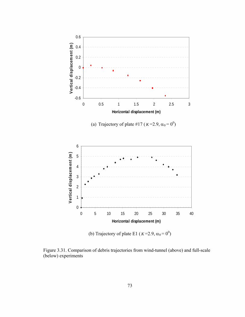
73

-0.6

-0.4

-0.2

0

0.2

0.4

0.6

0 0.5 1 1.5 2 2.5 3


Verti

cal d

ispl

acem

ent (

m)

(a) Trajectory of plate #17 ( K =2.9, α0 = 00)

0

1

2

3

4

5

6

0 5 10 15 20 25 30 35 40


Vert

ical

dis

plac

emen

t (m

)

(b) Trajectory of plate E1 ( K =2.9, α0 = 00)

Figure 3.31. Comparison of debris trajectories from wind-tunnel (above) and full-scale (below) experiments

74

0

0.2

0.4

0.6

0.8

1

0 0.2 0.4 0.6 0.8

Time (sec)

plat

e sp

eed

/ win

d sp

eed

Um

Um (ds/dt)

um

um (dx/dt)

(a) Non-dimensional velocities of #17 ( K =2.9, α0 = 00)

0

0.2

0.4

0.6

0.8

1

0 0.5 1 1.5 2

Time (sec)

plat

e sp

eed

/ win

d sp

eed

Um

Um (ds/dt)

um

um (dx/dt)

(b) Non-dimensional velocities of E1 ( K =2.9, α0 = 00)

Figure 3.32. Comparison of debris velocities from wind-tunnel (above) and full-scale (below) experiments


dtdsum /=


dtdsum /=

75

0

0.2

0.4

0.6

0.8

1

1.2

0.00 0.01 0.10 1.00 10.00

full-scale platesplates #1-#22cubes c1-c6spheres s1-s5rods r1-r8

Figure 3.33. Comparison of debris horizontal trajectories from wind-tunnel and full-scale tests (C denotes the empirical coefficients 911.0=pC , 809.0=cC , 496.0=sC , and

801.0=rC , for plates, cubes, spheres, and rods, respectively.)

3.5 Application to Debris Impact Criteria

The wind-tunnel tests were conducted in uniform flows, while the wind flow in

the atmospheric boundary layers is turbulent. However, full-scale debris flight usually

last only a couple of seconds and is determined by the 2-3 gust speed (Holmes et. al.,

2004). Thus the empirical Equation (3.6) can be used to approximate the debris

horizontal impact speed at a given distance using an average gust speed. The data can be

used to establish debris horizontal impact criteria.

As application examples, Figure 3.34 shows the horizontal speed of a roof tile,

Figure 3.35 of a 2 g, 8 mm steel ball, Figure 3.36 of a 4.1 kg (9 lb) ‘2 by 4’ missile, and

Figure 3.37 a 6.8 kg (15 lb) ‘2 by 4’ missile, respectively. Empirical estimations agree

well with the numerical solutions by Holmes et al. (2004) and Holmes et al. (2005).

u

xCK

76

Although roof tiles have been observed to be the major windborne debris in south

Florida, following Hurricane Andrew in 1992, SFBC (1997) still recommended ‘2 by 4’

timbers as representative debris due to the difficulties in defining a representative roofing

tile. Roof tiles also produced great damage during Hurricane ‘Charley’ in 2004 (Holmes

et al., 2005). The empirical Equation (3.6) provides a convenient approximation for the

speed of plate-like debris. ASTM standards (E1886-97, 1997) specified a steel ball as the

‘small missile’ representative with impact speed between 0.40 and 0.75 of the basic wind

speed (3-s gust in accordance with ANSI/ASCE 7), and ‘2 by 4’ missiles as

representatives of the ‘large missile’ with impact speed between 0.1 and 0.55 of the basic

wind speed. These specified impact speed ranges are covered by the empirical and

numerical solutions, which are speed curves increasing with flight distance. These

specifications may overestimate or underestimate actual debris impact speeds, depending

on how far the debris travels before impact.

It should be noted that impact speed increases with flight distance; however,

debris may have fallen to the ground before reaching the object of interest. Therefore, it

is rational to first estimate potential travel distance of debris with one of Equations (3.8)-

(3.12). Debris flight time is in the order of one or two seconds. Exact debris potential

flight time before hitting the ground depends on the initial height of debris and the

vertical trajectory.

It was also observed that, for plates and rods, the contribution of vertical speed to

resultant speed was very small, because the lift force sustained the debris flight (Figs.

3.38 and 3.39); however, 3D debris fell in the tests and had relatively large contribution

of vertical speed. Actual debris vertical speeds depend on debris vertical displacement.

Investigation of debris vertical trajectory is recommended as a topic for the further

research.

77

0

0.2

0.4

0.6

0.8

1

0.00 10.00 20.00 30.00 40.00 50.00 60.00


Hor

izon

tal v

eloc

ity /

win

d sp

eed

Empirical Eq.(3.6)

Numerical (Holmes et al., 2005)

Figure 3.34. Trajectory of a concrete tile (300 x 300 x 15mm, 3.1kg, 0α =00)

0

0.2

0.4

0.6

0.8

1

0.00 20.00 40.00 60.00 80.00 100.00 120.00


Hor

izon

tal v

eloc

ity /

win

d sp

eed

Empirical Eq.(3.6)Numerical (Holmes et al., 2004)

Figure 3.35. Trajectory of a steel ball (8mm, 2g)

σ+u

σ−u

σ+u

σ−u

78

0

0.2

0.4

0.6

0.8

1

0.00 20.00 40.00 60.00 80.00 100.00


Hor

izon

tal v

eloc

ity /

win

d sp

eed

Empirical Eq.(3.6)

Numerical (Holmes)

Figure 3.36. Trajectory of a ‘2 by 4’ missile (2.4 x 0.1x 0.05m, 4.1kg, 0α =00)

0

0.2

0.4

0.6

0.8

1

0.00 20.00 40.00 60.00 80.00 100.00


Hor

izon

tal v

eloc

ity /

win

d sp

eed

Empirical Eq.(3.6)

Numerical (Holmes)

Figure 3.37. Trajectory of a ‘2 by 4’ missile (4.0 x 0.1 x 0.05m, 6.8kg, 0α =00)

σ+u

σ−u

σ+u

σ−u

79

0

0.2

0.4

0.6

0.8

1

1.2

0.00 1.00 2.00 3.00 4.00 5.00

Horizontal speed

Resultant speed

Figure 3.38. Comparison of horizontal speed and resultant speed of plates ( pC = 0.911)

0

0.2

0.4

0.6

0.8

1

0.00 1.00 2.00 3.00

Horizontal speed

Resultant speed

Figure 3.39. Comparison of horizontal speed and resultant speed of rods ( rC = 0.801)

Debris speed / wind speed

xK

xK

xKC peu 21 −−=

xKCreu 21 −−=

Debris speed / wind speed

80

CHAPTER IV

SUMMARY AND RECOMANDATIONS

4.1 Summary

The primary goal of this research was to investigate the aerodynamic

characteristics of flying debris using wind-tunnel simulation. This knowledge will

facilitate the establishment of rational debris impact criteria and debris risk analysis.

Chapter 1 introduced the published studies on debris identification, debris

initiation, debris trajectory, and debris risk analysis. This research used Wills et al.’s

(2002) classification to study flight trajectories of cubes and spheres (3D), plates (2D),

and rods (1D). Debris initiation may influence debris trajectory and the release wind

speed can be assumed to be constant during debris trajectory. Tachikawa (1983) first

combined experimental and numerical studies on debris trajectory and established non-

dimensional equations of debris motion. The present research followed his pioneering

work. Numerical studies of debris trajectory by Holmes et al. (2004 and 2005) and Baker

(2004) also provided significant information and guided this research. Twisdale et al.

(1996) developed an analysis framework for debris impact risk. A proper debris

trajectory model is critical in debris risk analysis and the present study develops this

knowledge.

Chapter 2 described the wind-tunnel and full-scale tests. Extensive wind-tunnel

simulations of trajectories of 3D, 2D, and 1D debris were carried out. The test design, test

setup and procedure, and data analysis methods were introduced. The procedure can also

be used to study trajectories of irregular debris. Full-scale simulation of debris

trajectories was explored. Full-scale tests can provide calibration data for model-scale

tests.

Chapter 3 presented all the experimental data. Debris trajectories vary with the

characteristics of wind field, debris properties, and debris initial support. The Tachikawa

parameter, K , debris side ratio, and debris initial support configuration were found to

influence the debris trajectory. However, the Tachikawa parameter K governs the

81

horizontal trajectory of debris. Therefore, different debris types at different initial support

situations presented comparable non-dimensional horizontal trajectories. Furthermore,

based on theoretical equations of debris motion, K was combined into non-dimensional

flight variables, resulting in aerodynamic functions for horizontal debris trajectory (Eqs.

3.6-3.12). Good agreement was obtained when compared with numerical solutions.

Application examples of these functions were shown. ASTM standards ignored that

debris flight speed is a function of travel distance. These functions can be applied to

establish rational debris impact criteria

4.2 Recommendations for Further Research

Windborne debris problem is probabilistic in nature. Further research is

recommended to incorporate experimental debris trajectory models into debris risk

analysis. This study has established aerodynamic functions for debris horizontal

trajectory. Combining this knowledge with Monte Carlo simulations, the probability of

debris attaining a damage threshold (velocity, energy, or momentum) at impact can be

qualified. Further investigation of debris vertical trajectory is necessary to predict debris

flight time, which will decide debris travel distance and the probability of impact on a

target.

The use of data from field surveys of actual debris damage to calibrate

experimental models is also recommended for further studies.

82

BIBLIOGRAPHY

American Society for Testing Materials (1997). Standard test method for performance of exterior windows, curtain walls, doors, and storm shutters impacted by missile(s) and exposed to cyclic pressure differentials, ASTM E 1886-97.

Baker, C.J. (2004). Solutions of the debris equations, In : Proc. 6th U.K. Conference on

Wind Engineering, Cranfield, September 15-17, 2004. Holmes, J.D. (2003). Emerging issues in wind engineering. In : Proc. 11th International

Conference on Wind Engineering(11ICWE), Lubbock, Texas, June 2-5, 2003. Holmes, J.D. (2004). Trajectories of spheres in strong winds with application to

windborne debris. Journal of Wind Engineering and Industrial Aerodynamics, 92, 9-22.

Holmes, J.D., and English, E.C. (2004). Aerodynamics and trajectories of windborne

debris, part 1: compact objects, part 2: sheet objects. In : Proc. 11th Australasian Wind Engineering Society Workshop, Darwin, Australia, June 28-29, 2004.

Holmes, J.D., Letchford, C.W., and Lin, N. (2005). Investigations of plate-type windborne debris, II. Computed trajectories, submitted to Journal of Wind Engineering and Industrial Aerodynamics.

Lee, A.J.H. (1974). A general study of tornado-generated missiles. Nuclear Engineering

and Design, 30, 418-433. Lee, B.E. and Wills J. (2002). Vulnerability of fully glazed high-rise buildings in tropical

cyclones. Journal of Architectural Engineering, Vol. 8, No. 2. Letchford, C. W. (2000). Analysis of the propeller wash from a C-130 Hercules aircraft,

WISE Report for NIST, August 2000, Texas Tech University.

Lin, N., Letchford, C.W., and Holmes, J.D. (2005). Investigations of plate-type windborne debris, I. Experiments in wind tunnel and full scale, submitted to Journal of Wind Engineering and Industrial Aerodynamics.

McDonald, J.R., Mehta, K.C., and Minor, J.E. (1974). Tornado-resistant design of

nuclear power-plant structures. Nuclear Safety, Vol. 15, No.4. 432-439. McDonald, J.R. (1976). Tornado-generated missiles and their effects. In : Proc.

Symposium on Tornadoes, Texas Tech University, Lubbock, Texas, June 22-24, 1976.

83

McDonald, J.R. and Kiesling, E.W. (1988). Impact resistance of wood and wood

products to simulated tornado missiles. In : Proc. International Conference on Timber Engineering, Seattle, WA, September 19-22, 1988.

McDonald, J.R. (1990). Impact resistance of common building materials to tornado

missiles. Journal of Wind Engineering and Industrial Aerodynamics, 36, 717-742. McDonald, J.R. (1999). Windborne debris impacts on metal wall panels and their

implications. Wind Engineering into the 21st Century, Larsen, Larose & Livesey (eds), Balkema, Rotterdam, ISBN 90 5809 059 0, 1443-1449.

Minor, J.E. (1994). Windborne debris and the building envelope. Journal of Wind

Engineering and Industrial Aerodynamics, 53, 207-227. Redmann, G.H, Radbill, J.R., Marte, J.E., Degarabedian, P., and Fendell, F.E.(1976).

Wind field and trajectory models for tornado propelled objects. Electrical Power Research Institute, Technical Report 1, Palo Alto, CA.

SFBC (1997). South Florida building code, Dade County edition. Simiu, E. and Cordes, M. (1976). Tornado borne missile speeds. NBSIR 76-1050,

National Bureau of Standards. Tachikawa, M (1983). Trajectories of flat plates in uniform flow with application to

wind-generated missiles. Journal of Wind Engineering and Industrial Aerodynamics, 14, 443-453.

Tachikawa, M (1988). A method for estimating the distribution range of trajectories of

wind-borne missiles. Journal of Wind Engineering and Industrial Aerodynamics, 29, 175-184.

Twisdale, L.A., Dunn, W.L., and Davis, T.L. (1979). Tornado missile transport analysis.

Nuclear Engineering and Design, 51, 295-308. Twisdale, L.A., Vickery, P.J., and Steckley, A.C. (1996). Analysis of hurricane

windborne debris impact risk for residential structures, prepared for State Farm Mutual Automobile Insurance Companies.

Wang, K. and Letchford, C.W. (2003). Flying debris behavior. In : Proc. Eleventh

International Conference on Wind Engineering(11ICWE), Lubbock, Texas, June 2-5, 2003.

84

Wills, J.A.B., Lee, B.E., and Wyatt, T.A. (2002). A model of wind-borne debris damage. Journal of Wind Engineering and Industrial Aerodynamics, 90, 555-565.

PERMISSION TO COPY

In presenting this thesis in partial fulfillment of the requirements for a master’s

degree at Texas Tech University or Texas Tech University Health Sciences Center, I

agree that the Library and my major department shall make it freely available for research

purposes. Permission to copy this thesis for scholarly purposes may be granted by the

Director of the Library or my major professor. It is understood that any copying or

publication of this thesis for financial gain shall not be allowed without my further

written permission and that any user may be liable for copyright infringement.

Agree (Permission is granted.)

Ning Lin ______________ ___ ___ June 29, 2005___ Student Signature Date Disagree (Permission is not granted.) _______________________________________________ _________________ Student Signature Date

SIMULATION OF WINDBORNE DEBRIS TRAJECTORIES by NING

Documents

Transcript of SIMULATION OF WINDBORNE DEBRIS TRAJECTORIES by NING