1

Simulation of sun sensors using STK

Han Gao, Jinxu Huang, Steen Eiler Jørgensen, Daniel Umicevic, Linlin Wang, Krzysztof Wojtanowicz and Ying Yan

1 Project definition The project definition reads:

“Based on models of sun sensors, the Satellite’s attitude in space is simulated in STK and vectors show the expected output signal from the sun sensors. The simulation is compared with real data collected in field tests on the DTUsat flight. The simulation will be used in the public outreach activities for DTUsat 1.”

As it will be seen, we did succeed in simulating the satellite’s attitude in STK, and converting the output azimuth and elevation angles to the Sun to sun sensor output values. We believe using vectors to display the values returned from the sun sensors is an impractical way of visualizing the output from the sensors. Instead, we would find it more relevant to display the values in the Data Display window of STK. However, this involves transmitting data “live” forwards and backwards between STK and MATLAB. This is described in the documentation for STK1, and involves creating files and folders on drive C: which is not possible on the DTU databar computers, due to user access restrictions. Using “plug-in scripts”, it should in principle be possible to get STK to display values computed in MATLAB. Also, we have not compared simulated data with real data from the field tests, since we only received the bare data files, and no documentation as to how to interpret these data, coordinate system definitions, etc. 3 Sensor definitions A sun sensor is shown in figure 1. Each sensor is able to measure the angle to the sun along its own axis. For a thorough description of the sun sensors, refer to Hales and Pedersen: Two-Axis MOEMS Sun Sensor for Pico Satellites [1]. If we know the direction to the Sun relative to the satellite body’s reference system, we are in principle able to calculate, what output the twelve sun sensors will yield. The satellite is cubic in shape. There are two sun sensors on each of the satellite’s six sides. The sensors are perpendicular to each other. The sensors return an angular value based on the direction to the sun in the plane defined by the sensor as seen from the sensor. A Cartesian coordinate system is defined with axes x, y and z, that are normal to three sides of the satellite. Instead of referring to the planes spanned by these axes as xy, xz and yz, we define X as the yz-plane, normal to the x-axis, Y as the xz-plane, normal to the y-axis, and Z as the xy-plane, normal to the z-axis. This means, that

1 C:/Program Files/AGI/stk/4.3/manuals/pluginScripts.pdf

2

Figure 1: A sun sensor mounted on a PCB. one sensor is located in the X-plane parallel to the y-axis, denoted XY, one sensor is located in the X-plane parallel to the z-axis, denoted XZ, one sensor is located in the Y-plane parallel to the x-axis, denoted YX, one sensor is located in the Y-plane parallel to the z-axis, denoted YZ, one sensor is located in the Z-plane parallel to the x-axis, denoted ZX, and one sensor is located in the Z-plane parallel to the y-axis, denoted ZY. Of course, there are also sensors on the six “negative” sides of the satellites, denoted with a leading minus. The sensors are defined to give a positive value in the direction of the axes, to which they are parallel. Thus, a sensor seeing the sun directly overhead will return a value of 0°. If the angle to the sun α < –90° or α > 90°, then the sensor cannot see the sun. In the satellite’s xyz reference system, the direction to the sun is defined by two angles:

θ – the azimuthal angle in the xy-plane measured from the x-axis towards the y-axis, and φ – the elevation angle, measuring the angular distance from the xy-plane. It is seen, that –180° < θ ≤ 180° and –90° ≤ φ ≤ 90°. We have established relationships between θ and φ and the measured angles from the sun sensors. The geometric considerations and derived formulas are given in appendix 1. Bear in mind, that – before applying constraints – the sensor values should be in the range [–90°;90°] 4 Using STK The satellite was defined in STK by constructing its orbit. The DTUsat orbit was defined as a circular, sun-synchronous orbit with a height over the Earth’s surface of 820 km. This yielded following values for the first three classical orbital elements:

3

semimajor axis a = 7198.137000 km eccentricity e = 0.00000000 inclination i = 98.692783° We also constructed a cubical model of the satellite. The model file, dtusat.mdl, was edited in Windows Notepad. Due to the lack of documentation on the structure of .mdl-files, we had to construct the satellite model by trial-and-error. It proved not too difficult, however. The name “sun sensors” imply that it appears self-evident, that we should use the “Sensor” tool in STK. However, all our attempts to make the sensors “sense” the sun were futile. As it turned out, the most powerful tools in STK in this context were the “Report Style Properties” window in combination with the “Vector Geometry Tool”.

Figure 2: DTUsat 1 simulation in STK. The red, green and blue axes indicate the xyz coordinate system of the satellite body. The yellow vector indicates the direction to the Sun.

The difficult part was to obtain the direction to the sun in the non-inertial satellite body reference system. After having spent several days trying to figure out how to define a plane, and how to read out the angle between a vector and this plane, we finally found out, that we should define a new “Report style” using the following procedure:

4

Figure 3: Selecting the “Report” tool in STK.

Figure 4: Selecting values to be written out to the report.

5

1. Right-click on DTUsat 1 in STK 2. Choose “Report” (See figure 3) 3. Under “Style”, choose “New” 4. Under “Style”, choose “Properties” 5. Under “Elements”, open “Lighting AER” and choose “BodyFixed” (See figure 4) 6. Choose desired elements. We chose Azimuth and Elevation2. Click OK 7. In the Report Tool, choose “Create…”, and the report is created. 8. Under “File”, choose “Export…” and save the file as filename.dat

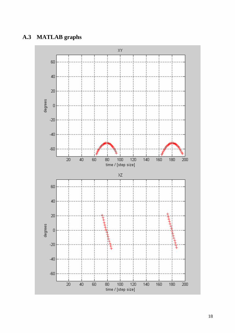
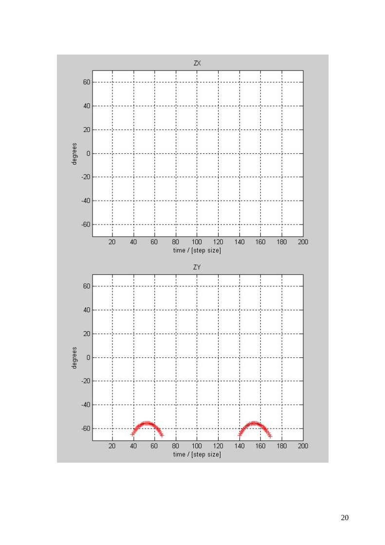
This way, we are able to output the azimuth and elevation angles to the sun relative to the coordinate system fixed in the satellite body. These values are used in MATLAB to calculate the output from the sun sensors. We simulated values of θ and φ for DTUsat 1 in a – hopefully! – not entirely unrealistic attitude situation: “Nadir alignment with ECF velocity constraint”. In this case, the satellite has its z-axis pointing towards the center of the Earth, and the x-axis pointing in the satellite’s direction of motion. In this simulation, the Sun primarily shines on the –Y face, which can also be seen on the graphs for sensors –YX and –YZ in appendix 2. 5 Using MATLAB In MATLAB, a program was created, which takes the azimuth and elevation values in the report generated by STK and converts them into sun sensor output readings. Before reading the report file into MATLAB, we had to remove the first line of text in the file. We did this by opening the data file in WordPad, deleting the first line of text and saving the file. The tricky part was to figure out the mathematical formulas. Since the readings from the sun sensors are directly connected to the azimuth and elevation angles, it should be (and probably is) possible to determine formulas, that always yield the right values for the sensors on the positive sides of the satellite. Knowing these, it should be trivial to compute the readings on the negative sides. However, we were not able to derive these precise formulas. Instead, we were able to derive formulas, that are valid only in specific ranges of values of θ and φ, and then use conditional programming to calculate the values. The MATLAB program, sun_sensor_output.m, is shown in appendix 1. The output graphs showing the sun sensors values as a function of time is shown in appendix 2. 6 Conclusion We succeeded in simulating the output from the sun sensors as a function of the values for azimuth and elevation angles to the sun as seen from the satellite body’s reference system. Due to technical problems, we have not experimented with the close cooperation between STK and MATLAB made possible by the plug-in scripts function in STK. Due to lack of time – and understanding of the format of the data files – we haven’t compared the simulated values to real data. Also, in our simulation, we have not taken into account the refraction of the sunlight due to the thin layer of silicon on top of the sun sensors.

2 If time is included in the report, MATLAB is not able to read this data – at least, we did not succeed in persuading MATLAB to read this data.

6

We haven’t actually converted the sun sensor angles into solar cell currents, since we didn’t deem it necessary – the conversion to angles should take place in the onboard computer. The output from the sun sensors is based only on the direction to the sun as seen from the satellite. Thus, the shadowing effect from the earth has not been taken into account. This would involve dumping orbital data to MATLAB as well as the azimuth and elevation angles, and we have not considered this. The reason for this is, that this is only a simulation of the output from the sun sensors. In reality, it will not be that difficult to determine, if the satellite is in shadow – if none of the sun sensors are returning data, the satellite is probably in shadow! The probably most useful work still remains to be done: a routine for converting the output from the sun sensors into an actual attitude value. This is a fine project for future teams in this course ☺.

7

A.1 Geometric analysis and derivation of formulas Mathematical relations between θ and φ and the values output from the sun sensors

Face angle θ φ XY = θ (–90°;90°) (–90°;90°) YX = 90° – θ (0;180°) (–90°;90°)

YZ = Arctan

θφ

sintan

(0;180°) (–90°;90°)

ZY = 90° – arctan

θφ

sintan

<0;180°> (0;90°>

ZY = –90° – arctan

θφ

sintan

(–180°;0) (0;90°>

XZ = arctan

θφ

costan

(–90°;90°) (–90°;90°)

ZX = 90° – arctan

θφ

costan

<–90;90°> (0;90°>

ZX = –90° – arctan

θφ

costan

<–180°;–90°)∪(90°;180°> (0;90°>

Face angle θ φ

–XY = 180° – θ (90°;180°> (–90°;90°) –XY = –180° – θ (–180°;–90°) (–90°;90°) –YX = 90° +θ (–180°;0) (–90°;90°)

–YZ = –arctan

θφ

sintan

(–180°;0) (–90°;90°)

–XZ = –arctan

θφ

costan

(–180°;–90°)∪(90°;180°> (–90°;90°)

–ZX = 90° + arctan

θφ

costan

<–90°;90°> <–90°;0)

–ZX = –90° + arctan

θφ

costan

<–180°;–90°)∪(90°;180°> <–90°;0)

–ZY = 90° + arctan

θφ

sintan

<0;180°> <–90°;0)

–ZY = –90° + arctan

θφ

sintan

(–180°;0) <–90°;0)

Initial Constraints:

θ ∈ <–180°;180°> φ ∈ <–90°;90°>

8

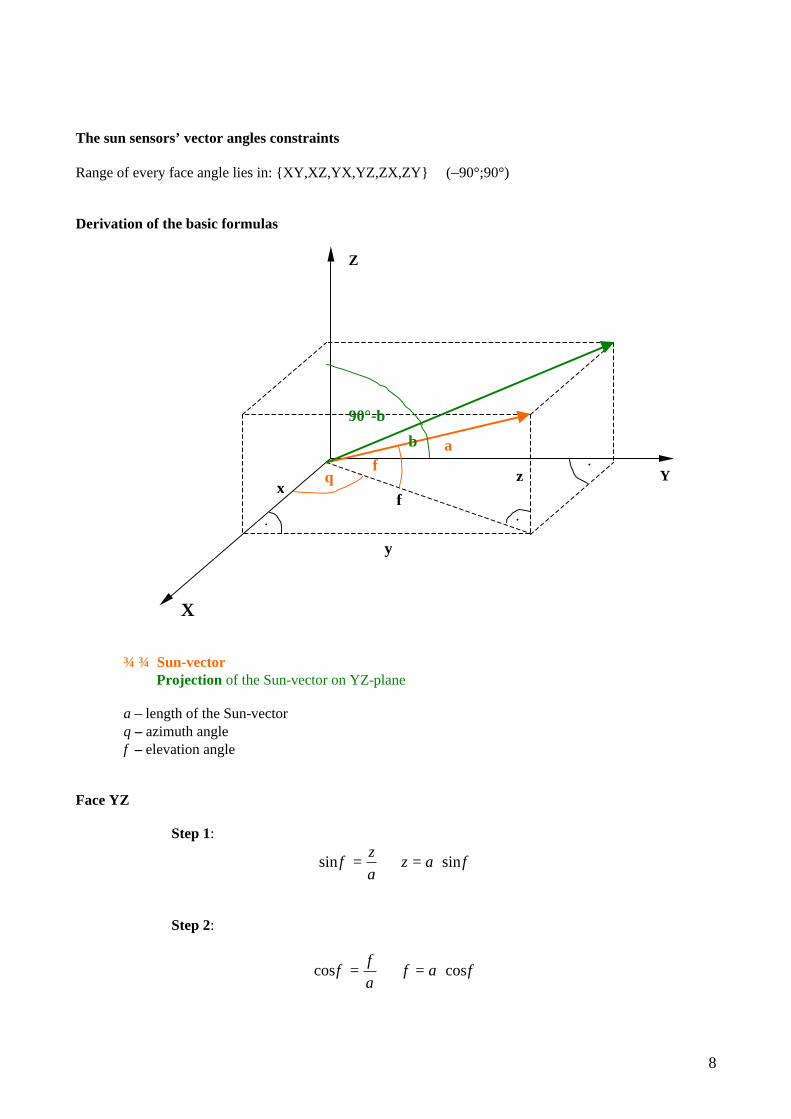
The sun sensors’ vector angles constraints Range of every face angle lies in: {XY,XZ,YX,YZ,ZX,ZY} ∈ (–90°;90°) Derivation of the basic formulas

Sun-vector Projection of the Sun-vector on YZ-plane

a – length of the Sun-vector θ – azimuth angle φ – elevation angle

Face YZ

Step 1:

φφ sinsin ⋅=⇒= azaz

Step 2:

φφ coscos ⋅=⇒= afaf

f

Z

X

Y

y

x z

• •

• φ θ

β a

90°-β

9

φθφ

θ cossincos

sin ⋅⋅=⇒⋅

== aya

yfy

Step 3:

φθφ

βcossin

sintan

⋅⋅⋅

==a

ayz

θφ

βsintan

tan =

=

θφ

βsintan

arctan

=

θφ

sintan

arctanYZ

Face ZY: This face is based on the angle YZ

ZY = 90° − β

−°=

θφ

sintan

arctan90ZY

f

Z

X

Y

y

x z

• •

• φ θ

β a

90°-β

10

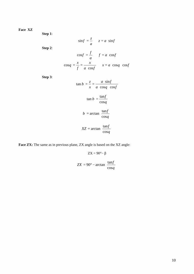
Face XZ Step 1:

φφ sinsin ⋅=⇒= azaz

Step 2:

φφ coscos ⋅=⇒= afaf

φθφ

θ coscoscos

cos ⋅⋅=⇒⋅

== axa

xfx

Step 3:

φθφ

βcoscos

sintan

⋅⋅⋅

==a

axz

θφ

βcostan

tan =

=

θφ

βcostan

arctan

=

θφ

costan

arctanXZ

Face ZX: The same as in previous plane, ZX angle is based on the XZ angle:

ZX = 90°− β

−°=

θφ

costan

arctan90ZX

11

Face XY: In this case, after projection of the Sun-vector on the XY-plane, the angle of XY will be the same as β-Azimuth angle. Face YX: Value of angle YX is equal to the difference of 90° and XY angle. Note: If the angle of θ or φ is not continuous over the given range, than the formula for given face must be split (depends on number of discontinuities).

f

Z

X

Y

y

x z

• •

• φ θ=β

a

90°-β

12

A.2 MATLAB program dtusat = importdata('output4.dat'); data = dtusat; % Number of time steps to display steps = 200 % Get data from file theta = data(:,1); phi = data(:,2); % Conversion of angles from degrees to radians theta_rad = theta*pi/180; phi_rad = phi*pi/180; for n = 1:length(theta) % Determination of which angles to calculate if theta(n) <= 90 & theta(n) >= -90 x = 1; else x = -1; end if theta(n) >= 0 & theta(n) < 180 y = 1; else y = -1; end if phi(n) >= 0 z = 1; else z = -1; end % Calculation of sun sensor angles if x == 1 xy(n) = theta_rad(n); xz(n) = atan(tan(phi_rad(n))/cos(theta_rad(n))); mxy(n) = -pi/2; mxz(n) = -pi/2; else xy(n) = -pi/2; xz(n) = -pi/2; mxy(n) = pi-theta_rad(n); if mxy(n) > pi mxy(n) = -(2*pi-mxy(n)) end mxz(n) = -atan(tan(phi_rad(n))/cos(theta_rad(n))); end

13

if y == 1 yx(n) = pi/2-theta_rad(n); yz(n) = atan(tan(phi_rad(n))/sin(theta_rad(n))); myx(n) = -pi/2; myz(n) = -pi/2; else yx(n) = -pi/2; yz(n) = -pi/2; myx(n) = pi/2-theta_rad(n); if myx(n) > pi/2 myx(n) = pi-myx(n); end myz(n) = -atan(tan(phi_rad(n))/sin(theta_rad(n))); end if z == 1 zx(n) = pi/2-atan(tan(phi_rad(n))/cos(theta_rad(n))); if zx(n) > pi/2 zx(n) = zx(n)-pi end zy(n) = pi/2-atan(tan(phi_rad(n))/sin(theta_rad(n))); if zy(n) > pi/2 zy(n) = zy(n)-pi end mzx(n) = -pi/2; mzy(n) = -pi/2; else zx(n) = -pi/2; zy(n) = -pi/2; mzx(n) = pi/2-atan(tan(-phi_rad(n))/cos(theta_rad(n))); if mzx(n) > pi/2 mzx(n) = mzx(n)-pi end mzy(n) = pi/2-atan(tan(-phi_rad(n))/sin(theta_rad(n))); if mzy(n) > pi/2 mzy(n) = mzy(n)-pi end end end % Conversion of angles from radians to degrees xy = xy*180/pi; xz = xz*180/pi; yx = yx*180/pi; yz = yz*180/pi; zx = zx*180/pi; zy = zy*180/pi; mxy = mxy*180/pi; mxz = mxz*180/pi; myx = myx*180/pi; myz = myz*180/pi; mzx = mzx*180/pi; mzy = mzy*180/pi;

14

% Constraints on sensors due to exceeded field of view in sensor direction for n = 1:length(xy) % Plane x if xy(n) < -70 | xy(n) > 70 xy(n) = -90; end if xz(n) < -70 | xz(n) > 70 xz(n) = -90; end % Plane y if yx(n) < -70 | yx(n) > 70 yx(n) = -90; end if yz(n) < -70 | yz(n) > 70 yz(n) = -90; end % Plane z if zx(n) < -70 | zx(n) > 70 zx(n) = -90; end if zy(n) < -70 | zy(n) > 70 zy(n) = -90; end % Plane -x if mxy(n) < -70 | mxy(n) > 70 mxy(n) = -90; end if mxz(n) < -70 | mxz(n) > 70 mxz(n) = -90; end % Plane -y if myx(n) < -70 | myx(n) > 70 myx(n) = -90; end if myz(n) < -70 | myz(n) > 70 myz(n) = -90; end % Plane -z if mzx(n) < -70 | mzx(n) > 70 mzx(n) = -90; end if mzy(n) < -70 | mzy(n) > 70 mzy(n) = -90; end end

15

% Constraints on sensors due to exceeded field of view perpendicular to sensor direction for n = 1:length(xy) % Plane x tmp = xy(n) if xz(n) < -55 | xz(n) > 55 xy(n) = -90; end if tmp < -55 | tmp > 55 xz(n) = -90; end % Plane y tmp = yx(n) if yz(n) < -55 | yz(n) > 55 yx(n) = -90; end if tmp < -55 | tmp > 55 yz(n) = -90; end % Plane z tmp = zx(n) if zy(n) < -55 | zy(n) > 55 zx(n) = -90; end if tmp < -55 | tmp > 55 zy(n) = -90; end % Plane -x tmp = mxy(n) if mxz(n) < -55 | mxz(n) > 55 mxy(n) = -90; end if tmp < -55 | tmp > 55 mxz(n) = -90; end % Plane -y tmp = myx(n) if myz(n) < -55 | myz(n) > 55 myx(n) = -90; end if tmp < -55 | tmp > 55 myz(n) = -90; end % Plane -z tmp = mzx(n)

16

if mzy(n) < -55 | mzy(n) > 55 mzx(n) = -90; end if tmp < -55 | tmp > 55 mzy(n) = -90; end end % Plotting results figure(1) plot(xy,'r+'); grid on xlabel('time / [step size]'); ylabel('degrees'); title('XY'); axis([-Inf steps -70 70]) figure(2) plot(xz,'r+'); grid on xlabel('time / [step size]'); ylabel('degrees'); title('XZ'); axis([-Inf steps -70 70]) figure(3) plot(yx,'r+'); grid on xlabel('time / [step size]'); ylabel('degrees'); title('YX'); axis([-Inf steps -70 70]) figure(4) plot(yz,'r+'); grid on xlabel('time / [step size]'); ylabel('degrees'); title('YZ'); axis([-Inf steps -70 70]) figure(5) plot(zx,'r+'); grid on xlabel('time / [step size]'); ylabel('degrees'); title('ZX'); axis([-Inf steps -70 70]) figure(6) plot(zy,'r+'); grid on xlabel('time / [step size]'); ylabel('degrees'); title('ZY'); axis([-Inf steps -70 70]) figure(7)

17

plot(mxy,'r+'); grid on xlabel('time / [step size]'); ylabel('degrees'); title('-XY'); axis([-Inf steps -70 70]) figure(8) plot(mxz,'r+'); grid on xlabel('time / [step size]'); ylabel('degrees'); title('-XZ'); axis([-Inf steps -70 70]) figure(9) plot(myx,'r+'); grid on xlabel('time / [step size]'); ylabel('degrees'); title('-YX'); axis([-Inf steps -70 70]) figure(10) plot(myz,'r+'); grid on xlabel('time / [step size]'); ylabel('degrees'); title('-YZ'); axis([-Inf steps -70 70]) figure(11) plot(mzx,'r+'); grid on xlabel('time / [step size]'); ylabel('degrees'); title('-ZX'); axis([-Inf steps -70 70]) figure(12) plot(mzy,'r+'); grid on xlabel('time / [step size]'); ylabel('degrees'); title('-ZY'); axis([-Inf steps -70 70])

18

A.3 MATLAB graphs

19

20

21

22

23

24

References [1] Jan H. Hales and Martin Pedersen: Two-Axis MOEMS Sun Sensor for Pico Satellites, 16th Annual AIAA/USU Conference on Small Satellites, 2002