SIMULATION OF RESISTIVITY LOGGING-WHILE … · SIMULATION OF RESISTIVITY LOGGING-WHILE-DRILLING...
21
SIMULATION OF RESISTIVITY LOGGING-WHILE-DRILLING (LWD) MEASUREMENTS USING A SELF-ADAPTIVE GOAL-ORIENTED HP FINITE ELEMENT METHOD. D. PARDO † , ‡ , L. DEMKOWICZ † , C. TORRES-VERD ´ IN ‡ , AND M. PASZYNSKI † , § Abstract. We simulate electromagnetic (EM) measurements acquired with a Logging-While- Drilling (LWD) instrument in a borehole environment. The measurements are used to assess electrical properties of rock formations. Logging instruments as well as rock formation properties are assumed to exhibit axial symmetry around the axis of a vertical borehole. The simulations are performed with a self-adaptive goal-oriented hp-Finite Element Method (FEM) that delivers exponential convergence rates in terms of the quantity of interest (for exam- ple, the difference in the electrical current measured at two receiver antennas) against the CPU time. Goal-oriented adaptivity allows for accurate approximations of the quantity of interest with- out the need of obtaining an accurate solution in the entire computational domain. In particular, goal-oriented hp-adaptivity becomes essential to simulate LWD instruments, since it reduces the computational cost by several orders of magnitude with respect to the global energy-norm based hp-adaptivity. Numerical results illustrate the efficiency and high-accuracy of the method, and provide physical interpretation of resistivity measurements obtained with LWD instruments. These results also de- scribe the advantages of using magnetic buffers in combination with solenoidal antennas for strength- ening the measured EM signal so that the ’signal-to-noise’ ratio is minimized. Key words. hp-finite elements, exponential convergence, goal-oriented adaptivity, computa- tional electromagnetics, Maxwell’s equations, through casing resistivity tools (TCRT). AMS subject classifications. 78A25, 78A55, 78M10, 65N50 1. Introduction. A plethora of energy-norm based algorithms intended to gen- erate optimal grids have been developed throughout the last decades (see, for example, [7, 18] and references therein) to accurately solve a large class of engineering prob- lems. However, the energy-norm is a quantity of limited relevance for most engineering applications, especially when a particular objective is pursued, for instance, to sim- ulate the electromagnetic response of geophysical resistivity logging instruments in a borehole environment. In these instruments, the amplitude of the measurement (for example, the electric field) is typically several orders of magnitude smaller at the receiver antennas than at the transmitter antennas. Thus, small relative errors of the solution in the energy-norm do not imply small relative errors of the solution at the receiver antennas. Indeed, it is not uncommon to construct adaptive grids delivering a relative error in the energy-norm below 1% while the solution at the receiver antennas still exhibits a relative error above 1000% (see [13]). Consequently, in order to accurately simulate LWD resistivity measurements in this paper, we develop a self-adaptive strategy to approximate a specific feature of the solution. Refinement strategies of this type are called goal-oriented adaptive algorithms [11, 17], and are based on minimizing the error of a prescribed quantity of interest mathematically expressed in terms of a linear functional (see [3, 9, 12, 11, 17, 19] for details). † Institute for Computational Engineering and Sciences (ICES), The University of Texas at Austin, Austin TX 78712 ‡ Department of Petroleum and Geosystems Engineering, The University of Texas at Austin, Austin TX 78712 § On leave from AGH University of Science and Technology, Department of Computer Methods in Metallurgy, Cracow, Poland 1
Transcript of SIMULATION OF RESISTIVITY LOGGING-WHILE … · SIMULATION OF RESISTIVITY LOGGING-WHILE-DRILLING...
SIMULATION OF RESISTIVITY LOGGING-WHILE-DRILLING(LWD) MEASUREMENTS USING A SELF-ADAPTIVEGOAL-ORIENTED HP FINITE ELEMENT METHOD.
D. PARDO† ,‡ , L. DEMKOWICZ† , C. TORRES-VERDIN‡ , AND M. PASZYNSKI† ,§
Abstract. We simulate electromagnetic (EM) measurements acquired with a Logging-While-Drilling (LWD) instrument in a borehole environment. The measurements are used to assess electricalproperties of rock formations. Logging instruments as well as rock formation properties are assumedto exhibit axial symmetry around the axis of a vertical borehole.
The simulations are performed with a self-adaptive goal-oriented hp-Finite Element Method(FEM) that delivers exponential convergence rates in terms of the quantity of interest (for exam-ple, the difference in the electrical current measured at two receiver antennas) against the CPUtime. Goal-oriented adaptivity allows for accurate approximations of the quantity of interest with-out the need of obtaining an accurate solution in the entire computational domain. In particular,goal-oriented hp-adaptivity becomes essential to simulate LWD instruments, since it reduces thecomputational cost by several orders of magnitude with respect to the global energy-norm basedhp-adaptivity.
Numerical results illustrate the efficiency and high-accuracy of the method, and provide physicalinterpretation of resistivity measurements obtained with LWD instruments. These results also de-scribe the advantages of using magnetic buffers in combination with solenoidal antennas for strength-ening the measured EM signal so that the ’signal-to-noise’ ratio is minimized.
Key words. hp-finite elements, exponential convergence, goal-oriented adaptivity, computa-tional electromagnetics, Maxwell’s equations, through casing resistivity tools (TCRT).
AMS subject classifications. 78A25, 78A55, 78M10, 65N50
1. Introduction. A plethora of energy-norm based algorithms intended to gen-erate optimal grids have been developed throughout the last decades (see, for example,[7, 18] and references therein) to accurately solve a large class of engineering prob-lems. However, the energy-norm is a quantity of limited relevance for most engineeringapplications, especially when a particular objective is pursued, for instance, to sim-ulate the electromagnetic response of geophysical resistivity logging instruments ina borehole environment. In these instruments, the amplitude of the measurement(for example, the electric field) is typically several orders of magnitude smaller at thereceiver antennas than at the transmitter antennas. Thus, small relative errors of thesolution in the energy-norm do not imply small relative errors of the solution at thereceiver antennas. Indeed, it is not uncommon to construct adaptive grids delivering arelative error in the energy-norm below 1% while the solution at the receiver antennasstill exhibits a relative error above 1000% (see [13]).
Consequently, in order to accurately simulate LWD resistivity measurements inthis paper, we develop a self-adaptive strategy to approximate a specific feature ofthe solution. Refinement strategies of this type are called goal-oriented adaptivealgorithms [11, 17], and are based on minimizing the error of a prescribed quantity of
interest mathematically expressed in terms of a linear functional (see [3, 9, 12, 11, 17,19] for details).
†Institute for Computational Engineering and Sciences (ICES), The University of Texas atAustin, Austin TX 78712
‡Department of Petroleum and Geosystems Engineering, The University of Texas at Austin,Austin TX 78712
§On leave from AGH University of Science and Technology, Department of Computer Methodsin Metallurgy, Cracow, Poland
1

2 D. PARDO, L. DEMKOWICZ, C. TORRES-VERDIN, M. PASZYNSKI
In this paper, we formulate, implement, and study (both theoretically and nu-merically) a self-adaptive hp goal-oriented algorithm intended to solve electrodynamicproblems. This algorithm is an extension of the fully automatic (energy-norm based)hp-adaptive strategy described in [7, 18], and a continuation of concepts presented in[14, 20] for elliptic problems.
We apply the self-adaptive hp goal-oriented algorithm to accurately simulate in-duction LWD instruments in a borehole environment with axial symmetry. Theseinstruments are widely used by the geophysical logging industry, and their simula-tion requires resolution of EM singularities generated by the LWD geometry and rockformation materials [22], as well as resolution of high material constrasts that occurbetween the mandrel and the borehole.
The organization of this document is as follows: In Section 2, we describe themain characteristics of induction logging instruments. We also describe our problemof interest, composed of an induction LWD instrument in a borehole environment,and used for the assessment of the rock formation electrical properties. In Section3, we introduce Maxwell’s equations, governing the electromagnetic phenomena andexplaining the physics of resistivity measurements. We also derive the correspondingvariational formulation for axisymmetric problems. A self-adaptive goal-oriented hpalgorithm for electrodynamic problems is described in Section 4. The correspondingdetails of implementation are discussed in the same section. Simulations and numer-ical results concerning the response of LWD instruments in a borehole environmentare shown in Section 5. Section 6 draws the main conclusions, and outline futurelines of research. Finally, in the Appendix, we compare numerical results with asemi-analytical solution obtained using Bessel functions for a simplified LWD modelproblem. The comparison is intended to verify the code as well as to illustrate thehigh accuracy results obtained with the self-adaptive goal-oriented hp-FEM.
2. Alternate Current (AC) Logging Applications. In this article, we con-sider an induction1 LWD instrument operating at 2 Mhz. The instrument makes useof one of the following two types of source antennas/coils:
• solenoidal coils (Fig. 2.1, left panel), and• toroidal coils (Fig. 2.1, right panel).
2.1. Induction LWD Instruments Based on Solenoidal Coils. For ax-isymmetric problems, these logging instruments generate a TMφ field, i.e., the onlynon-zero components of the electromagnetic (EM) fields are Eφ, Hρ, and Hz, where(ρ, φ, z) denote the cylindrical system of coordinates.
A solenoidal coil (Fig. 2.1) produces an impressed current Jimp that we mathe-matically describe as
Jimp(r) = φIδ(ρ − a)δ(z) ,(2.1)
where I is the electric current measured in Amperes (A), δ is the Dirac’s delta function,and a is the radius of the solenoid. In the numerical computations, we replace functionδ(ρ− a)δ(z) with an approximate function UF that considers the finite dimensions ofthe coil, and such that
∫UF dρdz = 1.
The analytical electric far-field solution excited by a solenoidal coil of radius aradiating in homogeneous media is given in terms of the electric field by (see [10])
1Induction logging instruments are characterized by the fact that impressed current Jimp isdivergence free (i.e., ∇ · Jimp = 0).

HP -FEM: ELECTROMAGNETIC APPLICATIONS 3
Fig. 2.1. Two coil antennas: a solenoid antenna (left panel) composed of a wire wrapped arounda cylinder, and a toroid antenna (right panel) composed of a wire wrapped around a toroid.
E = φωµkIπa2 e−jkd
4πd[1 − j
kd]ρ
d,(2.2)
where k =√
ω2ε − jωσ is the wave number, j =√−1 is the imaginary unit, ω is
angular frequency, ε, µ, and σ stand for dielectric permittivity, magnetic permeabil-ity, and electrical conductivity of the medium, respectively, and d is the distancebetween the source coil and the receiver coil. In order to avoid the dependence uponthe dimensions of the solenoid, we impose a current on the solenoidal coil equal to1/(πa2) A, i.e., equivalent to that of 1 A with a Vertical Magnetic Dipole (VMD).The corresponding far-field solution in homogeneous media is given by (see [10])
E = φωµkIe−jkd
4πd[1 − j
kd]ρ
d.(2.3)
Thus, solution (2.3) is independent of the dimensions of the coil2.
2.2. Induction LWD Instruments Based on Toroidal Coils. For axisym-metric problems, these logging instruments generate a TEφ field, i.e., the only non-zero components of the EM fields are Hφ, Eρ, and Ez.
A toroidal coil induces a magnetic current IM in the azimuthal direction. If weplace a toroid of radius a radiating in homogeneous media, the resulting magneticfar-field is given by (see [10])
H = φ(σ + jωε)πa2IM jke−jkd
4πd[1 − j
kd]ρ
d.(2.4)
In order to avoid the dependence upon the dimensions of the toroid, we impose amagnetic current on the toroidal coil equal to that induced by a (σ + jωε) A electriccurrent excitation with a Vertical Electrical Dipole (VED), also known as Hertzian
2In resistivity logging applications, it is customary to consider solutions that have been divided bythe geometrical factor (also called K-factor) [1], so that results are independent (as much as possible)of the logging instrument’s geometry. Thus, solutions obtained from different logging instrumentscan be readily compared.

4 D. PARDO, L. DEMKOWICZ, C. TORRES-VERDIN, M. PASZYNSKI
dipole. The corresponding magnetic far-field solution in homogeneous media is givenby (see [10])
H = φ(σ + jωε)Ijke−jkd
4πd[1 − j
kd]ρ
d.(2.5)
In this case, IM = I/(πa2).
2.2.1. Goal of the Computations. We are interested in simulating the EMresponse of an induction LWD instrument in a borehole environment.
For a solenoidal coil, the main objective of our simulation is to compute thefirst difference of the voltage between the two receiving coils of radius a divided bythe (vertical) distance ∆z between them, i.e.,
V1 − V2
∆z=
(∮
l1
E(l) dl −∮
l2
E(l) dl
)/(∆z) =
2πa
∆z(E(l1) − E(l2)) ,(2.6)
where l1 and l2 are the first and second receiving coils, respectively, and l1 ∈ l1,l2 ∈ l2 are two arbitrary points located at the receiving coils. Notice that due to theaxisymmetry of the electric field, E(lji ) = E(lki ) for all lji , l
ki ∈ li.
This quantity of interest (first difference of voltage) is widely used in resistivitylogging applications. Indeed, a first-order asymptotic approximation of the electricfield response at low frequencies (Born’s approximation) shows that the voltage at areceiver coil is proportional to the rock formation resistivity in the proximity of sucha coil (see [10] for details). At higher frequencies (> 20 Khz), asymptotic approx-imations (see [1] for details) also indicate the dependence of the voltage upon therock formation conductivity. Thus, an adequate approximation of the rock formationconductivity (which is unknown a priori in practical applications) can be estimatedfrom the voltage measured at the receiving coils. Computing the first difference ofthe voltage between two receivers (rather than the voltage at one receiver) is conve-nient for improving the vertical resolution of the measurements. This well-known factamong well-logging practitioners will be illustrated here with numerical experiments.
For a toroidal coil, the main objective of these simulations is to compute thefirst difference of the electric current at the two receiving coils of radius a divided bythe (vertical) distance ∆z between them, i.e.,
I1 − I2
∆z=
(∮
l1
H(l) dl −∮
l2
H(l) dl
)/(∆z) =
2πa
∆z(H(l1) − H(l2)) .(2.7)
Notice that the main difference between a toroidal and a solenoidal coil is thatthe former generates an impressed magnetic current, while the latter produces animpressed electric current. This fact leads to the physical consideration that, if thevoltage due to a solenoidal coil is proportional to the rock formation conductivity, thenthe electric current enforced by a toroidal coil is also proportional to the rock formationresistivity. Thus, the selection of the quantity of interest for toroidal coils (firstdifference of electric current) is dictated by the physical relation between solenoidaland toroidal coils, and the previous choice of a quantity of interest for solenoidal coils(first difference of voltage).
2.3. Description of a LWD Instrument in a Borehole Environment. Weconsider a LWD instrument composed of the following axisymmetric materials (alldimensions are given in cm):
• one transmitter and two receiver coils defined on

HP -FEM: ELECTROMAGNETIC APPLICATIONS 5
1. ΩC1= (ρ, φ, z) : 7.1 < ρ < 7.3 , −2.5 < z < 2.5,
2. ΩC2
= (ρ, φ, z) : 7.1 < ρ < 7.3 , 98.75 < z < 101.25, and,3. ΩC
3= (ρ, φ, z) : 7.1 < ρ < 7.3 , 113.75 < z < 116.25, respectively,
• three magnetic buffers with resistivity 104 Ω · m and relative permeability104, defined on
1. ΩB1
= (ρ, φ, z) : 6.675 < ρ < 6.985 , −5 < z < 5,2. ΩB
2= (ρ, φ, z) : 6.675 < ρ < 6.985 , 97.5 < z < 102.5, and,
3. ΩB3
= (ρ, φ, z) : 6.675 < ρ < 6.985 , 112.5 < z < 117.5, respectively,and
• a metallic mandrel with resistivity 10−6 Ω · m defined on ΩM = (ρ, φ, z) :ρ < 7.6−((ρ, φ, z) : 6.675 < ρ < 7.6 , −5 < z < 5∪(ρ, φ, z) : 6.675 < ρ <7.6 , 97.5 < z < 102.5 ∪ (ρ, φ, z) : 6.675 < ρ < 7.6 , 112.5 < z < 117.5).
This LWD instrument is moves along the vertical direction (z-axis) in a subsurfaceborehole environment composed of:
• a borehole mud with resistivity 0.1 Ω · m defined on1. ΩBH = (ρ, φ, z) : ρ < 10.795 − (∪iΩBi
∪ ΩM ), and,• three formation materials of resistivities 100 Ω ·m, 10000 Ω ·m, and 1 Ω ·m,
defined on1. ΩM1
= (ρ, φ, z) : ρ ≥ 10.795 , (z < −50 or z > 100),2. ΩM2
= (ρ, φ, z) : ρ ≥ 10.795 , −50 ≤ z < 0, and,3. ΩM3
= (ρ, φ, z) : ρ ≥ 10.795 , 0 ≤ z ≤ 100, respectively.Fig. 2.2 shows the geometry of the described logging instrument and borehole envi-ronment.
100 Ohm − m
10000 Ohm − m
100 Ohm − m
1 Ohm − m
50 c
m
cm15
0.00
0001
Ohm
− m
100
cm
100
cm
0.1
Ohm
− m
0.00
0001
Ohm
m
5 cm
Man
drel
Borehole0.1 Ohm − mRadius = 10.795 cm
Radius 7.6 cm
10000 Relative Permeability
Magnetic Buffer10000 Ohm − m
10 c
m
6.675 cm
Fig. 2.2. 2D cross-section of the geometry of an induction LWD problem composed of a metallicmandrel, one transmitter and two receiver coils equipped with magnetic buffers, a borehole, and fourlayers in the rock formation (with different resistivities). The right panel is an enlarged view of thegeometry (left panel) in the vicinity of the transmitter antenna.
3. Maxwell’s Equations. In this section, we first introduce the time-harmonicMaxwell’s equations in the frequency domain. They form a set of first-order PartialDifferential Equations (PDE’s). Then, we describe boundary conditions needed for

6 D. PARDO, L. DEMKOWICZ, C. TORRES-VERDIN, M. PASZYNSKI
the simulation of our logging applications of interest. Finally, we derive a variationalformulation in terms of either the electric or the magnetic field, and we reduce thedimension of the computational problem by considering axial symmetry.
3.1. Time-harmonic Maxwell’s equations. Assuming a time-harmonic de-pendence of the form ejωt, where t denotes time, and ω 6= 0 is angular frequency,Maxwell’s equations can be written as
∇×H = (σ + jωε)E + Jimp Ampere’s Law,
∇×E = −jωµ H − Mimp Faraday’s Law,
∇ · (εE) = ρ Gauss’ Law of Electricity, and
∇ · (µH) = 0 Gauss’ Law of Magnetism.
(3.1)
Here H and E denote the magnetic and electric field, respectively, Jimp is a pre-scribed, impressed electric current density, Mimp is a prescribed, impressed magneticcurrent density, ε, µ, and σ stand for dielectric permittivity, magnetic permeability,and electrical conductivity of the medium, respectively, and ρ denotes the electriccharge distribution. We assume µ 6= 0.
The equations described in (3.1) are to be understood in the distributional sense,i.e. they are satisfied in the classical sense in subdomains of regular material data,and they also imply appropriate interface conditions across material interfaces.
Energy considerations lead to the assumption that the absolute value of bothelectric field E and magnetic field H must be square integrable. Mimp is assumed tobe divergence free due to physical considerations.
Maxwell’s equations are not independent. Taking the divergence of Faraday’sLaw yields the Gauss’ Law of magnetism. By taking the divergence of Ampere’s Law,and by utilizing Gauss’ Electric Law we arrive at the so called continuity equation,
∇ · (σE) + jωρ + ∇ · Jimp = 0 .(3.2)
3.2. Boundary Conditions (BC’s). There exist a variety of BC’s that can beincorporated into Maxwell’s equations. In the following, we describe those BC’s thatare of interest for the logging applications discussed in this paper. At this point, weare considering general 3D domains. A discussion on boundary terms correspondingto the axisymmetry condition is postponed to Section 3.4.
3.2.1. Perfect Electric Conductor (PEC). Maxwell’s equations are to besatisfied in the whole space minus domains occupied by a PEC. A PEC is an idealiza-tion of a highly conductive media. Inside a region where σ → ∞, the correspondingelectric field converges to zero3 by applying Ampere’s law. Faraday’s law implies thatthe tangential component of the electric field E must remain continuous across mate-rial interfaces in the absence of impressed magnetic surface currents. Consequently,the tangential component of the electric field must vanish along the PEC boundary,i.e.,
n×E = 0 ,(3.3)
where n is the unit normal (outward) vector.
3This result is true under the physical consideration that impressed volume current Jimp andσE should remain finite, i.e., 〈Jimp, ψ〉, 〈σE, ψ〉 <∞ for every test function ψ. See [16] for details.

HP -FEM: ELECTROMAGNETIC APPLICATIONS 7
Since the electric field vanishes inside a PEC, Faraday’s law implies that themagnetic field should also vanish inside a PEC in the absence of magnetic currents.The same Faraday’s law implies that the normal component of the magnetic fieldpremultiplied by the permeability must remain continuous across material interfaces.Therefore, the normal component of the magnetic field must vanish along the PECboundary, i.e.,
n · H = 0 .(3.4)
The tangential component of magnetic field (surface current) and normal com-ponent of the electric field (surface charge density) need not be zero, and may bedetermined a-posteriori.
3.2.2. Source Antennas. Antennas are modeled by prescribing an impressedvolume current Jimp. Using the equivalence principle (see, for example, [8]), wecan substitute the original impressed electric volume current Jimp by the equivalentelectric surface current
JimpS = [n×H]S ,(3.5)
defined on an arbitrary surface S enclosing the support of Jimp, where [n×H]S denotesthe jump of n×H accross S. Similarly, an impressed magnetic volume current Mimp
can be replaced by the equivalent magnetic surface current
MimpS = −[n×E]S,(3.6)
defined on an arbitrary surface S enclosing the support of Mimp.
3.2.3. Closure of the Domain. We consider a bounded computational domainΩ. A variety of BC’s can be imposed on the boundary ∂Ω such that the differencebetween solution of such a problem and solution of the original problem defined overR
3 is small. For example, it is possible to use an infinite element technique (asdescribed in [4]). Also, since the electromagnetic fields and their derivatives decayexponentially in the presence of lossy media (non-zero conductivity), we may simplyimpose a homogeneous Dirichlet or Neumann BC on the boundary of a sufficientlylarge computational domain.
In the field of geophysical logging applications, it is customary to impose a homo-geneous Dirichlet BC on the boundary of a large computational domain (for example,2-20 meters in each direction from a 2 Mhz source antenna in the presence of a resistivemedia). We will follow the same approach.
3.3. Variational Formulation. From Maxwell’s equations and the BC’s de-scribed above, we derive the corresponding standard variational formulation in termsof the electric or magnetic field as follows.
First, we notice from Faraday’s law that ∇×E ∈ (L2(Ω))3 if and only if Mimp ∈(L2(Ω))3. Since our objective is to find a solution E ∈ H(curl; Ω) = F ∈ (L2(Ω))3 :∇×F ∈ (L2(Ω))3, we shall assume in the case of the electric field formulation(E-formulation) derived below that Mimp ∈ (L2(Ω))3. If the prescribed Mimp /∈(L2(Ω))3, we may still solve Maxwell’s equations with H(curl)-conforming finite el-ements for the magnetic field by using the H-formulation (3.3.2), or simply by pre-scribing an equivalent source Mimp such that Mimp − Mimp does not radiate outsidethe antenna [21].
Similarly, for the H-formulation, we will assume that Jimp ∈ (L2(Ω))3.

8 D. PARDO, L. DEMKOWICZ, C. TORRES-VERDIN, M. PASZYNSKI
3.3.1. E-Formulation . By dividing Faraday’s law by magnetic permeabilityµ, multiplying the resulting equation by ∇×F, where F ∈ H(curl; Ω) is an arbitrarytest function, and integrating over the domain Ω, we arrive at the identity
∫
Ω
1
µ(∇×E) · (∇×F)dV = −jω
∫
Ω
H · (∇×F)dV −∫
Ω
1
µMimp · (∇×F)dV.(3.7)
Integrating
∫
Ω
H · (∇×F) dV by parts, and applying Ampere’s law, we obtain
∫
Ω
H · (∇×F) dV =
∫
Ω
(∇×H) · F dV −∫
ΓN
[n×H]ΓN· Ft dS =
∫
Ω
(σ + jωε)E · F dV +
∫
Ω
Jimp · F dV −∫
ΓN
[n×H]ΓN· Ft dS,
(3.8)
with ΓN ⊂ Ω denoting a surface contained in the closure of Ω where an impressedelectric surface current Jimp
ΓNmay be prescribed. Ft = F− (F ·n) ·n is the tangential
component of vector F on ΓN , and n is the unit normal outward (with respect Ω ifΓN ⊂ ∂Ω) vector. Substitution of (3.8) into (3.7), and use of equation (3.5) yields tothe following variational identity, valid for any test function F ∈ H(curl; Ω):
∫
Ω
1
µ(∇×E) · (∇×F)dV −
∫
Ω
k2E · F dV = −jω
∫
Ω
Jimp · F dV
+jω
∫
ΓN
JimpΓN
· Ft dS −∫
Ω
1
µMimp · (∇×F) dV ,
(3.9)
where k2 = ω2ε − jωσ.
Finally, in order to obtain a unique solution E ∈ H(curl; Ω) for problem (3.9),we introduce a Dirichlet boundary condition on a part ΓD of the boundary ∂Ω of thecomputational domain Ω. Thus, we obtain the following variational formulation:
Find E ∈ ED + HD(curl; Ω) such that:∫
Ω
1
µ(∇×E) · (∇×F) dV −
∫
Ω
k2E · F dV = −jω
∫
Ω
Jimp · F dV
+jω
∫
ΓN
JimpΓN
· Ft dS −∫
Ω
1
µMimp · (∇×F) dV ∀ F ∈ HD(curl; Ω) ,
(3.10)
where ED is a lift (typically ED = 0) of the essential boundary condition data ED
(denoted with the same symbol), and HD(curl; Ω) = F ∈ H(curl; Ω) : (n×F)|ΓD=
0 is the space of admissible test functions associated with problem (3.10). Conversely,we can derive (3.1), (3.3), and (3.5) from variational problem (3.10).
Remark 1. At this point, an impressed magnetic surface current MimpS defined
on a subset of ΓD may be introduced into the formulation by using equation (3.6). It
follows that ED = n×E|ΓD= −Mimp
ΓD.
3.3.2. H-Formulation . By dividing Ampere’s law by σ + jωε, multiplying theresulting equation by ∇×F, where F ∈ H(curl; Ω) is an arbitrary test function, andintegrating over the domain Ω, we arrive at the identity

HP -FEM: ELECTROMAGNETIC APPLICATIONS 9
−jω
∫
Ω
1
k2(∇×H) · (∇×F)dV =
∫
Ω
E · (∇×F) dV
−jω
∫
Ω
1
k2Jimp · (∇×F) dV .
(3.11)
Integrating
∫
Ω
E · (∇×F) dV by parts, and applying Faraday’s law, we obtain
∫
Ω
E · (∇×F) dV =
∫
Ω
(∇×E) · F dV −∫
ΓN
[n×E]ΓN· Ft dS =
−jω
∫
Ω
µH · F dV −∫
Ω
Mimp · F dV −∫
ΓN
[n×E]ΓN· Ft dS,
(3.12)
with ΓN ⊂ Ω denoting a surface contained in the closure of Ω where an impressedmagnetic surface current Mimp
ΓNmay be prescribed. Substitution of (3.12) into (3.11),
and use of equation (3.6) yields the following variational identity, valid for any testfunction F ∈ H(curl; Ω):
−jω
∫
Ω
1
k2(∇×H) · (∇×F)dV + jω
∫
Ω
µH · F dV =
−∫
Ω
Mimp · F dV +
∫
ΓN
MimpΓN
· Ft dS − jω
∫
Ω
1
k2Jimp · (∇×F) dV .
(3.13)
Finally, in order to obtain a unique solution H ∈ H(curl; Ω) for problem (3.13)we introduce a Dirichlet boundary condition on a part ΓD of the boundary ∂Ω of thecomputational domain Ω. Thus, we obtain the following variational formulation:
Find H ∈ HD + HD(curl; Ω) such that:∫
Ω
1
σ + jωε(∇×H) · (∇×F)dV + jω
∫
Ω
µH · FdV = −∫
Ω
Mimp · FdV
+
∫
ΓN
MimpΓN
· Ft dS +
∫
Ω
1
σ + jωεJimp · (∇×F)dV ∀ F ∈ HD(curl; Ω),
(3.14)
where HD is a lift (typically HD = 0) of the essential boundary condition data HD
(denoted with the same symbol). At this point, an impressed electric surface currentJimp
S defined on a subset of ΓD may be introduced into the formulation by using
equation (3.5). It follows that HD = n×H|ΓD= Jimp
ΓD.
3.4. Cylindrical Coordinates and Axisymmetric Problems . We considercylindrical coordinates (ρ, φ, z). For the geophysical logging applications consideredin this article, we assume that both the logging instrument and the rock formationproperties are axisymmetric (invariant with respect to the azimuthal component φ)around the axis of the borehole. Under this assumption, we obtain that for any vectorfield A = ρAρ + φAφ + zAz,
∇×A = −ρ∂Aφ
∂z+ φ(
∂Aρ
∂z− ∂Az
∂ρ) + z
1
ρ
∂(ρAφ)
∂ρ.(3.15)
3.4.1. E-Formulation. Next, we consider the space of all test functions F ∈HD(curl; Ω) such that F = (0, Fφ, 0). According to (3.15),
∇×F = −ρ∂Fφ
∂z+ z
1
ρ
∂(ρFφ)
∂ρ.(3.16)

10 D. PARDO, L. DEMKOWICZ, C. TORRES-VERDIN, M. PASZYNSKI
Variational formulation (3.10) reduces to a formulation in terms of the scalar fieldEφ, namely,
Find Eφ ∈ Eφ,D + H1D(Ω) such that:
∫
Ω
1
µ
(∂Eφ
∂z
∂Fφ
∂z+
1
ρ2
∂(ρEφ)
∂ρ
∂(ρFφ)
∂ρ
)dV −
∫
Ω
k2Eφ Fφ dV =
−jω
∫
Ω
J impφ Fφ dV + jω
∫
ΓN
J impφ,ΓN
Fφ dS
−∫
Ω
1
µ
[−M imp
ρ
∂Fφ
∂z+ M imp
z
1
ρ
∂(ρFφ)
∂ρ
]dV ∀ Fφ ∈ H1
D(Ω) ,
(3.17)
where H1D(Ω) = Eφ : (0, Eφ, 0) ∈ HD(curl; Ω) = Eφ ∈ L2(Ω) :
1
ρEφ +
∂Eφ
∂ρ∈
L2(Ω) ,∂Eφ
∂z∈ L2(Ω), Eφ|ΓD
= 0. Similarly, for a test function F = (Fρ, 0, Fz),
variational problem (3.10) simplifies to:
Find E = (Eρ, 0, Ez) ∈ ED + HD(curl; Ω) such that:∫
Ω
1
µ
(∂Eρ
∂z− ∂Ez
∂ρ
)(∂Fρ
∂z− ∂Fz
∂ρ
)dV −
∫
Ω
k2(EρFρ + EzFz) dV =
−jω
∫
Ω
J impρ Fρ + J imp
z Fz dV + jω
∫
ΓN
J impρ,ΓN
Fρ + J impz,ΓN
Fz dS
−∫
Ω
1
µM imp
φ
[∂Fρ
∂z− ∂Fz
∂ρ
]dV ∀ F = (Fρ, 0, Fz) ∈ HD(curl; Ω) ,
(3.18)
where HD(curl; Ω) = (Eρ , Ez) : E = (Eρ , 0 , Ez) ∈ L2(Ω) , (∇×E)|φ =∂Eρ
∂z−
∂Ez
∂ρ∈ L2(Ω) , (n×E)|ΓD
= 0.
In summary, problem (3.10) decouples into a system of two simpler problemsdescribed by (3.17) and (3.18).
Remark 2. It has been shown in [2] (Lemma 4.9) that space H1D(Ω) can also be
expressed as H1D(Ω) = Eφ ∈ L2(Ω) :
1
ρEφ ∈ L2(Ω) , ∇(ρ,z)Eφ ∈ L2(Ω).
3.4.2. H-Formulation. Using the same decomposition of test functions (i.e.,F = (0, Fφ, 0) , and F = (Fρ, 0, Fz)) for variational problem (3.14), we arrive atthe following two decoupled variational problems in terms of (0, Hφ, 0) (3.19), and(Hρ, 0, Hz) (3.20), respectively:
Find Hφ ∈ Hφ,D + H1D(Ω) such that:
∫
Ω
1
σ + jωε
(∂Hφ
∂z
∂Fφ
∂z+
1
ρ2
∂(ρHφ)
∂ρ
∂(ρFφ)
∂ρ
)dV
+jω
∫
Ω
µHφ FφdV = −∫
Ω
M impφ Fφ dV +
∫
ΓN
M impφ,ΓN
Fφ dS
+
∫
Ω
1
σ + jωε
[−J imp
ρ
∂Fφ
∂z+ J imp
z
1
ρ
∂(ρFφ)
∂ρ
]dV ∀ Fφ ∈ H1
D(Ω) .
(3.19)
HP -FEM: ELECTROMAGNETIC APPLICATIONS 11
Find H = (Hρ, 0, Hz) ∈ HD + HD(curl; Ω) such that:∫
Ω
1
σ + jωε
(∂Hρ
∂z− ∂Hz
∂ρ
) (∂Fρ
∂z− ∂Fz
∂ρ
)dV
+jω
∫
Ω
µ(HρFρ + HzFz) dV = −∫
Ω
M impρ Fρ + M imp
z Fz dV
+
∫
ΓN
M impρ,ΓN
Fρ + M impz,ΓN
Fz dS +
∫
Ω
1
σ + jωεJ imp
φ
[∂Fρ
∂z− ∂Fz
∂ρ
]dV
∀ F = (Fρ, 0, Fz) ∈ HD(curl; Ω) .
(3.20)
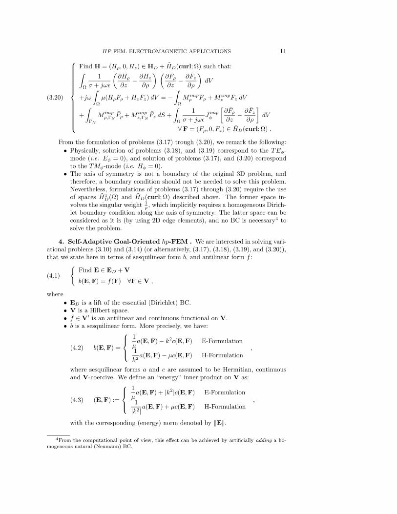
From the formulation of problems (3.17) trough (3.20), we remark the following:
• Physically, solution of problems (3.18), and (3.19) correspond to the TEφ-mode (i.e. Eφ = 0), and solution of problems (3.17), and (3.20) correspondto the TMφ-mode (i.e. Hφ = 0).
• The axis of symmetry is not a boundary of the original 3D problem, andtherefore, a boundary condition should not be needed to solve this problem.Nevertheless, formulations of problems (3.17) through (3.20) require the useof spaces H1
D(Ω) and HD(curl; Ω) described above. The former space in-volves the singular weight 1
ρ, which implicitly requires a homogeneous Dirich-
let boundary condition along the axis of symmetry. The latter space can beconsidered as it is (by using 2D edge elements), and no BC is necessary4 tosolve the problem.
4. Self-Adaptive Goal-Oriented hp-FEM . We are interested in solving vari-ational problems (3.10) and (3.14) (or alternatively, (3.17), (3.18), (3.19), and (3.20)),that we state here in terms of sesquilinear form b, and antilinear form f :
Find E ∈ ED + V
b(E,F) = f(F) ∀F ∈ V ,(4.1)
where
• ED is a lift of the essential (Dirichlet) BC.• V is a Hilbert space.• f ∈ V′ is an antilinear and continuous functional on V.• b is a sesquilinear form. More precisely, we have:
b(E,F) =
1
µa(E,F) − k2c(E,F) E-Formulation
1
k2a(E,F) − µc(E,F) H-Formulation
,(4.2)
where sesquilinear forms a and c are assumed to be Hermitian, continuousand V-coercive. We define an “energy” inner product on V as:
(E,F) :=
1
µa(E,F) + |k2|c(E,F) E-Formulation
1
|k2|a(E,F) + µc(E,F) H-Formulation,(4.3)
with the corresponding (energy) norm denoted by ‖E‖.
4From the computational point of view, this effect can be achieved by artificially adding a ho-mogeneous natural (Neumann) BC.

12 D. PARDO, L. DEMKOWICZ, C. TORRES-VERDIN, M. PASZYNSKI
4.1. Representation of the Error in the Quantity of Interest. Given anhp-FE subspace Vhp ⊂ V, we discretize (4.1) as follows:
Find Ehp ∈ ED + Vhp
b(Ehp,Fhp) = f(Fhp) ∀Fhp ∈ Vhp .(4.4)
The objective of goal-oriented adaptivity is to construct an optimal hp-grid, in thesense that it minimizes the problem size needed to achieve a given tolerance error fora given quantity of interest L, with L denoting a linear and continuous functional. Byrecalling the linearity of L, we have:
Error of interest = L(E) − L(Ehp) = L(E − Ehp) = L(e) ,(4.5)
where e = E − Ehp denotes the error function. By defining the residual rhp ∈ V′ asrhp(F) = f(F) − b(Ehp,F) = b(E − Ehp,F) = b(e,F), we look for the solution of thedual problem:
Find W ∈ V
b(F,W) = L(F) ∀F ∈ V .(4.6)
Using the Lax-Milgram theorem we conclude that problem (4.6) has a unique solutionin V. The solution W, is usually referred to as the influence function.
By discretizing (4.6) via, for example, Vhp ⊂ V, we obtain:
Find Whp ∈ Vhp
b(Fhp,Whp) = L(Fhp) ∀Fhp ∈ Vhp .(4.7)
Definition of the dual problem plus the Galerkin orthogonality for the originalproblem imply the final representation formula for the error in the quantity of interest,namely,
L(e) = b(e,W) = b(e,W − Fhp︸ ︷︷ ︸ε
) = b(e, ε) .
At this point, Fhp ∈ Vhp is arbitrary, and b(e, ε) = b(e, ε) denotes the bilinearform corresponding to the original sesquilinear form.
Notice that, in practice, the dual problem is solved not for W but for its complexconjugate W utilizing the bilinear form and not the sesquilinear form. The linearsystem of equations is factorized only once, and the extra cost of solving (4.7) reducesto only one backward and one forward substitution (if a direct solver is used).
Once the error in the quantity of interest has been determined in terms of bilinearform b, we wish to obtain a sharp upper bound for |L(e)| that depends upon the meshparameters (element size h and order of approximation p) only locally. Then, a self-adaptive algorithm intended to minimize this bound will be defined.
First, using a procedure similar to the one described in [7], we approximate Eand W with fine grid functions E h
2, p+1, Wh
2, p+1, which have been obtained by
solving the corresponding linear system of equations associated with the FE subspaceVh
2, p+1. In the remainder of this article, E and W will denote the fine grid solutions
of the direct and dual problems (E = E h
2, p+1, and W = W h
2, p+1, respectively), and
we will restrict ourselves to discrete FE spaces only.Next, we bound the error in the quantity of interest by a sum of element contri-
butions. Let bK denote a contribution from element K to sesquilinear form b. It thenfollows that
HP -FEM: ELECTROMAGNETIC APPLICATIONS 13
|L(e)| = |b(e, ε)| ≤∑
K
|bK(e, ε)| ,(4.8)
where summation over K indicates summation over elements.
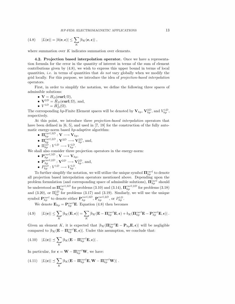
4.2. Projection based interpolation operator. Once we have a representa-tion formula for the error in the quantity of interest in terms of the sum of elementcontributions given by (4.8), we wish to express this upper bound in terms of localquantities, i.e. in terms of quantities that do not vary globally when we modify thegrid locally. For this purpose, we introduce the idea of projection-based interpolation
operators.
First, in order to simplify the notation, we define the following three spaces ofadmissible solutions:
• V = HD(curl; Ω),• V2D = HD(curl; Ω), and,• V 1D = H1
D(Ω).
The corresponding hp-Finite Element spaces will be denoted by Vhp, V2Dhp , and V 1D
hp ,respectively.
At this point, we introduce three projection-based interpolation operators thathave been defined in [6, 5], and used in [7, 18] for the construction of the fully auto-matic energy-norm based hp-adaptive algorithm:
• Πcurl,3Dhp : V −→ Vhp,
• Πcurl,2Dhp : V2D −→ V2D
hp , and,
• Π1Dhp : V 1D −→ V 1D
hp .
We shall also consider three projection operators in the energy-norm:
• Pcurl,3Dhp : V −→ Vhp,
• Pcurl,2Dhp : V2D −→ V2D
hp , and,
• P 1Dhp : V 1D −→ V 1D
hp .
To further simplify the notation, we will utilize the unique symbol Πcurlhp to denote
all projection based interpolation operators mentioned above. Depending upon theproblem formulation (and corresponding space of admissible solutions), Πcurl
hp should
be understood as Πcurl,3Dhp for problems (3.10) and (3.14), Πcurl,2D
hp for problems (3.18)
and (3.20), or Π1Dhp for problems (3.17) and (3.19). Similarly, we will use the unique
symbol Pcurlhp to denote either Pcurl,3D
hp , Pcurl,2Dhp , or P 1D
hp .
We denote Ehp = Pcurlhp E. Equation (4.8) then becomes
|L(e)| ≤∑
K
|bK(E, ε)| =∑
K
|bK(E − Πcurlhp E, ε) + bK(Πcurl
hp E − Pcurlhp E, ε)| .(4.9)
Given an element K, it is expected that |bK(Πcurlhp E − PhpE, ε)| will be negligible
compared to |bK(E − Πcurlhp E, ε)|. Under this assumption, we conclude that:
|L(e)| ¹∑
K
|bK(E − Πcurlhp E, ε)| .(4.10)
In particular, for ε = W − Πcurlhp W, we have:
|L(e)| ¹∑
K
|bK(E − Πcurlhp E,W − Πcurl
hp W)| .(4.11)
14 D. PARDO, L. DEMKOWICZ, C. TORRES-VERDIN, M. PASZYNSKI
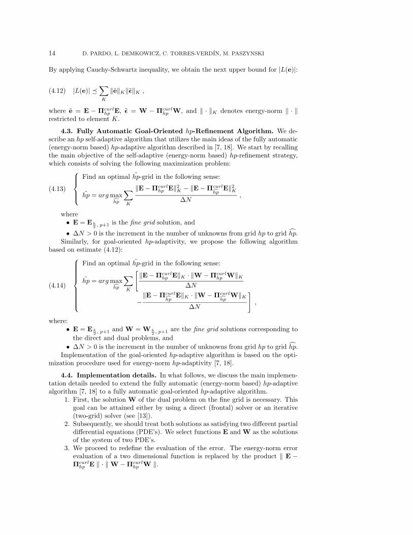
By applying Cauchy-Schwartz inequality, we obtain the next upper bound for |L(e)|:
|L(e)| ¹∑
K
‖e‖K‖ε‖K ,(4.12)
where e = E − Πcurlhp E, ε = W − Πcurl
hp W, and ‖ · ‖K denotes energy-norm ‖ · ‖restricted to element K.
4.3. Fully Automatic Goal-Oriented hp-Refinement Algorithm. We de-scribe an hp self-adaptive algorithm that utilizes the main ideas of the fully automatic(energy-norm based) hp-adaptive algorithm described in [7, 18]. We start by recallingthe main objective of the self-adaptive (energy-norm based) hp-refinement strategy,which consists of solving the following maximization problem:
Find an optimal hp-grid in the following sense:
hp = arg maxchp
∑
K
‖E − Πcurlhp E‖2
K − ‖E − Πcurlchp
E‖2K
∆N,
(4.13)
where• E = Eh
2, p+1 is the fine grid solution, and
• ∆N > 0 is the increment in the number of unknowns from grid hp to grid hp.Similarly, for goal-oriented hp-adaptivity, we propose the following algorithm
based on estimate (4.12):
Find an optimal hp-grid in the following sense:
hp = arg maxchp
∑
K
[‖E − Πcurl
hp E‖K · ‖W − Πcurlhp W‖K
∆N
−‖E − Πcurl
chpE‖K · ‖W − Πcurl
chpW‖K
∆N
],
(4.14)
where:• E = Eh
2, p+1 and W = W h
2, p+1 are the fine grid solutions corresponding to
the direct and dual problems, and
• ∆N > 0 is the increment in the number of unknowns from grid hp to grid hp.Implementation of the goal-oriented hp-adaptive algorithm is based on the opti-
mization procedure used for energy-norm hp-adaptivity [7, 18].
4.4. Implementation details. In what follows, we discuss the main implemen-tation details needed to extend the fully automatic (energy-norm based) hp-adaptivealgorithm [7, 18] to a fully automatic goal-oriented hp-adaptive algorithm.
1. First, the solution W of the dual problem on the fine grid is necessary. Thisgoal can be attained either by using a direct (frontal) solver or an iterative(two-grid) solver (see [13]).
2. Subsequently, we should treat both solutions as satisfying two different partialdifferential equations (PDE’s). We select functions E and W as the solutionsof the system of two PDE’s.
3. We proceed to redefine the evaluation of the error. The energy-norm errorevaluation of a two dimensional function is replaced by the product ‖ E −Πcurl
hp E ‖ · ‖ W − Πcurlhp W ‖.

HP -FEM: ELECTROMAGNETIC APPLICATIONS 15
4. After these simple modifications, the energy-norm based self-adaptive algo-rithm may now be utilized as a self-adaptive goal-oriented hp algorithm.
5. Numerical Results. In this Section, we apply the goal-oriented hp self-adaptive strategy described in Section 4 to simulate the response of the inductionLWD instrument operating at 2 Mhz considered in Section 2.3, using formulation(3.17) for solenoidal coils, and (3.19) for toroidal coils. Exactly the same results areobtained with formulations (3.20) and (3.18), respectively, as predicted by the theory.Thus, formulations (3.20) and (3.18) have been used as an extra verification of thesimulations, and the corresponding results have been omitted in this article to avoidduplicity.
Fig. 5.1 displays the first vertical difference of the electric field (divided by thedistance between the two receivers) for the described LWD instrument equipped withsolenoidal coils. The three curves correspond to:
1. the rock formation with no mud-filtrate invasion,2. the rock formation with a 2 Ω·m 40 cm. horizontal mud layer invading the 1
Ω·m rock formation layer, and a 5Ω·m 90cm. horizontal mud layer invadingthe 10000 Ω·m rock formation layer, and
3. the previous (mud invaded) rock formation, using a mandrel with relativemagnetic permeability of 100.
For toroidal antennas, we display in Fig. 5.2 the first vertical difference of the magneticfield (divided by the distance between the two receivers). The three displayed curvescorrespond to the three situations discussed above.
0.04 0.08 0.12 0.16 0.2−1.5
−1
−0.5
0
0.5
1
1.5
2
2.5
3
Amplitude First Vert. Diff. Electric Field (V/m2)
Ve
rtic
al P
ositio
n o
f R
ece
ivin
g A
nte
nn
a (
m)
Invasion Study
−200 −100 0 100 200−1.5
−1
−0.5
0
0.5
1
1.5
2
2.5
3
Phase (degrees)
Ve
rtic
al P
ositio
n o
f R
ece
ivin
g A
nte
nn
a (
m)
Solenoid
No Invasion0.4/0.9 m Invasion0.4/0.9m Invasion, Perm. Mandrel=100
No Invasion0.4/0.9 m Invasion0.4/0.9m Invasion, Perm. Mandrel=100
100 Ohm−m
10000 Ohm−m
1 Ohm−m
100 Ohm−m
100 Ohm−m
10000 Ohm−m
1 Ohm−m
100 Ohm−m
2 Ohm−m (0.4m) 2 Ohm−m (0.4m)
5 Ohm−m (0.9m) 5 Ohm−m (0.9m)
Fig. 5.1. LWD problem equipped with a solenoidal source. Amplitude (left panel) and phase(right panel) of the first vertical difference of the electric field (divided by the distance betweenreceivers) at the receiving coils. Results obtained with the self-adaptive goal-oriented hp-FEM. Thespatial distribution of electrical resistivity is also displayed to facilitate the physical interpretationof results.

16 D. PARDO, L. DEMKOWICZ, C. TORRES-VERDIN, M. PASZYNSKI
10−5
10−3
10−1
−1.5
−1
−0.5
0
0.5
1
1.5
2
2.5
3
Amplitude First Vert. Diff. Magnetic Field (A/m2)
Ve
rtic
al P
ositio
n o
f R
ece
ivin
g A
nte
nn
a (
m)
Invasion Study
−200 −100 0 100 200−1.5
−1
−0.5
0
0.5
1
1.5
2
2.5
3
Phase (degrees)
Ve
rtic
al P
ositio
n o
f R
ece
ivin
g A
nte
nn
a (
m)
Toroid
No Invasion0.4/0.9 m Invasion0.4/0.9m Invasion, Perm. Mandrel=100
No Invasion0.4/0.9 m Invasion0.4/0.9m Invasion, Perm. Mandrel=100
100 Ohm−m
10000 Ohm−m
1 Ohm−m
100 Ohm−m
100 Ohm−m
10000 Ohm−m
1 Ohm−m
100 Ohm−m
2 Ohm−m (0.4m) 2 Ohm−m (0.4m)
5 Ohm−m (0.9m) 5 Ohm−m (0.9m)
Fig. 5.2. LWD problem equipped with a toroidal source. Amplitude (left panel) and phase(right panel) of the first vertical difference of the magnetic field (divided by the distance betweenreceivers) at the receiving coils. Results obtained with the self-adaptive goal-oriented hp-FEM. Thespatial distribution of electrical resistivity is also displayed to facilitate the physical interpretationof results.
These results illustrate the strong dependence of the LWD response on the rockformation resistivity. We observe that solenoidal antennas are more sensitive to highlyconductive formations as well as to the electrical permeability of the mandrel, whiletoroidal antennas are more sensitive to highly resistive formations.
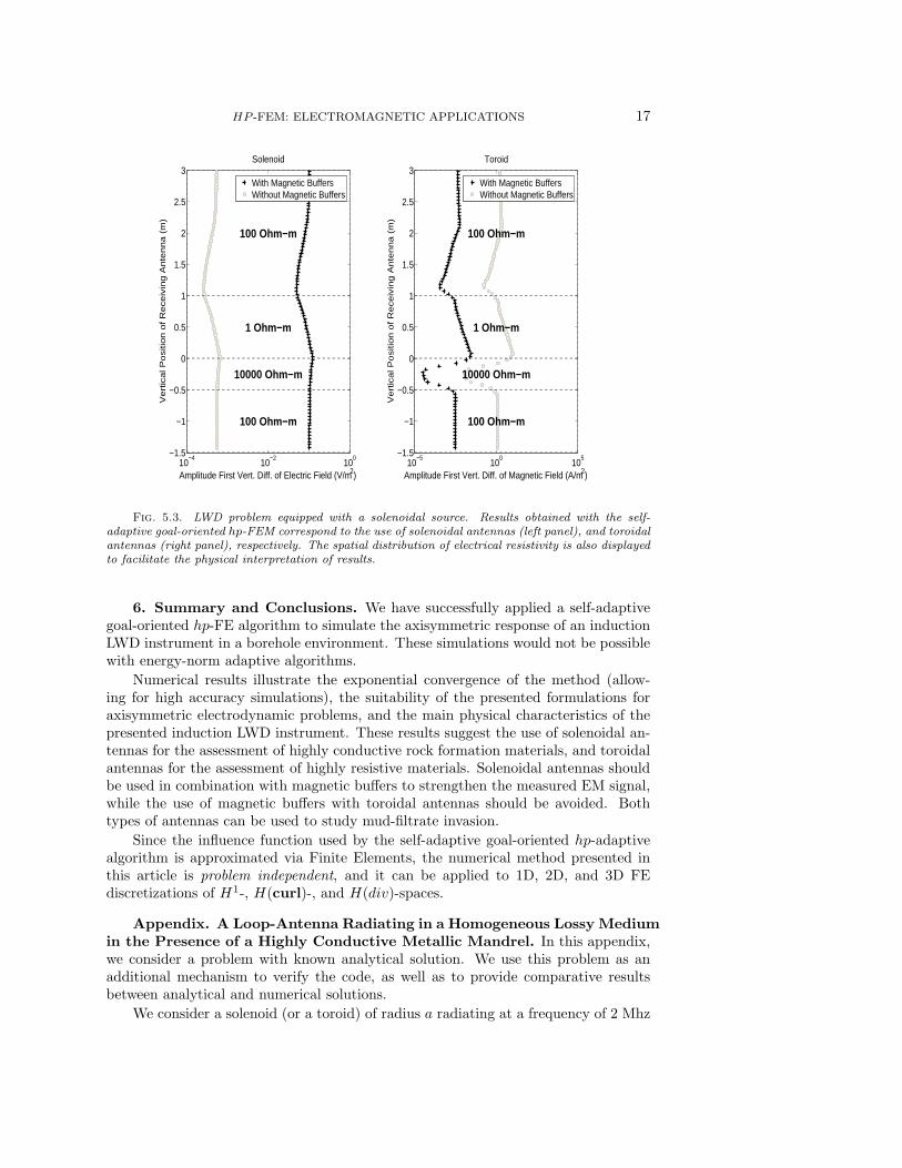
Fig. 5.3 illustrates the effect of the magnetic buffers. By removing the magneticbuffers from the logging instrument’s design, the amplitude of the received signaldecreases by a factor of up to 200 in the case of a solenoidal source. For practicalapplications, a strong signal on the receivers is desired to minimize the noise-to-signalratio. Thus, it is appropriate to use magnetic buffers in combination with solenoidalantennas. On the contrary, the use of magnetic buffers with toroidal antennas is notadvisable since they weaken the received signal. In both cases, the phase and shapeof the solution is not sensitive to the presence (or not) of magnetic buffers, and thecorresponding results have been omitted.
The exponential convergence obtained using the self-adaptive goal-oriented hp-FEM is shown in Fig. 5.4 (left panel), by considering an arbitrary fixed position ofthe logging instrument for a solenoid antenna. The final grid delivers a relative errorin the quantity of interest below 0.00001%, i.e. the first 7 significant digits of thequantity of interest are exact. In Fig. 5.4 (right panel), we display the exponentialconvergence of the energy-norm based hp-FEM. The final hp-grid delivers an energy-norm error below 0.01%. Nevertheless, the quantity of interest still contains a relativeerror above 15%.
A final goal-oriented hp-grid delivering a relative error in the quantity of interestof 0.1% is displayed in Fig. 5.5.
HP -FEM: ELECTROMAGNETIC APPLICATIONS 17
10−4
10−2
100
−1.5
−1
−0.5
0
0.5
1
1.5
2
2.5
3
Amplitude First Vert. Diff. of Electric Field (V/m2)
Ve
rtic
al P
ositio
n o
f R
ece
ivin
g A
nte
nn
a (
m)
Solenoid
−200 −100 0 100 200−1.5
−1
−0.5
0
0.5
1
1.5
2
2.5
3
Phase (degrees)
Ve
rtic
al P
ositio
n o
f R
ece
ivin
g A
nte
nn
a (
m)
With Magnetic BuffersWithout Magnetic Buffers
With Magnetic BuffersWithout Magnetic Buffers
100 Ohm−m
10000 Ohm−m
1 Ohm−m
100 Ohm−m
100 Ohm−m
10000 Ohm−m
1 Ohm−m
100 Ohm−m
10−5
100
105
−1.5
−1
−0.5
0
0.5
1
1.5
2
2.5
3
Amplitude First Vert. Diff. of Magnetic Field (A/m2)
Ve
rtic
al P
ositio
n o
f R
ece
ivin
g A
nte
nn
a (
m)
Toroid
−200 −100 0 100 200−1.5
−1
−0.5
0
0.5
1
1.5
2
2.5
3
Phase (degrees)
Ve
rtic
al P
ositio
n o
f R
ece
ivin
g A
nte
nn
a (
m)
With Magnetic BuffersWithout Magnetic Buffers
With Magnetic BuffersWithout Magnetic Buffers
100 Ohm−m
10000 Ohm−m
1 Ohm−m
100 Ohm−m
100 Ohm−m
10000 Ohm−m
1 Ohm−m
100 Ohm−m
Fig. 5.3. LWD problem equipped with a solenoidal source. Results obtained with the self-adaptive goal-oriented hp-FEM correspond to the use of solenoidal antennas (left panel), and toroidalantennas (right panel), respectively. The spatial distribution of electrical resistivity is also displayedto facilitate the physical interpretation of results.
6. Summary and Conclusions. We have successfully applied a self-adaptivegoal-oriented hp-FE algorithm to simulate the axisymmetric response of an inductionLWD instrument in a borehole environment. These simulations would not be possiblewith energy-norm adaptive algorithms.
Numerical results illustrate the exponential convergence of the method (allow-ing for high accuracy simulations), the suitability of the presented formulations foraxisymmetric electrodynamic problems, and the main physical characteristics of thepresented induction LWD instrument. These results suggest the use of solenoidal an-tennas for the assessment of highly conductive rock formation materials, and toroidalantennas for the assessment of highly resistive materials. Solenoidal antennas shouldbe used in combination with magnetic buffers to strengthen the measured EM signal,while the use of magnetic buffers with toroidal antennas should be avoided. Bothtypes of antennas can be used to study mud-filtrate invasion.
Since the influence function used by the self-adaptive goal-oriented hp-adaptivealgorithm is approximated via Finite Elements, the numerical method presented inthis article is problem independent, and it can be applied to 1D, 2D, and 3D FEdiscretizations of H1-, H(curl)-, and H(div)-spaces.
Appendix. A Loop-Antenna Radiating in a Homogeneous Lossy Mediumin the Presence of a Highly Conductive Metallic Mandrel. In this appendix,we consider a problem with known analytical solution. We use this problem as anadditional mechanism to verify the code, as well as to provide comparative resultsbetween analytical and numerical solutions.
We consider a solenoid (or a toroid) of radius a radiating at a frequency of 2 Mhz

18 D. PARDO, L. DEMKOWICZ, C. TORRES-VERDIN, M. PASZYNSKI
0 1000 8000 27000 6400010
−5
10−4
10−3
10−2
10−1
100
101
102
103
Number of Unknowns N (scale N1/3)
Re
lative
Err
or
in %
Goal−Oriented hp−Adaptivity
0 1000 8000 27000 6400010
−5
10−4
10−3
10−2
10−1
100
101
102
103
Number of Unknowns N (scale N1/3)
Re
lative
Err
or
in %
Energy−norm hp−Adaptivity
Upper bound for |L(e)|/|L(u)||L(e)|/|L(u)|
Energy−norm error|L(e)|/|L(u)|
Fig. 5.4. LWD problem equipped with a solenoidal source. Left panel: convergence behaviorobtained with the self-adaptive goal-oriented hp-FEM shows exponential convergence rates for esti-mate (4.8) (solid curve) used for optimization. The dashed curve describes the relative error in thequantity of interest. Right panel: convergence behavior obtained with the self-adaptive energy-normhp-FEM shows exponential convergence rates for the energy-norm. The dashed curve describes therelative error in the quantity of interest.
xyz
2Dhp90: A Fully automatic hp-adaptive Finite Element code2Dhp90: A Fully automatic hp-adaptive Finite Element code2Dhp90: A Fully automatic hp-adaptive Finite Element code2Dhp90: A Fully automatic hp-adaptive Finite Element code2Dhp90: A Fully automatic hp-adaptive Finite Element code2Dhp90: A Fully automatic hp-adaptive Finite Element code2Dhp90: A Fully automatic hp-adaptive Finite Element code2Dhp90: A Fully automatic hp-adaptive Finite Element code2Dhp90: A Fully automatic hp-adaptive Finite Element code2Dhp90: A Fully automatic hp-adaptive Finite Element code2Dhp90: A Fully automatic hp-adaptive Finite Element code2Dhp90: A Fully automatic hp-adaptive Finite Element code2Dhp90: A Fully automatic hp-adaptive Finite Element code2Dhp90: A Fully automatic hp-adaptive Finite Element code2Dhp90: A Fully automatic hp-adaptive Finite Element code2Dhp90: A Fully automatic hp-adaptive Finite Element code2Dhp90: A Fully automatic hp-adaptive Finite Element code2Dhp90: A Fully automatic hp-adaptive Finite Element code2Dhp90: A Fully automatic hp-adaptive Finite Element code2Dhp90: A Fully automatic hp-adaptive Finite Element code2Dhp90: A Fully automatic hp-adaptive Finite Element code2Dhp90: A Fully automatic hp-adaptive Finite Element code2Dhp90: A Fully automatic hp-adaptive Finite Element code2Dhp90: A Fully automatic hp-adaptive Finite Element code2Dhp90: A Fully automatic hp-adaptive Finite Element code2Dhp90: A Fully automatic hp-adaptive Finite Element code2Dhp90: A Fully automatic hp-adaptive Finite Element code2Dhp90: A Fully automatic hp-adaptive Finite Element code2Dhp90: A Fully automatic hp-adaptive Finite Element code2Dhp90: A Fully automatic hp-adaptive Finite Element code2Dhp90: A Fully automatic hp-adaptive Finite Element code2Dhp90: A Fully automatic hp-adaptive Finite Element code2Dhp90: A Fully automatic hp-adaptive Finite Element code2Dhp90: A Fully automatic hp-adaptive Finite Element code2Dhp90: A Fully automatic hp-adaptive Finite Element code2Dhp90: A Fully automatic hp-adaptive Finite Element code2Dhp90: A Fully automatic hp-adaptive Finite Element code2Dhp90: A Fully automatic hp-adaptive Finite Element code2Dhp90: A Fully automatic hp-adaptive Finite Element code2Dhp90: A Fully automatic hp-adaptive Finite Element code2Dhp90: A Fully automatic hp-adaptive Finite Element code2Dhp90: A Fully automatic hp-adaptive Finite Element code2Dhp90: A Fully automatic hp-adaptive Finite Element code2Dhp90: A Fully automatic hp-adaptive Finite Element code2Dhp90: A Fully automatic hp-adaptive Finite Element code2Dhp90: A Fully automatic hp-adaptive Finite Element code2Dhp90: A Fully automatic hp-adaptive Finite Element code2Dhp90: A Fully automatic hp-adaptive Finite Element code2Dhp90: A Fully automatic hp-adaptive Finite Element code2Dhp90: A Fully automatic hp-adaptive Finite Element code2Dhp90: A Fully automatic hp-adaptive Finite Element code2Dhp90: A Fully automatic hp-adaptive Finite Element code2Dhp90: A Fully automatic hp-adaptive Finite Element code2Dhp90: A Fully automatic hp-adaptive Finite Element code2Dhp90: A Fully automatic hp-adaptive Finite Element code2Dhp90: A Fully automatic hp-adaptive Finite Element code2Dhp90: A Fully automatic hp-adaptive Finite Element code2Dhp90: A Fully automatic hp-adaptive Finite Element code2Dhp90: A Fully automatic hp-adaptive Finite Element code2Dhp90: A Fully automatic hp-adaptive Finite Element code2Dhp90: A Fully automatic hp-adaptive Finite Element code2Dhp90: A Fully automatic hp-adaptive Finite Element code2Dhp90: A Fully automatic hp-adaptive Finite Element code2Dhp90: A Fully automatic hp-adaptive Finite Element code2Dhp90: A Fully automatic hp-adaptive Finite Element code2Dhp90: A Fully automatic hp-adaptive Finite Element code2Dhp90: A Fully automatic hp-adaptive Finite Element code2Dhp90: A Fully automatic hp-adaptive Finite Element code2Dhp90: A Fully automatic hp-adaptive Finite Element code2Dhp90: A Fully automatic hp-adaptive Finite Element code2Dhp90: A Fully automatic hp-adaptive Finite Element code2Dhp90: A Fully automatic hp-adaptive Finite Element code2Dhp90: A Fully automatic hp-adaptive Finite Element code2Dhp90: A Fully automatic hp-adaptive Finite Element code2Dhp90: A Fully automatic hp-adaptive Finite Element code2Dhp90: A Fully automatic hp-adaptive Finite Element code2Dhp90: A Fully automatic hp-adaptive Finite Element code2Dhp90: A Fully automatic hp-adaptive Finite Element code2Dhp90: A Fully automatic hp-adaptive Finite Element code2Dhp90: A Fully automatic hp-adaptive Finite Element code2Dhp90: A Fully automatic hp-adaptive Finite Element code2Dhp90: A Fully automatic hp-adaptive Finite Element code2Dhp90: A Fully automatic hp-adaptive Finite Element code2Dhp90: A Fully automatic hp-adaptive Finite Element code2Dhp90: A Fully automatic hp-adaptive Finite Element code2Dhp90: A Fully automatic hp-adaptive Finite Element code2Dhp90: A Fully automatic hp-adaptive Finite Element code2Dhp90: A Fully automatic hp-adaptive Finite Element code2Dhp90: A Fully automatic hp-adaptive Finite Element code2Dhp90: A Fully automatic hp-adaptive Finite Element code2Dhp90: A Fully automatic hp-adaptive Finite Element code2Dhp90: A Fully automatic hp-adaptive Finite Element code2Dhp90: A Fully automatic hp-adaptive Finite Element code2Dhp90: A Fully automatic hp-adaptive Finite Element code2Dhp90: A Fully automatic hp-adaptive Finite Element code2Dhp90: A Fully automatic hp-adaptive Finite Element code2Dhp90: A Fully automatic hp-adaptive Finite Element code2Dhp90: A Fully automatic hp-adaptive Finite Element code2Dhp90: A Fully automatic hp-adaptive Finite Element code2Dhp90: A Fully automatic hp-adaptive Finite Element code2Dhp90: A Fully automatic hp-adaptive Finite Element code2Dhp90: A Fully automatic hp-adaptive Finite Element code2Dhp90: A Fully automatic hp-adaptive Finite Element code2Dhp90: A Fully automatic hp-adaptive Finite Element code2Dhp90: A Fully automatic hp-adaptive Finite Element code2Dhp90: A Fully automatic hp-adaptive Finite Element code2Dhp90: A Fully automatic hp-adaptive Finite Element code2Dhp90: A Fully automatic hp-adaptive Finite Element code2Dhp90: A Fully automatic hp-adaptive Finite Element code2Dhp90: A Fully automatic hp-adaptive Finite Element code2Dhp90: A Fully automatic hp-adaptive Finite Element code2Dhp90: A Fully automatic hp-adaptive Finite Element code2Dhp90: A Fully automatic hp-adaptive Finite Element code2Dhp90: A Fully automatic hp-adaptive Finite Element code2Dhp90: A Fully automatic hp-adaptive Finite Element code2Dhp90: A Fully automatic hp-adaptive Finite Element code2Dhp90: A Fully automatic hp-adaptive Finite Element code2Dhp90: A Fully automatic hp-adaptive Finite Element code2Dhp90: A Fully automatic hp-adaptive Finite Element code2Dhp90: A Fully automatic hp-adaptive Finite Element code2Dhp90: A Fully automatic hp-adaptive Finite Element code2Dhp90: A Fully automatic hp-adaptive Finite Element code2Dhp90: A Fully automatic hp-adaptive Finite Element code2Dhp90: A Fully automatic hp-adaptive Finite Element code2Dhp90: A Fully automatic hp-adaptive Finite Element code2Dhp90: A Fully automatic hp-adaptive Finite Element code2Dhp90: A Fully automatic hp-adaptive Finite Element code2Dhp90: A Fully automatic hp-adaptive Finite Element code2Dhp90: A Fully automatic hp-adaptive Finite Element code2Dhp90: A Fully automatic hp-adaptive Finite Element code2Dhp90: A Fully automatic hp-adaptive Finite Element code2Dhp90: A Fully automatic hp-adaptive Finite Element code2Dhp90: A Fully automatic hp-adaptive Finite Element code2Dhp90: A Fully automatic hp-adaptive Finite Element code2Dhp90: A Fully automatic hp-adaptive Finite Element code2Dhp90: A Fully automatic hp-adaptive Finite Element code2Dhp90: A Fully automatic hp-adaptive Finite Element code2Dhp90: A Fully automatic hp-adaptive Finite Element code2Dhp90: A Fully automatic hp-adaptive Finite Element code2Dhp90: A Fully automatic hp-adaptive Finite Element code2Dhp90: A Fully automatic hp-adaptive Finite Element code2Dhp90: A Fully automatic hp-adaptive Finite Element code2Dhp90: A Fully automatic hp-adaptive Finite Element code2Dhp90: A Fully automatic hp-adaptive Finite Element code2Dhp90: A Fully automatic hp-adaptive Finite Element code2Dhp90: A Fully automatic hp-adaptive Finite Element code2Dhp90: A Fully automatic hp-adaptive Finite Element code2Dhp90: A Fully automatic hp-adaptive Finite Element code2Dhp90: A Fully automatic hp-adaptive Finite Element code2Dhp90: A Fully automatic hp-adaptive Finite Element code2Dhp90: A Fully automatic hp-adaptive Finite Element code2Dhp90: A Fully automatic hp-adaptive Finite Element code2Dhp90: A Fully automatic hp-adaptive Finite Element code2Dhp90: A Fully automatic hp-adaptive Finite Element code2Dhp90: A Fully automatic hp-adaptive Finite Element code2Dhp90: A Fully automatic hp-adaptive Finite Element code2Dhp90: A Fully automatic hp-adaptive Finite Element code2Dhp90: A Fully automatic hp-adaptive Finite Element code2Dhp90: A Fully automatic hp-adaptive Finite Element code2Dhp90: A Fully automatic hp-adaptive Finite Element code2Dhp90: A Fully automatic hp-adaptive Finite Element code2Dhp90: A Fully automatic hp-adaptive Finite Element code2Dhp90: A Fully automatic hp-adaptive Finite Element code2Dhp90: A Fully automatic hp-adaptive Finite Element code2Dhp90: A Fully automatic hp-adaptive Finite Element code2Dhp90: A Fully automatic hp-adaptive Finite Element code2Dhp90: A Fully automatic hp-adaptive Finite Element code2Dhp90: A Fully automatic hp-adaptive Finite Element code2Dhp90: A Fully automatic hp-adaptive Finite Element code2Dhp90: A Fully automatic hp-adaptive Finite Element code2Dhp90: A Fully automatic hp-adaptive Finite Element code2Dhp90: A Fully automatic hp-adaptive Finite Element code2Dhp90: A Fully automatic hp-adaptive Finite Element code2Dhp90: A Fully automatic hp-adaptive Finite Element code2Dhp90: A Fully automatic hp-adaptive Finite Element code2Dhp90: A Fully automatic hp-adaptive Finite Element code2Dhp90: A Fully automatic hp-adaptive Finite Element code2Dhp90: A Fully automatic hp-adaptive Finite Element code2Dhp90: A Fully automatic hp-adaptive Finite Element code2Dhp90: A Fully automatic hp-adaptive Finite Element code2Dhp90: A Fully automatic hp-adaptive Finite Element code2Dhp90: A Fully automatic hp-adaptive Finite Element code2Dhp90: A Fully automatic hp-adaptive Finite Element code2Dhp90: A Fully automatic hp-adaptive Finite Element code2Dhp90: A Fully automatic hp-adaptive Finite Element code2Dhp90: A Fully automatic hp-adaptive Finite Element code2Dhp90: A Fully automatic hp-adaptive Finite Element code2Dhp90: A Fully automatic hp-adaptive Finite Element code2Dhp90: A Fully automatic hp-adaptive Finite Element code2Dhp90: A Fully automatic hp-adaptive Finite Element code2Dhp90: A Fully automatic hp-adaptive Finite Element code2Dhp90: A Fully automatic hp-adaptive Finite Element code2Dhp90: A Fully automatic hp-adaptive Finite Element code2Dhp90: A Fully automatic hp-adaptive Finite Element code2Dhp90: A Fully automatic hp-adaptive Finite Element code2Dhp90: A Fully automatic hp-adaptive Finite Element code2Dhp90: A Fully automatic hp-adaptive Finite Element code2Dhp90: A Fully automatic hp-adaptive Finite Element code2Dhp90: A Fully automatic hp-adaptive Finite Element code2Dhp90: A Fully automatic hp-adaptive Finite Element code2Dhp90: A Fully automatic hp-adaptive Finite Element code2Dhp90: A Fully automatic hp-adaptive Finite Element code2Dhp90: A Fully automatic hp-adaptive Finite Element code2Dhp90: A Fully automatic hp-adaptive Finite Element code2Dhp90: A Fully automatic hp-adaptive Finite Element code2Dhp90: A Fully automatic hp-adaptive Finite Element code2Dhp90: A Fully automatic hp-adaptive Finite Element code2Dhp90: A Fully automatic hp-adaptive Finite Element code2Dhp90: A Fully automatic hp-adaptive Finite Element code2Dhp90: A Fully automatic hp-adaptive Finite Element code2Dhp90: A Fully automatic hp-adaptive Finite Element code2Dhp90: A Fully automatic hp-adaptive Finite Element code2Dhp90: A Fully automatic hp-adaptive Finite Element code2Dhp90: A Fully automatic hp-adaptive Finite Element code2Dhp90: A Fully automatic hp-adaptive Finite Element code2Dhp90: A Fully automatic hp-adaptive Finite Element code2Dhp90: A Fully automatic hp-adaptive Finite Element code2Dhp90: A Fully automatic hp-adaptive Finite Element code2Dhp90: A Fully automatic hp-adaptive Finite Element code2Dhp90: A Fully automatic hp-adaptive Finite Element code2Dhp90: A Fully automatic hp-adaptive Finite Element code2Dhp90: A Fully automatic hp-adaptive Finite Element code2Dhp90: A Fully automatic hp-adaptive Finite Element code2Dhp90: A Fully automatic hp-adaptive Finite Element code2Dhp90: A Fully automatic hp-adaptive Finite Element code2Dhp90: A Fully automatic hp-adaptive Finite Element code2Dhp90: A Fully automatic hp-adaptive Finite Element code2Dhp90: A Fully automatic hp-adaptive Finite Element code2Dhp90: A Fully automatic hp-adaptive Finite Element code2Dhp90: A Fully automatic hp-adaptive Finite Element code2Dhp90: A Fully automatic hp-adaptive Finite Element code2Dhp90: A Fully automatic hp-adaptive Finite Element code2Dhp90: A Fully automatic hp-adaptive Finite Element code2Dhp90: A Fully automatic hp-adaptive Finite Element code2Dhp90: A Fully automatic hp-adaptive Finite Element code2Dhp90: A Fully automatic hp-adaptive Finite Element code2Dhp90: A Fully automatic hp-adaptive Finite Element code2Dhp90: A Fully automatic hp-adaptive Finite Element code2Dhp90: A Fully automatic hp-adaptive Finite Element code2Dhp90: A Fully automatic hp-adaptive Finite Element code2Dhp90: A Fully automatic hp-adaptive Finite Element code2Dhp90: A Fully automatic hp-adaptive Finite Element code2Dhp90: A Fully automatic hp-adaptive Finite Element code2Dhp90: A Fully automatic hp-adaptive Finite Element code2Dhp90: A Fully automatic hp-adaptive Finite Element code2Dhp90: A Fully automatic hp-adaptive Finite Element code2Dhp90: A Fully automatic hp-adaptive Finite Element code2Dhp90: A Fully automatic hp-adaptive Finite Element code2Dhp90: A Fully automatic hp-adaptive Finite Element code2Dhp90: A Fully automatic hp-adaptive Finite Element code2Dhp90: A Fully automatic hp-adaptive Finite Element code2Dhp90: A Fully automatic hp-adaptive Finite Element code2Dhp90: A Fully automatic hp-adaptive Finite Element code2Dhp90: A Fully automatic hp-adaptive Finite Element code2Dhp90: A Fully automatic hp-adaptive Finite Element code2Dhp90: A Fully automatic hp-adaptive Finite Element code2Dhp90: A Fully automatic hp-adaptive Finite Element code2Dhp90: A Fully automatic hp-adaptive Finite Element code2Dhp90: A Fully automatic hp-adaptive Finite Element code2Dhp90: A Fully automatic hp-adaptive Finite Element code2Dhp90: A Fully automatic hp-adaptive Finite Element code2Dhp90: A Fully automatic hp-adaptive Finite Element code2Dhp90: A Fully automatic hp-adaptive Finite Element code2Dhp90: A Fully automatic hp-adaptive Finite Element code2Dhp90: A Fully automatic hp-adaptive Finite Element code2Dhp90: A Fully automatic hp-adaptive Finite Element code2Dhp90: A Fully automatic hp-adaptive Finite Element code2Dhp90: A Fully automatic hp-adaptive Finite Element code2Dhp90: A Fully automatic hp-adaptive Finite Element code2Dhp90: A Fully automatic hp-adaptive Finite Element code2Dhp90: A Fully automatic hp-adaptive Finite Element code2Dhp90: A Fully automatic hp-adaptive Finite Element code2Dhp90: A Fully automatic hp-adaptive Finite Element code2Dhp90: A Fully automatic hp-adaptive Finite Element code2Dhp90: A Fully automatic hp-adaptive Finite Element code2Dhp90: A Fully automatic hp-adaptive Finite Element code2Dhp90: A Fully automatic hp-adaptive Finite Element code2Dhp90: A Fully automatic hp-adaptive Finite Element code2Dhp90: A Fully automatic hp-adaptive Finite Element code2Dhp90: A Fully automatic hp-adaptive Finite Element code2Dhp90: A Fully automatic hp-adaptive Finite Element code2Dhp90: A Fully automatic hp-adaptive Finite Element code2Dhp90: A Fully automatic hp-adaptive Finite Element code2Dhp90: A Fully automatic hp-adaptive Finite Element code2Dhp90: A Fully automatic hp-adaptive Finite Element code2Dhp90: A Fully automatic hp-adaptive Finite Element code2Dhp90: A Fully automatic hp-adaptive Finite Element code2Dhp90: A Fully automatic hp-adaptive Finite Element code2Dhp90: A Fully automatic hp-adaptive Finite Element code2Dhp90: A Fully automatic hp-adaptive Finite Element code2Dhp90: A Fully automatic hp-adaptive Finite Element code2Dhp90: A Fully automatic hp-adaptive Finite Element code2Dhp90: A Fully automatic hp-adaptive Finite Element code2Dhp90: A Fully automatic hp-adaptive Finite Element code2Dhp90: A Fully automatic hp-adaptive Finite Element code2Dhp90: A Fully automatic hp-adaptive Finite Element code2Dhp90: A Fully automatic hp-adaptive Finite Element code2Dhp90: A Fully automatic hp-adaptive Finite Element code2Dhp90: A Fully automatic hp-adaptive Finite Element code2Dhp90: A Fully automatic hp-adaptive Finite Element code2Dhp90: A Fully automatic hp-adaptive Finite Element code2Dhp90: A Fully automatic hp-adaptive Finite Element code2Dhp90: A Fully automatic hp-adaptive Finite Element code2Dhp90: A Fully automatic hp-adaptive Finite Element code2Dhp90: A Fully automatic hp-adaptive Finite Element code2Dhp90: A Fully automatic hp-adaptive Finite Element code2Dhp90: A Fully automatic hp-adaptive Finite Element code2Dhp90: A Fully automatic hp-adaptive Finite Element code2Dhp90: A Fully automatic hp-adaptive Finite Element code2Dhp90: A Fully automatic hp-adaptive Finite Element code2Dhp90: A Fully automatic hp-adaptive Finite Element code2Dhp90: A Fully automatic hp-adaptive Finite Element code2Dhp90: A Fully automatic hp-adaptive Finite Element code2Dhp90: A Fully automatic hp-adaptive Finite Element code2Dhp90: A Fully automatic hp-adaptive Finite Element code2Dhp90: A Fully automatic hp-adaptive Finite Element code2Dhp90: A Fully automatic hp-adaptive Finite Element code2Dhp90: A Fully automatic hp-adaptive Finite Element code2Dhp90: A Fully automatic hp-adaptive Finite Element code2Dhp90: A Fully automatic hp-adaptive Finite Element code2Dhp90: A Fully automatic hp-adaptive Finite Element code2Dhp90: A Fully automatic hp-adaptive Finite Element code2Dhp90: A Fully automatic hp-adaptive Finite Element code2Dhp90: A Fully automatic hp-adaptive Finite Element code2Dhp90: A Fully automatic hp-adaptive Finite Element code2Dhp90: A Fully automatic hp-adaptive Finite Element code2Dhp90: A Fully automatic hp-adaptive Finite Element code2Dhp90: A Fully automatic hp-adaptive Finite Element code2Dhp90: A Fully automatic hp-adaptive Finite Element code2Dhp90: A Fully automatic hp-adaptive Finite Element code2Dhp90: A Fully automatic hp-adaptive Finite Element code2Dhp90: A Fully automatic hp-adaptive Finite Element code2Dhp90: A Fully automatic hp-adaptive Finite Element code2Dhp90: A Fully automatic hp-adaptive Finite Element code2Dhp90: A Fully automatic hp-adaptive Finite Element code2Dhp90: A Fully automatic hp-adaptive Finite Element code2Dhp90: A Fully automatic hp-adaptive Finite Element code2Dhp90: A Fully automatic hp-adaptive Finite Element code2Dhp90: A Fully automatic hp-adaptive Finite Element code2Dhp90: A Fully automatic hp-adaptive Finite Element code2Dhp90: A Fully automatic hp-adaptive Finite Element code2Dhp90: A Fully automatic hp-adaptive Finite Element code2Dhp90: A Fully automatic hp-adaptive Finite Element code2Dhp90: A Fully automatic hp-adaptive Finite Element code2Dhp90: A Fully automatic hp-adaptive Finite Element code2Dhp90: A Fully automatic hp-adaptive Finite Element code2Dhp90: A Fully automatic hp-adaptive Finite Element code2Dhp90: A Fully automatic hp-adaptive Finite Element code2Dhp90: A Fully automatic hp-adaptive Finite Element code2Dhp90: A Fully automatic hp-adaptive Finite Element code2Dhp90: A Fully automatic hp-adaptive Finite Element code2Dhp90: A Fully automatic hp-adaptive Finite Element code2Dhp90: A Fully automatic hp-adaptive Finite Element code2Dhp90: A Fully automatic hp-adaptive Finite Element code2Dhp90: A Fully automatic hp-adaptive Finite Element code2Dhp90: A Fully automatic hp-adaptive Finite Element code2Dhp90: A Fully automatic hp-adaptive Finite Element code2Dhp90: A Fully automatic hp-adaptive Finite Element code2Dhp90: A Fully automatic hp-adaptive Finite Element code2Dhp90: A Fully automatic hp-adaptive Finite Element code2Dhp90: A Fully automatic hp-adaptive Finite Element code2Dhp90: A Fully automatic hp-adaptive Finite Element code2Dhp90: A Fully automatic hp-adaptive Finite Element code2Dhp90: A Fully automatic hp-adaptive Finite Element code2Dhp90: A Fully automatic hp-adaptive Finite Element code2Dhp90: A Fully automatic hp-adaptive Finite Element code2Dhp90: A Fully automatic hp-adaptive Finite Element code2Dhp90: A Fully automatic hp-adaptive Finite Element code2Dhp90: A Fully automatic hp-adaptive Finite Element code2Dhp90: A Fully automatic hp-adaptive Finite Element code2Dhp90: A Fully automatic hp-adaptive Finite Element code2Dhp90: A Fully automatic hp-adaptive Finite Element code2Dhp90: A Fully automatic hp-adaptive Finite Element code2Dhp90: A Fully automatic hp-adaptive Finite Element code2Dhp90: A Fully automatic hp-adaptive Finite Element code2Dhp90: A Fully automatic hp-adaptive Finite Element code2Dhp90: A Fully automatic hp-adaptive Finite Element code2Dhp90: A Fully automatic hp-adaptive Finite Element code2Dhp90: A Fully automatic hp-adaptive Finite Element code2Dhp90: A Fully automatic hp-adaptive Finite Element code2Dhp90: A Fully automatic hp-adaptive Finite Element code2Dhp90: A Fully automatic hp-adaptive Finite Element code2Dhp90: A Fully automatic hp-adaptive Finite Element code2Dhp90: A Fully automatic hp-adaptive Finite Element code2Dhp90: A Fully automatic hp-adaptive Finite Element code2Dhp90: A Fully automatic hp-adaptive Finite Element code2Dhp90: A Fully automatic hp-adaptive Finite Element code2Dhp90: A Fully automatic hp-adaptive Finite Element code2Dhp90: A Fully automatic hp-adaptive Finite Element code2Dhp90: A Fully automatic hp-adaptive Finite Element code2Dhp90: A Fully automatic hp-adaptive Finite Element code2Dhp90: A Fully automatic hp-adaptive Finite Element code2Dhp90: A Fully automatic hp-adaptive Finite Element code2Dhp90: A Fully automatic hp-adaptive Finite Element code2Dhp90: A Fully automatic hp-adaptive Finite Element code2Dhp90: A Fully automatic hp-adaptive Finite Element code2Dhp90: A Fully automatic hp-adaptive Finite Element code2Dhp90: A Fully automatic hp-adaptive Finite Element code2Dhp90: A Fully automatic hp-adaptive Finite Element code2Dhp90: A Fully automatic hp-adaptive Finite Element code2Dhp90: A Fully automatic hp-adaptive Finite Element code2Dhp90: A Fully automatic hp-adaptive Finite Element code2Dhp90: A Fully automatic hp-adaptive Finite Element code2Dhp90: A Fully automatic hp-adaptive Finite Element code2Dhp90: A Fully automatic hp-adaptive Finite Element code2Dhp90: A Fully automatic hp-adaptive Finite Element code2Dhp90: A Fully automatic hp-adaptive Finite Element code2Dhp90: A Fully automatic hp-adaptive Finite Element code2Dhp90: A Fully automatic hp-adaptive Finite Element code2Dhp90: A Fully automatic hp-adaptive Finite Element code2Dhp90: A Fully automatic hp-adaptive Finite Element code2Dhp90: A Fully automatic hp-adaptive Finite Element code2Dhp90: A Fully automatic hp-adaptive Finite Element code2Dhp90: A Fully automatic hp-adaptive Finite Element code2Dhp90: A Fully automatic hp-adaptive Finite Element code2Dhp90: A Fully automatic hp-adaptive Finite Element code2Dhp90: A Fully automatic hp-adaptive Finite Element code2Dhp90: A Fully automatic hp-adaptive Finite Element code2Dhp90: A Fully automatic hp-adaptive Finite Element code2Dhp90: A Fully automatic hp-adaptive Finite Element code2Dhp90: A Fully automatic hp-adaptive Finite Element code2Dhp90: A Fully automatic hp-adaptive Finite Element code2Dhp90: A Fully automatic hp-adaptive Finite Element code2Dhp90: A Fully automatic hp-adaptive Finite Element code2Dhp90: A Fully automatic hp-adaptive Finite Element code2Dhp90: A Fully automatic hp-adaptive Finite Element code2Dhp90: A Fully automatic hp-adaptive Finite Element code2Dhp90: A Fully automatic hp-adaptive Finite Element code2Dhp90: A Fully automatic hp-adaptive Finite Element code2Dhp90: A Fully automatic hp-adaptive Finite Element code2Dhp90: A Fully automatic hp-adaptive Finite Element code2Dhp90: A Fully automatic hp-adaptive Finite Element code2Dhp90: A Fully automatic hp-adaptive Finite Element code2Dhp90: A Fully automatic hp-adaptive Finite Element code2Dhp90: A Fully automatic hp-adaptive Finite Element code2Dhp90: A Fully automatic hp-adaptive Finite Element code2Dhp90: A Fully automatic hp-adaptive Finite Element code2Dhp90: A Fully automatic hp-adaptive Finite Element code2Dhp90: A Fully automatic hp-adaptive Finite Element code2Dhp90: A Fully automatic hp-adaptive Finite Element code2Dhp90: A Fully automatic hp-adaptive Finite Element code2Dhp90: A Fully automatic hp-adaptive Finite Element code2Dhp90: A Fully automatic hp-adaptive Finite Element code2Dhp90: A Fully automatic hp-adaptive Finite Element code2Dhp90: A Fully automatic hp-adaptive Finite Element code2Dhp90: A Fully automatic hp-adaptive Finite Element code2Dhp90: A Fully automatic hp-adaptive Finite Element code2Dhp90: A Fully automatic hp-adaptive Finite Element code2Dhp90: A Fully automatic hp-adaptive Finite Element code2Dhp90: A Fully automatic hp-adaptive Finite Element code2Dhp90: A Fully automatic hp-adaptive Finite Element code2Dhp90: A Fully automatic hp-adaptive Finite Element code2Dhp90: A Fully automatic hp-adaptive Finite Element code2Dhp90: A Fully automatic hp-adaptive Finite Element code2Dhp90: A Fully automatic hp-adaptive Finite Element code2Dhp90: A Fully automatic hp-adaptive Finite Element code2Dhp90: A Fully automatic hp-adaptive Finite Element code2Dhp90: A Fully automatic hp-adaptive Finite Element code2Dhp90: A Fully automatic hp-adaptive Finite Element code2Dhp90: A Fully automatic hp-adaptive Finite Element code2Dhp90: A Fully automatic hp-adaptive Finite Element code2Dhp90: A Fully automatic hp-adaptive Finite Element code2Dhp90: A Fully automatic hp-adaptive Finite Element code2Dhp90: A Fully automatic hp-adaptive Finite Element code2Dhp90: A Fully automatic hp-adaptive Finite Element code2Dhp90: A Fully automatic hp-adaptive Finite Element code2Dhp90: A Fully automatic hp-adaptive Finite Element code2Dhp90: A Fully automatic hp-adaptive Finite Element code2Dhp90: A Fully automatic hp-adaptive Finite Element code2Dhp90: A Fully automatic hp-adaptive Finite Element code2Dhp90: A Fully automatic hp-adaptive Finite Element code2Dhp90: A Fully automatic hp-adaptive Finite Element code2Dhp90: A Fully automatic hp-adaptive Finite Element code2Dhp90: A Fully automatic hp-adaptive Finite Element code2Dhp90: A Fully automatic hp-adaptive Finite Element code2Dhp90: A Fully automatic hp-adaptive Finite Element code2Dhp90: A Fully automatic hp-adaptive Finite Element code2Dhp90: A Fully automatic hp-adaptive Finite Element code2Dhp90: A Fully automatic hp-adaptive Finite Element code2Dhp90: A Fully automatic hp-adaptive Finite Element code2Dhp90: A Fully automatic hp-adaptive Finite Element code2Dhp90: A Fully automatic hp-adaptive Finite Element code2Dhp90: A Fully automatic hp-adaptive Finite Element code2Dhp90: A Fully automatic hp-adaptive Finite Element code2Dhp90: A Fully automatic hp-adaptive Finite Element code2Dhp90: A Fully automatic hp-adaptive Finite Element code2Dhp90: A Fully automatic hp-adaptive Finite Element code2Dhp90: A Fully automatic hp-adaptive Finite Element code2Dhp90: A Fully automatic hp-adaptive Finite Element code2Dhp90: A Fully automatic hp-adaptive Finite Element code2Dhp90: A Fully automatic hp-adaptive Finite Element code2Dhp90: A Fully automatic hp-adaptive Finite Element code2Dhp90: A Fully automatic hp-adaptive Finite Element code2Dhp90: A Fully automatic hp-adaptive Finite Element code2Dhp90: A Fully automatic hp-adaptive Finite Element code2Dhp90: A Fully automatic hp-adaptive Finite Element code2Dhp90: A Fully automatic hp-adaptive Finite Element code2Dhp90: A Fully automatic hp-adaptive Finite Element code2Dhp90: A Fully automatic hp-adaptive Finite Element code2Dhp90: A Fully automatic hp-adaptive Finite Element code2Dhp90: A Fully automatic hp-adaptive Finite Element code2Dhp90: A Fully automatic hp-adaptive Finite Element code2Dhp90: A Fully automatic hp-adaptive Finite Element code2Dhp90: A Fully automatic hp-adaptive Finite Element code2Dhp90: A Fully automatic hp-adaptive Finite Element code2Dhp90: A Fully automatic hp-adaptive Finite Element code2Dhp90: A Fully automatic hp-adaptive Finite Element code2Dhp90: A Fully automatic hp-adaptive Finite Element code2Dhp90: A Fully automatic hp-adaptive Finite Element code2Dhp90: A Fully automatic hp-adaptive Finite Element code2Dhp90: A Fully automatic hp-adaptive Finite Element code2Dhp90: A Fully automatic hp-adaptive Finite Element code2Dhp90: A Fully automatic hp-adaptive Finite Element code2Dhp90: A Fully automatic hp-adaptive Finite Element code2Dhp90: A Fully automatic hp-adaptive Finite Element code2Dhp90: A Fully automatic hp-adaptive Finite Element code2Dhp90: A Fully automatic hp-adaptive Finite Element code2Dhp90: A Fully automatic hp-adaptive Finite Element code2Dhp90: A Fully automatic hp-adaptive Finite Element code2Dhp90: A Fully automatic hp-adaptive Finite Element code2Dhp90: A Fully automatic hp-adaptive Finite Element code2Dhp90: A Fully automatic hp-adaptive Finite Element code2Dhp90: A Fully automatic hp-adaptive Finite Element code2Dhp90: A Fully automatic hp-adaptive Finite Element code2Dhp90: A Fully automatic hp-adaptive Finite Element code2Dhp90: A Fully automatic hp-adaptive Finite Element code2Dhp90: A Fully automatic hp-adaptive Finite Element code2Dhp90: A Fully automatic hp-adaptive Finite Element code2Dhp90: A Fully automatic hp-adaptive Finite Element code2Dhp90: A Fully automatic hp-adaptive Finite Element code2Dhp90: A Fully automatic hp-adaptive Finite Element code2Dhp90: A Fully automatic hp-adaptive Finite Element code2Dhp90: A Fully automatic hp-adaptive Finite Element code2Dhp90: A Fully automatic hp-adaptive Finite Element code2Dhp90: A Fully automatic hp-adaptive Finite Element code2Dhp90: A Fully automatic hp-adaptive Finite Element code2Dhp90: A Fully automatic hp-adaptive Finite Element code2Dhp90: A Fully automatic hp-adaptive Finite Element code2Dhp90: A Fully automatic hp-adaptive Finite Element code2Dhp90: A Fully automatic hp-adaptive Finite Element code2Dhp90: A Fully automatic hp-adaptive Finite Element code2Dhp90: A Fully automatic hp-adaptive Finite Element code2Dhp90: A Fully automatic hp-adaptive Finite Element code2Dhp90: A Fully automatic hp-adaptive Finite Element code2Dhp90: A Fully automatic hp-adaptive Finite Element code2Dhp90: A Fully automatic hp-adaptive Finite Element code2Dhp90: A Fully automatic hp-adaptive Finite Element code2Dhp90: A Fully automatic hp-adaptive Finite Element code2Dhp90: A Fully automatic hp-adaptive Finite Element code2Dhp90: A Fully automatic hp-adaptive Finite Element code2Dhp90: A Fully automatic hp-adaptive Finite Element code2Dhp90: A Fully automatic hp-adaptive Finite Element code2Dhp90: A Fully automatic hp-adaptive Finite Element code2Dhp90: A Fully automatic hp-adaptive Finite Element code2Dhp90: A Fully automatic hp-adaptive Finite Element code2Dhp90: A Fully automatic hp-adaptive Finite Element code2Dhp90: A Fully automatic hp-adaptive Finite Element code2Dhp90: A Fully automatic hp-adaptive Finite Element code2Dhp90: A Fully automatic hp-adaptive Finite Element code2Dhp90: A Fully automatic hp-adaptive Finite Element code2Dhp90: A Fully automatic hp-adaptive Finite Element code2Dhp90: A Fully automatic hp-adaptive Finite Element code2Dhp90: A Fully automatic hp-adaptive Finite Element code2Dhp90: A Fully automatic hp-adaptive Finite Element code2Dhp90: A Fully automatic hp-adaptive Finite Element code2Dhp90: A Fully automatic hp-adaptive Finite Element code2Dhp90: A Fully automatic hp-adaptive Finite Element code2Dhp90: A Fully automatic hp-adaptive Finite Element code2Dhp90: A Fully automatic hp-adaptive Finite Element code2Dhp90: A Fully automatic hp-adaptive Finite Element code2Dhp90: A Fully automatic hp-adaptive Finite Element code2Dhp90: A Fully automatic hp-adaptive Finite Element code2Dhp90: A Fully automatic hp-adaptive Finite Element code2Dhp90: A Fully automatic hp-adaptive Finite Element code2Dhp90: A Fully automatic hp-adaptive Finite Element code2Dhp90: A Fully automatic hp-adaptive Finite Element code2Dhp90: A Fully automatic hp-adaptive Finite Element code2Dhp90: A Fully automatic hp-adaptive Finite Element code2Dhp90: A Fully automatic hp-adaptive Finite Element code2Dhp90: A Fully automatic hp-adaptive Finite Element code2Dhp90: A Fully automatic hp-adaptive Finite Element code2Dhp90: A Fully automatic hp-adaptive Finite Element code2Dhp90: A Fully automatic hp-adaptive Finite Element code2Dhp90: A Fully automatic hp-adaptive Finite Element code2Dhp90: A Fully automatic hp-adaptive Finite Element code2Dhp90: A Fully automatic hp-adaptive Finite Element code2Dhp90: A Fully automatic hp-adaptive Finite Element code2Dhp90: A Fully automatic hp-adaptive Finite Element code2Dhp90: A Fully automatic hp-adaptive Finite Element code2Dhp90: A Fully automatic hp-adaptive Finite Element code2Dhp90: A Fully automatic hp-adaptive Finite Element code2Dhp90: A Fully automatic hp-adaptive Finite Element code2Dhp90: A Fully automatic hp-adaptive Finite Element code2Dhp90: A Fully automatic hp-adaptive Finite Element code2Dhp90: A Fully automatic hp-adaptive Finite Element code2Dhp90: A Fully automatic hp-adaptive Finite Element code2Dhp90: A Fully automatic hp-adaptive Finite Element code2Dhp90: A Fully automatic hp-adaptive Finite Element code2Dhp90: A Fully automatic hp-adaptive Finite Element code2Dhp90: A Fully automatic hp-adaptive Finite Element code2Dhp90: A Fully automatic hp-adaptive Finite Element code2Dhp90: A Fully automatic hp-adaptive Finite Element code2Dhp90: A Fully automatic hp-adaptive Finite Element code2Dhp90: A Fully automatic hp-adaptive Finite Element code2Dhp90: A Fully automatic hp-adaptive Finite Element code2Dhp90: A Fully automatic hp-adaptive Finite Element code2Dhp90: A Fully automatic hp-adaptive Finite Element code2Dhp90: A Fully automatic hp-adaptive Finite Element code2Dhp90: A Fully automatic hp-adaptive Finite Element code2Dhp90: A Fully automatic hp-adaptive Finite Element code2Dhp90: A Fully automatic hp-adaptive Finite Element code2Dhp90: A Fully automatic hp-adaptive Finite Element code2Dhp90: A Fully automatic hp-adaptive Finite Element code2Dhp90: A Fully automatic hp-adaptive Finite Element code2Dhp90: A Fully automatic hp-adaptive Finite Element code2Dhp90: A Fully automatic hp-adaptive Finite Element code2Dhp90: A Fully automatic hp-adaptive Finite Element code2Dhp90: A Fully automatic hp-adaptive Finite Element code2Dhp90: A Fully automatic hp-adaptive Finite Element code2Dhp90: A Fully automatic hp-adaptive Finite Element code2Dhp90: A Fully automatic hp-adaptive Finite Element code2Dhp90: A Fully automatic hp-adaptive Finite Element code2Dhp90: A Fully automatic hp-adaptive Finite Element code2Dhp90: A Fully automatic hp-adaptive Finite Element code2Dhp90: A Fully automatic hp-adaptive Finite Element code2Dhp90: A Fully automatic hp-adaptive Finite Element code2Dhp90: A Fully automatic hp-adaptive Finite Element code2Dhp90: A Fully automatic hp-adaptive Finite Element code2Dhp90: A Fully automatic hp-adaptive Finite Element code2Dhp90: A Fully automatic hp-adaptive Finite Element code2Dhp90: A Fully automatic hp-adaptive Finite Element code2Dhp90: A Fully automatic hp-adaptive Finite Element code2Dhp90: A Fully automatic hp-adaptive Finite Element code2Dhp90: A Fully automatic hp-adaptive Finite Element code2Dhp90: A Fully automatic hp-adaptive Finite Element code2Dhp90: A Fully automatic hp-adaptive Finite Element code2Dhp90: A Fully automatic hp-adaptive Finite Element code2Dhp90: A Fully automatic hp-adaptive Finite Element code2Dhp90: A Fully automatic hp-adaptive Finite Element code2Dhp90: A Fully automatic hp-adaptive Finite Element code2Dhp90: A Fully automatic hp-adaptive Finite Element code2Dhp90: A Fully automatic hp-adaptive Finite Element code2Dhp90: A Fully automatic hp-adaptive Finite Element code2Dhp90: A Fully automatic hp-adaptive Finite Element code2Dhp90: A Fully automatic hp-adaptive Finite Element code2Dhp90: A Fully automatic hp-adaptive Finite Element code2Dhp90: A Fully automatic hp-adaptive Finite Element code2Dhp90: A Fully automatic hp-adaptive Finite Element code2Dhp90: A Fully automatic hp-adaptive Finite Element code2Dhp90: A Fully automatic hp-adaptive Finite Element code2Dhp90: A Fully automatic hp-adaptive Finite Element code2Dhp90: A Fully automatic hp-adaptive Finite Element code2Dhp90: A Fully automatic hp-adaptive Finite Element code2Dhp90: A Fully automatic hp-adaptive Finite Element code2Dhp90: A Fully automatic hp-adaptive Finite Element code2Dhp90: A Fully automatic hp-adaptive Finite Element code2Dhp90: A Fully automatic hp-adaptive Finite Element code2Dhp90: A Fully automatic hp-adaptive Finite Element code2Dhp90: A Fully automatic hp-adaptive Finite Element code2Dhp90: A Fully automatic hp-adaptive Finite Element code2Dhp90: A Fully automatic hp-adaptive Finite Element code2Dhp90: A Fully automatic hp-adaptive Finite Element code2Dhp90: A Fully automatic hp-adaptive Finite Element code2Dhp90: A Fully automatic hp-adaptive Finite Element code2Dhp90: A Fully automatic hp-adaptive Finite Element code2Dhp90: A Fully automatic hp-adaptive Finite Element code2Dhp90: A Fully automatic hp-adaptive Finite Element code2Dhp90: A Fully automatic hp-adaptive Finite Element code2Dhp90: A Fully automatic hp-adaptive Finite Element code2Dhp90: A Fully automatic hp-adaptive Finite Element code2Dhp90: A Fully automatic hp-adaptive Finite Element code2Dhp90: A Fully automatic hp-adaptive Finite Element code2Dhp90: A Fully automatic hp-adaptive Finite Element code2Dhp90: A Fully automatic hp-adaptive Finite Element code2Dhp90: A Fully automatic hp-adaptive Finite Element code2Dhp90: A Fully automatic hp-adaptive Finite Element code2Dhp90: A Fully automatic hp-adaptive Finite Element code2Dhp90: A Fully automatic hp-adaptive Finite Element code2Dhp90: A Fully automatic hp-adaptive Finite Element code2Dhp90: A Fully automatic hp-adaptive Finite Element code2Dhp90: A Fully automatic hp-adaptive Finite Element code2Dhp90: A Fully automatic hp-adaptive Finite Element code2Dhp90: A Fully automatic hp-adaptive Finite Element code2Dhp90: A Fully automatic hp-adaptive Finite Element code2Dhp90: A Fully automatic hp-adaptive Finite Element code2Dhp90: A Fully automatic hp-adaptive Finite Element code2Dhp90: A Fully automatic hp-adaptive Finite Element code2Dhp90: A Fully automatic hp-adaptive Finite Element code2Dhp90: A Fully automatic hp-adaptive Finite Element code2Dhp90: A Fully automatic hp-adaptive Finite Element code2Dhp90: A Fully automatic hp-adaptive Finite Element code2Dhp90: A Fully automatic hp-adaptive Finite Element code2Dhp90: A Fully automatic hp-adaptive Finite Element code2Dhp90: A Fully automatic hp-adaptive Finite Element code2Dhp90: A Fully automatic hp-adaptive Finite Element code2Dhp90: A Fully automatic hp-adaptive Finite Element code2Dhp90: A Fully automatic hp-adaptive Finite Element code2Dhp90: A Fully automatic hp-adaptive Finite Element code2Dhp90: A Fully automatic hp-adaptive Finite Element code2Dhp90: A Fully automatic hp-adaptive Finite Element code2Dhp90: A Fully automatic hp-adaptive Finite Element code2Dhp90: A Fully automatic hp-adaptive Finite Element code2Dhp90: A Fully automatic hp-adaptive Finite Element code2Dhp90: A Fully automatic hp-adaptive Finite Element code2Dhp90: A Fully automatic hp-adaptive Finite Element code2Dhp90: A Fully automatic hp-adaptive Finite Element code2Dhp90: A Fully automatic hp-adaptive Finite Element code2Dhp90: A Fully automatic hp-adaptive Finite Element code2Dhp90: A Fully automatic hp-adaptive Finite Element code2Dhp90: A Fully automatic hp-adaptive Finite Element code2Dhp90: A Fully automatic hp-adaptive Finite Element code2Dhp90: A Fully automatic hp-adaptive Finite Element code2Dhp90: A Fully automatic hp-adaptive Finite Element code2Dhp90: A Fully automatic hp-adaptive Finite Element code2Dhp90: A Fully automatic hp-adaptive Finite Element code2Dhp90: A Fully automatic hp-adaptive Finite Element code2Dhp90: A Fully automatic hp-adaptive Finite Element code2Dhp90: A Fully automatic hp-adaptive Finite Element code2Dhp90: A Fully automatic hp-adaptive Finite Element code2Dhp90: A Fully automatic hp-adaptive Finite Element code2Dhp90: A Fully automatic hp-adaptive Finite Element code2Dhp90: A Fully automatic hp-adaptive Finite Element code2Dhp90: A Fully automatic hp-adaptive Finite Element code2Dhp90: A Fully automatic hp-adaptive Finite Element code2Dhp90: A Fully automatic hp-adaptive Finite Element code2Dhp90: A Fully automatic hp-adaptive Finite Element code2Dhp90: A Fully automatic hp-adaptive Finite Element code2Dhp90: A Fully automatic hp-adaptive Finite Element code2Dhp90: A Fully automatic hp-adaptive Finite Element code2Dhp90: A Fully automatic hp-adaptive Finite Element code2Dhp90: A Fully automatic hp-adaptive Finite Element code2Dhp90: A Fully automatic hp-adaptive Finite Element code2Dhp90: A Fully automatic hp-adaptive Finite Element code2Dhp90: A Fully automatic hp-adaptive Finite Element code2Dhp90: A Fully automatic hp-adaptive Finite Element code2Dhp90: A Fully automatic hp-adaptive Finite Element code2Dhp90: A Fully automatic hp-adaptive Finite Element code2Dhp90: A Fully automatic hp-adaptive Finite Element code2Dhp90: A Fully automatic hp-adaptive Finite Element code2Dhp90: A Fully automatic hp-adaptive Finite Element code2Dhp90: A Fully automatic hp-adaptive Finite Element code2Dhp90: A Fully automatic hp-adaptive Finite Element code2Dhp90: A Fully automatic hp-adaptive Finite Element code2Dhp90: A Fully automatic hp-adaptive Finite Element code2Dhp90: A Fully automatic hp-adaptive Finite Element code2Dhp90: A Fully automatic hp-adaptive Finite Element code2Dhp90: A Fully automatic hp-adaptive Finite Element code2Dhp90: A Fully automatic hp-adaptive Finite Element code2Dhp90: A Fully automatic hp-adaptive Finite Element code2Dhp90: A Fully automatic hp-adaptive Finite Element code2Dhp90: A Fully automatic hp-adaptive Finite Element code2Dhp90: A Fully automatic hp-adaptive Finite Element code2Dhp90: A Fully automatic hp-adaptive Finite Element code2Dhp90: A Fully automatic hp-adaptive Finite Element code2Dhp90: A Fully automatic hp-adaptive Finite Element code2Dhp90: A Fully automatic hp-adaptive Finite Element code2Dhp90: A Fully automatic hp-adaptive Finite Element code2Dhp90: A Fully automatic hp-adaptive Finite Element code2Dhp90: A Fully automatic hp-adaptive Finite Element code2Dhp90: A Fully automatic hp-adaptive Finite Element code2Dhp90: A Fully automatic hp-adaptive Finite Element code2Dhp90: A Fully automatic hp-adaptive Finite Element code2Dhp90: A Fully automatic hp-adaptive Finite Element code2Dhp90: A Fully automatic hp-adaptive Finite Element code2Dhp90: A Fully automatic hp-adaptive Finite Element code2Dhp90: A Fully automatic hp-adaptive Finite Element code2Dhp90: A Fully automatic hp-adaptive Finite Element code2Dhp90: A Fully automatic hp-adaptive Finite Element code2Dhp90: A Fully automatic hp-adaptive Finite Element code2Dhp90: A Fully automatic hp-adaptive Finite Element code2Dhp90: A Fully automatic hp-adaptive Finite Element code2Dhp90: A Fully automatic hp-adaptive Finite Element code2Dhp90: A Fully automatic hp-adaptive Finite Element code2Dhp90: A Fully automatic hp-adaptive Finite Element code2Dhp90: A Fully automatic hp-adaptive Finite Element code2Dhp90: A Fully automatic hp-adaptive Finite Element code2Dhp90: A Fully automatic hp-adaptive Finite Element code2Dhp90: A Fully automatic hp-adaptive Finite Element code2Dhp90: A Fully automatic hp-adaptive Finite Element code2Dhp90: A Fully automatic hp-adaptive Finite Element code2Dhp90: A Fully automatic hp-adaptive Finite Element code2Dhp90: A Fully automatic hp-adaptive Finite Element code2Dhp90: A Fully automatic hp-adaptive Finite Element code2Dhp90: A Fully automatic hp-adaptive Finite Element code2Dhp90: A Fully automatic hp-adaptive Finite Element code2Dhp90: A Fully automatic hp-adaptive Finite Element code2Dhp90: A Fully automatic hp-adaptive Finite Element code2Dhp90: A Fully automatic hp-adaptive Finite Element code2Dhp90: A Fully automatic hp-adaptive Finite Element code2Dhp90: A Fully automatic hp-adaptive Finite Element code2Dhp90: A Fully automatic hp-adaptive Finite Element code2Dhp90: A Fully automatic hp-adaptive Finite Element code2Dhp90: A Fully automatic hp-adaptive Finite Element code2Dhp90: A Fully automatic hp-adaptive Finite Element code2Dhp90: A Fully automatic hp-adaptive Finite Element code2Dhp90: A Fully automatic hp-adaptive Finite Element code2Dhp90: A Fully automatic hp-adaptive Finite Element code2Dhp90: A Fully automatic hp-adaptive Finite Element code2Dhp90: A Fully automatic hp-adaptive Finite Element code2Dhp90: A Fully automatic hp-adaptive Finite Element code2Dhp90: A Fully automatic hp-adaptive Finite Element code2Dhp90: A Fully automatic hp-adaptive Finite Element code2Dhp90: A Fully automatic hp-adaptive Finite Element code2Dhp90: A Fully automatic hp-adaptive Finite Element code2Dhp90: A Fully automatic hp-adaptive Finite Element code2Dhp90: A Fully automatic hp-adaptive Finite Element code2Dhp90: A Fully automatic hp-adaptive Finite Element code2Dhp90: A Fully automatic hp-adaptive Finite Element code2Dhp90: A Fully automatic hp-adaptive Finite Element code2Dhp90: A Fully automatic hp-adaptive Finite Element code2Dhp90: A Fully automatic hp-adaptive Finite Element code2Dhp90: A Fully automatic hp-adaptive Finite Element code2Dhp90: A Fully automatic hp-adaptive Finite Element code2Dhp90: A Fully automatic hp-adaptive Finite Element code2Dhp90: A Fully automatic hp-adaptive Finite Element code2Dhp90: A Fully automatic hp-adaptive Finite Element code2Dhp90: A Fully automatic hp-adaptive Finite Element code2Dhp90: A Fully automatic hp-adaptive Finite Element code2Dhp90: A Fully automatic hp-adaptive Finite Element code2Dhp90: A Fully automatic hp-adaptive Finite Element code2Dhp90: A Fully automatic hp-adaptive Finite Element code2Dhp90: A Fully automatic hp-adaptive Finite Element code2Dhp90: A Fully automatic hp-adaptive Finite Element code2Dhp90: A Fully automatic hp-adaptive Finite Element code2Dhp90: A Fully automatic hp-adaptive Finite Element code2Dhp90: A Fully automatic hp-adaptive Finite Element code2Dhp90: A Fully automatic hp-adaptive Finite Element code2Dhp90: A Fully automatic hp-adaptive Finite Element code2Dhp90: A Fully automatic hp-adaptive Finite Element code2Dhp90: A Fully automatic hp-adaptive Finite Element code2Dhp90: A Fully automatic hp-adaptive Finite Element code2Dhp90: A Fully automatic hp-adaptive Finite Element code2Dhp90: A Fully automatic hp-adaptive Finite Element code2Dhp90: A Fully automatic hp-adaptive Finite Element code2Dhp90: A Fully automatic hp-adaptive Finite Element code2Dhp90: A Fully automatic hp-adaptive Finite Element code2Dhp90: A Fully automatic hp-adaptive Finite Element code2Dhp90: A Fully automatic hp-adaptive Finite Element code2Dhp90: A Fully automatic hp-adaptive Finite Element code2Dhp90: A Fully automatic hp-adaptive Finite Element code2Dhp90: A Fully automatic hp-adaptive Finite Element code2Dhp90: A Fully automatic hp-adaptive Finite Element code2Dhp90: A Fully automatic hp-adaptive Finite Element code2Dhp90: A Fully automatic hp-adaptive Finite Element code2Dhp90: A Fully automatic hp-adaptive Finite Element code2Dhp90: A Fully automatic hp-adaptive Finite Element code2Dhp90: A Fully automatic hp-adaptive Finite Element code2Dhp90: A Fully automatic hp-adaptive Finite Element code2Dhp90: A Fully automatic hp-adaptive Finite Element code2Dhp90: A Fully automatic hp-adaptive Finite Element code2Dhp90: A Fully automatic hp-adaptive Finite Element code2Dhp90: A Fully automatic hp-adaptive Finite Element code2Dhp90: A Fully automatic hp-adaptive Finite Element code2Dhp90: A Fully automatic hp-adaptive Finite Element code2Dhp90: A Fully automatic hp-adaptive Finite Element code2Dhp90: A Fully automatic hp-adaptive Finite Element code2Dhp90: A Fully automatic hp-adaptive Finite Element code2Dhp90: A Fully automatic hp-adaptive Finite Element code2Dhp90: A Fully automatic hp-adaptive Finite Element code2Dhp90: A Fully automatic hp-adaptive Finite Element code2Dhp90: A Fully automatic hp-adaptive Finite Element code2Dhp90: A Fully automatic hp-adaptive Finite Element code2Dhp90: A Fully automatic hp-adaptive Finite Element code2Dhp90: A Fully automatic hp-adaptive Finite Element code2Dhp90: A Fully automatic hp-adaptive Finite Element code2Dhp90: A Fully automatic hp-adaptive Finite Element code2Dhp90: A Fully automatic hp-adaptive Finite Element code2Dhp90: A Fully automatic hp-adaptive Finite Element code2Dhp90: A Fully automatic hp-adaptive Finite Element code2Dhp90: A Fully automatic hp-adaptive Finite Element code2Dhp90: A Fully automatic hp-adaptive Finite Element code2Dhp90: A Fully automatic hp-adaptive Finite Element code2Dhp90: A Fully automatic hp-adaptive Finite Element code2Dhp90: A Fully automatic hp-adaptive Finite Element code2Dhp90: A Fully automatic hp-adaptive Finite Element code2Dhp90: A Fully automatic hp-adaptive Finite Element code2Dhp90: A Fully automatic hp-adaptive Finite Element code2Dhp90: A Fully automatic hp-adaptive Finite Element code2Dhp90: A Fully automatic hp-adaptive Finite Element code2Dhp90: A Fully automatic hp-adaptive Finite Element code2Dhp90: A Fully automatic hp-adaptive Finite Element code2Dhp90: A Fully automatic hp-adaptive Finite Element code2Dhp90: A Fully automatic hp-adaptive Finite Element code2Dhp90: A Fully automatic hp-adaptive Finite Element code2Dhp90: A Fully automatic hp-adaptive Finite Element code2Dhp90: A Fully automatic hp-adaptive Finite Element code2Dhp90: A Fully automatic hp-adaptive Finite Element code2Dhp90: A Fully automatic hp-adaptive Finite Element code2Dhp90: A Fully automatic hp-adaptive Finite Element code2Dhp90: A Fully automatic hp-adaptive Finite Element code2Dhp90: A Fully automatic hp-adaptive Finite Element code2Dhp90: A Fully automatic hp-adaptive Finite Element code2Dhp90: A Fully automatic hp-adaptive Finite Element code2Dhp90: A Fully automatic hp-adaptive Finite Element code2Dhp90: A Fully automatic hp-adaptive Finite Element code2Dhp90: A Fully automatic hp-adaptive Finite Element code2Dhp90: A Fully automatic hp-adaptive Finite Element code2Dhp90: A Fully automatic hp-adaptive Finite Element code2Dhp90: A Fully automatic hp-adaptive Finite Element code2Dhp90: A Fully automatic hp-adaptive Finite Element code2Dhp90: A Fully automatic hp-adaptive Finite Element code2Dhp90: A Fully automatic hp-adaptive Finite Element code2Dhp90: A Fully automatic hp-adaptive Finite Element code2Dhp90: A Fully automatic hp-adaptive Finite Element code2Dhp90: A Fully automatic hp-adaptive Finite Element code2Dhp90: A Fully automatic hp-adaptive Finite Element code2Dhp90: A Fully automatic hp-adaptive Finite Element code2Dhp90: A Fully automatic hp-adaptive Finite Element code2Dhp90: A Fully automatic hp-adaptive Finite Element code2Dhp90: A Fully automatic hp-adaptive Finite Element code2Dhp90: A Fully automatic hp-adaptive Finite Element code2Dhp90: A Fully automatic hp-adaptive Finite Element code2Dhp90: A Fully automatic hp-adaptive Finite Element code2Dhp90: A Fully automatic hp-adaptive Finite Element code2Dhp90: A Fully automatic hp-adaptive Finite Element code2Dhp90: A Fully automatic hp-adaptive Finite Element code2Dhp90: A Fully automatic hp-adaptive Finite Element code2Dhp90: A Fully automatic hp-adaptive Finite Element code2Dhp90: A Fully automatic hp-adaptive Finite Element code2Dhp90: A Fully automatic hp-adaptive Finite Element code2Dhp90: A Fully automatic hp-adaptive Finite Element code2Dhp90: A Fully automatic hp-adaptive Finite Element code2Dhp90: A Fully automatic hp-adaptive Finite Element code2Dhp90: A Fully automatic hp-adaptive Finite Element code2Dhp90: A Fully automatic hp-adaptive Finite Element code2Dhp90: A Fully automatic hp-adaptive Finite Element code2Dhp90: A Fully automatic hp-adaptive Finite Element code2Dhp90: A Fully automatic hp-adaptive Finite Element code2Dhp90: A Fully automatic hp-adaptive Finite Element code2Dhp90: A Fully automatic hp-adaptive Finite Element code2Dhp90: A Fully automatic hp-adaptive Finite Element code2Dhp90: A Fully automatic hp-adaptive Finite Element code2Dhp90: A Fully automatic hp-adaptive Finite Element code2Dhp90: A Fully automatic hp-adaptive Finite Element code2Dhp90: A Fully automatic hp-adaptive Finite Element code2Dhp90: A Fully automatic hp-adaptive Finite Element code2Dhp90: A Fully automatic hp-adaptive Finite Element code2Dhp90: A Fully automatic hp-adaptive Finite Element code2Dhp90: A Fully automatic hp-adaptive Finite Element code2Dhp90: A Fully automatic hp-adaptive Finite Element code2Dhp90: A Fully automatic hp-adaptive Finite Element code2Dhp90: A Fully automatic hp-adaptive Finite Element code2Dhp90: A Fully automatic hp-adaptive Finite Element code2Dhp90: A Fully automatic hp-adaptive Finite Element code2Dhp90: A Fully automatic hp-adaptive Finite Element code2Dhp90: A Fully automatic hp-adaptive Finite Element code2Dhp90: A Fully automatic hp-adaptive Finite Element code2Dhp90: A Fully automatic hp-adaptive Finite Element code2Dhp90: A Fully automatic hp-adaptive Finite Element code2Dhp90: A Fully automatic hp-adaptive Finite Element code2Dhp90: A Fully automatic hp-adaptive Finite Element code2Dhp90: A Fully automatic hp-adaptive Finite Element code2Dhp90: A Fully automatic hp-adaptive Finite Element code2Dhp90: A Fully automatic hp-adaptive Finite Element code2Dhp90: A Fully automatic hp-adaptive Finite Element code2Dhp90: A Fully automatic hp-adaptive Finite Element code2Dhp90: A Fully automatic hp-adaptive Finite Element code2Dhp90: A Fully automatic hp-adaptive Finite Element code2Dhp90: A Fully automatic hp-adaptive Finite Element code2Dhp90: A Fully automatic hp-adaptive Finite Element code2Dhp90: A Fully automatic hp-adaptive Finite Element code2Dhp90: A Fully automatic hp-adaptive Finite Element code2Dhp90: A Fully automatic hp-adaptive Finite Element code2Dhp90: A Fully automatic hp-adaptive Finite Element code2Dhp90: A Fully automatic hp-adaptive Finite Element code2Dhp90: A Fully automatic hp-adaptive Finite Element code2Dhp90: A Fully automatic hp-adaptive Finite Element code2Dhp90: A Fully automatic hp-adaptive Finite Element code2Dhp90: A Fully automatic hp-adaptive Finite Element code2Dhp90: A Fully automatic hp-adaptive Finite Element code2Dhp90: A Fully automatic hp-adaptive Finite Element code2Dhp90: A Fully automatic hp-adaptive Finite Element code2Dhp90: A Fully automatic hp-adaptive Finite Element code2Dhp90: A Fully automatic hp-adaptive Finite Element code2Dhp90: A Fully automatic hp-adaptive Finite Element code2Dhp90: A Fully automatic hp-adaptive Finite Element code2Dhp90: A Fully automatic hp-adaptive Finite Element code2Dhp90: A Fully automatic hp-adaptive Finite Element code2Dhp90: A Fully automatic hp-adaptive Finite Element code2Dhp90: A Fully automatic hp-adaptive Finite Element code2Dhp90: A Fully automatic hp-adaptive Finite Element code2Dhp90: A Fully automatic hp-adaptive Finite Element code2Dhp90: A Fully automatic hp-adaptive Finite Element code2Dhp90: A Fully automatic hp-adaptive Finite Element code2Dhp90: A Fully automatic hp-adaptive Finite Element code2Dhp90: A Fully automatic hp-adaptive Finite Element code2Dhp90: A Fully automatic hp-adaptive Finite Element code2Dhp90: A Fully automatic hp-adaptive Finite Element code2Dhp90: A Fully automatic hp-adaptive Finite Element code2Dhp90: A Fully automatic hp-adaptive Finite Element code2Dhp90: A Fully automatic hp-adaptive Finite Element code2Dhp90: A Fully automatic hp-adaptive Finite Element code2Dhp90: A Fully automatic hp-adaptive Finite Element code2Dhp90: A Fully automatic hp-adaptive Finite Element code2Dhp90: A Fully automatic hp-adaptive Finite Element code2Dhp90: A Fully automatic hp-adaptive Finite Element code2Dhp90: A Fully automatic hp-adaptive Finite Element code2Dhp90: A Fully automatic hp-adaptive Finite Element code2Dhp90: A Fully automatic hp-adaptive Finite Element code2Dhp90: A Fully automatic hp-adaptive Finite Element code
Transmitter −→
Receiver I −→Receiver II −→
p = 8
p = 7
p = 6
p = 5
p = 4
p = 3
p = 2
p = 1
Fig. 5.5. LWD instrument equipped with a solenoidal source. Portion (120 cm x 200 cm) ofthe final hp-grid. Different colors indicate different polynomial orders of approximation, rangingfrom 1 (light grey) to 8 (white).

HP -FEM: ELECTROMAGNETIC APPLICATIONS 19
in a homogeneous lossy medium (with resistivity equal to 1 Ω ·m), in the presence ofan infinitely large cylindrical mandrel (with resistivity equal to 10−6 Ω · m) of radiusb < a. The coil and the mandrel exhibit axial symmetry (see Fig. A.1).
z
COIL (Toroid/Solenoid)
MANDREL
b a
Fig. A.1. Geometry of a loop-antenna radiating in a homogeneous lossy medium in the presenceof a highly conductive metallic mandrel.
For a solenoidal coil located at z = 0, the resulting solution for a ≤ ρ ≤ b is givenby [10, 15]:
Eφ(ρ, z) =−ωµ
4πa
∫∞
−∞
[J1(kρa) + ΓH(1)1 (kρa)]H
(1)1 (kρρ)eikzzdkρ,(A.1)
where Γ = −J1(kρb)/H(1)1 (kρb), Jp and H
(1)p are the Bessel and Hankel functions of
the first type of order p, respectively, and kz =√
k2 − k2ρ.
For a toroidal coil located at z = 0, the resulting solution for a ≤ ρ ≤ b is givenby:
Hφ(ρ, z) =−i
4πa
∫∞
−∞
[J1(kρa) + ΓH(1)1 (kρa)]H
(1)1 (kρρ)eikzzdkρ,(A.2)
where Γ = −J0(kρb)/H(1)0 (kρb).
In figures A.2 and A.3, we display a comparison between analytical and numericalresults (obtained using the self-adaptive hp goal-oriented algorithm) for the solenoidaland toroidal coils, respectively. We selected b = 0.0254 cm, and a = 0.03048 cm. Thenumerical results accurately reproduce the analytical ones, both in terms of amplitudeand phase.
When considering a solenoid, the logging instrument response using a mandrel ofresistivity 10−5 Ω · m or a PEC mandrel are indistinguishable in terms of amplitude.A similar situation occurs for a toroid. In terms of phase, induction instrumentsequipped with solenoidal coils appear to be more sensitive to the mandrel resistivitythan those equipped with toroidal coils.
Acknowledgments. This work was financially supported by Baker-Atlas andthe Joint Industry Research Consortium on Formation Evaluation supervised by Prof.C. Torres-Verdin. We would also like to acknowledge the expertise and technical advise
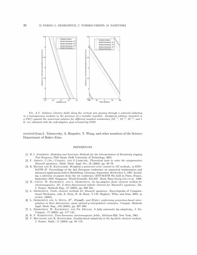
20 D. PARDO, L. DEMKOWICZ, C. TORRES-VERDIN, M. PASZYNSKI
10−8
10−6
10−4
10−2
100
0.5
1
1.5
2
2.5
3
3.5
Amplitude (V/m)
Dis
tan
ce in
z−
axi
s fr
om
tra
nsm
itte
r to
re
ceiv
er
(in
m)
−180 −90 0 90 1800.5
1
1.5
2
2.5
3
3.5
Phase (degrees)
Dis
tan
ce in
z−
axi
s fr
om
tra
nsm
itte
r to
re
ceiv
er
(in
m)
Analytical solution
Mandrel Resisitivity: 10−7
Mandrel Resisitivity: 10−5
Mandrel Resisitivity: 10−3
Mandrel Resisitivity: 1
Analytical solution
Mandrel Resisitivity: 10−7
Mandrel Resisitivity: 10−5
Mandrel Resisitivity: 10−3
Mandrel Resisitivity: 1
Fig. A.2. Solution (electric field) along the vertical axis passing through a solenoid radiatingin a homogeneous medium in the presence of a metallic mandrel. Analytical solution (mandrel isa PEC) against the numerical solution for different mandrel resistivities (10−7, 10−5, 10−3, and 1Ω ·m) obtained with the self-adaptive goal oriented hp-FEM.
received from L. Tabarovsky, A. Bespalov, T. Wang, and other members of the ScienceDepartment of Baker-Atlas.
REFERENCES
[1] B. I. Anderson, Modeling and Inversion Methods for the Interpretation of Resistivity LoggingTool Response, PhD thesis, Delft University of Technology, 2001.
[2] F. Assous, C.(Jr.) Ciarlet, and S Labrunie, Theoretical tools to solve the axisymmetricMaxwell equations., Math. Meth. Appl. Sci., 25 (2002), pp. 49–78.
[3] R. Becker and R. Rannacher, Weighted a posteriori error control in FE methods., in ENU-MATH 97. Proceedings of the 2nd European conference on numerical mathematics andadvanced applications held in Heidelberg, Germany, September 28-October 3, 1997. Includ-ing a selection of papers from the 1st conference (ENUMATH 95) held in Paris, France,September 1995. Singapore: World Scientific. 621-637 , Bock, Hans Georg (ed.) et al., 1998.
[4] W. Cecot, W. Rachowicz, and L. Demkowicz, An hp-adaptive finite element method forelectromagnetics. III: A three-dimensional infinite element for Maxwell’s equations., Int.J. Numer. Methods Eng., 57 (2003), pp. 899–921.
[5] L. Demkowicz, Finite element methods for Maxwell equations., Encyclopedia of Computa-tional Mechanics, (eds. E. Stein, R. de Borst, T.J.R. Hughes), Wiley and Sons, 2003, inreview, (2003).
[6] L. Demkowicz and A. Buffa, H1, H(curl), and H(div) conforming projection-based inter-polation in three dimensions: quasi optimal p-interpolation estimates., Comput. MethodsAppl. Mech. Eng., 194 (2005), pp. 267–296.
[7] L. Demkowicz, W. Rachowicz, and Ph. Devloo, A fully automatic hp-adaptivity., J. Sci.Comput., 17 (2002), pp. 117–142.
[8] R. F. Harrington, Time-harmonic electromagnetic fields., McGraw-Hill, New York, 1961.[9] V. Heuveline and R. Rannacher, Duality-based adaptivity in the hp-finite element method.,
J. Numer. Math., 11 (2003), pp. 95–113.

HP -FEM: ELECTROMAGNETIC APPLICATIONS 21
10−10
10−5
100
105
0.5
1
1.5
2
2.5
3
3.5
Amplitude (A/m)
Dis
tan
ce in
z−
axi
s fr
om
tra
nsm
itte
r to
re
ceiv
er
(in
m)
Analytical solution
Mandrel Resisitivity: 10−7
Mandrel Resisitivity: 10−5
Mandrel Resisitivity: 10−3
Mandrel Resisitivity: 1
−180 −90 0 90 1800.5
1
1.5
2
2.5
3
3.5
Phase (degrees)
Dis
tan
ce in
z−
axi
s fr
om
tra
nsm
itte
r to
re
ceiv
er
(in
m)
Analytical solution
Mandrel Resisitivity: 10−7
Mandrel Resisitivity: 10−5
Mandrel Resisitivity: 10−3
Mandrel Resisitivity: 1
Fig. A.3. Solution (magnetic field) along a vertical axis passing through a toroid radiating ina homogeneous medium in the presence of a metallic mandrel. Analytical solution (mandrel is aPEC) against the numerical solution for different mandrel resistivities (10−7, 10−5, 10−3, and 1Ω ·m) obtained with the self-adaptive goal oriented hp-FEM.
[10] J. R. Lovell, Finite Element Methods in Resistivity Logging, PhD thesis, Delft University ofTechnology, 1993.
[11] J.T. Oden and S. Prudhomme, Goal-oriented error estimation and adaptivity for the finiteelement method., Comput. Math. Appl., 41 (2001), pp. 735–756.
[12] M. Paraschivoiu and A. T. Patera, A hierarchical duality approach to bounds for the outputsof partial differential equations., Comput. Methods Appl. Mech. Eng., 158 (1998), pp. 389–407.
[13] D. Pardo, Integration of hp-adaptivity with a two grid solver: applications to electromagnet-ics., PhD thesis, The University of Texas at Austin, April 2004.
[14] D. Pardo, L. Demkowicz, and C. Torres-Verdin, A Goal Oriented hp-Adaptive FiniteElement Method with Electromagnetic Applications. Part I: Electrostatics., ICES Report04-57. Submitted to Int. J. Numer. Methods Eng., 0 (2005), p. 0.
[15] M. Paszynski, L. Demkowicz, and D. Pardo, Verification of Goal-Oriented hp-Adaptivity.,ICES Report 05-06, (2005).
[16] C. R. Paul and S. A. Nasar, Introduction to Electromagnetic Fields, McGraw-Hill, New York,1982.
[17] S. Prudhomme and J.T. Oden, On goal-oriented error estimation for elliptic problems: appli-cation to the control of pointwise errors., Comput. Methods Appl. Mech. Eng., 176 (1999),pp. 313–331.
[18] W. Rachowicz, D. Pardo, and L. Demkowicz, Fully automatic hp-adaptivity in three di-mensions., Tech. Report 04-22, ICES Report, 2004.
[19] R. Rannacher and F.T. Suttmeier, A posteriori error control in finite element methods viaduality techniques: application to perfect plasticity., Comput. Mech., 21 (1998), pp. 123–133.
[20] P. Solin and L. Demkowicz, Goal-oriented hp-adaptivity for elliptic problems., Comput.Methods Appl. Mech. Eng., 193 (2004), pp. 449–468.
[21] J. Van Bladel, Singular Electromagnetic Fields and Sources., Oxford University Press., NewYork, 1991.
[22] T. Wang and J. Signorelli, Finite-difference Modeling of Electromagnetic Tool Response forLogging While Drilling., Geophysics, 69 (2004), pp. 152–160.