Institutionen för systemteknik Department of Electrical Engineering

Examensarbete

Simulation of Heat Recovery Steam Generator in a Combined Cycle Power Plant

Examensarbete utfört i Modellbygge och Simulering vid Tekniska högskolan vid Linköpings universitet

av

Kristofer Horkeby

LiTH-ISY-EX--12/4548--SE

Linköping 2012

Simulation of Heat Recovery Steam Generator in a Combined Cycle Power Plant

Examensarbete utfört i Modellbygge och Simulering

vid Tekniska högskolan i Linköping av

Kristofer Horkeby

LiTH-ISY-EX--12/4548--SE

Supervisors:

Åke Kinnander, Siemens Industrial Turbomachinery AB

Sina Khoshfetrat Pakazad, Linköpings universitet

Examiner:

Torkel Glad, Linköpings universitet

Linköping, 27 Februari, 2012

Presentation Date 2012-02-27 Publishing Date (Electronic version) 2012-03-05

Department and Division Department of Electrical Engineering

URL, Electronic Version http://www.ep.liu.se

Publication Title Simulation of Heat Recovery Steam Generator in a Combined Cycle Power Plant Author(s) Kristofer Horkeby

Abstract This thesis covers the modelling of a Heat Recovery Steam Generator (HRSG) in a Combined Cycle Power Plant (CCPP). This kind of power plant has become more and more utilized because of its high efficiency and low emissions. The HRSG plays a central role in the generation of steam using the exhaust heat from the gas turbine. The purpose of the thesis was to develop efficient dynamic models for the physical components in the HRSG using the modelling and simulation software Dymola. The models are then to be used for simulations of a complete CCPP. The main application is to use the complete model to introduce various disturbances and study their consequences in the different components in the CCPP by analyzing the simulation results. The thesis is a part of an ongoing development process for the dynamic simulation capabilities offered by the Solution department at SIT AB. First, there is a theoretical explanation of the CCPP components and control system included in the scope of this thesis. Then the development method is described and the top-down approach that was used is explained. The structure and equations used are reported for each of the developed models and a functional description is given. In order to ensure that the HRSG model would function in a complete CCPP model, adaptations were made and tuning was performed on the existing surrounding component models in the CCPP. Static verifications of the models are performed by comparison to Siemens in-house software for static calculations. Dynamic verification was partially done, but work remains to guarantee the validity in a wide operating range. As a result of this thesis efficient models for the drum boiler and its control system have been developed. An operational model of a complete CCPP has been built. This was done integrating the developed models during the work with this thesis together with adaptations of already developed models. Steady state for the CCPP model is achieved during simulation and various disturbances can then be introduced and studied. Simulation time for a typical test case is longer than the time limit that has been set, mainly because of the gas turbine model. When using linear functions to approximate the gas turbine start-up curves instead, the simulation finishes within the set simulation time limit of 5 minutes for a typical test case.

Keywords Modelling and Simulation, Control System, Combined-Cycle Power Plant, Heat Recovery Steam Generator, Dymola, Modelica, Siemens

Abstract This thesis covers the modelling of a Heat Recovery Steam Generator (HRSG) in a Combined Cycle Power Plant (CCPP). This kind of power plant has become more and more utilized because of its high efficiency and low emissions. The HRSG plays a central role in the generation of steam using the exhaust heat from the gas turbine. The purpose of the thesis was to develop efficient dynamic models for the physical components in the HRSG using the modelling and simulation software Dymola. The models are then to be used for simulations of a complete CCPP. The main application is to use the complete model to introduce various disturbances and study their consequences in the different components in the CCPP by analyzing the simulation results. The thesis is a part of an ongoing development process for the dynamic simulation capabilities offered by the Solution department at SIT AB. First, there is a theoretical explanation of the CCPP components and control system included in the scope of this thesis. Then the development method is described and the top-down approach that was used is explained. The structure and equations used are reported for each of the developed models and a functional description is given. In order to ensure that the HRSG model would function in a complete CCPP model, adaptations were made and tuning was performed on the existing surrounding component models in the CCPP. Static verifications of the models are performed by comparison to Siemens in-house software for static calculations. Dynamic verification was partially done, but work remains to guarantee the validity in a wide operating range. As a result of this thesis efficient models for the drum boiler and its control system have been developed. An operational model of a complete CCPP has been built. This was done integrating the developed models during the work with this thesis together with adaptations of already developed models. Steady state for the CCPP model is achieved during simulation and various disturbances can then be introduced and studied. Simulation time for a typical test case is longer than the time limit that has been set, mainly because of the gas turbine model. When using linear functions to approximate the gas turbine start-up curves instead, the simulation finishes within the set simulation time limit of 5 minutes for a typical test case.

Sammanfattning Det här examensarbetet beskriver modelleringen av en avgaspanna i ett kombikraftverk. Kombikraftverk har blivit allt vanligare på grund av den höga effektivitet och låga utsläppshalter som lösningen erbjuder. Avgaspannan spelar en central roll vid produktionen av ånga med hjälp av värmen från gasturbinens avgaser. Syftet med det här examensarbetet var att utveckla effektiva dynamiska modeller för ångpannans komponenter i simulerings- och modelleringsmjukvaran Dymola. Modellerna används sedan för simuleringar av ett komplett kombikraftverk. Det huvudsakliga användningsområdet för den kompletta modellen är att introducera och studera effekten av olika störningar och studera dess effekter i kraftverkets olika delar genom analys av simuleringsresultat. Examensarbetet utgör en del i ett pågående utvecklingsprojekt för de dynamiska simuleringsmöjligheter som erbjuds av anläggningssektorn på SIT AB.

Först ges en teoretisk bakgrund för kombikraftverket och dess ingående komponenter som ingått i ramen för examensarbetet. Sen beskrivs utvecklingsmetoden och top-down filosofin som användes i modelleringsarbetet. Modellernas implementerade struktur och använda ekvationer redovisas sedan för varje utvecklad modell. Sedan ges en funktionell beskrivning. Statisk verifiering av modellerna genomförs sedan med hjälp av jämförelse med Siemens standardprogram för statiska beräkningar. Den dynamiska verifieringen är delvis gjord, men arbete kvarstår för att garantera validitet i ett stort arbetsområde. Genom arbetet med detta examensarbete har effektiva modeller för ångpannan och dess styrsystem utvecklats. En operativ modell av en komplett CCPP har utvecklats. Detta gjordes genom att integrera de modeller som utvecklats under examensarbetet tillsammans med anpassningar av redan utvecklade modeller. Kombikraftverkmodellen uppnår ett stabilt tillstånd under simulering, och från detta tillstånd kan olika störningar sedan införas och dess effekter på systemet studeras. Simuleringstiden för ett typiskt testfall är längre än den uppsatta tidsgränsen, främst på grund av en något långsam gasturbinmodell. När kurvan som beskriver gasturbinens avgasflöde från start istället approximerats med linjära funktioner så klaras kravet på simuleringstiden, som är 5 minuter för ett typiskt testfall.

ii

Acknowledgement Firstly, I would like to thank Åke Kinnander, my supervisor at SIT AB, for his commitment and support throughout the work with this thesis. His guidance and our interesting discussions have been invaluable to me. Secondly, I would also like to express my gratitude towards my supervisor at ISY, Sina Khoshfetrat Pakazad for his help and encouraging remarks throughout the work. Finally, I would like to thank the whole department at SIT AB for their help and I would also like to thank my opponent Niklas Ekvall. Finspång, January 2012 Kristofer Horkeby

iii

iv

Table of Contents 1 INTRODUCTION............................................................................................................ 1

1.1 BACKGROUND ............................................................................................................... 2 1.2 PURPOSE........................................................................................................................ 3 1.3 COURSE OF ACTION....................................................................................................... 3 1.4 LIMITATIONS ................................................................................................................. 4 1.5 OUTLINE........................................................................................................................ 5

2 METHOD.......................................................................................................................... 7 2.1 STEPWISE METHOD FOR MODEL DEVELOPMENT........................................................... 7

3 THE COMBINED CYCLE POWER PLANT AND ITS COMPONENTS ............. 10 3.1 GENERAL DESCRIPTION OF THERMODYNAMIC CYCLES............................................... 10 3.2 GENERAL DESCRIPTION OF A HEAT EXCHANGER ........................................................ 13 3.3 THE COMBINED CYCLE POWER PLANT........................................................................ 13 3.4 THE HEAT RECOVERY STEAM GENERATOR................................................................. 15 3.5 THE FEED WATER SYSTEM.......................................................................................... 23 3.6 THE GAS TURBINE....................................................................................................... 23 3.7 THE STEAM TURBINE .................................................................................................. 24 3.8 THE CONDENSER ......................................................................................................... 25

4 THE MODELS............................................................................................................... 27 4.1 SIMPLE MODEL OF A HEAT EXCHANGER ..................................................................... 27 4.2 THE HEAT RECOVERY STEAM GENERATOR MODEL.................................................... 29 4.3 THE FEED WATER SYSTEM.......................................................................................... 50 4.4 THE STEAM TURBINE INLET PRESSURE CONTROLLER MODEL .................................... 52 4.5 ADAPTATIONS OF OTHER MODELS .............................................................................. 52 4.6 THE COMBINED CYCLE POWER PLANT MODEL........................................................... 53

5 TESTING AND VERIFICATION ............................................................................... 56 5.1 VERIFICATION OF HRSG MODEL ................................................................................ 56 5.2 TEST OF COMPLETE CCPP MODEL.............................................................................. 78

6 DISCUSSION ................................................................................................................. 79 6.1 DISCUSSION OF MODEL DEVELOPMENT METHOD ....................................................... 79

7 CONCLUSIONS AND FUTURE WORK ................................................................... 82 7.1 CONCLUSIONS ............................................................................................................. 82 7.2 FUTURE WORK ............................................................................................................ 82

BIBLIOGRAPHY .................................................................................................................. 84 REFERENCES - FIGURES......................................................................................................... 85

APPENDIX

v

Figures and Tables Figures

Figure 1: The Brayton cycle explained by schematics, a P-v diagram and a T-s diagram ..........10 Figure 2: The components in an ideal Rankine cycle ...................................................................11 Figure 3: A T-s diagram of the ideal Rankine cycle .....................................................................12 Figure 4: A model of a shell and tube heat exchanger, a kind of heat exchanger that is common in industrial applications ..............................................................................................................13 Figure 5: Flow diagram for a common CCPP configuration. The two cycles forming the combined cycle configuration are also indicated in the picture ...................................................14 Figure 6: A 3D illustration of a Siemens turn key solution of a CCPP ........................................15 Figure 7: A detailed illustration of the components, the inputs and the outputs of a typical HRSG.......................................................................................................................................................16 Figure 8: The main flow schematics of a single-pressure level drum boiler type HRSG .............17 Figure 9: The figure explains the relationship between exhaust gas temperature and the water/steam temperatures in respective sub component in the HRSG..........................................17 Figure 10: A schematic of the forced circulation drum boiler .....................................................19 Figure 11: Schematics of the system for a three-element level control of the drum boiler ..........22 Figure 12: Schematics of the system for a two-element level control of the drum boiler.............22 Figure 13: A 3D illustration of the SGT-750. It is the machine most recently developed by SIT in Finspång with a power output of 37 MW ......................................................................................24 Figure 14: The SST-600 steam turbine is constructed at a Siemens site in Germany ..................25 Figure 15: A water cooled condenser that is to be installed on site .............................................26 Figure 16: The counter current heat exchanger model used in the economizer model. Heat from the gas side is transferred to the water side..................................................................................28 Figure 17: The model of the HRSG and its controllers. The surroundings of the model are described with the black text in the figure.....................................................................................30 Figure 18: The drum boiler model including heat exchange modelling for the risers, the drum level controller, inlet and outlet valves, sensors for pressure, mass flows and temperatures, and connectors to water/steam and gas flows......................................................................................31 Figure 19: The drum boiler model shown in the icon layer. Connectors to the economizer, the superheater, heat to the risers and drum level measurement are marked in the figure................34 Figure 20: The diagram layer of the drum boiler components in Dymola. The components are the drum, the downcomers, the risers and the circulation pump ..................................................34 Figure 21: The schematics of the model of the risers ...................................................................35 Figure 22: The documentation view of the drum boiler model.....................................................42 Figure 23: Example of extensively commented code of the drum boiler core model in the Dymola text layer view................................................................................................................................43 Figure 24: The economizer model along with the feed water pump with explanations for the connectors .....................................................................................................................................44 Figure 25: The superheater model with explanations for the connectors written in black text ...45 Figure 26: The supplementary firing model. The connections to the superheater steps are marked with black text...................................................................................................................46 Figure 27: The drum pressure controller controlling the differential pressure over the feed water inlet valve by adjusting the speed of the feed water pump ............................................................47 Figure 28: This illustrates where the drum level control is situated and how it controls the level of the drum using the feed water inlet valve to the drum ..............................................................48 Figure 29: The schematics for the three-element drum level controller. A cascade connection between a P-controller and a PI-controller is utilized for the level control.................................49

vi

Figure 30: The top curves represent the spray water mass flow (blue) compared to 10 % of the feed water mass flow after the pump (red). The bottom curves represent the temperature at the superheater outlet (blue) compared to the temperature set point (red) ........................................50 Figure 31: Schematics for the feed water system. The model surroundings and the different components of the system are explained with the black text .........................................................51 Figure 32: The pressure controller model and the steam turbine inlet valve model are situated adjacent to the steam turbine model .............................................................................................52 Figure 33: The complete CCPP model as seen in the Dymola diagram layer. The black text marks out the different main components that constitute the model .............................................54 Figure 34: The complete model as seen in the Dymola diagram layer. The black text marks the position of the different controllers included in the model ...........................................................55 Figure 35: The test bench for the drum boiler core model ...........................................................68 Figure 36: A disturbance in the form of a positive step in the heat flow into the risers is introduced......................................................................................................................................69 Figure 37: The temperature at the drum inlet (blue) and outlet (red) ..........................................69 Figure 38: The feed water mass flow rate (blue) and steam mass flow rate (red) .......................70 Figure 39: The drum level (blue) with the references highest allowed level (red) and lowest allowed level (green) indicated .....................................................................................................70 Figure 40: The pressure inside the drum boiler ...........................................................................70 Figure 41: The total volume of steam (blue) and water (red).......................................................71 Figure 42: The volume fraction of steam in the risers ..................................................................71 Figure 43: A disturbance in the form of a negative step in the heat flow into the risers is introduced......................................................................................................................................72 Figure 44: The temperature at the drum inlet (blue) and outlet (red) ..........................................72 Figure 45: The feed water mass flow rate (blue) and steam mass flow rate (red) .......................72 Figure 46: The drum level (blue) with the references highest allowed level (red) and lowest allowed level (green) indicated .....................................................................................................73 Figure 47: The pressure inside the drum boiler ...........................................................................73 Figure 48: The total volume of steam (blue) and water (red).......................................................74 Figure 49: The volume fraction of steam in the risers ..................................................................74 Figure 50: A disturbance in the form of a positive step in the heat flow into the risers is introduced......................................................................................................................................75 Figure 51: The temperature at the drum inlet (blue) and outlet (red) ..........................................75 Figure 52: The feed water mass flow rate (blue) and steam mass flow rate (red) .......................75 Figure 53: The drum level (blue) with the references highest allowed level (red) and lowest allowed level (green) indicated .....................................................................................................76 Figure 54: The pressure inside the drum boiler ...........................................................................76 Figure 55: The total volume of steam (blue) and water (red).......................................................76 Figure 56: The volume fraction of steam in the risers ..................................................................77 Figure 57: The power output of the steam turbine. The power output is affected by the load variations of the GT.......................................................................................................................78 Figure 58: A drum boiler with downcomers and risers that lacks the pressure controller and level control...................................................................................................................................90 Figure 59: A controlled drum boiler with downcomers and risers. A disturbance in the form of a positive step in heat flow acts upon the drum boiler at time t=5000 s .........................................91 Figure 60: The complete CCPP model with the GT model coupled to the HRSG........................92

vii

Tables Table 1: Requirements along with their motivations for the drum boiler model ..........................32 Table 2: Limitations along with comments for the drum boiler model .........................................32 Table 3: Comparison of accuracy and simulation times for superheater models. It also shows simulation times for the test case. The comparison is made using input from a linearly approximated GT model at 70% load ...........................................................................................57 Table 4: Accuracy calculation of SiemensPower based superheater model with N=4 using data from KRAWAL at 70% GT load ....................................................................................................58 Table 5: Accuracy calculation of SiemensPower based superheater model with N=6 using data from KRAWAL at 70% GT load ....................................................................................................58 Table 6: Accuracy calculation of SiemensPower based superheater model with N=10 using data from KRAWAL at 70% GT load ....................................................................................................59 Table 7: Accuracy calculation of SiemensPower based superheater model with N=20 using data from KRAWAL at 70% GT load ....................................................................................................59 Table 8: Accuracy calculation of simple heat exchanger based superheater model using data from KRAWAL at 70% GT load ....................................................................................................60 Table 9: Comparison of the simple heat exchanger based superheater model against the SiemensPower based superheater model with N=6 using data from KRAWAL at 70% GT load 60 Table 10: Accuracy calculation of SiemensPower based superheater model with N=6 using data from KRAWAL at 100% GT load ..................................................................................................61 Table 11: Accuracy calculation of SiemensPower based superheater model with N=6 using data from KRAWAL at 100% GT load ..................................................................................................61 Table 12: Accuracy calculation of simple heat exchanger based superheater model using data from KRAWAL at 100% GT load ..................................................................................................62 Table 13: Comparison of the simple heat exchanger based superheater model against the SiemensPower based superheater model with N=6 using data from KRAWAL at 100% GT load.......................................................................................................................................................62 Table 14: Comparison of accuracy of SiemensPower based superheater model with N=6 using data from KRAWAL at 50% GT load ............................................................................................63 Table 15: Accuracy calculation of SiemensPower based superheater model with N=6 using data from KRAWAL at 50% GT load ....................................................................................................63 Table 16: Accuracy calculation of Simple Heat Exchanger based superheater model with N=6 using data from KRAWAL at 50% GT load ..................................................................................64 Table 17: Comparison of the simple heat exchanger based superheater model against the SiemensPower based superheater model with N=6 using data from KRAWAL at 50% GT load 64 Table 18: Accuracy calculation of the SiemensPower based economizer model using data from KRAWAL at 70% GT load.............................................................................................................65 Table 19: Accuracy calculation of the simple heat exchanger based economizer model using data from KRAWAL at 70% GT load ....................................................................................................65 Table 20: Comparison of the simple heat exchanger based economizer model and the SiemensPower based economizer model at 70% GT load ............................................................65 Table 21: Accuracy calculation of the SiemensPower based economizer model and data from KRAWAL at 100% GT load...........................................................................................................66 Table 22: Accuracy calculation of the simple heat exchanger based economizer model and data from KRAWAL at 100% GT load ..................................................................................................66 Table 23: Comparison of the simple heat exchanger based economizer model and the SiemensPower based economizer model at 100% GT load ..........................................................66 Table 24: Accuracy calculation of the SiemensPower based economizer model and data from KRAWAL at 50% GT load.............................................................................................................67

viii

Table 25: Accuracy calculation of the simple heat exchanger based economizer model and data from KRAWAL at 50% GT load ....................................................................................................67 Table 26: Comparison of the simple heat exchanger based economizer model and the SiemensPower based economizer model at 50% GT load ............................................................67 Table 27: The results from the HRSG verification. Deviations of varying size between the model and KRAWAL date can be observed. ............................................................................................77 Table 28: List of the variables used in the drum boiler model .....................................................87 Table 29: List of the parameters used in the drum boiler model ..................................................89

Notation ACC Air-Cooled Condenser CCPP Combined Cycle Power Plant CPU Central Processing Unit GT Gas Turbine HRSG Heat Recovery Steam Generator MSL Modelica Standard Library PI Proportional–Integral controller PID Proportional–Integral–Derivative controller SIT AB Siemens Industrial Turbomachinery AB ST Steam Turbine WCC Water-Cooled Condenser

ix

1 Introduction There is a growing need for dynamic modelling and simulation within all engineering fields. The rapid technology development has led to systems with higher complexity, and analyzing these systems and their interaction with both each other and their environment has become increasingly important. By using models for such systems for performing simulations during the whole life cycle of a product; in the concept and design process, the development process, the validation process and also during operation and maintenance, high quality and increased efficiency can be achieved. This also results in lowering the environmental impact. Other benefits when using models for improving process and optimizing control are both cost and risk reductions. Today in the power industry there is a strong focus on the development of more and more efficient methods for exploiting energy sources, which is mainly due to environmental and economical reasons. This leads to higher demands on new and innovative approaches in the layout and design of power plants. Developing and manufacturing such a complex product for costumers that demand higher and higher performance and power plant efficiencies, but still at lower costs, is a complicated process. It includes a lot of engineering in many different fields such as for example mechanics, control and thermodynamics. Using software such as Dymola, which is described in Section 1.1.2, as a part of this process can be advantageous, since it is a modelling and simulation tool that has multi-engineering capabilities. This means that systems of different fields can be represented and integrated in one single model.

Since there has been an increase in the demand for high efficiency power plants, the Combined-Cycle Power Plant (CCPP) has been designed as a solution and has become widespread. This kind of power plant uses a setup that includes both one or several gas and steam turbines, depending on the plant configuration, and it is described in Section 3.3. The need for modelling these plants and also their controllers is crucial to the understanding of their dynamic characteristics, [1]. This kind of power plant also includes a so called Heat-Recovery Steam Generator (HRSG) that generates the ST steam using the exhaust heat from the gas turbine. See Section 3.4 for more information about the role and the function of the HRSG in the combined-cycle.

During development, commissioning, operation and maintenance of the CCPP there are many different applications for dynamic process modelling and simulation. The most common studies include simulation of the effects of different disturbances causing deviations from steady-state operation and evaluating various designs and verifying the performance of the control system for the plant. Other applications include studies of hazard and emergency procedures, fault tracing, and another application is the possibility of using simulators for education and training of the power plant operators, [2]. This application is interesting because it offers the chance to practice different scenarios such as emergency shut-down procedures in a safe environment. In order to offer reliable disturbance analysis, and the possibility of evaluating different scenarios and system configurations for a CCPP in a viable way, there is a need for fast dynamic process models that capture the essentials in the plant behavior.

1

1.1 Background This thesis has been done at Siemens Industrial Turbomachinery AB (SIT AB) Finspång and it is presented at the department of Electrical Engineering, ISY, at the Linköping University. The thesis is a part of an ongoing development process for the dynamic simulation capabilities offered by the Solution department at SIT AB.

1.1.1 Siemens Industrial Turbomachinery AB Siemens is one of the largest companies in the world operating in the energy field and in the field of industrial manufacturing. SIT AB in Finspång, Sweden, is a large company that develops and manufactures industrial gas turbines, develops industrial steam turbines and also offers complete power plant designs. The 2 700 employees are handling the whole life span of the turbine, ranging from research and development, sales, construction, manufacturing to service and maintenance. The product portfolio of SIT AB Finspång contains gas turbines that have a power output range from 15 to 60 MW. This number is 4 to 375 MW for Siemens global portfolio. The steam turbines developed in Finspång has a power output that ranges from 60 to 250 MW, and that range is 45kW to 1900 MW for Siemens complete portfolio of steam turbines, [3, [4]. The sector Solutions, where this thesis was done, offers complete power plant designs for production of electricity, steam and heat. An example of deliveries is Ryaverken in Gothenburg, which is a combined heat-and-power plant. The plant consists of three SGT-800 gas turbines of 44 MW each and one SST-900 steam turbine of 137 MW. The total efficiency is 92.5% and emissions are low, [4].

1.1.2 Dymola and the Modelica Language The main tool that has been used during the work with this thesis is Dymola. Dymola stands for Dynamic Modelling Laboratory and it is a complete tool for modelling and simulation of integrated and complex systems. It is applicable for use within automotive, aerospace, robotics, process and other applications. The software is commercial and it is based on the Modelica programming language, [5]. In a model of a HRSG, both the thermodynamics and the control system side must be modeled, meaning that a multi-engineering tool such as Dymola is advantageous for this application. The program comes with a standard library that includes media models, heat transfer models and a fluid library that provides components for one dimensional thermo-fluid flow. The program also offers its users the possibility of creating their own model libraries for specific needs. With the Modelica language, the models are described using differential, algebraic and discrete equations. The programming language has been in industrial use since 2000, [6]. Modelica gives the ability to solve the unknown variables in the equations as long as the number of equations and the number of unknowns are equal. The advantage is that the execution order of the equations is independent and the software makes algebraic manipulations symbolically to simplify these equations for efficient simulation. This is an important property of Dymola to enable handling of models containing a very large number of equations. Modelica supports solving both ordinary differential equations and differential-algebraic equations, and also other formalisms. The modelling can be made graphically in a drag-and-drop window or by entering Modelica programming code. Dymola supports hierarchical object-oriented modelling to describe the systems and its components. This kind of structured modelling makes it easy to extend models,

2

so more complex relations can be added to a simpler model, but still keeping the simpler model intact. This extended more detailed model will inherit the properties of the underlying simpler model, [7].

1.2 Purpose The aim of the thesis is to develop efficient dynamic models for a number of physical components in an HRSG. The model of the HRSG also has to include models of the control systems. The models are then simulated and evaluated based on the individual demands that are pre-specified for each model. The models will then be used for simulations of a complete CCPP. This means that integration of the HRSG model with existing models of the other components in the CCPP needs to be performed to obtain a complete CCPP model. The models will be developed using the software Dymola and they need to be efficient, having short simulation times, see specific requirements for simulation times in Section 4.6.1. At the same time a sufficient level of accuracy in the simulation results needs to be kept. Without neglecting any important characteristics of the simulated components, the aim is to use simple solutions when designing the different models. The efficiency of the models is prioritized since the models will be used for complete power plant simulations. Such simulations of large models take too much time to finish, if the models for the subsystems are too detailed. The models should capture the essential properties that are relevant for control, diagnostics and verification of the dynamic response and functionality of a CCPP. The models are first verified against steady-state values obtained using reliable in-house software developed by Siemens AB for static calculations. Then the dynamic behavior is verified by comparing simulation results to results that can be expected when studying literature sources about such models, e.g., comparing to existing models and consulting experienced employees at Siemens. When possible, models are also verified by comparing to more detailed models found in Dymola model libraries.

1.3 Course of Action The first main task for this thesis was to create a thorough overview of what modelling resources were available. Several model libraries were investigated including a fluid library that is a part of the Modelica Standard Library and also a Siemens library that is currently under development. After this investigation was done, decisions were made whether the existing models had the demanded characteristics and qualities. Some models were ready to use, some served as starting points for improvement and others were not applicable for the task at hand. During the model development a priority list was followed containing all the components that were needed in order to complete a model of a CCPP. First, the models were individually developed and tested. Then they were connected and integrated with each other and the simulation results were continuously evaluated. All these steps were mainly taken by using the modelling and simulation tool Dymola and were verified using the heat balances from the in-house static calculation tool. The priority list was the following:

3

1. Drum Boiler with Level and Pressure Control 2. Multi-step Superheater with Temperature Control 3. Economizer 4. Feed Water System 5. Parameter tuning and dimensioning of Steam Turbine and Steam Turbine Pressure

Control 6. Parameter tuning and dimensioning of Condenser and Condenser Pump 7. Integration of the developed models for simulation of a complete CCPP

The model development process was stepwise and was focused on what essential characteristics of the component the model had to capture. As an example; if all the complex behavior of the boiling water inside the drum boiler were to be taken into account, the model might have become too slow to simulate. Therefore, in this specific case, it is important to decide what accuracy is needed when developing the model. The goal is to make the model detailed enough and, in this case, meeting the demands regarding the water level accuracy can be met. This will lead to smaller CPU load during the simulation. Using simple models also has other advantages. Low order models with few parameters become easier to maintain and transparent to the model user. The transparency makes it possible to understand the model structure and even add modifications to the model if needed. The deliverables of this thesis are the models along with test cases for each of them, separately, and also a test case of the complete CCPP. Both the models and test cases are documented in the Dymola documentation layer to ensure that the function and properties of each model are conveniently presented to the model user. In addition, an effort to comment the code extensively and provide functional descriptions and the relevant theoretical background to each model in this thesis has been made.

1.4 Limitations • Each of the developed models has limitations in their respective modes of operation,

which are presented separately in Chapter 4.

• The start-up and shut-down procedures of the HRSG is not verified within the scope of this thesis.

• Models of the steam turbine and the condenser are already developed, and not a part of

this thesis. These models had to be configured and their respective parameters were tuned in order to perform simulations the complete CCPP.

• The model of the gas turbine is already developed and ready to use, so it is a part of this

thesis.

4

1.5 Outline The outline of the thesis report is presented below in order to help the reader to get a good overview of the contents. The purpose for each chapter is briefly described.

1 Introduction In this chapter the background information was presented so that the reader would understand the subject and motivation for this thesis. The purpose, the course of action and the limitations for the thesis were also described.

2 Method In this chapter, the modelling approach and principles are discussed, as well as the general development process that was used.

3 The Combined Cycle Power Plant and its Components The main characteristics and a theoretical background for a CCPP and its sub components are presented in this chapter.

4 The Models

In this chapter the developed models are described in detail.

5 Model Testing and Verification The test results and the verification of the developed models are presented here.

6 Discussion The outcome of the model tests and the work methodology used in this thesis are discussed in this chapter.

7 Conclusions and Future Work

The main conclusions and suggestions for future work with the developed models are presented in this chapter.

Appendix Large tables and data from simulations referred to in the previous chapters can be found in the appendix.

5

6

2 Method A carefully prepared methodology makes the development process more effective and structured. In this chapter the methods used during the development process and the main ideas for how to approach the modelling of the components are described. Making good predictions when it comes to modelling and simulation is always difficult because of the very nature of the field. The size of the model code or the number of simulations that are needed until the model is finished is hard to know beforehand. When dealing with dynamic modelling there are a lot of things that can cause errors and result in useless simulations results, in case the models can be initiated and simulated at all. This conflicts with the need for a planned time schedule to ensure that all the necessary steps in the execution of the given task are taken, so that the final results are reached and is of high quality. To tackle this conflict, a flexible time table was used that just served as a general road map. Using a top-down approach in the model development also helped to reduce the risks of falling too far behind schedule. That means that the model development starts with the modelling of the basic functionality. The first model version should be a very simple one, which only captures the essential characteristics of the whole plant. When that model works well it should be saved and then more advanced models that capture more detailed physical behavior of the components are produced from the first model versions. Using a top-down approach is also advantageous when the goal is to build simple models that are compatible in a complete power plant model. This approach also gives the option to settle for a simpler model if the model development deadline is reached, thus lowering the risk of ending up with an incomplete model. Leveling the importance of details against the risk of losing simulation performance and having more potential sources of error, since the models easily grow too large and become difficult to manage, is something that has to be done continuously throughout the development process. The Modelica language, that Dymola is based on, has the necessary commands and a structure that is object-oriented, thus making this approach possible. Using the Dymola feature to create hierarchically arranged models that can inherit properties makes the models more manageable and easy to use. It also makes it easier to track down sources of potential errors during the development. Examples of how a model can be built using these features and be structured in a similar way as the physical components via different interconnected objects can be found in Chapter 4.

2.1 Stepwise Method for Model Development The model development has been done following these five steps; information retrieval and requirement investigation, existing model investigation, model development, model verification and finally model documentation. These five steps are described in Section 2.1.1-2.1.5 below.

2.1.1 Step 1: Information retrieval and requirement investigation The first step in creating the models is to acquire relevant information from reliable sources that gives information about the most important characteristics of the components to be modeled. The requirements of the model need to be investigated in order to focus on the most important aspects when designing the model. Then a test bench can be constructed using Dymola in order to simplify the modelling process. The requirements for the model gradually become clearer

7

when different simulations can be performed using the test bench. Different models of a component, both existing models and models under development can be investigated in the same test bench to ensure having the same prerequisites to make comparisons of the functionality and the dynamic behavior of the different models. Generally, model development involves some kind of literature study. The purpose of these studies is to find both relevant and reliable sources of information regarding the needed functionality. Focus in this step has been on searching the university databases for academic papers because of their high reliability as information sources. Another preferable method for obtaining information has been to pose questions to the employees at Siemens that has experience and valuable knowledge from working with the components that were modeled. A combination of simulation results from a number of test cases, using test benches for each model together with theoretical studies, was the method used to determine the model requirements.

2.1.2 Step 2: Existing model investigation The next step was to investigate if any modelling that can be used in this thesis has already been done. All the available model libraries was searched to find models or parts from models that meet the requirements to be used as starting points in the development process. The performance of the models that are found has to be evaluated and in some cases simplified and optimized. If they served as good starting points in the modelling process they were further adapted and extended until the specified demands were met for each model.

2.1.3 Step 3: Model development In this step the model is designed in a stepwise manner using Dymola with the top-down approach. The models are simulated using the test bench and compared with requirements. This resulted in some cases that the model needed to be further developed. In other cases it led to revision or deletion of one or more of the initial requirements. In this step, the heat balances or physical laws that rule the component behavior served as the base for the model development.

2.1.4 Step 4: Model verification When the models were built, the following step in the development process was taken in order to verify the models. Verifying the functionality of each model was done using test benches and by investigating the outcome when varying the input and introducing disturbances. Tests were made to ensure that the developed models could be integrated, i.e., being compatible with existing models. These existing models were available in the Siemens in-house model library, called SiemensPower, or they were models from other libraries. The tests showed if the behavior of the coupled models were as expected and if the larger model could fulfill its requirements. One of the main verification methods for measuring the model accuracy was to use Siemens in-house software for static point calculations called KRAWAL. The main outputs of that software are the so-called heat balances, where mass flows, pressures and temperatures at certain points are calculated. These points can then be used for comparisons with the Dymola models if they are in steady state and the prerequisites, such as parameter values, are the same.

8

To verify that the dynamic behavior of a model is correct it is necessary to use other methods than comparisons with static values in single points. The correct dynamic behavior of a component is sometimes hard to distinguish given the complexity that lies in the nature of such big and interconnected systems. The lack of good measurement data from CCPP is another issue for the verification process. Using results from relevant academic papers for comparison and questioning experienced employees has been the approach for the dynamic verification in this thesis. See Chapters 5-7 for more information about how the dynamic verification was approached and what the results were.

2.1.5 Step 5: Model documentation The final step of the designing process was to supply all the future model users with useful and thorough information about the models. This is done in order to describe the models and their respective capabilities and limitations to ensure that they are easily used and understood. The documentation presents what the compatible environment is and what input parameters can be used for performing a successful simulation. Besides that, documenting the models also give the users the possibility to evaluate the simulation results knowing all the prerequisites.

9

3 The Combined Cycle Power Plant and its Components In recent years, the ever-growing demand for electric power has greatly increased the interest in combined cycle power plants. This is mainly because of their high efficiency and relatively low investment costs relative to other technologies, [8]. In this chapter, a general background including the theoretical knowledge relevant for understanding the developed CCPP dynamic model is presented. The chapter starts with some information about thermodynamic cycles and also an introduction to heat exchangers. This will provide the theory that forms the cornerstones in understanding the CCPP.

3.1 General Description of Thermodynamic Cycles A thermodynamic cycle consists of a series of thermodynamic processes transferring heat and work, while varying the pressure, the temperature, and other state variables. These series of processes eventually return the system to its initial state and form a cycle, [9]. Different thermodynamic cycles are used to describe idealized versions of the processes that occur in, e.g. power plants. A common configuration for a CCPP is based on combining the Brayton Cycle and the Rankine Cycle to increase the plants overall efficiency. The combination of these two

cles describes the main functionality of the CCPP. cy

3.1.1 The Ideal Brayton Cycle The Brayton Cycle is used to describe the operation of the gas turbine engine. In Figure 1, the cycle is explained. The schematics to the left represent the components that perform the energy conversions in the cycle. The diagram in the middle shows the relationship between the pressure,

, and specific volume, v in the cycle. The diagram to the right shows relationship between the temperature, T , and the specific entropy, . P

s

Figure 1: The Brayton Cycle explained by schematics, a P-v diagram and a T-s diagram

The numbers 1-4 in Figure 1 each represent a different thermodynamic state that the system is in. A thermodynamic state describes the momentary condition of a thermodynamic system. The efficiency of the ideal Brayton Cycle, here denoted Bη , is calculated using the following formula:

10

2

11TT

QW

H

netB −==η (3.1)

where is the net power output, is the net heat input and is the ambient temperature, which means the temperature of the surroundings of the gas turbine. also represents the temperature when the thermodynamic system is in state 1. denotes the temperature after the compression has taken place,

netW HQ 1T

1T

2T[10].

3.1.2 The Ideal Rankine Cycle The ideal Rankine Cycle is a cycle for a theoretically optimized steam plant with regard to efficiency, if it would operate under ideal conditions. This cycle can model the overall functions of the water/steam cycle in the CCPP. In Figure 2 and Figure 3, this cycle is explained. The scheme represents the components that perform the energy conversions in the Rankine Cycle, the boiler, the steam turbine, the condenser and the pump.

Figure 2: The components in an ideal Rankine Cycle

11

Figure 3: A T-s diagram of the ideal Rankine cycle

The numbers in Figure 2 and Figure 3 are there to identify the different thermodynamic states that together complete the cycle. When the system moves from one state to another it is called a thermodynamic process. The processes in the Rankine Cycle is as follows: Process 1-2: Liquid fluid is pumped from low to high pressure. Process 2-3: The high pressure liquid enters a boiler where it is heated at constant pressure by

an external heat source so it becomes dry saturated steam. Process 3-4: The dry saturated steam expands through a steam turbine and mechanical work is

produced. Process 4-1: The steam then enters a condenser where it is condensed. When studying a thermodynamic system, the enthalpy is an important property. Enthalpy is a thermodynamic function of a system, equivalent to the sum of the internal energy of the system plus the product of its volume multiplied by the pressure exerted on it by its surroundings. The specific enthalpy, denoted , is defined as: h

pvuh += (3.2) where u is the specific internal energy, v is the specific volume and is the pressure p The specific enthalpy has the SI unit joules per kilogram. The efficiency of the ideal Rankine Cycle, here denoted Rη , can be described for example by using the following formula:

)()()(

23

2143

hhhhhh

R −−+−

=η (3.3)

In the numerator the net work output is calculated and in the denominator the heat supplied to the boiler is represented. Here denotes the specific enthalpies at the state i where i=1...4. So if the enthalpies at the states of the system are known, the efficiency of the system can easily be calculated,

ih

[11].

12

3.2 General Description of a Heat Exchanger A heat exchanger is a piece of equipment used for heat transfer from one medium to another. In most applications these media are gases or liquids. Most commonly the different media are separated with a wall. This wall is made by a material with good thermal conductivity in order to make the heat exchanger efficient, e.g. copper and stainless steel. The area of heat transfer, the temperature, and the mass flow rates of the media are also factors that affect the overall heat transfer. There are three types of heat exchangers depending on the direction of flow of the working fluid: co-current, counter current and cross current heat exchangers. Heat exchangers for industrial use usually consist of large tube bundles with many finned tubes in order to maximize the area of heat transfer, see Figure 4 for an illustration, [12].

Figure 4: A model of a shell and tube heat exchanger, a kind of heat exchanger that is common

in industrial applications

3.3 The Combined Cycle Power Plant Due to their high overall plant efficiency and low emissions, compared to for example conventional single-cycle power plants, Combined Cycle Power Plants (CCPP) have gained popularity in recent years. The low emission is a consequence of the usage of low carbon content fuels. e.g., natural gas, that reduces the greenhouse gases production, [13]. A typical CCPP uses the exhaust gases from a gas turbine to produce steam in a HRSG for further utilization in a steam turbine. [14] A Combined Cycle is, as the name suggests, a combination of two different thermodynamic cycles, usually the Brayton Cycle and the Rankine Cycle that were described in Section 3.1. The combined cycle forms the theoretical base for the function of the CCPP, but depending on the application, the setup and components used varies. A combination of cycles with different working media is interesting because their respective advantages can complement each other. Combined Cycle operation gives advantages for both the high- and the low- temperature parts of the combustion process. The Brayton Cycle has good performance operating in the high-temperature region and the Rankine Cycle has good performance operating in the low-temperature region, [8]. When two cycles are combined, the cycle operating at the higher temperature is called the topping cycle. The cycle operating at the lower temperature level is called the bottoming cycle. Figure 5 shows a simplified flow diagram for a common combined cycle configuration, [15].

13

Figure 5: Flow diagram for a common CCPP configuration. The two cycles forming the

Combined Cycle configuration are also indicated in the picture

In a CCPP, a number of gas turbines, HRSGs, steam turbines, generators and other components are connected. There are several possible interconnections and operation configurations. Figure 5 shows an example of a smaller configuration which consists of one gas turbine, one HRSG, one steam turbine and two generators. The gas turbine drives an electrical generator while the gas turbine exhaust is used to produce steam in a HRSG to supply a steam turbine. The steam turbine output then drives the other electrical generator. The steam from the steam turbine is then condensed in the condenser and fed back into the HRSG for re-use. The initial breakthrough of the CCPP in the commercial power generation market was made possible by the development of the gas turbine. In the late 1970s the inlet temperatures and hence the exhaust temperatures became sufficiently high to make an effective CCPP possible, [15]. A CCPP have low investment costs and short construction times when compared to large coal-fired stations and nuclear plants. A CCPP fired with natural gas also have low emissions, [16]. Equation 3.4 illustrates how the efficiencies of the separate thermodynamic cycles and the combined cycle efficiency are related, and gives a mathematical explanation to why the combined cycle is more effective than the separate thermodynamic cycles.

RBRBCC ηηηηη −+= (3.4)

where CCη is the efficiency of the combined cycle, Bη is the efficiency of the Brayton Cycle and

Rη is the efficiency of the Rankine Cycle.

14

Siemens offer CCPPs using different setups, depending on the demands from the customers. One setup is the combined cycle cogeneration plant, which means that there is a simultaneous generation of power and district heating or process steam for use in industries. Combined cycle power generation plant has only one purpose, which is to generate electricity. The Siemens CCPP product portfolio ranges from only supplying the power train to providing a turn-key solution, where all components constituting the power plant and buildings and civil is included, see Figure 6, [4].

Figure 6: An illustration of a Siemens turn-key solution of a CCPP

3.4 The Heat Recovery Steam Generator The Heat Recovery Steam Generator (HRSG) is a component used in power plants that come in different sizes with different steam production capacities. The HRSG can be either horizontally or vertically erected. The layout of the power plant is a factor when choosing the horizontal or the vertical design, but the main process remains the same. The HRSG uses the energy stored in the exhausts from a gas turbine in order to produce steam that can drive a steam turbine in for example a CCPP. The HRSG can also be used for steam producing purposes only, something that is done in a cogeneration plant, [4]. In Figure 7, a typical horizontal HRSG is shown. The hot exhaust gas from the gas turbine enters horizontally and heats up the different components before it exits to the stack at a much lower temperature. The main components in the HRSG are the drum boiler, the economizer and the superheater, and they are described in Sections 3.4.2 - 3.4.4. The different HRSG control systems are described in Section 3.4.6.

15

Figure 7: A detailed illustration of the components, the inputs and the outputs of a typical HRSG

3.4.1 Description of the HRSG The HRSG system forms a major part of the CCPP. There are different types of HRSGs. One categorization is that they can be single pressure or have multiple pressure levels. The single pressure variant contains one drum boiler, but the multi-pressure units contain two or three drum boilers, each working at different pressure levels. There are also types of HRSGs that do not employ a drum, and these are called Benson boilers. That solution has quicker boiler start-up but requires more sophisticated steam temperature control and is not as well suited as the HRSG with the drum boiler for usage of supplementary firing, [4]. See Section 3.4.6.3 for information about the steam temperature control and Section 3.4.5 for information about supplementary firing. A flow schematic of the single pressure level, drum-type HRSG is illustrated in Figure 8.

16

Figure 8: The main flow schematics of a single-pressure level drum boiler type HRSG

When investigating the performance of the HRSG, studying its temperature profile is an important tool. The temperature profile is used for sizing and configuration the components and achieve efficient heat transfer between the exhaust gas and the water/steam side in the HRSG. In Figure 9 a temperature profile for a typical HRSG with one pressure level is shown.

Figure 9: The figure explains the relationship between exhaust gas temperature and the

water/steam temperatures in respective sub component in the HRSG

The pinch point and the approach point determine the HRSG temperature profile. The pinch point gives the temperature difference between the boiling temperature in the drum and the flue gas temperature at the drum boiler outlet. The approach point gives the temperature difference between the boiling temperature in the drum boiler and the water temperature at the economizer outlet. Both temperature differences have to be determined when trying to optimize the HRSG design. Important factors are the capital costs for erection and the fuel costs. Smaller pinch points and approach points mean higher efficiencies, but also a more expensive HRSG, [17].

17

3.4.2 The Drum Boiler Boilers can be of different shapes, sizes and types. One of the most common types of boiler used for steam generation in thermal power plants is the drum boiler. This boiler employs a large drum for the separation of steam and water, [18]. There are two types of drum boilers, one that uses natural circulation in the downcomer-riser loop, and one where water is circulated using a pump. In that case, the pumps are situated at the lower part of the risers. Drum boilers that use the latter setup are called forced circulation drum boilers. The drum boiler is one of the main components in the HRSG, although there are HRSGs that employ Benson boilers instead. A drum boiler consists of several components with different purposes. Below is a description of the different components in a typical drum boiler.

3.4.2.1 The Drum The drum serves as a storage unit for the water-steam mixture in the drum boiler. It is shaped as a horizontal or vertical cylinder. It is connected to the feed water pump, the steam flow outlet, the downcomer tubes and the riser tubes. It also has a valve for boiler blowdown, which can be used for removal of steam in the drum in emergencies if it is over-pressurized.

3.4.2.2 The Downcomers The downcomer unit is used for water circulation in the drum boiler. It consists of several pipes that lead the water downwards from the drum in the downcomer-riser loop. In a forced circulation drum boiler, it leads the water to the circulation pump, otherwise it leads the water to the risers and the circulation is due to gravity.

3.4.2.3 The Risers The risers consist of a large-sized bundle of a large number of parallel finned tubes. A finned tube is a pipe which has many thin metal plates and flanges attached to it in order to enlarge the heat transfer area. When the drum boiler is part of a HRSG unit, the risers are heated up by the exhaust gas from the gas turbine. To extract the energy from the exhaust gas as effectively as possible the goal is to enlarge the heat transfer area and use many thin tubes. A material with good thermal conductivity, and also durability, is used for the tubes. Common materials are different copper alloys and stainless steel. Water from the downcomers is either pumped up to the risers, or flowing in naturally because of the density changes when the water is heated up in the risers. When the water starts to boil, a quantity of steam is produced at the top of the risers. The amount of steam produced depends on the amount of heat flow that the water is exposed too. The steam-water mixture is then led from the risers into the drum.

3.4.2.4 The Circulation Pump The circulation pump is for pumping the water-steam mixture up the risers from the downcomers. This component is only used in forced-circulation drum boilers. All these components are connected and form the drum boiler. The drum is connected to downcomers and risers. This is done in order to circulate the water-steam mixture. A feed water source is connected and steam is produced because of heating in the risers. The heating of the

18

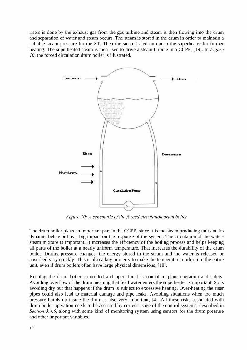
risers is done by the exhaust gas from the gas turbine and steam is then flowing into the drum and separation of water and steam occurs. The steam is stored in the drum in order to maintain a suitable steam pressure for the ST. Then the steam is led on out to the superheater for further heating. The superheated steam is then used to drive a steam turbine in a CCPP, [19]. In Figure 10, the forced circulation drum boiler is illustrated.

Figure 10: A schematic of the forced circulation drum boiler

The drum boiler plays an important part in the CCPP, since it is the steam producing unit and its dynamic behavior has a big impact on the response of the system. The circulation of the water-steam mixture is important. It increases the efficiency of the boiling process and helps keeping all parts of the boiler at a nearly uniform temperature. That increases the durability of the drum boiler. During pressure changes, the energy stored in the steam and the water is released or absorbed very quickly. This is also a key property to make the temperature uniform in the entire unit, even if drum boilers often have large physical dimensions, [18]. Keeping the drum boiler controlled and operational is crucial to plant operation and safety. Avoiding overflow of the drum meaning that feed water enters the superheater is important. So is avoiding dry out that happens if the drum is subject to excessive heating. Over-heating the riser pipes could also lead to material damage and pipe leaks. Avoiding situations when too much pressure builds up inside the drum is also very important, [4]. All these risks associated with drum boiler operation needs to be assessed by correct usage of the control systems, described in Section 3.4.6, along with some kind of monitoring system using sensors for the drum pressure and other important variables.

19

3.4.3 The Economizer The economizer is a heat exchanger that is used to pre-heat the feed water before it enters the steam producing part of the HRSG. It is located between the feed water pump and the drum boiler. It can consist of one or several steps, where each step is a separate heat exchanger. The feed water is heated up by using the lowest-temperature exhaust gas from the gas turbine. This is since the economizer is placed after the superheaters and the drum boiler, which are components that already extracted heat from the exhaust gas, [12]. The heating of the feed water should not be too large to avoid formation of steam bubbles in the economizer during abnormal conditions. This could lead to vibrations and water hammer, which is an unwanted pressure wave that can cause severe damage to the unit. By pre-heating the feed water using the economizer, the overall efficiency in the HRSG is increased with respect to the energy content of the exhaust gas. The economizer is constructed for heating of the feed water before entering the drum, by using the exhaust gas from the GT containing the least amount of energy, [17].

3.4.4 The Superheater The superheater is also a heat exchanger but it plays a different part than the economizer in the HRSG system. This component is used to heat up the steam exiting the drum boiler by using the highest-temperature exhaust gas from the gas turbine. The superheater can consist of several steps where each step is a separate heat exchanger. The purpose of the superheater in the CCPP is to raise the steam temperature from saturation conditions in order to make it superheated. Superheated steam decreases steam heat rate of the steam turbine, improving the turbine and overall plant power output and efficiency. It is important that the steam turbine is provided with steam that has the right properties so that it operates under the conditions that is was designed for. The purpose of using the superheater together with its controller, described in Section 3.4.6.3, is to ensure these proper operation conditions. If this fails and droplets would form that then enters the steam turbine, it can severely damage the turbine blades, [20]. The function of the superheater is to generate superheated steam by absorbing the heat by the metal tubes of the superheater, and consequently, by the steam inside the superheater. The properties of steam flow from the drum and exhaust gas exiting the gas turbine influences the dynamics of the steam in the superheater, [21].

3.4.5 Supplementary Firing Supplementary firing burners can be installed in order to increase the power of the CCPP. Supplementary firing also decreases the specific plant investment cost, [4]. The supplementary firing raises the temperature of the exhaust gas. There are different options when deciding the placement of the burners, but one solution is to place them between two of the superheater steps.

3.4.6 The HRSG Control System The different controllers in the HRSG are all crucial to ensure a safe and efficient operation of the power plant. There are many risks associated with the behavior of the HRSG that needs to be assessed. The control systems are based on usage of PID-controllers. They are the most commonly used controllers in industrial applications. If the reader is not familiar with the usage

20

and function of the controller there are many books and internet resources on the subject, such as [27]. One risk associated with the drum boiler process is the possibility that a poorly controlled drum boiler can result in damage to the steam turbine. The drum boiler is the source of steam for the turbine and if the steam is not heated sufficiently it might contain water drops. That leads to the possibility of the steam flow carrying water drops into the turbine and that damages the turbine blades severely, due to high rotation speed. An explanation of the function and purpose of each controller are given in Section 3.4.6.1-3.4.6.3 below.

3.4.6.1 The Inlet Valve Differential Pressure Controller In order to ensure that the feed water inlet valve can function properly, the pressure over this valve, called the differential pressure, can be controlled. The purpose is to give the inlet valve good operating conditions. This is done by measuring the pressure before and after the valve. Then the difference in pressure is calculated and sent to a PI-controller. This controller uses a set point in order to control the rotation speed of the feed water pump. The feed water pump then affects the pressure over the valve by pumping the right amount of feed water and in this way, the pressure over the drum boiler feed water inlet valve is controlled, [4].

3.4.6.2 The Drum Level Controller The purpose of the level control is to maintain the water level in the drum. That is an important issue in power plant control, since poor level control can result in a power plant trip (meaning that one or more components, or the whole plant, needs to shut down due to malfunction). The control of the drum level is problematic because of the dynamics of the water and steam mixture in the drum boiler. The redistribution of steam and water cause the so called shrink-and-swell effect. This is an important phenomenon to understand and describe in order to simulate the drum level behavior correctly. The shrink and swell refers to the behavior of water level in the drum and it occurs during fast load changes. If there is a sudden increase in steam demand, the pressure inside the drum drops. The pressure drop causes steam bubbles below the liquid level to swell, and that is why the level in the drum initially increases before it starts decreasing after a while. When the load suddenly drops, it leads to a pressure increase inside the boiler. Now the feed water flow is reduced and the bubbles shrink, so that the level in the drum decreases. The bubbles beneath the surface shrink and swell, and they change the volume of water and steam in the drum in response to pressure and heat variations. The total mass of the water-steam mixture in the entire drum boiler remains the same. This needs to be considered when the drum level controller is chosen and tuned, [18]. The drum boiler level controller can be of different types, depending on what input signals are measured and used in order to control the water level in the drum. Most drum boilers have level control which utilizes a three-element controller. This controller uses three different inputs to control the level. This control is achieved by balancing the feed water mass flow in to the drum against the steam mass flow out of the drum. Then, to minimize the drum level error a second

21

controller is used in a cascade arrangement. See Figure 11 for schematics of the three-element controller setup.

Figure 11: Schematics of the system for a three-element level controller of the drum boiler

When using the three-element controller and operating the power plant at low loads, instability can occur. This is due to the fact that the measurements of the small mass flows are unreliable. To avoid such problems, one has to switch to simple level feedback control, which is a single element controller that only uses level measurement, [22]. Another option is to use the two-element controller. This uses both measurements of the drum level and the feed water flow rate for the level control, see Figure 12.

Figure 12: Schematics of the system for a two-element level controller of the drum boiler

3.4.6.3 The Superheater Steam Temperature Controller In order to ensure that the steam leaving the HRSG from the superheater is in fact dry, i.e., superheated at the correct temperature, a temperature controller injects colder water, for example led from the feed water flowing into the economizer. One spraying device, or in some cases two, can be placed between two of the initial steps in the superheater. Exact positions depend on the

22

design of the superheater, e.g., how many steps it possesses. The controller makes sure that the right amount of spray water is injected so that it cools down the superheated steam just enough to keep its temperature at the correct level at the outlet of the last superheater step. Keeping the steam temperature stable, while transferring it to the steam turbine, is crucial for maintaining efficiency during operation and reduce fatigue and material stress in the steam turbine blades. This objective is difficult to achieve. One reason is that there is a time delay between the injection of spray water and when the steam temperature is measured, [24].

3.5 The Feed Water System The feed water system can have different designs depending on the type of plant where it is used. The system often includes a tank. The feed water tank serves as a large storage unit for the feed water. The purpose of the feed water system is providing the required amount of deaerated feed water to the HRSG. Deaeration is done in order to remove oxygen and other unwanted dissolved gases from the water. The flash steam from the blow down system in the plant is also led here. The function of the feedwater system is to supply high-pressure water to the boiler. The feedwater system also supplies water for the sprays that control the superheat steam temperature. When the feed water tank is used in a water-steam cycle the level in the feed water needs to be controlled. The level in the feed water tank is controlled using a PID-controller. The inputs to the controller are measurements of the water level in the tank using a level indicator and a pre-determined set point. The output of the controller can then be used to control the opening of a valve, or the rotation speed of the condensate pump, in order to regulate the mass flow rate into the tank. The tank functions as a buffer within the water-steam cycle in the CCPP. A typical feed water system always includes at least one or many feed water pumps. The purpose of the feed water pump is to supply the HRSG with feed water that can be used for the production of steam. The feed water pump is a powerful component that is large enough to pump liquid water from the condenser into the economizer. In a CCPP, the highest pressure point is after the feed water pump, since it must cover all the pressure losses in the HRSG and supply the ST with its operating pressure. Sometimes several pumps are connected and working together simultaneously in order to supply the HRSG with enough feed water. [25].

3.6 The Gas Turbine A gas turbine has several advantages as a power source. It can be easily assembled and erected and it can have an efficiency ranging from 25% to 40%. They also require less cooling water than other prime movers, [17]. They come in a wide variety of sizes and power outputs and have several applications. The main components in a gas turbine are the compressor, the combustion chamber, and the actual turbine coupled to a generator. The compressor drives air into a combustion chamber. In the combustion chamber the mixture of air and fuel is ignited. The combusted hot mixture makes the turbine work and it transforms the energy from the hot gas into kinetic energy. The kinetic energy is then used to drive the compressor and the generator for the production of electricity. A way to describe this process is by using the Brayton Cycle that was described earlier. The exhaust gas temperature is high, which helps to generate high-pressure and high-temperature superheated steam in the HRSG, [17].

23

Figure 13: A 3D illustration of the SGT-750. It is the machine most recently developed by SIT in

Finspång with a power output of 37 MW

3.7 The Steam Turbine In this section some background about the steam turbine is given. Then, only the inlet pressure controller is explained since the model only covers that part of the steam turbine control system.

3.7.1 General Description A steam turbine is a mechanical device that converts energy in steam into mechanical work. It can drive a generator to produce electricity. Industrial steam turbines are one of the most common prime movers in the world, and they are used for a variety of applications, [23]. The steam energy is converted to mechanical work by expansion through the stages of the turbine. The steam turbine employs a rotor, which is the rotating part and a stator, which is stationary. An impulse turbine use the velocity of the steam flow, and it changes the direction of the flow to create an impulse on the turbine blades, in order to make the turbine spin. There is very little pressure drop across the rotor [4]. In a steam turbine of reaction type the pressure drop occurs across both the rotor and the stator. The steam flow accelerates through the stator and decelerates through the rotor, and it does not result in any net change in steam velocity. The pressure drop corresponds to the work performed in the driving of the rotor, [12]. Another way of categorizing the steam turbines is to look at the exhaust pressures. The condensing turbines operate with exhaust pressures less than atmospheric pressure. The back-pressure turbines operate with exhaust pressures that are equal or greater than the atmospheric pressure. As a general rule, condensing turbines have a larger power output. Back-pressure turbines are smaller than a corresponding condenser turbine. Those turbines usually operate at much faster rotational speeds to increase efficiency, [23]. In a CCPP, a condensing steam turbine uses the superheated steam from the HRSG to produce electricity, and there are also possibilities to extract steam for other purposes through openings in the turbine casing between two of the stages.

24

Figure 14: The SST-600 steam turbine is constructed at a Siemens site in Germany

3.7.2 The Steam Turbine Inlet Pressure Controller A steam turbine has many controllers to govern the speed, load and turbine parameters to ensure that the turbine work under proper operating conditions. One of the turbine parameters that can be controlled is the pressure at the turbine inlet. The steam turbine controller is essentially a PID-controller that works to keep the inlet pressure at a certain reference point so that the steam parameters for the turbine at the inlet are correct during operation. The controller output governs the opening of the inlet valve to the steam turbine, [23]. Another way to operate the steam turbine is to use a control principle called sliding pressure. This means that the steam turbine inlet valves are fully open and the steam pressure is varying with the steam flow down to a certain minimum pressure level. In this case, the steam pressure at the HRSG outlet, minus the pressure losses in connecting piping, sets the pressure for the ST, [4].

3.8 The Condenser The condenser is a device used in steam turbines to condensate the steam that exit the steam turbine. The condenser is also a type of heat exchanger but with a different purpose than in the economizer or in the superheater. A common type in industrial application is the shell and tube heat exchanger, where the heat is removed from the steam by the use of a cooling medium, usually air or water. Surface condensers use the shell and tube heat exchangers. They consist of a large vessel containing a large number of tubes, some of them finned tubes, in order to enlarge the heat transfer area.

25

An air cooled condenser is chosen when cooling water is short of supply, but it is a more expensive solution than the water-cooled condenser, [14]. One way of increasing the overall efficiency of a CCPP is to maintain a low pressure in the condenser. The mass flow rate often needs to be considerably higher on the cooling side in order to make the steam condensate. The condensed steam is then pumped through to the feed water tank using a condensate pump.

Figure 15: A water cooled condenser that is to be installed on site

26

4 The Models The availability of steam at the correct thermal conditions and at the correct mass flow rates are key properties during the operation of any thermoelectric power plant, including CCPPs, [26]. Modelling the dynamic processes in the components of the CCPP is therefore an important challenge. In this chapter, the dynamic models that were developed and used in the work with this thesis are described. All models were developed using Dymola and its Modelica Standard library (MSL) along with the SiemensPower library. Focus lies on the models that were developed, but a description of the use and slight modifications of existing models are also included. It is necessary to include some information about them since they form a large part in the complete CCPP model presented in Section 4.6.

4.1 Simple Model of a Heat Exchanger The heat exchanger comes in many forms and shapes and they have different applications. When developing the HRSG model there was a need for simple co-current and counter current heat exchanger models with low simulation times. These would then be used for modelling of the economizer, for the risers and for all of the super heater steps.

4.1.1 Requirements and Limitations The requirements for the heat exchanger were that it should capture the essential properties of the heat exchanger while maintaining compatibility and low simulation times. Another important requirement was later identified to be the robustness of the model. Here it means that the model should have low sensitivity to the start-up values and pre-set parameters, so the number of simulation failures should be kept as small as possible when the model is a part of a larger one. The dynamics of the heat transfer and the influence of friction and other details are not captured by the model. The advantages are that the models are fast, easy to use, compatible and that they are valid at certain static operation points. The model is also flexible since the media can be switched, and also the direction of the passing media, making it easy to model both the co-current and the counter current heat exchangers. This model forms the basis of the economizer, the superheater steps and also the heat transfer calculations in the model of the risers.

4.1.2 Existing Model Investigation Models from two different libraries were tested, a standard heat exchanger model from the MSL library and a simple heat exchanger from the SiemensPower library. During tests it was concluded that the model from the MSL library did not meet the robustness requirement since it too often caused failed simulations when it was a part of a larger model. The SiemensPower library contained a simple heat exchanger that was easy to use and it also met the robustness requirement. Accuracy and simulation times depend strongly on a parameter that sets the number of segments that the pipe in which the water/steam medium flows is divided into. This division sets how the heat transfer calculation from the hotter gas medium to the water/steam medium is performed. This model has been proven to work well as a part of a complete CCPP model. A comparison in accuracy and simulation times was done in Section 5.1 to investigate differences between it and the developed model. There is a slight advantage when it comes to simulation times to the developed model and when it comes to accuracy, the

27

SiemensPower heat exchanger has varying accuracy that improves with the number of segments used in the heat transfer calculation.

4.1.3 Functional Description The simple heat exchanger is using the average temperature of its passing fluids to calculate the heat transfer. The schematic for the counter current heat exchanger model is found in Figure 16. The pressure losses that occur in the heat exchanger on both sides are modeled using linear valves. The pressure losses are larger on the water/steam side than on the gas side, so the valves are tuned differently. The geometries of the many pipes in the heat exchanger are simplified. They are represented with volumes with the contained mediums used in the heat exchanger. The volumes of the amount of the respective mediums are set with two parameters. The heat transfer is done using the equations presented in Section 4.1.5, and the amount of heat transfer is manually controlled by setting a heat transfer coefficient.

Figure 16: The counter current heat exchanger model used in the economizer model. Heat from the gas side is transferred to the water side

4.1.4 The Model Interface The drum boiler model is designed to be used as a part of a larger model for a complete HRSG in a CCPP. The interface is therefore made with standard Modelica Fluid connectors. The model uses medium functions from MSL on the water/steam side and medium functions from the SiemensPower library on the gas side.

28

4.1.5 The Simple Heat Exchanger Model Equations The amount of heat that is transferred depends on the mass flow rate and temperature of the passing media. The average temperature of the first medium, inside the risers is calculated using the following formula:

mT ,1

2,1,1

,1outin

m

TTT

+= (4.1)

where is the temperature at the inlet for the volume of medium 1 and is the temperature at the outlet. The average temperature of medium 2, denoted , is calculated in the same way:

inT ,1 outT ,1

mT ,2

2,2,2

,2outin

m

TTT

+= (4.2)

where is the temperature at the inlet for the volume of medium 2 and the temperature at the outlet. The amount of heat transferred, denoted Q , is then calculated with the following formula:

inT ,2 outT ,2

)( ,1,2 mm TTkQ −= (4.3)

where denotes the heat transfer coefficient. k

4.2 The Heat Recovery Steam Generator Model In this thesis a single pressure HRSG with a forced circulation drum-type boiler has been developed. The HRSG model consists of several sub components; the drum boiler model, the economizer, the superheaters, supplementary firing and three different controllers. The drum boiler level controller comes in three different versions, depending on the desired controlling method. The Superheater has four different steps. The diagram layer in Dymola for the developed HRSG is seen in Figure 17.

29

Figure 17: The model of the HRSG and its controllers. The surroundings of the model are described with the black text in the figure

Figure 17 only covers the top level of the model graphically. When clicking on each of the sub models, more detail appears. Sections 4.2.1-4.2.3 describe the sub models in the HRSG and Section 4.2.4 describes the controllers. The exhaust gas stack, which leads the gas out of the HRSG, is modeled with a valve and a sink. These models are found in the MSL and they are connected to the exhaust gas output from the economizer.

30

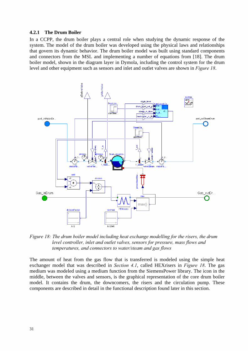
4.2.1 The Drum Boiler In a CCPP, the drum boiler plays a central role when studying the dynamic response of the system. The model of the drum boiler was developed using the physical laws and relationships that govern its dynamic behavior. The drum boiler model was built using standard components and connectors from the MSL and implementing a number of equations from [18]. The drum boiler model, shown in the diagram layer in Dymola, including the control system for the drum level and other equipment such as sensors and inlet and outlet valves are shown in Figure 18.

Figure 18: The drum boiler model including heat exchange modelling for the risers, the drum level controller, inlet and outlet valves, sensors for pressure, mass flows and temperatures, and connectors to water/steam and gas flows The amount of heat from the gas flow that is transferred is modeled using the simple heat exchanger model that was described in Section 4.1, called HEXrisers in Figure 18. The gas medium was modeled using a medium function from the SiemensPower library. The icon in the middle, between the valves and sensors, is the graphical representation of the core drum boiler model. It contains the drum, the downcomers, the risers and the circulation pump. These components are described in detail in the functional description found later in this section.

31

4.2.1.1 Requirements and Limitations The requirements of the drum boiler model are presented in Table 1 below. Requirement Motivation 1 The model should be efficient so the CPU

load during simulation is minimized.

So that the model can be used as a part of a CCPP model that meets the efficiency demands on a PC with normal performance.

2 The model should capture the dynamics related to drum water level and pressure control.

Studying the performance of different control strategies and the performance of the controllers is important.

3 The model should be based mainly upon geometrical and physical parameters.

Having too many empirical parameters that need to be tuned decreases the applicability of the model.

4 The model should capture important dynamic characteristics over a wide operating range.

Studying drum boiler behavior at different loads, and be able to trust those results, is important. Then it becomes possible to perform analysis of the component during disturbances such as plant trips.

Table 1: Requirements along with their motivations for the drum boiler model

There are a number of limitations in the developed model. The limitations are presented in Table 2 below. Limitation Comment 1 Two-phase flows are generally

complicated phenomena, and the model does not capture the detailed behavior. The steam and the water in the drum boiler flow at different rates and there is slip between them because of the density difference between the two phases (the water phase and the steam phase).

This is a limitation which is claimed to be of small importance according to reference [18] pp. 367.

2 The drum boiler model behavior is not to be investigated during start-up and shut-down in the scope of this thesis.

This model is suitable for simulation of a HRSG in operation, subjected to different disturbances. It is not tested during start-up and shut-down.

3 The blow down valve used for depressurizing in case of emergency is not included in the model.

-

Table 2: Limitations along with comments for the drum boiler model

32

4.2.1.2 Existing Model Investigation Before the development of the drum boiler model commenced, other models were studied to investigate if they were useful as starting points or as references. The MSL contains a drum boiler model. The model is simple and it lacks models of the downcomer and riser tubes. Neither the drum level is modeled in detail, nor is the geometry of the drum. Thus, the model does not meet the specified demands, but it did serve as a good starting point for the design. A few other models were also found and investigated in other libraries, such as the SiemensPower library, but two of the models found in other libraries were incompatible with the Modelica Fluid Library since they used other types of connections. The SiemensPower model was compatible, but there, as in the other models, the main problem was a lack of documentation and specification of sources for the equations used. The decision was made to implement a theoretical model. This was done using a number of equations described in a frequently cited scientific article, Drum-boiler dynamics by Åström and Bell as a starting point in the development process. The theoretical model in that article was assessed to have the potential to be implemented and modified in order to meet the requirements posed on a drum boiler model.

4.2.1.3 Functional Description A drum boiler is large and has a complicated geometry, because of its many downcomer and riser tubes. In spite of this, studies have shown that the gross behavior of the system can be captured by usage of simple global mass and energy balances. When the pressure changes in the boiler the energy stored in the steam and water is released or absorbed rapidly. All different parts of the drum boiler change their temperature in the same way. This property of the drum boiler makes it possible to use a model of low order to capture the essential dynamics, [18]. The developed drum boiler model makes use of this theory, since the global energy and mass balances are implemented. In Figure 19 the icon layer view of the core drum boiler model is shown. This core model uses MSL connectors for the inputs and the outputs. The core includes the equations describing the dynamics of the drum boiler system. The code was written using the ability in Dymola to use different levels when modelling. This was done so that the equations for the different parts is implemented using the same logical structure as the structure of the parts in the physical component.

33

Figure 19: The drum boiler model shown in the icon layer. Connectors to the economizer, the

superheater, heat to the risers and drum level measurement are marked in the figure See Figure 20 for schematics of the component at a lower level. This level of detail is reached graphically in Dymola by simple navigation in the modelling view of the program. This schematic serves as a flow diagram for the activities and dynamic behavior that the model development takes into account.

Figure 20: The diagram layer of the drum boiler components in Dymola. The components are

the drum, the downcomers, the risers and the circulation pump

34

The functions of the models of each of the components in the drum boilers are described in Section 4.2.1.3.1-4.2.1.3.4 below. 4.2.1.3.1 The Drum The drum geometry is modeled. It is assumed to be cylindrical and there is an option to make it either horizontally or vertically oriented. The medium model used inside the drum has a two-phase property so that it can represent both steam and water. The water level in the drum is then controlled by the control system that was modeled separately, and it is described in Section 4.2.4.2. 4.2.1.3.2 The Downcomers The water is flowing down the downcomers and the friction losses are accounted for. The model has parameters for the geometry, the number of tubes and the surface roughness since it uses a pipe model from MSL. 4.2.1.3.3 The Risers In the drum boiler risers, the water is heated up from an external heat source until it starts to boil and steam bubbles rise to the drum. The model for the risers consists of two parts. One part is the piping that uses a pipe model from MSL. The other part describes the heat supplied to the risers. This part is modeled using Equation 4.11 and Equation 4.12 which are found in Section 4.2.1.6. The distribution of steam in the risers is modeled using equations from [18]. The two parts of the model of the risers and model connections are seen in Figure 21.

Figure 21: The schematics of the model of the risers

Modelling the amount of heat supplied is done using the simple heat exchanger model described in Section 4.1. The amount of heat available and needed to make the water boil inside the risers depends on the mass flow rate and temperature of the passing exhaust gas, but also the pressure, the starting temperature and the mass flow rate of the water flowing in from the economizer. The average temperature of the water-steam mixture, denoted , inside the risers is calculated using the following formula:

mwrT ,

35

2,,

,outwrinwr

mwr

TTT

+= (4.4)

where is the temperature at the risers inlet and the temperature at the risers outlet. The average temperature of the exhaust gas, , is calculated in the same way:

inwrT , outwrT ,

mgrT ,

2,,

,outgringr

mgr

TTT

+= (4.5)

where is the temperature at the risers inlet and is the temperature at the risers outlet. The amount of heat, denoted Q , is then approximated using the following formula:

ingrT , outgrT ,

)( ,, mwrmgr TTkQ −= (4.6)

where denotes the heat transfer coefficient that governs the amount of heat that is supplied to the two-phase medium inside the riser pipes.

k

4.2.1.3.4 The Circulation Pump A MSL pump model was used for the circulation pump. The flow characteristics of the circulation pump describe the relationship between the pump head [m] and volume flow rate [m3/s]. The circulation pump has quadratic flow characteristics. The relationship is defined by choosing three different operating points for the pump. Then the range of operation is obtained, and in order to function properly, the pump has to operate within these sets of parameter ranges. Other parameters that needed to be set were for example the nominal values for mass flow rate and pressures at the pump inlet and outlet.

4.2.1.4 Variables and Parameters In the drum boiler core model, a number of parameters and variables are used to describe the physics and dynamics of the drum boiler. The variables are listed alphabetically in Table 1 in Appendix A, as well as explained where they first appear in the equations. Since the downcomers and the circulation pump are standard Modelica models, which are only subject to changes in the parameters, there is no need to list those variables. The drum boiler core model parameters are listed in Table 2. Here the parameters of the downcomers and the pump are included.

4.2.1.5 The Model Interface The drum boiler model is designed to be used as a part of a larger model for a complete HRSG in a CCPP. The interface is therefore made with standard Modelica Fluid connectors. The model also uses the medium functions from the MSL. In order to model the drum boiler correctly, appropriate inputs and outputs to and from the component needs to be defined. The model should be directly connected to the superheaters and to the economizer in order to form the HRSG model together. The heat from the exhaust gas from the gas turbine should evaporate the feed water in the riser tubes to produce the steam flow out to the superheaters.

36

The input heat from the hot exhaust gas is denoted Q. Feed water flows into the drum and the steam flow that rises above the water level surface is separated and led out of the drum to the superheaters. 4.2.1.5.1 Input The first model input is the feed water that comes from the economizers. The feed water is described by its mass flow, denoted qf, its pressure pin and the specific enthalpy of the feed water, hf. The feed water is pumped through the economizers to the drum from a feed water tank. The last input is the heat flow Q from the exhaust gas that is calculated using the medium temperatures at the risers inlet and outlet. 4.2.1.5.2 Output The first model output the steam that flows out through the superheater and then on to the steam turbine. The steam out of the drum is described by its mass flow rate qs, its pressure, pout and the specific enthalpy of the steam, hs. Finally, the drum level output is denoted . drumlvlL ,

4.2.1.6 The Drum Boiler Core Model Equations In this section, the equations that describe the dynamic behavior of the drum boiler are reported and explained. The total volume of water/steam in the drum boiler, (including the downcomers and risers) is: tV

wtstt VVV += (4.7)

where - Total volume of steam in the drum boiler. stV

wtV - Total volume of water in the drum boiler. The global mass balance in the system is:

wtwstst VVM ρρ +=

sft qqMdtd

− = )( (4.8)

where - Total mass of water/steam in the drum boiler. tM

sρ - Density of steam. wρ - Density of water. - Mass flow rate feed water. fq - Mass flow rate steam. sq If denotes specific internal energy, the total energy contained of the system, denoted , of the system is:

u tE

mpmtwtwwstsst tCmVuVuE ++ = ρρ

37

where - Internal energy steam. su - Internal energy water. wu

mtm - Total mass of metal drum boiler.

pC - Specific heat capacity of drum boiler metal material.

mt - Temperature of drum boiler metal.

The factor represents the contained energy in the metal walls of the drum boiler. mpmt tCm The internal energy is described by the following expression:

ρphu − =

where - Specific enthalpy. h - Pressure. p

ρ - Density.

If the expression for above is used to reformulate u stss Vuρ and wtww Vuρ we get:

=⎟⎟⎠

⎞⎜⎜⎝

⎛−= VphVu

ρρρ pVVh −ρ

where - Volume. V That means, when inserting Equation 4.7 and using the relationship above, the internal drum boiler energy of the system, , can be reformulated in the following way: tE

mpmttwtwwstsst tCmpVVhVhE +−+ = ρρ (4.9)

where - Specific enthalpy of steam. sh - Specific enthalpy of water. wh

p - Pressure inside drum boiler.

Equation 4.9 holds when assuming total thermal isolation of the drum boiler wall. The change in drum boiler energy is given by the power balance:

ssfft hqhqQEdtd

−+ =)( (4.10)

where - Heat flow rate to the risers Q

fh - Specific enthalpy feed water

38

Hence the differentiation of Equation 4.9 must fulfill the power balance described by Equation 4.10. These equations states how the internal power of the system can be calculated. Here it is assumed that no heat losses to the surroundings are present. Equations 4.7-4.10 captures the overall behavior of the boiler quite well, but it does not capture the different phenomena that are related to the distribution of water and steam in the drum boiler. And those phenomena are necessary to capture in order to model the drum level, [18]. Therefore, Equation 4.11 - 4.17 are introduced to take into account the riser tubes and the different flows within the drum boiler. Mass and energy balances of a heated tube section are used to find a function describing the distribution of steam in the risers when it is heated up, see [18, p. 367] for the derivation. The mass steam fraction along the riser, denoted mα , is expressed as: ξαα rm = where rα - Steam quality at the risers outlet, 10 ≤≤ rα . ξ - Normalized length coordinate along the risers, 10 ≤≤ ξ . The volume fraction of steam, denoted rvα , and mα have the following relationship for a saturated water/steam mixture:

msws

mw

αρρραρα

)(rv −+=

The average volume fraction, denoted rvα , is of interest since it governs the total amount of steam in the risers. It can be calculated in the following way:

...)(

)(1

0

1

0rvrv =

−+== ∫∫ ξ

ξαρρρξαρ

ξξαα ddrsws

rw

Intermediate steps in solving of the integral above have been omitted. The solution is that the average volume fraction of steam in the risers is:

⎟⎟⎠

⎞⎜⎜⎝

⎛⎟⎟⎠

⎞⎜⎜⎝

⎛ −+

−−

−= r

s

sw

rsw

s

sw

w αρ

ρραρρ

ρρρ

ρα 1ln)(

1rv (4.11)

Equation 4.12 - 4.14 below describe the balance of mass and energy in the risers. The same reasoning as for the previous balances, presented in Equation 4.8 - 4.10, is used here, but only for the risers. Mass balance for risers:

rwrs VVM )1( rvrvr αραρ −+=

rdcr qqMdtd

−=)( (4.12)

39

where - Total mass risers. rM

dcq - Mass flow rate in downcomers.

rq - Mass flow rate in risers.

rV - Volume risers. Energy balance for risers:

( ) spmrrrwwrssr tCmpVVhVhE +−−+= rvrv 1 αραρ (4.13)

rwwsrwdcr qhhhhqQEdtd ))(()( +−−+ = α (4.14)

where - Total energy risers. rE

mrm - Mass of metal risers. - Temperature saturated steam. st The distribution of steam in the drum is captured by Equation 4.15, 4.16 and 4.17. Mass balance for steam under the drum water level gives the following equation:

sdsVM ρ= sd

sdcdrrsd qqqMdtd

−− = α)( (4.15)

where - Mass of steam bubbles drum. sdM - Volume of steam in drum under the liquid level. sdV - Condensation mass flow rate drum. cdq

sdq - Steam flow rate through the liquid surface in drum. The condensation flow rate in the drum, denoted , is expressed using the following equation: cdq

⎟⎠⎞

⎜⎝⎛ ++−+

−+

−−

=dtdtCm

dtdpVV

dtdhV

dtdhV

hhq

hhhh

q spdwdsd

wwdw

ssds

wsf

ws

fwcd )(1 ρρ

(4.16) where - Volume of water in drum. wdV The first term in Equation 4.16 above is the condensation due to heating the incoming feed water flow. The second term is the condensation due to the change of internal energy of the drum, where derivatives of densities and volumes are negligible compared to the terms containing derivate of the enthalpy. The derivatives of densities and volumes have less than 1% influence of the other terms in the whole operating area, so they are neglected here. The energy impact of downcomers, risers and steam leaving drums water volume are accounted for by the change in internal energy of the drum water, and this is reflected by the second term.

40

For a derivation of Equation 4.16, see [18, p. 368]. The steam flow through the liquid surface in the drum is captured using the following equation:

)()( 0rdcrdcrsdsd

d

ssd qqqVV

Tq −++−= βαα

ρ (4.17)

This equation includes the parameters β, Td and that are all empirical. The default values used is β = 0.3 and T

0sdV

d = 5 s, that denotes the residence time for steam in the drum. denotes the hypothetical situation when there is no condensation of steam in the drum. The default value of this parameter is set to = 12m

0sdV

0sdV 3. These parameters were taken from the drum boiler

verified in [18], or set using certain assumptions from simulation experiments. Since the drum boiler is verified against data from KRAWAL they are seen as sufficiently good assumptions. But, if high accuracy in the simulation is needed, data measurements on the drum boiler that are to be simulated should be used in order to better tune these parameters. If all the water volumes in the drum boiler are added up, we get the following equation: riserswdcwdwt VVVV ,++= where - Volume of water in downcomers dcV - Volume of water in risers riserswV ,

Thus, the volume of water in the drum can be expressed using the following equation:

rrvdcwtwd VVVV )1( α−−−= (4.18)

The drum level is calculated using this equation, since the distribution of steam below the drum level is now accounted for:

d

sdwddrumlvl A

VVL

+=, (4.19)

where is a parameter for the liquid surface at the normal operating level. In the most common case, this operating level is in the middle of the drum.

dA

With all these equations, the dynamics of the drum boiler is described. In order to extract more information from the system, some additional variables are also introduced so that they can be observed when simulating the model. Three additional variables for drum masses are introduced and calculated using these equations:

wddrumw VM w, ρ=

sddrums VM s, ρ=

drumsdrumwdrum MMM ,, +=

41

Four additional variables for masses and volumes in the risers are calculated using these equations:

riserswrisersw VM ,w, ρ=

riserssriserss VM ,s, ρ=

rrvrisersw VV )1(, α−=

rrvriserss VV α=,

4.2.1.7 Documentation Documenting the characteristics and properties of the drum boiler model has been an important part of the model development. In Dymola there is a documentation layer that can be edited for each model. This has been done for every component included in the model, see Figure 22.

Figure 22: The documentation view of the drum boiler model

Information about the model, its connectors and references etc. has been added to the documentation layer. The documentation of each of the models in this thesis also serves as model documentation. The Dymola text layer is where the code is edited. An effort to write structured code with extensive comments has been done. See Figure 23 for an example.

42

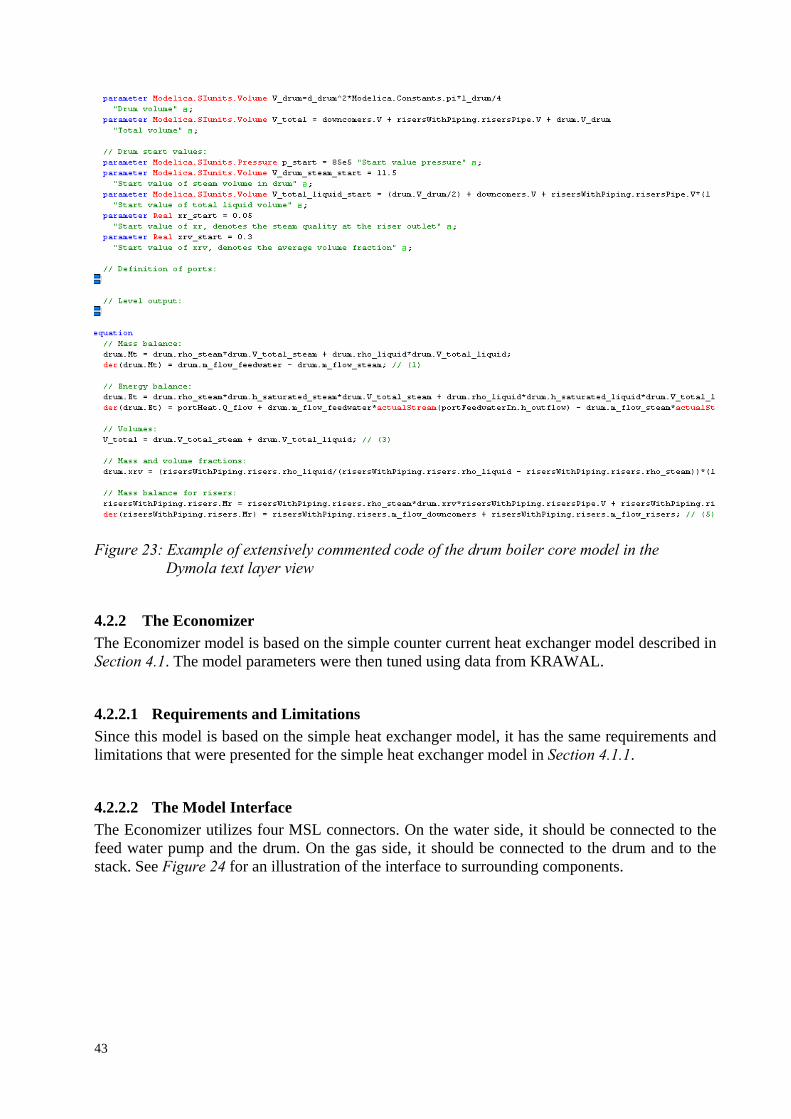
Figure 23: Example of extensively commented code of the drum boiler core model in the

Dymola text layer view

4.2.2 The Economizer The Economizer model is based on the simple counter current heat exchanger model described in Section 4.1. The model parameters were then tuned using data from KRAWAL.

4.2.2.1 Requirements and Limitations Since this model is based on the simple heat exchanger model, it has the same requirements and limitations that were presented for the simple heat exchanger model in Section 4.1.1.

4.2.2.2 The Model Interface The Economizer utilizes four MSL connectors. On the water side, it should be connected to the feed water pump and the drum. On the gas side, it should be connected to the drum and to the stack. See Figure 24 for an illustration of the interface to surrounding components.

43

Figure 24: The economizer model along with the feed water pump with explanations for the

connectors

4.2.2.3 Functional Description The Economizer model enables heat transfer between the hot exhaust gas that originally flows from the GT exhaust and the feed water from the feed water pump. The mediums are water and exhaust gas and the mediums flow in the opposite direction, therefore it is a counter current heat exchanger.

4.2.3 The Superheater The superheater model is built using four different steps. Each step is a simple heat exchanger, each one the same as the simple heat exchanger described in Section 4.1. So each step transfers a different amount of heat from the gas side to the water/steam side. The steps are connected to each other, but also to the supplementary firing model and the spray temperature controller. The mediums are steam and exhaust gas and the mediums flow in the same direction, therefore it is a co-current heat exchanger. The superheater parameters for each of the four steps were then tuned using data from KRAWAL.

4.2.3.1 Requirements and Limitations Since it is based on four connected simple heat exchangers, it has the same requirements and limitations that were described in Section 4.1.1. Additionally there is a limitation in the modelling of the spray water injection. It is assumed to be done by ideally mixing the colder spray water with the hot steam.

4.2.3.2 The Model Interface The superheaters utilize many MSL connectors to connect to each other and to supplementary firing, and they also have an inlet for spray water. On the steam side, the inlet to step 1 should be connected to the drum. The outlet of step 4 should be connected to the piping that leads to the steam turbine. On the gas side, there are connections to the GT exhaust, to the supplementary firing and to the gas side in the drum boiler. See Figure 25 for an explanation for the connectors and the superheater interface with its surroundings.

44

Figure 25: The superheater model with explanations for the connectors written in black text

4.2.3.3 Functional Description The superheater model enables heat transfer between the hot exhaust gas from the GT exhaust and the steam that was produced by the drum boiler and then led through the superheater. The amount of heat that is transferred in each of the modeled superheater steps differs. The amout is dependent on the dimensions and position of each of them. The steps vary in size and the prerequisites for the heat transfer changes for each of them since they have different positions relative to the GT exhaust gas outlet. The superheater step 4 is subject to a higher temperature in the exhaust gas than the superheater step 3. Superheater step 2 can be subject to high temperature since it is located next to the supplementary firing burners. Injection of spray water between two stages in the superheater is a method to achieve the desired final steam temperature out of the superheater. The amount of spray water that is injected is controlled by the spray temperature controller described in Section 4.2.4.3. The spray water

45

injection is done between superheater step 2 and superheater step 3. The spray water is taken from the feed water pump, so when injected it cools down the superheated steam. 4.2.3.3.1 Supplementary Firing The supplementary firing can be placed at different locations in the HRSG. Here, the supplementary firing is done in the superheater between the first two steps after the drum boiler, superheater step 1 and step 2.

Figure 26: The supplementary firing model. The connections to the superheater steps are

marked with black text There is a limitation in the maximum amount of heat that can be transferred from the burner to the superheater. This limitation is set because of the risk of damaging the material in the superheater pipes. There are also limitations in the temperature gradients to not risk causing material stress in the superheater. These limitations are not considered when modelling the supplementary firing, but they could be introduced in a simple way, since a table function is used to manually control the amount of heat flow to the passing gas, by supplying table data. The ideal heat source is used to transfer the heat to the passing gas. This model does not capture changes in the composition of the gas. In the real burning process the composition changes, and the amount of for example oxygen in the gas declines.

4.2.4 The HRSG Control System The HRSG control system is modeled using several PI-controllers, each of them serving a specific controlling purpose. The main controllers in the HRSG have been modeled. This includes the drum pressure and level controllers and the superheater steam temperature controller.

46

The basic component for all the controllers is the MSL component limPID which is a PID controller with the possibility to limit the output value from the controller.

4.2.4.1 The Inlet Valve Differential Pressure Controller The drum inlet valve differential pressure controller is modeled using pressure sensors to measure the pressure before and after the feed water inlet valve. Then a PI-controller is used to keep the pressure over the valve at a constant level, and that level is set by using a set point signal that is fed to the controller. This pressure over the valve is called the differential pressure. The PI-controller then regulates the speed of the feed water pump in order to control the differential pressure. If the speed of the pump increases, then the pressure rises over the feed water valve, and the opposite occurs if the speed decreases. See Figure 27 for the schematic of the controller.

Figure 27: The drum pressure controller controlling the differential pressure over the feed water

inlet valve by adjusting the speed of the feed water pump

4.2.4.2 The Drum Level Controller Models of three different approaches to the drum level control were developed. The three-element drum level controller is the most common, so therefore it is that controller model that is used for controlling the drum level in the drum boiler model by default. But it is possible to switch to one- or two-element controllers when needed. The differences between these controllers were explained in Section 3.4.6.2. The three-element drum level controller model is illustrated in Figure 28.

47

Figure 28: This illustrates where the drum level controller is situated and how it controls the

level of the drum using the feed water inlet valve to the drum

Figure 29 below explains how there are two controllers in cascade that together control the level. The difference in drum level measurement and drum level set point is driven towards zero using a P-controller. Then the mass flow rates in and out of the drum are balanced using the PI-controller.

48

Figure 29: The schematics for the three-element drum level controller. A cascade connection

between a P-controller and a PI-controller is utilized for the level control

4.2.4.2.1 Requirements and Limitations There is a requirement to keep the water level within the limits for the highest and lowest allowable water level in the drum. This is to prevent flooding and avoid the risk of damaging the evaporation tubes in the risers. The shrink and swell phenomenon that was explained in Section 3.4.6.2 makes variations in the drum level common. When subject to large disturbances, poor control of the water level may cause the level to fall below or exceed the allowable levels. That can result in expensive plant trips, serious damage to the drum, or carrying water over into the steam turbine, which will damage it. This leads to high demands on the performance of the control system. The water level is approximately in the middle of the drum and should be kept there to minimize the risk of flooding.

4.2.4.3 The Superheater Steam Temperature Controller The properties of the superheated steam exiting the last superheater step must be in a certain region to ensure the operation of the steam turbine. When utilizing a steam temperature controller, in the form of a controlled spray injection between two of the superheater steps, these desired properties can be obtained. A multi-step superheater often uses two spray injectors in order to control the temperature of the steam at the superheater outlet. In this model, only one spray is used. Additionally, the control system is often more sophisticated, controlling temperature, mass flow rate and also enthalpy in order to ensure stable operation of the superheater. Only the temperature part is included in this model, so the model of the controller is simplified.

49

The superheater steam controller is a PI-controller that has one measurement input which is the temperature after super heater step 4, which is the last one before the piping to the steam turbine. The controller then regulates the opening of a valve by using a temperature set point signal. This valve controls the amount of spray water that is taken from the feed water pump. There is a rule of thumb that one can inject no more than 10% (or in some cases, the limit is maximum 15%) of the mass flow in the feed water system as spray water [4]. If more than that is injected into the steam flow in the superheater the steam turbine might be subject to water drops and be severely damaged. The model is based on a limPID, so the output of the controller is limited so that the mass flow rate does not exceed this limit. See Figure 30 below for an illustration of this limit.

Figure 30: The top curves represent the spray water mass flow (blue) compared to 10 % of the

feed water mass flow after the pump (red). The bottom curves represent the temperature at the superheater outlet (blue) compared to the temperature set point (red)

In Figure 30 the CCPP is in steady state operation and the temperature is controlled. When the temperature set point is changed to a lower temperature, the amount of spray water must increase in order to reach the new temperature set point. This is not achieved in this case since the limit in the amount of spraying water is reached, and as a result the temperature out to the steam turbine piping is higher than the set point temperature. This is something that needs to be avoided in practice. In the design phase, the HRSG must be dimensioned so that all load cases where the CCPP is designed to handle has a functioning steam temperature control in the superheater, which does not inject too much spray water, while at the same time regulating the steam temperature sufficiently well.

4.3 The Feed Water System The feed water system is an important part of the CCPP since it enables continuous re-usage of the condensate water by the HRSG through storing it in a feed water tank and then pumping it on to the economizer. In Figure 31 the schematics for the feed water system is shown.

50

Figure 31: Schematics for the feed water system. The model surroundings and the different

components of the system are explained with the black text

4.3.1 Requirements and Limitations The requirements for the feed water system model are that the pumps are operational in a large number of operation points so that a complete CCPP model can be tested during larger disturbances. The feed water tank model should represent a buffer between the condenser and the HRSG, and it should also represent the storage of feed water. The level in the feedwater tank is controlled. The geometry of the tank is not modeled so the tank model is just a rough approximation of the real component. The level is controlled by regulating the mass of water in the tank. There is no drainage from the steam turbine included in the model. This drainage is normally led to the feed water tank to heat up the feed water. This is instead modeled using an ideal heat flow source. Another limitation is that the blow down system from the drum is not included in the scope of the modelling, so there are no pipes or valves representing this system in the feed water system model.

4.3.2 Functional Description The condensed water is pumped on to the feed water tank by the condenser pump. This condenser pump is controlling the level in the feed water tank by controlling the mass of water in the tank using a PI-controller. The feed water tank valve is fully open and is situated at the feed water tank inlet. This valve represents the pressure losses in the piping between the condenser pump and the feed water tank. After passing the inlet valve, the water is subject to heating using a prescribed heat flow in the large feed water tank. The feed water is after the storage in the tank pumped on through to the economizer using the feed water pump. This feed water pump also supplies water for the spray unit used in the superheater temperature control system. The condenser pump is situated after the condenser, and it is of the same type as the circulation pump described in Section 4.2.1.3.4, but with different dimensions and a different kind of characteristics. The condensate pump has linear characteristic, which means that the relationship

51

between the pump head [m] and volume flow rate [m3/s] is linear. The circulation pump and the feed water pump both have quadratic characteristics. All these pumps were modeled using standard models from MSL. The characteristics are chosen and adapted with respect to what the nominal mass flows and the nominal rotation speeds are. This also depends on the pressure at the pump inlet and outlet for each of the pumps. The characteristics were chosen to make the pump function well in a large area of operation.

4.3.3 The Model Interface The model uses MSL connectors and it is connected to the model condenser and to the economizer model. The speed of the feed water pump is controlled by the drum pressure controller that utilizes pressure sensors in the drum, sensors that are situated before and after the feed water inlet valve.

4.4 The Steam Turbine Inlet Pressure Controller Model The steam turbine inlet pressure is modeled using the MSL model limPID. Only the proportional and the integral part are used for the control. In the CCPP model, the steam turbine is running using a constant inlet pressure. There are other ways of operating the steam turbine, for example using a sliding pressure. In this mode the pressure set point follows a curve that keeps the valve nearly fully open, to improve efficency by reduced pressure losses over the valve. This is something that can be approximately employed in the model, by sending a constant signal to the valve that represents a 100 % opening. The PI-controller for the inlet pressure uses a measurement input from the pressure sensor and a set point to control the inlet valve so that the inlet pressure remains constant when the HRSG produces different steam flow rates. See Figure 32 for schematics for the pressure control.

Figure 32: The pressure controller model and the steam turbine inlet valve model are situated

adjacent to the steam turbine model

4.5 Adaptations of Other Models In order to complete the water-steam cycle in the CCPP model described in Section 4.6, a steam turbine model, a condenser model and a gas turbine model were needed. The SiemensPower library contained a well functioning model for the steam turbine and a slowly simulated but detailed model for the gas turbine. Regarding the condenser model, development of a model at Siemens was in progress so throughout the work with the thesis, several different models were tested. Finally a newly developed air-cooled condenser model was used in the CCPP model.

52

4.5.1 The Gas Turbine A Siemens SGT800 Gas Turbine (GT) model had already been developed at Siemens. Some minor modifications were made to it. Sensors for measuring mass flow rate and temperature were placed at the exhaust from the gas turbine model. The measurements were inputs to the exhaust gas source. The exhaust gas source from the gas turbine was then used as input for the HRSG-model. In order to be able to change the gas turbine load, the input for this was modified in the model. The input parameter was changed from a constant value to a ramp function in order to add the possibility to introduce sudden load changes. When developing the CCPP model there was a need to approximate the GT model since it makes the simulation run slowly. An approximation of the temperature and mass flow rate start up curves was done using a table function, obtaining many linear segments between different times, and filter the resulting signal through a standard linear filter to increase the curve’s smoothness. Start up curves for some different GT loads were modeled. Comparisons between the respective curves were made and the correlations are regarded as acceptable for the application.

4.5.2 The Steam Turbine A Steam Turbine (ST) model from the SiemensPower library was adapted to the operating conditions for the CCPP at certain gas turbine loads by using data from KRAWAL. The model is of a condensing, multi-stage, impulse turbine. In the model, the performance of each of the stages in the turbine is calculated according to Stodola’s law, [28]. The steam turbine model parameters were adapted so that the model would work under certain operating conditions. Nominal values for the pressure, the enthalpy and the mass flow were set to obtain realistic isentropic efficiencies for each stage of the ST model. The piping between the superheater and the steam turbine is represented by a volume and a valve, where the valve represents the pressure losses in the piping.

4.5.3 The Condenser The built CCPP model uses an Air-Cooled Condenser (ACC) model that is simple and fast but lacks a modelling of the condenser dynamics. Almost no adaptations were made to this model. The nominal mass flow parameter was set to the steam turbine model outlet mass flow rate. The default values were used for the other input parameters, such as the hotwell level. The CCPP model has also been simulated with a Water-Cooled Condenser (WCC) model. Changes of a few parameter values were made in order to size the condenser model in relation to the steam turbine model.

4.6 The Combined Cycle Power Plant Model The CCPP model contains all the different components described in Section 4.2–4.5. The components and their control systems have all been tuned to be integrated and well functioning together. Data from KRAWAL has been used for this tuning. The model forms a common form of a combined cycle; here a Brayton Cycle and a Rankine Cycle are combined. The schematic for the model is shown in Figure 33.

53

Figure 33: The complete CCPP model as seen in the Dymola diagram layer. The black text in

the red bubbles marks out the different main components that constitute the model.

In Figure 34 the different controllers are shown. As seen, there are five control systems that all need to operate simultaneously in order to reach a steady state operation of the CCPP. This required that the respective controllers were tuned so that they would not interfere with each other; they should operate in separate time scales. For example, the pressure controller could be fast with a higher gain, but the superheater temperature controller was tuned with a lower gain, being slower than the pressure controller. Poorly tuned control systems can cause chattering, which is a problem in the solver occurring during simulation. It is a phenomenon that slows down the simulation since the solver gets stuck switching between two events when trying to solve the system of equations. The system can also become unsolvable if each of the control systems are not adapted to the prerequisites in their surroundings.

54

Figure 34: The complete model as seen in the Dymola diagram layer. The black text in the red bubbles marks the position of the different controllers included in the model

4.6.1 Requirements and Limitations The requirements for this model were that it had to form a complete combined cycle in order to perform dynamic studies on a complete system. It had to include the most important components and the essential control systems, but it also had to be simple. This was so that the CPU load could be minimized so that a PC with normal performance is able to simulate the model within a time frame of 5 minutes for a typical test case. This test case is presented in Section 5.2. To keep the simulation time under 5 minutes posed requirements on the developed sub models that they would simulate much faster than that. If the time frame was kept, the simulation time was considered to be acceptable and the model was efficient enough to be useful when performing simulations. A requirement was posed on the model that it needed to be able to simulate a ramp from 100 % down to 25% GT load and then back up again to 100% load. This was to show that the model would not fail to complete a simulation of a disturbance of this magnitude. The limitations of the sub models described earlier are also transferred to limit the performance and accuracy of this complete CCPP model. Some notable limitations and simplifications in the components are:

• The boiler blow down system is not modeled. • Bypass operation is not possible in the model. This means that there is no possibility to

bypass the ST and lead steam or water to a drain or directly to the condenser without passing the ST.

• The geometry of the heat exchanger pipes is represented by volumes. • The supplementary firing modelling is simplified and does not affect the composition of

the passing gas. • There is no steam extraction from the steam turbine to heat the feed water tank. • The start-up and shut down of the CCPP can not be simulated.

4.6.2 Functional Description This model represents a CCPP, so on the water/steam-side, the Rankine Cycle, described in Section 3.1.2, is modeled. When the GT model is used, the whole Combined Cycle, explained in Section 3.3, is complete. Disturbances can be introduced in for example the GT-load, and then the system response of the complete CCPP can be studied in a simulation. Changes in controller set-up and other dynamic studies, such as for example studying effects of using different amounts of supplementary firing, can also be performed using this model.

55

5 Testing and Verification During the development of the models and the control system, they were subject to continuous testing in order to check their compatibility, how the models interact and if the dynamic and static behavior was as expected. A number of test results and different methods of verification used are reported in this chapter. The chapter starts with verification of the HRSG model. Then a smaller test case is described for the complete CCPP model in Section 5.2.

5.1 Verification of the HRSG Model The model for the HRSG is verified using a number of methods. Firstly, the simple heat exchanger model is verified statically against data from KRAWAL. The accuracy and the simulation times for the superheater model, containing four heat exchanger models, and the economizer model are presented. The SiemensPower library model is also investigated by simulating it using identical test benches for comparison. Then the drum boiler model is dynamically verified against results from [18] and against expected dynamic behavior, both with and without controllers. Finally, to verify the complete HRSG model, the spray flow for a specific test case in steady state is compared to data from KRAWAL.

5.1.1 Verification of the Simple Heat Exchanger The simple heat exchanger forms the modelling base in the economizer, the heat transfer to the risers and the superheater steps. Here, verifications of this model is done by first investigating the superheater and then the economizer, comparing the two solutions of using the SiemensPower model with the developed simple heat exchanger model. Then these models are compared with data from KRAWAL.

5.1.1.1 Verification of the Superheater The test case used for the superheater static verification, uses constant spray flow and constant steam flow from an ideal source equal to drum outflow. The mass flows, pressures and enthalpies are the same as data from KRAWAL at 70% GT load with supplementary firing. The simulation times are measured for a test case of t=3000 s using linearly approximated start-up curves for the GT-model. The heat transfer coefficient is tuned using the KRAWAL data at 70% gas turbine load. Then the same setup is used for the other two cases, namely 100% GT load and 50% GT load.

56

5.1.1.1.1 Investigating the Accuracy of Superheater Models at 70% GT load In Table 3, a comparison in both accuracy and simulation time for a number of superheater models is presented. The table compares temperatures between the different superheater steps for the models and data from KRAWAL.

A Comparison of Accuracy and Simulation Time for Superheater Models KRAWAL Simple

SH SiemensPower

SH N=4 SiemensPower

SH N=6 SiemensPower

SH N=10 SiemensPower

SH N=20 Temperatures on Steam Side (ºC)

T_in_SH1 294,4 294,4 294,4 294,4 294,4 294,4

T_out_SH1 440,2 439,1 436,1 439,8 443,0 445,4

T_out_SH2 474,1 472,6 468,6 471,7 474,1 476,0

T_in_SH3 394,3 393,0 389,8 392,3 394,3 395,9

T_out_SH3 455,3 453,8 447,3 450,5 453,1 455,1

T_out_SH4 510,4 510,5 504,0 507,6 510,6 512,8

Temperatures on Gas Side (ºC) T_in_SH4_gas

599,9 599,9 599,9 599,9 599,9 599,9 T_out_SH4_gas

566 562,9 562,4 562,3 562,2 562,1 T_out_SH3_gas

525,4 519,8 521,1 520,7 520,3 520,0 T_out_SH2_gas

505,3 498,6 500,4 500,5 500,5 500,6 T_in_SH1_gas

820 819,3 820,9 821,0 821,0 821,1 T_out_SH1_gas

715 705,4 708,4 706,1 704,2 702,8 Simulation time (s)

- 31 63 114 288 1360 Table 3: Comparison of accuracy and simulation times for superheater models. It also shows

simulation times for the test case. The comparison is made using input from a linearly approximated GT model at 70% load

Tables 4-8 present the deviations between the different models and the values from KRAWAL.

57

SiemensPower SH (N=4) against KRAWAL data Model (ºC) KRAWAL (ºC) DeviationT_in_SH1 294,4 294,4 0,0%T_out_SH1 436,1 440,2 -0,9%T_out_SH2 468,6 474,1 -1,2%T_in_SH3 389,8 394,3 -1,2%T_out_SH3 447,3 455,3 -1,8%T_out_SH4 504,0 510,4 -1,3%T_in_SH4_gas 599,9 599,9 0,0%T_out_SH4_gas 562,4 566 -0,6%T_out_SH3_gas 521,1 525,4 -0,8%T_out_SH2_gas 500,4 505,3 -1,0%T_in_SH1_gas 820,9 820 0,1%T_out_SH1_gas 708,4 715 -0,9%

Table 4: Accuracy calculation of SiemensPower based superheater model with N=4 using data from KRAWAL at 70% GT load

SiemensPower SH (N=6) against KRAWAL data

Model (ºC) KRAWAL (ºC) Deviation T_in_SH1 294,4 294,4 0,0%T_out_SH1 439,8 440,2 -0,1%T_out_SH2 471,7 474,1 -0,5%T_in_SH3 392,3 394,3 -0,5%T_out_SH3 450,5 455,3 -1,1%T_out_SH4 507,6 510,4 -0,5%T_in_SH4_gas 599,9 599,9 0,0%T_out_SH4_gas 562,3 566 -0,7%T_out_SH3_gas 520,7 525,4 -0,9%T_out_SH2_gas 500,5 505,3 -1,0%T_in_SH1_gas 821,0 820 0,1%T_out_SH1_gas 706,1 715 -1,3%

Table 5: Accuracy calculation of SiemensPower based superheater model with N=6 using data from KRAWAL at 70% GT load

58

SiemensPower SH (N=10) against KRAWAL data

Model (ºC) KRAWAL (ºC) Deviation T_in_SH1 294,4 294,4 0,0%T_out_SH1 443,0 440,2 0,6%T_out_SH2 474,1 474,1 0,0%T_in_SH3 394,3 394,3 0,0%T_out_SH3 453,1 455,3 -0,5%T_out_SH4 510,6 510,4 0,0%T_in_SH4_gas 599,9 599,9 0,0%T_out_SH4_gas 562,2 566 -0,7%T_out_SH3_gas 520,3 525,4 -1,0%T_out_SH2_gas 500,5 505,3 -1,0%T_in_SH1_gas 821,0 820 0,1%T_out_SH1_gas 704,2 715 -1,5%

Table 6: Accuracy calculation of SiemensPower based superheater model with N=10 using data from KRAWAL at 70% GT load

SiemensPower SH (N=20) against KRAWAL data

Model (ºC) KRAWAL (ºC) Deviation T_in_SH1 294,4 294,4 0,0%T_out_SH1 445,4 440,2 1,2%T_out_SH2 476,0 474,1 0,4%T_in_SH3 395,9 394,3 0,4%T_out_SH3 455,1 455,3 0,0%T_out_SH4 512,8 510,4 0,5%T_in_SH4_gas 599,9 599,9 0,0%T_out_SH4_gas 562,1 566 -0,7%T_out_SH3_gas 520,0 525,4 -1,0%T_out_SH2_gas 500,6 505,3 -0,9%T_in_SH1_gas 821,1 820 0,1%T_out_SH1_gas 702,8 715 -1,7%

Table 7: Accuracy calculation of SiemensPower based superheater model with N=20 using data from KRAWAL at 70% GT load

59

Simple Heat Exchanger SH against KRAWAL data Model (ºC) KRAWAL (ºC) DeviationT_in_SH1 294,4 294,4 0,0%T_out_SH1 439,1 440,2 -0,2%T_out_SH2 472,6 474,1 -0,3%T_in_SH3 393,0 394,3 -0,3%T_out_SH3 453,8 455,3 -0,3%T_out_SH4 510,5 510,4 0,0%T_in_SH4_gas 599,9 599,9 0,0%T_out_SH4_gas 562,9 566 -0,6%T_out_SH3_gas 519,8 525,4 -1,1%T_out_SH2_gas 498,6 505,3 -1,3%T_in_SH1_gas 819,3 820 -0,1%T_out_SH1_gas 705,4 715 -1,4%

Table 8: Accuracy calculation of simple heat exchanger based superheater model using data from KRAWAL at 70% GT load

Table 9 below shows a comparison between the simple heat exchanger based superheater model against the SiemensPower based superheater model with N=6.

Simple Heat Exchanger SH against SiemensPower SH (N=6) SimpleHEX Model (ºC) SiemensPower (N=6) Model (ºC) DeviationT_in_SH1 294,4 294,4 0,0%T_out_SH1 439,1 439,8 -0,2%T_out_SH2 472,6 471,7 0,2%T_in_SH3 393,0 392,3 0,2%T_out_SH3 453,8 450,5 0,7%T_out_SH4 510,5 507,6 0,6%T_in_SH4_gas 599,9 599,9 0,0%T_out_SH4_gas 562,9 562,3 0,1%T_out_SH3_gas 519,8 520,7 -0,2%T_out_SH2_gas 498,6 500,5 -0,4%T_in_SH1_gas 819,3 821,0 -0,2%T_out_SH1_gas 705,4 706,1 -0,1%

Table 9: Comparison of the simple heat exchanger based superheater model against the SiemensPower based superheater model with N=6 using data from KRAWAL at 70% GT load

Accuracy increases with larger N, which means that the discretization of the superheater steps into more and smaller parts for heat transfer calculations results in better accuracy. The price for that accuracy is paid with longer simulation time for the test case. When N=6 the simulation time is 32s longer than the developed simple heat exchanger based superheater. As seen in Table 9 there is no significant difference between these models. If N=4 is used for the SiemensPower model the simulation time is shorter but it leads to lower accuracy. The model with N=6 is therefore used for the comparisons with GT at 100% load and 50% load in the next two sections.

60

5.1.1.1.2 Investigating the Accuracy of Superheater Models at 100% GT load Table 10-13 present the results of the temperature comparisons for the SiemensPower based superheater model and the simple heat exchanger based superheater model with KRAWAL data at 100% GT load.

Comparison of Accuracy Superheater Models 100% GT load KRAWAL Simplified SH SiemensPower SH N=6

Temperatures on Steam Side (ºC) T_in_SH1 298,6 299,8 298,5T_out_SH1 423,4 404,5 405,4T_out_SH2 459 441,4 440,7T_in_SH3 448,6 431,4 430,8T_out_SH3 481,9 465,6 463,8T_out_SH4 510,6 497,3 496,1

Temperatures on Gas Side (ºC) T_in_SH4_gas 561,2 561,2 561,2T_out_SH4_gas 544,4 541,2 540,8T_out_SH3_gas 524 518,5 518,8T_out_SH2_gas 501,9 493,4 494,6T_in_SH1_gas 820 816,3 817,5T_out_SH1_gas 724,2 724,6 724,2

Table 10: Accuracy calculation of SiemensPower based superheater model with N=6 using data from KRAWAL at 100% GT load

SiemensPower SH (N=6) against KRAWAL data

Model (ºC) KRAWAL (ºC) Deviation T_in_SH1 298,5 298,6 0,0%T_out_SH1 405,4 423,4 -4,5%T_out_SH2 440,7 459 -4,1%T_in_SH3 430,8 448,6 -4,1%T_out_SH3 463,8 481,9 -3,9%T_out_SH4 496,1 510,6 -2,9%T_in_SH4_gas 561,2 561,2 0,0%T_out_SH4_gas 540,8 544,4 -0,7%T_out_SH3_gas 518,8 524 -1,0%T_out_SH2_gas 494,6 501,9 -1,5%T_in_SH1_gas 817,5 820 -0,3%T_out_SH1_gas 724,2 724,2 0,0%

Table 11: Accuracy calculation of SiemensPower based superheater model with N=6 using data from KRAWAL at 100% GT load

61

Simple Heat Exchanger SH against KRAWAL data Model (ºC) KRAWAL (ºC) Deviation T_in_SH1 299,8 298,6 0,4%T_out_SH1 404,5 423,4 -4,7%T_out_SH2 441,4 459 -4,0%T_in_SH3 431,4 448,6 -4,0%T_out_SH3 465,6 481,9 -3,5%T_out_SH4 497,3 510,6 -2,7%T_in_SH4_gas 561,2 561,2 0,0%T_out_SH4_gas 541,2 544,4 -0,6%T_out_SH3_gas 518,5 524 -1,1%T_out_SH2_gas 493,4 501,9 -1,7%T_in_SH1_gas 816,3 820 -0,5%T_out_SH1_gas 724,6 724,2 0,1%

Table 12: Accuracy calculation of simple heat exchanger based superheater model using data from KRAWAL at 100% GT load

Simple Heat Exchanger SH against SiemensPower SH (N=6)

SimpleHEX Model (ºC)

SiemensPower (N=6) Model (ºC) Deviation

T_in_SH1 299,8 298,5 0,4%T_out_SH1 404,5 405,4 -0,2%T_out_SH2 441,4 440,7 0,1%T_in_SH3 431,4 430,8 0,1%T_out_SH3 465,6 463,8 0,4%T_out_SH4 497,3 496,1 0,2%T_in_SH4_gas 561,2 561,2 0,0%T_out_SH4_gas 541,2 540,8 0,1%T_out_SH3_gas 518,5 518,8 0,0%T_out_SH2_gas 493,4 494,6 -0,2%T_in_SH1_gas 816,3 817,5 -0,1%T_out_SH1_gas 724,6 724,2 0,1%

Table 13: Comparison of the simple heat exchanger based superheater model against the SiemensPower based superheater model with N=6 using data from KRAWAL at 100% GT load

62

5.1.1.1.3 Investigating the Accuracy of Superheater Models at 50% GT load Table 14-17 present the results of the temperature comparisons for the SiemensPower based superheater model and the simple heat exchanger based superheater model with KRAWAL data at 100% GT load.

Comparison of Accuracy Superheater Models 50% GT load KRAWAL Simplified SH SiemensPower SH N=6

Temperatures on Steam Side (ºC) T_in_SH1 284,6 284,6 284,6T_out_SH1 451,7 463,2 462,5T_out_SH2 480,8 486,8 485,5T_in_SH3 380,7 385,5 384,5T_out_SH3 449,6 456,8 452,4T_out_SH4 510,3 519,3 515,4

Temperatures on Gas Side (ºC) T_in_SH4_gas 599,9 599,9 599,9T_out_SH4_gas 563,8 560,7 560,1T_out_SH3_gas 519,5 512,6 513,9T_out_SH2_gas 503,2 498,8 500,3T_in_SH1_gas 820 817,2 818,7T_out_SH1_gas 711,4 692,3 693,5

Table 14: Comparison of accuracy of SiemensPower based superheater model with N=6 using data from KRAWAL at 50% GT load

SiemensPower SH (N=6) against KRAWAL data

Model (ºC) KRAWAL (ºC) DeviationT_in_SH1 284,6 284,6 0,0%T_out_SH1 462,5 451,7 2,3%T_out_SH2 485,5 480,8 1,0%T_in_SH3 384,5 380,7 1,0%T_out_SH3 452,4 449,6 0,6%T_out_SH4 515,4 510,3 1,0%T_in_SH4_gas 599,9 599,9 0,0%T_out_SH4_gas 560,1 563,8 -0,7%T_out_SH3_gas 513,9 519,5 -1,1%T_out_SH2_gas 500,3 503,2 -0,6%T_in_SH1_gas 818,7 820 -0,2%T_out_SH1_gas 693,5 711,4 -2,6%

Table 15: Accuracy calculation of SiemensPower based superheater model with N=6 using data from KRAWAL at 50% GT load

63

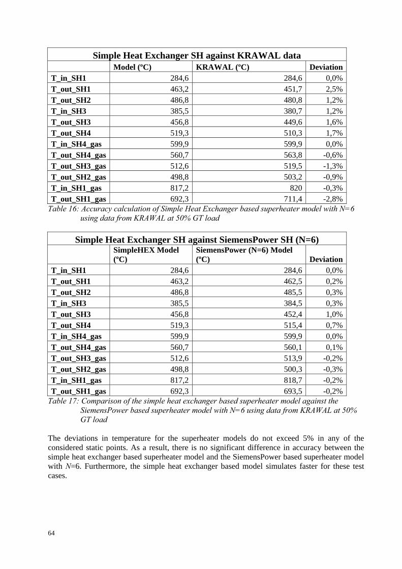
Simple Heat Exchanger SH against KRAWAL data Model (ºC) KRAWAL (ºC) DeviationT_in_SH1 284,6 284,6 0,0%T_out_SH1 463,2 451,7 2,5%T_out_SH2 486,8 480,8 1,2%T_in_SH3 385,5 380,7 1,2%T_out_SH3 456,8 449,6 1,6%T_out_SH4 519,3 510,3 1,7%T_in_SH4_gas 599,9 599,9 0,0%T_out_SH4_gas 560,7 563,8 -0,6%T_out_SH3_gas 512,6 519,5 -1,3%T_out_SH2_gas 498,8 503,2 -0,9%T_in_SH1_gas 817,2 820 -0,3%T_out_SH1_gas 692,3 711,4 -2,8%

Table 16: Accuracy calculation of Simple Heat Exchanger based superheater model with N=6 using data from KRAWAL at 50% GT load

Simple Heat Exchanger SH against SiemensPower SH (N=6)

SimpleHEX Model (ºC)

SiemensPower (N=6) Model (ºC) Deviation

T_in_SH1 284,6 284,6 0,0%T_out_SH1 463,2 462,5 0,2%T_out_SH2 486,8 485,5 0,3%T_in_SH3 385,5 384,5 0,3%T_out_SH3 456,8 452,4 1,0%T_out_SH4 519,3 515,4 0,7%T_in_SH4_gas 599,9 599,9 0,0%T_out_SH4_gas 560,7 560,1 0,1%T_out_SH3_gas 512,6 513,9 -0,2%T_out_SH2_gas 498,8 500,3 -0,3%T_in_SH1_gas 817,2 818,7 -0,2%T_out_SH1_gas 692,3 693,5 -0,2%

Table 17: Comparison of the simple heat exchanger based superheater model against the SiemensPower based superheater model with N=6 using data from KRAWAL at 50% GT load

The deviations in temperature for the superheater models do not exceed 5% in any of the considered static points. As a result, there is no significant difference in accuracy between the simple heat exchanger based superheater model and the SiemensPower based superheater model with N=6. Furthermore, the simple heat exchanger based model simulates faster for these test cases.

64

5.1.1.2 Verification of the Economizer The economizer is verified statically in the same manner as the superheater verification was performed in the previous section. The SiemensPower model with N=6 is used since it has comparable simulation time with the simple heat exchanger model. The test case uses constant incoming feedwater flow that has the same specific enthalpy and mass flow rate as the heat balance data from KRAWAL, data which is used for comparison in each of the three GT load cases. The heat transfer coefficient is tuned using the KRAWAL data at 70% gas turbine load. Then the same setup is used for the other two cases, namely 100% GT load and 50% GT load. 5.1.1.2.1 Investigating the Accuracy of Economizer Models at 70% GT load Table 18-20 present the results of the temperature comparisons for the SiemensPower based economizer model and the simple heat exchanger based economizer model with KRAWAL data. The temperatures in and out of the economizer on both the water and gas sides at steady state at 70% GT load are compared.

SiemensPower Heat Exchanger ECO (N=6) against KRAWAL data Model (ºC) KRAWAL (ºC) DeviationT_in_ECO 106,5 106,4 0,1%T_out_ECO 220,8 226,1 -2,4%T_in_ECO_gas 310,5 310,5 0,0%T_out_ECO_gas 145,1 150,4 -3,6%

Table 18: Accuracy calculation of the SiemensPower based economizer model using data from KRAWAL at 70% GT load

Simple Heat Exchanger ECO against KRAWAL data

Model (ºC) KRAWAL (ºC) DeviationT_in_ECO 106,4 106,4 0,0%T_out_ECO 221,6 226,1 -2,0%T_in_ECO_gas 310,5 310,5 0,0%T_out_ECO_gas 144,9 150,4 -3,8%

Table 19: Accuracy calculation of the simple heat exchanger based economizer model using data from KRAWAL at 70% GT load

Simple Heat Exchanger ECO against SiemensPower Heat Exchanger ECO (N=6)

SimpleHEX Model (ºC)

SiemensPower (N=6) Model (ºC) Deviation

T_in_SH1 106,4 106,5 0,0%T_out_SH1 221,6 220,8 0,4%T_out_SH2 310,5 310,5 0,0%T_in_SH3 144,9 145,1 -0,1%

Table 20: Comparison of the simple heat exchanger based economizer model and the SiemensPower based economizer model at 70% GT load

65

5.1.1.2.2 Investigating the Accuracy of Economizer Models with 100% GT load Table 21-23 present the results of the temperature comparisons for the SiemensPower based economizer model and the simple heat exchanger based economizer model with KRAWAL data at 100% GT load.

SiemensPower Heat Exchanger ECO (N=6) against KRAWAL data Model (ºC) KRAWAL (ºC) DeviationT_in_ECO 106,4 106,5 -0,1%T_out_ECO 224,1 230,3 -2,8%T_in_ECO_gas 324,6 324,6 0,0%T_out_ECO_gas 155,9 160 -2,6%

Table 21: Accuracy calculation of the SiemensPower based economizer model and data from KRAWAL at 100% GT load

Simple Heat Exchanger ECO against KRAWAL data

Model (ºC) KRAWAL (ºC) DeviationT_in_ECO 106,33 106,5 -0,2%T_out_ECO 222,92 230,3 -3,3%T_in_ECO_gas 324,6 324,6 0,0%T_out_ECO_gas 157,85 160 -1,4%

Table 22: Accuracy calculation of the simple heat exchanger based economizer model and data from KRAWAL at 100% GT load

Simple Heat Exchanger ECO against SiemensPower Heat Exchanger ECO (N=6)

SimpleHEX Model (ºC)

SiemensPower (N=6) Model (ºC) Deviation

T_in_ECO 106,33 106,4 0,0%T_out_ECO 222,92 224,1 -0,5%T_in_ECO_gas 324,6 324,6 0,0%T_out_ECO_gas 157,85 155,9 1,2%

Table 23: Comparison of the simple heat exchanger based economizer model and the SiemensPower based economizer model at 100% GT load

66

5.1.1.2.3 Investigating the Accuracy of Economizer Models at 50% GT load Table 24-26 present the results of the temperature comparisons for the SiemensPower based economizer model and the simple heat exchanger based economizer model with KRAWAL data at 50% GT load.

SiemensPower Heat Exchanger ECO (N=6) against KRAWAL data Model (ºC) KRAWAL (ºC) DeviationT_in_ECO 106,2 106,2 0,0%T_out_ECO 205,5 210 -2,2%T_in_ECO_gas 297,4 297,4 0,0%T_out_ECO_gas 135,6 140,7 -3,8%

Table 24: Accuracy calculation of the SiemensPower based economizer model and data from KRAWAL at 50% GT load

Simple Heat Exchanger ECO against KRAWAL data

Model (ºC) KRAWAL (ºC) DeviationT_in_ECO 106,2 106,2 0,0%T_out_ECO 207,1 210 -1,4%T_in_ECO_gas 297,4 297,4 0,0%T_out_ECO_gas 134,0 140,7 -5,0%

Table 25: Accuracy calculation of the simple heat exchanger based economizer model and data from KRAWAL at 50% GT load

Simple Heat Exchanger ECO against SiemensPower Heat Exchanger ECO (N=6)

SimpleHEX Model (ºC)

SiemensPower (N=6) Model (ºC) Deviation

T_in_ECO 106,2 106,2 0,0%T_out_ECO 207,1 205,5 0,7%T_in_ECO_gas 297,4 297,4 0,0%T_out_ECO_gas 134,0 135,6 -1,2%

Table 26: Comparison of the simple heat exchanger based economizer model and the SiemensPower based economizer model at 50% GT load

The deviations in temperature for the economizer models do not exceed 5% in any of the compared static points. Notable is that the deviations in temperature are quite large for the heat transfer coefficient design case, the ones at 70% GT load at the gas side. The heat transfer is concluded to be quite inaccurate when using a very large heat exchanger model, such as the ones used for this economizer. There is no significant difference in accuracy between the two models. The simple heat exchanger based model simulates faster for these test cases.

67

5.1.2 Verification of the Drum Boiler Core Model The Drum Boiler Core model has been subject to several tests and the theoretical models in [18] have been used as reference when interpreting the test results obtained from the performed simulations. The simulation results have been inspected for consistency and compliance with the expected physical behavior of the components.

5.1.2.1 The Test Bench for the Drum Boiler Core Model In Figure 35, the layout of the test bench in Dymola used for the drum boiler core model is shown.

Figure 35: The test bench for the Drum Boiler Core model

The idea with the bench is that different input disturbances in for example the heat flow, Q , or the feed water mass flow, qf , can be applied easily by connecting the desired input to the prepared test case. That simplifies the testing process, allowing multiple tests to be performed without rebuilding the whole setup for each test case.

68

5.1.2.2 Dynamic Test Cases for the Drum Boiler Core Model The tests of the dynamics of the model are all performed in Dymola with the help of the test bench described previously, although the setup differs a little depending on what disturbance the system is exposed to. Each of the test cases introduces disturbances in different inputs in order to examine how the drum boiler reacts to them. The inputs worth investigating are heat flow to the risers, feed water flow rate and steam flow rate. The outputs that are of interest when studying the results of each of the respective simulation results are mainly the drum level and the drum pressure, but the effect from the disturbances on other variables can also be interesting to evaluate in some cases. The goal of the tests is to examine the dynamic behavior of the model and the performance of the drum boiler controller. 5.1.2.2.1 Disturbance in Heat Flow without Controller When the exhaust gas from the GT varies in temperature and mass flow rate it is important to know what happens to the drum boiler. When the controller is removed and a stepwise disturbance is introduced to the heat flow, see Figure 36, many aspects in the dynamic behavior of the drum can be investigated. In this test case, a stepwise disturbance is introduced to the heat flow into the risers. The step is taken from the nominal value 40 MW and it is 25 MW so the final heat flow Q is 65 MW. The positive step in heat flow acts upon the drum boiler at time t=5000s. Time, measured in seconds, is on the x-axis in Figure 36-57.

Figure 36: A disturbance in the form of a positive step in the heat flow into the risers is

introduced In Figure 37, the temperature at the inlet and outlet of the drum is shown. When the step in heat flow is introduced, the temperature at the outlet of the drum quickly rises.

Figure 37: The temperature at the drum inlet (blue) and outlet (red)

The mass flow rate of the steam flowing out of the drum increases. This is because the additional heat increases the production of steam. This can be seen in Figure 38.

69

Figure 38: The feed water mass flow rate (blue) and steam mass flow rate (red)

Since the drum is not pressure controlled, the pressure inside the drum rises as seen in Figure 40. This makes the difference between the pressure in the inlet source of feed water and the drum smaller so the feed water mass flow rate in to the drum lowers as seen on the blue plot in Figure 38. The drum is subject to the shrink and swell phenomenon described in Section 3.4.6.2, which makes the level initially rise a bit before it sinks. Notice that without a controller connected, the level surpasses the lowest allowable level after approximately 160 s. The lowest allowable level is marked with green in Figure 39 below.

Figure 39: The drum level (blue) with the references highest allowed level (red) and lowest

allowed level (green) indicated The pressure inside the drum boiler rises because of the additional heat. This is caused by the increased steam production.

Figure 40: The pressure inside the drum boiler

70

The increase in the steam production consequently leads to a change in the distribution between the volume of steam and the volume of water inside the drum boiler, see Figure 41 below.

Figure 41: The total volume of steam (blue) and water (red)

There is also a change in the amount of steam produced in the risers. The factor that measures this, the volume fraction of steam in the risers, is quickly increased and it is shown in Figure 42 below.

Figure 42: The volume fraction of steam in the risers

Now, a negative step in the heat flow is instead introduced to the uncontrolled Drum Boiler Core model. The step is taken from the nominal value 40 MW and it is 25 MW so the final heat flow

is 15 MW, see QFigure 43 below.

71

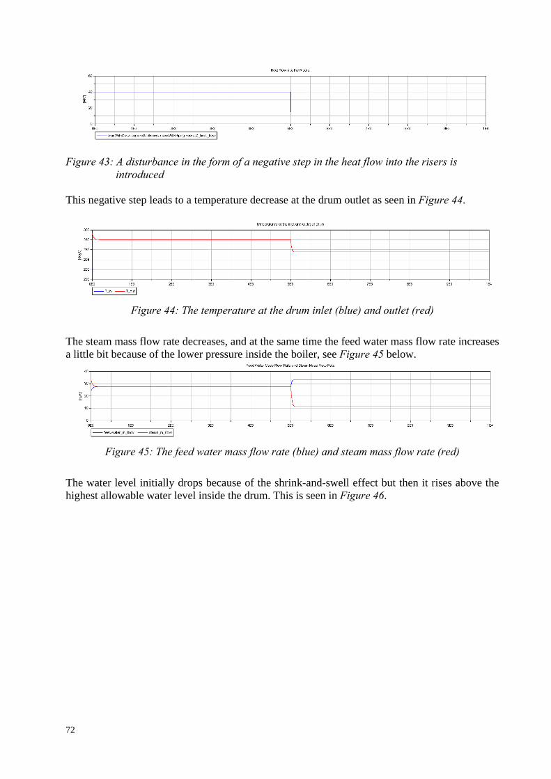
Figure 43: A disturbance in the form of a negative step in the heat flow into the risers is

introduced This negative step leads to a temperature decrease at the drum outlet as seen in Figure 44.

Figure 44: The temperature at the drum inlet (blue) and outlet (red)

The steam mass flow rate decreases, and at the same time the feed water mass flow rate increases a little bit because of the lower pressure inside the boiler, see Figure 45 below.

Figure 45: The feed water mass flow rate (blue) and steam mass flow rate (red)

The water level initially drops because of the shrink-and-swell effect but then it rises above the highest allowable water level inside the drum. This is seen in Figure 46.

72

Figure 46: The drum level (blue) with the references highest allowed level (red) and lowest

allowed level (green) indicated The pressure inside the drum boiler drops, see Figure 47.

Figure 47: The pressure inside the drum boiler

Consequently, the volume of the steam and water inside the drum redistributes as seen in Figure 48 below.

73

Figure 48: The total volume of steam (blue) and water (red)

The volume fraction of steam in the risers decreases since the boiling of the water in the riser tubes is reduced when the heat input is lowered, see Figure 49.

Figure 49: The volume fraction of steam in the risers

5.1.2.2.2 Disturbance in Heat Flow with Control In this test case, the drum has level and pressure control and the disturbance in heat flow is introduced to see how the controller performs. The Drum Boiler Core model is subject to a positive step in the heat flow to the risers as seen in Figure 50.

74

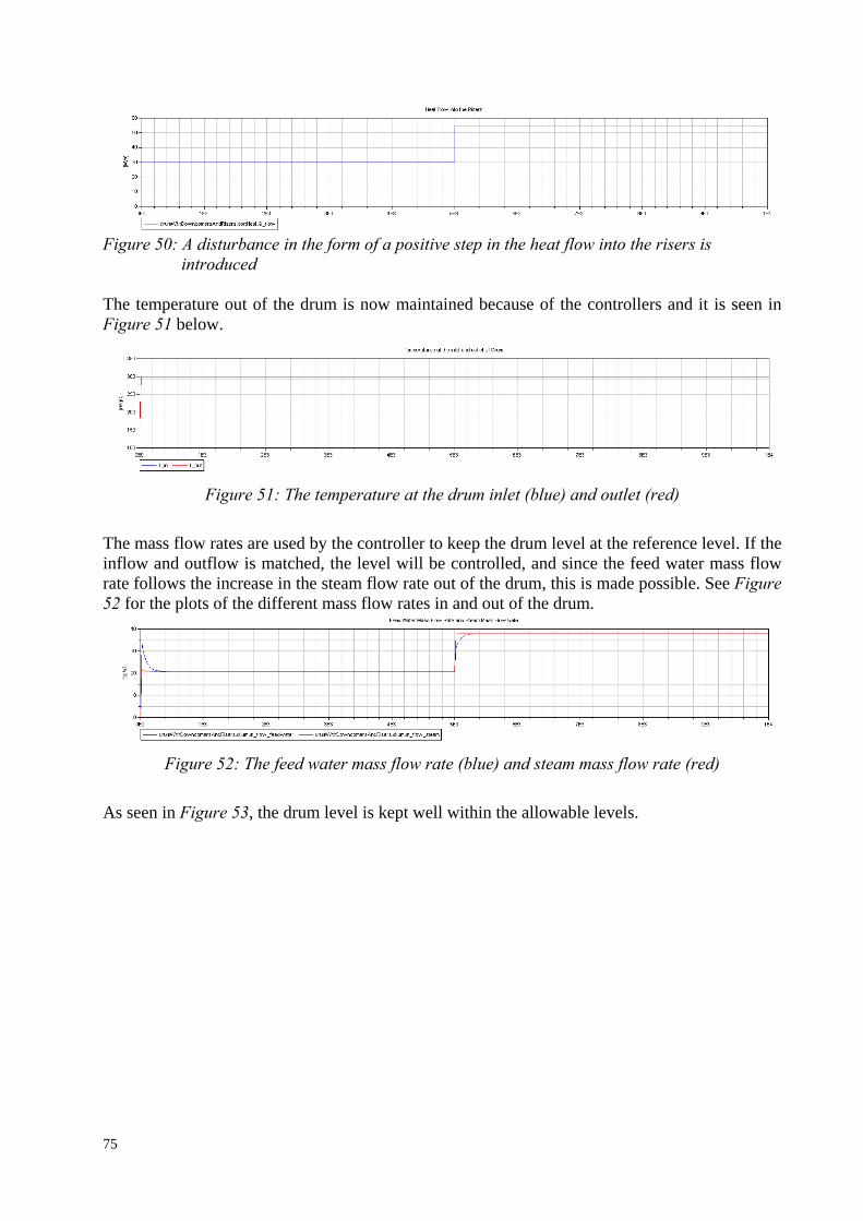
Figure 50: A disturbance in the form of a positive step in the heat flow into the risers is

introduced The temperature out of the drum is now maintained because of the controllers and it is seen in Figure 51 below.

Figure 51: The temperature at the drum inlet (blue) and outlet (red)

The mass flow rates are used by the controller to keep the drum level at the reference level. If the inflow and outflow is matched, the level will be controlled, and since the feed water mass flow rate follows the increase in the steam flow rate out of the drum, this is made possible. See Figure 52 for the plots of the different mass flow rates in and out of the drum.

Figure 52: The feed water mass flow rate (blue) and steam mass flow rate (red)

As seen in Figure 53, the drum level is kept well within the allowable levels.

75

Figure 53: The drum level (blue) with the references highest allowed level (red) and lowest

allowed level (green) indicated The pressure inside the drum boiler is controlled as seen in Figure 54.

Figure 54: The pressure inside the drum boiler

The steam and water volumes inside the drum boiler only varies a little bit because of the faster change of steam mass flow rate at the time for the step as seen in Figure 52. See Figure 55 for the plots of these volumes.

Figure 55: The total volume of steam (blue) and water (red)

76

The increase of heat that the riser tubes are subject to makes the fraction of steam in the risers larger as seen in Figure 56 below.

Figure 56: The volume fraction of steam in the risers

These test cases were also used to verify that the simulation times for the model were acceptable. When performing a simulation in Dymola, the user is automatically supplied with statistics regarding the simulation in a log file when the simulation has been performed. For a non controlled Drum Boiler model simulated for 10 000 s the simulation takes 0.641 s. For a controlled it takes 1.17 s. These simulation times are good; they are well within the ranges of acceptable simulation times. In Appendix B – Simulation Statistics, more details about how the simulations were performed are presented.

5.1.3 Verification of HRSG Superheater Temperature Controller Output One method of verifying the complete HRSG model, including an economizer, a controlled drum boiler and a controlled superheater, is to study the spray flow governed by the superheater temperature controller. The spray flow of the HRSG model running in steady state is compared with spray flow data in KRAWAL. The test is run for an HRSG without supplementary firing with input from a GT operating at 100% load. Results from the test are shown in Table 27 below.

Superheater Temperature Controller Spray Flow Comparison HRSG Model KRAWAL Unit p_steam_after_spray 61,02 60,92 bar h_steam_after_spray 3,29e3 3,30e3 kJ/kg m_flow_steam_SH 15,856 14,648 kg/s T_steam 444,2 448,6 ºC T_gas 502,6 513,3 ºC m_flow_spray 1,818 1,573 kg/s

Table 27: The results from the HRSG verification. Deviations of varying size between the model and KRAWAL date can be observed.

77

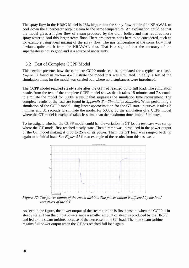
The spray flow in the HRSG Model is 16% higher than the spray flow required in KRAWAL to cool down the superheater output steam to the same temperature. An explanation could be that the model gives a higher flow of steam produced by the drum boiler, and that requires more spray water to cool this larger steam flow. There are uncertainties here to be considered, such as for example using ideal mixing of the spray flow. The gas temperature at the spray flow inlet deviates quite much from the KRAWAL data. That is a sign of that the accuracy of the superheater is not so good and is a source of uncertainty.

5.2 Test of Complete CCPP Model This section presents how the complete CCPP model can be simulated for a typical test case. Figure 33 found in Section 4.6 illustrate the model that was simulated. Initially, a test of the simulation times for the model was carried out, where no disturbances were introduced. The CCPP model reached steady state after the GT had reached up to full load. The simulation results from the test of the complete CCPP model shows that it takes 15 minutes and 7 seconds to simulate the model for 5000s, a result that surpasses the simulation time requirement. The complete results of the tests are found in Appendix B – Simulation Statistics. When performing a simulation of the CCPP model using linear approximation for the GT start-up curves it takes 3 minutes and 31 seconds to simulate the model for 5000s. So the simulation of a CCPP model where the GT model is excluded takes less time than the maximum time limit at 5 minutes. To investigate whether the CCPP model could handle variation in GT load a test case was set up where the GT-model first reached steady state. Then a ramp was introduced in the power output of the GT model making it drop to 25% of its power. Then, the GT load was ramped back up again to its initial load. See Figure 57 for an example of the results from this test case.

Figure 57: The power output of the steam turbine. The power output is affected by the load

variations of the GT As seen in the figure, the power output of the steam turbine is first constant when the CCPP is in steady state. Then the output lowers since a smaller amount of steam is produced by the HRSG and led to the steam turbine, because of the decrease in the GT load. Then the steam turbine regains full power output when the GT has reached full load again.

78

6 Discussion This chapter is used for discussion of the different stages and steps taken in the work with this thesis. The discussion starts with some remarks concerning the method used, then the model development process is commented. Finally, the model verification and documentation of the results are commented. Keeping the planning of the model development flexible was a good idea. When the model development phase began, it was clear that building fluid models in Dymola is an unpredictable and sometimes difficult task. Different issues when coding equations, tuning model parameters, and making the models integrate have been time-consuming parts of the development process. These issues made it nearly impossible to plan when to reach certain milestones. This was something that generated insecurity during the work with the thesis regarding what final results would be obtained in the end. One can actually argue that problems like this are natural parts of working in the field of modelling and simulation.

6.1 Discussion of the Model Development Method Different aspects of using the stepwise method, that was described in Section 2.1, and used when working with this thesis are discussed and evaluated in Sections 6.1.1-6.1.5 below.

6.1.1 Step 1: Information retrieval and requirement investigation Retrieving relevant information about the components and the models was of varying difficulty. Searching databases for academic papers gave useful information about the theoretical part and other sources of information were also helpful. Reading manuals and questioning Siemens employees gave information about the practical model development.

6.1.2 Step 2: Existing model investigation This step was sometimes more difficult than expected due to inadequate documentation of the existing models. Sources and motivation for the usage of equations and the assumptions made were not present in most cases. The strategy was to prioritize using component models and connections from the MSL to ensure that every part of the developed model is compatible, openly documented and available. Usage of the SiemensPower library also resulted in useful information for the model development.

6.1.3 Step 3: Model development During the model development, focus shifted a little from building models one by one to instead focus on building a complete functioning system for the whole combined cycle. Focusing on a step-wise model development and using the top-down approach turned out to be a good strategy since a CCPP model which is possible to simulate and reach steady state could be built. If much more details would have been incorporated initially for the separate models, there is a much higher probability of encountering difficulties when integrating these components to a functioning CCPP model. The development of the heat exchanger model was an example of where a detailed model was tested at first, but then difficulties when simulating the models were encountered when several

79

heat exchanger models were interconnected. That led to the development of the simplified heat exchanger model that is used in the HRSG model. But now, when the complete model functions, it is easier to test where details in for example flows and heat transfer can be incorporated, but still making sure that this is done without affecting the simulation times too much. One of the notable difficulties encountered when building the CCPP model was integrating the controllers and making them work simultaneously without loosing performance and risk the chattering phenomenon. The model is sometimes sensitive for larger changes in certain controller parameters, something that is not unusual. Studying the setup and parameters of an actual control system for a power plant would have helped to better establish in what region each of the controllers parameters should be. When building the models and discussing with my tutor at Siemens, it was discovered that the placement of valve-type models and volume-type models is very important when building fluid models in Dymola. They need to be alternated, so two models of the same kind should not be directly connected, cause that leads to simulation problems without any explanatory warning messages during compilation. This is something that should be pointed out more clearly in the Dymola manual.

6.1.4 Step 4: Model verification There are different ways to perform a verification of a developed model. Every verification method has its advantages and disadvantages. One method is to verify using available measurements from the actual component that is to be modeled. But getting that data is often a complicated and possibly expensive process. Even if good fit to measurement data is achieved, there are many questions to consider. Is the sample rate high enough? Where are the sensors placed, and what are the uncertainties of those measurements? What are the operating circumstances when doing the measurements? But this verification method is still the preferable, if executed properly, since it of course is directly based on measuring the properties of the physical components. Another method is to compare the simple models to more accurate and detailed models. Curves and parameters can then be fitted to match the more detailed models and still keep faster simulation times. This is a method that was used for the heat exchangers when modelling the heat transfer. They were compared to heat exchangers in the SiemensPower library. The results showed that the model was very similar to the SiemensPower model, with a little better execution time when running those test cases. Additionally, static points were compared to data from KRAWAL, a program using detailed component descriptions and equations to produce its results. The comparison showed that the model accuracy should be improved by using a better description of the heat transfer in a wider operating range. The third method is the one that has been used for verification of the drum boiler model. This involves verification by using equations for the models that are widely accepted and trustworthy. To ensure that the equations have been properly implemented in to a working model, one needs to perform several smaller experiments changing the inputs and the parameters and study if the outcome is the same as what to expect from theory and from experience. One can always discuss the correctness of the results when using this method since it is more of an experimental and pragmatic approach of verifying a model compared to using measurement data.

80

6.1.5 Step 5: Model documentation Documenting the models and the test results were done in a simple way using the documentation features in Dymola. The models based on the simple heat exchanger described in Section 4.1 are not yet properly documented in the Dymola model.

81

7 Conclusions and Future Work In this chapter the main results and conclusions are presented. Then some ideas for future work with the models are presented both with a short and also a longer time perspective.

7.1 Conclusions The main results and conclusions from the work with this thesis were the following:

• An efficient model of the HRSG and its control system has been developed.

• Model parameters have been tuned using heat balance data from KRAWAL so dimensions and medium properties are represented with certain accuracy at a number of reference points.

• The developed models are compatible with GT model & ST model from the

SiemensPower library and also with two newly developed condenser models.

• An operational model of a complete CCPP has been built. This was done integrating the developed models during the work with this thesis together with adaptations of already developed models.

• Steady state for the CCPP model is achieved during simulation and various disturbances

can then be introduced and studied. The models can also be used to study the performance of different control systems and control strategies.

• The requirement on maximum simulation time for a typical test case is fulfilled when

using linear functions to approximate the GT start-up curves.

7.2 Future Work Suggestions for future work are presented here, both short term improvements and suggestions for further model development in the long term. Short term:

• The feed water tank model and its control system should be more detailed and the ideal

heat source should be replaced with an extraction flow of hot water from the steam turbine.

• Adding the possibility to simulate the ST bypass system.

• Improve the superheater and economizer dynamics so that it better captures the time

aspect of heat up and transportation of steam through the superheater piping. Then the superheater steam temperature controller should better represent the real controller by modelling control logic for enthalpy and mass flow rate control.

82

• Improving the superheaters and the economizer models to better capture detailed behavior in these components. This by for example taking into account the appearance of flow regions and complicated response to the spray injection in the superheater model.

• Improving the model for the supplementary firing to capture for example the

consequences for the gas composition.

• More extensive verification of the models at different loads and during different scenarios. A lot of work remains in order to model a complete CCPP that can guarantee validity in the simulation results over a wide operating range.

Long term:

• Investigate the possibilities for modelling using simpler media functions such as for example Tabular Taylor Series Expansion for even shorter simulation times than when using the standard media functions found in MSL.

• Developing the models so that it can be used for simulation of start-up and shut-down

behavior. The next step would be to use it for making simulations for how to shorten the start-up times of the plant with usage of numerical optimization methods.

• Using these models for dynamic studies during the whole life-cycle of a plant, from

evaluating concepts to using it as a tool for maintenance and fault-tracing.

83

Bibliography [1] Q. Zhang; P.L. So. Dynamic Modelling of a Combined Cycle Plant for Power System

Stability Studies. Power Engineering Society Winter Meeting. 2000.

[2] P. Colonna; H. van Putten. Dynamic modeling of steam power cycles. Part I—Modeling paradigm and validation. Applied Thermal Engineering Volume 27, Issues 2–3. 2007.

[3] http://www.energy.siemens.com/. Power Generation. January 2012.

[4] SIT Internal Material

[5] http://www.3ds.com/products/catia/portfolio/dymola. Dymola. November 2011.

[6] www.modelica.org. Modelica. November 2011.

[7] Dymola User Manual – Dymola 7.0

[8] Damian Flynn. Thermal power plant simulation and control. ISBN 0-85296-419-6. IET. 2003.

[9] Yunus A. Cengel; Michael A. Boles. Thermodynamics: an engineering approach.

ISBN 0-07254-904-1. Mcgraw-Hill College. 2002.

[10] http://web.mit.edu. Thermodynamic Course Material. November 2011.

[11] Storck; Karlsson; Andersson; Loyd. Formelsamling i termo- och fluiddynamik.

[12] Henrik Alvarez. Energiteknik. ISBN 91-44-02894-6. Studentlitteratur. 2003.

[13] Marie-Noëlle Dumont; Georges Heyen. Mathematical modelling and design of an advanced once-through heat recovery steam generator. Computers & Chemical Engineering Volume: 28, Issue: 5, pp. 651-660. 2004.

[14] Meherwan P. Boyce. Handbook for cogeneration and combined cycle power plants. ISBN 07-91801-69-1. ASME Press, The American Society of Mechanical Engineers. 2001.

[15] Rolf Kehlhofer; Bert Rukes; Frank Hannemann; Franz Stirnimann. Combined-cycle gas & steam turbine power plants. ISBN 1-59370-168-3. PennWell Corp. 2009.

[16] P. Pourbeik. Modelling of Combined-Cycle Power Plants for Power System Studies. Power Engineering Society General Meeting Vol. 3 pp. 308 – 1313. 2003.

[17] V.Ganapathy. Heat-Recovery Steam Generators: Understand the Basics.

Chemical Engineering Progress. 1996.

[18] K. J. Åström; R.D. Bell. Drum-boiler dynamics. Automatica 36, pp. 363-378. 2000.

[19] R.A. Naghizadeh; B. Vahidi; M.R.B. Tavakoli. Estimating the Parameters of Dynamic Model of Drum Type Boilers Using Heat Balance Data as an Educational Procedure. Power Systems, IEEE Transactions Vol. 26 Issue 2 pp. 775-782. 2011.

[20] V.Ganapathy. Superheaters: design and performance. Hydrocarbon Processing. 2001.

[21] Faridah Mohamad Idris; Rubiyah Yusof; Marzuki Khalid. Modelling of A Superheater for A Combined Cycle Power Plant. Proceedings TENCON vol.3 pp. 518 - 523. 2000.

[22] C.X. Lu; N.W. Rees; S.C. Donaldson. The use of the Åström-Bell model for the design of drum level controllers in power plant boilers. World Congress, Vol. 16 Part 1. 2005.

84

85

[23] www.woodward.com/pdf/ic/83403.pdf. Industrial Steam Turbine Control, Woodward. 1992.

[24] Advanced Control of Steam Superheat Temperature on a Utility Boiler. ISA. 2000.

[25] P. Colonna; H. van Putten. Dynamic modeling of steam power cycles: Part II – Simulation of a small simple Rankine cycle system. Applied Thermal Engineering Vol. 27, Issues 14-15, pp. 2566-2582. 2007.

[26] E.J. Adam; J.L. Marchetti. Dynamic simulation of large boilers with natural recirculation. Computers and Chemical Engineering 23, pp. 1031-1040. 1999.

[27] T. Glad; L. Ljung. Reglerteknik - grundläggande teori. ISBN 9-14417-891-3. Studentlitteratur. 2006.

[28] D. H. Cooke. Modeling of off-design multistage turbine pressures by Stodola’s ellipse. Energy Incorporated PEPSE user’s group meeting Richmond Virginia. 1983.

References - Figures Figure 1 http://en.wikipedia.org/wiki/File:Brayton_cycle.svg. December 2011.

Figure 2 http://en.wikipedia.org/wiki/File:Rankine_cycle_layout.png. December 2011.

Figure 3 http://en.wikipedia.org/wiki/File:Rankine_cycle_Ts.png. December 2011.

Figure 4 http://www.secshellandtube.com/. December 2011.

Figure 5 Reference [15]. Modified by thesis author

Figure 6 http://www.energy.siemens.com/hq/en/power-generation/power-plants/gas-fired-power-plants/combined-cycle-power-plant-concept/. December 2011.

Figure 7 SIT internal material

Figure 11 http://blog.opticontrols.com/archives/date/2010/07. Modified by thesis author, December 2011.

Figure 12 http://blog.opticontrols.com/archives/date/2010/07. Modified by thesis author, December 2011.

Figure 13 http://www.sit-ab.se/03_produkter_losningar.html. December 2011.

Figure 14 http://www.energy.siemens.com/hq/en/power-generation/steam-turbines/sst-600.htm#content=Benefits. December 2011.

Figure 15 SIT internal material

Appendix A – Tables of Variables and Parameters

Variables Risers

Variable Dymola code notation Unit Description Er Er [J] Energy in risers hs h_saturated_steam [J/kg] Specific enthalpy of steam hw h_saturated_liquid [J/kg] Specific enthalpy of liquid Mw,risers M_liquid_risers [kg] Liquid mass in risers Ms,risers M_steam_risers [kg] Steam mass in risers Mr Mr [kg] Total mass of risers p p [Pa] Pressure inside risers ρw rho_liquid [kg/m3] Density in liquid phase ρs rho_steam [kg/m3] Density in steam phase ts T_saturated_steam [K] Temperature saturated steam Q Q_heat_flow [W] Heat flow rate qdc m_flow_downcomers [kg/s] Mass flow rate from downcomers qr m_flow_risers [kg/s] Mass flow rate to drum Vw,risers V_liquid_risers [m3] Volume of liquid in risers Vs,risers V_steam_risers [m3] Volume of steam in risers

Drum Variable Dymola code notation Unit Description

E t Et [J] Total energy hf h_feedwater [J/kg] Enthalpy feed water hw h_saturated_liquid [J/kg] Enthalpy saturated liquid hs h_saturated_steam [J/kg] Enthalpy saturated steam Llvl_drum drumLevel [m] Drum level

86

Mdrum M_drum [kg] Mass in drum Mw,drum M_liquid_drum [kg] Liquid mass in drum Ms,drum M_steam_drum [kg] Vapor mass in drum Msd Msd [kg] Steam bubble mass Mt Mt [kg] Total mass p p [Pa] Pressure qcd m_flow_drum_cond [kg/s] Mass flow drum condensation qct m_flow_total_cond [kg/s] Mass flow total condensation qdc m_flow_downcomers [kg/s] Mass flow downcomers qf m_flow_feedwater [kg/s] Mass flow feed water qr m_flow_risers [kg/s] Mass flow risers qs m_flow_steam [kg/s] Mass flow steam qsd m_flow_drum_steam [kg/s] Mass flow drum steam ρw rho_liquid [kg/m3] Density liquid ρs rho_steam [kg/m3] Density steam ts T_saturated_steam [K] Temperature saturated steam Vwd V_drum_liquid [m3] Volume drum liquid Vsd V_drum_steam [m3] Volume drum steam under the liquid level Vwt V_total_liquid [m3] Volume total liquid Vst V_total_steam [m3] Volume total steam αr xr [-] Steam quality at the riser outlet

rvα xrv [-] Average volume fraction Table 28: List of the variables used in the drum boiler model

87

Parameters Downcomers

Parameter Dymola code notation Unit Description ddowncomers diameterDowncomers [m] Diameter of downcomers hdowncomers heightDowncomers [m] Height of downcomers ldowncomers lengthDowncomers [m] Length of downcomers Ndowncomers nParallelDowncomers [-] Number of identical parallel pipes in downcomers pa,start,downcomers p_a_startDowncomers [Pa] Start value pressure downcomers port a pb,start,downcomers p_b_startDowncomers [Pa] Start value pressure downcomers port b Qstart,downcomers m_flow_startDowncomers [kg/s] Start value mass flow rate downcomers Rdowncomers roughnessDowncomers [m] Surface roughness downcomers

Risers Parameter Dymola code notation Unit Description

drisers diameterRisers [m] Diameter of risers hrisers heightRisers [m] Height of risers lrisers lengthRisers [m] Length of risers Mmetal,risers m_metal_risers [kg] Metal mass risers Nrisers nParallelRisers [-] Number of identical parallel pipes in risers pa,start,risers p_a_startRisers [Pa] Start value pressure risers port a pb,start,risers p_b_startRisers [Pa] Start value pressure risers port b pstart,risers p_startRisers [Pa] Start value pressure inside risers qrisers m_flow [kg/s] Mass flow rate risers qstart,risers m_flow_startRisers [kg/s] Start value mass flow rate risers Rrisers roughnessRisers [m] Roughness surface risers Vrisers V_risers [m3] Volume risers

Circulation Pump Parameter Dymola code notation Unit Description

pa,nominal p_a_nominal [Pa] Nominal inlet pressure of circulation pump pb,nominal p_b_nominal [Pa] Nominal outlet pressure of circulation pump pa,start p_a_start [Pa] Guess value for inlet pressure for circulation pump pb,start p_b_start [Pa] Guess value for outlet pressure for circulation pump qnominal m_flow_nominal [kg/s] Nominal mass flow rate for circulation pump

88

89

qpump,downcomers-risers m_flow_pumpDowncomersRisers [kg/s] Nominal mass flow rate for downcomers-risers loop qstart m_flow_start [kg/s] Guess value of m_flow of circulation pump

Drum Parameter Dymola code notation Unit Description

Ad A_drum [m2] Area of the water surface in the drum β beta [-] Beta coefficient, empirical value in a equation describing the distribution of steam in the drum

Cp C_p [J/(kg.K)] Cp Specific heat capacity of the surrounding metal ddrum d_drum [m] Diameter cylindric drum ldrum l_drum [m] Length cylindric drum mmd m_metal_drum [kg] Metal mass drum mmt m_metal_total [kg] Metal mass total orientationdrum orientation_drum [-] The orientation of the drum, Horizontal: orientation_drum=1, Vertical: orientation_drum=2

pstart p_start [Pa] Start value pressure Td t_drum_steam [-] t drum steam, denotes the residence time of the steam in the drum Vdrum V_drum [m3] Drum volume Vsd,start V_drum_steam_start [m3] Start value of steam volume in drum Vt V_total [m3] Total volume Vwt,start V_total_liquid_start [m3] Start value of total liquid volume V0

sd V0_drum_steam [-] V0 drum steam, denotes the volume of steam in the drum if there would be no condensation

αr,start xr_start [-] Start value of xr, denotes the steam quality at the riser outlet αrv,start xrv_start [-] Start value of xrv, denotes the average volume fraction of steam

Table 29: List of the parameters used in the drum boiler model

Appendix B – Simulation Statistics Simulation Statistics for the Core Drum Boiler Model In Figure 58 below the core drum boiler model without controllers is presented. This is the setup used when measuring the simulation times.

Figure 58: A drum boiler with downcomers and risers that lacks the pressure controller and

level control The Dymola simulation log gives information about simulation, including the simulation times. The simulation time is affected by the sampling rate. When simulating for 10 000 s, the execution time is 0.641 s with 500 sampling points. When sampling 5000 points the model setup takes 4.03 s to simulate.

90

The setup used for measuring the simulation times of the controlled drum boiler model is presented in Figure 59 below.

Figure 59: A controlled drum boiler with downcomers and risers. A disturbance in the form of a

positive step in heat flow acts upon the drum boiler at time t=5000 s When simulating for 10 000 s, the execution time is 1.17 s with 500 sampling points. When sampling 5000 points the model setup takes 4.5 s to simulate.

91

Simulation Statistics for the CCPP Model

Here, simulation statistics provided by Dymola after a simulation of the complete CCPP model from start-up to steady state at 70 % load is presented. The setup used for this test is shown in Figure 60.

Figure 60: The complete CCPP model with the GT model coupled to the HRSG

When simulating the CCPP model and using the GT model for 5 000 s, the execution time is 907 s with 500 sampling points. When using linear approximation of the GT start-up curves the simulation takes 211 s with 500 sampling points.

92