Simulation of Greenhouse Climate Monitoring and Control
21
Sensors 2009, 9, 232-252; doi:10.3390/s90100232 sensors ISSN 1424-8220 www.mdpi.com/journal/sensors Article Simulation of Greenhouse Climate Monitoring and Control with Wireless Sensor Network and Event-Based Control Andrzej Pawlowski 1 , Jose Luis Guzman 1, *, Francisco Rodríguez 1 , Manuel Berenguel 1 , José Sánchez 2 and Sebastián Dormido 2 1 Department of Languages and Computation, University of Almería; Ctra. Sacramento s/n, 04120, Almería, Spain; E-Mails: [email protected]; [email protected]; [email protected] 2 Department of Computer Science and Automatic Control, UNED C/. Juan del Rosal, 16, 28040, Madrid, Spain; E-Mails: [email protected]; [email protected] * Author to whom correspondence should be addressed; E-Mail: [email protected]; Tel.: +34 950 015677; Fax: +34 950 015129. Received: 11 December 2008; in revised form: 31 December 2008 / Accepted: 5 January 2009 / Published: 8 January 2009 Abstract: Monitoring and control of the greenhouse environment play a decisive role in greenhouse production processes. Assurance of optimal climate conditions has a direct influence on crop growth performance, but it usually increases the required equipment cost. Traditionally, greenhouse installations have required a great effort to connect and distribute all the sensors and data acquisition systems. These installations need many data and power wires to be distributed along the greenhouses, making the system complex and expensive. For this reason, and others such as unavailability of distributed actuators, only individual sensors are usually located in a fixed point that is selected as representative of the overall greenhouse dynamics. On the other hand, the actuation system in greenhouses is usually composed by mechanical devices controlled by relays, being desirable to reduce the number of commutations of the control signals from security and economical point of views. Therefore, and in order to face these drawbacks, this paper describes how the greenhouse climate control can be represented as an event-based system in combination with wireless sensor networks, where low-frequency dynamics variables have to be controlled and control actions are mainly calculated against events produced by external disturbances. The proposed control system allows saving costs related with wear OPEN ACCESS
Transcript of Simulation of Greenhouse Climate Monitoring and Control

Sensors 2009, 9, 232-252; doi:10.3390/s90100232
sensors ISSN 1424-8220
www.mdpi.com/journal/sensors
Article
Simulation of Greenhouse Climate Monitoring and Control with Wireless Sensor Network and Event-Based Control
Andrzej Pawlowski 1, Jose Luis Guzman 1,*, Francisco Rodríguez 1, Manuel Berenguel 1,
José Sánchez 2 and Sebastián Dormido 2
1 Department of Languages and Computation, University of Almería; Ctra. Sacramento s/n, 04120,
Almería, Spain; E-Mails: [email protected]; [email protected]; [email protected] 2 Department of Computer Science and Automatic Control, UNED C/. Juan del Rosal, 16, 28040,
Madrid, Spain; E-Mails: [email protected]; [email protected]
* Author to whom correspondence should be addressed; E-Mail: [email protected];
Tel.: +34 950 015677; Fax: +34 950 015129.
Received: 11 December 2008; in revised form: 31 December 2008 / Accepted: 5 January 2009 /
Published: 8 January 2009
Abstract: Monitoring and control of the greenhouse environment play a decisive role in
greenhouse production processes. Assurance of optimal climate conditions has a direct
influence on crop growth performance, but it usually increases the required equipment
cost. Traditionally, greenhouse installations have required a great effort to connect and
distribute all the sensors and data acquisition systems. These installations need many data
and power wires to be distributed along the greenhouses, making the system complex and
expensive. For this reason, and others such as unavailability of distributed actuators, only
individual sensors are usually located in a fixed point that is selected as representative of
the overall greenhouse dynamics. On the other hand, the actuation system in greenhouses is
usually composed by mechanical devices controlled by relays, being desirable to reduce
the number of commutations of the control signals from security and economical point of
views. Therefore, and in order to face these drawbacks, this paper describes how the
greenhouse climate control can be represented as an event-based system in combination
with wireless sensor networks, where low-frequency dynamics variables have to be
controlled and control actions are mainly calculated against events produced by external
disturbances. The proposed control system allows saving costs related with wear
OPEN ACCESS

Sensors 2009, 9
233
minimization and prolonging the actuator life, but keeping promising performance results.
Analysis and conclusions are given by means of simulation results.
Keywords: Event-based control; Wireless Sensor Network, greenhouse climate control
1. Introduction
Nowadays, the agro-alimentary sector is incorporating new technologies due to the large production
demands and the diversity, quality, and market presentation requirements. A technological renovation
of the sector is being required where the control engineering plays a decisive role. Automatic control
and robotics techniques are incorporated in all the agricultural production levels: planting, production,
harvest, post-harvest processes, and transportation. Modern agriculture is subjected to regulations in
terms of quality and environmental impact, and thus it is a field where the application of automatic
control techniques has increased substantially during the last years [1-5].
As it is well-known, greenhouses have a very extensive surface where the climate conditions can
vary at different points (spatial distributed nature). Despite of that feature, it is very common to install
only one sensor for each climatic variable in a fixed point of the greenhouse as representative of the
main dynamics of the system. One of the reasons is that typical greenhouse installations require a large
amount of wire to distribute sensors and actuators. Therefore, the system becomes complex and
expensive and the addition of new sensors or actuators at different points in the greenhouses is thus
quite limited.
In the last years, Wireless Sensor Networks (WSN) are becoming an important solution to this
problem [6-7]. WSN is a collection of sensor and actuators nodes linked by a wireless medium to
perform distributed sensing and acting tasks [8]. The sensor nodes collect data and communicate over
a network environment to a computer system, which is called, a base station. Based on the information
collected, the base station takes decisions and then the actuator nodes perform appropriate actions
upon the environment. This process allows users to sense and control the environment from anywhere
[7]. There are many situations in which the application of the WSN is preferred, for instance,
environment monitoring, product quality monitoring, and others where supervision of big areas is
necessary [9]. In this work, WSN are used in combination with event-based systems to control the
inside greenhouse climate.
On the other hand, event-based systems are becoming increasingly commonplace, particularly for
distributed real-time sensing and control. A characteristic application running on an event-based
operating system is that where state variables will typically be updated asynchronously in time, for
instance, when an event of interest is detected or because of delay in computation and/or
communication [10]. Event-based control systems are currently being presented as solutions to many
control problems [10-13]. In event-based control systems, the proper dynamic evolution of the system
variables is what decides when the next control action will be executed, whereas in a time-based
control system, the autonomous progression of the time is what triggers the execution of control
actions. The fundamental reason for the predominance of the time-based control systems has been
based on the existence of a well established theory for control systems with a constant sampling time

Sensors 2009, 9
234
[14]. However, current distributed control systems also impose restrictions on the architecture of the
system that makes difficult the adoption of a paradigm based on events activated per time. For
instance, in the case of closed-loop control using computer networks or buses (such as field bus, local
network area, or Internet), where asynchronous communication is required. An alternative to these
approaches consists of using event-based controllers that are not restricted to the synchronous
occurrence of controller actions. The employment of synchronous sampling period is one of the
severest conditions that control engineers follow for implementation tasks. Many examples can be
found, such as mobile phones, printing devices, or PDA’s. The complexity of these devices
(processes), as well as the complexity of the controller, is increasing very fast. These requirements can
be reduced with event-based controllers, where the control actions can be executed in an asynchronous
way [15].
Control problems in greenhouses are mainly focused on fertirrigation and climate systems. The
fertirrigation control problem is usually solved providing the amount of water and fertilizers required
by the crop. The climate control problem consists in keeping the greenhouse temperature and humidity
in specific ranges despite of disturbances. Adaptive and feedforward controllers are commonly used
for the climate control problem. Therefore, fertirrigation and climate systems can be represented as
event-based control problems where control actions will be calculated and performed when required
by the system, for instance, when water is required by the crop or when ventilation must be closed due
to changes in outside weather conditions. Furthermore, such as discussed above, with event-based
control systems a new control signal is only generated when a change is detected in the system. That
is, the control signal commutations are produced only when events occur. This fact is very important
for the actuator life and from an economical point of view (reducing the use of electricity or fuel),
especially in greenhouses where commonly actuators are composed by mechanical devices controlled
by relays.
Therefore, this paper presents the combination of WSN and event-based control systems to be
applied in greenhouses. The main focus of this paper is therefore the presentation of a complex real
application where using a WSN, as an emerging technology and Event-Based Control, as a new
paradigm in process control, the following issues have been addressed:
the issues posed to a multivariable, interacting control system by possibly faulty
communications (as in a wireless context),
the location of sensors to correctly represent, for the purpose of control, spatially distributed
quantities,
the efficient use of actuators, the term “efficient” referring also to correct use and wear
minimization,
the effects of event-based sampling.
As a first approximation, event-based control has been applied for temperature and humidity control
issues. The main advantages of the proposed control problem in comparison with previous works is
that promising performance results are reached reducing the use of wire and the changes on the control
signals, what it is translated into reductions on costs and a longer actuator life. The ideas presented in
this paper could be easily extrapolated, for instance, to building automation.
The work is organized as follows. Section 2 is devoted to describe the greenhouse climate control
problem. Afterwards, the event-based system and WSN for the greenhouse temperature control is

Sensors 2009, 9
235
discussed. Simulations results are presented in section 4. Finally, some conclusions are given in
Section 5.
2. Greenhouse Climatic Control Problem
2.1. Description of the Climatic Control Problem
Crop growth is mainly influenced by the surrounding environmental climatic variables and by the
amount of water and fertilizers supplied by irrigation. This is the main reason why a greenhouse is
ideal for cultivation, since it constitutes a closed environment in which climatic and fertirrigation
variables can be controlled to allow an optimal growth and development of the crop. The climate and
the fertirrigation are two independent systems with different control problems. Empirically, the
requirements of water and nutrients of different crop species are known and, in fact, the first automated
systems were those that controlled these variables. As the problem of greenhouse crop production is a
complex issue, an extended simplification consists of supposing that plants receive the amount of
water and fertilizers that they require at every moment. In this way, the problem is reduced to the
control of crop growth as a function of climate environmental conditions [16, 17].
Figure 1. Climatic Control Variables.
The dynamic behavior of the greenhouse microclimate is a combination of physical processes
involving energy transfer (radiation and heat) and mass balance (water vapour fluxes and CO2
concentration). These processes depend on the outlet environmental conditions, structure of the
greenhouse, type and state of the crop, and on the effect of the control actuators [18]. The main ways
of controlling the greenhouse climate are by using ventilation and heating to modify inside
temperature and humidity conditions, shading and artificial light to change internal radiation, CO2
injection to influence photosynthesis, and fogging/misting for humidity enrichment. A deeper study
about the features of the climatic control problem can be found in [16].
Sensors 2009, 9
236
The approach presented in this paper is applied to the climatic conditions of mild winter in Southern
Europe (the data used for the simulations performed in this paper have been collected in a greenhouse
from Southeastern Spain), where the production in greenhouses is made without CO2 enrichment and
the demand of quality products is increasing every day. Considering the greenhouse structures, the
commonest actuators, the crop types, and the commercial conditions of this geographical area, the
main climate variables to control are the temperature and the humidity. The PAR (Photosynthetically
Active Radiation: it is the spectral range from 400 to 700 Wm2, which is used by the plants as energy
source in the photosynthesis process.) radiation is controlled with shade screens but its use is not much
extended. So, this paper is focused on the temperature and humidity control problems.
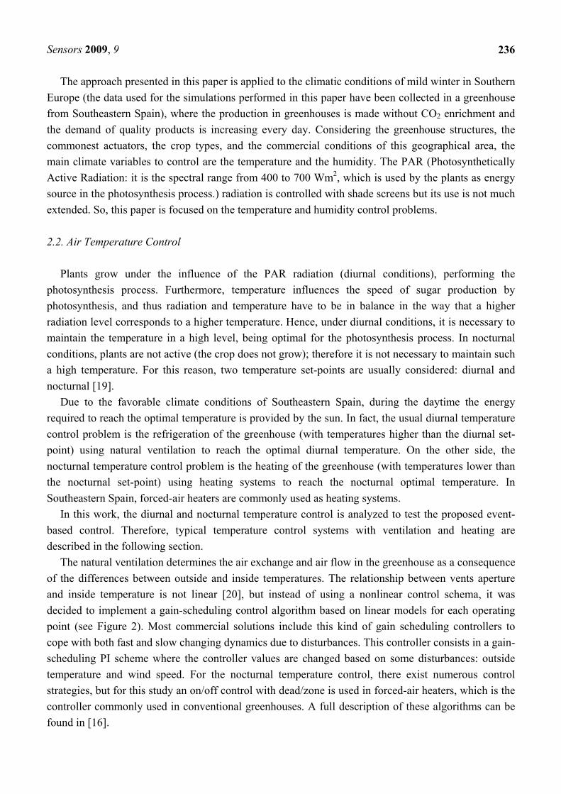
2.2. Air Temperature Control
Plants grow under the influence of the PAR radiation (diurnal conditions), performing the
photosynthesis process. Furthermore, temperature influences the speed of sugar production by
photosynthesis, and thus radiation and temperature have to be in balance in the way that a higher
radiation level corresponds to a higher temperature. Hence, under diurnal conditions, it is necessary to
maintain the temperature in a high level, being optimal for the photosynthesis process. In nocturnal
conditions, plants are not active (the crop does not grow); therefore it is not necessary to maintain such
a high temperature. For this reason, two temperature set-points are usually considered: diurnal and
nocturnal [19].
Due to the favorable climate conditions of Southeastern Spain, during the daytime the energy
required to reach the optimal temperature is provided by the sun. In fact, the usual diurnal temperature
control problem is the refrigeration of the greenhouse (with temperatures higher than the diurnal set-
point) using natural ventilation to reach the optimal diurnal temperature. On the other side, the
nocturnal temperature control problem is the heating of the greenhouse (with temperatures lower than
the nocturnal set-point) using heating systems to reach the nocturnal optimal temperature. In
Southeastern Spain, forced-air heaters are commonly used as heating systems.
In this work, the diurnal and nocturnal temperature control is analyzed to test the proposed event-
based control. Therefore, typical temperature control systems with ventilation and heating are
described in the following section.
The natural ventilation determines the air exchange and air flow in the greenhouse as a consequence
of the differences between outside and inside temperatures. The relationship between vents aperture
and inside temperature is not linear [20], but instead of using a nonlinear control schema, it was
decided to implement a gain-scheduling control algorithm based on linear models for each operating
point (see Figure 2). Most commercial solutions include this kind of gain scheduling controllers to
cope with both fast and slow changing dynamics due to disturbances. This controller consists in a gain-
scheduling PI scheme where the controller values are changed based on some disturbances: outside
temperature and wind speed. For the nocturnal temperature control, there exist numerous control
strategies, but for this study an on/off control with dead/zone is used in forced-air heaters, which is the
controller commonly used in conventional greenhouses. A full description of these algorithms can be
found in [16].

Sensors 2009, 9
237
Figure 2. Diurnal gain scheduling controller with temperature setpoint generator based on humidity.
2.3. Humidity Control
Water vapour inside the greenhouse is not one of the most important variables affecting the crop
growth. However, the humidity control has a special interest, because high humidity may produce the
appearance of diseases and decrease transpiration, and low humidity may cause hydric stress, closing
the stomata, and thus reducing the photosynthesis due to a decrease in the CO2 assimilation. There are
two problems involved in the humidity control: (1) the greenhouse inside temperature and the relative
humidity are inversely related when the greenhouse air not mixed with the external air, generally
colder and drier (when one of them increases the other one decreases and vice versa); (2) the same
actuators are used for controlling temperature and humidity. The temperature control has the main
priority because it affects to the crop growth directly. In order to keep the humidity within a
determined range, the temperature set-point can be changed based on the inside relative humidity
value. Hence, the humidity controller acts as a set-point generator being able to change the temperature
set-point in small ranges. The modification of the temperature set-point value depends on actual
humidity level, selecting a maximum allowable modification for a specific kind of crop. A lower
temperature set-point allows evacuating the humid air as a consequence of the exchange with the
outside air because it is drier than the internal air. However, a higher set-point provokes that the
ventilation remains closed for longer periods of time keeping the water vapour of air inside the
greenhouse, and so increasing the humidity [16-17].
3. WSN and Event-Based System for Greenhouse Climate Control
Before addressing the greenhouse climate control as an event-based control problem, some basic
notions about level crossing sampling and event-based control are introduced.
3.1. Level Crossing Sampling and Event-Based Control
As discussed above, in an event-based control system the control actions are executed in an
asynchronous way, that is, the sampling period is governed by system events and it is called event-
based sampling. The event-based sampling is a very old idea [21] and indicates that the most
appropriate method of sampling consists in transmitting information only when a significant change in
Greenhouse
AdaptiveMechanism
TemperatureController
Outside Temperature
+
Temperature
TemperatureSetpoint
Outside Wind Speed
-
NaturalVentilation
SetpointGenerator
Humidity
e u
Temperature Setpointbased on humidity Actuator + Plant
Greenhouse
AdaptiveMechanism
TemperatureController
Outside Temperature
+
Temperature
TemperatureSetpoint
Outside Wind Speed
-
NaturalVentilation
SetpointGenerator
Humidity
e u
Temperature Setpointbased on humidity Actuator + Plant

Sensors 2009, 9
238
the signal occurs justifying the acquisition of a new sample. During last years, researchers have
demonstrated special interest on this sampling technique [22-25]. This kind of sampling method has
received different names in the literature [15]: adaptive sampling, asynchronous delta-modulation,
dead-band method, send-on-delta method, level crossing sampling, and Lebesgue sampling.
In spite of these names (in this paper the name level crossing sampling is selected), the basic
principle is the same: the input signal is sampled when the absolute value of the difference between the
current value, x(ts), and the last sampled value of a signal, x(tk), is bigger than a specific limit δ:
sk txtx (1)
When the change in the signal is relatively small, the number of samples is significantly smaller than
in a periodic sampling scheme, such as shown in Figure 3.
Figure 3. Level crossing method.
�
y(t)
t
In an event-based system, the occurrence of an event, rather than the passing of the time, is what
decides when a sample should be taken. The nature of the event could vary. Examples could be those
as a measured signal crosses a certain limit or the arrival of a data packet to a node on a computer-
based network [11].
When the sampling is event-triggered, event-based control systems can be considered as alternative
for time-based control systems. Other names for these control systems are aperiodic or asynchronous
control systems. In a general way, an event-based controller consists of two parts: an event detector
and a controller. The event detector deals with indicating to the controller when a new control signal
must be calculated due to the occurrence of a new event. For instance, the decision to calculate a new
control signal could be if the absolute value of the difference between the current value of the error,
e(tk), and the value of the last error calculated, e(ts), is greater than a limit δ, or when the time elapsed
since the last sample, hact, exceeds a maximum limit hmax: sk tete and maxhtt sk (2)
From condition (2), the controller will be executed at the nominal sampling time hnom during
transients (for instance, set point changes and load disturbances) or if the time difference between
samples is bigger than the maximal sampling interval, hmax, during steady state conditions [11]. The
last condition, tk ts ≥ hmax, is a simple safety condition to ensure the control system stability due to
sampling problems.

Sensors 2009, 9
239
3.2. WSN and Event-Based Control in Greenhouses
As commented above, this paper is devoted to analyzing diurnal and nocturnal temperature control
with natural ventilation and heating systems, and humidity control as a secondary control objective.
Under diurnal conditions, the controlled variable is the inside temperature and the control signal is the
vent opening. The use of natural ventilation produces an exchange between the inside and outside air,
usually provoking a decrease in the inside temperature of the greenhouse. The controller must
calculate the necessary vent opening to reach the desired set-point. As discussed in Section 2, the
commonest controller used is a gain scheduling PI scheme where the controller parameters are
changed based on some disturbances: outside temperature and wind speed. In the case of nocturnal
temperature control, forced-air heaters are used to increase the inside temperature and an on/off control
with dead/zone was selected as heating controller.
Figure 4. Event-Based Control and WSN
Sensor3Zig
Bee
WSN
SensorN
Sensor2
Sensor1
Actuator3
ActuatorN
Actuator2
Actuator1
Controller
Event
Generator
GreenhouseEvent-Control System
In this work, the idea is to combine WSN with event-based control such as shown in Figure 4. The
sensors are distributed along the greenhouse including a level crossing sampling for each variable.
That is, the greenhouse is provided with a WSN where each sensor will transmit data if the absolute
value of the difference between the current value of the variable, v(tk), and the previous value of the
variable v(ts), is greater than a limit δ. Therefore, the first step in this work was to calculate suitable
limits δ for each greenhouse variable. Such as shown in next section, this limit has a direct influence
on the event generation and on the quantity of transmitted data.
Table 1. Limits for greenhouse variables.
Variable Limit (δ = 5%) Limit (δ = 3%)
Inside Temperature 0.60 0.36
Outside Temperature 0.61 0.36
Humidity 2 1.2
Solar Radiation 34.30 20.58
Wind Speed 0.53 0.31
Wind Direction 17.84 10.70

Sensors 2009, 9
240
Table 1 shows the individual limits for the commonest variables used for control purposes. These
limits of δ = 3% and δ = 5% were calculated based on the authors experience and after analyzing three
years of data. The calculation of δ limit for each individual variable was performed studying its
minimum and maximum values. The value of the change of each variable for δ = 3% and δ = 5% was
determined calculating the 3% and 5% of the difference between the maximum and minimum values.
Instead of choosing only one limit for each variable, these two different limits were evaluated to
analyze their effects, such as presented in next section.
On the other hand, the control system is now composed by an event generator plus the original
controllers. In this way, the gain scheduling and the on/off controllers will calculate a new control
action only when an event is detected by the event generator. The typical event is that when the
absolute value of the difference between the current value of the error, e(tk), and the value of the error
calculated previously, e(ts), is greater than a limit δ. In accordance with equation (2), transmission is
also made when the time elapsed since the last sample, hact, exceeds the limit hmax. Furthermore, and
such as commented above, the control depends on disturbances and other events will be also generated
by changes of the corresponding disturbances. The events from the disturbances will be detected by
the event generator according to the limits shown in Table 1. These events are analyzed in Section 4.
4. Simulation Results
4.1. Material and Methods
The simulations presented in this section have been performed using the greenhouse climatic model
developed by [16] and the TrueTime MATLAB/Simulink toolbox [26], [27].
As commented above, the dynamic behavior of the microclimate inside the greenhouse is a
combination of physical processes involving energy transfer (radiation and heat) and mass balance
(water vapor fluxes and CO2 concentration). The greenhouse climate model developed in [16]
capturates this dynamic behavior and it can be summarized as:
),,,,,( tCVPUXfdt
dX , ii XtX )(
where X = X(t) is a n1-dimensional vector of greenhouse climate state variables (mainly the inside air
temperature and humidity, CO2 concentration, PAR radiation, soil surface temperature, cover
temperature, and plant temperature), U = U(t) is a m-dimensional vector of input variables (in this
work natural vents and heating system), D = D(t) is an o-dimensional vector of disturbances (outside
temperature and humidity, wind speed and direction, outside radiation, and rain), V = V (t) is a p-
dimensional vector of system variables (related to transpiration, condensation, and other processes), C
is a q-dimensional vector of system constants, t is the time, Xi are the known states at the initial time ti,
and f = f(t) is a nonlinear function based on mass and heat transfer balances.
The model has been developed using an object-oriented approach, so that the model hierarchy
allows performing a modular parameter identification procedure. The values of the coefficients of the
physical processes involved in the previous equation (which are the basis for the formulation of the
nonlinear simulation models) have been obtained using both iterative search and genetic algorithms. A

Sensors 2009, 9
241
large set of input/output data has been used for calibration purposes covering different operating
conditions obtained at the real greenhouse (data for six years).
The original data used for the model and for the simulations described in this paper were measured
from a Parral greenhouse located at The Cajamar Foundation (El Ejido, Almería, South-East Spain).
The covering material is a 200-micron thick PE film, laid on a galvanized steel structure. The air
temperature thermoresistance sensors and the air relative humidity capacitive sensors were placed at
the top of the crop. A meteorological station was installed outside at a height of 6 m for measurements
of temperature, relative humidity, global and PAR radiation, rain, and wind speed and direction.
Figure 5. TrueTime window and implementation of event-based controller
As commented above, the greenhouse climate model has been used in combination with the
TrueTime toolbox. TrueTime is a tool developed to simulate the real-time systems, networked control
systems, communication models, and WSN [27]. The main feature of TrueTime is the possibility of
co-simulation of the interaction between the real-world continuous dynamics and the computer
architecture in the form of task execution and network communication. TrueTime computer block
execute user-defined tasks and interrupt handlers representing, for instance, I/O tasks, control
algorithms, and network drivers. The scheduling policy of the individual computer block is arbitrary
and decided by the user. TrueTime allows simulation of context switching and task synchronization
using events or monitors [27].
Figure 5 shows the simulation scheme including the greenhouse model (in green), the wireless
network (in yellow), and the controllers (in red). A real WSN based on IEEE 802.15.4 ZigBee protocol
[28] has been simulated to perform the communications between wireless devices located at the
greenhouse model and the simulated computer. Notice how in the simulation blocks are not connected
in order to represent wireless communication.

Sensors 2009, 9
242
4.2. Climate Monitoring and Data Transmission
Climate monitoring is vitally important to the operation in greenhouses and the quality of the
collected information has a great influence on the precision and accuracy of control results. Currently,
the agro-alimentary market field incorporates diverse data acquisition techniques. Normally, the type
of acquisition system is chosen to be optimal for the control algorithm to be used. For traditional
climate monitoring and control systems, all sensors are distributed through the greenhouse and
connected to the device performing the control tasks. These equipments use time-based data sampling
techniques as a consequence of using time-based controllers. Nowadays, commercial systems present
more flexibility in the implementation of control algorithms and sampling techniques, especially WSN,
where each node of the network can be programmed with a different sampling algorithm or local
control algorithm with the main goal of optimizing the overall performance.
In modern control systems, it is common to use communication networks to transmit data between
different control system blocks. Large amount of data are usually transmitted, the data required by the
controller in each sampling time being especially critical. The most reasonable solution from an
economical point of view is to make use of existing network structure, and to share the network
resources between different services, for instance, using Ethernet networks. Sometimes, this solution
can produce a big network traffic burden (in a typical greenhouse control system, all data are
transmitted every minute or even faster) and introduce time delays in the delivery of the data packets.
When the network loads increase, the probability of data losses increases too, and this factor can be
very negative for control performance. In some extreme examples, the control system needs dedicated
network structure to minimize the time delay and the data losses. On the other hand, the development
of network structures in places with large distances, such as in greenhouse installations, can become
very expensive and with a complicated management. Wireless networks present an economic and
useful solution to this problem, and more concretely, WSN for recording data and control purposes.
However, most transceivers in WSN are battery powered and the power consumption is a critical
parameter. Every transmission means bigger power consumption and thus these systems present the
problem of limitation in the amount of data to transmit. A solution to this problem is the use of event-
based sampling, that is, the level crossing sampling technique described in previous sections. This
technique allows that only the necessary data will be transmitted and thus only the necessary power
will be consumed.
As commented above, in this study the viability to implement a WSN based on IEEE 802.15.4
ZigBee protocol is analyzed and its combination with level crossing sampling in the control of
greenhouse climatic. Simulation results were evaluated for a full crop campaign of 120 days. In this
paper, eight days have been selected as representative to show the obtained results. The limits
described in Table 1 were used for the level crossing sampling.
Table 2 presents the results obtained after simulation for the representative eight days, where the
comparison of data transmission is presented for the greenhouse variables. The table compares the
number of samples obtained and transmitted using level crossing sampling with a timed-based
sampling where data is transmitted every minute (as usual in greenhouse control systems). As it can be
observed, a considerable saving in transmission is obtained for both limits, δ = 3 % and δ = 5 %,
obtaining transmission saving values over 90 % for most of the variables. Furthermore, it is observed

Sensors 2009, 9
243
that the amount of transmitted data is smaller when the δ limit is bigger. So, it is clear that the number
of samples depends on 2 factors: the limit δ and the variable dynamics. The effects of the δ limit can be
observed in Figure 6 where the transmission of the inside temperature signal is shown. As it can be
noticed, the transmission data is smaller for δ = 5% but proving a bigger signal destruction.
Table 2. Data transmission results.
Variable Time-based
(samples)
δ = 3%
(samples) Saving (%)
δ = 5%
(samples) Saving (%)
Inside Temperature 11808 469 96.02 279 97.63
Outside Temperature 11808 762 93.54 353 97.01
Humidity 11808 674 94.29 358 96.96
Solar Radiation 11808 826 93.00 553 95.31
Wind Speed 11808 5720 51.55 3715 68.53
Wind Direction 11808 5003 57.63 3255 72.43
Figure 6. Effect of δ limit.
4600 4800 5000 5200 5400 5600
19
20
21
22
23
24
25
26
27
Time (min)
Ou
tsid
e te
mp
era
ture
( o C
)
Original
LCS = 3%
LCS = 5%
On the other hand, the variable dynamics highly affects the number of samples taken. This can be
observed for variables with high-frequency component such as the wind speed and direction. Figure 7
shows the transmission data for the wind speed. The transmission data from the sensors using level
crossing sampling is shown on the top graphic, where a high transmission frequency is observed.
However, in order to reduce the number of events created by this variable, the signal is filtered in the
event generator before detecting and sending events to the controller. The bottom graphic shows how
the number of samples-events has been considerable reduced after filtering the signal.

Sensors 2009, 9
244
Figure 7. High-frequency dynamics.
0 2000 4000 6000 8000 10000 120000
2
4
6
8
10
No
n-f
ilte
red
win
d s
pe
ed
(m
/s)
0 2000 4000 6000 8000 10000 120000
2
4
6
8
10
Time (min)
Filt
ere
d w
ind
sp
ee
d (
m/s
)
=5%
=3%
=5%
=3%
In conclusion, by choosing δ = 3%, it is possible to obtain a high reduction of acquired samples
without relevant loss of information in the signals from a control design point of view. Therefore, this
value of the δ limit will be used from now on.
4.3. Event-Based Control for Inside Temperature
This section presents the simulation results obtained for the greenhouse climatic control problem.
The control system works such as described in Figure 4, where the controller only calculates a control
signal when an event happens. The event triggering is governed by an event generator which detects
the possible events affecting the controller. For this simulation study, these events are represented by
changes on: set-point, inside temperature, outside temperature, humidity, and wind speed. Figure 8
shows how the events are generated from changes in the outside temperature. Red lines indicate the
event triggering by changes of the variable. The control results for the event-based control are
presented as sampled signals in order to show better the influence of the events.
Figure 8. Event generation for outside temperature.
0 5000 10000 1500010
15
20
25
30 = 3%
Time (min)
Ou
tsid
e te
mp
era
ture
( o C
)
Events
Outside temp.
1
0

Sensors 2009, 9
245
As discussed above, eight days are shown as representative of the simulation study. The
temperature set-point was set at 26 oC and 17 oC for diurnal and nocturnal periods, respectively.
Figures 9 presents the simulation results for diurnal period, with the purpose of showing up the
influence of event based controller. This figure compares a time-based controller and an event-based
controller with δ = 3 %.
Figure 9. Event-based control with δ = 3 % versus time-based control during the diurnal period.
0 2000 4000 6000 8000 10000 1200024
24.5
25
25.5
26
26.5
Insi
de
Te
mp
era
ture
( o C
)
0 2000 4000 6000 8000 10000 120000
20
40
60
80
100
0 2000 4000 6000 8000 10000 120000
20
40
60
80
100
Time (min)
Ve
nts
Op
en
ing
[%] Cla
ssic
co
nt.
=
3%
LC
S
Set-point Classic cont. Event-based cont. = 3% LCS Event-based cont. = 3%
Figure 10 shows the comparison of the control results obtained using classic time-based control and
event-based control for nocturnal period, where only nocturnal band of interest is shown. To present
the influence of Level Crossing Sampling (LCS) in each figure, the inside temperature signal is shown
after and before sampling. It can be seen that the time-based controller obtains better performance
results but at expense of providing a major number of commutations of the control signal, such as
observed in Figure 11, where the control results for the fifth day are shown. It can be observed that the
inside temperature signal is within acceptable ranges for the event based controller (errors of less than
0.2 ºC). The main advantage of event-based controller is reflected in the resulting control signals,
where the number of commutation is considerably smaller than in the case of the classic controller.

Sensors 2009, 9
246
Figure 10. Event-based control with δ = 3 % versus time-based control during the nocturnal period.
0 2000 4000 6000 8000 10000 1200016.5
17
17.5
18
Insi
de
Te
mp
era
ture
( o C
)
0 2000 4000 6000 8000 10000 120000
0.2
0.4
0.6
0.8
1
He
ate
r st
ate
Cla
ssic
co
nt.
=
3%
LC
S
0 2000 4000 6000 8000 10000 120000
0.2
0.4
0.6
0.8
1
Time (min)
Classic cont. Event-based cont. = 3% LCS Event-based cont. = 3% Set-Point
Figure 11. Control results for the fifth day using event-based control with δ = 3 %.
6400 6450 6500 6550 6600 6650 6700 6750 680024
24.5
25
25.5
26
26.5
Insi
de
Te
mp
era
ture
( o C
)
6400 6450 6500 6550 6600 6650 6700 6750 68000
20
40
60
80
100
6400 6450 6500 6550 6600 6650 6700 6750 68000
20
40
60
80
100
Time (min)
Op
en
ing
[%]
Cla
ssic
co
nt.
=
3%
LC
S
Set-point Classic cont. Event-based cont. = 3% LCS Event-based cont. = 3%
This fact can be better seen in Figure 12, which presents simulation results for the nocturnal period. A
clear reduction in the control signal commutations is observed even using on/off controllers. However,
in this case the control of the inside temperature using event-based control presents with bigger errors.
This clearly established that a compromise between δ and the error value must be accomplished. In this
sense, δ could be used as a tuning parameter for the compromise between control performance and
reduction of the control signal changes.

Sensors 2009, 9
247
Figure 12. Control results for the eighth night using event-based control with δ = 3 %.
0.98 0.99 1 1.01 1.02 1.03 1.04 1.05 1.06 1.07 1.08
x 104
16.5
17
17.5
18In
sid
e T
em
pe
ratu
re (
o C )
0.98 0.99 1 1.01 1.02 1.03 1.04 1.05 1.06 1.07 1.08
x 104
0
0.2
0.4
0.6
0.8
1
0.98 0.99 1 1.01 1.02 1.03 1.04 1.05 1.06 1.07 1.08
x 104
0
0.2
0.4
0.6
0.8
1
Time (min)
He
ate
r st
ate
Cla
ssic
co
nt.
=
3%
LC
S
Classic cont. Event-based cont. = 3% LCS Event-based cont. = 3% Set-Point
From the previous results, it is observed that the number of changes in the control signals is much
smaller for the event-based control cases. This fact is a key issue in the actuator lifetime, especially in
greenhouses where the ventilation and heating systems are composed by mechanical actuators.
Another interesting result is to study the system response to load disturbances from an event-based
point of view. Figure 13 shows two different situations where the event-based control system reacts
against events produced by changes in the outside temperature and the wind speed. At t = 3,660 min,
an event is generated due to a change in the outside temperature, resulting in a reaction of the
controller to produce a new control signal. Notice that at this time, the wind speed is constant. On the
other hand, at t = 3,673 min, the outside temperature is constant. However, the controller calculates a
new control signal because an event comes as consequence of a change in the wind speed.
4.4. Event-Based Control for Inside Humidity
Figure 14 demonstrates the simulation results for temperature and humidity control using event-
based control with δ = 3 %. The control of humidity has been realized by the modification of the inside
temperature set-point such as described in Section 2.3. In this case study, the aforementioned set-point
was modified in the ranges ±2 and ±5 oC. The humidity reference was set to 80%, to be controlled with
a tolerance of ±20%. For the first case, with a maximum modification of ±2 oC, it can be observed that
the humidity control has a lower priority than the temperature controller. That is reflected in the
humidity signal, which changed its value without reaching the set-point. The modification of the set-
point allowed changing the humidity level around 10%, and it was controlled within the desired
tolerance (±20%). In the second case, where the temperature set-point can be modified up to ±5 oC,
the humidity controller is working with a higher priority than the temperature controller. Hence, it is

Sensors 2009, 9
248
observed that the inside humidity level is located near the set-point but it produces non-permissible
higher errors in the control of the inside temperature.
Figure 13. Event occurrence due to disturbances.
3600 3620 3640 3660 3680 3700 3720 3740 3760 3780 380025
26
27
28
3600 3620 3640 3660 3680 3700 3720 3740 3760 3780 38000
2
4
6
8
3600 3620 3640 3660 3680 3700 3720 3740 3760 3780 38000
20
40
60
80
100
Time (min)
Control singal (%)
Wind Speed (m/s) Wind Speed LCS (m/s)
Outside Temperature (oC) Outside Temperature LCS (oC)
Outside Temperature Event
Wind Speed Event
Figure 14. Comparison of simulation results for the humidity control.
4900 5000 5100 5200 5300 5400 550021
22
23
24
25
26
27
Insi
de
Te
mp
era
ture
Se
t-P
oin
t ( o C
)
4900 5000 5100 5200 5300 5400 5500
75
80
85
90
95
100
Hu
mid
ity (
%)
4900 5000 5100 5200 5300 5400 550018
20
22
24
26
Time (min)
Insi
de
Te
mp
era
ture
( o C )
Classic temp.cont. without hum. cont. Event-based = 3% temp. and humid cont 2 oC Event-based = 3% temp. and humid cont 5oC
4.5. Analysis from Numerical Results
After analyzing the results discussed above, a numerical comparative study was done based on the
commutations or changes in the control signals and the control performance results. Figure 15 shows a

Sensors 2009, 9
249
comparison of the changes in the control signal for the time-based control, even-based control with
δ=3 %, and event-based control with δ=5 %. As observed, for the diurnal temperature control with
ventilation, the time-based control produced 539 changes in the control signal, while 113 and 86
changes where obtained for event-based control with δ=3 % and δ=5 %, respectively. For the nocturnal
period, 3,429 changes was obtained for the classic controller, 1410 with δ = 3 %, and 804 with δ = 5
%. The activation of the humidity controller increases significantly the number of changes for the
diurnal periods as a consequence of the changes in the inside temperature set-point. Thus, using event-
based control it is possible to reduce the number of changes in more than the 80 % just for eight days.
For a full crop campaign the reduction was around 82 %. This is a very important factor for the
actuator lifetime and also from an economical point of view, since the use of electricity and fuel is
considerably reduced.
Figure 15. Number of changes produced by controllers for the inside temperature control.
1 2 30
500
1000
1500
2000
2500
3000
3500
Classic Controller Event-based =3% Event-based =5%
Nu
mb
er
of C
om
mu
tatio
n
Temperature - Ventilation
Temperature and Humidity - Ventilation
Temperature - Heating
On the other hand, as it was observed from the simulation results, the performance on the controlled
variable is deteriorated when using event-based control. Hence, the integral absolute error (IAE) has
been used as measurement to compare performance quality. Figure 16 shows the results of this
comparison. As expected, the time-based controller presents better performance results, with the event-
based controller giving δ = 3 % lower IAE values than the case with δ = 5 %. However, it can be seen
that the performance results for δ = 3 % are not so far from those obtained using time-based control.
Therefore, a compromise must be accomplished between performance and number of commutations.
For the results presented in this paper, an event-based controller with δ = 3 % can be selected as a
good choice since it presents acceptable performance results for the greenhouse climate control
problem with a very important reduction in the control signals commutation.
Finally, an interesting result is that event-based controller with δ = 3 % provides better performance
results than the time-based for some specific days, for instance, for the sixth day in the control with
ventilation and for the eighth day in the control with humidity. This is because the time-based

Sensors 2009, 9
250
controller acts even for small error values, while the event-based one only works when the error is
bigger than δ, thus keeping constant the error for longer periods of time.
Figure 16. Performance comparison using IAE
1 2 3 4 5 6 7 80
10
20
30
40
50Temperature Control - Ventilation
1 2 3 4 5 6 7 80
100
200
300Temperature and Humidity Control - Ventilation
Day Number
IAE
1 2 3 4 5 6 7 8 90
50
100
150
200Temperature Control - Heating
Night Number
Calssic cont.
Event-based =3%
Event-based =5%
5. Conclusions
This work presents an event-based control technique and its combination with WSN to solve the
greenhouse climate control problem. Thanks to the combination of level crossing sampling with WSN,
it was possible to obtain satisfactory results in the climate monitoring data transmission part. The
event-based controller has allowed a considerable decrease in the number of changes in the control
action and made possible a study of the compromise between quantity of transmission and control
performance. The limit of the level crossing sampling has presented a great influence on the event-
based control performance where, for the greenhouse climate control problem, a value of 3% has
provided promising results.
On the other hand, event-based control reduced the number of changes by more than 80 % in
comparison with a traditional time-based controller. This result is a key issue for greenhouses since it
allows reduction of the electricity costs and increases the actuator lifetime. Further work is planned to
test these ideas using other greenhouse control algorithms, e.g. fertirrigation control, where it would be
also possible to obtain promising results from an economical point of view.
Furthermore, all simulated ideas will be implemented in a real greenhouse environment with the
aim of verifying the obtained results in this simulation study. Notice that the proposed solutions can be
easy implemented to any kind of WSN platform due to its small computational complexity.

Sensors 2009, 9
251
Acknowledgements
This work has been supported by the Spanish CICYT, under DPI2007-66718-C04-04 and
DPI2007-61068 grants, and by the IV PRICIT (Regional Plan for Scientific Research and
Technological Innovation of the Community of Madrid, 2005-2009), under S-0505/DPI/0391 grant.
The authors would like to acknowledge the staff of the Cajamar Foundation, especially Dr. Jerónimo
Pérez-Parra and Dr. Juan Carlos López.
References and Notes
1. van Straten, G. What can systems and control theory do for agriculture? In Proceedings of 2nd
IFAC International Conference Agricontrol, Osijek, Croatia, 2007.
2. Farkas, I. Modelling and control in agricultural processes. Comput. Electron. Agric. 2005, 49,
315–316.
3. Sigrimis, N.; Antsaklis, P.; Groumpos, P. Special issue on Control advances in agriculture and the
environment. IEEE Control Syst. Mag. 2001, 21, 8-85.
4. King, R.; Sigrimis, N. Computational intelligence in crop production. Comput. Electron. Agric.
Special Issue on Intelligent Systems in Crop Production, 2000, 31, 1-105.
5. Sigrimis, N.; King, R. Special Issue on Advances in greenhouse environment control. Comput.
Electron. Agric. 1999, 26, 217-374.
6. Narasimhan, L.V.; Arvind, A.; Bever, K. Greenhouse asset management using wireless sensor-
actor networks. In Proceedings of IEEE International Conference on Mobile Ubiquitous
Computing, Systems, Services and Technologies, French Polynesia, Tahiti, 2007.
7. Gonda, L.; Cugnasca, C.E. A proposal of greenhouse control using wireless sensor networks. In
Proceedings of 4thWorld Congress Conference on Computers in Agriculture and Natural
Resources, Orlando, Florida, USA, 2006.
8. Zhu, Y.W.; Zhong, X.X.; Shi, J.F. The design of wireless sensor network system based on Zigbee
technology for greenhouses. J. Phys. 2006, 48, 1195–1199.
9. Feng X.; Yu-Chu T.; Yanjun L.; Youxian S. Wireless Sensor/Actuator Network Design for
Mobile Control Applications. Sensors 2007, 7, 2157-2173.
10. Sandee, J.H.; Heemels, W.P.M.H.; van den Bosch; P.P.J. Event-driven control as an opportunity
in themultidisciplinary development of embedded controllers. In Proceedings of the American
Control Conference, Portland, Oregon, USA, 2005.
11. Årzen, K.J. A simple event-based PID controller. In Proceedings of 14th IFAC World Congress,
Beijing, China, 1999.
12. Åstrom, K.J. Analysis and Design of Nonlinear Control Systems. In Event based control; Astolfi,
A., Marconi, L. Eds.; Springer: Berlin, Heidelberg, 2007.
13. Miskowicz, M. The event-triggered sampling optimization criterion for distributed networked
monitoring and control systems. In Proceedings of the IEEE International Conference on
Industrial Technology, Maribor, Slovenia, 2003.
14. Åström, K.J.; Wittenmark, B. Computer controlled systems: Theory and design. Prentice Hall:
New Jersey, 1997.

Sensors 2009, 9
252
15. Dormido, S.; Sánchez, J.; Kofman, E. Sampling, event-based control and communication (in
Spanish). Rev. Iber. Auto. Infor. Indu. 2008, 5, 5–26.
16. Rodríguez, F. Modeling and hierarchical control of greenhouse crop production (in Spanish).
PhD thesis, University of Almería, Spain, 2002. http://aer.ual.es/TesisPaco/TesisCompleta.pdf.
17. Rodríguez, F.; Guzmán, J.L.; Berenguel, M.; Arahal, M.R. Adaptive hierarchical control of
greenhouse crop production. Int. J. Adap. Cont. Signal Process. 2008, 22, 180–197.
18. Bot, G.P.A. Greenhouse climate from physical processes to a dynamic model. PhD thesis,
Agricultural University of Wageningen: The Netherlands, 1983.
19. Kamp, P.G.H.; Timmerman, G.J. Computerized environmental control in greenhouses. A step by
step approach. IPC Plant: The Netherlands, 1996.
20. Rodríguez, F; Berenguel, M.; Arahal, M.R. Feedforward controllers for greenhouse climate
control based on physical models. In Proceedings of the European Control Conference ECC01,
Oporto, Portugal, 2001.
21. Ellis, P. Extension of phase plane analysis to quantized systems. IRE Trans. Automat. Control
1959, 4, 43–54.
22. Xia, F.; Zhao; W. Flexible Time-Triggered Sampling in Smart Sensor-Based Wireless Control
Systems. Sensors 2007, 7, 2548-2564.
23. Suh, Y.S. Send-On-Delta Sensor Data TransmissionWith A Linear Predictor. Sensors 2007, 7,
537-547.
24. Miskowicz, M. Send-On-Delta Concept: An Event-Based Data Reporting Strategy. Sensors 2006,
6, 49-63
25. Miskowicz, M. Asymptotic Effectiveness of the Event-Based Sampling According to the Integral
Criterion. Sensors 2007, 7, 16-37
26. Henriksson, D.; Cervin, A.; Årzen, K.E. Truetime: Real-time control system simulation with
matlab/simulink. In Proceedings of the Nordic MATLAB Conference, Copenhagen, Denmark,
2003.
27. Anderson, M.; Henriksson, D.; Cervin, A.; Årzen, K.E. Simulation of Wireless Networked
Control Systems. In Proceedings of the 44th IEEE Conference on Decision and Control, and the
European Control Conferece, Seville, Spain, 2005.
28. IEEE 802.15.4-2006. IEEE Standard for Information technology. Telecommunications and
information exchange between systems. http://standards.ieee.org/getieee802/download/802.15.4-
2006.pdf
© 2009 by the authors; licensee Molecular Diversity Preservation International, Basel, Switzerland.
This article is an open-access article distributed under the terms and conditions of the Creative
Commons Attribution license (http://creativecommons.org/licenses/by/3.0/).