______________________ John T. Wang and Richard W. Ross, Durability, Damage Tolerance & Reliability Branch, NASA Langley Research Center, MS 188E, VA 23681 Guo L. Huang, University of Arkansas at Little Rock, Little Rock, AR 72204 Fuh G. Yuan, North Carolina State University, Raleigh, NC 27695

Simulation of Detecting Damage in Composite Stiffened Panel Using Lamb Waves

J. T. Wang, R. W. Ross

NASA Langley Research Center, Hampton, VA 23681

G. L. Huang

University of Arkansas at Little Rock, Little Rock, AR 72204

F. G. Yuan

North Carolina State University, Raleigh, NC 27695

Key Words: Lamb wave, Time reversal method, Imaging condition, Structural health monitoring, Composite stiffened panel

ABSTRACT

Lamb wave damage detection in a composite stiffened panel is simulated by performing explicit transient dynamic finite element analyses and using signal imaging techniques. This virtual test process does not need to use real structures, actuators/sensors, or laboratory equipment. Quasi-isotropic laminates are used for the stiffened panels. Two types of damage are studied. One type is a damage in the skin bay and the other type is a debond between the stiffener flange and the skin. Innovative approaches for identifying the damage location and imaging the damage were developed. The damage location is identified by finding the intersection of the damage locus and the path of the time reversal wave packet re-emitted from the sensor nodes. The damage locus is a circle that envelops the potential damage locations. Its center is at the actuator location and its radius is computed by multiplying the group velocity by the time of flight to damage. To create a damage image for estimating the size of damage, a group of nodes in the neighborhood of the damage location is identified for applying an image condition. The image condition, computed at a finite element node, is the zero-lag cross-correlation (ZLCC) of the time-reversed incident wave signal and the time reversal wave signal from the sensor nodes. This damage imaging process is computationally efficient since only the ZLCC values of a small amount of nodes in the neighborhood of the identified damage location are computed instead of those of the full model.

1. INTRODUCTION

Composite stiffened panels are widely used for aircraft wing and fuselage structures. These panels consist of a thin skin reinforced with blade-, I-, or hat-shaped stiffeners. The stiffeners provide panels with high bending rigidity, so the overall panel weight can be reduced. However, these stiffeners are often co-cured,

https://ntrs.nasa.gov/search.jsp?R=20140002735 2018-07-15T04:57:25+00:00Z

2

or co-bonded, with the skins. The resin-rich skin-stiffener interface is prone to debond due to panel postbucking deformations or impacts under service environments. If debonds are present, they are often hidden under the stiffeners and may not be visible by visual inspection from the skin side. Thus, the debonds may not be detected by field inspections. Low velocity impacts, such as tool drops and runway debris, can cause delaminations within the skin laminates that also may not be visible from the skin side of the panel. Advanced Non-Destructive Inspection (NDI) techniques may be used to identify skin-stiffener debonds or delaminations induced by low velocity impacts. However, these methods are expensive due to the complex equipment needed and often lengthy vehicle downtime involved. Therefore, low cost and rapid inspection methods need to be developed for in-flight structural health monitoring to detect the damage for assuring the vehicle safety.

Lamb waves can travel a long distance with small attenuation in metallic plates. Hence, they are very suitable for detecting damage in thin metallic structures [1-3]. Using Lamb waves for structural health monitoring has recently been a very active research area [4-14]. For example, current research efforts at NASA Langley Research Center include studying the complicated interaction of Lamb waves with three-dimensional damage [10], detecting cracks in metallic plates [11], and detecting impact induced delamination damage in composites [12]. However, special attention is required when using Lamb waves for damage detection. Lamb waves have multiple modes, and their traveling speeds depend on the product of frequency and thickness. Lamb waves with multiple frequencies will disperse and cannot maintain their original wave form. Furthermore, the geometry of the structure, and the boundary conditions, can also affect the Lamb wave propagation. Thus, the wave packet received by a sensor may be difficult to use for interpreting the related damage. Currently, a narrow band tone burst wave packet is often applied on plates for generating Lamb waves [1]. Each narrow band tone burst has a unique central frequency, thus it can be used to minimize the dispersion during propagation.

When a propagating Lamb wave encounters any discontinuities, such as material property changes caused by damage, thickness changes due to the presence of stiffener flanges or blades, or boundaries (edges) of a panel, a scattered wave will be generated. For a damaged panel, a sensor array that contains many sensors may be used to receive the scattered wave signals. Using appropriate signal processing techniques, the damage locations and the extent of damage can be identified. These signal processing techniques, including the time reversal methods [2,4,6-8], and imaging techniques [11-15], have been found to be very useful tools for structural health monitoring systems based on the propagation of Lamb waves.

Although there are abundant publications describing the use of Lamb waves for detecting damage in flat plates [1-13, 15], few publications are available in the literature describing the application of Lamb waves for monitoring the structural health of built-up composite structures. Built-up structures, such as an aircraft wing

3

and a fuselage, are complex and their attached stiffeners and flanges can affect the Lamb wave propagations. Furthermore, Lamb wave propagation speed is direction dependent due to the anisotropic properties of composites. Thus, detecting damage in built-up composite structures can be challenging. This study focuses on simulating the use of Lamb waves for detecting damage in built-up composite structures. Lamb wave propagation and detection are simulated using a commercially available transient dynamic analysis software, ABAQUS/Explicit finite element (FE) analysis codes [16]. No experimentally obtained signals (Lamb waves) are used in this study. Although all the Lamb waves are synthetically obtained based on the ABAQUS/Explicit analysis results, the techniques used in this paper can be equally applied to experimentally obtained Lamb waves. Furthermore, the simulation results may be useful for planning the test set-up and interpreting the experimentally obtained wave signals.

The lay-out of this paper is as follows. In Section 2, the geometries and material properties of the stiffened panel are given, the damage modes studied are discussed, and the finite element models are presented. Then, the arrangements of actuator-node and sensor-node arrays for detecting different damage types are shown. In Section 3, the equation used for generating a narrow band tone burst is introduced and the fast Fourier transform (FFT) spectrum of the tone burst is presented to show that this tone burst indeed has a narrow band at the given central frequency. This tone burst is applied on the panels for generating propagating Lamb waves. In Section 4, the simulation of using Lamb waves to detect skin-bay damage is presented. The detailed approaches of using the time reversal method for identifying the damage location and an imaging condition for estimating the damage size are presented. In Section 5, the simulation of using Lamb waves and the time reversal method to detect a debond between a stiffener flange and skin is presented. At the end of the paper, concluding remarks are given in Section 6 to summarize the results obtained and to discuss areas for future improvements.

2. COMPOSITE UNDAMAGED AND DAMAGED STIFFENED PANELS

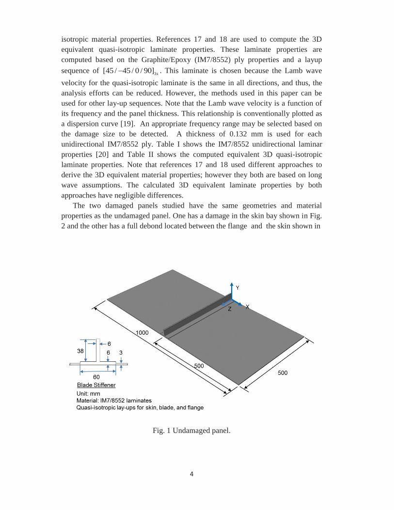
All panels studied in this paper, including undamaged and damaged ones shown in Figs 1 to 3, have the same geometries and material properties. All panels are assumed to have free boundary conditions along their edges. The dimensions of all panels are the same as shown in Fig. 1 for the undamaged panel. The panel contains two skin bays and one blade stiffener at the middle. The length and the width of this panel are 1000 mm and 500 mm, respectively. The flange width on each side of the blade is 27 mm wide (see the inset in Fig. 1). Both the skin and the flange have the same thickness of 3 mm and the blade has a thickness of 6 mm. Note that the origin of the coordinate system shown in Figs. 1 to 3 is located on the skin side at the right end of the blade stiffener, see Fig. 2. The Y and Z axes are in the midplane of the blade and Y=0 is at the skin-blade interface. The skin, blade and flange have quasi-

4

isotropic material properties. References 17 and 18 are used to compute the 3D equivalent quasi-isotropic laminate properties. These laminate properties are computed based on the Graphite/Epoxy (IM7/8552) ply properties and a layup sequence of 3[45 / 45 / 0 / 90] s . This laminate is chosen because the Lamb wave velocity for the quasi-isotropic laminate is the same in all directions, and thus, the analysis efforts can be reduced. However, the methods used in this paper can be used for other lay-up sequences. Note that the Lamb wave velocity is a function of its frequency and the panel thickness. This relationship is conventionally plotted as a dispersion curve [19]. An appropriate frequency range may be selected based on the damage size to be detected. A thickness of 0.132 mm is used for each unidirectional IM7/8552 ply. Table I shows the IM7/8552 unidirectional laminar properties [20] and Table II shows the computed equivalent 3D quasi-isotropic laminate properties. Note that references 17 and 18 used different approaches to derive the 3D equivalent material properties; however they both are based on long wave assumptions. The calculated 3D equivalent laminate properties by both approaches have negligible differences.

The two damaged panels studied have the same geometries and material properties as the undamaged panel. One has a damage in the skin bay shown in Fig. 2 and the other has a full debond located between the flange and the skin shown in

Fig. 1 Undamaged panel.

5

TABLE I. UNIDIRECTIONAL GRAPHITE/EPOXY (IM7/8552) PLY MATERIAL PROPERTIES.

Properties Reference 19 1E 161.34 GPa 2E 11.38 GPa 3E 11.38 GPa

23 0.45 13 0.32 12 0.32 23G 3.93 GPa 13G 5.17 GPa 12G 5.17 GPa

TABLE II. 3D EQUIVALENT LAMINATE PROPERTIES. Properties References 17&18

Ex 61.758 GPa Ey 61.758 GPa Ez 13.608 GPa

yz 0.3161 xz 0.3161 xy 0.3188

Gyz 4.466 GPa Gxz 4.466 GPa Gxy 23.415 GPa

Density 1.622x10-9 tonne/mm3

Fig. 3. The skin-bay damaged panel shown in Fig. 2 has a rectangular shaped damage of 30.30 mm x 3.13 mm that is centered at X=-305.73 mm and Z=250.00 mm. The panel with a full debond between the flange and the skin is shown in Fig. 3. The full debond region covers X=-30 mm to 30 mm and Z= 204.55 mm to 234.85 mm.

All panels are modeled with very fine meshes of 3D elements, C3D8R. Note that reference 9 also uses this ABAQUS element for modeling a composite panel. The dimensions of an element are approximately 1.5mm x 1.5mm x 1.5mm and there are two elements in the thickness direction. The same finite element mesh is used for both the undamaged and damaged panels; each finite element model contains 705,507 nodes and 481,818 elements. The ABAQUS/Explicit analyses are

6

performed with a very small time step, 85.0 10 secdt x , to assure that the Courant–Friedrichs–Lewy condition (CFL condition) is met for maintaining the accuracy of solutions [21].

In this study, no experimental tests were conducted and no real actuators were used to generate Lamb waves and no real sensors were used to receive the scattered wave signals. In finite element model, a node that mimics an actuator location is called an actuator node and a node that mimics a sensor location is called a sensor node. Note that that term ‘sensor node array” means a group of sensor nodes located in a line. The finite element model of the skin-bay damaged panel has a sensor node array that consists of nine sensor nodes (#1 to #9), shown in the inset close-up view of the sensor nodes in Fig. 2, These sensor nodes are used for receiving the scattered wave signals from the skin-bay damage. Note the sensor node #7 is inside the actuator location, see the bottom inset in Fig. 2. The sensor-node array is located at x=-150.63 mm and is distributed from Z=180.30 mm to 275.76 mm. The coordinates of sensor nodes (#1 to #9) are shown in Table III. The finite element model of the debond panel has a sensor node array that consists of six sensor nodes (#10 to #15), see the inset close-up view of the sensor nodes in Fig. 3. The sensor-node array is located at x=150.63 mm and evenly distributed from Z=163.64 mm to 224.24 mm. The coordinates of sensor nodes (#10 to #15) are shown in Table III. For the finite element model of the undamaged panel, it is assumed that the panel contains both sensor-node arrays at the same locations as shown in Figs. 2 and 3. The wave signal received at a sensor node is the baseline wave signal to be used in Section 4 for computing the scattered wave signal, wave signal reflected from the damage.

All wave signals are numerically obtained based on the results from ABAQUS/Explicit finite element analyses of the undamaged and damaged panels. In the finite element analysis, a flexural Lamb wave (antisymmetric mode) is generated by simultaneously applying a tone burst as a Y-displacement to every node in an actuator location. The detailed description of the tone burst is given in the next section. The actuator location that contains 12 actuator nodes located on a circle of diameter 6.16 mm is shown in the inset in Fig. 2. The actuator location for the undamaged and damaged panels are the same, centered at X=-150.63 mm and Z=250.00 mm, as shown in Figs. 2 and 3.

7

Fig. 2 Panel with a skin-bay damage.

TABLE III COORDINATES OF SENSOR NODES Sensor nodes X (mm) Y (mm) Z (mm)

1 -150.63 3 180.30 2 -150.63 3 192.42 3 -150.63 3 204.55 4 -150.63 3 216.67 5 -150.63 3 228.79 6 -150.63 3 240.91 7 -150.29* 3 250.62 8 -150.63 3 263.64 9 -150.63 3 275.76 10 150.63 3 163.64 11 150.63 3 175.76 12 150.63 3 187.88 13 150.63 3 200.00 14 150.63 3 212.12 15 150.63 3 224.24

*minor coordinate shift expected not affecting the results.

8

Fig. 3 Panel with a skin-stiffener debond.

3. GENERATION OF A 50 kHz TONE BURST

The tone burst used in this study is shown in Fig. 4 which has 3.5 cycles with a center frequency of 0.05 MHz (50 kHz). This tone burst is generated by modulating a sine wave function with a Hanning window [22] to warrant a narrow banded frequency spectrum for minimizing the dispersive nature of the Lamb wave. The equation used for generating the tone burst is:

2( ) sin(2 ) (1 cos( )), 0 12 3.50, 0 1

cc

f tAy t f t for t t

for t (1)

where y(t) is the signal amplitude at time t, A=0.05 mm is the maximum amplitude, 0.05cf MHz is the central frequency of the tone burst, and 1 70t s is the total

signal time. The FFT spectrum of the tone burst is plotted in Fig. 5. It clearly shows that the tone burst is narrowly banded and has a central frequency of 0.05 MHz.

9

0

0.2

0.4

0.6

0.8

1

0 0.05 0.1 0.15 0.2

Nor

mal

ized

Am

plitu

de

Frequency (MHz)

Fig. 4 3.5 cycle tone burst.

Fig. 5 FFT spectrum of the tone burst.

10

4. BAY DAMAGE LOCATION AND SIZE IDENTIFICATION

To simulate the use of Lamb waves for detecting damage in the skin bay of a stiffened panel, the damaged panel shown in Fig. 2 is analyzed. In this case study, the skin-bay damage shown in Fig. 2 is assumed to be a severe damaged region represented by a 90% reduction in the material properties. All the properties listed in Table 2 except the Poisson’s ratios and density are reduced. Note that representing damage in a composite laminate by reducing its material properties has been commonly used in composite progressive failure analyses [23]. By applying the tone burst shown in Fig. 4 to the 12 actuator nodes at the actuator location (shown in Fig. 2) as the Y-displacement (U2) input for each node, a propagating flexure Lamb wave (antisymmetric mode) is generated. The initial Lamb wave packet (group of waves) induced by the tone burst is shown in Fig. 6a. The Lamb waves propagate and interact with the stiffener and the skin-bay damage. Figure 6b clearly shows the scattered waves from the stiffener flange. The interaction with the damage generates scattered waves as shown in Fig. 6c. These scattered waves back propagate to the sensor nodes. Other scattered waves from the panel boundaries and

Fig. 6 Snapshots of propagating flexure Lamb wave in the skin-bay damaged panel.

11

the stiffener’s flange and blade need to be removed because they can mask the scattered wave from the damage. To remove the effects of these unwanted scattered waves, the damage induced scattered wave signal received at a sensor node need to be obtained by subtracting the wave signal of the undamaged panel ( baselinew ) from

the wave signal of the damage panel ( damaged panelw ) ,

( ) ( ) ( )scattered wave damaged panel baselinew t w t w t (2)

Scattered wave signals thus synthesized are based on the ABAQUS/Explicit FE analysis results of the damaged and the undamaged panels. In real structural health monitoring, these scattered wave signals will be experimentally obtained. The scattered wave signals received by all sensor nodes are then time reversed as shown in Fig. 7. These time-reversed scattered wave signals are re-emitted from their corresponding sensor node locations to generate back propagating waves for damage detection. The back propagating waves thus generated are called the “time reversal waves”. The time reversal waves from the sensor nodes are gradually

Fig. 7 Time-reversed scattered wave signals to be re-emitted from sensors #1 to #9.

s

12

converging to form a wave packet that propagates toward the damage location as shown in Fig. 8a to 8c. Note that the U2 displacement legend in these figures represents the Y-displacement. In this paper, a group of time reversal waves is called a wave packet. In the time reversal wave propagation simulation, the

a) Wave field formed by time-reversed sensor signals at t=94.05 s

b) Wave field formed by time-reversed sensor signals at t=126 s

Fig. 8 Propagation of the time reversal waves from the sensor nodes for skin bay damage detection.

13

c) Wave field formed by time-reversed sensor signals at t=152 s

Fig. 8 Propagation of the time reversal waves from the sensor nodes for skin bay

damage detection (Continued).

ABAQUS/Explicit analysis is performed with the finite element model of the undamaged panel. Note that in the actual structural health monitoring application, the damage location and size are unknown. The time reversal waves from the sensor nodes can be used to identify the damage location and to generate the damage image for estimating the damage size. Approaches 1 and 2 below present how to identify the damage location by using time of flight (TOF) and damage locus [8], the envelop of potential damage locations. The final damage location is determined by finding the intersection between the path of the time reversal waves and the damage locus. The damage locus is formed by using Approach 2 below. The damaged area in the 2D plane of the skin bay can be imaged by using appropriate imaging conditions [14]. Approach 3 below presents how to generate the damage image. 1. Determine the locus of potential damage locations based on the TOF

To obtain the locus of potential damage locations, the TOF needs to be determined first. The TOF can be determined by the time lag between the tone burst and the wave signal received by the sensor node #7. To determine the time lag, the cross-correlation of the tone burst and the scattered wave signal received by a sensor node #7 is computed as shown in Figs. 9a to 9c. Note that the sensor node #7 is located inside the actuator location (see Fig. 2). The time lag between the tone burst, ( )tone burstw t , and the scattered wave signal, ( )scattered wavew t , received

by the sensor node can be determined by identifying the maximum cross-

14

correlation value as shown in Fig. 9c. Note that both ( )tone burstw t and

( )scattered wavew t are discrete time signals. The cross-correlation value at time t ,

CCV(t), shown in Fig.9c was computed using the following equation [24],

1

0( ) ( ) ( ), 0,1,2,...., 1

N k

tone burst scattered waven

CCV t w n k w n k N (3)

where N is the length of both wave signals and time t k tt ( tt is the sampling time interval). The TOF is half of the time lag, 182.50 s , shown in Fig. 9c. The estimated distance between the actuator location and damage is 152.39 mm that is determined by multiplying the group velocity by the TOF [8]. This group velocity is 1.67 /mm s , computed theoretically [19] based on the 3D equivalent properties listed in Table II. Note that the group velocity predicted by the finite element model is within 1% of the theoretical value, indicating that the finite element model is adequate for the simulation of Lamb wave propagation. Using that distance as the radius and the actuator location as the center, a locus of likely damage locations can be determined, see Fig. 10.

a) Tone burst

b) Scattered wave signal received at sensor #7

Fig. 9 Determination of time lag between the tone burst and the scattered wave signal received by sensor node #7.

15

c) Time lag determined by time to the maximum cross-correlation value

Fig. 9 Determination of time lag between the tone burst and the scattered wave signal received by sensor node #7 (Continued).

Fig.10 Determination of damage location using the intersection point of the

damage locus and the path of the time reversal wave packet.

2. Estimate the intersection point between the damage locus and the path of the time reversal wave packet The time reversal wave packet is formed by the re-emitted time-reversed scattered wave signals from the nine sensor nodes. As illustrated in Fig. 10, the time reversal wave packet from sensor node array is propagating toward the damage location. The point where the wave packet crosses the damage locus is

16

the damage location. This approach for finding the damage location is based on the Huygens’ Principle [4]: every point on a wave front can be considered as a secondary source of spherical waves. Thus, the recorded wave field is back propagated, at a certain time the wave front will be coincident with the reflector or the secondary source. In other words, the time reversal waves from a sensor-node array will converge at the damage locations.

3. Image the damage By applying an image condition [14] to the FE nodes in the neighborhood of the damage location, a damage image can be created. The image condition used in this paper is the zero-lag cross-correlation value (ZLCCV) at a finite element node. Note that for an infinitesimal damage size, the time-reversed incident wave signal, * ( )incident wavew t , and the signal from the time reversal wave packet,

* ( )wave from sensor nodesw t , will theoretically propagate to the damage location

(reflector) at the same time [4]. Note the superscript * indicates that the time reversal method is used to obtain the wave signal. For a finite size damage, it is expected that these two signals arrive at a node in the damage region near the same time. Thus, the ZLCCV of these two functions has a greater value at a node in the neighborhood of the damage location than at a node away from the damage. The ZLCCV is computed at a node i in the neighborhood of the damage location, using the following equation,

1

* *

0( ) ( )

N

i incident wave wave from sensor nodesn

ZLCCV w n w n (4)

where N is the length of both wave signals. A contour of ZLCCV=0.0 in the neighborhood of the damage location can be identified as shown in Fig. 11. The region inside the contour of the zero ZLCCV contour is the damage image, greater ZLCCV indicting more severe damage. The damage image thus generated is shown in Fig 11. The damage image is overlaid on the original rectangular shaped damage for evaluating the quality of the damage image. It is found that the damage location and the damage size are reasonably well captured. An offset of the damage image about 3mm to the right of the actual rectangular location may be because most of the scattered waves that the sensor nodes received are reflected from the front edge of the rectangular damage zone. Since the material properties in the damage zone are reduced by

17

Fig. 11 Damage image correlating with actual damage area (Right legend

shows ZLCCVs)

90%, it is expected that much weaker waves could be reflected from other edges. Multiple sensor-node arrays located at various locations and multiple actuators in each sensor-node array are needed for better determining damage location and size.

Using the aforementioned approaches, the damage location and the image of damage for estimating damage size can be obtained. This damage imaging process is computationally efficient since only the ZLCC values of a small amount of nodes in the neighborhood of the identified damage location are computed instead of those of the full model.

5. DEBOND LOCATION AND SIZE IDENTIFICATION

A finite element model was created for the stiffened panel with an assumed skin and stiffener-flange debond shown in Fig. 3. Using double nodes in the debond region, the elements modeling the skin are fully separated from the stiffener and flange elements. The flexural Lamb waves, generated by applying the tone burst at the actuator location shown in Fig. 3, propagate into the debond region to reach the next skin bay as shown in Figs. 12a and 12b. Note that the waves that propagate through the debond region have a greater amplitude than those through the undebond regions as shown in Fig. 12b. Sensor-nodes in the next skin bay, shown in Fig. 3, will receive much stronger wave signals compared to the signals received

18

from the baseline signals of the undamaged panel. By subtracting the baseline signals from the stronger signals of the debond panel, differential wave signals due to the effect of the debond for each sensor node can be obtained. Since the differential wave signals only contain the effects of the debond damage, it is appropriate to consider the debond as a source. Thus, these differential wave signals received by the sensor nodes can be time reversed and re-emitted to generate back propagating waves for detecting the debond.

The time-reversed signals of the six sensor nodes (#10 to #15) are plotted in Fig. 13. ABAQUS/Explicit FE analysis was performed to simulate the propagation of these time-reversed differential signals and the results are shown in Fig. 14a to 14c. Note in the ABAQUS/Explicit FE analysis, the undamaged finite element model is used. These waves are converging to form two wave packets as shown in Fig. 14b since there is no restriction applied in the analysis model to limit the waves propagating in only one direction. One of the wave packets propagates toward the stiffener and meets the stiffener at the debond as clearly shown in Fig. 14c. The intersection point for the flange edge and the time reversal wave packet may be used to determine the debond location along the Z-axis (see Figs. 3 and 14c) and the amplitude of the time reversal wave packet may be used to estimate the debond width in the Z-direction.

a) Wave field at t=75 s

Fig. 12 Snapshots of propagating flexure Lamb wave in the debond panel.

19

b) Waves field at t=175 s

Fig. 12 Snapshots of propagating flexure Lamb wave in the debond panel (Continued).

Fig. 13 Time-reversed wave signals of sensor nodes #10 to #15 in the debond panel model.

20

a) Time reversal wave packet at t=100 s

b) Time reversal wave packet at t=110 s

Fig. 14 Propagation of time reversal differential waves for debond detection.

21

c) Time reversal wave packet at t=140 s

Fig. 14 Propagation of time reversal differential waves for debond detection (Continued).

6. CONCLUDING REMARKS

This study simulates the detection of damage in composite stiffened panels using Lamb waves. This virtual test process based on the ABAQUS/Explicit FE analysis results does not need to use real structures, actuators/sensors, or laboratory equipment. The methodologies used in this paper can be equally applied to experimentally obtained Lamb waves. The detection of two types of damage is studied. One type is a damage in the skin bay. The other type is a debond between the stiffener flange and skin. The methods used in this research include: 1) the propagation of the time-reversed scattered or differential waves from the sensor nodes, and 2) the use of signal processing techniques to image the damage. Results show that the damage location and the damage size may be identified using the current approaches. Note that only one actuator location and one sensor-node array are used for studying a single damage in the panel. Future studies may include aircraft structures with multiple damages and use more sensor-node arrays and multiple actuator locations in each sensor-node array to be able to more accurately identify the damage location and more precisely determine the damage size.

REFERENCES

1. Lin, X. and F.G. Yuan, “Diagnostic Lamb waves in an integrated piezoelectric sensor/actuator plate: analytical and experimental studies,” Smart Materials & Structures, Vol. 10, pp. 907-913, 2001.

22

2. Wang, C.H., J.T. Rose, and F.K. Chang, “A synthetic time-reversal imaging method for structural health monitoring,” Smart Materials & Structures, Vol. 13, pp. 415-423, 2004.

3. Rose, J.L., “Ultrasonic guided waves in structural monitoring,” Key Engineering Materials, Vols. 270-273, pp. 14-21, 2004.

4. Lin, X. and F.G. Yuan, “Damage detection of a plate using migration technique,” Journal of Intelligent Material Systems and Structures, Vol. 12, pp. 469-482, 2001.

5. Raghavan, A. and C.E.S. Cesnik, “Finite-dimensional piezoelectric transducer modeling for guided wave based structural health monitoring,” Smart Materials & Structures, Vol. 14, pp. 1448-1461, 2005.

6. Park, H.W., H. Sohn, K.H. Law, and C.R. Farrar, “Time reversal active sensing for health monitoring of a composite plate,” Journal of Sound Vibration, Vol. 302, pp. 50-66, 2007.

7. Gangadharan, R., C.R.L. Murthy, S. Gopalakrishnan, and M.R. Bhat, “Time reversal technique for health monitoring of metallic structure using Lamb waves,” Ultrasonics, Vol. 49, pp. 696-705, 2009.

8. Lin, X. and F.G. Yuan, “Experimental study applying a migration technique in structural health monitoring,” Structural health Monitoring, Vol. 4, No. 4, pp. 341-353, 2005.

9. NG, C.T. and M. Veidt, “A Lamb-wave-based technique for damage detection in composite laminates,” Smart Materials & Structures, Vol. 18, pp. 1-12, 2009.

10. Leckey, C.A.C., M.D. Rogge, C.A. Miller, and M.K. Hinders, “Multiple-mode Lamb wave scattering simulations using 3D elastodynamic finite integration technique,” Ultrasonics, Vol. 52, pp. 193-207, 2012.

11. Yu, L. and C.A.C. Leckey, “Lamb wave based quantitative crack detection using a focusing array algorithm,” Journal of Intelligent Material Systems and Structures, 2012, doi:10.1177/1045389X12469452 .

12. Rogge, M.D. and C.A.C. Leckey, “Characterization of impact damage in composite laminates using guided wavefield imaging and local wavenumber domain analysis,” Ultrasonics, 2013, http://dx.doi.org/10.1016/j.ultras.2012.12.015.

13. Song, F., G.L. Huang, and G.K. Hu, “Online guided wave-based debonding detection in honeycomb sandwich structures,” AIAA Journal, Vol. 30, No. 2, pp. 284-293, 2012.

14. Chattopadhyay, S. and G.A. McMechan, “Imaging conditions for prestack reverse-time migration,” Geophysics, Vol. 73, No. 3, pp. S81-S89, 2008.

15. Giurgiutiu, V., L. Yu, J.R. Kendall III, and C. Jenkins, “In situ Imaging of crack growth with piezoelectric-wafer active sensors,” AIAA Journal, Vol. 43, No. 11, pp. 2758-2769, 2007.

16. ABAQUS Analysis User’s Manual, Version 6.11, ABAQUS Inc., 2011. 17. Sun, C.T. and S. Li, “Three-dimensional effective elastic constants for thick laminates,” Journal

of Composite Materials, Vol. 22, pp. 629-639, 1988. 18. Akkerman, R., “On the properties of quasi-isotropic laminates,” Composites, Part B, Vol. 33,

pp. 133-140, 2002. 19. Wang, L., Elastic wave propagation in composites and least-squares damage localization

technique, Master of Science thesis, Aerospace Engineering of North Carolina State University, 2004.

20. Roh, H.S., and C.T. Sun, “The Strength of Double Strap Joint with Brittle and Ductile Adhesives,” in Volume 4: Failure in Composites (Fourth volume in the American Society for Composites' Series on Advances in Composite Materials), Edited by: Anthony M. Waas and Bhavani V. Sankar, December, 2012.

21. Courant, R., K. Friedrichs, and H. Lewy, "Über die partiellen Differenzengleichungen der mathematischen Physik," Mathematische Annalen, Vol. 100, pp. 32–74, 1928.

22. Wikipedia, “Window function”, http://en.wikipedia.org/wiki/Window_function 23. Knight, N.F., User-defined material model for progressive failure analysis, NASA/CR-2006-

214526, December, 2006.

23

24. MathWorks R2013a Documentation, http://www.mathworks.com/help/signal/ref/hann.html