Simulation of Damage for Wind Turbine Blades Due to...

Simulation of Damage for Wind Turbine Blades Dueto Airborne Particles

Giovanni Fiore1 and Michael S. Selig2*

1Ph.D. Candidate, Department of Aerospace Engineering, University of Illinois at Urbana-Champaign, Urbana, Illinois 61801, USA, Email: [email protected] Professor, Department of Aerospace Engineering, University of Illinois at Urbana-Champaign, Urbana, Illinois 61801, USA, Email: [email protected]

ABSTRACTA mathematical model and simulation of airborne particle collisions with a 38 m, 1.5 MW horizontal axis wind turbine bladeare presented. Two types of particles were analyzed, namely insects and sand grains. Computations were performed using atwo-dimensional inviscid flowfield solver coupled with a particle position code. Three locations along the blade were consideredand characterized by airfoils of the DU series. The insect simulations estimated the residual debris thickness on the blade,while sand simulations computed the surface erosion rate. Results show that the impact locations along the blade depend onangle of attack, freestream velocity, airfoil shape, and particle mass. Particles were found to collide primarily at the leadingedge. The volume of insect debris per unit span was maximum at r /R = 0.75. The erosion rate due to sand was maximumon the low pressure side of the blade. An erosion rate approximately ten times higher was observed at r /R = 0.75, ascompared with the section at r /R = 0.35. Near the leading edge, large angles of impact occurred and erosion rate had aminimum, while it reached maximum values slightly downstream where the impact angle was more skewed.

Received 12/01/2014; Revised 02/25/2015; Accepted 02/25/2015

NOMENCLATURE

WIND ENGINEERING Volume 39, No. 4, 2015 PP 399–418 399

*Corresponding Author: E-mail address: [email protected].

A = particle reference areaAK = particle nondimensional massc = airfoil chord lengthCOE = Cost of EnergyCd = airfoil drag coefficientCD = particle drag coefficientCl = airfoil lift coefficientd = particle diameterD = particle drag forceE = erosion rateEI = particle impact efficiencyER = insect rupture efficiencyf = sand grain shape factorGAEP = Gross Annual Energy Productionh = airfoil projected height

perpendicular to freestreamK = erosion rate constantl = particle lengthm = particle massn = erosion rate velocity exponentQ = quantity of insect debris

r/R = airfoil radial location on bladeRI = impact surface ratioRR = rupture surface ratioRe = particle Reynolds numberRe∞ = freestream Reynolds numbers = impact location along airfoil arc

lengthstot = airfoil total arc lengtht = timet/c = airfoil thickness-to-chord ratioU = chordwise velocity componentV = chord-normal velocity

componentV∞ = freestream velocityVimp = particle impact velocityVN = particle normal impact velocityVr = particle relative velocityVrup = insect rupture velocityx = particle x-locationy = particle y-locationα = angle of attack

αr = relative angle between theflowfield and particle velocity

β = impingement efficiencyε = excrescence heightηR = insect rupture ratioλ = tip-speed ratioθ = impact angleμ = dynamic viscosityρ = densityτ = nondimensional time

Subscripts and superscripts0 = initial statel = lower limitI = insectP = particler = relativeS = sandu = upper limit

400 Simulation of Damage for Wind Turbine Blades Due to Airborne Particles

1. INTRODUCTIONHorizontal axis wind turbines (HAWTs) used for eletrical power generation are subject to foulingand damage by airborne particles associated with the environment in which wind turbines operate.Throughout the 20-year lifespan of a wind turbine, particles such as raindrops, sand grains, icecrystals, hailstones, and insects are major contributors to a deterioration in turbine performancethrough local airfoil surface alterations [1–4]. Turbine blades accumulate dirt especially in thesurroundings of the leading edge. Moreover, particle collisions, temperature jumps and freeze-thawcycles may cause existing cracks in the coating to propagate, promoting coating erosion, coredelamination, and corrosion damage due to exposure of the internal composite structure. Theoriginally smooth surface of the blades may change considerably, and in such cases the increasedroughness will cause a reduction in power output. For instance, once an insect collides and adheresto the surface of the blade, the boundary layer is adversely affected and local flow separation mayoccur if the residual debris thickness is comparable to the boundary layer critical height [5, 6].However, even when this situation is seemingly minor, the drag coefficient is still increased due toboundary layer early transition [7]. When substantial insect fouling occurs, the critical roughnessheight is easily reached in the proximity of the blade leading edge. In such conditions, a bimodalelectrical power output behavior was observed for stall-regulated HAWTs [8]. Reductions of thenominal power output up to 25% were reported during high wind days for this type of turbine [9].

New advancements in wind resource assessment have shown the benefits of offshore megawatt-scale wind turbine installations [10, 11], in order to maximize GAEP while reducing COE. However,offshore locations are subject to more intense sand erosion than the majority of land installations[12–14]. Airborne sand particles collide with the blade and cause microcutting and plowing in thecoating material [15, 16] resulting in surface abrasion [17, 18]. Such damage is particularlyprominent at the outboard sections of the blade where the local relative velocity is larger comparedwith inboard sections [12].

Wind farm operators are forced to schedule blade inspection and maintenance to reduce the costof ineffective electric power production due to degraded wind turbine blades. Disassembling awind turbine for factory inspection is costly, so the majority of servicing is performed on site.Damaged areas are located through blade visual inspection, surface alterations are smoothedthrough primer application and a protective polyurethane-based film is applied [19, 20]. However,because of the highly competitive nature of the wind turbine industry, the majority of wind turbinemanufacturers are reluctant to share details of the construction materials with maintenancecompanies. Therefore, technical expertise plays a critical role in blade repair success andeffectiveness [2, 21]. Moreover, repairs are mostly performed in the vicinity of the leading edgeand not necessarily on all areas exposed to damage. Further downstream, blade areas eroded bysand and damaged by insect debris may be left untreated, promoting the enlargement of surfacedamage starting at coating weakened points. An estimated 6% of overall repairs and maintenanceresources for wind turbines is dedicated to rotor blades [22, 23]. Moreover, an analysis of windturbine reliability showed that tip break and blade damage are the first and third most commonfailure modes for wind turbines, respectively [23].

A few other detrimental aspects are involved with wind turbine operational damage. From anaerodynamic standpoint, a reduction in aerodynamic efficiency associated with an increase of thedrag coefficient results from exposure to environmental airborne particles [24–26]. Also, an increasingly important issue associated with damaged blades is the level of noise generated. Bladesurface alterations may increase the level of noise generated by perturbing the boundary layer

pattern [27]. From a technological stand-point, specialized surface coatings have been developed toassure a consistent aerodynamic performance and adequate structural integrity throughout thelifespan of a wind turbine [28]. Modern wind turbines are delivered with a factory-applied coating,and the majority of coating materials are polyurethane-based [29].

The goal of this study was to compute the trajectory of insects and sand grains and tocharacterize the impact areas of three sections along a wind turbine blade located at 35%, 65% and75% of the span. A three-blade, 38 m radius, 1.5 MW HAWT was chosen as a baseline for thecomputations, being at present the most common wind turbine configuration in North America [30].Two computational models were implemented to characterize the damage due to insect fouling andsand erosion, and these models are discussed. This paper is divided into five sections: the numericalmethod used for the computations is described in Section 2, the blade operating point, particleaerodynamics, and blade damage models are introduced in Section 3, the results obtained alongwith a proposed operational damage model are discussed in Section 4, and finally, conclusions arepresented in Section 5.

2. METHODOLOGY AND THEORETICAL DEVELOPMENTPredicting the trajectory of impinging particles is critical when impact characteristics on the windturbine blade need to be determined. A lagrangian formulation code was developed in-house andnamed BugFoil. BugFoil integrates a pre-existing insect trajectory code [31] and a customizedversion of XFOIL [32]. Local flowfield velocity components are obtained by querying the potentialflow routine built in XFOIL, from which the particle trajectory and impact location on the airfoilare computed. Similarly, the capabilities of BugFoil have been expanded to simulate trajectories ofsand grains.

In steady flight, the forces acting on the particle are perfectly balanced. Perturbations to suchforces are assumed to be additive to the steady-state forces. For these reasons the equations ofmotion may be expressed by neglecting the steady-state forces and may be written as functions ofincrements only [33]. In the current study, both insects and sand grains were treated as aerodynamicbodies whose only associated force is the aerodynamic drag D. The main advantage of thisassumption was to simplify the evaluation of insect trajectory because the effects of lift due to thewings are considered to be negligible compared with drag and inertia forces. It should be noted herethat regardless of the insect and blade relative orientation during impact, the chosen approachallowed for trajectory evaluation. On the other hand, considering the insect lift force would pose theissue of estimating the direction and magnitude of such force in a two-dimensional plane throughoutthe entire rotating envelope of the wind turbine blade.

By applying Newton’s second law along the particle trajectory in both chordwise x and chord-normal y directions, the following equations are obtained [15, 34–36]

(1)

(2)

By projecting the drag of the particle D in both chordwise x and chord-normal y directions usingthe relative angle between particle and flowfield velocity αr, the equations may be rewritten as

(3)

(4)

Given the particle velocity components UP and VP and given the velocity flowfield componentsU and V at a certain point along the trajectory, the relative particle velocity Vr can be expressed as

(5)

while the trigonometric functions in Eqs. (3) and (4) may assume the form

=∑md x

dtFp

px

2

2

=∑md y

dtFp

py

2

2

α= Δmd x

dtD cosp

pr

2

2

α= Δmd y

dtD sinp

pr

2

2

= − + −V U U V V( ) ( )r p p2 2

WIND ENGINEERING Volume 39, No. 4, 2015 401

(6)

(7)

By expressing the particle aerodynamic drag D as a function of dynamic pressure and bysubstituting for the trigonometric functions, Eqs. (3) and (4) may be rewritten as

(8)

(9)

To scale this problem in a non-dimensional fashion, non-dimensional time, space, and massparameters can be introduced as

(10)

(11)

(12)

(13)

Nondimensionalization of Eqs. (8) and (9) by the reference velocity U yields

(14)

(15)

which represents a set of second-order, nonlinear differential equations. Once the drag coefficient of theparticle is evaluated, the trajectory can be computed by numerically solving both x and y equations.

3. BLADE DAMAGE ANALYSISThe selected configuration is a three-blade, 1.5 MW, 38 m radius, λ = 8.7 wind turbine. Starting atthe blade root and moving toward the tip, the airfoils used are the DU 97-W-300, DU 96-W-212,and DU 96-W-180. The airfoils relative thickness t/c and chord length c decrease along the bladespan, in accordance to conventional wind turbine designs. A wind speed of 10.5 m/s at the hubheight was selected for the chosen configuration [37]. The blade properties and inflow conditionsare summarized in Table 1. Since modern wind turbines are operated close to their maximum lift-to-drag ratio [37, 38], the three sections of the blade were analyzed with XFOIL and three valuesof Cl were determined in the proximity of (Cl /Cd)max. The operating conditions for the three bladesections are given in Table 2. Simulations for impact and damage due to insects and sand grainswere performed at three angles of attack corresponding to the values of Cl determined.

3.1. Trajectory evaluationBugFoil is initialized using nondimensional input data. An equally-spaced array of particles isplaced five chord lengths upstream of the airfoil, with both initial velocity componentsnondimensionalized with respect to the local freestream velocity V∞. Each particle is evaluatedindividually throughout its trajectory by numerically solving the particle equations of motion

α =−

=U U

V

V

Vcos r

p

r

rx

r

α =−

=V V

V

V

Vsin r

p

r

ry

r

ρ=md x

dtV A C

V

V

1

2pp

r p Drx

r

2

22

ρ=md y

dtV A C

V

V

1

2pp

r p Dry

r

2

22

τ =tU

c

=xx

cpp

=yy

cpp

ρ=AK

m

A c

2 p

p

τ=

d x

d AKV C V

1pr D rx

2

2

τ=

d y

d AKV C V

1pr D ry

2

2


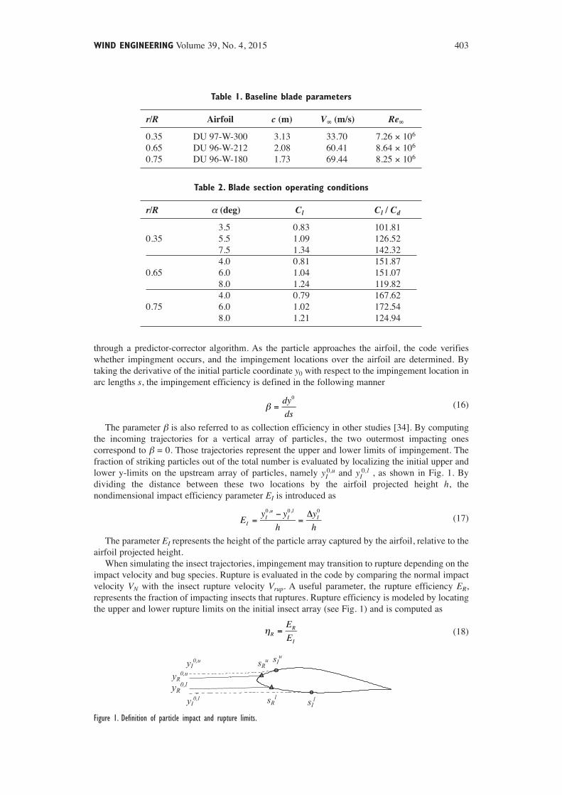
through a predictor-corrector algorithm. As the particle approaches the airfoil, the code verifieswhether impingment occurs, and the impingement locations over the airfoil are determined. Bytaking the derivative of the initial particle coordinate y0 with respect to the impingement location inarc lengths s, the impingement efficiency is defined in the following manner

(16)

The parameter β is also referred to as collection efficiency in other studies [34]. By computingthe incoming trajectories for a vertical array of particles, the two outermost impacting onescorrespond to β = 0. Those trajectories represent the upper and lower limits of impingement. Thefraction of striking particles out of the total number is evaluated by localizing the initial upper andlower y-limits on the upstream array of particles, namely yI

0,u and yI0,l , as shown in Fig. 1. By

dividing the distance between these two locations by the airfoil projected height h, thenondimensional impact efficiency parameter EI is introduced as

(17)

The parameter EI represents the height of the particle array captured by the airfoil, relative to theairfoil projected height.

When simulating the insect trajectories, impingement may transition to rupture depending on theimpact velocity and bug species. Rupture is evaluated in the code by comparing the normal impactvelocity VN with the insect rupture velocity Vrup. A useful parameter, the rupture efficiency ER,represents the fraction of impacting insects that ruptures. Rupture efficiency is modeled by locatingthe upper and lower rupture limits on the initial insect array (see Fig. 1) and is computed as

(18)

β =dy

ds

0

=−

=Δ

Ey y

h

y

hII

uI

lI

0, 0, 0

η =E

ERR

I


Table 1. Baseline blade parameters

r/R Airfoil c (m) V∞ (m/s) Re∞

0.35 DU 97-W-300 3.13 33.70 7.26 × 106

0.65 DU 96-W-212 2.08 60.41 8.64 × 106

0.75 DU 96-W-180 1.73 69.44 8.25 × 106

Table 2. Blade section operating conditions

r/R α (deg) Cl Cl / Cd

3.5 0.83 101.810.35 5.5 1.09 126.52

7.5 1.34 142.324.0 0.81 151.87

0.65 6.0 1.04 151.078.0 1.24 119.824.0 0.79 167.62

0.75 6.0 1.02 172.548.0 1.21 124.94

yI0,u

yI0,l

yR0,uyR0,l

sRu sIu

sRl sIl

Figure 1. Definition of particle impact and rupture limits.

A measure of the relative quantity of rupturing insects with respect to the impacting total is givenηR defined as follows

(19)

The parameter ηR represents a figure of merit of the airfoil since it incorporates the rupturingmechanism of insects. An advantage of using ηR is being independent from the airfoil projectedheight h, which may not have a linear relationship with the angle of attack.

One way to estimate the blade surface area subject to particle collisions is to compute the airfoilarc length within the upper and lower surface impingement limits, sI

u and sIl, respectively, as shown

in Fig. 1. The result of this operation is called ΔsI . By knowing the total airfoil arc length stot, theimpact surface ratio RI can be computed as

(20)

As RI approaches unity, a larger portion of the blade area is subject to particle collision. In a similarmanner, when considering the fouling due to insects, the rupture surface ratio RR may be defined as

(21)

The parameter RR represents the amount of blade surface where rupture occurs.

3.2. Aerodynamics of the insectEarly studies on atmospheric insect population were performed to sample and identify flying insectspecies in the atmospheric region 100 m above the ground in southern Great Britain [39]. It wasdiscovered that the most prominent species in those conditions were aphids and drosophilamelanogaster, commonly known as the fruit fly. At present, however, entomology literature doesnot report extensive studies on insect population around the world and at various aerial heights.Later aerodynamic studies conducted on fruit flies were able to estimate lift and drag coefficientsof the wings of such insects [40, 41] along with insect rupture velocity (Vrup = 10.8 m/s). Suchinformation was used to simulate drosophila head-on impingement over wings of air-planes [31].In the current study, however, the insect was considered to be steady in hovering flight, due to thelarge difference between the drosophila flying speed (≈ 2 m/s [42]) and the much higher blade localspeed (see Table 1). Moreover, the lift contribution due to the wings was considered negligible whencompared with inertia and drag forces of the body, as explained in Section 2.

The overall drosophila aerodynamic drag is dominated by viscous forces since its flightReynolds number is typically Re ≈ 102 [43–45]. The insect body drag coefficient can be approximatedby the drag coefficient of spherical shapes in the same Reynolds number range [35, 46] and byfitting it to experimental drag values for drosophila [31, 40], that is

(22)

where Re is based on insect body diameter. The reference value of drosophila body mass [31] is mI = 8.7 × 10–4 g. The drosophila input data used for computing trajectories is summarized inTable 3. Note that Vrup is nondimensionalized by V∞ at each blade section.

η =E

ERR

I

=−

=Δ

Rs s

s

s

sIIu

Il

tot

I

tot

=−

=Δ

Rs s

s

s

sRRu

Rl

tot

R

tot

= + × + ×CRe

Re Re9.8

(1 1.97 0.1 2.60 0.0001 )D0.63 1.38


Table 3. Insect input parameters

r/R Re AKI lI/c Vrup/V∞

0.35 1562.7 0.283 2.152 × 10–4 0.3220.65 2800.5 0.426 3.241 × 10–4 0.1800.75 3219.2 0.514 3.900 × 10–4 0.156

3.3. Insect foulingAfter impacting, insects leave streaks of fluids and fragments on the surface of the blade. The debristhickness, called here excrescence height ε , is numerically evaluated on the blade sections.Excrescence height is computed through normal impact velocity VN as an interpolation ofexperimental impact data for drosophilas [5, 47]. The maximum excrescence height follows thenondimensional empirical law given by [31]

(23)

where lI is the insect body length (see Table 3). The normalized excrescence height ε /lI as a functionof β is given as

(24)

where the coefficients ci are obtained by fitting experimental debris height measurements.Integrating ε /lI along the insect impingement limits over the airfoil yields the quantity of insectdebris Q, that is

(25)

The nondimensional parameter Q represents the volume of insect debris per unit span ofthe blade.

3.4 Aerodynamics of the sand grainAirborne sand particles are mainly represented by silica-based grains. To incorporate shapeirregularities typical of sand grains, the aerodynamic drag is modeled by means of a shape factor fdefined as [46]

(26)

where a is the surface area of a sphere with the same volume of the sand grain, and AS is the actualsurface of the sand grain. Note that for perfectly spherical particles the shape factor is equal to unity.The drag coefficient for a sand grain is written in the form [46]

(27)

where the bi coefficients are functions of f , and Rer is the relative Reynolds number defined as

(28)

The aerodynamic drag force can be expressed as [14, 36]

(29)

The sand grain lift coefficient CL is assumed to be negligible.

3.5. Sand erosionSand erosion has been investigated for a variety of air-breathing engines in aerospace applications[18, 36, 48, 49]. Sand grain velocities in the compressor stages are in the same range of the windturbine erosion scenario. Erosion is responsible for an increase in blade surface roughness and adecrease in structural stiffness. The parameter erosion rate E, defined as the removed mass of the target

εβ β β

⎛

⎝⎜

⎞

⎠⎟ = + + + + β

lc c c c c exp

I0 1 2

23

34

(c )5

∫ ε=Ql

ds1

Is

s

Il

Iu

=fa

As

ε⎛

⎝⎜

⎞

⎠⎟ =

⎛

⎝⎜⎜

⎞

⎠⎟⎟ −

⎛

⎝⎜⎜

⎞

⎠⎟⎟+l

V

V

V

V0.088165 0.53289 1.3856

I

N

rup

N

rupmax

2

= + ++

CRe

Reb

b

Re

24(1 b )

1D

rrb

r

13

4

2

ρ

μ=

−Re

ds Us UR

μ=ρ

Dd

C Re18

24s

D r2


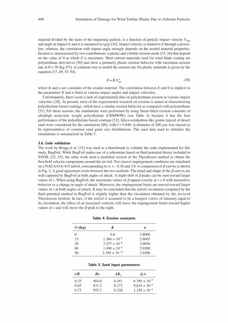
material divided by the mass of the impacting particle, is a function of particle impact velocity Vimp

and angle at impact θ, and it is measured in (g/g) [16]. Impact velocity is related to E through a power-law; whereas, the correlation with impact angle strongly depends on the eroded material properties.Erosion is characterized by two contributions: a plastic and a brittle erosion mode [15, 16] that dependon the value of θ at which E is maximum. Most current materials used for wind blade coating arepolyurethane derivatives [50] and show a primarily plastic erosion behavior with maximum erosionrate at θ = 30 deg [51]. A common way to model the erosion rate for plastic materials is given by theequation [17, 49, 52–54]

(30)

where K and n are constants of the eroded material. The correlation between E and θ is implicit inthe parameters K and n fitted at various impact angles and impact velocities.

Unfortunately, there exists a lack of experimental data on polyurethane erosion at various impactvelocities [28]. At present, most of the experimental research on erosion is aimed at characterizingpolyethylene-based coatings, which have a similar erosion behavior as compared with polyurethane[51]. For these reasons, the simulations were performed by using linear-fitted erosion constants ofultrahigh molecular weight polyethylene (UHMWPE) (see Table 4) because it has the bestperformance of the polyethylene-based coatings [52]. Silica octahedron-like grains typical of desertsand were considered for the simulation [46], with f = 0.846. A diameter of 200 μm was chosen tobe representative of common sand grain size distributions. The sand data used to initialize thesimulations is summarized in Table 5.

3.6. Code validationThe work by Bragg et al. [31] was used as a benchmark to validate the code implemented for thisstudy, BugFoil. While BugFoil makes use of a subroutine based on fluid potential theory included inXFOIL [32, 55], the other work used a modified version of the Theodorsen method to obtain theflowfield velocity components around the air-foil. Two insects impingement conditions are simulatedon a NACA 63A-415 airfoil, corresponding to α = – 0.36 and 3.0. A comparison of β-curves is shownin Fig. 2. A good agreement exists between the two methods. The trend and shape of the β-curves arewell captured by BugFoil at both angles of attack. A slight shift of β peaks can be seen toward largervalues of s. When using BugFoil, the maximum values of β appear exactly at s = 0 with insensitivebehavior to a change in angle of attack. Moreover, the impingement limits are moved toward largervalues of s at both angles of attack. It may be concluded that the airfoil circulation computed by thefluid potential method in BugFoil is slightly higher than the circulation obtained by the inviscidTheodorsen method. In fact, if the airfoil is assumed to be a lumped vortex of intensity equal toits circulation, the effect of an increased vorticity will move the impingement limits toward highervalues of s and will move the β-peak to the right.

=E K Vimpn


Table 4. Erosion constants

θ (deg) K n

0 0.0 2.800015 1.366 × 10–9 2.806530 3.337 × 10–9 2.605660 1.490 × 10–9 2.650090 2.350 × 10–11 2.6500

Table 5. Sand input parameters

r/R Re AKs ds /c

0.35 464.0 0.181 6.389 × 10–5

0.65 831.5 0.272 9.624 × 10–5

0.75 955.7 0.328 1.158 × 10–4

4. RESULTS AND DISCUSSIONAll simulations were performed by initializing BugFoil with the input parameters for insect andsand grain reported in Tables 3 and 5 respectively. Each location along the blade span was analyzedat three operating points corresponding to three angles of attack as reported in Table 2. A singlesimulation required an average of 2 sec of computation time on an Intel Core i7 machine with 8 GB RAM running LinuxMint OS.

In order to characterize the particle impact locations along the airfoil, a useful measure is givenby the airfoil arc length s. The parameter s is defined as the length of the arc starting at the particleimpact location and ending at the air-foil leading edge, normalized by the airfoil chord c. Note thats is negative for impingement locations on the lower side of the airfoil, while it is positive on theupper side. Also, the leading edge of a finite-thickness airfoil is located at s ≡ 0, while the trailingedge corresponds to values of |s| ≥ 1. Results for impact of insect and sand grain are discussed inSections 4.1 and 4.2 respectively.

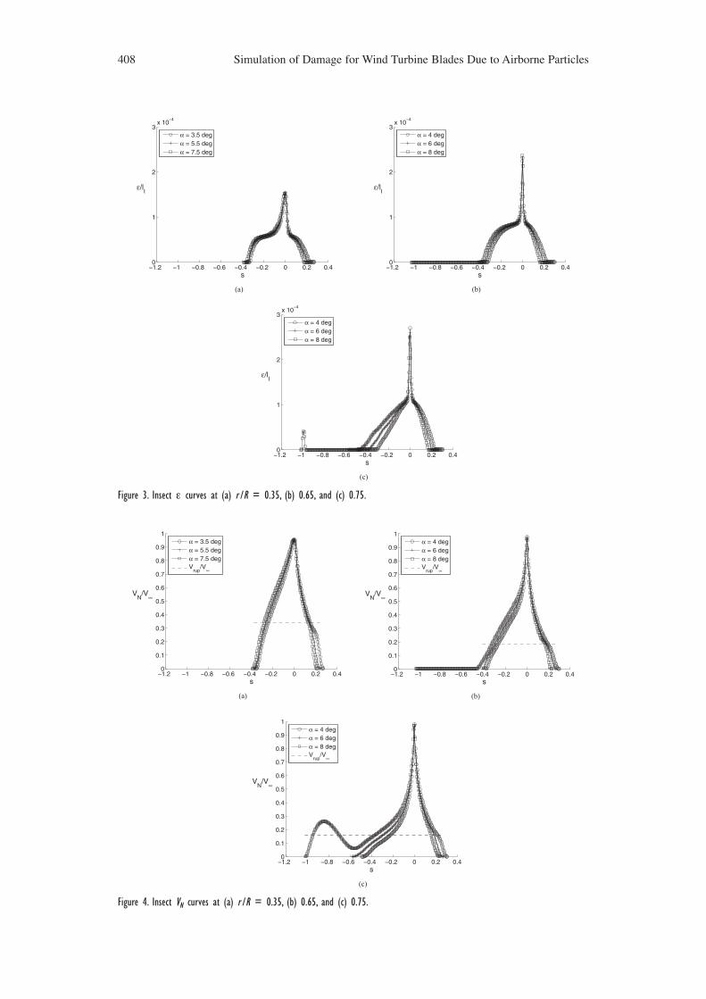
4.1. Insect simulationInsect trajectories and impact properties were evaluated at r/R = 0.35, 0.65 and 0.75, correspondingto the airfoils DU 97-W-300, DU 96-W-212, and DU 96-W-180, respectively. The normalizedexcrescence height ε with respect to insect length lI , and normalized normal impact velocity VN

with respect to V∞, are presented in Figs. 3, and 4, respectively, as a function of airfoil arc length s.Peak values of ε are reached in the vicinity of s = 0 at all sections. However, for the three casesconsidered the maximum value of ε is reached at r/R = 0.75, where the highest simulated freestreamvelocity occurs [Fig. 3(c)], while the peak of ε decays steadily when moving to inboard sections, asshown in Figs. 3(b) and 3(a). Changing angle of attack has a modest effect on the peak value ofexcrescence height. At increased angles of attack, maximum values of ε move slightly towardnegative values of s, following the shift in the stagnation streamline. Also, the insect impingementlimits move forward on the upper surface and aft on the lower surface with increasing angle ofattack. In fact, for α = 8 deg the lower impingement limit reaches the trailing edge of the airfoil, asshown in Figs. 3(c) and 4(c).

Normal impact velocity curves, depicted in Fig. 4, show a common behavior throughout the bladespan. Velocity at impact increases at a lower rate from the lower impingement limit toward thestagnation streamline compared with the upper impingement limit toward s = 0. For all locations, anincrement in angle of attack promotes a shallower gradient toward the peak value of VN /V∞ on thepressure side (s < 0), while the effect is reversed on the suction side of the airfoils (s > 0). A maximumvalue of VN /V∞ = 1.0 is reached at r/R = 0.75, and 0.65 in Figs. 4(b) and 4(c), while the maximumvalue of VN /V∞ is smaller at the most inboard section of the blade, as shown in Fig. 4(a). Moreover,a rounded peak of VN /V∞ appears on thick blade sections, characterized by large leading edge radii[Fig. 4(a)], as opposed to thinner sections with smaller leading edge radii [Figs. 4(b) and 4(c)].

Insect impact efficiency, rupture ratio, and quantity of debris are plotted in Fig. 5. The three bladesections are characterized by comparable values of EI for smaller values of a, as shown in Fig. 5(a).


−1.2 −1 −0.8 −0.6 −0.4 −0.2 0 0.2 0.40

0.1

0.2

0.3

0.4

0.5

0.6

0.7

0.8

0.9

1

s

β

α = −0.36 deg − BugFoilα = 3.0 deg − BugFoilBragg et al. [31]

Figure 2. Validation of BugFoil on a NACA 63A-415 airfoil – comparison of β-curves.


−1.2 −1 −0.8 −0.6 −0.4 −0.2 0 0.2 0.40

1

2

3x 10

−4

s

ε/lI

α = 3.5 degα = 5.5 degα = 7.5 deg

(a)

−1.2 −1 −0.8 −0.6 −0.4 −0.2 0 0.2 0.40

1

2

3x 10

−4

s

ε/lI

α = 4 degα = 6 degα = 8 deg

(b)

−1.2 −1 −0.8 −0.6 −0.4 −0.2 0 0.2 0.40

1

2

3x 10

−4

s

ε/lI


(c)

−1.2 −1 −0.8 −0.6 −0.4 −0.2 0 0.2 0.40

0.1

0.2

0.3

0.4

0.5

0.6

0.7

0.8

0.9

1

s

VN

/V∞

α = 3.5 degα = 5.5 degα = 7.5 degV

rup/V

∞

(a)

−1.2 −1 −0.8 −0.6 −0.4 −0.2 0 0.2 0.40

0.1

0.2

0.3

0.4

0.5

0.6

0.7

0.8

0.9

1

s

VN

/V∞

α = 4 degα = 6 degα = 8 degV

rup/V

∞

(b)

−1.2 −1 −0.8 −0.6 −0.4 −0.2 0 0.2 0.40

0.1

0.2

0.3

0.4

0.5

0.6

0.7

0.8

0.9

1

s

VN

/V∞

α = 4 degα = 6 degα = 8 degV

rup/V

∞

(c)

Figure 3. Insect ε curves at (a) r /R = 0.35, (b) 0.65, and (c) 0.75.

Figure 4. Insect VN curves at (a) r /R = 0.35, (b) 0.65, and (c) 0.75.

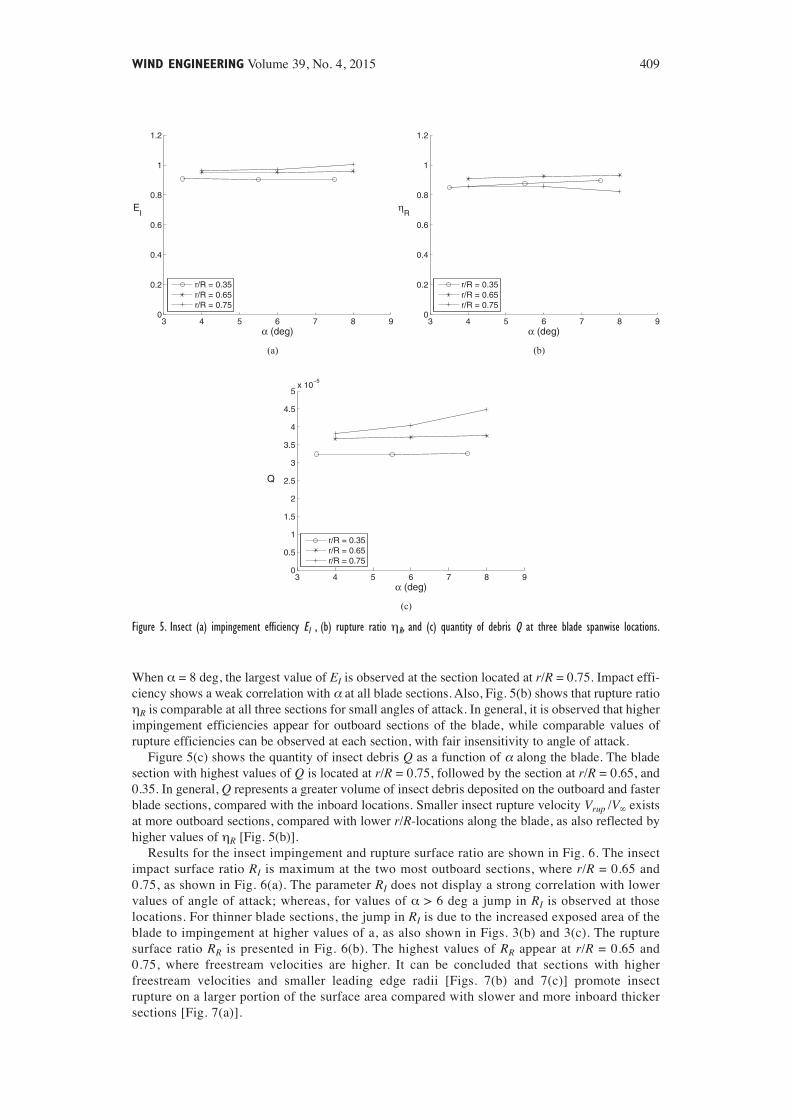
When α = 8 deg, the largest value of EI is observed at the section located at r/R = 0.75. Impact effi-ciency shows a weak correlation with α at all blade sections. Also, Fig. 5(b) shows that rupture ratioηR is comparable at all three sections for small angles of attack. In general, it is observed that higherimpingement efficiencies appear for outboard sections of the blade, while comparable values ofrupture efficiencies can be observed at each section, with fair insensitivity to angle of attack.

Figure 5(c) shows the quantity of insect debris Q as a function of α along the blade. The bladesection with highest values of Q is located at r/R = 0.75, followed by the section at r/R = 0.65, and0.35. In general, Q represents a greater volume of insect debris deposited on the outboard and fasterblade sections, compared with the inboard locations. Smaller insect rupture velocity Vrup /V∞ existsat more outboard sections, compared with lower r/R-locations along the blade, as also reflected byhigher values of ηR [Fig. 5(b)].

Results for the insect impingement and rupture surface ratio are shown in Fig. 6. The insectimpact surface ratio RI is maximum at the two most outboard sections, where r/R = 0.65 and0.75, as shown in Fig. 6(a). The parameter RI does not display a strong correlation with lowervalues of angle of attack; whereas, for values of α > 6 deg a jump in RI is observed at thoselocations. For thinner blade sections, the jump in RI is due to the increased exposed area of theblade to impingement at higher values of a, as also shown in Figs. 3(b) and 3(c). The rupturesurface ratio RR is presented in Fig. 6(b). The highest values of RR appear at r/R = 0.65 and0.75, where freestream velocities are higher. It can be concluded that sections with higherfreestream velocities and smaller leading edge radii [Figs. 7(b) and 7(c)] promote insectrupture on a larger portion of the surface area compared with slower and more inboard thickersections [Fig. 7(a)].


3 4 5 6 7 8 90

0.2

0.4

0.6

0.8

1

1.2

α (deg)

EI

r/R = 0.35r/R = 0.65r/R = 0.75

(a)

3 4 5 6 7 8 90

0.2

0.4

0.6

0.8

1

1.2

α (deg)

ηR

r/R = 0.35r/R = 0.65r/R = 0.75

(b)

3 4 5 6 7 8 90

0.5

1

1.5

2

2.5

3

3.5

4

4.5

5x 10

−5

α (deg)

Q

r/R = 0.35r/R = 0.65r/R = 0.75

(c)

Figure 5. Insect (a) impingement efficiency EI , (b) rupture ratio ηR, and (c) quantity of debris Q at three blade spanwise locations.

4.2. Sand simulationThree blade sections were simulated for sand erosion, and curves of impingement efficiency β anderosion rate E are plotted versus airfoil arc length s in Figs. 8 and 9. At r/R = 0.35 a rounded peakof β ≈ 0.9 appears in the proximity of s = 0 for all angles of attack [Fig. 8(a)]. An increment in αcauses the sand β-curve to shift toward negative values of s, indicating an increased probability ofsand impingement on the pressure side of the airfoil (s < 0). Moving toward the blade tip, the peakof β is sharper, and its maximum value is approximately 1.0, as shown in Figs. 8(b) and 8(c). Thesmaller relative thickness and nose radii of the DU 96-W-212 and –180 airfoils compared with theDU 97-W-300 airfoil yield the increase of β. When airfoil thickness is reduced, β increases inmaximum value and in growth gradient along s.

By analyzing the curves for erosion rate E in Fig. 9, a common behavior is apparent for the threeblade sections. While there are two peaks, the maximum value of E is reached on the suction sideof all airfoils (s > 0) at locations slightly aft of the leading edge. At higher angles of attack, the peak


3 4 5 6 7 8 90

0.1

0.2

0.3

0.4

0.5

0.6

0.7

0.8

0.9

1

α (deg)

RI

r/R = 0.35r/R = 0.65r/R = 0.75

(a)

3 4 5 6 7 8 90

0.1

0.2

0.3

0.4

0.5

0.6

0.7

0.8

0.9

1

α (deg)

RR

r/R = 0.35r/R = 0.65r/R = 0.75

(b)

Figure 6. Insect (a) impact surface ratio RI and (b) rupture surface ratio RR at three blade spanwise locations

Figure 7. Contours of insect normal impact velocity VN /V∞ at (a) r /R = 0.35 (α = 5.5 deg), (b) r /R = 0.65 (α = 6 deg), (c) andr /R = 0.75 (α = 6 deg); circles placed at impingement locations, triangles at rupture locations, straight segments at maximum VN /V∞.

(a)

(b)

(c)

value of E increases and appears at lower values of s, closer to the leading edge. On the pressureside of the airfoil (s < 0), a broader but lower peak of erosion rate is observed. In general, the peakvalues of erosion rate are consistently lower on the pressure side of all airfoils with respect to thepeak values at the suction side.

The values E at the blade leading edge (s = 0) are close to zero for all sections. This behavioris physical and intrinsic in the coefficients K and n used to model eqn. (30) (see Table 4). Erosionexperiments on flat-plate plastic materials show a peak in erosion rate for impact angles ≈ 30 deg,while two minima are reached for tangent (θ = 0 deg) and normal impacts (θ = 90 deg) [28, 51,56]. The present erosion simulations reflect a coherent behavior in the proximity of the stagnationline, where s ≈ 0 and θ ≈ 90 deg. When considering sand particles impinging away from suchregion, their impact velocity is higher while their impact angle is lower, which results in a peakof erosion rate at θ ≈ 22 deg. As θ approaches 0 deg, the erosion rate on the blade surfacebecomes negligible. Finally, the overall blade maximum erosion rate is reached at the mostoutboard section, located at r/R = 0.75 [Fig. 9(c)], while a value of E an order of magnitude loweris observed at r/R = 0.35 [Fig. 9(a)]. It can be concluded that given a ratio of freestream velocitiesV∞, 0.35/V∞, 0.75 ≈ 0.5, an erosion rate significantly lower is observed for the more inboard sectionof the blade.

The impact efficiency EI is plotted versus angle of attack in Fig. 10(a). As α increases, EI increaseslinearly at all three blade locations. The section showing highest values of EI is the thickest, whilethe thinnest airfoil shows the lowest values. Sand grains are lighter and smaller than insects, and thisfact is reflected by values of EI being greater than unity for the majority of test cases. An inflectionin the sand grain upper limit trajectory exists as the particle approaches the blade section. Thetrajectory inflection makes values of EI > 1 appear. The smallest envelope of sand grains is capturedby the blade sections at r/R = 0.65 and 0.75. On the other hand, by analyzing Fig. 10(b), maximum


−1.2 −1 −0.8 −0.6 −0.4 −0.2 0 0.2 0.40

0.1

0.2

0.3

0.4

0.5

0.6

0.7

0.8

0.9

1

s

β

α = 3.5 degα = 5.5 degα = 7.5 deg

(a)

−1.2 −1 −0.8 −0.6 −0.4 −0.2 0 0.2 0.40

0.1

0.2

0.3

0.4

0.5

0.6

0.7

0.8

0.9

1

s

β


(b)

−1.2 −1 −0.8 −0.6 −0.4 −0.2 0 0.2 0.40

0.1

0.2

0.3

0.4

0.5

0.6

0.7

0.8

0.9

1

s

β


(c)

Figure 8. Sand β curves at a r /R of (a) 0.35, (b) 0.65, and (c) 0.75

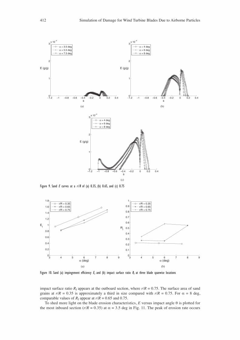
impact surface ratio RI appears at the outboard section, where r/R = 0.75. The surface area of sandgrains at r/R = 0.35 is approximately a third in size compared with r/R = 0.75. For α = 8 deg,comparable values of RI appear at r/R = 0.65 and 0.75.

To shed more light on the blade erosion characteristics, E versus impact angle θ is plotted forthe most inboard section (r/R = 0.35) at α = 3.5 deg in Fig. 11. The peak of erosion rate occurs


−1.2 −1 −0.8 −0.6 −0.4 −0.2 0 0.2 0.40

1

2

3x 10

−4

s

E (g/g)

α = 3.5 degα = 5.5 degα = 7.5 deg

(a)

−1.2 −1 −0.8 −0.6 −0.4 −0.2 0 0.2 0.40

1

2

3x 10

−4

s

E (g/g)


(b)

−1.2 −1 −0.8 −0.6 −0.4 −0.2 0 0.2 0.40

1

2

3x 10

−4

s

E (g/g)


(c)

Figure 9. Sand E curves at a r /R of (a) 0.35, (b) 0.65, and (c) 0.75

3 4 5 6 7 8 90

0.2

0.4

0.6

0.8

1

1.2

1.4

1.6

1.8

α (deg)

EI

r/R = 0.35r/R = 0.65r/R = 0.75

(a)

3 4 5 6 7 8 90

0.1

0.2

0.3

0.4

0.5

0.6

0.7

0.8

0.9

1

α (deg)

RI

r/R = 0.35r/R = 0.65r/R = 0.75

(b)

Figure 10. Sand (a) impingement efficiency EI and (b) impact surface ratio RI at three blade spanwise locations

at θ = 22 deg, for both upper and lower blade sides. The role played by the distribution of impactvelocity around the curved surface of the blade is apparent. A larger value of E is observed on theblade upper side where dynamic pressure is higher, as opposed to the blade lower side, where Eis lower. Such behavior is correlated to the velocity flowfield around the blade section.

A broader range of negligible erosion rate in the vicinity of the stagnation point is observedat r/R = 0.35, as shown in Fig. 12(a), compared with thinner and more outboard sections [seeFigs. 12(b) and 12(c)]. On the other hand, a wider range of negligible erosion rate is observedon the blade pressure side at r/R = 0.75 [Fig.12(c)] as compared with more inboard sections.When moving toward the blade tip, both of the peaks in E increase in value and move towardthe blade leading edge, particularly the pressure side peak.


Figure 11. Sand erosion rate E at r /R = 0.35 and α = 3.5 deg

Figure 12. Contours of sand erosion rate E at (a) r /R = 0.35 (α = 5.5 deg), (b) r /R = 0.65 (α = 6 deg), and (c) r /R = 0.75(α = 6 deg), where the black circles are placed at sand grain impact locations, and the grey circles indicate maximum E on theblade suction and pressure sides

(a)

(b)

(c)

The result of a continuous erosion produced by sand grains may appear as core composite materialexposure in the vicinity of the blade leading edge, where E has a maximum. However, the erosionmechanism associated with composite matrix materials used for wind turbine blades [57, 58]typically shows maximum erosion rate for θ in the range of 45–55 deg [59–61]. In general, compositematrix materials have different erosion constants K and n compared with the outer coating.

A proposed model to explain operational damage to blades due to airborne particles is as follows:

1. Particles collide mainly in the proximity of the blade leading edge. The maximum observedinsect debris thickness is close to the blade stagnation point; whereas, sand grains collidewith the blade surface and promote two erosion peaks downstream of the stagnation point,where impact angles reach ≈ 22 deg.

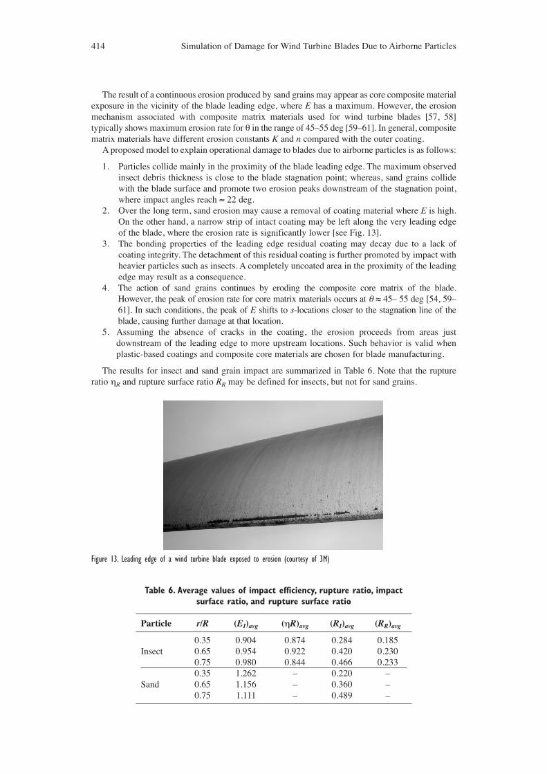
2. Over the long term, sand erosion may cause a removal of coating material where E is high.On the other hand, a narrow strip of intact coating may be left along the very leading edgeof the blade, where the erosion rate is significantly lower [see Fig. 13].

3. The bonding properties of the leading edge residual coating may decay due to a lack ofcoating integrity. The detachment of this residual coating is further promoted by impact withheavier particles such as insects. A completely uncoated area in the proximity of the leadingedge may result as a consequence.

4. The action of sand grains continues by eroding the composite core matrix of the blade.However, the peak of erosion rate for core matrix materials occurs at θ ≈ 45– 55 deg [54, 59–61]. In such conditions, the peak of E shifts to s-locations closer to the stagnation line of theblade, causing further damage at that location.

5. Assuming the absence of cracks in the coating, the erosion proceeds from areas justdownstream of the leading edge to more upstream locations. Such behavior is valid whenplastic-based coatings and composite core materials are chosen for blade manufacturing.

The results for insect and sand grain impact are summarized in Table 6. Note that the ruptureratio ηR and rupture surface ratio RR may be defined for insects, but not for sand grains.


Figure 13. Leading edge of a wind turbine blade exposed to erosion (courtesy of 3M)

Table 6. Average values of impact efficiency, rupture ratio, impactsurface ratio, and rupture surface ratio

Particle r/R (EI)avg (ηR)avg (RI)avg (RR)avg

0.35 0.904 0.874 0.284 0.185Insect 0.65 0.954 0.922 0.420 0.230

0.75 0.980 0.844 0.466 0.2330.35 1.262 – 0.220 –

Sand 0.65 1.156 – 0.360 –0.75 1.111 – 0.489 –

5. CONCLUSIONThe present paper described simulations to evaluate operational damage of wind turbine blades due toinsects and sand grains. The trajectories of impinging particles were evaluated through a numericalcode that computed particle properties at impact. The average values of impact efficiency, ruptureratio, impact surface ratio, and rupture surface ratio along the blade were reported. Values of averageimpact efficiency EI slightly increase for insects along the span, while they decrease for sand graincollision. Average values of rupture ratio ηR are comparable at all blade sections; however, the highestvalue appears at r/R = 0.65. Another result is given by the average impact surface ratio RI whichincreases along the blade for both insects and sand grains, meaning that larger portions of the bladesurface are exposed to particle collisions. Larger rupture surface ratio RR is found at higher freestreamvelocities and thinner blade sections, meaning that a larger surface area of the blade is exposed toinsect rupture at such locations when compared with inboard locations. A similar result is given by thequantity of insect debris Q along the blade, which is also larger at outboard sections.

The erosion analysis showed that two peaks of erosion rate appear at each blade section. A higher erosion rate is reached where freestream velocities are greater. In fact, values ofmaximum erosion rate approximately ten times higher occur at r/R = 0.75 compared with the mostinboard section, r/R = 0.35 due to the nonlinear behavior of erosion rate through sand impactvelocity. This conclusion is remarkable, considering a freestream velocity approximately 50%lower at r/R = 0.35, compared with the freestream velocity at r/R = 0.75. Also, it was observed thata higher erosion rate occurs on the blade suction side, while a lower peak appears on the pressureside for the considered angles of attack. Conversely, the blade upper surface shows narrowerranges of higher erosion rate compared with lower but broader ranges on the bottom surface. Whenmoving toward the blade tip, the two peaks of erosion rate come closer and approach the bladeleading edge. In an actual case with photo record, it was observed that the first visible erosiondamage would appear at such locations.

REFERENCES[1] Dalili, N., Edrisy, A. and Carriveau, R. 2007. “A Review of Surface Engineering Issues

Critical to Wind Turbine Performance”. Renewable and Sustainable Energy Reviews, 13, pp. 428–438.

[2] Hayman, B., Wedel-Heinen, J. and Brondsted, P. 2008. “Materials Challenges in Present andFuture Wind Energy”. MRS Bulletin, 33, Apr., pp. 343–353.

[3] Singh, S., Bhatti, T. S. and Kothari, D. P. 2012. “A Review of Wind-Resource-AssessmentTechnology”. Centre for Energy Studies, Indian Institute of Technology. Hauz Khas, NewDelhi 110016.

[4] Huang, C. W., Yang, K., Liu, Q., Zhang, L., Bai, J. Y. and Xu, J. Z. 2011. “A Study onPerformance Influences of Airfoil Aerodynamic Parameters and Evalutation Indicators forthe Roughness Sensitivity on Wind Turbine Blade”. Science China - Technological Sciences,54(11), pp. 2993–2998.

[5] Siochi, E. J., Eiss, N. S., Gilliam, D. R. and Wightman, J. P. 1987. “A Fundamental Study ofthe Sticking of Insect Residues to Aircraft Wings”. Journal of Colloid and Interface Science,115(2), pp. 346–356.

[6] Croom, C. and Holmes, B. 1986. “Insect Contamination Protection for Laminar FlowSurfaces”. NASA Langley Research Center, N88-14954/7, Hampton, VA, Dec.

[7] Carmichael, B. H. 1979. “Summary of Past Experience in Natural Laminar Flow andExperimental Program for Resilient Trailing Edge”. Low Energy Transportation Systems,Capistrano Beach, CA 92624, for Ames Research Center, NASA CR 152276, May.

[8] Shankar, P. 2001. “Can Insects Seriously Affect the Power Output of Wind Turbines?”.Current Science, 81(7), pp. 747–748.

[9] Corten, G. P. and Veldkamp, H. F. 2001. “Insects can Halve Wind-Turbine Power”. Nature,412, pp. 41–42.

[10] Ragheb, A. and Selig, M. S. 2011. “Multi-Element Airfoil Configurations for WindTurbines”. In Proceedings of the 29th AIAA Conference, AIAA Paper 2011–3971.


[11] Schneiderhan, T., Schulz-Stellenfleth, J., Lehner, S. and Hortsmann, J. 2002. “Sar WindFields for Off-shore Wind Farming”. DLR, Oberpfaffenhofen, 82230 Wessling, Germany.

[12] DNV, 2010. “Design and Manufacture of Wind Turbine Blades, Offshore and Onshore WindTurbines - October 2010”. Standard DNV-DS-J102, Det Norske Veritas, Oct.

[13] Arrighetti, C., Pratti, G. D. and Ruscitti, R. 2003. “Performance Decay Analysis of NewRotor Blade Profiles for Wind Turbines Operating in Offshore Environments”. WindEngineering, 27(5), pp. 371–380.

[14] Khakpour, Y., Bardakji, S. and Nair, S. 2007. “Aerodynamic Performance of Wind TurbineBlades in Dusty Environments”. In International Mechanical Engineering Congress andExposition, Seattle, Washington, IMECE2007–43291.

[15] Tilly, G. 1969. “Erosion Caused by Airborne Particles”. Wear, 14(1), pp. 63–79.

[16] Davis, J. R., ed., 2001. Surface Engineering for Corrosion and Wear Resistance. ASMInternational - The Materials Information Society. 10M Communications, Materials Park,OH 44073-0002, ch. 3, pp. 43–86.

[17] Wood, R. J. K. 1999. “The Sand Erosion Performance of Coatings”. Materials and Design,20(4), pp. 179–191.

[18] Tabakoff, W. and Balan, C. 1983. “A Study of the Surface Deterioration due to Erosion”.Presented at the 28th ASME Interational Gas Turbine Conference and Exhibit, Phoenix,Arizona, 105, pp. 834–838.

[19] Rempel, L. 2012. “Rotor Blade Leading Edge Erosion - Real Life Experiences”. Oct. URLhttp://www.windsytemsmag.com.

[20] Sareen, A., Sapre, C. A. and Selig, M. S. 2012. “Effects of Leading-Edge Protection Tape onWind Turbine Blade Performance”. Wind Engineering, 36(5), pp. 525–534.

[21] Hayman, B., 2007. “Approaches to Damage Assessment and Damage Tolerance for FRPSandwich Structures”. Journal of Sandwich Structures and Materials, 9, pp. 571–596.

[22] Ragheb, A. M. and Ragheb, M. 2011. “Wind Turbine Gearbox Technologies”. InFundamental and Advanced Topics in Wind Power, R. Carriveau, ed. In-Tech, pp. 189–206.

[23] Ciang, C. C., Lee, J. R. and Bang, H. J. 2008. “Structural Health Monitoring for a WindTurbine System: a Review of Damage Detection Methods”. Measurement Science andTechnology, 19(12), Oct., pp. 122001–122021.

[24] Soltani, M. R., Birjandi, A. H. and Seddighi-Moorani, M. 2011. “Effect of SurfaceContamination on the Performance of a Section of a Wind Turbine Blade”. Scientia IranicaB, 18(3), pp. 349–357.

[25] Mayor, G. S., Moreira, A. B. B. and Munoz, H. C. 2013. “Influence of Roughness inProtective Strips of Leading Edge for Generating Wind Profiles”. In 22nd InternationalCongress of Mechanical Engineering, COBEM 2013.

[26] Ren, N. and Ou, J. 2009. “Dust Effect on the Performance of Wind Turbine Airfoils”.Journal of Electromagnetic Analysis and Applications, 1(2), pp. 102–107.

[27] Romero-Sanz, I. and Matesanz, A., 2008. “Noise Management on Modern Wind Turbines”.Wind Engineering, 32(1), pp. 27–44.

[28] Arjula, S. and Harsha, A. P. 2006. “Study of Erosion Efficiency of Polymers and PolymerComposites”. Polymer Testing, 25(2), pp. 188–196.

[29] Challener, C. 2010. “coatings critical for wind energy efficiency”. JCT CoatingsTech, Jan.

[30] Ragheb, M. 2010. “USA Wind Energy Resources”. University of Illinois at Urbana-Champaign, NPRE 475 lecture notes, Urbana, IL 61801, Jan.

[31] Bragg, M. B. and Maresh, J. L., 1986. A Numerical Method To Predict The Effect of InsectContamination on Airfoil Drag. Aeronautical and Astronautical Engineering Report AARL86-01, The Ohio State University Research Foundation, OH 43212, Mar.


[32] Drela, M. 1989. “XFOIL: An Analysis and Design System for Low Reynolds NumberAirfoils”. In Low Reynolds Number Aerodynamics, T. J. Mueller, ed., Vol. 54 of LectureNotes in Engineering. Springer-Verlag, New York, June, pp. 1–12.

[33] Roskam, J. 1995. Airplane Flight Dynamics and Automatic Flight Controls. DARcorp,Lawrence, KS 66044.

[34] Bragg, M. B. 1982. “Rime Ice Accretion and Its Effect on Airfoil Performance”. NASALewis Research Center, NASA CR-165599, Mar.

[35] Langmuir, I. and Blodgett, K. 1946. Mathematical Investigation of Water DropletTrajectories. Tech. Rept. 5418, U.S. Army Air Force.

[36] Hamed, A. A., Tabakoff, W., Rivir, R. B., Das, K. and Arora, P. 2005. “Turbine Blade SurfaceDeterioration by Erosion”. Journal of Turbomachinery, 127(3), pp. 445–452.

[37] Wilson, R. E. 2009. “Wind Turbine Aerodynamics Part A: Basic Principles”. In WindTurbine Technology, Fundamental Concepts of Wind Turbine Engineering, Second Edition,D. A. Spera, ed. ASME Press, Three Park Avenue, New York City, NY 10016, pp. 281–350.

[38] Timmer, W. A. and van Rooij, R. P. J. O. M. 2003. “Summary of the Delft University WindTurbine Dedicated Airfoils”. Journal of Solar Energy Engineering, 125(4), pp. 571–596.

[39] Freeman, J. 1945. “Studies in the Distribution of Insects by Aerial Currents”. Journal ofAnimal Ecology, 14(2), pp. 128–154.

[40] Nachtigall, W. 1974. Insects in Flight. HarperCollins Publishers LLC, New York.

[41] Vogel, S., 1967. “Flight in Drosophila, III, Aerodynamic Characteristics of Fly Wings andWing Models”. Journal of Experimental Biology, 46, pp. 431–443.

[42] Sun, M. and Wu, J. H. 2003. “Aerodynamic Force Generation and Power Requirements inForward Flight in a Fruit Fly with Modeled Wing Motion”. The Journal of ExperimentalBiology, 206(17), pp. 3065–3083.

[43] Hoerner, S. F. 1965. Fluid-Dynamic Drag. Hoerner Fluid Dynamics, Bakersfield, CA 93390.

[44] Nachtigall, W. 2001. “Some Aspects of Reynolds Number Effects in Animals”.Mathematical Methods in the Applied Sciences, 24, pp. 1401–1408.

[45] Lehmann, F. O. 2002. “The Constraints of Body Size on Aerodynamics and Energetics inFlying Fruit Flies: An Integrative View”. Zoology, 105(4), pp. 287–295.

[46] Haider, A. and Levenspiel, O. 1989. “Drag Coefficient and Terminal Velocity of Sphericaland Nonspherical Particles”. Powder Technology, 58(1), pp. 63–70.

[47] Coleman, W. S. 1961. “Roughness Due to Insects”. In Boundary Layer and Flow Control,G. V. Lachmann, ed., Vol. 2. Pergamon Press, pp. 682–747.

[48] Feuerstein, A. and Kleyman, A. 2009. “Ti-N Multilayer Systems for Compressor AirfoilSand Erosion Protection”. Surface and Coatings Technology, 204(6–7), pp. 1092–1096.

[49] Maozhong, Y., Baiyun, H. and Jiawen, H. 2002. “Erosion Wear Behaviour and Model ofAbradable Seal Coating”. Wear, 252(1–2), pp. 9–15.

[50] Wood, K. 2011. “Blade Repair: Closing the Maintenance Gap,” Composites World, Apr.URL http://www.compositesworld.com.

[51] Zahavi, J. and Jr., G. F. S. 1981. “Solid Particle Erosion of Polymeric Coatings”. Wear,71(2), pp. 191–210.

[52] Arjula, S., Harsha, A. P. and Ghosh, M. K. 2008. “Solid-particle Erosion Behavior of High-Performance Thermoplastic Polymers”. Journal of Material Science, 43(6), pp. 1757–1768.

[53] Harsha, A. P. and Thakre, A. A. 2007. “Investigation on Solid Particle Erosion Behaviour ofPolyetherimide and its Composites”. Wear, 262(7–8), pp. 807–818.

[54] Barkoula, N.-M. and Karger-Kocsis, J. 2002. “Review – Processes and InfluencingParameters of the Solid Particle Erosion of Polymers and Their Composites”. Journal ofMaterials Science, 37, pp. 3807–3820.


[55] Drela, M. 2014. Flight Vehicle Aerodynamics. The MIT Press, Cambridge, Massachusetts –London, England.

[56] Kharde, Y. R. and Saisrinadh, K. V. 2008. “Effect of Particle Velocity, Temperature andImpingement Angle on the Erosive Wear Behavior of Polymer Matrix Composites”.International Journal of Applied Engineering Research, 12, pp. 1689–1695.

[57] Tangler, J. L. 2000. “The Evolution of Rotor and Blade Design”. In Presented at theAmerican Wind Energy Association, Wind Power 2000, NREL CP-500-28410.

[58] Thomsen, O. T. 2009. “Sandwich Materials for Wind Turbine Blades - Present and Future”.Journal of Sandwich Structures and Materials, 11(7), pp. 7–26.

[59] Ahmed, T. J. Ninho, G. F., Bersee, H. E. N. and Beukers, A., 2009. “Improving ErosionResistance of Polymer Reinforced Composites”. Journal of Thermoplastic CompositeMaterials, 22, pp. 703–725.

[60] Drensky, G., Hamed, A., Tabakoff, W. and Abot, J. 2011. “Experimental Investigation ofPolymer Matrix Reinforced Composite Erosion Characteristics”. Wear, 270(3–4), pp. 146–151.

[61] Biswas, S. and Satapathy, A. 2009. “Erosion Wear Behavior of Polymer Composites: a Review”. Journal of Reinforced Plastics and Composites, 29, pp. 2898–2924.


Simulation of Damage for Wind Turbine Blades Due to...

Documents

Transcript of Simulation of Damage for Wind Turbine Blades Due to...