b i o s y s t e m s e n g i n e e r i n g 1 0 2 ( 2 0 0 9 ) 2 2 7 – 2 3 5

Avai lab le a t www.sc iencedi rec t .com

journa l homepage : www.e lsev ie r . com/ loca te / i ssn /15375110

Research Paper: SWdSoil and Water

Simulation of base-flow and tile-flow for stormevents in a subsurface drained watershed

Debashish Goswamia, Prasanta K. Kalitab,*aSouth West Florida Research and Education Center, University of Florida, Immokalee, FL 34142, USAbUniversity of Illinois, 1304 W. Pennsylvania Avenue, Urbana, IL 61801, USA

a r t i c l e i n f o

Article history:

Received 3 October 2007

Received in revised form

22 September 2008

Accepted 11 November 2008

Available online 18 December 2008

* Corresponding author.E-mail addresses: debashish@ufl.edu (D.

1537-5110/$ – see front matter ª 2008 IAgrEdoi:10.1016/j.biosystemseng.2008.11.004

Quantifying base-flow and tile-flow to agricultural drainage ditches is essential to under-

stand groundwater flow and nutrient dynamics in a subsurface (tile) drained watershed.

This can give an insight into the contributions of different flow components to the total

nutrient loads in a stream. MODFLOW (Groundwater Vistas) was used to simulate (steady-

state) base-flow and tile-flow for storm events in the subsurface drained Big Ditch water-

shed in Champaign County, IL, USA. A stream section of approximately 200 m in an

agricultural drainage ditch was selected for this study. Two tile drains were draining into

the stream section from both sides (north and south banks, respectively). Two cut-throat

flumes were installed at the upstream and downstream ends of the stream section to do

a mass balance of flow volumes to determine base-flow. Dataloggers and stilling basins

were connected to the flumes and tile drains to measure flow rates. Twelve wells were

installed on both sides of the channel section to measure groundwater level for model

calibration. Three storm periods were used to calibrate the model and another three storm

periods to validate it. The simulated mean hydraulic conductivity of the study site was

5.52E-04 m s�1. The mean conductance values of the tile drains flowing from north and

south banks were 6.39E-04 m2 s�1 and 2.71E-03 m2 s�1, respectively. The simulated flow

rates were within 20% of the measured rates. It may be concluded that the model simulated

base-flow and tile-flow for the storm periods successfully.

ª 2008 IAgrE. Published by Elsevier Ltd. All rights reserved.

1. Introduction not be grown economically, but subsurface drainage has both

The Midwestern states in the USA, which include Illinois, are

one of the most agriculturally productive regions in the world,

and this productivity is the result of the installation of

subsurface (tile) drainage systems. Having naturally high

water tables, many soils within the region need artificial

drainage for sustainable crop production. These drainage

systems have a significant impact on agricultural production

and water quality. Without subsurface drainage, crops could

Goswami), pkalita@uiuc.e. Published by Elsevier Ltd

positive and negative impacts. Even though it enhances the

productivity and reduces sediment and phosphorous content,

subsurface drainage increases Nitrate–N (NO3–N) delivery to

the receiving water bodies (Fausey et al., 1995). Subsurface

drainage systems intercept nutrient rich subsurface water and

shunt it to surface water. Many studies (Baker & Johnson, 1981;

Kladivko et al., 1991; Mitchell et al., 2000) reported high NO3–N

concentrations in tile and surface waters in this region. These

concentrations are much higher than the maximum

du (P.K. Kalita).. All rights reserved.

b i o s y s t e m s e n g i n e e r i n g 1 0 2 ( 2 0 0 9 ) 2 2 7 – 2 3 5228

contaminant level (MCL) of 10 mg l�1 set by the US Environ-

mental Protection Agency (EPA). Nitrate–N is mobile and it can

be lost from the soil profile by leaching. When groundwater

flows to surface water bodies, or where soil is drained artifi-

cially, NO3–N leached to the root zone tends to end up in

surface water (Mitchell et al., 2000). Nitrogen (N) loading to the

Gulf of Mexico has increased in the last decades and the agri-

culturally dominant regions in the Midwest are a major source

of N to the Mississippi River (Goolsby et al., 2001). Massive NO3–

N loss from Midwestern states has caused serious water

quality problems and is responsible for the increase in the

hypoxic zone in the Gulf of Mexico (Jaynes et al., 2004).

Efforts are continuing to understand the nutrient dynamics

in subsurface drained watersheds and the nutrient contribu-

tions by tile-flow and base-flow to agricultural ditches. During

the last decade, developments in understanding the

hydrology of subsurface drained watersheds with intense tile-

drained systems have raised questions about the hydrology

and water quality (Mitchell et al., 2000). To study the effects of

tile drains on water quality, quantification of nutrients deliv-

ered by tile drains and other flow processes (e.g. base-flow and

runoff) to water bodies is necessary. To determine nutrient

loads, quantifying the various flow components is essential.

Models might be useful to simulate these flow components

and study different flow scenarios.

In this research, MODFLOW (United States Geological

Survey, USA) was used in a graphical user interface called

Groundwater Vistas (Environmental Simulations Inc., USA) to

simulate tile-flow and base-flow. MODFLOW is a three-

dimensional finite-difference model (McDonald & Harbaugh,

1988) which uses a block-centred approach and a modular

structure consisting of a main program and a series of sub-

routines grouped into packages. Groundwater Vistas (GW

Vistas) supports several commonly used groundwater flow

and solute transport modelling programs including MOD-

FLOW. It is also equipped with programs for sensitivity anal-

ysis, parameter estimation, and management optimisation

(ESI, 2004; Langevin & Bean, 2005). However, very little

research is available in the literature describing the simula-

tion of tile drains using MODFLOW in GW Vistas interface.

Models have been used in different studies to simulate tile-

flow and other groundwater flow components in subsurface

drained watersheds. Samani et al. (2006) proposed an analyt-

ical method to directly evaluate discharge from tile drains in

an unconfined aquifer. To verify the accuracy of the analytical

solution, MODFLOW 2000 (Harbaugh et al., 2000) was used. The

drain feature in MODFLOW was originally developed to

simulate agricultural drainage tiles that remove water from an

aquifer at a rate proportional to the difference in water level,

or head, between the aquifer and the drain elevation, as long

as the head in the aquifer is above the tile drain elevation

(Harbaugh et al., 2000; Mohamed & Rushton, 2006; Samani

et al., 2006). If the head in the aquifer falls below the drain

elevation, no additional water would be removed (Quinn et al.,

2006). Vrugt et al. (2004) used the same relationship in a model

called MODHMS, an extension of MODFLOW.

Ballaron (1998) developed a model to evaluate the ability of

field drains to study groundwater contamination using

MODFLOW. Because of the lack of adequate field data, the

model used a hypothetical field-drain site under steady-state

conditions, having physical parameters similar to an actual

drain site. Constant head nodes were used to represent the

water table gradient and a discharge zone. The drain was

simulated using the drain package available in MODFLOW-96.

An initial value of drain conductivity from the literature was

used and it was adjusted by trial and error, comparing the

simulated and measured discharges. Mohamed & Rushton

(2006) reported that to simulate tile drains in a shallow

aquifer, three component mechanisms need to be considered

and these are (1) groundwater flow in the shallow aquifer with

appropriate boundary conditions, (2) flows from the aquifer

into the horizontal well, (3) hydraulic conditions within the

horizontal well.

Model calibration with GW Vistas can be carried out using

either the traditional trial and error approach or the model-

independent calibration software such as PEST (Watermark

Numerical Computing, Australia) and UCODE (Universal

Inverse Code; United States Geological Survey, USA) which are

embedded in GW Vistas. GW Vistas is also equipped with its

own automatic calibration utilities for MODFLOW. During the

calibration process, GW Vistas provides a number of calibration

statistics, as well as plots of observed and simulated values

(Langevin & Bean, 2005). In this paper, steady-state MODFLOW

(GW Vistas) was used to simulate tile-flow and base-flow for

storm periods in a subsurface (tile) drained watershed.

2. Materials and methods

2.1. Study area description

This study was carried out on the Big Ditch watershed in

Champaign County, IL, USA. The Big Ditch has an area of

9842 ha and is a sub-watershed of the Lake Decatur water-

shed. There are five major types of soils found in the water-

shed, the most significant of which are poorly drained

Drummer and Sable silty clay loams and somewhat poorly

drained Flanagan and Ipava silt loams (Demissie & Keefer,

1996). A channel section of 200 m in length with two tile

outlets was chosen at the site (Fig. 1). Surface runoff rarely

occurs in these watersheds due to flat topography (Mitchell

et al., 2002). Therefore, base-flow and tile-flow were the only

sources of flow contribution within the channel section.

2.2. Stream-flow monitoring

To measure the amounts of water flowing in and out of the

section cut-throat flumes (ASABE Standards, 2001) were

installed at the upstream and downstream ends of the

channel section. Water levels in each flume were recorded by

a data logger (12-bit, 2-channel), which was connected to

potentiometers driven by float-counterweights inside the

stilling basins. The output voltage signals of the potentiome-

ters were directly related to the changes in the water levels in

the flumes. Flow rates at the flumes were calculated using the

equations presented by Skogerboe et al. (1967, 1973).

2.3. Tile-flow monitoring

Each tile outlet was connected to a stilling basin, which had

a potentiometer driven by a float-counterweight. As the float

Fig. 1 – Experimental site layout at the Big Ditch watershed.

b i o s y s t e m s e n g i n e e r i n g 1 0 2 ( 2 0 0 9 ) 2 2 7 – 2 3 5 229

moved with variations in water level, the potentiometer

provided different output signals for the data logger. To

convert these signals to tile-flow rates, a calibration curve was

developed for each tile drain using the output signals and the

corresponding known flow rates.

2.4. Determination of base-flow using mass balancemethod

A mass balance approach was used to calculate the base-flow

contribution within the channel section. The base-flow

volume was estimated by subtracting the flow entering the

upstream flume and the tile-flow volumes from the flow

measured at the downstream flume. Lander et al. (2005) and

Cey et al. (1998) used similar relationships to estimate base-

flow.

2.5. Water table monitoring

Twelve wells were installed on both sides of the channel

section as shown in Fig. 1. Water table depths in the wells

were measured using a water level meter (Solinst Canada

Ltd.). The water table data and topographic survey data were

used to derive the actual water table elevations from

a common datum. The datum (zero elevation) coincided with

the bottom of the unconfined aquifer.

2.6. Tile-flow simulation

The drain software package in MODFLOW can be used to

simulate flow conditions for both closed and open drains.

When the head (h) in the aquifer is higher than the drain

elevation (d ), the drain removes water from the model at

a rate (Q) calculated using the conductance (C ) of the drain

and difference between aquifer head (h) and the drain eleva-

tion (d ) as follows (Anderson & Woessner, 1992).

Q ¼ 0 for h � d (1)

Q ¼ Cðh� dÞ for h > d (2)

A tile drain can be considered as a closed drain with

perforations in it. For a closed drain, the conductance is

influenced by the size and density of openings in the drain, the

chemical precipitation around the drain, hydraulic conduc-

tivity, and the thickness of backfill around the drain (Ballaron,

1998). In the above equation, Q, h, and d are known from field

measurements, only unknown term being C. This is the

conductance of the tile drain and can be estimated by model

calibration.

2.7. Steady-state model to simulatebase-flow and tile-flow

GW Vistas supports four types of head-dependent flux

boundary conditions, which include drain, river, general-

head, and stream. The head-dependent flux boundary condi-

tion computes the flux of water into or out of the model and

assigns that flux to the cell. A constant head boundary

condition can be applied at the locations in the model where

the head does not vary during the entire simulation. For

steady-flow simulations, the constant head boundary condi-

tions provide flux to the flow system. In the model, constant

head boundaries were set at the north and the south bound-

aries approximately 500 m away from the stream segment

(Fig. 2). Constant heads were installed at sufficient distances

away so that these did not affect the flow fields near the

drains.

Six storm periods of one-day duration were chosen from

six different storm events used for this study. The storm

periods were chosen such that the heads in the wells

remained unchanged for the one-day durations. This was

confirmed from the head measurement data for two consec-

utive days. Water levels in the wells were measured once

a day. This period was expected to have constant heads at the

model boundaries in the north and the south. A field-

measured mass balance, based on the upstream, downstream

and tile hydrographs for these one-day periods, confirmed the

nearly constant base-flow rates. Head does not change with

time in a steady-state flow system. In MODFLOW, the

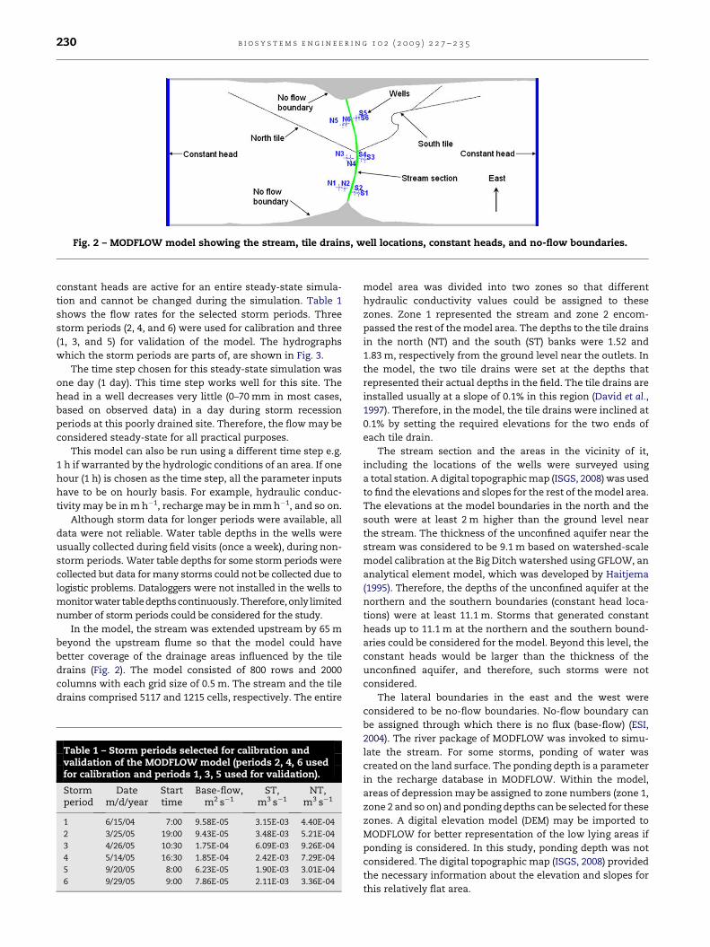
Fig. 2 – MODFLOW model showing the stream, tile drains, well locations, constant heads, and no-flow boundaries.

b i o s y s t e m s e n g i n e e r i n g 1 0 2 ( 2 0 0 9 ) 2 2 7 – 2 3 5230

constant heads are active for an entire steady-state simula-

tion and cannot be changed during the simulation. Table 1

shows the flow rates for the selected storm periods. Three

storm periods (2, 4, and 6) were used for calibration and three

(1, 3, and 5) for validation of the model. The hydrographs

which the storm periods are parts of, are shown in Fig. 3.

The time step chosen for this steady-state simulation was

one day (1 day). This time step works well for this site. The

head in a well decreases very little (0–70 mm in most cases,

based on observed data) in a day during storm recession

periods at this poorly drained site. Therefore, the flow may be

considered steady-state for all practical purposes.

This model can also be run using a different time step e.g.

1 h if warranted by the hydrologic conditions of an area. If one

hour (1 h) is chosen as the time step, all the parameter inputs

have to be on hourly basis. For example, hydraulic conduc-

tivity may be in m h�1, recharge may be in mm h�1, and so on.

Although storm data for longer periods were available, all

data were not reliable. Water table depths in the wells were

usually collected during field visits (once a week), during non-

storm periods. Water table depths for some storm periods were

collected but data for many storms could not be collected due to

logistic problems. Dataloggers were not installed in the wells to

monitor water tabledepthscontinuously. Therefore,only limited

number of storm periods could be considered for the study.

In the model, the stream was extended upstream by 65 m

beyond the upstream flume so that the model could have

better coverage of the drainage areas influenced by the tile

drains (Fig. 2). The model consisted of 800 rows and 2000

columns with each grid size of 0.5 m. The stream and the tile

drains comprised 5117 and 1215 cells, respectively. The entire

Table 1 – Storm periods selected for calibration andvalidation of the MODFLOW model (periods 2, 4, 6 usedfor calibration and periods 1, 3, 5 used for validation).

Stormperiod

Datem/d/year

Starttime

Base-flow,m2 s�1

ST,m3 s�1

NT,m3 s�1

1 6/15/04 7:00 9.58E-05 3.15E-03 4.40E-04

2 3/25/05 19:00 9.43E-05 3.48E-03 5.21E-04

3 4/26/05 10:30 1.75E-04 6.09E-03 9.26E-04

4 5/14/05 16:30 1.85E-04 2.42E-03 7.29E-04

5 9/20/05 8:00 6.23E-05 1.90E-03 3.01E-04

6 9/29/05 9:00 7.86E-05 2.11E-03 3.36E-04

model area was divided into two zones so that different

hydraulic conductivity values could be assigned to these

zones. Zone 1 represented the stream and zone 2 encom-

passed the rest of the model area. The depths to the tile drains

in the north (NT) and the south (ST) banks were 1.52 and

1.83 m, respectively from the ground level near the outlets. In

the model, the two tile drains were set at the depths that

represented their actual depths in the field. The tile drains are

installed usually at a slope of 0.1% in this region (David et al.,

1997). Therefore, in the model, the tile drains were inclined at

0.1% by setting the required elevations for the two ends of

each tile drain.

The stream section and the areas in the vicinity of it,

including the locations of the wells were surveyed using

a total station. A digital topographic map (ISGS, 2008) was used

to find the elevations and slopes for the rest of the model area.

The elevations at the model boundaries in the north and the

south were at least 2 m higher than the ground level near

the stream. The thickness of the unconfined aquifer near the

stream was considered to be 9.1 m based on watershed-scale

model calibration at the Big Ditch watershed using GFLOW, an

analytical element model, which was developed by Haitjema

(1995). Therefore, the depths of the unconfined aquifer at the

northern and the southern boundaries (constant head loca-

tions) were at least 11.1 m. Storms that generated constant

heads up to 11.1 m at the northern and the southern bound-

aries could be considered for the model. Beyond this level, the

constant heads would be larger than the thickness of the

unconfined aquifer, and therefore, such storms were not

considered.

The lateral boundaries in the east and the west were

considered to be no-flow boundaries. No-flow boundary can

be assigned through which there is no flux (base-flow) (ESI,

2004). The river package of MODFLOW was invoked to simu-

late the stream. For some storms, ponding of water was

created on the land surface. The ponding depth is a parameter

in the recharge database in MODFLOW. Within the model,

areas of depression may be assigned to zone numbers (zone 1,

zone 2 and so on) and ponding depths can be selected for these

zones. A digital elevation model (DEM) may be imported to

MODFLOW for better representation of the low lying areas if

ponding is considered. In this study, ponding depth was not

considered. The digital topographic map (ISGS, 2008) provided

the necessary information about the elevation and slopes for

this relatively flat area.

Fig. 3 – Storms from which the calibration and validation periods were chosen. upstream hydrograph,

downstream hydrograph, ST flow hydrograph, NT flow hydrograph (date format: month/day/year).

b i o s y s t e m s e n g i n e e r i n g 1 0 2 ( 2 0 0 9 ) 2 2 7 – 2 3 5 231

2.8. Calibration of the model for storm periods

For calibration of the model, storm periods 2, 4, and 6 were

chosen (Table 1, Fig. 3). An AutoCAD drawing of the stream with

the 12 wells was imported to the model so that the exact loca-

tions of the stream and the wells could be assigned in the

model. The heads in the wells were used as targets for cali-

bration. Targets are points in space and time domain, where

the model dependent variables are measured (ESI, 2004). The

sensitivity analysis provides an error term, called the residual

for each target location. A residual is the difference between the

measured and simulated parameter values for a target. The

sum of squared residuals (SSR) is computed by squaring

the residuals for the targets and then adding these together. The

basic objective of calibration is to lower the SSR keeping

the parameters within reasonable ranges. The calibration

process of a model involves identification of the most sensitive

parameters, and based on the sensitivity analyses, determina-

tion of the calibrated values of these parameters. The model

was calibrated using a manual trial and error adjustment of

parameters and UCODE. UCODE performs inverse modelling

using non-linear regression (Poeter & Hill, 1998). Based on the

sensitivity study, the model parameters considered for cali-

brations were hydraulic conductivity, recharge, constant head

and tile drain conductance.

The lengths of the main tiles for NT and ST were 360 and

406 m, respectively as determined from Geographic Informa-

tion System (GIS) maps by the method explained by Verma

et al. (1996) (Fig. 4). NT did not have any lateral drain. The

drainage area of ST was shared by another tile network with

its outlet outside of the stream section under study. As far as

the simulation of ST was concerned, the calibration of the

model based on the heads in the wells near the stream section

and the flow rates (base-flow and tile-flow) took care of any

water loss from the model area by the tile drain which was

sharing the same drainage area with ST. The calibrated

conductance of ST reflected its ability to drain water from the

drainage area it shared with the other tile drain. In other

words, the conductance of ST would have been larger if there

were no other tile drains present in the same drainage area.

The rainfall measured by the rain gauge cannot be used in

MODFLOW (GW Vistas). The rainfall amount that translates

into base-flow and tile-flow should be used in the model. This

rainfall (recharge) amount had to be calibrated for the model.

Fig. 4 – Tile networks generated from GIS maps.

Table 2 – Calibrated parameters for the model.

Parameter Unit Period 2 Period 4 Period 6

Constant head (North) m 9.69 10.21 9.13

Constant head (South) m 9.60 9.50 8.92

Recharge mm d�1 6.80 9.40 3.92

Hydraulic conductivity

(for zone 1)

m s�1 9.84E-06 1.10E-05 9.72E-06

Hydraulic conductivity

(for zone 2)

m s�1 5.21E-04 6.37E-04 4.98E-04

Conductance (NT) m2 s�1 6.48E-04 5.09E-04 7.59E-04

Conductance (ST) m2 s�1 2.88E-03 1.98E-03 3.28E-03

Table 3 – Watershed-scale hydraulic conductivity valuesfrom different studies.

Reference Calibrated hydraulicconductivity (m s�1)

Sloan (2000) 9.26E-04

Barlow et al. (2003) 7.06E-04

Roadcap & Wilson (2001) 9.88E-04

Modica & Buxton (1998) 7.06E-04

Rodriguez et al. (2006) 3.99E-03

b i o s y s t e m s e n g i n e e r i n g 1 0 2 ( 2 0 0 9 ) 2 2 7 – 2 3 5232

Evapotranspiration (ET) was also not considered for the

model. The model can be run without incorporating ET, but for

more accuracy ET could be considered. The hydraulic

conductivity of the stream bed is usually lower than that of

rest of the watershed due to the deposition of silt, clay and

organic materials (Fox, 2003; Chen, 2004). Therefore, this

parameter was also calibrated.

2.9. Validation of the model for storm periods

To evaluate the ability of the model to simulate flows, a simple

equation (Eq. (3)) was used to determine the percentage

difference (absolute value) between measured and simulated

flow rates. Similar comparisons were made by many

researchers to test the validity of their models as mentioned in

sub-Section 3.2.

Percentage difference ðabsolute valueÞ

¼

0@

ffiffiffiffiffiffiffiffiffiffiffiffiffiffiffiffiffiffiffiffiffiffiffiffiffiffiffiffiffiffiffiffiffiffiffiffiffiffiffiffiffiffiffiffiffiffiffiffiffiffiffiffiffiffiffiffiffiffiðObserved� SimulatedÞ2

q

Observed

1A100% (3)

3. Results and discussion

3.1. Calibration results for the model

The calibrated values of the model parameters are shown in

Table 2. The calibrated hydraulic conductivity values for the

watershed site were found to be higher than that estimated by

slug tests for similar soils. Mehnert et al. (2005) found median

hydraulic conductivity value for the Big Ditch watershed using

slug tests to be 2.9E-06 m s�1. The hydraulic conductivity

estimated in the laboratory is usually lower than in situ

observations (Zecharias & Brutsaert, 1988). The high value of

hydraulic conductivity in the shallow geologic material might

be due to the presence of macropores, such as desiccation

cracks, root channels and worm holes (Mehnert et al., 2005).

The increase in hydraulic conductivity with larger scale is the

result of spatial heterogeneities (Rovey II, 1998) and was

described as scaling-up of hydraulic conductivity (Desbarats,

1992). There are numerous examples in literature which

reported high watershed-scale hydraulic conductivity values

for unconfined and confined aquifers. ISWS (2003) and Meh-

nert et al. (2005, 2007) reported high hydraulic conductivity

values for locations at the Big Ditch watershed by model

calibrations (1.23E-03 m s�1 and 1.32E-04 m s�1, respectively).

Table 3 shows some of the large hydraulic conductivity values

from the literature derived by model calibrations for uncon-

fined and confined aquifers.

3.2. Validation results for the model

To test the validity of the model, storm periods 1, 3, and 5 were

chosen (Table 1). MODFLOW provided a mass balance indi-

cating the amount of water entering the system (from

constant heads and recharge) and leaving the system (through

streams and tile drains). For steady-state simulations, MOD-

FLOW generates only numerical values for flow rates. GW

Vistas (version 4.0 onwards) has the ability to create a hydro-

graph for a transient model that summarizes the changes in

flux over time (ESI, 2004). The average hydraulic conductivity

values for zones 1 and 2, and average conductance values for

the two tile drains estimated by model calibrations (Table 4)

were used to validate the model. These values were constants

for this model. The constant heads and recharge had to be

calibrated for each storm during the validation process. These

were calibrated using the heads in the wells as targets. The

MODFLOW model direction of groundwater flow and head

contours (in m) for storm period 1 are shown in Fig. 5. Table 5

shows the measured and simulated flow rates and the

Table 4 – Calibrated parameters used for validation of themodel.

Parameter Calibrated values(arithmetic mean)

Hydraulic conductivity (for zone 1) 1.02E-05 m s�1

Hydraulic conductivity (for zone 2) 5.52E-04 m s�1

Conductance (NT) 6.39E-04 m2 s�1

Conductance (ST) 2.71E-03 m2 s�1

b i o s y s t e m s e n g i n e e r i n g 1 0 2 ( 2 0 0 9 ) 2 2 7 – 2 3 5 233

percentage differences for the measured and simulated flow

rates for the three storm periods used in the validation. The

simulated flow rates were within 20% of the measured values.

Only two studies (Cey et al., 1998; Lander et al., 2005)

appear to be available that report the separation of base-flow

within a stream section in subsurface (tile) drained water-

sheds based on upstream and downstream hydrographs and

no model was tested based on those data. No data was found

in the literature which applied MODFLOW (GW Vistas) to

separate base-flow and tile-flow for Midwestern watersheds

although several other models have been developed to

simulate water movements associated with tile drainage.

These drainage models simulate parallel tile systems, even

though many existing tile systems are not parallel and are

distributed in a more or less random geometrical pattern

(Sogbedji & McIsaac, 2002). Most investigations, both theo-

retical and experimental, have focused on parallel drainage

systems with equally spaced tiles (Cooke et al., 2001).

However, in many watersheds, such as the Big Ditch in Illi-

nois, parallel systems do not occur as frequently as irregular

systems. MODFLOW can be used for tile networks of any

geometric pattern.

Arnold & Allenb (1996) used SWAT (Soil and Water

Assessment Tool) model in Illinois watersheds. Most of the

simulated flow components (surface and ground water) were

within 5% and nearly all were within 25% of the measured

values. Du et al. (2005) modified SWAT model by associating it

with a simple tile-flow equation to simulate water table

dynamics. The modified SWAT model (SWAT-M) was evalu-

ated using measured flow data from Walnut Creek watershed,

an intensively tile-drained watershed in central Iowa, a Mid-

western state. For validation period, the percentage differ-

ences for monthly and daily mean flow rates were 8.5 and 7.7%

less as compared to the measured values.

Fig. 5 – MODFLOW showing the groundwater flow

Davis et al. (2000) applied ADAPT (Agricultural Drainage

and Pesticide Transport) model to simulate tile drains in

Minnesota, a Midwestern state. The model over-predicted the

total tile-drainage by 8.8%. Drainage Model (DRAINMOD) is

a field-scale, water management simulation model developed

by Skaggs (1980). DRAINMOD-N is an extension to DRAINMOD

to predict nitrogen fate and transport from subsurface drainage

systems (Breve et al., 1997). Northcott et al. (2001) used DRAIN-

MOD-N to simulate flow for irregular tile drains in the flat

watersheds of East Central Illinois. To use the model on irregu-

larly spaced tile systems, effective drain spacing was calibrated.

They found that the average absolute daily deviation between

measured and observed flow was 23.9 m3 day�1 (0.89 mm

day�1). There was no reference to the percentage difference

between measured and simulated flow rates.

GLEAMS (Groundwater Loading Effects of Agricultural

Management Systems) is a water quality model that has

hydrology, erosion, pesticide, and nutrient as sub-models

(Leonard et al., 1987). Shirmohammadi et al. (1998) reported

that GLEAMS was capable of simulating drainage discharge in

a subsurface (tile) drained watershed. Bakhsh et al. (1999) used

GLEAMS to simulate tile drains and nitrate–N (NO3–N) loss

from subsurface (tile) drained watersheds in Iowa. The model

predicted subsurface flows with a relative error of 6.2%.

Overall, the model under-predicted the observed tile-flow

by 15%.

In this study, because of the limited data available, only

three storm periods were used and the model could not be

tested for wide variety of storms. Also, many statistical anal-

yses could not be performed with limited number of data

points. Therefore, to evaluate the model the percentage

differences between measured and simulated flow rates were

calculated. This is a simple and common method to test

a model. Winter (1981) found that long-term averages had less

error than short-term values. Errors in annual estimates of

precipitation, stream flow and evaporation ranged from 2 to

15% whereas monthly estimates ranged from 2 to 30%. The

MODFLOW model in our study simulated flow rates on daily

basis within 20% error. The model was calibrated and vali-

dated using storm periods with different water table eleva-

tions and recharge rates. It may be concluded that the model

could simulate base-flow and tile-flow successfully even

though more simulations are required to evaluate how robust

the model is. In future, to better calibrate and validate the

model, data should be collected for more storms. Similar

directions and head contours (storm period 1).

Table 5 – Measured and simulated flow rates (base-flow and tile-flow) for the storm periods used for validation of themodel.

StormPeriod

Base-flowmeasured, m2 s�1

Simulated,m2 s�1

% Diff ST measured,m3 s�1

Simulated,m3 s�1

% Diff NT measured,m3 s�1

Simulated,m3 s�1

% Diff

1 9.58E-05 9.12E-05 4.9 3.15E-03 2.59E-03 17.6 4.40E-04 5.21E-04 18.4

3 1.75E-04 1.41E-04 19.3 6.09E-03 5.57E-03 8.6 9.26E-04 1.08E-03 16.3

5 6.23E-05 6.97E-05 11.9 1.90E-03 1.69E-03 11.0 3.01E-04 2.55E-04 15.3

Mean 12.0 12.4 16.7

b i o s y s t e m s e n g i n e e r i n g 1 0 2 ( 2 0 0 9 ) 2 2 7 – 2 3 5234

models could also be developed for other subsurface (tile)

drained sites.

3.3. Relating the model results to water quality data todetermine nutrient loads

Once the base-flow and tile-flow rates are known, the corre-

sponding nutrient loadings to the streams can be calculated.

The nutrient concentrations in the water samples (collected

from tile and groundwater wells) and the corresponding flow

(tile-flow and base-flow) rates can be used to calculate the

instantaneous loads as shown below.

Li ¼ Ci � Qi (4)

where Li, Ci and Qi are the instantaneous load, nutrient

concentration, and flow rate at the i-th time period, respec-

tively (Bowes & House, 2001; Bowes et al., 2005). Water samples

collected from groundwater wells may be used to quantify

nutrient loads contributed by base-flow. The flow rates can be

associated with water quality data to quantify nutrient loads.

There is no limitation in extending MODFLOW to water

quality in subsurface (tile) drained watersheds.

4. Conclusions

A model was developed using MODFLOW (GW Vistas) to

simulate flow (base-flow and tile-flow) for storm periods in

a subsurface drained watershed. The tile drains at the site were

of irregular shape. Unlike many other models, one advantage

of MODFLOW is that it can be used to simulate tile drains of any

geometric pattern. Because data was available for only for

a few storms, the model could not be used for a wide variety of

storms involving all seasons. Three storm periods were used to

calibrate the model and another three storm periods to vali-

date it. The simulated flow rates (base-flow and tile-flow) were

within 20% of the measured rates. Based on the calibration and

validation of the model with storm periods having different

water table elevations and recharge rates, it may be concluded

that the model could simulate the flow rates successfully.

In the future, data for additional storm periods should be

collected to evaluate the model for various flow conditions

throughout the year. The ET rate was not incorporated in the

model. For more accuracy in model calibration and validation,

the ET rate should be considered. Storms that generate

constant heads equal to the thickness of the unconfined

aquifer or lower may be considered for simulation using this

model. Once the flow rates are estimated using the model,

these data can be associated with the corresponding nutrient

concentrations and used to calculate the nutrient loads.

r e f e r e n c e s

Anderson M P; Woessner W W (1992). Applied GroundwaterModeling: Simulation of Flow and Advective Transport.Academic Press, San Diego, California.

Arnold J G; Allenb P M (1996). Estimating hydrologic budgetsfor three Illinois watersheds. Journal of Hydrology, 176,57–77.

ASABE Standards (2001). S526.2: Soil and Water Terminology.ASABE, St. Joseph, MI.

Baker J L; Johnson H P (1981). Nitrate–nitrogen in tile drainage asaffected by fertilization. Journal of Environmental Quality, 10,519–522.

Bakhsh A; Kanwar R S; Jaynes D B; Colvin T S; Ahuja L R (1999).Prediction of NO3–N losses with subsurface drainage waterfrom manured and UAN-fertilized plots using GLEAMS.Transactions of the ASABE, 43(1), 69–77.

Ballaron P B (1998). Use of a Field Drain and an Artificial Wetlandto Minimize Groundwater Contamination from anAgricultural Site. Publication no. 197. Susquehanna RiverBasin Commission, Harrisburg, Pennsylvania.

Barlow P M; Ahlfeld D P; Dickerman D C (2003). Conjunctive-management models for sustained yield of stream-aquifersystems. Journal of Water Resources Planning andManagement, 129(1), 35–48.

Bowes M J; House W A (2001). Phosphorous and dissolved silicondynamics in the River Swale catchment, UK: a mass-balanceapproach. Hydrological Processes, 15, 261–280.

Bowes M J; Leach D V; House W A (2005). Seasonal nutrientdynamics in a chalk stream: the River Frome, Dorset, UK.Science of the Total Environment, 336, 225–241.

Breve M A; Skaggs R W; Parsons J E; Gilliam J W (1997).DRAINMOD–N: a nitrogen model for artificially drained soils.Transactions of ASABE, 40(4), 1067–1075.

Cey E E; Rudolf D L; Parkin G W; Aravena R (1998). Quantifyinggroundwater discharge to a small perennial stream in southOntario, Canada. Journal of Hydrology, 210, 21–37.

Chen X (2004). Streambed hydraulic conductivity for rivers insouth-central Nebraska. Journal of the American WaterResource Association, 40(3), 561–574.

Cooke R A; Badiger S; Garcıa A M (2001). Drainage equations forrandom and irregular tile drainage systems. AgriculturalWater Management, 48(3), 207–224.

David M B; Gentry L E; Kovacic D A; Smith K M (1997). Nitrogenbalance in and export from an agricultural watershed. Journalof Environmental Quality, 26, 1038–1048.

Davis D M; Gowda P H; Mulla D J; Randall G W (2000). Modelingnitrate nitrogen leaching in response to nitrogen fertilizer rateand tile drain depth or spacing for Southern Minnesota, USA.Journal of Environmental Quality, 29, 1568–1581.

Demissie M; Keefer L (1996). Watershed Monitoring and Land UseEvaluation for the Lake Decatur Watershed. Technical Report.Illinois State Water Survey, Champaign, IL.

Desbarats A J (1992). Spatial averaging of hydraulic conductivityin three-dimensional heterogeneous porous media.Mathematical Geology, 24(3), 249–267.

b i o s y s t e m s e n g i n e e r i n g 1 0 2 ( 2 0 0 9 ) 2 2 7 – 2 3 5 235

Du B; Arnold J G; Saleh A; Jaynes D B (2005). Development andapplication of SWAT to landscapes with tiles and potholes.Transactions of the ASABE, 48(3), 1121–1133.

ESI (2004). Guide to Using Groundwater Vistas. EnvironmentalSimulations Inc, Herndon, Virginia.

Fausey N R; Brown L C; Belcher H W; Kanwar R S (1995). Drainageand water quality in great lakes and cornbelt states. Journal ofIrrigation and Drainage Engineering, 121, 283–288.

Fox G A (2003). Estimating streambed and aquifer parametersfrom a stream/aquifer analysis test. In Proceedings of theTwenty-Third Annual AGU Hydrology Days. Colorado StateUniversity, Fort Collins, Colorado.

Goolsby D A; Battaglin W A; Aulenbach B T; Hooper R P (2001).Nitrogen input to the Gulf of Mexico. Journal of EnvironmentalQuality, 30, 329–336.

Haitjema H M (1995). Analytic Element Modeling of GroundwaterFlow. Academic Press, San Diego, California.

Harbaugh A W; Banta E R; Hill M C; McDonald M G (2000).MODFLOW-2000, the U.S. Geological Survey Modular Ground-water Model – User Guide to Modularization Concepts and theGround-water Flow Process. Open-File Report 00–92. U.S.Geological Survey, Reston, Virginia.

ISGS. (2008). Illinois Natural Resources Geospatial DataClearinghouse. Digital Topography Maps. Available at:<http://www.isgs.uiuc.edu/nsdihome/webdocs/drgs/drgorder24bymap.html>.

ISWS. (2003). Shallow Ground-water Flow and the Mass Flux ofNitrogen and Phosphorous in the Big Ditch Watershed. IllinoisState Water Survey, Champaign, IL. Available at: <http://www.sws.uiuc.edu/gws/docs/NPBigDitchPoster.pdf>.

Jaynes D B; Dinnes D L; Meek D W; Karlen D L; Cambardella C A;Colvin T S (2004). Using the late spring nitrate test to reducenitrate loss within a watershed. Journal of EnvironmentalQuality, 33, 669–677.

Kladivko E J; Scoyoc G E V; Monke E J; Oates K M; Pask W (1991).Pesticide and nutrient movement into subsurface tile drainson a silt loam soil in Indiana. Journal of EnvironmentalQuality, 20, 264–270.

Lander K S; Kalita P K; Cooke R A (2005). Base flow characteristicsof a subsurface-drained watershed. International AgriculturalEngineering Journal, 14(4), 171–179.

Langevin C D; Bean D M (2005). Groundwater Vistas: a graphicaluser interface for the MODFLOW family of groundwater flowand transport models. Ground Water, 43(2), 165–168.

Leonard R A; Knisel W G; Still D A (1987). GLEAMS – groundwaterloading effects of agricultural management systems.Transactions of the ASABE, 30(5), 1403–1418.

McDonald M G; Harbaugh A W (1988). A Modular Three-dimensional Finite-difference Ground-water Flow Model.Report book 6, chapter A1. USGS, Denver, CO.

Mehnert E; Dey W S; Hwang H; Keefer D A (2005). The MassBalance of Nitrogen and Phosphorus in an AgriculturalWatershed: the Shallow Groundwater Component. Open-FileSeries Report 2005-3. Illinois State Geological Survey,Champaign, IL.

Mehnert E; Hwang H; Johnson T M; Sanford R A; Beaumont W C;Holm T R (2007). Denitrification in the shallow groundwater ofa tile-drained, agricultural watershed. Journal ofEnvironmental Quality, 36, 80–90.

Mitchell J K; McIsaac G F; Walker S E; Hirschi M C (2000). Nitrate inriver and subsurface drainage flows from an East CentralIllinois watershed. Transactions of the ASABE, 43(2), 337–342.

Mitchell J K; Kalita P; Cooke R A; Hirschi M C (2002). Surface runoffoccurs only occasionally from an upland drainage watershed.

In: Proceedings of ASABE Annual Conference. Paper no.022097. St. Joseph, Michigan.

Modica E; Buxton H T (1998). Evaluating the source and residencetimes of groundwater seepage to streams, New Jersey CoastalPlain. Water Resources Research, 34(11), 2797–2810.

Mohamed A; Rushton K (2006). Horizontal wells in shallowaquifers: field experiment and numerical model. Journal ofHydrology, 329, 98–109.

Northcott W J; Cooke R A; Walker S E; Mitchell J K; Hirschi M C(2001). Application of DRAINMOD–N to fields with irregulardrainage systems. Transactions of the ASABE, 44(2), 241–249.

Poeter E P; Hill M C (1998). Documentation of UCODE, a ComputerCode for Universal Inverse Modeling. Water-resourcesInvestigations Report 98-4080. United States GeologicalSurvey, Denver, CO.

Quinn J J; Tomasko D; Kuiper J A (2006). Modeling complex flow ina karst aquifer. Sedimentary Geology, 184, 343–351.

Roadcap G S; Wilson S D (2001). The Impact of EmergencyPumpage at the Decatur Wellfields on the Mahomet Aquifer:Model Review and Recommendations. Contract Report No.2001-11. Illinois State Water Survey, Champaign, IL.

Rodriguez L B; Cello P A; Vionnet C A (2006). Modeling stream-aquifer interactions in a shallow aquifer, Choele Choel Island,Patagonia, Argentina. Hydrogeology Journal, 14, 591–602.

Rovey II C W (1998). Digital simulation of the scale effect inhydraulic conductivity. Hydrogeology Journal, 6(2), 216–225.

Samani N; Kompani-Zare M; Seyyedian H; Barry D A (2006). Flowto horizontal drains in isotropic unconfined aquifers. Journalof Hydrology, 324, 178–194.

Shirmohammadi A; Ulen B; Bergstorm L F; Knisel W G (1998).Simulation of nitrogen and phosphorus leaching ina structured soil using GLEAMS and a new submodel, PARTLE.Transactions of the ASABE, 41(2), 353–360.

Skaggs R W (1980). A Water Management Model for ArtificiallyDrained Soils. Tech. Bul. No. 267. North Carolina AgriculturalResearch Service, Raleigh, NC.

Skogerboe G M; Hyatt L; Anderson R K; Eggleston K O (1967).Design and Calibration of Submerged Open Channel FlowMeasurement Structures. Report WG 31–4. Water ResearchLaboratory, Logan, UT.

Skogerboe G; Bennett R; Walker W (1973). Selection andinstallation of cutthroat flumes for measuring irrigation anddrainage water. Experiment Station Technical Bulletin no. 120.Colorado State University, Fort Collins, CO.

Sloan W T (2000). A physics-based function for modelingtransient groundwater discharge at the watershed scale.Water Resources Research, 36(1), 225–241.

Sogbedji J M; McIsaac G F (2002). Evaluation of the ADAPT model forsimulating water outflow from agricultural watersheds withextensive tile drainage. Transactions of the ASABE, 45(3), 649–659.

Verma A K; Cooke R A; Wendte L (1996). Mapping subsurfacedrainage systems with color infrared aerial photographs. In:Proceedings of the American Water Resource Association’s32nd Annual Conference and Symposium ‘GIS and WaterResources’. Ft. Lauderdale, Florida.

Vrugt J A; Schoups G; Hopmans J W; Young C; Wallender W W;Harter T; Bouten W (2004). Inverse modeling of large-scalespatially distributed vadose zone properties using globaloptimization. Water Resources Research, 40(6), W06503.

Winter T C (1981). Uncertainties in the estimating of waterbalances of lakes. Water Resources Research, 17, 82–115.

Zecharias Y B; Brutsaert W (1988). Recession characteristics ofgroundwater outflow and base flow from mountainouswatersheds. Water Resources Research, 24(10), 1651–1658.