i

Master of Science in Applied Earth Sciences

Research Thesis

Simulation of an underground cut and fill mine

A simulation approach using SimMine to determine the systems bottlenecks and

the added value of additional miners in the production shift.

Michael van de Stadt

TU -Delft

14-01-2021

ii

Copyright © 2020 by New Boliden and Joint Master EMC European Mining Course:

Aalto University Finland, Delft University of Technology, Rheinisch - Westfalische Technische

Hochschule Aachen. All rights reserved.

No part of the material protected by this copyright notice may be reproduced or utilized in any

form or by any means, electronic or mechanical, including photocopying or by any information

storage and retrieval system, without permission from this publisher.

iii

Simulation of an underground cut and fill mine

A simulation approach using SimMine to determine the systems bottlenecks and

the added value of additional miners in the production shift.

By

Michaël van de Stadt

In partial fulfilment of the requirements for the degree of

Master of Science

In Applied Earth Sciences

At the Delft University of Technology,

To be defended publicly on the 14th

of January 2021 at 15:00

Supervisor: Dr. Masoud Soleymani Shishvan TU Delft

Dr. Rodrigo S. Guerrero Aalto

Prof. Bernd Lottermoser RWTH Aachen

Ir. Ottomar Brussee Boliden

Thesis committee: Dr. Masoud S. Shishvan TU Delft

Ir. Marco Keersemaker TU Delft

Department of Geoscience & Engineering

Delft University of Technology

An electronic version of this thesis is available at http://repository.tudelft.nl/.

iv

Abstract

As ore-bodies become more complex and difficult to extract, together with the increase towards

clean energy technologies such as wind, solar, and energy storage requires more minerals. Mining

operations need to increase their production efficiency and performance. It sounds simple, but

finding a sustainable way of achieving continuous improvement is difficult in practice. A

methodology that has been proven successful in other industries, is called the ‘theory of

constraints’. This theory focusses on the improvement change, that will make the most positive

difference, rather than making lots of small changes. Especially in underground operations, there

are many factors limiting production. In the mining industry the constraints are considered as

capacity bottlenecks, influencing the choice of the operating fleet and the usage of resources. It is

essential to identify the real bottlenecks and then develop plans to mitigate the bottlenecks.

The case study consist of a small underground mine with a small mining crew. The vehicle park

is relatively large, and therefore it is necessary to establish the added value of additional miners

or equipment for short-term production planning purposes, assuming that staff size currently

limits production capacity to find out if staff size is indeed the bottleneck in the production

capacity of the mine operation. When the bottlenecks of the mining system are known, it will be

easier to focus on necessary areas and further implementations to improve the system.

This research is aimed to fill the gaps in the literature, namely, determining the bottlenecks in an

underground cut and fill gold mine, where ore material is only transported by truck. The TOC

is a management framework used for improving system performances but doesn’t provide any

detailed analytics tools. This study compared to others is unique because it uses a simulation

study that considers: the blast cycle process, the in-mine ore and waste transport to the surface,

and the operator size.

The purpose of this study is to simulate the mining operation and identify the production

constraints, and research the influence on the number of people with the assumption that staff

sizes limit the production. The mine management is considering to add operators in the mine

production. Currently, the mine is operating on a two-shift schedule with 11 or 12 people per

shift. The mine wants to know if additional staff would increase the production of the mine with

a lower cost per tonne.

In order to investigate this problem, a literature study was conducted, and SimMine was selected

as simulation software. The first step to this approach was building a simulation model based on

the mining situation of 2019, and conducting time studies about relevant ongoing mining activities.

The necessary input data was collected by conducting activity studies during the period of March

till June of 2020 in the Kankberg-mine. By simulating the mining production cycle, using the size

of the current machine park and the size of the production shift, it was determined that the

number of trucks is the limiting factor within the production. Based on the discovered bottleneck,

scenarios with different truck numbers and operators were simulated.

The truck numbers used in the simulation study were ranging from 4 to 7, and the operator pool

size was ranging from 10 to 15 people. Significant findings of this study are that with the current

mine setup of 4 trucks, there would be no increase in production when adding operators. For the

24 scenarios the production increase was determined, the revenue change and the mining cost.

By adding trucks and operators, a production increase of 19.38 % could be reached with 15

v

operator and 7 trucks. The optimal scenarios are determined by the highest revenue for the

scenario and the lowest mining cost. The highest revenue of 124.9% can be found using 14

operators and 7 trucks, however the lowest mining cost can be found at 456 SEK/t using 12

operators and 7 trucks.

vi

Acknowledgement

I had a great experience doing my thesis for one of the mines in Boliden and learned a lot during

the thesis period. I spent this time of my thesis for the first few months in Sweden and for the

second part in the Netherlands.

This report has been written as a Masters’ Thesis at the Kankberg mine for the planning

department in Sweden. I want to express my gratitude to my company supervisor Ottomar

Brussee. I want to thank him for all the support during my thesis. Secondly, I would like to thank

Tina Zizek, who made it possible for me to write a thesis at Boliden. I want to thank Kenneth

Nylström for helping me with Deswik, and Törborn Viklund and Fredrik Sundqvist for providing

me with the SimMine licence.

Furthermore, I would like to express my gratitude to my supervisor Dr. Soleymani Shishvan from

Delft University, for his guidance during this thesis.

Finally, I would like to express all my love and gratitude to my family and friends from Delft,

Boliden and Aachen who have stood by my side during the thesis in these unusual COVID-times.

Boliden, 2020

Michaël van de Stadt

vii

Table of Contents Abstract .................................................................................................................................................... iv

Acknowledgement ................................................................................................................................... vi

List of Figures .......................................................................................................................................... ix

Acronyms and Abbreviations ................................................................................................................... xi

1. Introduction ......................................................................................................................................... 1

1.1 Problem statement ....................................................................................................................... 2

1.2 Study approach ............................................................................................................................ 2

1.3 Research Questions & Objectives ................................................................................................ 3

1.4 Originality .................................................................................................................................... 3

1.5 Scope ........................................................................................................................................... 4

1.6 Chapter summary ......................................................................................................................... 4

2 Background theory ........................................................................................................................... 6

2.1 Theory of Constraints .................................................................................................................. 6

2.1.1 Production Bottlenecks ........................................................................................................ 7

2.1.2 Bottleneck detection using Performance In Processing method .......................................... 8

2.1.3 Measuring waiting time ......................................................................................................... 9

2.1.4 Measuring workload ............................................................................................................ 9

2.1.5 Measuring the average active duration ................................................................................ 10

2.2 Simulation Theory ..................................................................................................................... 11

2.2.1 System Model Classifications ................................................................................................. 12

2.2.2 Discrete event simulation ....................................................................................................... 14

2.2.3 Steps within a simulation study ............................................................................................... 14

2.2.4 Verification and validation ..................................................................................................... 16

2.2.5 Simulation software’s available ............................................................................................... 17

2.2.6 Application in mining ............................................................................................................. 18

3 Data acquisition.............................................................................................................................. 19

3.1 Boliden Area .............................................................................................................................. 19

3.1.1 Kankberg Mine ...................................................................................................................... 19

3.2 Input data ................................................................................................................................... 20

3.3 Data processing of time studies .................................................................................................. 22

3.3.1 Summary blast cycle time ....................................................................................................... 27

3.4 Equipment failure and downtime ............................................................................................... 29

3.4.1 Mean time between failures (MTBF) ..................................................................................... 29

3.4.2 Mean Time to Repair (MTTR) .............................................................................................. 30

3.4.3 Equipment failure data processing ......................................................................................... 30

3.4.4 Number of machines ............................................................................................................. 31

3.4.5 Loading and Hauling ............................................................................................................. 32

viii

3.4.6 Face Profile ............................................................................................................................ 33

4 Methodology .................................................................................................................................. 34

4.1 Framework ................................................................................................................................. 34

4.2 Simulation Model Development in SimMine ............................................................................ 34

4.2.1 Model of production areas ..................................................................................................... 36

Model Logic and Blast-Cycle ................................................................................................................. 38

4.3 Model validation ........................................................................................................................ 42

4.3.1 Validation of yearly production .............................................................................................. 44

4.3.2 Monthly production tonnage (KPI-1) ..................................................................................... 46

4.3.3 Development meters (KPI-2) ................................................................................................. 48

4.3.4 Number of blasts (KPI-3) ....................................................................................................... 49

4.4 Assumptions and simplifications of the model ........................................................................... 50

5 Results ............................................................................................................................................ 51

5.1 Production Bottleneck Identification ......................................................................................... 51

5.1.1 Gantt scheduler bottleneck identification (active duration method) ....................................... 51

5.1.2 Maximo data bottleneck identification (active duration method) ........................................... 52

............................................................................................................................................................... 53

5.1.3 Simulation based waiting time method ................................................................................... 54

5.1.4 Truck waiting time ................................................................................................................. 55

5.1.5 Simulation based workload method ....................................................................................... 56

5.1.6 Simulation active duration method ........................................................................................ 57

5.1.7 Bottleneck comparison .......................................................................................................... 58

5.2 Cycle time .................................................................................................................................. 60

5.3 Mine production ........................................................................................................................ 60

5.4 Financial analysis ........................................................................................................................ 63

5.4.1 Cost and revenue factors ........................................................................................................ 63

5.4.2 Sensitivity analysis .................................................................................................................. 64

5.4.3 Cost and revenue analysis ...................................................................................................... 65

6 Discussion ...................................................................................................................................... 68

7 Conclusion ..................................................................................................................................... 70

8 Further research ............................................................................................................................. 72

References ............................................................................................................................................. 73

Appendix ............................................................................................................................................... 75

ix

List of Figures

Figure 1: Schematic overview of TOC thinking process framework. ........................................................ 6

Figure 2 : Representation of a bottleneck in a simplified five step production system reproduced after

(Kikolski, 2016). The bottleneck is indicated at workstation 3, resulting in delays in the entire process. . 7

Figure 3: Schematic overview of bottleneck detection methods from the last decades (Wang, 2005). The

methods developed are all based on measuring the Average Waiting Time, Average Workload and

Average Active Duration. In the top row the PIP based detection methods are presented. ..................... 8

Figure 4: Schematic overview of the Inactive and Active Period of a machine. Where the average of the

active period is measured for different machines in order to determine the bottleneck with the longest

average active duration. .......................................................................................................................... 10

Figure 5: Using the Simulation Model for an experimentation approach reproduced after (Robinson &

Higton, 1995). Sometimes preferred over heuristic methods, because simulations are able to model the

variability and effect of the variability. .................................................................................................... 11

Figure 6: Multiple ways to study a system (reproduced after Law & Kelton, 1991) ................................ 13

Figure 7: Types of system models (reproduced after Kelton & Law, 2000). Discrete-event-simulation

used for this study, is a stochastic continuous system model. ................................................................. 13

Figure 8: Steps in a discrete-event simulation study (reproduced after Banks,1998). ............................. 15

Figure 9: Simulation Model Verification and Validation in a Simulation Study adapted from (Landry,

1983) ...................................................................................................................................................... 16

Figure 10: Boliden mining operations in Västerbotten county with three underground mines

Kristineberg, Renström & Kankberg. The processing plant is located in Boliden and smelter in

Rönnskär (New Boliden ). ..................................................................................................................... 19

Figure 11: Simplified map of 2 km x 2.5 km area showing the Kankberg mining operation, with orebody

outline, access and land rights (New Boliden). ....................................................................................... 19

Figure 12: Outline of the input data, and used softwares for this simulation study. ................................ 22

Figure 13: The data was fitted with a Weilbull and Gaussian distribution. The collected data from the

other mine is better in quantity and quality because it is continuously measured, but can unfortunately

not be used for this simulation. .............................................................................................................. 23

Figure 14: Example of a Triangular distribution .................................................................................... 24

Figure 15 : Histogram showing the frequency distribution of the total drilling cycle time in minutes with a

mean of 172.17 and standard deviation of 95.94 and fitted Gaussian distribution. From this picture it

becomes clear that the distribution does not fit the data very well. ......................................................... 25

Figure 16: Triangular distribution fitted to the histogram of the drill activity time. The second peak

around 145 minutes was chosen as the peak value taking into consideration the peak values of the Certiq

data as presented in Figure-17. ............................................................................................................... 26

Figure 17: Histogram distribution of Certiq rock drilling activity duration, showing peak values around

160 and 170 minutes. ............................................................................................................................. 26

Figure 18: Visual representation of the repair time, and the time between failures. ............................... 29

Figure 19: Bird’s-eye view of the mine layout, showing the room and pillar structure of the mine. ........ 33

Figure 20: Corrective changes of the original mine plan of 2019 for mine area N350S13 and N542S5. 36

Figure 21: Corrective changes of the Simulation model. On the left side the mine plan with changes of

the actual production, and on the right side the corrective changes in the Simulation model. The

different colours represent different production sizes, and ore and wase material on which the

simulation is based. ................................................................................................................................ 37

Figure 22: The mine layout of 2019 especially created for this simulation study in a CAT software

program, and imported into SimMine simulation software. The North-ramp is connected to the surface

ramp and North and South ramp are connected with one ramp on the main level. The South-ramp has

no direct access to the surface. ............................................................................................................... 37

x

Figure 23 :Cross sectional view of the cut and fill mining method used in the mine of study. The

orebody is mined out in slices and backfilled with waste after the ore is mined. .................................... 38

Figure 24:: Blasting cycle activities used in the mine. The squares under the activity represent the

number of equipment available for each activity. ................................................................................... 39

Figure 25: Simplified overview of how material is moved in the mine. Mainly ore transport is moved

from the underground to the surface and waste material from the surface to the underground. ............ 40

Figure 26 :Operator pool selection within SimMine simulation software, where operators can be added

into the simulation. ................................................................................................................................ 41

Figure 27: The calculated error in production over one year simulation period for 100 simulation

replications. ............................................................................................................................................ 45

Figure 28 : The calculated percentile error over a one year simulation period for 100 replications. ...... 45

Figure 29: Monthly mining production compared to monthly simulation production. .......................... 46

Figure 30: Percentile error for simulation based on monthly mine production...................................... 46

Figure 31: Cumulative production and cumulative simulation compared on monthly basis................... 47

Figure 32 : Percentile error of cumulative simulation per month. The error decreases over the

simulation period. Because the minable resources are set at a target, the simulation model production

error becomes smaller on a monthly basis. The percentile error starts really high because the production

is far of from the mine production. ........................................................................................................ 47

Figure 33: Development meters per month for the mine and simulation model. .................................. 48

Figure 34 : Percentile error for development meters per month. ........................................................... 48

Figure 35: Number of blasts for the mine production and simulation on weekly basis. ......................... 49

Figure 36: Percentile error per week for the number of blasts per week. ............................................... 49

Figure 37: Gantt-Scheduler activity times of the blast cycle measured over 2019, data measurements

were not consistently measured over the period of a year. The truck transport shows the biggest active

duration, and can be therefore indicated as a bottleneck. ...................................................................... 52

Figure 38: Total electrical engine hours measured over 2019 based on the Maximo software. .............. 52

Figure 40 : Total engine hours, consisting out of the electrical hours and diesel hours. ......................... 53

Figure 39 : Total diesel engine hours measured over 2019 based on the Maximo software. .................. 53

Figure 41 : Average waiting time based on the simulation model with the mine setup of 2019. The

loading and transport show the longest waiting time indicating the production bottleneck. .................... 54

Figure 42 : Loader and truck waiting time reduction for different scenarios. Largest time decreases when

using 5 and 6 trucks. .............................................................................................................................. 55

Figure 43 : Fleet utilization per vehicle type in percentage. .................................................................... 56

Figure 44 : Truck utilization for different numbers of trucks used in the simulation. ............................. 56

Figure 45 : Active duration for each activity using 4 trucks. .................................................................... 57

Figure 46 : Active duration for each activity using different truck numbers over one year simulation

period..................................................................................................................................................... 58

Figure 47: Waiting time duration change for different simulation scenarios. ......................................... 59

Figure 48 : Cycle time change for the total cycle time, waiting time and loading and transport wating time

within the cycle. ...................................................................................................................................... 60

Figure 49 : Potential production change when simulating for different scenarios. .................................. 61

Figure 50 : Production change in percentages for different numbers of operators and trucks. ............... 62

Figure 51 : Sensitivity analysis of Revenue for different inputs. ............................................................. 64

Figure 52 : Twenty four scenarios were simulated and the revenue change for each scenario presented.

On the y-axis the revenue change is presented in percentage and on the x-axis the number of operators.

The lines represent the truck numbers. With 7 trucks and 14 operators the highest revenue of 124.9%

is found. ................................................................................................................................................. 65

Figure 53 : Mining cost change for different number of operators and trucks. ...................................... 66

Figure 54 : Revenue increase for different scenarios. ............................................................................. 66

Figure 55 : Mining cost change for different scenarios. .......................................................................... 67

xi

Acronyms and Abbreviations

• Blast cycle: The drill and blast cycle is an excavation cycle used in the mining industry.

This cycle consist of: Drilling, Charging, Blasting, Ventilation, Washing, Loading &

Transport, Scaling, Cleaning, Shotcreting, Bolting, Face Scaling and Face Cleaning.

• CMI: Corrective Immediate Maintenance

• Face: This is the surface in which the mining direction is advanced.

• Media: This is referred to as secondary activities such as ventilation, piping, electrical

outlets and 5G network that is needed for the mining activities to take place.

• MTBF: Mean Time Between Failure

• MTTR: Mean Time To Repair

• PIP: Performance In Processing

• PMC: Preventive Condition based Maintenance

• PMP: Preventive Predetermined based Maintenance

• Shotcrete: Concrete that can be sprayed onto a wall, used for rock reinforcement after

excavation.

• TOC: Theory of Constraints

1

1. Introduction

With our climate changing more rapidly than ever, and the increase towards clean energy

technologies such as wind, solar, and energy storage requires more minerals. According to the

World Bank Group report, it was estimated that 3 billion tons of minerals and metals are needed

by 2050 to deploy the demand (TheWorldBank, 2020). To meet the supply requirements, the

mining industry has been increasing the production rates by improving operating capabilities in a

financially, environmental and safe manner. It is well known that the industry is volatile to changes

in metal prices. The revenues have to be maintained based on how the mine plan has projected

the NPV for the life of mine. In order to achieve the corporate goals, the mine must continuously

improve the productivity to mitigate the variability of commodity prices. The implementation of

new technology and equipment has also contributed to higher production levels and a safer

working environment. The mining operation is trying to increase the production with the goal to

achieve lower mining costs per ton. This involves the mine to work more optimally to increase

production, reduce operational costs and increase profit.

In this thesis, the focus lies on creating a discrete event simulation model, because the TOC is a

management framework that can be used for improving system performance, but it doesn’t

provide any detailed analytical tools for analysing the system performance. Computer simulation

was used to fill this gap. The simulation outputs can be generated using different parameters

inputs. A simulation is the imitation of the operation of a real-world process or system operation

over time. Simulation is used to analyse the behaviour of a system and ask what-if questions about

the real system (Banks, 1998). For this thesis, the simulation model is created using logic supplied

by the SimMine software. In the mining operation, the ore-trucks drive to the dump location at

the surface with ore and drive back into the mine with external waste material as backfill material.

The model simulates the blast cycle and the truck haulage transportation up to the surface. In the

Kankberg-mine, highway trucks are being used for the haulage of ore and waste material. An

activity study based on: field measurements, and data obtained from different measuring systems

available was conducted. The field measurements were extra challenging because of the cold

Lapland weather and production interrupted by the Covid-19 pandemic.

The goal of the simulation project is to create a validated model using the SimMine software to

determine the system bottlenecks using the Theory of Constraints method (TOC) (Goldratt,

2010) . Using the operator simulation options, the added value of additional miners and

equipment is researched with the simulation model to increase the production, and create a

valuable tool for the mining company.

2

1.1 Problem statement Especially in underground operations, there are many factors limiting production. In the mining

industry constraints are considered as capacity bottlenecks, influencing the size of the operating

fleet and the usage of resources. It is essential to identify the real bottlenecks and then develop

plans to mitigate the bottlenecks.

The production is expressed in tons of ore and tons of waste which are dependent on the number

of blasts. The cut and fill mining cycle include some complex activities, e.g. direct backfilling with

waste material and or backfilling with material from the surface. This study is addressed to

investigate the complete mining sequence, e.g. drilling, charging, blasting etc.

Because the mining crew is small, consisting out of roughly 11 to 12 people and the vehicle park

is relatively large, it is necessary to establish the added value of additional miners or equipment

for short-term production planning purposes, assuming that staff size currently limits production

capacity. This, to find out if staff size is indeed is the bottleneck in the production capacity of the

mine operation. Once the bottlenecks of the system are known, it will be easier to focus on

necessary areas and further implementations to improve the system.

1.2 Study approach

The study is primarily based on computer simulations with SimMine simulation software. The

input data consist of activity times and driving speed from Gantt scheduler, Certiq and field

measurements. The author spent the winter and spring in a Nordic mine in Swedish Lapland to

identify the production constraints and research the influence on staff size related to the

production.

Activity time studies were obtained by timing mining activities and truck speed in the field

using a stopwatch. Centre lines were partly imported from MicroStation files and altered in

Deswik to recreate the mining situation of 2019. Simulation analysis is conducted using excel.

Measuring the field measurement data was time-consuming because almost no mining activities

were going on in March due to the corona pandemic. Activity time data was also gathered from

different software’s. In this same period, mine layout plans were recreated in Deswik (cad)

software to use as input data.

The Theory of constraints becomes an important theory focussing on finding the weakest ring

in the chain of production. The first step in the simulation study after the model was constructed

and working was to find the bottleneck in the production using the Performance in Processing

Method. With this method, one looks at the following aspects of the machines in the production:

• Average waiting time, where the machine with the longest average waiting time is the

constraint.

• Average workload looking at the idle ratio, where the machine with the highest

workload and the shortest idle time is considered to be the constraint of the system.

• Active duration, the machine with the longest processing time is regarded as the

bottleneck.

The second step is to analyse and mitigate bottlenecks. However, one must realise that TOC

does not address the medium-term issues, and one must live with capacity constraints caused

by major equipment. It is essential to recognise that the TOC is a continuous process. When the

bottlenecks are identified, and the production is changed, the bottlenecks may shift to another

part of the production.

3

Also, the influence of the number of people on the production is studied. To gain insight into

the mining method, operations have been followed underground. The study is focused on the

increase in ore production based on available machines.

1.3 Research Questions & Objectives

The objective of this thesis is to investigate the constraints of the system and provide Boliden with

a recommendation on what the added value is of additional miners in the production shift with

the assumption that staff size limits the production.

The main research question of this thesis project is:

What is the added value of additional miners in the production shift? With the assumption that

the production capacity is currently limited by the staff size.

To answer the main question, several sub-questions were researched:

• What are the current bottlenecks/ constraints in the production when looking into the

blast cycle and transport of the underground operations?

• Is there a productivity improvement when miners or equipment are added to the

production shift?

• Will the productivity improvements result in an overall production improvement that

outweighs the extra operational costs and result in a lower cost per tonne?

To research the goal of the thesis, the following objectives are to be assessed:

• Theory study on bottleneck identification methods.

• Study about discrete event simulation and software.

• Research the equipment cycle times and downtimes of the mining operation.

• Compare and validate the mine production of the “real situation” of 2019 with the built

simulation model.

• Identify the production bottlenecks using the created simulation model.

• Indicate improvements for constrained operations.

• Assess the impact on the mine production of additional miners and equipment.

1.4 Originality

This thesis is original and aimed to fill the gaps in the literature, namely, determining the

bottlenecks in an underground cut and fill gold mine, where ore material is only transported by

truck. The TOC is a management framework used for improving system performances but

doesn’t provide any detailed analytics tools. This study compared to others is unique because it

uses a simulation study that considers: the blast cycle process, the in-mine ore and waste transport

to the surface, and the production staff. Other studies using bottleneck detection methods in

mining are based on continuous mining operations or open-pit mining operation. These, focus

only on mine equipment or transport, and only simulate the transport, e.g. shovel and truck

combination but don’t consider operator numbers.

4

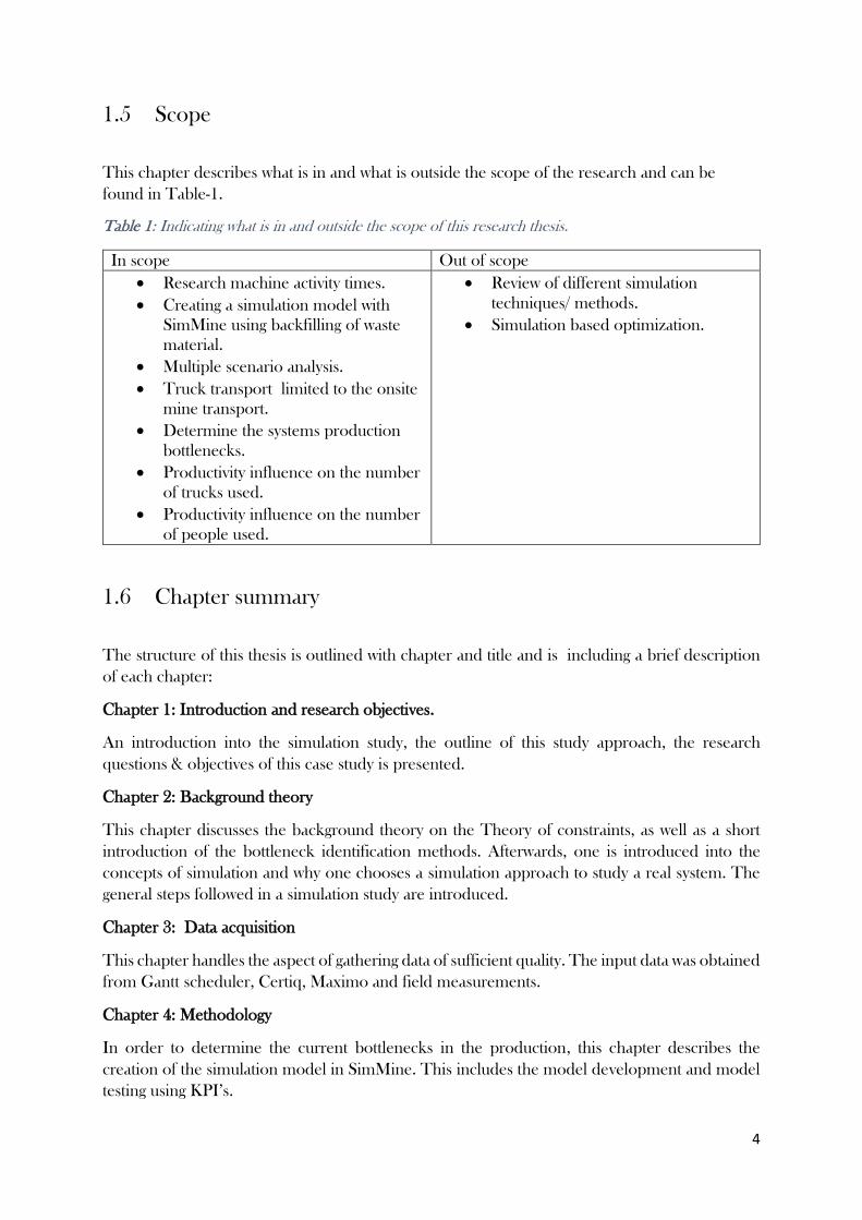
1.5 Scope

This chapter describes what is in and what is outside the scope of the research and can be

found in Table-1.

Table 1: Indicating what is in and outside the scope of this research thesis.

In scope Out of scope

• Research machine activity times.

• Creating a simulation model with

SimMine using backfilling of waste

material.

• Multiple scenario analysis.

• Truck transport limited to the onsite

mine transport.

• Determine the systems production

bottlenecks.

• Productivity influence on the number

of trucks used.

• Productivity influence on the number

of people used.

• Review of different simulation

techniques/ methods.

• Simulation based optimization.

1.6 Chapter summary

The structure of this thesis is outlined with chapter and title and is including a brief description

of each chapter:

Chapter 1: Introduction and research objectives.

An introduction into the simulation study, the outline of this study approach, the research

questions & objectives of this case study is presented.

Chapter 2: Background theory

This chapter discusses the background theory on the Theory of constraints, as well as a short

introduction of the bottleneck identification methods. Afterwards, one is introduced into the

concepts of simulation and why one chooses a simulation approach to study a real system. The

general steps followed in a simulation study are introduced.

Chapter 3: Data acquisition

This chapter handles the aspect of gathering data of sufficient quality. The input data was obtained

from Gantt scheduler, Certiq, Maximo and field measurements.

Chapter 4: Methodology

In order to determine the current bottlenecks in the production, this chapter describes the

creation of the simulation model in SimMine. This includes the model development and model

testing using KPI’s.

5

Chapter 5: Results

The first part of the results handles the result of the PIP bottleneck method. The bottlenecks are

indicted for the mining situation of 2019 and when additional trucks are added into the

simulation. The cycle time and waiting times are discussed for the different simulated scenarios.

Then the production results are presented, and the chapter ends with a financial analysis of the

simulated scenarios.

Chapter 6: Discussion

A review on possible assumptions that can influence the outcome of the simulation study.

Chapter 7: Conclusion

The conclusion starts with a recap of the main questions and the answers before coming to the

main conclusion.

Chapter 8: Further research

This chapter provides the potential improvements and discusses the further research topics.

6

2 Background theory This chapter discusses the background theory on the Theory of constraints, as well as a short

introduction of the bottleneck identification methods. Afterwards, one is introduced into the

concepts of simulation and why one chooses a simulation approach to study a real system. The

general steps followed in a simulation study are introduced.

2.1 Theory of Constraints Nowadays, companies struggle more to survive in global competition. It becomes more critical

for companies to focus on the understanding of their process structure, being in the production

or service sector. The theory of constraints becomes a critical theory focussing on finding the

weakest ring in the chain of production. This theory concentrates on the weakest points, which

can be the bottleneck for the entire company. Also, the relationship between the bottleneck is

being determined. The TOC is based on the idea that every system has at least one bottleneck

defined in a way that it impedes the system reaching the performance levels for its purpose

(Goldratt, 1990).

In the 1980s Goldratt focused the studies on the optimized production technology. With the

book “The Goal” from 1984, research about the TOC was increased, and a so-called “ drum-

buffer-rope” concept was developed. Studies focused more and more on the TOC thinking

process as an important tool for project management. After 40 years it is still one of the greatest

strategies for companies (Simsit, 2014).

The capacity management in operations is divided into long term and short term capacity issues.

TOC defers consideration of long term capacity issues via a four steps continuous framework

(Mahesh, 2008):

1. Identifying the constraints, i.e. a process that has insufficient capacity to meet the demand

of the system; (e.g. machines, demand, people). Prioritize the constraints according to the

impact they have on the goal of the organization;

2. Exploiting the constraint’s existing capacity: With a physical constraint, the objective

should be to make the constraint as effective as possible;

3. Subordinating the rest of the system to constraint capacity before adding additional

capacity. Every other component in the system should be changed to support the

maximum effectiveness of the constraint.

4. Elevating the constraint, i.e. adding additional capacity; When the performance of the

constraint is improved, this will lead to an overall system performance improvement.

TOC does not address medium-term issues; the firm must live with capacity constraints caused

by plant and significant equipment. Also, TOC is a continuous process (Figure-1), and no solution

will be correct for all time and every situation. It is essential to recognize this for an organization,

that when the business environment changes, the business policy has to account for these changes

(Rahman, 2002).

Figure 1: Schematic overview of TOC thinking process framework.

7

2.1.1 Production Bottlenecks

The performance of a mining system, like throughput, cycle time, delay, etc., are affected by

machine capacities and resources available in the mining system. Some capacities may affect

system performance more than others. The limitations in a system can be traced back to

limitations in machines or resources; one could also refer to this as a bottleneck. In order to

improve system performance, it is necessary to improve the bottlenecks. Bottlenecks can be

identified using different identification methods. This identification is not always straightforward

since many factors, such as machine capacity and resource capacity, contribute to bottlenecks.

In large systems, the variability is a crucial characteristic for evaluating the performance of that

system. With small variability in bottlenecks, a system can generate high production variability

(Wang, 2005). According to one of the definitions: a bottleneck is an element of a production

process, where every resource used to maximise production, is used for 100%. This percentage

of production capacity of a given workstation is a considerable threat to the effectiveness of the

production process. When the workstation is the bottleneck, this is characterised by the highest

level of exploitation, and this also means the highest risk of failure. (Kikolski, 2016) So,

bottlenecks have a negative effect on the efficiency of the production systems, material flow and

workstations.

When one considers a simplified process consisting of five steps, as shown in Figure-2, any step

in the process can be the bottleneck. In Figure-2 the bottleneck is indicated as workstation 3.

Imagine that each workstation has a cycle time for each step, while the individual sum of the steps

may take for instance 50 minutes, it is not unusual to think of a total cycle time for the process to

increase to multiple hours. Suppose that the time to fulfil a typical application takes 10 hours, the

challenge for the operation manager is to reduce the end-to-end time. Wait times can be

introduced at each step because of inventory waiting times, resulting in delays in the entire

process.

Figure 2 : Representation of a bottleneck in a simplified five step production system reproduced after (Kikolski, 2016). The bottleneck is indicated at workstation 3, resulting in delays in the entire process.

There is a variety of bottleneck detection methods to identify the bottleneck and reduce the

waiting time. A summary of several methods from the last decades is provided in Figure-3. In this

thesis, not all methods are reviewed, and for bottleneck detection, the PIP method is used. The

bottleneck detection processes are based on the observed or simulation time stamp data. The

diversity of the systems of a production network can make it difficult to accurately recognise the

bottlenecks in large systems (Wang, 2005).

8

Companies frequently focus on vertical improvements, such as speeding up one step in a process,

without the understanding of the impact on the horizontal value-added process. In the example

of Figure-2, one would focus on improving the waiting time of workstation 2, apart from creating

a suboptimal process, it has practically no impact on the end-to-end efficiency of the process.

Figure 3: Schematic overview of bottleneck detection methods from the last decades (Wang, 2005). The methods developed are all based on measuring the Average Waiting Time, Average Workload and Average Active Duration. In the top row the PIP based detection methods are presented.

2.1.2 Bottleneck detection using Performance In Processing method

The bottleneck can be detected by using analytical methods and simulation-based methods.

Developing analytical closed-form solutions for thorny stems is difficult. Compared to

analytical methods, discrete event simulation may be used to understand complex layout. (Li,

2008). The bottleneck detection methods process the observed factory data or simulation data.

The systems diversity of the production network can make it difficult to accurately recognise

the bottlenecks in large systems (Wang, 2005). There is no clear consensus on the type of

bottleneck definitions. The main bottleneck types, according to Lima, can be classified into

three categories (Lima, 2008):

• Simple Bottlenecks: there is only one bottleneck machine during the entire period

considered.

• Multiple Bottlenecks: there are more than one bottlenecks, but these are fixed for the

whole of the period considered.

• Shifting bottleneck: the bottleneck is instantly shifting between one station to the other.

According to (Wang, 2005) definitions are classified into two primary categories: performance

in processing (PIP) and sensitivity based definitions. In PIP average waiting time and capacity

are essential results. Evaluating PIP using simulation is an important bottleneck detection

method. Within the PIP-method, there are different branches of measuring: the average waiting

time, average workload and average active duration.

The theory of constraints suggest that all improvement efforts should be focused on the

bottleneck, because an hour lost on the bottleneck is an hour lost on the entire end-to-end

process, according to Goldratt (1990) there are three decisions to make while dealing with these

constraints:

9

1. Decide what to change;

2. Decide what to change to;

3. Decide how to cause the change.

Efforts to reduce the cycle time should be focused on alleviating the bottleneck, so the next

question becomes “decide what to change”. This second step, while dealing with constraints, is

meant to search for a solution to the core problem; therefore, it is essential to develop practical

and straightforward solutions. Different tools are described in the literature, including work

standardisation, elimination of non-value-added activities and job balancing. The last question

for an organisation to answer is “how to cause the change”, where one decides how to overcome

the obstacles (Rahman, 2002).

The changes are implemented to increase the efficiency in the system, but implementation

brings undesired effects. Therefore according to Noreen (1995) and Rahman (2002), it is

essential to:

• Identify the consequences when implementing the change.

• Determine possible causes of these consequences.

• Develop causal relationships between causes and effects.

2.1.3 Measuring waiting time

When measuring the waiting time, the machine with the longest waiting time is considered to be

the bottleneck. Recognising that the machine with the longest waiting time is the bottleneck was

first described by (Law & Kelton, 1991).

This can be described as in Equation (1), where Wi is the average waiting time of products of the

ith machine. For systems, without buffers or limited buffers, this way of analysing is not a suitable

method. When several machines have the same waiting time, this method cannot determine the

unique bottleneck. This approach analysis only the processing machines of the manufacturing

system (Wang, 2005).

𝑩 = {𝒊|𝑾𝒊 = 𝐦𝐚𝐱(𝑾𝟏,𝑾𝟐, … ,𝑾𝒏)}

(1)

2.1.4 Measuring workload

The machine with the larges idle ratio is considered to be the bottleneck according to (Knessl,

1998). This is obtained by using the average utilization measuring method from equation (2).

Where, pi is the utilization of the ith machine expressed as 𝜌𝑖 =λ𝑖𝜇𝑖⁄ . Where λ𝑖 and 𝜇𝑖 are

the arriving rate and service rate of the ith machine.

𝑩 = {𝒊|𝝆𝒊 = 𝐦𝐚𝐱(𝝆𝟏, 𝝆𝟐, … , 𝝆𝒏)}

(2)

When multiple machines may have a similar workload, the difference in utilisation may be

minimal. This analysing may result in numerous bottlenecks. Also, because workload

measurements may have errors due to the random variation of the data, it can be hard to decide

which entity is the bottleneck.

10

2.1.5 Measuring the average active duration

This method is based on the duration when a machine is active without interruption. Machines

can be grouped in either active states or inactive states. A state is active whenever the machine

causes other machines to wait. A state is inactive when it is waiting on the completion of another

task. This bottleneck detection method compares the duration of the active periods of the

different machines. The analysis can be based on simulation or historical data. (Roser, Nakano,

& Tanaka, 2001). A simulation approach was proposed using the average active duration method

by (Tamilselvan, 2010). The machine is considered the bottleneck when in the active state it has

the longest processing time among all other machines in the system.

Figure 4: Schematic overview of the Inactive and Active Period of a machine. Where the average of the active period is measured for different machines in order to determine the bottleneck with the longest average active duration.

11

2.2 Simulation Theory

A model is a representation of a system of interest, that is constructed and works as an imitation

of the system of interest. The model is similar to the system that it represents, but then in a simpler

manner, because a good model is a trade-off between realism and simplicity. In general, a model

used for a simulation study is a mathematical model developed using simulation software. The

model is used to do experiments since it is generally too expensive to apply changes in the real

system, and therefore experimental changes are applied to the model it represents (Maria, 1997).

A simulation is the imitation of the operation of a real-world process or system operation over

time. Simulation is used to analyse the behaviour of a system and ask what-if questions about the

real system (Banks, 1998). The simulation is used to reduce the chances of failure, or to remove

unforeseen bottlenecks (Maria, 1997). A set of data inputs are entered into the model. The model

is run for a while, and afterwards, the output can report the performance of the system. The

experiments continue by asking “what if” questions by changing the inputs and predicting the

outcome. There are reasons why simulations would be preferred to mathematical programming

or heuristic methods such as l, dynamic programming, linear programming, simulated annealing

& genetic algorithms, because simulations can model the variability and the effect the variability

has on the system (Robinson & Higton,1995).

By a study from Robinson and Higton (1995) “static” analysis was compared to a simulation

analysis, applied to a manufacturing plant, and the simulation showed the variability, resulting

mainly from equipment failures, in detail. The “static” analysis predicted that each design

would reach the throughput required; the simulation showed that the “static” analysis was not

satisfactory (Robinson & Higston, 1995). Using simulation also limits the number of

assumptions. It creates transparency because it is more intuitive, and an animated display of the

system can be made, providing more confidence in the model (Robinson, 2004).

Instead of using a simulation model, experiments can be carried out in the real world system.

There are some advantages why simulation is preferred instead of doing direct experimentation.

With the benefits also several problems arise when using a simulation approach.

Experimentation in the real system is costly. It is expensive to disturb the daily production to

try out new ideas. With implementing the changes, the system has to shut down and might

worsen the operations performance. Simulation changes can be implemented and altered in the

model without interruption of the real system. It can be time-consuming to experiment with a

Figure 5: Using the Simulation Model for an experimentation approach reproduced after (Robinson & Higton, 1995). Sometimes preferred over heuristic methods, because simulations are able to model the variability and effect of the variability.

12

real system. Depending on the size of the model, and the computational speed of the computer,

a simulation can run many times faster than a real-time system and results can be obtained

within minutes. Another advantage is that results can be obtained over a very long time frame

within production. It is useful to control the condition under which the experiments are

performed so that direct comparison is possible. The conditions under which an experiment is

performed can be generated again and again with a simulation model. When no real system

exists, the only alternative is to develop a model (Robinson, 2004).

Next to the advantages, there are some disadvantages to a simulation study. Simulation software

is not cheap, and the cost of model development can make it expensive, especially when one

needs to employ consultants. It is also a time-consuming approach. A simulation model requires

a significant amount of data, which is not always available, and data analysis is required before

using it as input for the simulation. Simulation is more than the development of a computer

program or the usage of a software package. It requires skills in conceptual modelling,

validation and statistics, as well as skills in working with people and project management. When

obtaining results from the simulation, one must consider the validity of the underlying model

and assumptions and simplifications (Robinson, 2004).

2.2.1 System Model Classifications

A system is defined to be a collection of entities, e.g. machines or people, that interact logically.

A system can be discrete or continuous. A discrete system is where the state variables change

instantaneously at separated points in time, and a continuous system changes continuously in

respect with time. In most systems, there is the need to study them to gain inside in the

relationship between different components or predict the performance under new circumstances.

Figure-6, shows multiple ways to study a system, and Figure- 7 reviews the types of system models

(Law & Kelton, 1991).

Systems can be studied in multiple ways. One can experiment with the existing system or with the

model (Figure-6). It is rarely possible to change the physical system to let it operate under new

conditions since it is simply too costly, therefore one would use a model. When working with the

model of a system, one can choose between a physical model or a mathematical model. Examples

of physical models are cars in wind tunnels or tabletop scale models. But the majority are

mathematical models, representing a system in logic and quantitative relationship where one can

manipulate the model to see how it reacts. The mathematical model can be then expressed as an

analytical solution or a simulation. When a mathematical model is built, one must determine

how the model can be examined in order to see how it can answer the questions of interests. It is

desired to study a model in an analytical way; many systems are highly complex, providing no

13

analytical solution. In this case, the model is studied using simulation, changing the inputs in

question to see how they affect the output measures of performance.

Figure 6: Multiple ways to study a system (reproduced after Law & Kelton, 1991)

Simulation models can be classified into three different fields. The first class being deterministic

or stochastic simulation models as seen in Figure-7. When a simulation model doesn’t contain

any random components, it is deterministic, and this can be a system of differential equations. In

stochastic simulation models, the output itself is random; therefore, it is treated as an estimate of

the actual characteristics of the model. The second class consist of static or dynamic simulation

models, where a static model is a representation of a system at a particular time, like Monte Carlo

models. The other type of model is a dynamic simulation model representing a system changing

over time. The last class would be continuous or discrete simulation models. How a system can

be described using a discrete or a continuous model is depended on the study objective. Where

one would like to know the traffic flow of individual cars, one would create a discrete model.

When the flow of vehicles is to be treated as a single thing, then it can be described by differential

equations (Gosavi, 2014).

Figure 7: Types of system models (reproduced after Kelton & Law, 2000). Discrete-event-simulation used for this study, is a stochastic continuous system model.

14

2.2.2 Discrete event simulation

In this thesis, the focus lies on creating a discrete event stochastic model, because of the size and

complexity of an underground cut and fill mining operation, where one would like to know the

individual traffic flow of the mining machines. Formulating an objective function can be difficult

and complicated because of the stochastic setting (Gosavi, 2014). In this case, due to a large

number of random variables in the system, it can hardly be expressed in a closed-form.

Therefore, the outputs can be generated using different parameters inputs into a discrete event

simulation model. The system itself is complex and also depends on a lot of complex inputs,

having randomness and uncertainty that needs to be considered in the model.

In a discrete-event system, one or more phenomena of interest change from their state or value

in a discrete point in time. In generally a discrete-event exists out of seven concepts: work,

resources, routing, buffers, scheduling, sequencing and performance. With work; items, jobs or

customers are denoted. Resources include the machines, equipment or human resources that

can provide a service to the item or costumer. For each unit, a route is applied in order to

delineate the collection of the required service and the order of the service. Buffers are waiting

rooms, where an item has to wait for the service they receive, they can have a limited or unlimited

capacity. The scheduling denotes the number of resources available, and the sequencing

characterises the order in which the resource provides service to their work. This is also called

the queuing discipline (Fishman, 2001).

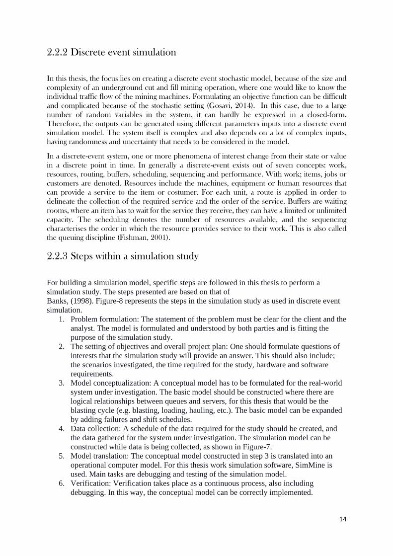
2.2.3 Steps within a simulation study

For building a simulation model, specific steps are followed in this thesis to perform a

simulation study. The steps presented are based on that of

Banks, (1998). Figure-8 represents the steps in the simulation study as used in discrete event

simulation.

1. Problem formulation: The statement of the problem must be clear for the client and the

analyst. The model is formulated and understood by both parties and is fitting the

purpose of the simulation study.

2. The setting of objectives and overall project plan: One should formulate questions of

interests that the simulation study will provide an answer. This should also include;

the scenarios investigated, the time required for the study, hardware and software

requirements.

3. Model conceptualization: A conceptual model has to be formulated for the real-world

system under investigation. The basic model should be constructed where there are

logical relationships between queues and servers, for this thesis that would be the

blasting cycle (e.g. blasting, loading, hauling, etc.). The basic model can be expanded

by adding failures and shift schedules.

4. Data collection: A schedule of the data required for the study should be created, and

the data gathered for the system under investigation. The simulation model can be

constructed while data is being collected, as shown in Figure-7.

5. Model translation: The conceptual model constructed in step 3 is translated into an

operational computer model. For this thesis work simulation software, SimMine is

used. Main tasks are debugging and testing of the simulation model.

6. Verification: Verification takes place as a continuous process, also including

debugging. In this way, the conceptual model can be correctly implemented.

15

7. Validation: This is the stage where one determines if the model represents the real

system in enough detail. The ideal way to validate is to compare the output of the real

system with the computer model. There are multiple ways to validate a model.

8. Experimental design: For each scenario that is to be studied, the length of the

simulation run, the number of runs, and the manner of initialization should be

determined.

9. Production runs & analysis: These are used to measure the performance of each

scenario that is being simulated.

10. More runs: One should determine if more runs are needed or additional scenarios are

required for the analysis.

11. Documentation & reporting: Documentation is important when the model is used by

the same or different analyst. Also, when one wants to make changes in the model

documentation can facilitate this.

12. Implementation: Likelihood of performance is increased when the client is involved

throughout the simulation studies.

Figure 8: Steps in a discrete-event simulation study (reproduced after Banks,1998).

16

2.2.4 Verification and validation

Testing of the simulation model is an essential element of a simulation study. A model is never

100% accurate and is also not created to be completely accurate, but a simplified model for

exploring reality (Pidd, 2003). Without verification and validation of the model, there is no

confidence in the study results. Verification and validation is used to ensure that the model is

sufficiently accurate (Banks, 1998).

• Verification: This is the process of ensuring that the model design has been transformed

into a computer model with sufficient accuracy.

• Validation: The two key concept in validation are: that the model should have sufficient

accuracy and is built for a specific purpose. Validity is a binary decision, a model is or

isn’t sufficiently accurate for its purpose.

What should be noticed is that validation and verification are not done once, but is a continuous

process being performed through the period of the simulation study. The modelling part is an

iterative process, just as the validation and verification. Each part of the cycle, as shown in Figure-

9, is likely to be revised, as the understanding of the problem changes. The whole procedure is a

trial-and-error process.

There are various forms of validation, but the main validation methods used in this thesis are

represented in Figure-9, adapted from (Landry,1983). The different types of validation:

conceptual model validation, verification, experimentation validation and solution validation,

were more comfortable to do because a specialized simulation software was used. Data validation,

determining that the use for the model are sufficiently accurate for the purpose. With the

experimental validation is meant that the testing procedures adopted are providing results that

are sufficiently accurate. The solution validation determines that the result obtained from the

model are compared with the solutions of the real world (Robinson, 2004).

Figure 9: Simulation Model Verification and Validation in a Simulation Study adapted from (Landry, 1983)

17

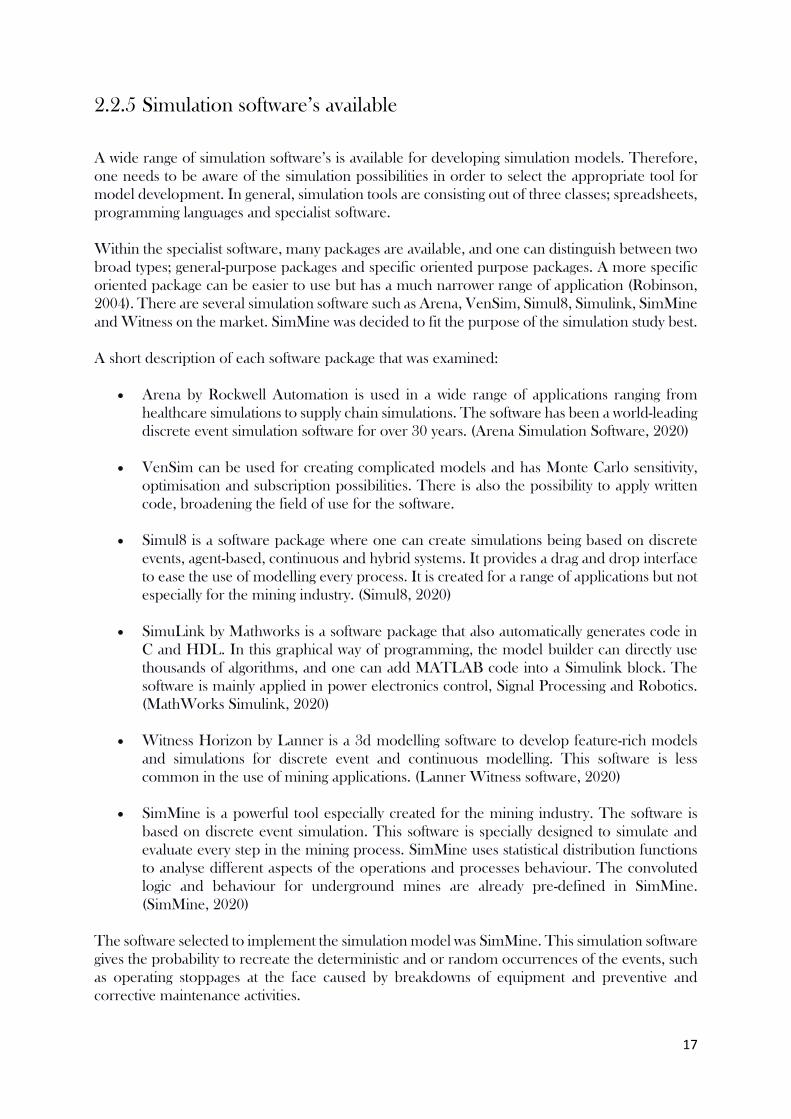
2.2.5 Simulation software’s available

A wide range of simulation software’s is available for developing simulation models. Therefore,

one needs to be aware of the simulation possibilities in order to select the appropriate tool for

model development. In general, simulation tools are consisting out of three classes; spreadsheets,

programming languages and specialist software.

Within the specialist software, many packages are available, and one can distinguish between two

broad types; general-purpose packages and specific oriented purpose packages. A more specific

oriented package can be easier to use but has a much narrower range of application (Robinson,

2004). There are several simulation software such as Arena, VenSim, Simul8, Simulink, SimMine

and Witness on the market. SimMine was decided to fit the purpose of the simulation study best.

A short description of each software package that was examined:

• Arena by Rockwell Automation is used in a wide range of applications ranging from

healthcare simulations to supply chain simulations. The software has been a world-leading

discrete event simulation software for over 30 years. (Arena Simulation Software, 2020)

• VenSim can be used for creating complicated models and has Monte Carlo sensitivity,

optimisation and subscription possibilities. There is also the possibility to apply written

code, broadening the field of use for the software.

• Simul8 is a software package where one can create simulations being based on discrete

events, agent-based, continuous and hybrid systems. It provides a drag and drop interface

to ease the use of modelling every process. It is created for a range of applications but not

especially for the mining industry. (Simul8, 2020)

• SimuLink by Mathworks is a software package that also automatically generates code in

C and HDL. In this graphical way of programming, the model builder can directly use

thousands of algorithms, and one can add MATLAB code into a Simulink block. The

software is mainly applied in power electronics control, Signal Processing and Robotics.

(MathWorks Simulink, 2020)

• Witness Horizon by Lanner is a 3d modelling software to develop feature-rich models

and simulations for discrete event and continuous modelling. This software is less

common in the use of mining applications. (Lanner Witness software, 2020)

• SimMine is a powerful tool especially created for the mining industry. The software is

based on discrete event simulation. This software is specially designed to simulate and

evaluate every step in the mining process. SimMine uses statistical distribution functions

to analyse different aspects of the operations and processes behaviour. The convoluted

logic and behaviour for underground mines are already pre-defined in SimMine.

(SimMine, 2020)

The software selected to implement the simulation model was SimMine. This simulation software

gives the probability to recreate the deterministic and or random occurrences of the events, such

as operating stoppages at the face caused by breakdowns of equipment and preventive and

corrective maintenance activities.

18

2.2.6 Application in mining

The mining industry is using computer simulation models already since the 1960s to investigate

production lines. Properly working simulation models can help when making critical decisions

by simulating the implemented changes in the simulation model before implementing them in

the real system. Traditional methods are not sufficient to solve complex mining problems due to

the complexity and magnitude of the system; therefore, the constant development of tools and

methods are being developed and improved.

The theory of constraints has been popular since the 1980s in manufacturing industries. The

TOC has been successfully implemented in assembly production lines but has not become so

popular in mining industries. According to Ferencikova (2012), the Theory of Constraints is more

difficult to apply in complicated production systems, but can result in a better production

planning. When looking for past research, only a few sources were found describing TOC

management for the mining industry, the following examples are:

• Bloss (2009) used the Theory of Constraints to remove the bottleneck of an underground

mine operation,. This resulted in an 18% throughput improvement over a time period 24

months. This was considered an empirical approach and used a waterfall chart. I this way

capacity is compared with actual production to identify the bottleneck in the system.

• For a coal mine in China a dynamic optimization model was created by Hong-Jun et al.

(2009) to solve a supply chain problem.

• Phillis (2011) used Critical Chain Project Management (CCPM), this is a TOC project

management approach. TOC was applied to improve the stoping performance in an

underground platinum mine.

• Simulation was used by Miwa & Takakuwa (2011) to indicate the constraint of a material

handling system of an underground coal mine.

• Biswal (2012) detected the bottleneck of an iron ore beneficiation plant using a simulation

model.

• Khan (2013) used the theory of constrains and a discrete event simulation to identify the

the bottlenecks in a mine in Vale Canada.

• Kahraman (2015) developed a methodology for creating a Bottleneck Identification

Model (BIM) for mine management.

• Heerden (2015) used TOC and time to determine the bottleneck in an underground coal

mine that used shuttle cars and continuous miners.

• Baafi et al. (2015) applied the TOC to the pillar development cycle of an underground

coal mine to determine the constraints of the system.

• Sobiyi K (2017) used the Lonmin platinum mine to implement the Theory of constraints

to determine its bottlenecks.

19

3 Data acquisition

3.1 Boliden Area

The mining operations in Boliden started when

gold was discovered at Fågelmyran in Västerbotten

county in 1924. The first ore was produced in 1926

and the Rönnskär smelter started its operations in

1930. Currently, the Boliden area operations exists

out of three underground mines all delivering ore

to a common concentrator in Boliden. The

concentrate is trucked to the port of Rönnskär to

be treated by the smelter or shipped out to

costumers from the port (New Boliden ).

3.1.1 Kankberg Mine

The mine under study is an underground cut and fill mine located approximately 10 km west of

the Boliden processing plant. The mines primary product is ore containing gold and tellurium

from a deposit hosted by volcanic and volcaniclastic rock types. The Au deposit is located at a

depth ranging from 200-700 m and is situated below the former Åkulla Östra open pit mine.

Figure-11 is a simplified map to show the approximate location of the deposit in relation to the

three historic open pit locations, current underground orebody, decline access ramp and

Kankberg mine offices. The map coordinate system is SWEREF99 TM.

Figure 10: Boliden mining operations in

Västerbotten county with three underground

mines Kristineberg, Renström & Kankberg. The

processing plant is located in Boliden and smelter

in Rönnskär (New Boliden ).

Figure 11: Simplified map of 2 km x 2.5 km area

showing the Kankberg mining operation, with

orebody outline, access and land rights (New

Boliden).

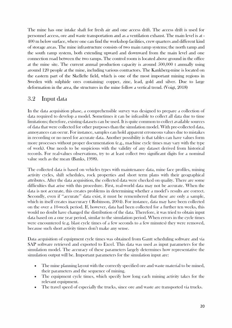
20

The mine has one intake shaft for fresh air and one access drift. The access drift is used for

personnel access, ore and waste transportation and as a ventilation exhaust. The main level is at -

400 m below surface, where one can find the workshop facilities, crew quarters and different kind

of storage areas. The mine infrastructure consists of two main ramp systems; the north ramp and

the south ramp system, both extending upward and downward from the main level and one

connection road between the two ramps. The control room is located above ground in the office

at the mine site. The current annual production capacity is around 500,000 t annually using

around 120 people at the mine, including various contractors. The Kankberg-mine is located on

the eastern part of the Skellefte field, which is one of the most important mining regions in

Sweden with sulphide ores containing: copper, zinc, lead, gold and silver. Due to large

deformation in the area, the structures in the mine follow a vertical trend. (Voigt, 2018)

3.2 Input data

In the data acquisition phase, a comprehensible survey was designed to prepare a collection of

data required to develop a model. Sometimes it can be infeasible to collect all data due to time

limitations; therefore, existing datasets can be used. It is quite common to collect available sources

of data that were collected for other purposes than the simulation model. With pre-collected data,

annoyances can occur. For instance, samples can hold apparent erroneous values due to mistakes

in recording or no need for accurate data. Another possibility is that tables can have values form

more processes without proper documentation (e.g., machine cycle times may vary with the type

of work). One needs to be suspicious with the validity of any dataset derived from historical

records. For real-values observations, try to at least collect two significant digits for a nominal

value such as the mean (Banks, 1998).

The collected data is based on vehicles types with maintenance data, mine face profiles, mining

activity cycles, shift schedules, rock properties and short term plans with their geographical

attributes. After the data acquisition, the collected data were checked on quality. There are some

difficulties that arise with this procedure. First, real-world data may not be accurate. When the

data is not accurate, this creates problems in determining whether a model’s results are correct.

Secondly, even if ‘‘accurate’’ data exist, it must be remembered that these are only a sample,

which in itself creates inaccuracy ( Robinson, 2004). For instance, data may have been collected

on the over a 10-week period. If, however, data had been collected for a further ten weeks, this

would no doubt have changed the distribution of the data. Therefore, it was tried to obtain input

data based on a one year period, similar to the simulation period. When errors in the cycle times

were encountered (e.g. blast cycle times of a few seconds to a few minutes) they were removed,

because such short activity times don’t make any sense.

Data acquisition of equipment cycle times was obtained from Gantt scheduling software and via

SAP software retrieved and exported to Excel. This data was used as input parameters for the

simulation model. The accuracy of these parameters largely determines how representative the

simulation output will be. Important parameters for the simulation input are:

• The mine planning layout with the correctly specified ore and waste material to be mined,

their parameters and the sequence of mining.

• The equipment cycle times, which specify how long each mining activity takes for the

relevant equipment.

• The travel speed of especially the trucks, since ore and waste are transported via trucks.

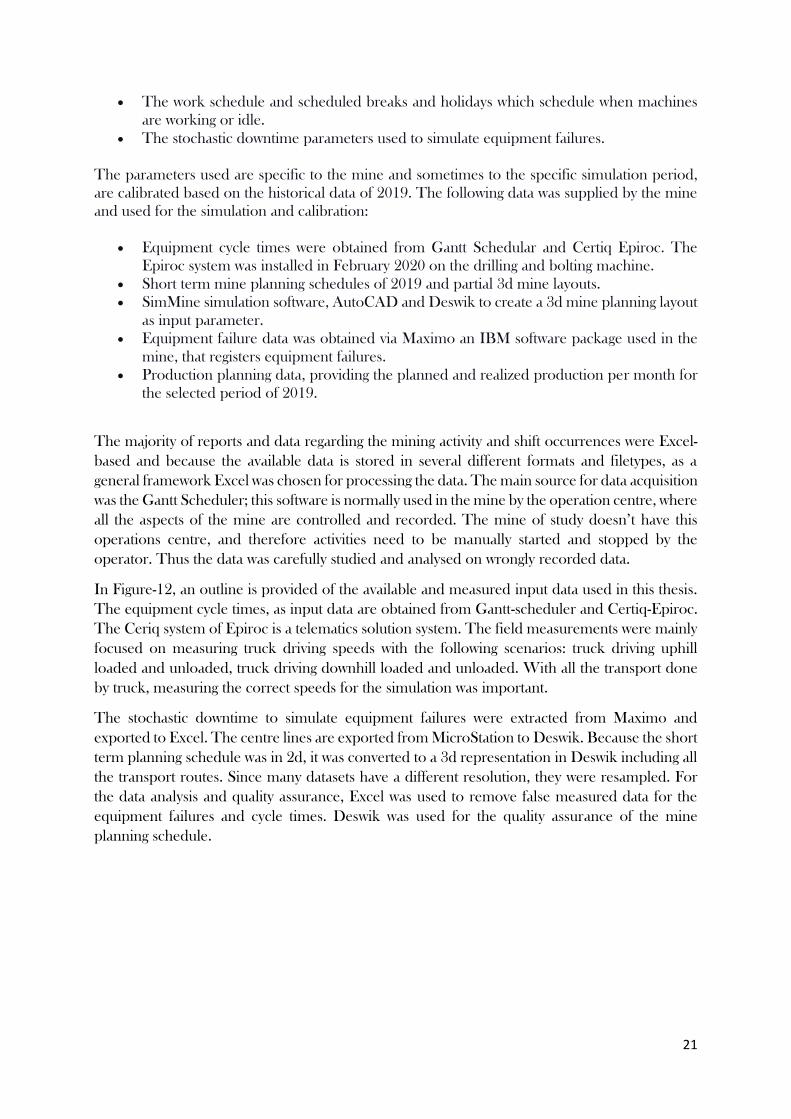
21

• The work schedule and scheduled breaks and holidays which schedule when machines

are working or idle.

• The stochastic downtime parameters used to simulate equipment failures.

The parameters used are specific to the mine and sometimes to the specific simulation period,

are calibrated based on the historical data of 2019. The following data was supplied by the mine

and used for the simulation and calibration:

• Equipment cycle times were obtained from Gantt Schedular and Certiq Epiroc. The

Epiroc system was installed in February 2020 on the drilling and bolting machine.

• Short term mine planning schedules of 2019 and partial 3d mine layouts.

• SimMine simulation software, AutoCAD and Deswik to create a 3d mine planning layout

as input parameter.

• Equipment failure data was obtained via Maximo an IBM software package used in the

mine, that registers equipment failures.

• Production planning data, providing the planned and realized production per month for

the selected period of 2019.

The majority of reports and data regarding the mining activity and shift occurrences were Excel-

based and because the available data is stored in several different formats and filetypes, as a

general framework Excel was chosen for processing the data. The main source for data acquisition

was the Gantt Scheduler; this software is normally used in the mine by the operation centre, where

all the aspects of the mine are controlled and recorded. The mine of study doesn’t have this

operations centre, and therefore activities need to be manually started and stopped by the

operator. Thus the data was carefully studied and analysed on wrongly recorded data.

In Figure-12, an outline is provided of the available and measured input data used in this thesis.

The equipment cycle times, as input data are obtained from Gantt-scheduler and Certiq-Epiroc.

The Ceriq system of Epiroc is a telematics solution system. The field measurements were mainly

focused on measuring truck driving speeds with the following scenarios: truck driving uphill

loaded and unloaded, truck driving downhill loaded and unloaded. With all the transport done

by truck, measuring the correct speeds for the simulation was important.

The stochastic downtime to simulate equipment failures were extracted from Maximo and

exported to Excel. The centre lines are exported from MicroStation to Deswik. Because the short

term planning schedule was in 2d, it was converted to a 3d representation in Deswik including all

the transport routes. Since many datasets have a different resolution, they were resampled. For

the data analysis and quality assurance, Excel was used to remove false measured data for the

equipment failures and cycle times. Deswik was used for the quality assurance of the mine

planning schedule.

22

3.3 Data processing of time studies

To increase the balance and efficiency of the mining operation, a time study was carried out to

find the durations of the task. The duration to complete a work task depends on a lot of factors

such as the type of work to be done, the operator, day shift/ night shift etc. Therefore to determine

the approximate real process time of the job, a time study was performed were measurements

were recorded in minutes and seconds. The collected activity times were tested for distribution

fit and goodness of fit.

It was sometimes difficult to produce a reasonable histogram because of limited data

measurements. When there are less than 50 data points, it is likely that no standard distribution

will provide an outstanding data fit. When one becomes familiar with the data, the following steps

are suggested by (Banks, 1998):

1. Use the knowledge of the source to determine the definite limits on the values of the data.

Determine which values are absolutely impossible and therefore, undesirable to use for

the simulation.

2. Try to fit multiple distributions to the data.

3. Use a set of criteria to rank how good the distribution fits the observed data.

4. If any data is inconsistent with the assumed range for the source of randomness, rule them

out.

5. Be reasonable in determining the best-fitted distributions as a representation for the data.

6. If the best of the fitted distributions provide a reasonable representation of the data, use

it in the simulation. Otherwise use an empirical distribution to represent the data directly.

When creating a histogram of the data, it is suggested to adjust the start point an interval with to

cover all the data. Some of the data may be well away from the rest and might be ignored during

the histogram construction. The most challenging step is to choose the appropriate interval width.

When the interval is too small, it will generate a ragged histogram, and when too large it produces

an over ragged block like a histogram.

The data collected from the Gantt Schedular and Certiq were used to analyse the equipment

cycle times. Distributions are classified as discrete when they produce a finite or countable

number of different values. It was chosen to work with nonnegative continuous distributions

taking on values in the range (x, ∞), where x can be 0 or another positive value because it is

unlikely to have negative equipment cycle times.

The cycle times collected from the database for 2019 was:

Figure 10: Outline of the input data, and used softwares for this simulation study. Figure 12: Outline of the input data, and used softwares for this simulation study.

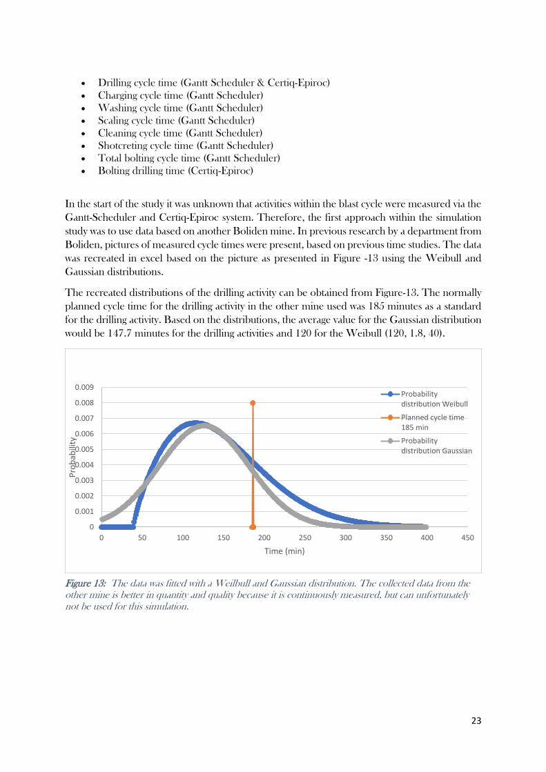
23

• Drilling cycle time (Gantt Scheduler & Certiq-Epiroc)

• Charging cycle time (Gantt Scheduler)

• Washing cycle time (Gantt Scheduler)

• Scaling cycle time (Gantt Scheduler)

• Cleaning cycle time (Gantt Scheduler)

• Shotcreting cycle time (Gantt Scheduler)

• Total bolting cycle time (Gantt Scheduler)

• Bolting drilling time (Certiq-Epiroc)

In the start of the study it was unknown that activities within the blast cycle were measured via the

Gantt-Scheduler and Certiq-Epiroc system. Therefore, the first approach within the simulation

study was to use data based on another Boliden mine. In previous research by a department from

Boliden, pictures of measured cycle times were present, based on previous time studies. The data

was recreated in excel based on the picture as presented in Figure -13 using the Weibull and

Gaussian distributions.

The recreated distributions of the drilling activity can be obtained from Figure-13. The normally

planned cycle time for the drilling activity in the other mine used was 185 minutes as a standard

for the drilling activity. Based on the distributions, the average value for the Gaussian distribution

would be 147.7 minutes for the drilling activities and 120 for the Weibull (120, 1.8, 40).

0

0.001

0.002

0.003

0.004

0.005

0.006

0.007

0.008

0.009

0 50 100 150 200 250 300 350 400 450

Pro

bab

ility

Time (min)

Probabilitydistribution Weibull

Planned cycle time185 min

Probabilitydistribution Gaussian

Figure 13: The data was fitted with a Weilbull and Gaussian distribution. The collected data from the other mine is better in quantity and quality because it is continuously measured, but can unfortunately not be used for this simulation.

24

When it was discovered that activities of the blasting cycle were registered for the mine

understudy, all activity cycle times were analysed for this mine. Due to the number of

uncertainties in the cycle time parameters, and limited data measurements, a triangular

distribution was fitted to the measured data and chosen over a Normal- or Weibull distribution

to best represent the model input parameters as an empirical distribution to best represent the

data directly. Because the study is not focusing on comparing all the different types of

distributions, only the Gaussian and Triangular distributions are mentioned. Gaussian

distribution formula (Equation-4):

𝒈(𝒙) = 𝟏

𝝈√𝟐𝝅𝒆−

𝟏𝟐(𝒙−𝝁𝝈)𝟐

(4)

A Triangular distribution is a continuous probability distribution with a with a probability

density function shaped like a triangle. It is defined by the minimum value a, the maximum

value b, and the peak value c. A triangular distribution (Figure-14) has a defined upper and

lower limit so extreme unwanted values can be avoided. In addition, it is a good model for

skewed distributions with limited data.

Triangular distribution formula (Equation-5):

𝒇(𝒙|𝒂, 𝒃, 𝒄)

=

{

𝟎𝒇𝒐𝒓𝒙 < 𝒂,𝟐(𝒙 − 𝒂)

(𝒃 − 𝒂)(𝒄 − 𝒂)𝒇𝒐𝒓𝒂 ≤ 𝒙 ≤ 𝒄,

𝟐(𝒃 − 𝒙)

(𝒃 − 𝒂)(𝒃 − 𝒄)𝒇𝒐𝒓𝒄 < 𝒙 ≤ 𝒃,

𝟎𝒇𝒐𝒓𝒃 < 𝒙,

(5)

To estimate the relevant distribution fit of the data gathered, a histogram was created in Excel. In

this example, the drilling times are analysed. One of the first steps in the data analysis was

removing activity times over 436 minutes or 7.3 hours, because longer drilling durations are not

realistic for the mine. These long activity measurements present in the data were created because

activities were not stopped by the operators after they stopped working on the activity. Shortest

activity measurements in the drilling duration are 14 minutes. In the mining operation, short

drilling durations are possible, when small blasts of only a few holes take place to remove

additional ore from a pillar. Based on the input data a gaussian distribution was created and

placed over the histogram the Gaussian function didn’t fit the histogram properly because three

peaks in the frequency are present at around 50 minutes, 100 minutes and 145 minutes. When

Figure 14: Example of a Triangular distribution

25

decreasing the histogram bin sizes to a smaller size of width 10 as can be seen in Figure-15, it

becomes clear that two peaks occur with the highest frequency at 100 minutes and 145 minutes.

The mining operation uses different blast sizes and therefore different drill patterns for ore and

waste rock. This difference in face profile results in the peaks as can be seen in the data. The

waste drilling having the peak at around 100 minutes and ore drilling at around 145 minutes.

The drilling data had a mean of 172.17 minutes and a standard deviation of 95.94 minutes.

Because the data is so spread out for the drilling activity ranging from 14 minutes to 7.3 hours,

the also results in a high standard deviation. After this a first histogram was created of the drilling

data with bin size 50.

Based on the smaller bin size histogram, the triangular distribution was fitted as can be seen from

Figure-16. The peak value as fitted in the figure was determined to be 145.92 minutes. The shape

of this distribution, where the minimum, maximum, and peak values were selected, was based on

the data as presented in Figure-17. Because the drilling activity from Gantt-Scheduler was

measured manually, other datasets were also studied to recover the drilling cycle times. The

Epiroc-Certiq system was implemented on the drill rigs in February 2020 and started measuring

activity times from the beginning of March. This system is more reliable because activity times

are being measured automatically by the machine itself and doesn’t require a manual stop and

start. When looking at Figure-17, one can observe that the most occurring activity duration is

about 150 to 170 minutes, based on the Certiq data. Although this system had only data available

of 4 months, it is based on double the amount of data samples. This peak in the frequency

showing a duration of 150 min is similar to the second big peak in the Gantt Scheduler data

(Figure-15); therefore the distribution from was fitted with a triangular distribution as in Figure-

16. The input data of the Certiq system was studied to see what the most frequent time of the

drilling activity was as obtained in Figure-17. However, the triangular distribution was fitted to the

Gantt-Scheduler data, because this was data measured over 2019.

Figure 15 : Histogram showing the frequency distribution of the total drilling cycle time in minutes with a

mean of 172.17 and standard deviation of 95.94 and fitted Gaussian distribution. From this picture it

becomes clear that the distribution does not fit the data very well.

.

0.00 200.00 400.00 600.00 800.00 1000.00

00.00050.0010.00150.0020.00250.0030.00350.0040.0045

0

2

4

6

8

10

12

10

-20

50

-60

90

-10

0

13

0-1

40

17

0-1

80

21

0-2

20

25

0-2

60

29

0-3

00

33

0-3

40

38

0-3

90

43

0-4

40

47

0-4

80

52

0-5

30

56

0-5

70

61

0-6

20

65

0-6

60

69

0-4

00

74

0-7

50

78

0-7

90

82

0-8

30

86

0-8

70

90

0-9

10

94

0-9

50

98

0-9

90

10

20

-10

30

10

60

-10

70

11

00

-11

10

Astitel

Pro

bab

olit

y

Freq

uen

cy

Time(Minutes)

Frequency

Gaussian function

26

0 200 400 600 800 1000 1200

00.00050.0010.00150.0020.00250.0030.00350.0040.00450.005

0

2

4

6

8

10

121

0-2

0

50

-60

90

-10

0

13

0-1

40

17

0-1

80

21

0-2

20

25

0-2

60

29

0-3

00

33

0-3

40

38

0-3

90

43

0-4

40

47

0-4

80

52

0-5

30

56

0-5

70

61

0-6

20

65

0-6

60

69

0-4

00

74

0-7

50

78

0-7

90

82

0-8

30

86

0-8

70

90

0-9

10

94

0-9

50

98

0-9

90

10

20

-10

30

10

60

-10

70

11

00

-11

10

Pro

bab

ility

Freq

uen

cy

Time(Minutes)

Histogram

Triangular distribution

0

5

10

15

20

25

30

35

Freq

uen

cy

Time(Minutes)

Histogram

Figure 16: Triangular distribution fitted to the histogram of the drill activity time. The second peak around 145 minutes was chosen as the peak value taking into consideration the peak values of the Certiq data as presented in Figure-17.

Figure 17: Histogram distribution of Certiq rock drilling activity duration, showing peak values around 160 and 170 minutes.

27

3.3.1 Summary blast cycle time

Each activity was analysed in the same manner as the drilling data mentioned in Chapter-3.3

and can be found in Appendix-B. The activity times were fitted with a Gaussian distribution

and a triangular distribution. The activity time data for each activity of the blast cycle can be

found in Table-2 for the Gaussian distribution and in Table-3 for the triangular distribution.

The standard deviation for the blast cycle activities (Table-2) are high. The standard deviation

is a measure of the amount of dispersion of a set of values. A high standard deviation indicates

that the values are spread out over a wider range. There is a lot a variability in the length of

activity times in the mining operation resulting in this high standard deviation. The coefficient

of variation represents the ratio of the standard deviation to the mean, and is a measure of the

dispersion of the data series around the mean. Although the data is spread out, as a rule of thumb

one can apply that distributions with a coefficient of variation lower or equal to 1 are considered

low variance.

The triangular distribution is used as input data for the simulation, due to limited data

measurements. The cleaning activity had only eight activity measurements over 2019 and is

therefore not really analysed. As the input of the Cleaning activity, an average activity time of

11.02 minutes, with a minimum of 9.88 min and a maximum of 15.75 min was used because

this was in line with the field observations. The total bolting activity time derived from the

Gantt Scheduler had a mean of 325.15 minutes and a standard deviation of 275.72 minutes. The

bolting drilling time retrieved from Certiq had a mean of 104.25 minutes and a standard

deviation of 56.61. The bolting times were also fitted with a triangular distribution. With the

triangular distribution, the average bolting time was 287.60 minutes, and the bolting drilling

time 75.01 minutes and therefore, it took 15 minutes to drill one meter. The bolting time without

the drilling involved was, on average, 212.57 minutes; this translates to an average bolting

speed of 42.51 min per meter length (Table-4).

Table 2: Summary blast cycle activity times determined with the Gaussian distribution.

Activity Data

Source

Units Mean Standard

deviation

Coefficient of

variation

Drilling Gantt Minutes 172.17 95.94 0.56

Drilling Certiq Minutes 183.28 101.47 0.55

Charging Gantt Minutes 80.95 44.17 0.55

Washing Gantt Minutes 22.75 15.46 0.68

Loading Gantt Minutes 270.99 214.00 0.79

Scaling Gantt Minutes 105.89 75.45 0.71

Cleaning Gantt Minutes - - -

Shotcreting Gantt Minutes 66.22 44.45 0.67

Bolting Gantt Minutes 325.15 275.71 0.85

28

Bolting

drilling

Certic Minutes 104.25 56.61 0.54

Table 3: Summary activity times determined with a Triangular distribution.

Activity Units Minimum Maximum Mean

Drilling Min 14 436.85 145.92

Charging Min 6.42 169.60 70.70

Washing Min 1.05 70.80 13.07

Loading Min 13.55 691.55 156.42

Scaling Min 47.85 200.62 86.85

Face Scaling Min 5.8 57.67 31.20

Face Cleaning Min 9.88 15.75 11.02

Cleaning Min 30.48 71.48 43.22

Shotcreting Min 4.48 160.77 44.43

Bolting Min 46.42 485.18 287.58

Table 4: Bolting drilling times and Bolting times.

Units Min Mean Max

Bolting drill times Minutes 31.71 75.01 247.24

Min / length m 06.34 15.00 49.45

Bolting time Minutes 14.71 212.57 237.94

Min / length m 2.94 42.51 47.59

29

3.4 Equipment failure and downtime

In today’s ongoing 24/7 industry technical incidents resulting in downtime, and can come with

real consequences for the production. Therefore, it is important to track metrices such as:

downtime and how fast and effectively a repair team resolves the issue. Understanding the

metrices will eliminate the guess work and provide data to make informed decisions.

Industry most commonly tracked metrices are MTBF (mean time between failure) and MTTR

(mean time to repair). This data doesn’t provide any information about the type of failure and

how they are resolved, but it provides a benchmark (Atlassian, 2020).

For the failure mechanics data to be meaningful, the following data must be collected as part of

the maintenance history:

• The labour hours spent on maintenance

• The number of machine breakdowns

• Machine operational time

3.4.1 Mean time between failures (MTBF)

MTBF is defined by the arithmetic mean of the reliability function R(t), expressed as the

expected value of the density function f(t) of time until failure.

𝑴𝑻𝑩𝑭 =∫ 𝑹(𝒕)𝒅𝒕 = ∫ 𝒕𝒇(𝒕)𝒅𝒕∞

𝟎

∞

𝟎

(6)

With the assumption of a constant failure rate result in a density function:

𝒇(𝒕) = 𝛌𝒆−𝛌𝐭

(7)

This results in the constant failure rate where the units are typically in hours:

𝑴𝑻𝑩𝑭 = 𝟏/𝝀

(8)

The MTBF is the average time between repairable failures of a machine. This metric is used to

track the availability and reliability of a machine. The higher the MTBF value, the more reliable

the system. The MTBF is calculated using the arithmetic mean, by taking data over the period

Figure 18: Visual representation of the repair time, and the time between failures.

30

you want to calculate and dividing that periods total operational time by the number of failures

(Liening, 2017).

3.4.2 Mean Time to Repair (MTTR)

The Mean Time to Repair refers to the amount of time it takes to repair a machine to its full

functionality. It is important to note that a machine failure can vary in severity. Some incidents

can take days while others can take minutes, for reliable results; it is essential that the repairs are

handled by trained personnel and that replacement parts are available at the location.

Typically, the MTTR is a tool to investigate how efficiently one can respond to machine repairs

and any issues. For this study, it is used to determine the machine availability and downtimes.

The MTTR is generally calculated by taking the total maintenance time of the machine and

divided that by the numbers of repairs. In general, any organization is seeking to decrease the

MTTR using the support of the maintenance team. The MTTR information can be used for

decision making in; when to replace spare parts, inventory management, and improve machine

repair (Liening, 2017).

3.4.3 Equipment failure data processing

The MTTR and MTTF are calculated based on the: Preventive Condition-based Maintenance

(PMC), Preventive Predetermined based Maintenance (PMP) and the Immediate Corrective

Maintenance (CMI) as registered in the maintenance system. As the simulation input, this means

that failures occurring at the face during the mining operation are based on the CMI input. These

are the type of failures that are solved at the mine location directly by the miner itself, or by calling

someone from the maintenance team because immediate maintenance is needed because of a

breakdown. The PMC and PMP are based on preventive maintenance. The number of failures

and the maintenance hours was collected based on the vehicle groups for 2019. The data was not

available for each machine or type of machine, but the data as provided in Table-5 was collected

from the Maximo software. When looking at the data one can observe that the preventive

maintenance time for the: drilling, transport and bolting equipment is taking the longest time.

Table 5: Total hours of downtime and number of failures based on the data retrieved from Maximo.

Hours Failures

Charging PMC & PMP time 363.3 113

Charging CMI time 21.5 18

Scaling PMC & PMP time 1378.7 369

Scaling CMI time 283.5 190

Shotcreting PMC & PMP time 872.9 294

Shotcreting CMI time 312.4 144

Bolting PMC & PMP time 1419.9 365

Bolting CMI time 316.4 228

Drilling PMC & PMP time 1494.1 374

Drilling CMI time 283 180

Transport PMC & PMP time 1488.3 464

Transport CMI time 506.4 263

31

Loading PMC & PMP time 700.5 254

Loading CMI time 237.6 131

Based on the machine engine hours and maintenance hours, the MTTR and MTBF were

calculated for each vehicle type. These were used as input to simulate the downtime of the

machines. As one can see in Table-6, the MTTR-CMI and MTBF-CMI are used to simulate

breakdowns during the mining operation itself. During the mining operation itself, there are

almost no breakdowns happening at the mine face. The availability of mining equipment is 91.5

% at the face. The average availability based on scheduled maintenance of the mining equipment

is 72.4 %.

Table 6: Calculated MTTR and MTBF values.

Machine

type

MTTR

(hrs)

MTBF

(hrs)

MTTR

cmi (hrs)

MTBF

cmi (hrs)

Availability

(%)

Availability

cmi (%)

Charger 2.9 19.6 1.8 123.2 85.0 98.5

Scaler 3.0 5.8 1.5 5.8 48.8 74.3

Shotcrete 2.7 7.2 2.2 14.8 62.7 85.3

Bolting 2.9 7.9 1.4 22.3 62.9 93.8

Drilling 3.2 9.2 1.6 33.0 65.0 95.2

Transport 2.7 23.4 1.9 41.3 88.3 95.3

Loading 2.4 43.6 1.8 84.6 94.4 97.9

3.4.4 Number of machines

During underground visits at the mine, it was noticed that there are much more machines

available than the workforce can use. The production shift consists of 11 to 12 people, including

contractors. For clarification, this is not the only workforce working underground, but just the

people working with underground production as a “miner”. For the simulation assumptions, in

the first instance, simplifications were made in regard to the number of machines.

In general, all the machines, as mentioned in Table-7, were used in the SimMine simulation

software. The Sandvik 517 loader and Volvo L260#7 are mainly used as loading equipment for

the underground mining activity. The Komatsu#5 loader is used for loading the return waste at

the surface into the trucks, from which the backfill material is driven down the mine to the backfill

location. It also has to be mentioned that the process of concrete spaying needs two people; one

person operates the shotcrete spraying machine and the other person the concrete tumbler. For

simplification, this activity is simplified to one machine with one operator. In the simulation, an

activity starts as soon as a machine is available.

The machines theoretically available and machines used in the simulation are very similar. The

mine has 30 machines available. In the simulation study, 28 machines were used because of the

simplification of the concrete spraying. The available trucks in the mine consist out of 7 trucks

and four are being used for production. Standard production uses four trucks, and three trucks

in the past.

32

Table 7: Available mining equipment in the mine and used for the simulation study.

Drill rigs Borrig 31 Borrig 34 Borrig 33 (14ft)

Chargers Normet 61 Normet 62

Watering Spoldumper 101 Spoldumper 102

Loaders Sandvik 517

(Toro)

Volvo L260 #07 Volvo L250 #03 Volvo L250

#04

Volvo

L120

#02

Komatsu

#05

Volvo L180

#06

Trucks BT12 BT13 BT14 BT15 BT16 BT17 BT18

Scalers Skrotare 42 Skrotare 43

Shotcreting Betongtumlare 91 Betongtumlare 92 Betongsprutare 52 Betongsprutare 53

Bolting Boltec 81 Boltec 82 Boltec 83

3.4.5 Loading and Hauling

The loading activity is performed by one person and doesn’t take much time. This data was based

on only 10 measurements. But as one can obtain from Table-8, that all values are very close to

each other.

Table 8: Loading and unloading activity times.

Activity Units Minimum Mean Maximum

Loading a bucket sec/bucket 16 17 20

Loader dumping ore sec/bucket 5 6 7

Loader loading a truck sec/load 160 165 170

Truck dumping ore sec/load 40 51 62

The highway trucks have activity times for dumping, loading, and manoeuvring. The number of

buckets is not shown in the mode, during the loading activity. Instead, the total load that the truck

can receive is 30 ton. This amount is loaded at once with the defined loading time of three loads.

The loading time also includes manoeuvring time of the truck. This means that, in reality, the

truck reverse to the loading bay and loading starts. When the activity is completed the truck leaves

the loading bay and drives to its destination. It isn’t necessary to show every detail therefore

somethings are simplified, where the truck drives into the loading bay and leaves by turning with

a 180° angle. The turning doesn’t take any time in the model but in reality, there is manoeuvring

time. In order not to lose this time in the model, the loading time includes the manoeuvring time

in itself as well. The dumping times are implemented the same manner for loading activities. For

meeting times, triangular distribution was used.

33

3.4.6 Face Profile

The face profiles of the openings are shown in Table-9. There are multiple face profile sizes used

in the mining operations, but a selection was used in the simulation. In general, ore drifts are

larger than waste drifts, on the boundary between ore and waste the drift size changes. The

different ore face sizes are a result of the cut and fill mining operation leafing space between the

backfilled ground surface and the ore. The mining method is cut and fill mining; one could also

describe the mining method used as room and pillar mining with backfill, as can be seen from

Figure-19. From this figure, one can also observe the room and pillar mining pattern from above,

following the shape of the orebody.

For the mine the ore density used was 2900 kg/m3 and for waste 2700 kg/m3.

Table 9: Face profiles for different mine openings.

Face Profile

Description Width (m) Area (m2

)

Ore drift 1 Production drift 9.7 58

Ore drift 2 Production drift with

ground space

9.7 48

Ore drift 2 Production drift 6 36

Waste drift Production drift 6 36

Figure 19: Bird’s-eye view of the mine layout, showing the room and pillar structure of the mine.

34

4 Methodology In this chapter the methodology to develop the simulation model in SimMine is mentioned. The

model is then tested and compared to the mining operation using key performance indicators.

4.1 Framework

The proposed framework used in this research offers a similar approach compared to traditional

model building, i.e., (1) data acquisition (Chapter 3), followed by (2) model development,

verification and validation, and ending with (3) model implementation.

The quality assurance is followed by the model development phase during which the acquired

data is used to build and calibrate an underground cut and fill mine model using SimMine

modelling software. The simulation model created and validated was based on the production

plans of 2019. Input data was collected from field measurements and derived from exhaustive

data sets. With the usage of the simulation model, the bottlenecks were detected. The detected

bottlenecks were used as a basis to create the simulation scenarios in order to investigate the

simulation results to remove the bottleneck and optimize the mining system.

As a model implementation, in order to demonstrate the bottleneck using the simulation model,

the performance in processing method was applied. The following detection methods were used:

• Equipment average waiting time.

• The average workload or idle ratio.

• The average active duration.

Since the aim of the research is to find the added value of additional miners and truck drivers,

simulation scenarios are studied to mitigate the bottleneck. Therefore the simulation scenarios

simulate:

• The current mine setup with all available machines.

• The different number of trucks.

• The different number of operators and trucks.

4.2 Simulation Model Development in SimMine

The simulation model was built using the SimMine development package since a licence was

available within the mining company. The following steps were involved in creating the simulation

model of the mine using the SimMine software.

1. The first step was to define a period of time to simulate so that this time period can be

used as a calibration. This must be a historical period in which historical data exist to

compare the simulation model to the existing mine. Therefore the defined simulation

period was chosen to be 2019 because this period was a relatively “normal” period, in

which not too much exceptional events occurred such as a mine collapses resulting in no

unplanned production for a few weeks.

2. Data was collected for vehicles, such as the time an activity takes (work speed and drive

speed), the number of vehicles, and type of vehicles and type of work regarding the blast

cycle. Also, data such as machine failures and availability was later collected and

implemented into the simulation model.

35

3. The next step is to create a mining layout and plan sections for the simulation project of

2019. The planning was recreated in a 3d layout and built in a CAD-program. Within this

layout, one can link activities, rock properties and face profiles. After the plan-definition,

you define the start, end and logic predecessors. The mine layout was created using

Deswik software, in centreline deswik.xml format. These centrelines can be used as input

data in SimMine, for the planning of sections and production areas. The recreation of the

mine in a CAT layout to base the simulation on in such a manner that correct travel

distances are used. The design includes the ramp, loading bays and available headings.

4. The activity cycles were assigned to the layout used for the calibration period.

5. This step defines the collection of other relevant data, e.g. preventive maintenance, and

shift schedules etc.

6. The simulation model is tested in multiple runs, and the simulation results are constantly

compared with the mine results from the calibration period. Key performance indicators

have been used, and the real simulation model output has been compared with the mining

result. Here, the ore production per week and month was used as KPI since this data was

available.

7. When results were mismatching too much, input parameters were checked and adjusted,

and the model was run again. This is a continuous process in which the model is

constantly improved.

The production plan of 2019 was used; this allowed the model be coherent with the short term

production plan and provided the model a certain amount of sections and headings. Since the

type of mining is of the type cut and fill mining, this involves dependencies between sections,

where a section has to be completely mined out before it can be backfilled. There are 13

production areas where mining activities were taking place in 2019. Truckloads from all

production areas go to a single dumping point at the surface. The length of the haul road from

the main level to the surface is roughly 4.2 km.

In the mining operation, the main activities are carried out by Boliden operators; therefore, the

shift of Boliden staff is included in the simulation. There are two shifts; a morning shift and an

evening shift that is the same from Monday till Sunday. The first shift starts working at 6:10 has a

break from 10:00 till 11:00 and stops working at 15:30. The second shift starts 16:10 has a break

from 20:00 till 21:00 and stops working at 00:30 in the morning. The official working day is longer

than mentioned, but after spending some days in the mine, this was found most realistic to use as

working hours. The lunch break is also a bit shorter than one hour, but for the simulation

purposes this then also includes the 15 min coffee-break later at the day. The standard blasting

time is 01:30 in the morning. The mining operations were simulated for a time period of a year

starting at 01.01.2019, and the summer holiday break was scheduled from 01.07.2019 till

31.07.2019.

The construction of the layout reflects and imitates the nature and resource performance, of the

mining operation. Production areas are divided in the north and south ramp and are named N

and S respectively. The number represents the production level, and the S (skiva in Swedish)

number represents the slice within the production level. The following production areas were

implemented in the model: N350S13, N514S6, N542S5, S345S10, S345S9, S402S22,

S402M4S6, S503, S503S6, S517S3, S517M4S5, S553S5 and S553M2S2.

36

4.2.1 Model of production areas

The model of the production areas is based on the production plan of 2019 as provided by

Boliden. When the first simulation results were checked with the actual production results, there

was a considerable deviation in the production amounts. When talking with the mine planners,

it became clear that divergence in the actual production compared to the provided mine plan was

off the charts. This was discovered because the simulation layout was based on the plan. To solve

the issue, together with the knowledge of the mine planners, and the 2019_skifrapport, the plan

was changed to the actual production of 2019. The changed production areas were indicated and

redrawn on paper as can be seen in Figure-20 for production area N350S13. The suggested

change was then also changed in Deswik and imported back to SimMine. In Figure-20, the yellow

coloured areas represent waste within the production area, and the crossed-out areas represent

ore that was not mined. Small and big changes were applied in each production area, such as

certain areas which could not be mined due to rock instabilities. Although the plan is changed to

represent the mine layout of 2019 best, it is not possible to check what has been precisely mined

during each week because there is no visual 3d representation of what was actually mined..

The simulation layout for this study is based on the planning as presented in Figure-20. The

corrections were then re-drawn or changed. In Figure-21, one can observe the parts of the mining

area that were re-drawn for N350S13. Because of rock instability, part of the production area was

not mined. This is indicated on the left side of Figure -21 in the orange circle; the changed layout

in the simulation model is indicated on the right side of the picture. In order to access the ore

behind the part that could not be mined, waste was mind displayed in the blue circle. This change

was then also corrected in the simulation model. These type of corrections were made for all

production areas, and not only for N350S13. This area was used as an example to indicate all the

modifications that had to be done in order to come close to the real mine production.

The complete mine layout, with the production areas of 2019, can be seen in Figure-22. The

mining areas can be accessed via the north-ramp and the south-ramp. Production drifts and

cross-cuts are connected to one of those ramps based on the orebody. The main level in the

Figure 20: Corrective changes of the original mine plan of 2019 for mine area N350S13 and N542S5.

37

mine is connected to the surface ramp, that is also used for staff and ore transport.

Figure 21: Corrective changes of the Simulation model. On the left side the mine plan with changes of

the actual production, and on the right side the corrective changes in the Simulation model. The different colours represent different production sizes, and ore and wase material on which the simulation is based.

Figure 22: The mine layout of 2019 especially created for this simulation study in a CAT software program, and imported into SimMine simulation software. The North-ramp is connected to the surface ramp and North and South ramp are connected with one ramp on the main level. The South-ramp has no direct access to the surface.

38

Model Logic and Blast-Cycle

Before going into further detail on how the model works, it is essential to provide background

information about the mining method and the mining cycle in the mine of study. The steeply

vertical structure of the ore lenses, together with the competent side rock, and high ore value

allows for the cut and fill mining method as is used in the mine. Using the cut and fill method,

the ore body is divided into stopes that are extracted. The extracted material is then filled back

using internal and external waste material. The ore is mined by creating 6 meter high horizontal

stopes and 7 meters high when it is the bottom stope. Typically for the mine, the stopes are

divided into levels where one can have 4 to 7 stopes within one level. Between each level, 5 to 12

meter of material is not extracted. The stopes are connected to a ramp by an access road. The

mining starts to form an undercut and then advances upwards until everything within the level is

mined-out (Figure-23). Then, the next level is accessed via a new access tunnel or cross-cut to

provide access to the orebody. (Brussee, 2020)

In the simulation model, the primary entities can be of the type of ore or waste. Both ore and

waste entities have additional properties and are measured in wet tonnes for this study. The

entity tonnage is based on the stope size, which is based on the location and mine plan of 2019.

The SimMine simulation model consists of 2 main processes which are:

• The blast-cycle performed by the mining equipment. Part of the blast-cycle: Loading

and transport using LHD and loader for loading and Volvo street trucks for

transportation.

• The Backfilling cycle performed by specific mining equipment.

The first step in the mine blasting cycle (Figure-24), is the drilling of the face. A drilling

machine is sent to one of the faces that need to be blasted. The drill rig drills 45mm wide and

4.8 m long holes in the face with a specific burn cut blasting pattern. After the drilling, the holes

are charged with emulsion explosives and non-electrical detonators. The blasting is done using

a surface remote firing system and is only blasted when all the workers have left the mine after

the night shift is finished. After blasting, the face is ventilated in order to remove the harmful

gasses and dust. Ventilation time for the mine is on average 178 minutes after a blast and

supplies fresh air for equipment and people to work. After a non-harmful level of gas after,

Figure 23 :Cross sectional view of the cut and fill mining method used in the mine of study. The orebody is mined out in slices and backfilled with waste after the ore is mined.

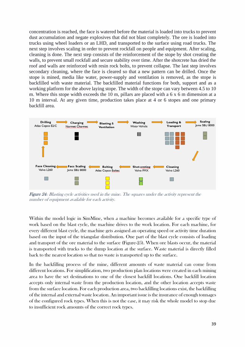
39

concentration is reached, the face is watered before the material is loaded into trucks to prevent

dust accumulation and negate explosives that did not blast completely. The ore is loaded into

trucks using wheel loaders or an LHD, and transported to the surface using road trucks. The

next step involves scaling in order to prevent rockfall on people and equipment. After scaling,

cleaning is done. The next step consists of the reinforcement of the stope by shot creating the

walls, to prevent small rockfall and secure stability over time. After the shotcrete has dried the

roof and walls are reinforced with resin rock bolts, to prevent collapse. The last step involves

secondary cleaning, where the face is cleared so that a new pattern can be drilled. Once the

stope is mined, media like water, power-supply and ventilation is removed, as the stope is

backfilled with waste material. The backfilled material functions for both, support and as a

working platform for the above laying stope. The width of the stope can vary between 4.5 to 10

m. Where this stope width exceeds the 10 m, pillars are placed with a 6 x 6 m dimension at a

10 m interval. At any given time, production takes place at 4 or 6 stopes and one primary

backfill area.

Within the model logic in SimMine, when a machine becomes available for a specific type of

work based on the blast cycle, the machine drives to the work location. For each machine, for

every different blast cycle, the machine gets assigned an operating speed or activity time duration

based on the input of the triangular distribution. One part of the blast cycle consists of loading

and transport of the ore material to the surface (Figure-25). When ore blasts occur, the material

is transported with trucks to the dump location at the surface. Waste material is directly filled

back to the nearest location so that no waste is transported up to the surface.

In the backfilling process of the mine, different amounts of waste material can come from

different locations. For simplification, two production plan locations were created in each mining

area to have the set destinations to one of the closest backfill locations. One backfill location

accepts only internal waste from the production location, and the other location accepts waste

from the surface location. For each production area, two backfilling locations exist, the backfilling

of the internal and external waste location. An important issue is the insurance of enough tonnages

of the configured rock types. When this is not the case, it may risk the whole model to stop due

to insufficient rock amounts of the correct rock types.

Figure 24:: Blasting cycle activities used in the mine. The squares under the activity represent the number of equipment available for each activity.

40

With the backfilling of waste material in the mine, specific loaders are used on the surface to

load the truck with waste. The same is true for the backfilling of the stopes where specific

loaders are used for only backfilling work. In the simulation model-specific machines only

work on the backfilling. The road trucks can do the ore transport and backfilling transport. In

the mine, the ore trucks are loaded on the surface with waste material for backfilling

underground stopes. In the SimMine simulation model, when a mine vehicle is assigned to

backfill work, the following will happen:

1. The vehicle will load itself and dumps at the backfill recipient location.

2. After the dump, the vehicle will get back to its original work.

3. During the temporarily backfill work, the vehicle will still have a reservation to the

original work location. This is so that no other vehicle will take its work, or if the

vehicle which takes the backfill work is a truck, then the loader which could work at

the original work location might become a loader without a truck if the truck wouldn’t

keep its reservation on its original work location, in which case the loader will start to

look for other work.

When the vehicle is a truck, a situation may arise depending on the configuration and

situation within the simulated mine as described below:

1. When the truck takes a temporarily backfill work which requires that a loader will

load onto the truck, a loader will also start to work at the temporarily assigned work

location.

2. When the backfill rock has been dumped to the backfill recipient, the truck will get

back to its original work location. This means that the loader working at the temporary

work location might be the only vehicle working there. This further means that it will

then search for other work.

3. If the loader at the temporary work location finds other work, the next time a truck

will search for temporarily backfill work, there might be no free loader, and thus, the

truck will not get a temporarily backfill work.

Figure 25: Simplified overview of how material is moved in the mine. Mainly ore transport is moved from the underground to

the surface and waste material from the surface to the underground.

41

Within the SimMine development package, one has the possibility to add operators into the

simulation model. The operator pool can be added under the operator tab in the software

package. Under the fleet properties within the advance, tab vehicle can be linked to the

operator pool. For this simulation study, each activity in the blast cycle is assigned one

operator for the task at hand; this assumption is not correct because some mining activities

such as shotcreting and charging need in general two operators. This assumption is going to

effect the result in a way that more operators are needed for the production then used in the

simulation. The assumption of using one operator and one machine for the activity is

incorrect. For the shotcreting activity, typically two machines and two operators are used. In

this simulation study, only one operator is used with one vehicle. This simplification of one

operator per activity is applied because otherwise, it can happen that an activity that uses two

operators cannot start working because it has to wait for two operators to come available in

the simulation. In the future the mine is planning on the person delivering the concrete to the

mine to continue directly to the shotcreting location. This would then make the assumption

correct of one person and one vehicle for the shotcreting activity. The operator function in

SimMine is new and not fully extensively tested.

Figure 26 :Operator pool selection within SimMine simulation software, where operators can be added into the simulation.

42

4.3 Model validation

Model verification, validation and testing are essential to understand the model accuracy. The

model verification, the process of ensuring that the model design has been transformed into a

computer model with sufficient accuracy, is more comfortable with simulation software. Model

verification was obtained by doing: self-inspection, and face validation.

Model verification is done using self-inspection, where one examines one's work (Banks, 1998).

This is also done with the help of another person because it is usually difficult to see your errors.

The face validation includes asking and checking the model with people knowledgeable about

the system under study, in order to judge whether the model and the results are reasonable.

In order to get information about the performance of the simulation and compare it to the real

mine, it is essential to use key performance indicators (KPI). These indicators are focused on the

organizational performance that is most critical for the success of the organization. KPIs are

nonfinancial measures that are measured frequently and are reported to management. These

indicators focus on specific activity (Parmenter, 2015). In this chapter, the focus will be on the:

total production of 2019, the monthly production, development meters and the number of blasts.

These indicators were chosen because they were available for the mining operation, and are

useful to compare the model to real-world operation.

The simulation period for the simulation study and model validation are similar. Next to visual

inspection, key statistics of the model are compared with the real data. The actual mine data is

defined by At, and the simulation result by St. Let’s start by defining the error as the actual

production data, minus the simulation result. It is important to notice that with this definition

when the actual production overshoots the demand, the error will be positive. In the same

manner, if the actual production undershoots the demand, the error will be negative and is

defined as:

𝑬𝒓𝒓𝒐𝒓 = 𝒆𝒕 = 𝑨𝒕 − 𝑺𝒕

(9)

The percentage error is a measurement of the discrepancy between the actual production and

the simulation result, and this error is then divided by the true value resulting in the relative error,

which is multiplied by 100 to get the percentage error:

𝑷𝒆𝒓𝒄𝒆𝒏𝒕𝒂𝒈𝒆𝒆𝒓𝒓𝒐𝒓 = |𝑨𝒕 − 𝑺𝒕𝑨𝒕

| × 𝟏𝟎𝟎

(10)

One can also define the average error as the bias:

𝑩𝒊𝒂𝒔 =𝟏

𝒏∑𝒆𝒕

(11)

Where n is the number of months for the actual production and the simulation results, the bias

refers to the tendency of a measurement process to over or underestimate the value of a

population parameter. As the errors can be positive and negative, they can offset each other. The

bias alone is not enough to evaluate the simulation precision, but a highly biased simulation result

can give the indication that something is wrong with the model.

43

The mean absolute deviation (MAD) of a dataset is basically the average distance between each

data point and the mean and provides information about the variability. In this comparison of

actual production data to simulation data, the MAD is calculated by taking the sum of the absolute

differences between the actual value and the simulation and divided this by the number of

observations.

𝑴𝑨𝑫 =∑ |𝑨𝒕 − 𝑺𝒕|𝒏𝒕=𝟏

𝒏

(12)

The mean Absolute Percentage Error (MAPE) is the average of absolute errors divided by the

actual observation values, and is expressed as the following:

𝑴𝑨𝑷𝑬 = ∑

|𝑨𝒕 − 𝑭𝒕|𝑨𝒕

𝒏𝒕=𝟏

𝒏× 𝟏𝟎𝟎

(13)

The formulas to calculate the different mean such as the: Bias, MAD, and MAPE, calculated

based on weeks or months of production, are not calculated over the entire range of the

simulation. Especially when calculating in weeks, n-2 is used for the beginning and the start of the

simulation. The summer production break in week-27 till week-30 are also not counted for the

mean errors. For the monthly based calculation n-1 is applied. This is because the amount of

resources is limited. Since deviations are expected during the simulation experiments, they will

likely occur at the beginning and the end of the simulation period. This bigger deviation is,

therefore excluded in the calculations.

The base-case using for trucks for transport, best representing the real mine in its current setup,

is used to validate the model. For validation, the key performance indicators used are wet tonnes

of ore, the development meters and the number of blasts. These KPIs were chosen because this

is the only data available to compare the simulation model to the real mine production. Input

parameters are based on the real mine system when available, such as most of the equipment

downtimes and activity times.

The simulation model is not an identical match to the actual mine, because there are so many

random activities that can occur during an underground cut and fill mining operations which

influence the production. For instance, the installation and maintenance of media such as, the

ventilation piping, electrical outlets and 5G network are not considered, while they take up time

from production. The media has to be installed before production to take place and continue.

These activities influence the production because the production at the location has to be stopped

for media installation. These activities are planned together with the production planning in order

to minimise the disturbance of the production. Proper ventilation and 5G network are essential

for the mining activity, to have fresh air from ventilation and communication connection from

the network, in case of an accident happening. Also ones every two to three weeks the production

can be stopped for multiple hours because of power loss due to a thunderstorms, flooding of the

access road during heavy rain in spring, or trucks slipping of the road during winter. The

underground ventilation and communication network are the determining factor for

underground mining operation to continue. The primary mining activities are considered in the

model.

44

4.3.1 Validation of yearly production

The first step in the validation is to check the total production difference over a one year

simulation period. The base-line simulation experiments are compared to the actual mine

production on a yearly basis. The real mine production in 2019 was 502,593 tonnes of wet ore.

The simulation model was run for 100 times. The Bias of these 100 simulation results was -272

tonnes with a MAD of 470 tonnes. The errors are calculated on the yearly production of each

simulation run. This means that the simulation produces 272 tonnes more per year than the

actual mine production, with a variability of 470 tonnes per year over the simulations.

The calculated errors can be obtained from Figure-27. The percentile errors are also calculated

for each simulation run and compared to the actual production in Figure-28. The absolute

percentage error (MAPE) over the number of replications is 0.094 percent. This means that the

total tonnage produced by the simulation model is close to reality.

45

0.000

0.050

0.100

0.150

0.200

0.250

0.300

0.350

1 4 7

10

13

16

19

22

25

28

31

34

37

40

43

46

49

52

55

58

61

64

67

70

73

76

79

82

85

88

91

94

97

10

0

PER

CEN

TILE

ER

RO

R

NUMBER OF REPLICATIONS

-2000.000

-1500.000

-1000.000

-500.000

0.000

500.000

1000.000

1500.000

1 4 7

10

13

16

19

22

25

28

31

34

37

40

43

46

49

52

55

58

61

64

67

70

73

76

79

82

85

88

91

94

97

10

0

CA

LCU

LATE

D E

RR

OR

NUMBER OF REPLICATIONS

Figure 27: The calculated error in production over one year simulation period for 100 simulation replications.

Figure 28 : The calculated percentile error over a one year simulation period for 100 replications.

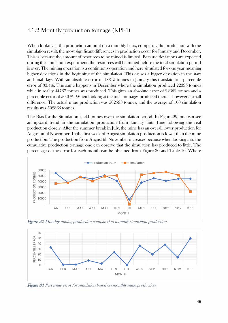
46

4.3.2 Monthly production tonnage (KPI-1)

When looking at the production amount on a monthly basis, comparing the production with the

simulation result, the most significant differences in production occur for January and December.

This is because the amount of resources to be mined is limited. Because deviations are expected

during the simulation experiment, the resources will be mined before the total simulation period

is over. The mining operation is a continuous operation and here simulated for one year meaning

higher deviations in the beginning of the simulation. This causes a bigger deviation in the start

and final days. With an absolute error of 18315 tonnes in January this translate to a percentile

error of 33.4%. The same happens in December where the simulation produced 22395 tonnes

while in reality 44757 tonnes was produced. This gives an absolute error of 22362 tonnes and a

percentile error of 50.0 %. When looking at the total tonnages produced there is however a small

difference. The actual mine production was 502593 tonnes, and the average of 100 simulation

results was 502865 tonnes.

The Bias for the Simulation is -44 tonnes over the simulation period. In Figure-29, one can see

an upward trend in the simulation production from January until June following the real

production closely. After the summer break in July, the mine has an overall lower production for

August until November. In the first week of August simulation production is lower than the mine

production. The production from August till November increases because when looking into the

cumulative production tonnage one can observe that the simulation has produced to little. The

percentage of the error for each month can be obtained from Figure-30 and Table-10. Where

0

10000

20000

30000

40000

50000

60000

J A N F E B M A R A P R M A J J U N J U L A U G S E P O K T N O V D E C

PR

OD

UC

TIO

N T

ON

NES

MONTH

Production 2019 Simulation

0

10

20

30

40

50

60

J A N F E B M A R A P R M A J J U N J U L A U G S E P O K T N O V D E C

PER

CEN

TILE

ER

RO

R

MONTH

Figure 29: Monthly mining production compared to monthly simulation production.

Figure 30: Percentile error for simulation based on monthly mine production.

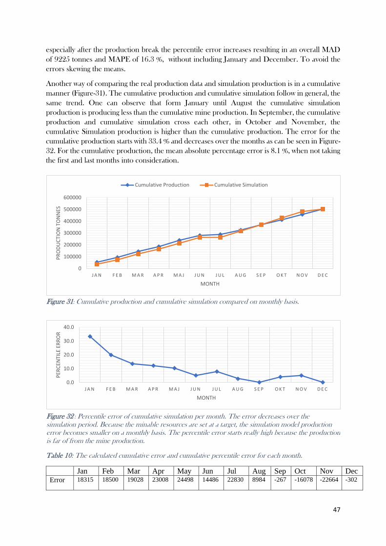
47

especially after the production break the percentile error increases resulting in an overall MAD

of 9225 tonnes and MAPE of 16.3 %, without including January and December. To avoid the

errors skewing the means.

Another way of comparing the real production data and simulation production is in a cumulative

manner (Figure-31). The cumulative production and cumulative simulation follow in general, the

same trend. One can observe that form January until August the cumulative simulation

production is producing less than the cumulative mine production. In September, the cumulative

production and cumulative simulation cross each other, in October and November, the

cumulative Simulation production is higher than the cumulative production. The error for the

cumulative production starts with 33.4 % and decreases over the months as can be seen in Figure-

32. For the cumulative production, the mean absolute percentage error is 8.1 %, when not taking

the first and last months into consideration.

Table 10: The calculated cumulative error and cumulative percentile error for each month.

Jan Feb Mar Apr May Jun Jul Aug Sep Oct Nov Dec Error 18315 18500 19028 23008 24498 14486 22830 8984 -267 -16078 -22664 -302

0

100000

200000

300000

400000

500000

600000

J A N F E B M A R A P R M A J J U N J U L A U G S E P O K T N O V D E C

PR

OD

UC

TIO

N T

ON

NES

MONTH

Cumulative Production Cumulative Simulation

0.0

10.0

20.0

30.0

40.0

J A N F E B M A R A P R M A J J U N J U L A U G S E P O K T N O V D E C

PER

CEN

TILE

ER

RO

R

MONTH

Figure 31: Cumulative production and cumulative simulation compared on monthly basis.

Figure 32 : Percentile error of cumulative simulation per month. The error decreases over the simulation period. Because the minable resources are set at a target, the simulation model production error becomes smaller on a monthly basis. The percentile error starts really high because the production is far of from the mine production.

48

Error

(%)

33.4 19.9 13.4 12.3 10.3 5.2 7.9 2.8 0.1 3.9 5.0 0.1

4.3.3 Development meters (KPI-2)

The second KPI used in this study is the development meters per month because this is recorded

in the mine. The Bias is 17 meters over one year, meaning that the actual production overshoots

the simulation model in development meters.

When comparing KPI-1 with KPI-2 a noticeable phenomenon is that simulation production is

higher in September and October than the production tonnage obtained from the previous

section in Figure-29, but the development meters are lower as can be obtained from Figure-33.

This can be caused by the input CAT files, where the face profile size might be different than in

reality. The CAT layout was created based on the plan and not on the reality because this was

not noted down with enough accuracy. Based on the changes as they occurred in 2019, the plan

was changed to fit the reality best.

The mean absolute deviation is 25.2 meter, and the mean absolute percentage error is 13.7 %,

without counting the month of July. They're supposed to be a production stop in July, however,

in reality, there was a development of 40 meters compared to the 0 meters in the model resulting

in a percentile error of 100% for this month (Figure-34 and Table-12). This is because the original

plan had no development meters or production planned in July, therefore the simulation has no

production. In reality there was some production activity in July resulting in this large error.

0

100

200

300

400

500

J A N F E B M R T A P R M E I J U N J U L A U G S E P O K T N O V D E C

DEV

ELO

PM

ENT

(M)

MONTH

Mine Development Simulation Development

0

50

100

150

J A N F E B M R T A P R M E I J U N J U L A U G S E P O K T N O V D E C

PER

CEN

TILE

ER

RO

R

MONTH

Figure 34 : Percentile error for development meters per month.

Figure 33: Development meters per month for the mine and simulation model.

49

Table 11: Error and percentile error calculated for development meters.

Jan Feb Mar Apr May Jun Jul Aug Sep Oct Nov Dec Error 34 43 56 -12 -16 -13 40 3 72 10 -20 2

Error

(%)

8.4 11.8 12.3 3.2 4.6 4.4 100 1.1 21.4 2.7 5.7 0.6

4.3.4 Number of blasts (KPI-3)

Another KPI used is the number of blasts to compare the mine with the simulation model. This

KPI was measured in weeks because the blasts are planned per week, and therefore it was more

convenient to reach on a weekly basis. The biggest deviations are in the beginning and end of the

simulation and during the break period in the summer (Figure-35). The bias of the simulation is

0.7 blasts, when not taking the beginning, break and end period into consideration. The average

blasts per week in the real mine is 18 blasts per week and the simulation period has 17 blasts per

week. This difference is possible because in the real mine the blasts are sometimes fine-tuned at

boundaries of ore and waste or pillar boundaries resulting in more blasts, this precision is not

considered in the simulation model.

The percentile error for the beginning and the end of the simulation period are large (Figure-

36). In the first week, the error is 31.6 %, in week 27 is another peak of 66.7% error, also in week

51 and 52, the errors are large with respectively 55.5 % and 93.8 %. These errors are large because

the simulation starts and ends over 2019, but in reality, the mining process is a continuous

process. Therefore, when not considering these two weeks at the start and end of the simulation,

the MAPE becomes 13.1 %. The Bias is 0.74 and the MAD 2.26.

0

50

100

1 3 5 7 9 1 1 1 3 1 5 1 7 1 9 2 1 2 3 2 5 2 7 2 9 3 1 3 3 3 5 3 7 3 9 4 1 4 3 4 5 4 7 4 9 5 1PER

CEN

TILE

ER

RO

R

WEEK NUMBER

0

5

10

15

20

25

30

1 3 5 7 9 1 1 1 3 1 5 1 7 1 9 2 1 2 3 2 5 2 7 2 9 3 1 3 3 3 5 3 7 3 9 4 1 4 3 4 5 4 7 4 9 5 1

NU

MB

ER O

F B

LAST

S

WEEK NUMBER

Mine Blast Simulation Blasts

Figure 36: Percentile error per week for the number of blasts per week.

Figure 35: Number of blasts for the mine production and simulation on weekly basis.

50

4.4 Assumptions and simplifications of the model

For this simulation model, several assumptions and simplifications were made, while some

have been mentioned in previous chapters, they will be all mentioned in this chapter.

Simplifications:

• The model includes machine breakdowns and maintenance, but in a way still

represents an ideal state of the mine. Media activities, such as the installation of the

ventilation tubes, are, for instance, not considered in the simulation, while they

influence the production.

• In the first instance, the backfilling process was not included in the process and later

added. Because there was no documentation available on how much waste tonnes was

deposited per location, the waste backfill is based on the original plan. In 2018 the

waste filling was behind schedule, part of this waste was backfilled in 2019. No exact

record was found and therefore not considered in the model.

• The blasting cycle process can start as soon as a machine for the process becomes

available. If there are, for instance, two blasts planned at S517 and drilling work is

done for both locations. In reality, this might not be possible, because the number of

machines is limited by the available power slots at the power station. In most areas,

the mine has one power station per stope.

• For the shift working schedules, preparation, break and leaving time are subtracted

from the start and end time of the shift. This results in a shorter shift duration as used

for the simulation. It was not studied what the duration was of preparation and leaving

time for the operators. Based on experience, this time was assumed 45 minutes per

day.

• The measured tramming speeds were assumed to be all the same for the mining

equipment. There is some driving speed difference in a drilling machine or a bolting

machine because the long boom of the drilling machine makes it slower in

manoeuvring in corners of the road. For this simulation, the travel speed was all set to

17 km/h. The truck speeds were measured over different locations and distanced in the

mine. The average truck speed going loaded uphill was 17km/h, downhill with 24km/h

and on the flat straight roads 30 km/h.

Assumptions:

• The mine is limited by the number of operators for the machines and not by the

number of machines. The original production is with the usage of four trucks while

seven are available. In the simulation model, all the machines are used.

• General ventilation time was assumed. In reality, ventilation time is based on the

number of blasts. The blasts are done after the evening shift has finished, and therefore

does not affect the simulation in any way.

51

5 Results

During the simulation study, one finding was that the mine currently has problems with the

transport, due to the fact that transportation is limited by the number of trucks used. Because of

this discovery, multiple simulations scenarios were studied based on the different number of

trucks. The first scenario simulates the mine in its current state using four trucks for ore and waste

transport. There were twenty scenarios created using; 4,5,6,7 and 8 trucks and 10 to 15 operators

for the simulation study. The number of trucks for financial analysis was limited to seven trucks

because they are available at the mine location.

The first part of the results, consist of the activity times as measured in the mine, and simulation-

based results that were analysed using the PIP bottleneck identification method to determine the

bottleneck in the production. In section 5.1, the scenarios are compared to the average waiting

time, workload, and duration. In section 5.2 and 5.3, results are concerning the cycle time, and

the production presented graphically and in tables. The last part of the results, section 5.4,

focusses on the financial aspect of the simulated production for the different number of operators

and trucks.

5.1 Production Bottleneck Identification

The bottleneck or constraint in the mining process is being analysed using the PIP method, as

mention in Chapter-2.1.2. This method involves looking at the following equipment activities:

• Average waiting time, where the machine with the longest average waiting time is the

constraint.

• Average workload looking at the idle ratio, where the machine with the highest workload

and the shortest idle time is considered to be the constraint of the system.

• Active duration, the machine with the longest processing time is viewed as the bottleneck.

When activity data is consistently measured over a historical period, this data can be used to

determine the average waiting time, workload and active duration. Because this is not the case for

the mining operation a simulation study was created to find and research the bottleneck with

multiple scenarios. To identify the bottleneck for the current mining situation, data such as the

machine activity times such as the Gantt-Scheduler data can be used. Because some of the input

data were not consistently recorded throughout the year, this could give a wrong indication.

However, based on the available measured data, one can show the active duration per machine

type without using the simulation results. This is done in section 5.11 and 5.1.2, before analysing

the simulation results in later sections, since this can already give an indication on the bottleneck.

5.1.1 Gantt scheduler bottleneck identification (active duration method)

When looking at the Gantt Scheduler data measured over 2019 presented in Figure-37, one can

observe that the truck transport has a total activity of 5057 hours, and is the largest total

measured time. This would indicate, based on Roser et al. (2003), that the machine with the

52

longest processing time is the constraint of the system. This would suggest that the trucks

transport is the bottleneck within the production. This would also indicate that the second

bottleneck would be the bolting activity. It is important to keep in mind that this data was not

consistently measured over the year. The loading activity is much shorter than truck transport.

In the case of this mine, the loading activity is linked at the truck transport.

Figure 37: Gantt-Scheduler activity times of the blast cycle measured over 2019, data measurements were not consistently measured over the period of a year. The truck transport shows the biggest active duration, and can be therefore indicated as a bottleneck.

5.1.2 Maximo data bottleneck identification (active duration method)

Total electrical and diesel engine hours were extracted from Maximo maintenance software. The

software measures the electrical and engine hours separately for each machine. The engine

hours, especially the electrical hours for the mining machines, can give an indication for the active

duration because in general the machine only works at a location on electricity. For loading and

truck hauling, the diesel hours are representable of the active duration. Based on the measured

results of Maximo, the longest electrical engine hours are from the scaling equipment with 6203

hours, and secondly the bolting activity with 5786 hours (Figure 38). The engine hours for the

washing activity are large with 5409 for 2019 because this is not only used for the blast cycle but

general dust maintenance in the mining operation. Because of this, the machine is used

throughout the whole mine resulting in high activity hours. The diesel hours of 2019 show that

the loading and truck transport has the largest amount of hours (Figure 39), indicating the

bottleneck with respectively 11,082 hours for loading and 10,854 hours for transportation. When

looking at the total engine hours, it becomes clear that for the mining operation the potential

production bottleneck involves the loading and hauling operations presented in Figure-40.

0 1000 2000 3000 4000 5000 6000

Cleaning

Washing

Shotcreting

Charging

Scaling

Drilling

Loading

Bolting

Truck transport

TIME (HOURS)

AC

TIV

ITY

0 1000 2000 3000 4000 5000 6000 7000

Shotcreting

Charging

Drilling

Bolting

Scaling

DURATION (HOURS)

AC

TIV

ITY

Figure 38: Total electrical engine hours measured over 2019 based on the Maximo software.

53

0 2000 4000 6000 8000 10000 12000

ChargingDrillingScalingBolting

ShotcretingWashing

TransportLoading

DURATION (HOURS)

AC

TIV

ITY

0 2000 4000 6000 8000 10000 12000

Charging

Scaling

Shotcreting

Bolting

Drilling

Washing

Transport

Loading

DURATION (HOURS)

AC

TIV

ITY

Figure 40 : Total diesel engine hours measured over 2019 based on the Maximo software.

Figure 39 : Total engine hours, consisting out of the electrical hours and diesel hours.

54

5.1.3 Simulation based waiting time method

The simulation results performed using SimMine allows the identification of the production

bottleneck. In order to improve the mining system, the bottleneck has to be investigated. As

mentioned in Chapter-4.1, the bottlenecks are identified by the longest average waiting time, the

largest average workload, and longest active duration.

The first type of bottleneck identification derived from the simulation study is the longest average

waiting time. The waiting times are a process introduced because of the additional waiting to be

processed at each step, which results in delays. The theory of constraints suggests that all

improvements efforts should be focused on the bottleneck because an hour lost in the bottleneck

is an hour lost in the entire end to end process. For this simulation study, the activity wait time is

the amount a specific activity has to wait until it starts working. This waiting time will be counted,

even if no vehicle is scheduled to run. For example, when there are two faces, each with loading

and transport activity, and someone working at the face, when the lunch break of one-hour starts,

all vehicles will stop for lunch. This means that each of the faces will have one hour of waiting

time because no work was done during the break. After the lunch break is over, the total waiting

time for the loading and transport activity is translated to two hours, one hour of waiting time for

each face.

Figure-41 presents the total waiting time for each activity for the simulated year of 2019. The

longest waiting time is introduced with loading and transport activity. This would then indicate

the first bottleneck in the production is the loading and hauling activity. This would also suggest

that the machines responsible for the activity, the trucks, have not enough capacity and therefore

impact the other machines cycles. As can be seen in Figure-41, it took overall 13,991 hours of

waiting time for the trucks and loaders. This indicates that the loading and transport processes

had to wait the longest time for the loaders and trucks to start and complete their work.

Figure 41 : Average waiting time based on the simulation model with the mine setup of 2019. The loading and transport show the longest waiting time indicating the production bottleneck.

0 2000 4000 6000 8000 10000 12000 14000 16000

Shotcreting

Face cleaning

Cleaning

Charging

Face scaling

Scaling

Drilling

Bolting

Washing

Loading and transport

DURATION (HOURS)

AC

TIV

ITY

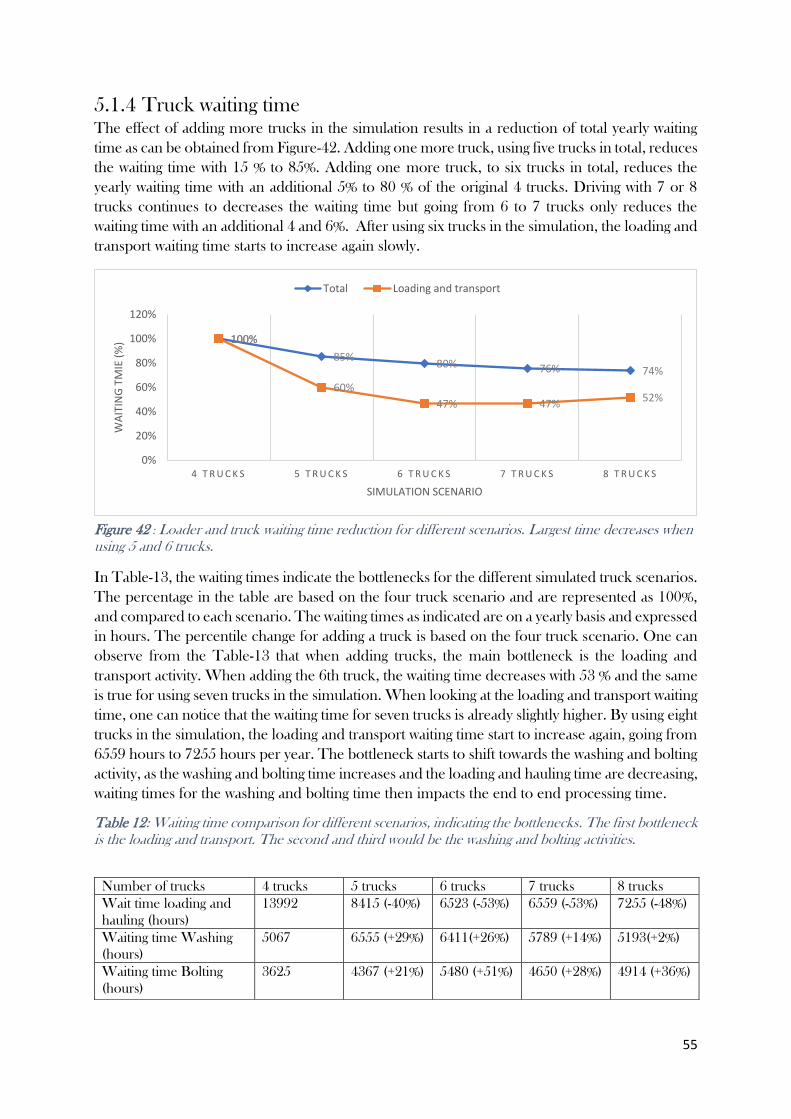
55

5.1.4 Truck waiting time The effect of adding more trucks in the simulation results in a reduction of total yearly waiting

time as can be obtained from Figure-42. Adding one more truck, using five trucks in total, reduces

the waiting time with 15 % to 85%. Adding one more truck, to six trucks in total, reduces the

yearly waiting time with an additional 5% to 80 % of the original 4 trucks. Driving with 7 or 8

trucks continues to decreases the waiting time but going from 6 to 7 trucks only reduces the

waiting time with an additional 4 and 6%. After using six trucks in the simulation, the loading and

transport waiting time starts to increase again slowly.

In Table-13, the waiting times indicate the bottlenecks for the different simulated truck scenarios.

The percentage in the table are based on the four truck scenario and are represented as 100%,

and compared to each scenario. The waiting times as indicated are on a yearly basis and expressed

in hours. The percentile change for adding a truck is based on the four truck scenario. One can

observe from the Table-13 that when adding trucks, the main bottleneck is the loading and

transport activity. When adding the 6th truck, the waiting time decreases with 53 % and the same

is true for using seven trucks in the simulation. When looking at the loading and transport waiting

time, one can notice that the waiting time for seven trucks is already slightly higher. By using eight

trucks in the simulation, the loading and transport waiting time start to increase again, going from

6559 hours to 7255 hours per year. The bottleneck starts to shift towards the washing and bolting

activity, as the washing and bolting time increases and the loading and hauling time are decreasing,

waiting times for the washing and bolting time then impacts the end to end processing time.

Table 12: Waiting time comparison for different scenarios, indicating the bottlenecks. The first bottleneck is the loading and transport. The second and third would be the washing and bolting activities.

Number of trucks 4 trucks 5 trucks 6 trucks 7 trucks 8 trucks

Wait time loading and

hauling (hours)

13992 8415 (-40%) 6523 (-53%) 6559 (-53%) 7255 (-48%)

Waiting time Washing

(hours)

5067 6555 (+29%) 6411(+26%) 5789 (+14%) 5193(+2%)

Waiting time Bolting

(hours)

3625 4367 (+21%) 5480 (+51%) 4650 (+28%) 4914 (+36%)

100%

85%80% 76% 74%

100%

60%

47% 47%52%

0%

20%

40%

60%

80%

100%

120%

4 T R U C K S 5 T R U C K S 6 T R U C K S 7 T R U C K S 8 T R U C K S

WA

ITIN

G T

MIE

(%

)

SIMULATION SCENARIO

Total Loading and transport

Figure 42 : Loader and truck waiting time reduction for different scenarios. Largest time decreases when using 5 and 6 trucks.

56

5.1.5 Simulation based workload method

Figure-43 illustrates the fleet utilization per vehicle type in percentage; this can also be referred to

as the average workload and is the second step in the bottleneck identification. This KPI

compares to the previous KPI, that they both include the waiting time. The idling time of the

machine is defined as the work that a machine is scheduled to work but can’t find work. For the

workload it is important to look at the ratio between working time and idle time.

The base case scenario using four trucks mimics the current mine equipment setup of available

machines in the production. In Figure-43, going from left to right, one can observe that the work

percentage increase, and the idle percentage decreases. The four truck have the highest work

percentage and lowest idle percentage with 21 %. The idle time can be described as the time

when the vehicle is scheduled to work but hasn’t found any work. The idle time for the other

equipment is really high because all the equipment was used in the simulation study. In the mining

operation, next to the production activities, equipment is also used for general maintenance in

the mine. Think for example about, roof and wall support improvements of the haul roads that

have to be carried out, ventilation shafts or small areas that are created near production areas that

are used for rescue chambers, vehicle passing points, water pumps and reservoirs etc.

Because the trucks show the lowest idle time, this would mean that the trucks are the bottleneck

in the production. Hauling and loading require the correct number of trucks and loaders.

Because the idle time of the trucks with 21% is considerably smaller than 65.9% of the loaders,

this results in the truck capacity being the limiting factor within the production. One can observe

from Figure-44, the work and idle ratio for different numbers of trucks used in the simulation.

70.70%60.00%

49.80% 42.80% 37.80% 33.70%

7.60% 21.00% 32.30% 40.40% 45.70% 50.30%

11.20% 11.20% 11.20% 11.20% 11.20% 11.20%10.50% 7.80% 6.60% 5.70% 5.30% 4.70%

0.00%

20.00%

40.00%

60.00%

80.00%

100.00%

120.00%

3 trucks 4 trucks 5 trucks 6 trucks 7 trucks 8 trucks

Work Idle Break Downtime

2.3% 2.4% 9.4% 15.4% 17.6% 20.0% 21.3%

60.0%86.2% 84.7% 79.3% 64.9% 67.7% 55.7%

65.9%

21.0%

11.2% 11.2% 11.2%11.2% 11.2%

11.2%11.2% 11.2%

0.3% 1.7% 0.0% 8.5% 3.4% 13.0% 1.5% 7.8%

0.0%

20.0%

40.0%

60.0%

80.0%

100.0%

120.0%

Watervehicle

Mulltifunctional

vehicle

Charger Face drill rig Scaler Bolter Loader Truck

Work Idle Scheduled break Downtime

Figure 43 : Truck utilization for different numbers of trucks used in the simulation.

Figure 44 : Fleet utilization per vehicle type in percentage.

57

5.1.6 Simulation active duration method

The third step in the bottleneck identification method is investigating the active duration or also

referred to as active processing time. The basic idea of this method is that a long process, active

without interruptions, is more likely to be the bottleneck in the system. The average active

duration method measures the average active time a process is active. In the case of the mining

operation, it is the loading and transport activity, showing a much longer active period than any

other process. This average active period is the sum of all cycle times without interruption by

introduced waiting times. Figure-45, shows the active duration of the mining system with ten

processes. The lowest activity time is found for the washing of 137 hours and the highest activity

time of 8048 hours for loading and transport. This means that loading and transport has the

longest active cycle time.

When adding extra trucks into the simulation the active time for the loading and hauling time

decreases. With five trucks the active time decreases with 16% and with six trucks 30 % to the

original four trucks that are being used. When using eight trucks the activity time of the loading

and transport activity is decreased with 46 %. The activity showing the second highest activity

times is the rock bolting activity, and thirdly the drilling activity. When adding trucks into the

simulation there are no major changes in the times of the rock bolting and drilling activities. Based

on the active duration method, the loading and hauling activity continuous to stay to have the

longest active duration in the production. When checking the active loading and hauling time of

4381 hours, using 8 trucks, and comparing them to the 3627 hours for the bolting activity, one

can observe that the bottleneck is shifting toward the bolting activity.

0 1000 2000 3000 4000 5000 6000 7000 8000 9000

Washing

Face cleaning

Face scaling

Cleaning

Shotcreting

Charging

Scaling

Drilling

Bolting

Loading and transport

DURATION (HOURS)

AC

TIV

ITY

Figure 45 : Active duration for each activity using 4 trucks.

58

5.1.7 Bottleneck comparison

The current bottlenecks in the production were researched using different methods, based on

measured input data from the Gantt Scheduler and the Maximo data. For the simulation result,

Gantt data was recreated with the simulation model and analysed for the different scenarios. In

the results, bottleneck-1 is presented as the primary bottleneck. The second and third bottleneck

can become potentially the first bottleneck when the loading and transport activity is improved.

For each method, the loading and hauling activity was discovered to be the first bottleneck.

Second and third bottlenecks were changing depending on the method. For the mining situation

using four trucks, the bottlenecks were found to be as presented in Table-15.

For each method, the loading and hauling activity was found to be the production bottleneck.

The Gantt and Maximo data was analysed data from the mine. The waiting time, workload and

active duration were based on the simulation results. Because the Gantt scheduler data was not

consistently measured, this result is less reliable.

Table 13: Bottleneck identification summary of the mining situation using 4 trucks.

Method Gantt data

active

duration

Maximo data

Active

duration

Simulation

waiting time

Simulation

workload

Simulation

active

duration

Bottleneck 1 Loading &

transport

Loading &

transport

Loading &

transport

Loading &

transport

Loading &

transport

Bottleneck 2 Bolting Washing Washing Bolting Bolting

Bottleneck 3 Drilling Drilling Bolting Scaler Drilling

When analysing the Gantt data, Maximo data, waiting time, workload, and active duration the

first bottleneck stays consistent the loading and hauling activity.

All yearly active duration times decrease when adding trucks into the simulation, as can be

obtained from Figure-46. This shows the active duration for each additional truck, in a visual

0 1000 2000 3000 4000 5000 6000 7000 8000 9000

Washing

Face cleaning

Face scaling

Cleaning

Shotcreting

Charging

Scaling

Drilling

Bolting

Loading and transport

Active duration (hours)

Act

ivit

y

8 trucks 7 trucks 6 trucks 5 trucks 4 trucks

Figure 46 : Active duration for each activity using different truck numbers over one year simulation period.

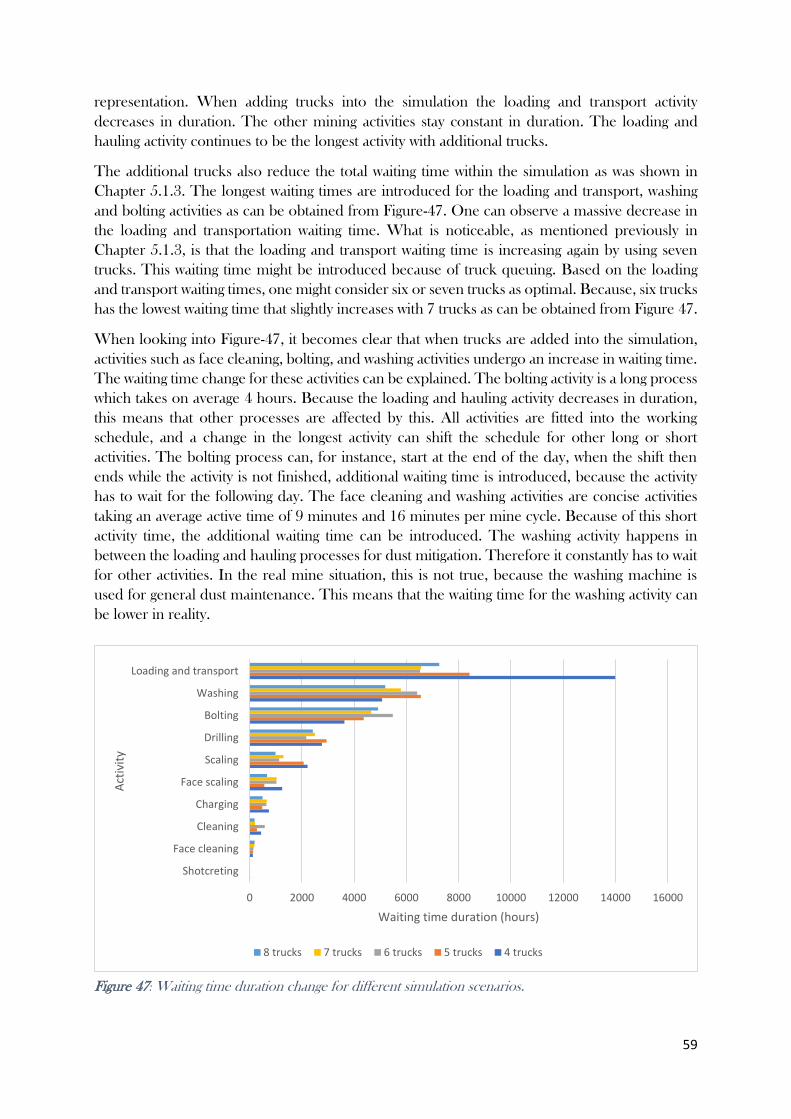
59

representation. When adding trucks into the simulation the loading and transport activity

decreases in duration. The other mining activities stay constant in duration. The loading and

hauling activity continues to be the longest activity with additional trucks.

The additional trucks also reduce the total waiting time within the simulation as was shown in

Chapter 5.1.3. The longest waiting times are introduced for the loading and transport, washing

and bolting activities as can be obtained from Figure-47. One can observe a massive decrease in

the loading and transportation waiting time. What is noticeable, as mentioned previously in

Chapter 5.1.3, is that the loading and transport waiting time is increasing again by using seven

trucks. This waiting time might be introduced because of truck queuing. Based on the loading

and transport waiting times, one might consider six or seven trucks as optimal. Because, six trucks

has the lowest waiting time that slightly increases with 7 trucks as can be obtained from Figure 47.

When looking into Figure-47, it becomes clear that when trucks are added into the simulation,

activities such as face cleaning, bolting, and washing activities undergo an increase in waiting time.

The waiting time change for these activities can be explained. The bolting activity is a long process

which takes on average 4 hours. Because the loading and hauling activity decreases in duration,

this means that other processes are affected by this. All activities are fitted into the working

schedule, and a change in the longest activity can shift the schedule for other long or short

activities. The bolting process can, for instance, start at the end of the day, when the shift then

ends while the activity is not finished, additional waiting time is introduced, because the activity

has to wait for the following day. The face cleaning and washing activities are concise activities

taking an average active time of 9 minutes and 16 minutes per mine cycle. Because of this short

activity time, the additional waiting time can be introduced. The washing activity happens in

between the loading and hauling processes for dust mitigation. Therefore it constantly has to wait

for other activities. In the real mine situation, this is not true, because the washing machine is

used for general dust maintenance. This means that the waiting time for the washing activity can

be lower in reality.

0 2000 4000 6000 8000 10000 12000 14000 16000

Shotcreting

Face cleaning

Cleaning

Charging

Face scaling

Scaling

Drilling

Bolting

Washing

Loading and transport

Waiting time duration (hours)

Act

ivit

y

8 trucks 7 trucks 6 trucks 5 trucks 4 trucks

Figure 47: Waiting time duration change for different simulation scenarios.

60

5.2 Cycle time

The change in cycle time is another result of the difference in the number of trucks used for the

simulation. The average cycle time of the base case is compared to the average cycle time of each

scenario. The change in the average cycle time is shown in Figure-48. By adding an additional

truck, the cycle time continues to decrease. For the case of five trucks, the cycle time decreases

by -7.1 % and the waiting time by -14.6 %. For the case of six trucks, the total cycle time decreases

by -13% and -20.2% in waiting time. By adding a 7th or 8th truck, one can observe that the curves

start to flatten out. This result indicates that an increase in production is possible, because a

decrease in the blast cycle time translate to a production increase. Since it takes less time to mine

a similar amount of material.

The mine cycle time stays constant for each mining activity, except for the loading and hauling

operation. In Appendix-A, the average waiting times are presented in a table for each activity in

the blasting cycle.

5.3 Mine production

The possible increase in production is probably the most exciting effect on the added trucks in

production. Production increase will lead to a financial benefit that can offset the operational

costs of additional trucks and miners. The production increase for this research is based on the

simulation model. The ore production was limited by the production plan; this would result in a

production target that was reached in week 49 of 2019. Because of this, in the simulation model,

the average weekly production was added to produce towards week 52. An important note is that

the mine production is based on the long term and short term plans. The amount of material that

can be produced is based on the permits that allow a certain production tonnage. In reality

without changing the production plans and permits, one cannot merely produce more ore.

100%

85%80% 76% 74%

100%

60%

47% 47%52%

100%93%

87% 85% 81%

0%

20%

40%

60%

80%

100%

120%

4 T R U C K S 5 T R U C K S 6 T R U C K S 7 T R U C K S 8 T R U C K S

CYC

LE T

MIE

CH

AN

GE

(%)

SIMULATION SCENARIO

Total waiting time Loading and transport waiting time Total cycle time

Figure 48 : Cycle time change for the total cycle time, waiting time and loading and transport wating time within the cycle.

61

The production in an underground mine depends on a complex system; a production gain in

one specific process will not automatically lead to an overall production increase. The bottleneck

in the mining process, will constrain and dictate the mine production (Mathu, 2014). According

to a Boliden hypothesis, this was the Bolting operation, but in this research, it was found that the

production is constraint by the transport capacity. This capacity can be increased by increasing

the transport. In order to investigate the size of the gap between the next bottleneck, the PIP

bottleneck detection method was used, as mentioned in the previous section.

The yearly weekly production for each scenario using the maximum production capacity was

analysed for each scenario and compared to the case, consisting out of 4 trucks. The constructed

and analysed simulation scenarios were constructed based on the planned resources of the mine,

but for measuring the potential production increase, additional ore was added. The following

scenarios were simulated, where for each scenario, the number of trucks was kept the same and

operators were added:

• Four trucks and 9 to 15 operators.

• Five trucks and 10 to 15 operators.

• Six trucks and 10 to 15 operators.

• Seven trucks and 10 to 15 operators.

The usage of eight trucks was also simulated, but directly showed no change in production. Also,

the waiting time analyses showed that with more than seven trucks the waiting time for the number

of trucks start to increase. In Figure-49, one can observe the potential increase in production

based on the number of trucks and operators. The positive trend of production increase stops

after using seven trucks. (was marked but no comment written)

In Figure-50, one can observe in general that the number of trucks shows the largest increase in

production. For the current mine situation using four trucks, the number of operators, employing

more than ten operators, don’t deliver to much change in production. Using five trucks and 13

operators, the production increases with +9.41%. Using more operators, don’t show a drastic

increase in production. Using six trucks and 13 operators can increase production with +15.09%.

When using seven trucks and 14 operators, the production can increase towards +19.35%. A

summary of the production and weekly production can be found in Table-16. The selected

scenarios were chosen based on the revenue mentioned in section 5.4.3.

87%100%

109% 115% 119% 119%

0%

20%

40%

60%

80%

100%

120%

140%

Simulation 3trucks

4 trucks and 10operators

5 trucks and 13operators

6 trucks and 13operators

7 trucks and 14operators

Simulation 8trucks

Pro

du

ctio

n (

%)

Figure 49 : Potential production change when simulating for different scenarios.

62

Table 14: Production tonnage for selected scenarios.

Scenario 4-trucks and 10-

operators

5-trucks and 13-

operators

6-trucks and 13-

operators

7 trucks and 14-

operators

Total

Production

(tonnage)

509746 t 550336 t

(+9.41%)

578928 t

(+15.09%)

600325 t

(+19.35%)

Weekly production

Minimum 5521 t 5698 t 6401 t 5198 t

Q1 9370 t 9997 t 10741 t 10797 t

Q2 11234 t 11545 t 12488 t 13536 t

Q3 12277 t 13172 t 13715 t 14116 t

Max 13948 t 15144 t 16338 t 17440 t

Mean 10620 t 11465 t 12061 t 12507 t

Standard

deviation

2091 t 2280 t 2474 t 2698 t

-0.55 0.00 0.01 0.01 0.01 0.01 0.01

7.158.26 8.42

9.41 9.42 9.43

12.9213.61 14.22

15.09 15.12 15.1216.46 16.50

18.63 18.75 19.35 19.38

-5.00

0.00

5.00

10.00

15.00

20.00

25.00

9 1 0 1 1 1 2 1 3 1 4 1 5

PR

OD

UC

TIO

N C

HA

NG

E (%

)

NUMBER OF OPERATORS

4 trucks

5 trucks

6 trucks

7 trucks

Figure 50 : Production change in percentages for different numbers of operators and trucks.

63

5.4 Financial analysis

In this chapter, the financial cost and possible production increase are evaluated to get an

estimation of the costs for each scenario. A common method to evaluate mining projects is by

using the discounted cashflow model. With this method the NPV and IRR can be calculated. For

this thesis, it was decided to calculate the net present value, without including new CAPEX

because the CAPEX for the mine is small and the additional trucks, 7 in total, are already

available. The second reason being that the mine was simulated over 2019 and these costs were

used to create the financial model. The financial model is created to calculate the cost for each

scenario in order to determine the lowest cost per tonne of ore.

For the revenue evaluation, a Net Smelter Return (NSR) is calculated. The NSR is basically the

value in Swedish Kronor (SEK) for each gram of each contained product or by-product. Because

the material is a combined product, the product value is described as tonnages in terms of SEK/t.

In Table-17, the NSR factors are provided for each element over the Life of Mine (LOM).

Table 15: Revenue evaluation.

Element NSR (SEK/t) Average LOM

grade (g/t)

Average LOM

NSR (SEK/t)

LOM revenue

contribution

Au 247 3.29 813 96%

Ag 1.4 10 14 1.7%

Te 0.13 172 22 2.6%

5.4.1 Cost and revenue factors The marginal cut-off grade for a resource to be defined is 300 SEK/t. The breakeven mining cut-

off grade is 525 SEK/t; this is also used for the Mineral resources and reserves estimation. When

mining takes place under this cut-off, it is because lower grade ore is mined to gain access to the

high-grade ore.

The cost of additional trucks mainly consists of maintenance, labour, depreciation and fuel costs.

The financial model only considered direct costs and no overhead costs. Some of the basic input

costs can be found in Table-18. The transportation costs and total cycle cost exclude the operator

costs as mentioned in the table, operational costs are calculated separately. The total cycle cost

includes the blast cycle, media, drift ventilation and other relevant costs.

Table 16: Basic input costs.

Transportation costs

Loading underground 9.51 SEK/t Staff costs

Loading wate rock 4.51 SEK/t mine worker 900,000.00 Kr/year

backfill loader 6.54 SEK/t Blast cycle costs

1 Truck 2,364,725.00

SEK Total cycle costs (no loading and

hauling)

43.6 Kr/ton

64

5.4.2 Sensitivity analysis

Sensitivity analysis is used as a tool in financial modelling to analyse how the different values of a

set of variables affect the depended variable under specific conditions. This analysis is also known

as a what-if simulation exercise and is used to predict outcomes of a particular action when it is

performed under certain conditions. This process of testing sensitivity for input while keeping the

rest of the inputs constant is repeated until the sensitivity for each of the important inputs is

obtained. This means that the higher the sensitivity figure, the more sensitive the output is to

change of input. For the financial part of this study, the conditions under which the revenue

change for the number of trucks and the number of operators have been analysed. The analysis

in Figure-51 shows that the ore price and ore production have the most considerable influence

on the revenue. The number of operators and the number of trucks has the smallest impact on

revenue. However, one can observe that the number of operators shows more sensitivity towards

the revenue change. The blast cycle OPEX include the blast cycle activities with ventilation and

media costs.

0

100000000

200000000

300000000

400000000

500000000

600000000

700000000

800000000

900000000

1E+09

50% 70% 90% 110% 130% 150%

Rev

enu

e (S

EK)

Change of input

Ore production

Number of operators

Blast cycle OPEX

Truck OPEX

Ore price

Figure 51 : Sensitivity analysis of Revenue for different inputs.

65

5.4.3 Cost and revenue analysis

When analysing the revenue for each scenario, the revenue changes between the number of

operators are small. The ore production has an enormous sensitivity and is linked to the number

of trucks because the amount of trucks is the bottleneck determining ore production. For each

scenario, the maximum total ore production was simulated and used for the financial analysis.

The result of the revenue change for the truck number and operator size per shift can be found

in Figure-52. Each percentage is based on the scenario of four trucks and ten operators. When

selecting the highest revenue for the truck number the following operator sizes can be found: four

trucks & ten operators, five trucks & thirteen operators, six trucks & 13 operators, seven trucks

and 14 operators.

100.0% 99.7% 99.3% 98.9% 98.6% 98.2%

108.9%110.2% 110.1%

111.2% 110.9% 110.5%

117.1% 117.8% 118.4% 119.3% 119.0% 118.6%

122.0% 121.7%

124.5% 124.4% 124.9% 124.6%

95.0%

100.0%

105.0%

110.0%

115.0%

120.0%

125.0%

130.0%

10 11 12 13 14 15

Re

ven

ue

ch

ange

Number of operators

4 trucks

5 trucks

6 trucks

7 trucks

Figure 52 : Twenty four scenarios were simulated and the revenue change for each scenario presented. On the y-axis the revenue change is presented in percentage and on the x-axis the number of operators. The lines represent the truck numbers. With 7 trucks and 14 operators the highest revenue of 124.9% is found.

66

From Figure-53, one can observe that the different costs per tonne for each simulated scenario

as presented. When using four trucks, one can observe that the cost per tonne increases in a

straight line from 518 SEK towards 536 SEK. When watching the cost per tonne using five or six

trucks, the lowest price can be found using 13 operators. When changing towards seven trucks,

the lowest cost per tonne is found when using twelve operators. However, when looking at the

revenue for seven trucks in the previous section, the highest value can be found with 14 operators.

The extra cost of having two additional people in the shift outweighs the extra tonnage when

calculating the cost per tonne but still results in higher revenue.

Based on the previously mentioned revenues and mining costs, the ideal scenarios were selected.

All the scenario were analysed, and the highest revenue values were found when using: seven

trucks and 14 operators. The lowest cost per tonne was found using seven trucks and twelve

operators. In figure-54, one can observe the positive change in revenue in percentage. In Figure-

55, one can see the decrease in mining cost per tonne for the optimal scenario based on the truck

number. Where one can observe that the cost per ton change is minimal when using seven truck

and 12,13 or 14 operators change from -12% toward -11.4 %.

518522

525529

532536

489 487490 489

492495

468 468 469 469472

475

458461

456458 459

462

450

460

470

480

490

500

510

520

530

540

10 11 12 13 14 15

MIN

ING

CO

ST (

SEK

/T)

NUMBER OF OPERATORS

4 trucks

5 trucks

6 trucks

7 trucks

Figure 53 : Mining cost change for different number of operators and trucks.

Figure 54 : Revenue increase for different scenarios.

0

11.2

19.3

24.9

0

5

10

15

20

25

30

4 T R U C K S A N D 1 0 O P E R A T O R S

5 T R U C K S A N D 1 3 O P E R A T O R S

6 T R U C K S A N D 1 3 O P E R A T O R S

7 T R U C K S 1 4 O P E R A T O R S

REV

ENU

E C

HA

NG

E(%

)

67

The first step in the results was to indicate the production bottleneck, so that with the model the

production changes could be simulated. Analysing the Gantt data, Maximo data, waiting time,

workload, and active duration the first bottleneck stayed consistent the loading and hauling

activity. When this was discovered trucks were added into the simulation. By adding an additional

truck, the cycle time continues to decrease. For the case of five trucks, the cycle time decreases

by -7.1 % and the waiting time by -14.6 %. For the case of six trucks, the total cycle time and

waiting time decreases by -13% and -20.2% in waiting time. By adding a 7th or 8th truck, the

cycle time decreased to -15% and -19%. For the financial part of this study, the conditions under

which the revenue change for the number of trucks and the number of operators have been

analysed. It shows that the ore price and ore production have the most considerable influence on

the revenue. The number of operators and the number of trucks has the smallest impact on

revenue. The lowest mining cost can be found at 456 SEK/t using 12 operators and 7 trucks. The

highest revenue of 124.9% can be found using 14 operators and 7 trucks.

0

-5.6

-9.5

-12.0 -11.6 -11.4

-14

-12

-10

-8

-6

-4

-2

04 T R U C K S A N D

1 0 O P E R A T O R S5 T R U C K S A N D 1 3 O P E R A T O R S

6 T R U C K S A N D 1 3 O P E R A T O R S

7 T R U C K S A N D 1 2 O P E R A T O R S

7 T R U C S K 1 3 O P E R A T O R S

7 T R U C K S A N D 1 4 O P E R A T O R S

CO

ST P

ER T

ON

NE

(%)

Figure 55 : Mining cost change for different scenarios.

68

6 Discussion

The goal of the research for this thesis was to evaluate the bottleneck in the production and to

evaluate the influence of miners in the production. To answer this question, a simulation model

was built in SimMine software. When all the data was collected, and the first simulation model

was created, it was discovered that the truck transport was determining the limit of the production

in 2019. Because of this discovery, the following question was investigated: how would the usage

of extra trucks and miners affect the production?

It is essential to notice that, in the start-up of the mine in 2012, they used three trucks for transport,

but had six trucks available. In 2019, the mine used four trucks for transport and had seven trucks

available. The simulation scenarios were chosen because the additional trucks used in the

simulation were already present in the mine. The boundaries of the simulation were set to limit

the scope of the study. In the simulation, only the activities that have a direct influence on the

production were taken into account. This excludes activities that have an indirect influence, such

as media and ventilation installation and maintenance. In general, these activities doesn’t

influence the production too much because they are planned around the blast cycle activities.

The limited scope of the study allowed for the collection of relevant data and to make

simplifications and assumptions to build the model. However, the number of assumptions and

limited data makes it difficult to judge the results of the model as with each assumption, the

discrepancy between reality and model grows. The data of the mine was difficult to access in the

beginning because there were no rights to access it in the system. When data became available

for some activities, the input data was limited; therefore, it was chosen to work with a triangular

distribution. The field measurements to obtain data became extra difficult due to Covid-19, also

the miners didn’t appreciate it when work activities were being measured. Making it extra

challenging.

Another significant simplification is the backfilling of the return ore, where material from the

surface is transported back into the mine for backfilling. Because for this simulation model, the

backfilling of each area was based on the plan of 2019 and not on the reality of 2019. It was

chosen to keep it this way because the backfilling amount per location was not exactly recorded.

The influence on the result will be minimal because the internal backfilling in the simulation was

similar to the mining operation. The external backfilling amount used in the model is less than

in reality. Because the trucks drive back from the surface with waste to backfill before going to

the location to pick up the ore the truck driving distance are minimal, and therefore having

minimal influence on the result.

One good aspect of the model created in SimMine, is that the author collected available CAT

layouts of the production areas. These layouts itself were not so valuable; therefore, the writer

decided to create a complete centreline 3d layout in Deswik, that was used in the simulation

model. The truck transportation speeds for different areas in the mine were measured in the

field. These trucks speed were then used, together with the 3d CAT layout of the mine, to have

the correct tramming times for the transport. Tramming times for other mining equipment was

not measured extensively and assumed the same speed. The right speed for the mining

equipment is of less importance because the mine is compact and machines spent most working

time at the face.

69

One part of the mining simulation that is different from the real mining operation is the backfill

work. The simulation model works with temporary backfill locations that are assigned to specific

mining equipment. If for instance, the loader at a temporary work location finds other work, the

next time a truck will search for temporarily backfill work, there might be no free loader available.

This will result in the truck not doing temporarily backfill work. One option was to lock the

loader, for this specific temporary backfill. This resulted in the loaders performing very little

work, and another option was to create locations which will contain the waste to be loaded to

backfill recipients, which doesn’t require a loader to load the truck. Then the truck can be

assigned to the temporarily backfill work location without any loader. Another bottleneck, not

dealt with in this study can be the number of available free work faces available and can be solved

by creating more work faces.

The impact of additional miners was analysed for the production. When adding additional miners

for the base case, using four trucks, there was no improvement in production. This makes sense

because based on the bottleneck identification, the production was constrained by the number of

trucks and not by the number of people. When using additional trucks in the mine, this then

logically results in more operators. However, the factor determining the significant increase in

production was the additional truck. For the simulation, it is assumed that an operator can work

with all the equipment and trucks. That all operators can operate all machines and trucks is not

valid, and this may, in reality, result in extra operators needed for a specific specialised job.

Another simplification is that the shotcrete and charging uses one operator for the activity. In the

mine, this activity is normally carried out by two people.

The increase in production can offset the extra cost for the usage of extra trucks and hiring extra

staff. The analysis for the financial part was based on four to seven trucks. This was done because

the mine owned seven trucks and used four in production. From the simulation analysis, using

eight trucks didn’t provide a production increase and only a four per cent decrease in cycle time.

The mining cost per ton will decrease because the increase in production is higher than the cost

increase. Because the hauling OPEX and staff costs account for a small part of the mining cost.

The sensitivity analysis showed that ore production has the biggest influence on revenue.

When the bottleneck was analysed and discovered to be the loading and hauling operation the

simulation cases were determined. The number of operators for the scenarios were selected

based on the current operator size of 11 to 12 people used in the mine. The minim number of

people per shift for the operation to be able to run is 10 operators per shift. Therefore the

numbers of using 10 to 15 operators per pool for the scenarios were selected. For the case of four

trucks the number of operators didn’t make any change in production. For the 24 scenarios the

production increase was determined, the revenue change and the mining cost. By adding trucks

and operators, a production increase of 19.38 % could be reached with 15 operator and 7 trucks.

The optimal scenarios are determined by the highest revenue for the scenario and the lowest

mining cost. The highest revenue of 124.9% can be found using 14 operators and 7 trucks,

however the lowest mining cost can be found at 456 SEK/t using 12 operators and 7 trucks.

70

7 Conclusion

The study began with the understanding of the bottleneck identification and the purpose of the

simulation study. After the data acquisition, the base model was built and tested. Afterwards,

multiple scenarios were simulated and analysed.

The model was constructed to answer the four questions that then lead to the main question of

this research project: What is the added value of additional miners in the production shift? With

the assumption that the production capacity is currently limited by the staff size.

In order to answer the main question, several sub-questions were answered, as listed below:

• What are the current bottlenecks/constraints in the production when looking into

underground mining operations?

The current bottlenecks in the production were researched using different methods, based on

measured input data from the Gantt Scheduler and the Maximo data. For the simulation result,

Gantt data was recreated and analysed. For each method, the loading and hauling activity was

discovered to be the first bottleneck. Second and third bottlenecks were changing depending on

the method.

• Is there a productivity improvement when miners or equipment are added to the mining

operation?

The current mining shift consists out of 11 or 12 people when adding additional miners into the

base case of the simulation; there was no difference in production. When going below ten

operators, the production starts to decrease. When adding or removing trucks, the production

starts to increase and decrease directly. In order to minimize the uncertainty of the results the

production is expressed in percentages. The percentages show an increase for the added trucks

and operators. In this way the results can be easier compared. Comparing the tonnages decreases

the accuracy because dimension and density factors are different.

When comparing the tonnages this would decrease the accuracy due to differences in dimension

and density factors of the rock. To minimize the uncertainty it was decided to work with

percentages. The percentages are given as an increase/decrease from the base case, this way the

results are more reliable when comparing them. The best scenarios regarding production and

finances were found to be the scenarios as presented in Table. The production can increase

towards +19.35% of the additional production.

Scenario 4-trucks and 10-

operators

5-trucks and 13-

operators

6-trucks and 13-

operators

7 trucks and 14-

operators

Production (%) 0 % (+9.41%) (+15.09%) (+19.35%)

• Will the productivity improvements result in an overall production improvement that

outweighs the extra operational costs and result in a lower cost per tonne?

The productivity improvements result in production improvement when adding operators and

trucks. One condition under which the additional trucks are effective, because they are already

71

present in the mine, if the trucks had to be bought additional capital expenditures need to be

added, that could change the result. The mine uses four trucks while seven are available. For the

current situation, the cost per tonne decreases with additional trucks and operators. Mining cost

for the scenarios is outlined in Table.

Scenario 4 trucks and

10 operators

5 trucks and

13 operators

6 trucks and

13 operators

7 trucks and

12 operators

7 trucks and

13 operators

7 trucks and

14 operators

Mining cost

change (%)

0 % -5.6 % -9.5 % -12.0 % -11.6 % -11.4 %

Mining cost

SEK/t

518 489 469 456 458 459

Now we come to answering the main question: What is the added value of additional miners in

the production shift? With the assumption that the production capacity is currently limited by

the staff size.

The main conclusion is that additional miners are not improving the production when

considering that the mine uses 11 to 12 operators and four trucks. When adding trucks and

miners, this combination starts to add value by an increase in the mine production. The mine has

7 trucks at the mining location but is currently using four. When adding trucks, using 7 trucks

instead of 4 trucks this means that the availability for the trucks changes. The availability is based

on the trucks used in the mine, four trucks used in production and three as backup when one

breaks down. This means that the measured availability for the trucks as used in the simulation

model is higher compared to using 7 trucks full time. This will influence the result in the number

of trucks that can be optimally used. The main bottleneck lays within the truck transport of the

mining operation. The assumption that the current production was limited by the number of

operators was partly true because the additional miners start to add value towards the mine

production in combination with the addition of trucks used in the mining operation. The research

consisted of determining the added value of additional miners and possible lower cost per tonne

for the production. Therefore, the lowest mining cost carries more weight than higher revenues.

72

8 Further research

There are several areas that could be investigated in the future in regard to improvement of the

production.

For future research in general, the mine should focus on installing a good working system that

records the activity cycles of all the equipment. This would make it for future studies easier to

study the behaviour of the mining operation, and bottlenecks can be easier identified.

One might also think about investigating the possibility of replacing the road trucks for mining

trucks. This study was carried out by a consulting company, and there was found no production

improvement. Mining trucks can carry a bigger load, but also drive slower. Therefore, this option

was not investigated.

It was not particularly mentioned in this thesis, but the main ramp leads towards the old mine,

the old mine entrance was used for opening up this new mine. This old ramp system goes into

the opposite direction of the processing plant. One should investigate the feasibility of installing

a new shorter ramp system directly towards the direction of the processing plant. Because the

mine is planning in moving towards large scale underground mining methods in the future, such

as sublevel stoping, one should investigate the feasibility of the construction of a shaft with a

hoisting system. This, in order to remove the bottleneck from the transport area.

73

References Arena Simulation Software. (2020). Retrieved from Areana Simulation Software:

https://www.arenasimulation.com/

Atlas Copco. (2020). Retrieved from www.atlascopco.com.

Atlassian. (2020). Incident Management Hanbook. Retrieved from Atlassian Incident Management:

https://www.atlassian.com/incident-management/handbook

Baafi, E., Cai, D. & Porter, I. (2015). Application of the theory of constraints to the pillar development

cycle of an underground coal mine. Proceedings of the 37th International Symposium (pp. 980-

994). Colorado, United States: Society for Mining Metallurgy

Banks, J., Ed. (1998), Handbook of Simulation: Principles, Methodology, Advances, Applications, and

Practice, John Wiley & Sons, New York, NY.

Biswal, S. (2012). Simulation Study On Industrial Ball Mill For Iron Ore Processing. New Delhi, India:

Internaltional Mineral Processing Congress. Pages 161 – 166.

Bloss, M. (2009). Increasing throughput at Olympic dam by effective management of the mine

bottleneck. Mining technology, pp 33-46.

Brussee, O. (2020, Febuary 19). MSc. (M. Van de Stadt, Interviewer)

Ferencikova, D. (2012, June) Bottleneck Management in Discrete Batch Production, Journal of

Competitiveness, Vol.4, Issue 2, pp. 161-171.

Fishman, G. (2001). Discrete-Event Simulation, Modeling, Programming and Analysis. North Carolina,

USA: Springer Science + Business Media, LLC.

Goldratt. (2010). The Choise. Grea Barrington, MA: North River Press.

Goldratt, E. M. 1990. What is this Thing called Theory of Constraints and How should it be

Implemented? Croton-on-Hudson, NY: North River Press, Inc

Gosavi, A. (2014). Simulation-Based Optimization. New York: Springer Science+Business Media.

Gupta, M.C. and Boyd, L.H. (2008), "Theory of constraints: a theory for operations

management", International Journal of Operations & Production Management, Vol. 28 No. 10,

pp. 991-1012.

Hong-jun PENG, Mei-hua ZHOU, Man-zhi LIU, Yu ZHANG, Yan-bo HUANG. (2009). A dynamic

optimization model of an integrated coal supply chain system and its application. Mining

Science and Technology (China). Volume 19, Issue 6, Pages 842-846.

Kahraman, M. (2015). Holistic mine management by identification of real-time and historical

production bottlenekcs. The University of Arizona: Dissertation.

Khan, A., & Ciriello, C. (2013). Constraint Model: A continous Improvement Tool to Debottleneck

Vertically Integrated Mining and Metallurgical Operations. Toronto, CA: Metso Proceedings.

Kikolski, M. (2016). Identification of production bottlenecks with the use of plant simulation software.

Engineering Management in Production and Services.

Knessl, C. (1998). An explisit soluation to a tandem queueing model. Queeuing Systems, Pages 261-272.

Landry, M. (1983). Model validation in operational research. European Journal of Operational

Research, Pages 207-220.

Lanner Witness software. (2020). Retrieved from https://www.lanner.com/en-us/technology/witness-

simulation-software.html

Law, A., & Kelton, D. (1991). Simulation modeling & analysis. McGraw-Hill, Inc.

Li, L. Chang, Q. Ni, J. Biller, S. (2009) Real time production improvement through bottleneck

control, International Journal of Production Research, 47:21, 6145-6158.

Liening, J. (2017). Fundamentals of Electronic System Designs. Springer.

Lima ,E. Chwif ,L. and Barreto, M.R.P.(2008) "Metodology for selecting the best suitable bottleneck

detection method," 2008 Winter Simulation Conference, Miami, FL, USA, 2008, pp. 1746-

1751.

Maria, A. (1997). Introduction to modeling and Simulation. Proceddings of the 29th conference on

Winter simulation. Pages 7-13.

74

Mathu, K. (2014). Applying the Theory of Constraints in the South African Coal Supply Chain.

Mediterranean Journal of Social Sciences 5. Pages 131-141.

MathWorks Simulink. (2020). Retrieved from https://nl.mathworks.com/products/simulink.html

Miwa, K., & Takakuwa, S. (2011). Operations modeling and analysis of an underground coal mine.

Proceddings of the 2011 Winter Simulation Conference. Pages 1685 -1695.

New Boliden . (n.d.). General presenation Boliden Area Kankberg Mine. Boliden, Sweden.

Noreen, E. (1995). The Theory of Constraints and Its Implications for Management Journal. MA:

North River Press.

Parmenter, D. (2015). Key performance indicators Developing, Implementing, and Using Winning

KPIs Third Edition. Wiley & Sons, Inc.

Phillis, R., & Gumede, H. (2011). A case study on stoping shifting buffering at Impala Platinum: A

critical chain project management perspective. SAIMM Journal Paper Vol 111, Pages 793 –

799.

Pidd, M. (2003). Tools for Thinking: Modelling in Management Science. Chichestrer, UK: Wiley.

Rahman, S. (2002). "The theory of constraints’ thinking process approach to developing strategies in

supply chains", International Journal of Physical Distribution & Logistics Management, Vol. 32

Pages 809- 828

Robinson, S. (2004). Simulation: The Practice of Model Development and Use. West Sussex, England:

John Wiley & Sons, Ltd.

Robinson, S., & Higton, N. (1995). Computer simulation for quality and reliability engineering. Quality

and Reliability Engineering International, VOL. 11, Pages 371-377.

Roser, C., Nakano, M., & Tanaka, M. (2001). Shifting bottleneck detection. Winter Simulation

Conference, Pages 1079-1086, CA, USA.

SimMine. (2020). Retrieved from simmine.com

Simsit, Z. Gunay, N. Vayvay, O. (2014). Therory of constraints: A literature Review. 10th International

Strategic Management Conference. Social and Behavioral Sciences (Istanbul) Vol. 150, Pages

930-936.

Simul8. (2020). Retrieved from https://www.simul8.com/

Sobiyi, K., & Akinlabi, E. (2017). Application of the Theory of constraints in South Africa: A case study

in a platinum mine. Bristol, UK: Proceedings of the 2017 International Conference on

Industrial Engineering and Operation Mangagement. Pages 98 -104.

Tamilselvan, P. (2010). Bottleneck shifting in production lines impact of variability, new detection

method and control strategies (Master’s thesis). Wichita State University, USA.

TheWorldBank. (2020). Mineral Production to Soar as Demand for Clean energy Increases. Retrieved

from The World Bank: https://www.worldbank.org/en/news/press-release/2020/05/11/

Van Heerden, F. (2015). Determining the capacity constraint resources in an underground coal

production section. University of Pretoria.

Voigt, B. (2018). Boliden Sumary Report Resources and Reserves 2018 - Kankberg. Boliden: Boliden

Minerals AB.

Wang, Y.-C. (2005). Bottlenecks in production networks: an overview. Journal of System Sience and

System Engineering. Pages 347-363. Beijing China: Tsinghua University.

75

Appendix Appendix A: measured blasting cycles times

Activity cycle

time

Units Gaussian Triangular Simulation

Drilling Min 244.8 145.92 194.28

Drilling (Certiq) Min 183.28 183.28 -

Charging Min 80.95 70.7 76.70

Washing Min 22.75 13.07 9.27

Loading Min 270.99 156.42 -

Scaling Min 105.89 86.85 104.87

Face scaling Min - 31.2 33.41

Face cleaning Min - 11.02 16.44

Cleaning Min - 43.22 46.40

Shotcreting Min 66.22 44.43 68.61

Bolting Min 325.15 287.58 244.31

Loading and

transport

Min - - 545.04

Average Cycle time comparison 4 trucks 5 trucks 6 trucks 7 trucks 8 trucks

Washing 9.27 9.26 (-0.14%) 9.25 (-0.31%) 9.38 (+1.18%) 9.29 (+0.18%)

Face cleaning 16.44 16.18 (-1.59%) 16.31 (-0.77%) 16.50 (+0.35%) 16.21 (-1.43%)

Face scaling 33.41 32.46 (-2.84%) 32.81 (-1.81%) 32.97 (-1.33%) 32.52 (-2.68%)

Cleaning 46.40 44.74 (-3.57%) 45.01 (-3.00%) 44.51 (-4.08%) 45.60 (-1.72%)

Shotcreting 68.61 68.83 (+0.33%) 67.12 (-2.17%) 69.51 (+1.32%) 68.88 (+0.40%)

Charging 76.70 76.29 (-0.53%) 76.11 (-0.76%) 77.03 (+0.43%) 74.72 (-2.58%)

Scaling 104.87 108.42 (+3.39%) 105.99 (+1.07%) 105.74 (+0.83%) 107.60 (+2.60%)

Drilling 194.28 187.32 (-3.59%) 187.14 (-3.68%) 191.91 (-1.22%) 189.78 (-2.32%)

Bolting 244.31 240.59 (-1.52%) 244.38 (+0.03%) 241.30 (-1.23%) 245.63 (+0.54%)

Loading and transport 545.04 459.67 (-15.66%) 380.89 (-30.12%) 345.36 (-36.63%) 296.70 (-45.56%)

Total 1339.33 1243.76 (-7.14%) 1165.00 (-13.02%) 1134.21 (-15.32%) 1086.93 (-18.85%)

Average Cycle time comparison 4 trucks 5 trucks 6 trucks 7 trucks 8 trucks

Washing 9.27 9.26 (-0.14%) 9.25 (-0.31%) 9.38 (+1.18%) 9.29 (+0.18%)

Face cleaning 16.44 16.18 (-1.59%) 16.31 (-0.77%) 16.50 (+0.35%) 16.21 (-1.43%)

Face scaling 33.41 32.46 (-2.84%) 32.81 (-1.81%) 32.97 (-1.33%) 32.52 (-2.68%)

Cleaning 46.40 44.74 (-3.57%) 45.01 (-3.00%) 44.51 (-4.08%) 45.60 (-1.72%)

Shotcreting 68.61 68.83 (+0.33%) 67.12 (-2.17%) 69.51 (+1.32%) 68.88 (+0.40%)

Charging 76.70 76.29 (-0.53%) 76.11 (-0.76%) 77.03 (+0.43%) 74.72 (-2.58%)

Scaling 104.87 108.42 (+3.39%) 105.99 (+1.07%) 105.74 (+0.83%) 107.60 (+2.60%)

Drilling 194.28 187.32 (-3.59%) 187.14 (-3.68%) 191.91 (-1.22%) 189.78 (-2.32%)

Bolting 244.31 240.59 (-1.52%) 244.38 (+0.03%) 241.30 (-1.23%) 245.63 (+0.54%)

Loading and transport 545.04 459.67 (-15.66%) 380.89 (-30.12%) 345.36 (-36.63%) 296.70 (-45.56%)

Total 1339.33 1243.76 (-7.14%) 1165.00 (-13.02%) 1134.21 (-15.32%) 1086.93 (-18.85%)

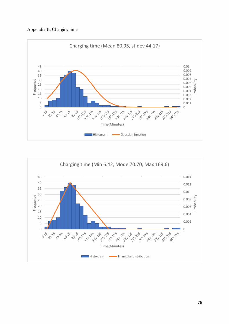
76

Appendix B: Charging time

0.00 50.00 100.00 150.00 200.00 250.00 300.00 350.00

00.0010.0020.0030.0040.0050.0060.0070.0080.0090.01

0

5

10

15

20

25

30

35

40

45

Astitel

Pro

bab

ility

Freq

uen

cy

Time(Minutes)

Charging time (Mean 80.95, st.dev 44.17)

Histogram Gaussian function

0 50 100 150 200 250 300 350

0

0.002

0.004

0.006

0.008

0.01

0.012

0.014

0

5

10

15

20

25

30

35

40

45

Pro

bab

ility

Freq

uen

cy

Time(Minutes)

Charging time (Min 6.42, Mode 70.70, Max 169.6)

Histogram Triangular distribution

77

Appendix C: Washing time

0.00 10.00 20.00 30.00 40.00 50.00 60.00 70.00

0

0.005

0.01

0.015

0.02

0.025

0.03

0

2

4

6

8

10

12

14

0-5 5-10 10-15 15-20 20-25 25-30 30-35 35-40 40-45 45-50 50-55 55-60 70-75

Pro

bab

ility

Freq

uen

cy

Time(Minutes)

Washing (Mean 22.75, st.dev 15.46)

Histogram Gaussian function

0 5 10 15 20 25 30 35 40 45 50 55 60 65 70 75

0

0.005

0.01

0.015

0.02

0.025

0.03

0.035

0

2

4

6

8

10

12

14

0-5 5-10 10-15 15-20 20-25 25-30 30-35 35-40 40-45 45-50 50-55 55-60 70-75 75-80

Freq

uen

cy

Time(Minutes)

Washing (Min, 1.05, Mode 13.07, Max 70.80)

Histogram Triangular distribution

78

Appendix D: Scaling time

0 20 40 60 80 100 120 140 160 180 200 220 240 260 280 300 320 340 360 380 400

0

0.002

0.004

0.006

0.008

0.01

0.012

0.014

0

2

4

6

8

10

12

14

Freq

uen

cy

Time(Minutes)

Scaling (Min 47.85, Mode 86.85, Max 200.62)

Histogram Triangular distribution

0 20 40 60 80 100 120 140 160 180 200 220 240 260 280 300 320 340 360 380 400

00.0010.0020.0030.0040.0050.006

0

5

10

15

Freq

uen

cy

Time(Minutes)

Scaling (Mean 105.89, st.dev 75.45)

Histogram Gaussian function

0 20 40 60 80 100 120 140 160 180 200 220 240 260 280 300 320 340 360 380 400

0

0.01

0.02

0.03

0.04

02468

101214

Freq

uen

cy

Time(Minutes)

Face scaling (Min 5.80, Mode 31.2, Max 57.67)

Histogram Triangular distribution

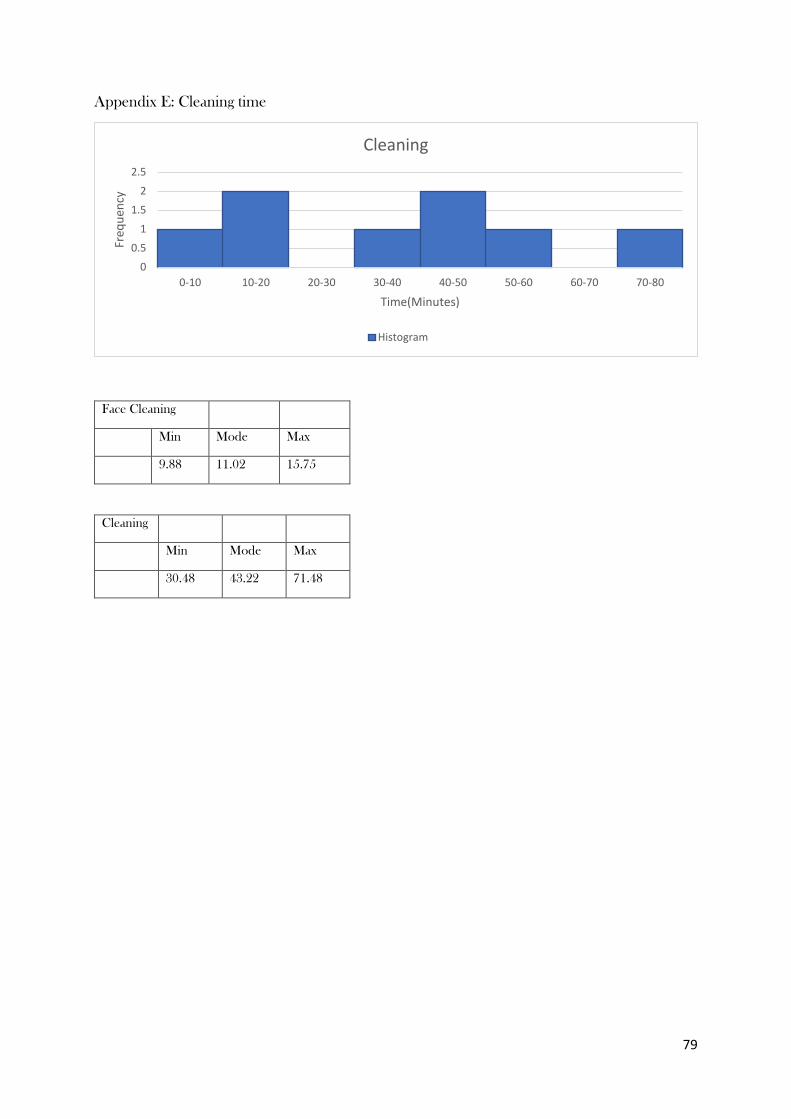
79

Appendix E: Cleaning time

Face Cleaning

Min Mode Max

9.88 11.02 15.75

Cleaning

Min Mode Max

30.48 43.22 71.48

0

0.5

1

1.5

2

2.5

0-10 10-20 20-30 30-40 40-50 50-60 60-70 70-80

Freq

uen

cy

Time(Minutes)

Cleaning

Histogram

80

Appendix F: Concrete spraying time

0 50 100 150 200 250

0

0.002

0.004

0.006

0.008

0.01

0.012

0

5

10

15

20

25

Pro

bab

ility

Freq

uen

cy

Time(Minutes)

Concrete (Min 4.48, Mode 44.43, Max 160.77)

Histogram Triangular distribution

0.00 50.00 100.00 150.00 200.00

0

0.001

0.002

0.003

0.004

0.005

0.006

0.007

0.008

0.009

0.01

0

5

10

15

20

25

Pro

bab

ility

Freq

uen

cy

Time(Minutes)

Concrete (Mean 66.22, st.dev 44.45)

Histogram Gaussian function

81

Appendix G: Bolting time

0.00 50.00 100.00 150.00 200.00 250.00

00.0010.0020.0030.0040.0050.0060.0070.008

0123456

0-1

0

20

-20

20

-30

30

-40

40

-50

50

-60

60

-70

70

-80

80

-90

90

-10

0

10

0-1

10

11

0-1

20

12

0-1

30

13

0-1

40

14

0-1

50

15

0-1

60

16

0-1

70

17

0-1

80

18

0-1

90

19

0-2

00

20

0-2

10

21

0-2

20

22

0-2

30

23

0-2

40

24

0-2

50

Pro

bab

ility

Freq

uen

cy

Time(Minutes)

Bolting drilling time (Mean 104.25, st.dev 56.61)

Histogram Gaussian function

0.00 100.00200.00300.00400.00500.00600.00700.00800.00900.001000.001100.001200.001300.001400.00

00.00050.0010.00150.002

010203040

5-5

5

55

-10

5

10

5-1

55

15

5-2

05

20

5-2

55

25

5-3

05

30

5-3

55

35

5-4

05

40

5-4

55

45

5-5

05

50

5-5

55

55

5-6

05

60

5-6

55

65

5-7

05

70

5-7

55

75

5-8

05

80

5-8

55

85

5-9

05

90

5-9

55

95

5-1

00

5

10

05

-10

55

10

55

-11

05

11

05

-11

55

11

55

-12

05

12

05

-12

55

13

05

-13

55

Astitel

Pro

bab

ility

Freq

uen

cy

Time(Minutes)

Total bolting time (Mean 325.15, st.dev 275.72)

Histogram Gaussian function

00.00050.0010.00150.0020.00250.0030.00350.0040.00450.005

02468

101214

5-1

5

45

-55

85

-95

12

5-1

35

16

5-1

75

20

5-2

15

24

5-2

55

28

5-2

95

32

5-3

35

36

5-3

75

40

5-4

15

44

5-4

55

48

5-4

95

52

5-5

35

56

5-5

75

60

5-6

15

64

5-6

55

68

5-6

95

72

5-7

35

76

5-7

75

80

5-8

15

84

5-8

55

94

5-9

55

98

5-9

95

10

45

-10

55

10

95

-11

05

11

35

-11

45

11

75

-11

85

12

15

-12

25

12

55

-12

65

12

95

-13

05

Total bolting time (Min 46.42, Mode 287.58, Max 485.18)

Pro

bab

ility

Freq

uen

cy

Time(Minutes)

Histogram Triangular distribution