Simulation Methods for the Characterization of Coiled-Tube ...

CTGH Simulation Methods 1 | 31

CTGH Simulation Methods

Simulation Methods for the Characterization of Coiled-Tube Gas Heaters

Andrew Greenop Per Peterson

UCBTH-16-003

December 2016 Department of Nuclear Engineering University of California, Berkeley

This research is being performed using funding received from the U.S. Department of Energy

Office of Nuclear Energy’s Nuclear Energy University Programs.


Contents Simulation Methods for the Characterization of Coiled-Tube Gas Heaters ........................... 1 Contents ......................................................................................................................................... 2 List of Figures ................................................................................................................................ 3 Acronyms and Abbreviations ...................................................................................................... 4 1 Introduction and Background on Coiled-Tube Gas Heaters ............................................. 5 2 THEEM 2.0: 0-D Analysis ..................................................................................................... 9

2.1 0-D Methodology .......................................................................................................................... 9 2.2 0-D Calculations ......................................................................................................................... 10

2.2.1 User Input and Thermodynamic Properties ........................................................................... 10 2.2.2 CTGH Geometry ................................................................................................................... 10 2.2.3 Gas Cross Flow Heat Transfer ............................................................................................... 12 2.2.4 Liquid Flow Heat Transfer .................................................................................................... 13 2.2.5 Surface Area Requirement ..................................................................................................... 13 2.2.6 Pressure Drops ....................................................................................................................... 14

3 THEEM 2.0: 2-D Simulation ............................................................................................... 16 3.1 Finite Volume Element Selection ............................................................................................. 17 3.2 Simulation Inputs ....................................................................................................................... 18 3.3 Simulation Calculations ............................................................................................................ 19

3.3.1 Thermodynamic & Heat Transfer Calculations ..................................................................... 19 3.3.2 Pressure Drop Calculations .................................................................................................... 22 3.3.3 Heat Exchanger Effectiveness Calculations .......................................................................... 24

3.4 Simulation Methodology ........................................................................................................... 25 3.5 THEEM 2-D Simulation Simplifying Assumptions ................................................................ 28

4 Conclusion and Future Work .............................................................................................. 30 5 References ............................................................................................................................. 31


List of Figures

Figure 1-1. Diagram of Mk1 PB-FHR coupled with RACC [1] .................................................... 5 Figure 1-2. CAD model of a Mk1 CTGH sub-bundle .................................................................... 7 Figure 1-3. CAD model of single full Mk1 CTGH ........................................................................ 7 Figure 1-4. Staggered tube arrangement of CTGH tube bundle ..................................................... 8 Figure 2-1. Location of overall heat transfer coefficient calculations in the 0-D model ................ 9 Figure 2-2. Definition of Geometric Variables in CTGH ............................................................. 11 Figure 3-1. THEEM 2-D Simulation Flowchart ........................................................................... 16 Figure 3-2. Example of a finite volume element .......................................................................... 17 Figure 3-3. Top view of radially sectioned Mk1 CTGH sub-bundle. ........................................... 18 Figure 3-4. Straight pipe vs. Curved Pipe Nusselt Numbers. ....................................................... 21 Figure 3-5. THEEM 2.0 Volume Element Selection Algorithm .................................................. 26 Figure 3-6. Example of a loop path for the simulation ................................................................. 27 Figure 3-7. Close-up of gaps in tube sub-bundle .......................................................................... 28

List of Tables

Table 1-1. MK1 RACC design parameters [2,3] ............................................................................ 6 Table 1-2. CTGHs Inlet & Outlet Design Parameters .................................................................... 8


Acronyms and Abbreviations

CAD – Computer Aided Design CTAH – Coiled tube air heater CTGH – Coiled tube gas heater FHR – Fluoride-salt-cooled, high-temperature reactor HP – High-pressure HRSG – Heat recovery steam generator LMTD - Log Mean Temperature Difference LP – Low-pressure LWR – Light water reactor Mk1 – Mark-1 PB-FHR – Pebble-bed fluoride-salt-cooled, high-temperature reactor PWR – Pressurized water reactor RACC – Reheat air-Brayton combined cycle SMR – Small Modular Reactor THEEM – Transverse Heat Exchange Effectiveness Model UCB – University of California, Berkeley


1 Introduction and Background on Coiled-Tube Gas Heaters The Coiled-Tube Gas Heater (CTGH) is a shell-and-tube heat exchanger designed to act as an interface between a liquid and gas. The ultimate goal for this heat exchanger is to be used with different liquid coolants and gas power conversion cycles, such as liquid sodium with a supercritical CO2 power conversion system. However, there is not a point design for this application yet. So, in order to develop a simulation for the CTGH, it was necessary to model based on an existing system design that uses the CTGH. For this reason, the Mark 1 Pebble Bed Fluoride Salt-Cooled High-Temperature Reactor (Mk1 PB-FHR) was used as the first application for the simulation. The Mk1 PB-FHR is one of the latest high temperature reactors and small modular reactor (SMR) designs [1]. Because the molten fluoride salt used as a coolant has a boiling temperature above 1400°C, the coolant remains single-phase during normal operation and transients. The resulting low operating pressure means the reactor can operate at a much higher temperature range than conventional Light Water Reactors (LWRs). The inlet temperature of the molten salt entering the Mk1 PB-FHR core is 600°C, where it is heated to an average outlet temperature of 700°C. However, this higher temperature range means that a conventional Rankine steam cycle would be less efficient for power conversion than it would for a LWR. For this reason, the Mk1 PB-FHR was designed to be coupled with the Mk1 Reheat Air-Brayton Combined Cycle (RACC) for power conversion. A diagram of the full Mk1 RACC coupled with the Mk1 PB-FHR is shown in Figure 1-1.

Figure 1-1. Diagram of Mk1 PB-FHR coupled with RACC [1]

In the baseline RACC shown in Figure 1-1, filtered air from the atmosphere is first run through a compressor. This high pressure air then flows through the High Pressure (HP) CTGH, which in


this case can be called a Coiled Tube Air Heater, or CTAH, where it is heated by molten salt from the FHR core. The air then enters Turbine 1 where it undergoes expansion. The air then enters the Low Pressure (LP) CTAH so that it can be reheated by molten salt from the core. The air flows into Turbine 2 where it is expanded to nearly atmospheric pressure and is sent to a heat recovery steam generator (HRSG). The design parameters for the Mk1 RACC are given in Table 1-1. To further increase power output, natural gas can be injected and co-fired downstream of the second CTAH [1]. So, in order for this RACC to work efficiently, the CTAHs need to be effective interfaces for heat transfer between the air and the molten salt.

Table 1-1. Mk1 RACC design parameters [2,3]

Component Temperature [°C] Pressure [bar] Compressor Inlet (atmosphere) 15.00 1.013

Compressor Outlet 418.6 18.76 HP CTAH Outlet 670.0 ~18.701 Turbine 1 Outlet 418.6 4.99 LP CTAH Outlet 670.0 ~4.751

Since the FHR is an SMR, one of the major design goals is to minimize the size of major components to enable rail transportability. For this reason, the Mk1 CTGH uses a spiral geometry for the tubes to minimize the total volume of the heat exchanger while maximizing the heat transfer surface area between the liquid and gas. The tube-side salt flows into the top of the Mk1 CTGH through four inlet manifold pipes. As the molten salt flows down the manifold pipes, it can be distributed to one of the 36 tube sub-bundles. These sub-bundles are stacked on top of each other, separated by spacer plates. Figure 1-2 shows a CAD model of a Mk1 sub-bundle, and Figure 1-3 shows a CAD model of the full Mk1 CTGH2. In each of the sub-bundles, the molten salt flows inward through multiple small tubes in a sloped, spiral pattern until it reaches one of the four inner manifold pipes. The salt then flows through these pipes until it exits the CTGH through the bottom of the heat exchanger. For the shell side, high or low pressure air enters through the bottom of the CTGH and flows upward through the center of the sub-bundles and then radially outward through the spiral tube bundles, which are arranged in a staggered pattern, as shown in Figure 1-4. The air then flows upward through the outer annulus of the pressure vessel until it exits the top of the CTGH. Using this arrangement, the CTGH acts essentially as a counterflow heat exchanger. The hot salt inlet heats the hot air that is leaving the CTGH bundle, and the cold salt that is exiting the tubes heats the cold air entering the bundle. This means that the temperature difference between the salt and air remains relatively small across the heat exchanger improving overall heat transfer for the CTGH.

1 CTAH outlet pressures are based on a rough estimate of head loss of the air flowing through the CTAH. 2 All CAD models were created using SOLIDWORKS.


Figure 1-2. CAD model of a Mk1 CTGH sub-bundle

Figure 1-3. CAD model of single full Mk1 CTGH


Figure 1-4. Staggered tube arrangement of CTGH tube bundle3

The nominal parameters based on the designs of the Mk1 PB-FHR and the RACC are given in Table 1-2.

Table 1-2. CTGHs Inlet & Outlet Design Parameters

Parameters Salt Air Inlet Temperature [°C] 700 418.6

Inlet Pressure (HP/LP) [bar] ~3.0/~3.04 18.76/4.99 Mass Flow Rate [kg/s] 418.5 480.2

Outlet Temperature [°C] 600 670 With these parameters, it is assumed that CTGH has an effectiveness of 0.9 to produce the given outlet temperatures. A finite volume computer code, called the Transverse Heat Exchange Effectiveness Model (THEEM), was developed in MATLAB to analytically predict the approximate effectiveness of one of the CTGH sub-bundles, subject to simplifying assumptions about the flow distribution that will be studied in future versions of the code. THEEM 1.0 was developed based on a 0-D analysis of the heat transfer for the CTGH created in excel. THEEM 1.0 started out as a 2-D simulation that could calculate the heat transfer and temperature distribution that occurs across a single tube sub-bundle. The 2-D simulation also can calculate the pressure distribution for both the air and molten salt that flows through the sub-bundle. THEEM 2.0 expands on THEEM 1.0 by removing many of the simplifying assumptions and also including a 0-D analysis performed in MATLAB. Both the 0-D and 2-D codes will be discussed in more detail in the following sections of this paper.

3 The solid red tubes represent the heating elements that prevent salt freezing in the CTGH during shutdowns and other anticipated occupational occurrences. 4 The salt inlet pressure is only an approximation based on the expected salt head loss in the CTGH.


2 THEEM 2.0: 0-D Analysis

2.1 0-D Methodology

The 0-D model works by calculating the total heat transfer area for the tube bundle and then calculating the average heat transfer properties at a single point in the center of the bundle. The 0-D analysis uses similar inputs as the 2-D simulation, but it assumes the values for the outlet temperatures and overall heat transfer for the gas and liquid. It then calculates the overall heat transfer coefficient, 𝑈𝑈, by treating the CTGH as a simple cross flow heat exchanger with fully developed flow. It calculates the properties at the mean of the inlet and outlet temperatures for the gas and liquid, respectively. Also, for the gas flow through the tube bundle, it uses a flow area based on the diameter of the bundle halfway between the inside diameter and outside diameter of the bundle. Figure 2-1 highlights this location. Finally, the total tube surface area, A, is calculated for the entire CTGH tube bundle. The total heat transfer can then be calculated using the log mean temperature difference (LMTD) formula:

𝑄𝑄!"! = 𝐹𝐹 ∗ 𝑈𝑈𝑈𝑈 ∗ ∆𝑇𝑇!"#$ # 1 Here ∆𝑇𝑇!"#$ is the log-mean temperature difference, and F is the F-factor of the heat exchanger, the ratio of the actual heat transfer to the heat transfer possible if this was an ideal counterflow heat exchanger. This represents how close the heat exchanger functions to an actual counterflow heat exchanger. The 0-D analysis can quickly show how changing certain aspects of the geometry, or even the point design, can affect the overall heat transfer area and/or the F-factor.

Figure 2-1. Location of overall heat transfer coefficient calculations in the 0-D model

The F-factor corrects for the actual flow distribution in bundle, as opposed to perfect counter-flow, and is calculated using 2-D and 3-D bundle calculations. The 0-D model then provides the


capability to rapidly calculate and optimize the performance of bundle designs with different surface areas (numbers and lengths of tubes) and other design parameters. This model is relatively flexible when it comes to working with different heat transfer fluids. The thermodynamic properties of the liquid and gas are obtained from functions with their properties based on the temperatures and pressure of the liquid and the gas. Using these functions means that the 0-D code can work with different fluids and can choose which functions to use based on the user input. Also, the user input and geometrical calculations based on these inputs make it easy to modify the geometry of the CTGH. When a desirable 0-D design is identified, the 3-D model can be used to verify the correct value of the F-factor.

2.2 0-D Calculations

2.2.1 User Input and Thermodynamic Properties The first section of the 0-D code imports an input file with various input variables defined by the user. The user gives both geometrical parameters of the CTGH and the inlet conditions of the liquid and gas. For the geometry, the user defines the outside diameter of each tube (𝐷𝐷!), the thickness of those tubes (𝑡𝑡), the tube material, the transverse, or vertical, pitch-to-diameter ratio of the tubes in the bundle (𝑆𝑆!), the longitudinal, or radial, pitch-to-diameter ratio of the tubes in the bundle (𝑆𝑆!), and the number of liquid manifold inlets (𝑁𝑁!!!"#$%&'). For both the liquid and gas inlet conditions, the user defines the mass flow rates (𝑚𝑚! & 𝑚𝑚!), the inlet pressures (𝑃𝑃!,! & 𝑃𝑃!,!), and the inlet temperatures (𝑇𝑇!,! & 𝑇𝑇!,!). The user also chooses the type of liquid and gas that is being used. Then, the user must give the outlet temperatures for both the gas and the liquid (𝑇𝑇!,! & 𝑇𝑇!,!). After loading the variables from the input file, the program calculates the average temperatures of both the liquid and the gas based on their inlet and outlet temperatures (𝑇𝑇!,!"# & 𝑇𝑇!,!"#). It also calculates the LMTD:

∆𝑻𝑻𝑳𝑳𝑳𝑳𝑳𝑳𝑳𝑳 =𝑻𝑻𝒍𝒍,𝒐𝒐−𝑻𝑻𝒈𝒈,𝒊𝒊 − 𝑻𝑻𝒍𝒍,𝒊𝒊−𝑻𝑻𝒈𝒈,𝒐𝒐

𝒍𝒍𝒍𝒍𝑻𝑻𝒍𝒍,𝒐𝒐−𝑻𝑻𝒈𝒈,𝒊𝒊𝑻𝑻𝒍𝒍,𝒊𝒊−𝑻𝑻𝒈𝒈,𝒐𝒐

# 2

The program then calls a function to obtain the thermodynamic properties for the liquid and another function to obtain the properties for the gas. The program selects which functions to run based on the user’s selection of gas and liquid. The input for the gas function is the inlet pressure and the average temperature of the gas. The input for the liquid function is the average temperature of the liquid. Finally, this section defines the properties of the tube material based on the user’s material selection. For the 0-D model, the only property needed for the tube material is the thermal conductivity.

2.2.2 CTGH Geometry This section of the code determines the geometry of the bundle. First, the code specifies the number of sub-bundles (𝑁𝑁!"#$%&'), the thickness of the spacer disk (𝑡𝑡!"#$), the number of tube rows per layer leaving each manifold (𝑁𝑁!"#$), the number of tube layers per sub-bundle (𝑁𝑁!"#$%&), the number of tubes replaced by a heater rod in each layer (𝑁𝑁!!"#$%&), the inside diameter of the tube bank (𝐷𝐷!",!"#$), the number of times each tube loops around the center


(𝑁𝑁!""#$), the number of tie rod gaps (𝑁𝑁!"#$), and the width of each tie rod gap (𝑡𝑡!"#). Figure 2-2 shows the difference between tube rows and tube layers along with the difference between the transverse and longitudinal pitches using the CAD model shown in Figure 1-4. Given this information and the geometrical data given by the user input, the code then calculates the total number of tubes in the bundle, excluding the heater rods:

𝑵𝑵𝒕𝒕𝒕𝒕𝒕𝒕𝒕𝒕𝒕𝒕 = 𝑵𝑵𝒃𝒃𝒃𝒃𝒃𝒃𝒃𝒃𝒃𝒃𝒃𝒃𝒃𝒃 ∗𝑵𝑵𝑴𝑴𝑴𝑴𝑴𝑴𝑴𝑴𝑴𝑴𝑴𝑴𝑴𝑴𝑴𝑴𝑴𝑴 ∗𝑵𝑵𝒍𝒍𝒍𝒍𝒍𝒍𝒍𝒍𝒍𝒍𝒍𝒍 ∗ 𝑵𝑵𝒓𝒓𝒓𝒓𝒓𝒓𝒓𝒓 −𝑵𝑵𝒉𝒉𝒉𝒉𝒉𝒉𝒉𝒉𝒉𝒉𝒉𝒉𝒉𝒉 # 3

Figure 2-2. Definition of Geometric Variables in CTGH

Next, it calculates the number of vertical tube rows, including actual tubes and heater rods, in the radial direction:

𝑵𝑵𝑳𝑳 = 𝟐𝟐 ∗𝑵𝑵𝑴𝑴𝑴𝑴𝑴𝑴𝑴𝑴𝑴𝑴𝑴𝑴𝑴𝑴𝑴𝑴𝑴𝑴 ∗𝑵𝑵𝒍𝒍𝒍𝒍𝒍𝒍𝒍𝒍𝒍𝒍 ∗𝑵𝑵𝒓𝒓𝒓𝒓𝒓𝒓𝒓𝒓 # 4

Since the layers are staggered, a factor of 2 is needed to include the tube rows that correspond to the staggered layers. Then, based on the number of vertical tube rows and the tie rod gaps, it calculates the total width of the tube bank:

𝒕𝒕𝒃𝒃𝒃𝒃𝒃𝒃𝒃𝒃 = 𝑵𝑵𝑳𝑳 ∗ 𝑺𝑺𝑳𝑳 ∗𝑫𝑫𝒐𝒐 +𝑵𝑵𝒈𝒈𝒈𝒈𝒈𝒈𝒈𝒈 ∗ 𝒕𝒕𝒈𝒈𝒈𝒈𝒈𝒈 # 5

Using the total bank width and the inside diameter of the bundle, the code calculates the outer diameter of the bundle and the diameter at the middle of the bundle, which is highlighted in Figure 2-1:

𝑫𝑫𝒐𝒐𝒐𝒐𝒐𝒐,𝒃𝒃𝒃𝒃𝒃𝒃𝒃𝒃 = 𝑫𝑫𝒊𝒊𝒊𝒊,𝒃𝒃𝒃𝒃𝒃𝒃𝒃𝒃 + 𝟐𝟐 ∗ 𝒕𝒕𝒃𝒃𝒃𝒃𝒃𝒃𝒃𝒃 # 6

𝑫𝑫𝒂𝒂𝒂𝒂𝒂𝒂,𝒃𝒃𝒃𝒃𝒏𝒏𝒌𝒌 =𝑫𝑫𝒊𝒊𝒊𝒊,𝒃𝒃𝒃𝒃𝒃𝒃𝒃𝒃 +𝑫𝑫𝒐𝒐𝒐𝒐𝒐𝒐,𝒃𝒃𝒃𝒃𝒃𝒃𝒃𝒃

𝟐𝟐 # 7

SL

ST

Tube Rows

Tube Layer


The code then calculates the height of each sub-bundle in the vertical direction, not including the spacer disk between each bundle:

𝑯𝑯𝒃𝒃𝒃𝒃𝒃𝒃𝒃𝒃𝒃𝒃𝒃𝒃 = 𝑫𝑫𝒐𝒐 ∗ 𝑺𝑺𝑻𝑻 ∗𝑵𝑵𝒍𝒍𝒍𝒍𝒍𝒍𝒍𝒍𝒍𝒍𝒍𝒍 + 𝟏𝟏

𝟐𝟐 # 8

Next, it finds the total height of the bundle, including the spacer disks: 𝑯𝑯𝒃𝒃𝒃𝒃𝒃𝒃𝒃𝒃 = 𝑵𝑵𝒃𝒃𝒃𝒃𝒃𝒃𝒃𝒃𝒃𝒃𝒃𝒃𝒃𝒃 ∗ 𝑯𝑯𝒃𝒃𝒃𝒃𝒃𝒃𝒃𝒃𝒃𝒃𝒃𝒃 + 𝒕𝒕𝒅𝒅𝒅𝒅𝒅𝒅𝒅𝒅 # 9

Then, it is possible to find the average overall flow area for the gas through the bundle, which corresponds to the flow area at the radial location highlighted in Figure 2-1:

𝐴𝐴!"#$,!"# = 𝜋𝜋 ∗ 𝐷𝐷!"#,!"#$ ∗ 𝐻𝐻!"#$ − 𝑡𝑡!"#$ ∗ 𝑁𝑁!"#$%&' # 10

Finally, this section of the code calculates the average tube length by multiplying the circumference of the radial center of the tube bundle by the number of times each tube loops around the bundle. Then, it uses that length along with the total number of tubes to calculate the overall surface area for heat transfer between the gas and the liquid in the bundle.

𝑳𝑳𝒕𝒕𝒕𝒕𝒃𝒃𝒃𝒃 = 𝑵𝑵𝒍𝒍𝒍𝒍𝒍𝒍𝒍𝒍𝒍𝒍 ∗ 𝝅𝝅 ∗𝑫𝑫𝒂𝒂𝒂𝒂𝒂𝒂,𝒃𝒃𝒃𝒃𝒃𝒃𝒃𝒃 # 11

𝑨𝑨𝒔𝒔𝒖𝒖𝒖𝒖𝒖𝒖 = 𝑵𝑵𝒕𝒕𝒕𝒕𝒕𝒕𝒕𝒕𝒕𝒕 ∗ 𝝅𝝅 ∗𝑫𝑫𝒐𝒐 ∗ 𝑳𝑳𝒕𝒕𝒕𝒕𝒕𝒕𝒕𝒕 # 12

2.2.3 Gas Cross Flow Heat Transfer The next section of the code calculates the heat transfer coefficient of the gas. The code uses the area at the radial center of the bundle, which is the height of the bundle multiplied by the average diameter of the sub-bundle, as the cross flow area for the gas flow. This location is highlighted in Figure 2-1. It uses this area and the pitch-to-diameter ratios to calculate the maximum velocity of the gas and its Reynolds number. For the CTAH in the Mk1 PB-FHR, the code uses the Grimson Correlation, which calculates the heat transfer coefficient for gas flowing over tube bundles using the following Nusselt number correlation:

𝑵𝑵𝑵𝑵𝒈𝒈 = 𝑪𝑪𝟏𝟏𝑹𝑹𝑹𝑹𝒈𝒈,𝒎𝒎𝒎𝒎𝒎𝒎𝒎𝒎 # 13

This correlation is used when there are more than 10 tube rows, so that the gas flow is fully developed in the tube bundles. It also corresponds to the following range of Reynolds numbers: 2,000 < 𝑅𝑅𝑅𝑅!,!"# < 40,000. This correlation is also used only for air; therefore, it is only valid for Pr = 0.7. 𝐶𝐶! and 𝑚𝑚 are found using empirically derived tables given by Incropera et al. [4]. Their values depend on the transverse and longitudinal pitch-to-diameter ratios for the bundle. In Equation 12, 𝑅𝑅𝑅𝑅!,!"# refers to the Reynolds number calculated using the maximum velocity of the air flowing radially through the tube bundle. This corresponds to the gas flowing through the smallest cross sectional area between the pipes. The Reynolds number is given by:

𝑹𝑹𝑹𝑹𝒈𝒈,𝒎𝒎𝒎𝒎𝒎𝒎 =𝝆𝝆𝒈𝒈𝑫𝑫𝒐𝒐𝒗𝒗𝒎𝒎𝒎𝒎𝒎𝒎

𝝁𝝁𝒈𝒈 # 14

𝐷𝐷! is the outer diameter of the tubes, 𝜌𝜌!, the density of the gas, and 𝜇𝜇!, the dynamic viscosity of the gas. The maximum velocity, 𝑣𝑣!"#, is found by multiplying the average velocity of the gas


by the ratio of the total gas flow area of the tube bundle by the smallest flow area between the tubes. In order to reduce anisotropic gas flow, the tubes are arranged as close as possible to an equilateral pitch pattern, which affects the ratio of flow areas. In this arrangement, the equation for maximum velocity is:

𝒗𝒗𝒎𝒎𝒎𝒎𝒎𝒎 = 𝒗𝒗𝒂𝒂𝒂𝒂𝒂𝒂𝑺𝑺𝑻𝑻

𝑺𝑺𝑻𝑻 − 𝟏𝟏 # 15

The average velocity, 𝑣𝑣!"#, is based on the mass flow of the gas, 𝑚𝑚!, and the overall gas flow area, 𝐴𝐴!"#$,!"#:

𝒗𝒗𝒂𝒂𝒂𝒂𝒂𝒂 =𝒎𝒎𝒈𝒈

𝝆𝝆𝒈𝒈𝑨𝑨𝒇𝒇𝒇𝒇𝒇𝒇𝒇𝒇,𝒂𝒂𝒂𝒂𝒂𝒂 # 16

After calculating the Nusselt number, it is possible to find the convection heat transfer coefficient for the gas using the definition of the Nusselt number and the thermal conductivity of the gas. The convection heat transfer coefficient is then used to find the thermal resistivity of the gas.

𝒉𝒉𝒈𝒈 =𝑵𝑵𝑵𝑵𝒈𝒈 ∗ 𝒌𝒌𝒈𝒈

𝑫𝑫𝒐𝒐 # 17

𝑹𝑹𝒈𝒈 =𝟏𝟏𝒉𝒉𝒈𝒈 # 18

2.2.4 Liquid Flow Heat Transfer For the liquid flowing through the tubes, the 0-D code uses a straight pipe Nusselt number correlation. It uses the correlation for fully developed laminar flow with a constant wall temperature:

𝑵𝑵𝑵𝑵𝒍𝒍 = 𝟑𝟑.𝟔𝟔𝟔𝟔 # 19

Similar to Section 2.2.3, the Nusselt number is used to find the convection heat transfer coefficient for the liquid along with its thermal resistivity:

𝒉𝒉𝒍𝒍 =𝑵𝑵𝑵𝑵𝒍𝒍 ∗ 𝒌𝒌𝒍𝒍𝑫𝑫𝒊𝒊

# 20

𝑹𝑹𝒍𝒍 =𝑫𝑫𝒐𝒐

𝑫𝑫𝒊𝒊∗𝟏𝟏𝒉𝒉𝒍𝒍 # 21

2.2.5 Surface Area Requirement First, this section calculates the desired heat transfer based on the gas inlet and outlet temperatures, the gas heat capacitance, 𝐶𝐶!!, and the gas mass flow rate:

𝑸𝑸 =𝒎𝒎𝒈𝒈𝑪𝑪𝒑𝒑𝒈𝒈 𝑻𝑻𝒈𝒈,𝒐𝒐 − 𝑻𝑻𝒈𝒈,𝒊𝒊 # 22

Using this desired heat transfer rate, the code then finds the surface area required to obtain this rate assuming that the heat exchanger is a perfect counterflow heat exchanger with a counterflow correction factor of F=1.0:


𝑨𝑨𝒊𝒊𝒊𝒊𝒊𝒊𝒊𝒊𝒊𝒊 =𝑸𝑸

𝑼𝑼 ∗ ∆𝑻𝑻𝑳𝑳𝑳𝑳𝑳𝑳𝑳𝑳 # 23

The overall heat transfer coefficient, 𝑈𝑈, is found using the liquid and gas heat transfer coefficients found from the thermal resistivity formulas in Equations 17 and 20 along with the thermal resistivity of the tube wall:

𝑅𝑅! = 𝑙𝑙𝑙𝑙 !!!!

∗ !!!∗!!

# 24 In this equation, 𝑘𝑘! is the thermal conductivity of the tube wall. Using these three values for resistivity, the code then calculates overall heat transfer coefficient:

𝑼𝑼 =𝟏𝟏

𝑹𝑹𝒍𝒍 + 𝑹𝑹𝒕𝒕 + 𝑹𝑹𝒈𝒈 # 25

It then calculates the minimum F-factor required to obtain the desired heat transfer. It does this by taking the ratio between the ideal counterflow heat exchanger surface area and the actual surface area:

𝑭𝑭𝒎𝒎𝒎𝒎𝒎𝒎 =𝑨𝑨𝒊𝒊𝒊𝒊𝒊𝒊𝒊𝒊𝒊𝒊𝑨𝑨𝒔𝒔𝒔𝒔𝒔𝒔𝒔𝒔

# 26

If 𝐹𝐹!"# is greater than 1, then it is impossible for this heat exchanger geometry to obtain the desired heat transfer given the liquid and gas inlet and outlet conditions. Next, in order to calculate the effectiveness of the heat exchanger, the 0-D model uses the following formula:

𝜺𝜺 =𝑸𝑸

𝑸𝑸𝒎𝒎𝒎𝒎𝒎𝒎 # 27

𝑄𝑄!"# is the maximum heat transfer possible for the heat exchanger given its inlet conditions: 𝑸𝑸𝒎𝒎𝒎𝒎𝒎𝒎 = 𝑪𝑪𝒎𝒎𝒎𝒎𝒎𝒎 𝑻𝑻𝒍𝒍,𝒊𝒊 − 𝑻𝑻𝒈𝒈,𝒊𝒊 # 28

𝑪𝑪𝒎𝒎𝒎𝒎𝒎𝒎 =𝒎𝒎𝒎𝒎𝒎𝒎 𝒎𝒎𝒍𝒍𝑪𝑪𝒑𝒑𝒍𝒍, 𝒎𝒎𝒈𝒈𝑪𝑪𝒑𝒑𝒈𝒈 # 29

2.2.6 Pressure Drops This final section of the code calculates the overall pressure drop of the liquid and the gas across the CTGH bundle. For the gas pressure drop, it uses the Zukauskas correlation [4] for a gas flowing through a staggered tube bundle:

∆𝑷𝑷𝒈𝒈 = 𝒇𝒇 𝒈𝒈 ∗ 𝝌𝝌 ∗ 𝑵𝑵𝑳𝑳 ∗𝝆𝝆𝒈𝒈 ∗ 𝒗𝒗𝒎𝒎𝒎𝒎𝒎𝒎𝟐𝟐

𝟐𝟐 # 30

In this correlation, the friction factor, 𝑓𝑓 !, and the correction factor, 𝜒𝜒, are found using empirical charts in Incropera et al. [4]. These values are based on the gas Reynolds number along with the tube pitch-to-diameter ratios, 𝑆𝑆! and 𝑆𝑆!. 𝑁𝑁! is the number of tube rows that the gas must pass through, which is given by the CTGH geometry section of the code. 𝑣𝑣!"# refers to the maximum gas velocity calculated in Section 2.2.3.


For the liquid pressure drop, since it is liquid flowing through a pipe, the Darcy-Weisbach equation is used to measure the frictional pressure loss from flow through the pipe:

∆𝑷𝑷𝒍𝒍 = 𝒇𝒇𝒍𝒍 ∗𝑳𝑳𝒕𝒕𝒕𝒕𝒕𝒕𝒕𝒕𝑫𝑫𝒊𝒊𝒊𝒊𝒊𝒊𝒊𝒊𝒊𝒊

∗ 𝝆𝝆𝒍𝒍 ∗𝒖𝒖𝒍𝒍𝟐𝟐

𝟐𝟐 # 31

In this equation, the fluid is assumed to be laminar and, like the heat transfer coefficient calculation, the tube is treated as if it was straight. For this reason, a laminar, straight pipe correlation is used for the friction factor:

𝒇𝒇𝒍𝒍 =𝟔𝟔𝟔𝟔𝑹𝑹𝑹𝑹𝒍𝒍

# 32

𝑹𝑹𝑹𝑹𝒍𝒍 =𝝆𝝆𝒍𝒍𝒖𝒖𝒍𝒍𝑫𝑫𝒊𝒊

𝝁𝝁𝒍𝒍 # 33

In Equations 31 and 33, 𝐿𝐿!"#$ is the average length of the tubes in the CTGH bundle, 𝐷𝐷! the inside diameter of those tubes, 𝜌𝜌! the density of the liquid, 𝜇𝜇! the dynamic viscosity of the liquid, and 𝑢𝑢! the average velocity of the liquid flowing through the pipes based on the average liquid mass flow rate through each tube and the cross-sectional flow area of each tube. After all of these calculations are performed, the code then saves all of the variables to an output file.


3 THEEM 2.0: 2-D Simulation

Figure 3-1. THEEM 2-D Simulation Flowchart


THEEM 1.0 was originally written as a 2-D simulation code. The code performs a finite volume simulation on a 2-D cross section of one of the sub-bundles. The simulation then calculates the effectiveness of the sub-bundle, the total heat transfer, the heat transfer distribution, and the temperature and pressure distribution of the liquid and gas across the sub-bundle. This section explains how the 2-D simulation was originally developed for THEEM 1.0 along with how the code was updated to version 2.0 to reduce many of the assumptions made in version 1.0. A flowchart summarizing how the 2-D simulation works is shown in Figure 3-1.

3.1 Finite Volume Element Selection

To perform a finite volume simulation, the first step is to determine the size and geometry of the finite volume element that will be used in the calculations. The first constraint is to make the volume elements small while still being able to model the geometry of the tube bundle. The next constraint is that the volume elements needed to be close to cubic in shape to simplify the geometry. There also needs to be few if any partial volume elements. In other words, the volume elements’ geometries need to be consistent across an entire sub-bundle in order to simplify the calculations. Ideally, one volume element can be used to section the entire CTGH. For example, because each of the sub-bundles in the original Mk1 design is made up of 20 radial layers, the number of vertical rows in the geometry should be a factor of 20. Also, because the original Mk1 design has 60 tube rows in the radial direction, the number of rows in the volume element needs to be a factor of 60. Therefore, in order to meet these constraints while maintaining the overall sense of the tube bundle geometry, it is determined that the volume for the original Mk1 design should have 5 layers and 5 vertical rows. Then, in order to cut the volumes azimuthally, the CTGH was sectioned evenly so that the volumes were approximately cubic in shape. Figure 3-2 shows a typical volume element. This method of sectioning the sub-bundle into approximately equal finite volume elements meant that, in the original Mk1 design, there were four rows of volume elements vertically, 12 rows radially, and 108 sections azimuthally for each sub-bundle. Figure 3-3 shows a top view of the radially sectioned sub-bundle.

Figure 3-2. Example of a finite volume element

Gas

Liquid

Gas


Figure 3-3. Top view of radially sectioned Mk1 CTGH sub-bundle.

The general geometry is the same for each of these volumes. However, the dimensions can change depending on the radial position in the grid. The height of each volume and the width of each volume in the radial direction remains constant despite the position of the volume in the grid. Even though the tubes spiraled downward, they all sloped down at the same angle. So, the volume elements have the same number of tubes with the same spacing and same height. These dimensions change based solely on the pitch of the tube bundle and the diameter of the tubes. However, the length of the volume in the azimuthal direction changes based on the row number in the radial direction. The THEEM code takes this into account by increasing the azimuthal length of each volume element as its radial distance from the center of the CTGH sub-bundle increases.

3.2 Simulation Inputs

One of the ultimate goals of the THEEM development effort is to introduce an optimization capability that will find the geometry that gives high heat transfer effectiveness, while minimizing the overall heat transfer volume. This means that certain parameters of the CTGH model need to be easily adjustable. When the 2-D simulation is initialized, the MATLAB program asks for the following inputs for the CTGH geometry: (i) the outer diameter of each tube (𝐷𝐷!), (ii) the wall thickness of these tubes (𝑡𝑡), (iii) the longitudinal pitch-to-diameter ratio of the tubes in the bundle (𝑆𝑆!), (iv) the transverse pitch-to-diameter ratio for the tubes (𝑆𝑆!), and (v) the number of inlets for the CTGH (𝑁𝑁!"#$%&'()). The number of inlets refers to the number of liquid manifold pipes feeding each sub-bundle. The Mk1 CTGH has 4 manifold pipes, as seen in Figure 1-2 and Figure 1-3, but modifying the number of inlets can affect the overall effectiveness, thus, the number of inlets is classified as an input variable. The 2-D THEEM model is also designed to simulate different fluids with variable inlet conditions, like the 0-D MATLAB code. The 2-D simulation requires the user to specify the


type of gas and liquid flowing through the heat exchanger, the tube material, and the inlet conditions of the gas and liquid. The required inlet conditions are the inlet temperatures (𝑇𝑇!,!" & 𝑇𝑇!,!"), the inlet pressures (𝑃𝑃!,!" & 𝑃𝑃!,!"), and the mass flow rates for each fluid (𝑚𝑚! & 𝑚𝑚!).

3.3 Simulation Calculations

Using the program inputs from Section 3.2, it is possible to determine total heat transfer as well as the temperature and pressure distributions of the liquid and gas across the CTGH sub-bundle. This section describes the calculations that the code performs to obtain this information. Many of these formulas are similar to the 0-D calculations. However, these calculations are used for a single finite volume element instead of the entire CTGH tube bundle. This section also highlights and explains why some correlations used in the 2-D code are different from the 0-D version.

3.3.1 Thermodynamic & Heat Transfer Calculations In order to find the heat transfer as well as the temperature of the gas and fluid flowing out of each volume, the following equations were used for each control volume:

𝑸𝑸𝒊𝒊,𝒋𝒋 =𝒎𝒎𝒍𝒍𝑪𝑪𝒑𝒑𝒍𝒍 𝑻𝑻𝒍𝒍𝒊𝒊,𝒋𝒋 − 𝑻𝑻𝒍𝒍𝒊𝒊,𝒋𝒋!𝟏𝟏 # 34

𝑸𝑸𝒊𝒊,𝒋𝒋 =𝒎𝒎𝒈𝒈𝑪𝑪𝒑𝒑𝒈𝒈 𝑻𝑻𝒈𝒈𝒊𝒊!𝟏𝟏,𝒋𝒋 − 𝑻𝑻𝒈𝒈𝒊𝒊,𝒋𝒋 # 35

𝑸𝑸𝒊𝒊,𝒋𝒋 = 𝑼𝑼𝑼𝑼𝒊𝒊,𝒋𝒋 ∗𝑻𝑻𝒍𝒍𝒊𝒊,𝒋𝒋 + 𝑻𝑻𝒍𝒍𝒊𝒊,𝒋𝒋!𝟏𝟏

𝟐𝟐−𝑻𝑻𝒈𝒈𝒊𝒊,𝒋𝒋 + 𝑻𝑻𝒈𝒈𝒊𝒊!𝟏𝟏,𝒋𝒋

𝟐𝟐# 36

where 𝑄𝑄!,!is the heat transfer that occurs in the volume cell and 𝑈𝑈𝑈𝑈!,! is the overall heat transfer coefficient multiplied by the surface area of the tubes in the volume. These 3 equations have 3 unknowns: (i) the outlet temperatures of the gas, 𝑇𝑇!!!!,!, (ii) the outlet temperature of the liquid, 𝑇𝑇!!,!!!, and (iii) the heat transfer rate, 𝑄𝑄!,!. The inlet temperatures are either the inlet temperatures for the CTGH or the previous volume’s outlet temperatures. The gas volume’s mass flow rates are calculated by evenly dividing the overall mass flow rates over each of the volume cells. The liquid mass flow rate is calculated by evenly dividing the flow rate between each sub-bundle and each manifold inlet. The heat capacities are temperature dependent properties of the liquid or gas. 𝑈𝑈𝑈𝑈!,! can be calculated based on thermodynamic and fluid properties of the tube bundle in the volume element. For each volume element, the overall heat transfer coefficient, 𝑈𝑈𝑈𝑈, is calculated given the thermal resistance of the liquid in the tube, 𝑅𝑅!"#, of the tube wall, 𝑅𝑅!"#$, and of the gas outside of the tubes, 𝑅𝑅!"#:

𝑼𝑼𝑼𝑼 =𝟏𝟏

𝑹𝑹𝒍𝒍𝒍𝒍𝒍𝒍 + 𝑹𝑹𝒕𝒕𝒕𝒕𝒕𝒕𝒕𝒕 + 𝑹𝑹𝒈𝒈𝒈𝒈𝒈𝒈 # 37

The thermal resistivity of the liquid, 𝑅𝑅!"#, is:


𝑹𝑹𝒍𝒍𝒍𝒍𝒍𝒍 =𝟏𝟏

𝒉𝒉𝒍𝒍 ∗ 𝒏𝒏𝒕𝒕,𝒗𝒗𝒗𝒗𝒗𝒗 ∗ 𝝅𝝅 ∗𝑫𝑫𝒊𝒊 ∗ 𝑳𝑳 # 38

where ℎ! is the convective heat transfer coefficient of the liquid, 𝑛𝑛!,!"# the number of the tubes in the volume element, 𝐷𝐷! the inside diameter of the tube, and 𝐿𝐿 the length of each tube in the volume element. The length and number of tubes are based on the size of the volume cell, and the inner diameter is based off of the user input. However, the convective heat transfer coefficient is calculated using the definition of the Nusselt number.

𝑵𝑵𝑵𝑵𝒍𝒍 =𝒉𝒉𝒍𝒍 ∗𝑫𝑫𝒊𝒊

𝒌𝒌𝒍𝒍 # 39

The thermal conductivity of the liquid, 𝑘𝑘!, is a temperature dependent property of the fluid. In both the 0-D code and THEEM 1.0, the program used the laminar straight pipe correlation to calculate the Nusselt number. However, the 2-D simulation in THEEM 2.0 takes into account the possibility of different flow regimes and the curvature of the tubes. In order to take into account the tube curvature, the program calculates another dimensionless number: the Dean number, 𝐷𝐷𝐷𝐷. The Dean number is a modified version of the Reynolds number that accounts for tube curvature:

𝑫𝑫𝑫𝑫 = 𝑹𝑹𝑹𝑹𝒍𝒍 ∗𝑫𝑫𝒊𝒊

𝟐𝟐 ∗ 𝑹𝑹𝒄𝒄𝒄𝒄𝒄𝒄𝒄𝒄 # 40

𝑅𝑅!"#$ represents the curvature of the pipe. When the Dean number is used, the Reynolds number criteria that determines the flow regime is also modified. The new flow regime criteria are [4]:

𝐿𝐿𝐿𝐿𝐿𝐿𝐿𝐿𝐿𝐿𝐿𝐿𝐿𝐿 𝐹𝐹𝐹𝐹𝐹𝐹𝐹𝐹:𝑅𝑅𝑅𝑅 ≤ 2300 ∗ (1+ 12𝐷𝐷!

2 ∗ 𝑅𝑅!"#$)

𝑇𝑇𝑇𝑇𝑇𝑇𝑇𝑇𝑇𝑇𝑇𝑇𝑇𝑇𝑇𝑇𝑇𝑇𝑇𝑇𝑇𝑇𝑇𝑇/𝑇𝑇𝑇𝑇𝑇𝑇𝑇𝑇𝑇𝑇𝑇𝑇𝑇𝑇𝑇𝑇𝑇𝑇 𝐹𝐹𝐹𝐹𝐹𝐹𝐹𝐹:𝑅𝑅𝑅𝑅 > 2300 ∗ (1+ 12𝐷𝐷!

2 ∗ 𝑅𝑅!"#$)

Also, by using the Dean number, the Nusselt correlation changes to account for the effect that the tube curvature has on the flow and heat transfer characteristics of the liquid. Equation 40 gives the Nusselt correlation for a curved pipe with laminar flow [6]. Equation 41 gives the Nusselt correlation for a straight pipe with turbulent flow [4]. It has been found that the curvature of pipe has little effect on the heat transfer characteristics of the pipe if the flow is turbulent [4], so this approximation should be sufficient:

𝑵𝑵𝑵𝑵𝒍𝒍 = 𝟑𝟑.𝟔𝟔𝟔𝟔𝟔𝟔+𝟒𝟒.𝟑𝟑𝟑𝟑𝟑𝟑

𝟏𝟏+ 𝟗𝟗𝟗𝟗𝟗𝟗𝑷𝑷𝑷𝑷𝒍𝒍 ∗𝑫𝑫𝑫𝑫𝟐𝟐

𝟐𝟐

𝟑𝟑

+ 𝟏𝟏.𝟏𝟏𝟏𝟏𝟏𝟏 ∗𝑫𝑫𝑫𝑫

𝟏𝟏+ 𝟎𝟎.𝟒𝟒𝟒𝟒𝟒𝟒𝑷𝑷𝑷𝑷𝒍𝒍

𝟑𝟑𝟐𝟐

𝟏𝟏𝟑𝟑

# 41


𝑵𝑵𝑵𝑵𝒍𝒍 =𝒇𝒇𝒄𝒄𝟖𝟖 ∗ 𝑹𝑹𝒆𝒆− 𝟏𝟏𝟏𝟏𝟏𝟏𝟏𝟏 ∗ 𝑷𝑷𝑷𝑷𝒍𝒍

𝟏𝟏+ 𝟏𝟏𝟏𝟏.𝟕𝟕 ∗ 𝒇𝒇𝒄𝒄𝟖𝟖

𝟎𝟎.𝟓𝟓∗ 𝑷𝑷𝑷𝑷𝒍𝒍

𝟐𝟐𝟑𝟑 − 𝟏𝟏

# 42

In Equations 41 and 42, 𝑃𝑃𝑃𝑃! is the liquid’s Prandtl number and 𝑓𝑓! is the friction factor for the liquid, which is defined in the Section 3.3.2. Taking into account the curvature of the pipe can greatly improve the expected heat transfer. Figure 3-4 compares how the Nusselt changes with the Reynolds number for the straight pipe correlation and the curved pipe correlation. For the curved pipe correlation, the Nusselt number was calculated using properties and geometry that are seen in the Mk1 design. The Prandtl number is 14.57, which is the Prandtl number for flibe salt at 650 °C [5], the tube diameter is 0.25”, or 6.35 cm, and the curvature of the tube is 0.98 m, which corresponds to the middle of the Mk1 CTGH bundle. Figure 3-4 shows that as the Reynolds number increases, the curved pipe’s Nusselt number increases as well, which means that the curved pipe has much better heat transfer than a straight pipe.

Figure 3-4. Straight pipe vs. Curved Pipe Nusselt Numbers.

Next, the thermal resistance of the tube is calculated as:

𝑅𝑅!"#$ = 𝑙𝑙𝑙𝑙𝐷𝐷!𝐷𝐷!

∗1

2 ∗ 𝜋𝜋 ∗ 𝑘𝑘!"#$ ∗ 𝐿𝐿 # 43

The outer diameter, 𝐷𝐷!"#$%, is given by user input, the thermal conductivity of the tube, 𝑘𝑘!"#$, is a property of the tube material, and 𝐿𝐿 is the length of the tube based on the size of the volume element. The thermal resistivity of the gas flowing over the tubes is:


𝑹𝑹𝒈𝒈 =𝟏𝟏

𝒉𝒉𝒈𝒈 ∗ 𝒏𝒏𝒕𝒕,𝒗𝒗𝒗𝒗𝒗𝒗 ∗ 𝝅𝝅 ∗𝑫𝑫𝒐𝒐 ∗ 𝑳𝑳 # 44

As for the liquid, the gas Nusselt number is defined using the convective heat transfer coefficient:

𝑵𝑵𝑵𝑵𝒈𝒈 =𝒉𝒉𝒈𝒈 ∗𝑫𝑫𝒐𝒐

𝒌𝒌𝒈𝒈 # 45

There is also a difference in how the 2-D simulation calculates the gas Nusselt number compared to the 0-D model. The 0-D model uses the Grimson correlation, but this correlation is only applicable for air flowing through a tube bundle. In order for the code to be flexible and use different liquids and gases, the correlations need to have more diverse applications. For this reason, the 2-D simulation code uses the modified Zukauskas correlation:

𝑵𝑵𝑵𝑵𝒈𝒈 = 𝑪𝑪𝟐𝟐𝑪𝑪𝟏𝟏𝑹𝑹𝑹𝑹𝒈𝒈,𝒎𝒎𝒎𝒎𝒎𝒎𝒎𝒎𝑷𝑷𝑷𝑷𝒈𝒈𝟎𝟎.𝟑𝟑𝟑𝟑𝑷𝑷𝑷𝑷𝒈𝒈𝑷𝑷𝑷𝑷𝒔𝒔

𝟏𝟏𝟒𝟒 # 46

This correlation can be used for gases with the following parameters: 0.7 ≤ 𝑃𝑃𝑃𝑃! ≤ 500

1,000 ≤ 𝑅𝑅𝑅𝑅!,!"# ≤ 2×10!

These ranges are large enough that this correlation should work for almost any gas and gas flow rate that would be used in the CTGH. In this correlation, 𝐶𝐶! and 𝑚𝑚 are obtained from empirical chart data based on the gas Reynolds number and the pitch-to-diameter ratios for the tube bank. These charts are listed in Incropera et al. [4]. 𝑃𝑃𝑃𝑃! is the Prandtl number of the gas based on the gas temperature, and 𝑃𝑃𝑃𝑃! is the gas Prandtl number based on the temperature of the tubes’ surfaces. Finally, 𝐶𝐶! is a correction factor based on the number of tube rows. If there are more than 20 tube rows, the gas flow is assumed to be fully developed and 𝐶𝐶!=1.0. When there are less than 20 rows, 𝐶𝐶! < 1.0 since the flow is not fully developed. In this case, the value of 𝐶𝐶! is based on the number of tube rows that it has passed through. For the case of the original Mk1 CTGH design, each volume cell has 5 tube rows, so the flow is assumed to not be fully developed until after the 4th row of volume elements. So, the inner rows of the bundle have 𝐶𝐶! < 1.0 while the rest of the rows are calculated with 𝐶𝐶!=1.0. The gas Reynolds number, maximum gas velocity, and average gas velocity are calculated for each volume element using the same methods that the 0-D analysis uses for the entire bundle using Equations 13-15 with only two differences. The first difference is that the gas flow area, 𝐴𝐴!"#$,!"#, represents the cross-sectional flow area of an individual volume element instead of the flow area of the entire CTGH bundle. The second difference is that the overall gas mass flow rate, 𝑚𝑚!, is replaced by the average gas mass flow rate flowing through one volume, 𝑚𝑚!,!"#.

3.3.2 Pressure Drop Calculations The 2-D simulation also estimates the pressure distributions of both the liquid and gas by calculating the pressure drops across each volume element. Therefore, the formulas for the liquid and gas pressure drop for each volume element are almost identical to the 0-D calculations.


For the liquid, the pressure drop across a control volume is calculated based on the formula for frictional head loss flowing through a pipe, under the assumption that the pressure drop across each tube in the control volume is equal. Like the 0-D code, the 2-D simulation uses the Darcy-Weisbach equation:

∆𝑷𝑷𝒍𝒍 = 𝒇𝒇𝒍𝒍 ∗𝑳𝑳𝒕𝒕𝒕𝒕𝒕𝒕𝒕𝒕𝑫𝑫𝒊𝒊

∗ 𝝆𝝆𝒍𝒍 ∗𝒖𝒖𝒍𝒍𝟐𝟐

𝟐𝟐 # 47

The density and viscosity are temperature dependent properties of the liquid, the length of the tube in the volume, 𝑳𝑳𝒕𝒕𝒕𝒕𝒕𝒕𝒕𝒕, is based on the size of the volume element, and the liquid velocity, 𝒖𝒖𝒍𝒍, is found using the mass flow rate through each tube, 𝒎𝒎𝒕𝒕. This mass flow rate through each tube is assumed to be the total mass flow rate of the liquid divided by the total number of tubes in the CTGH. The main difference here between the 0-D model and the 2-D model is the calculation of the friction factor. The 0-D model assumes a straight pipe correlation for the friction factor, but the 2-D model takes into account the curvature of the pipe. These friction factor formulas depend on both the Dean number and the flow regime. If the flow in the pipe is laminar, then one of the following formulas are used depending on the Dean number [4]:

𝒇𝒇𝒍𝒍 =𝟔𝟔𝟔𝟔𝑹𝑹𝑹𝑹𝒍𝒍

𝑫𝑫𝑫𝑫 ≤ 𝟑𝟑𝟑𝟑 # 48

𝒇𝒇𝒍𝒍 =𝟐𝟐𝟐𝟐𝑫𝑫𝑫𝑫𝟎𝟎.𝟐𝟐𝟐𝟐𝟐𝟐

𝑹𝑹𝑹𝑹𝒍𝒍 𝟑𝟑𝟑𝟑 < 𝑫𝑫𝑫𝑫 ≤ 𝟑𝟑𝟑𝟑𝟑𝟑 # 49

𝒇𝒇𝒍𝒍 =𝟕𝟕.𝟐𝟐𝑹𝑹𝑹𝑹𝒍𝒍

𝑫𝑫𝑫𝑫 𝑫𝑫𝑫𝑫 > 𝟐𝟐𝟐𝟐𝟐𝟐𝟐𝟐 # 50

If the flow in the pipe is turbulent, then the following equation is used to find the friction factor for the liquid [4]:

𝒇𝒇𝒍𝒍 = 𝟎𝟎.𝟑𝟑𝟑𝟑𝟑𝟑 ∗𝑫𝑫𝒊𝒊

𝟐𝟐 ∗ 𝑹𝑹𝒄𝒄𝒄𝒄𝒄𝒄𝒄𝒄

𝟎𝟎.𝟏𝟏

∗ 𝑹𝑹𝑹𝑹𝒍𝒍!𝟎𝟎.𝟐𝟐 # 51

For the gas flow, the pressure drop is predicted using the same Zukauskas formula for pressure loss over a tube bank from the 0-D code:

∆𝑷𝑷𝒈𝒈 = 𝒇𝒇 𝒈𝒈 ∗ 𝝌𝝌 ∗ 𝑵𝑵𝑳𝑳,𝒗𝒗𝒗𝒗𝒗𝒗 ∗𝝆𝝆𝒈𝒈 ∗ 𝒗𝒗𝒎𝒎𝒎𝒎𝒎𝒎𝟐𝟐

𝟐𝟐 # 52

The friction factor, 𝒇𝒇 𝒈𝒈, and the correction coefficient, 𝝌𝝌, were found from graphs that were created using empirical data in Incropera et al. [4]. Since these coefficients could only be obtained from inspection of these graphs and they did not change much over the flow regime in the CTGH, they were assumed to be constant based on the flow regime in the middle of the sub-


bundle (f=0.2 and 𝝌𝝌 =1.15). The maximum air velocity was found using Equations 14 and 15. The main difference between the 0-D code and 2-D code pressure drop is 𝑵𝑵𝑳𝑳,𝒗𝒗𝒗𝒗𝒗𝒗. For the 2-D code, 𝑵𝑵𝑳𝑳,𝒗𝒗𝒗𝒗𝒗𝒗 represents the number of tube rows in just the volume element instead of the total number of tube rows in the bundle.

3.3.3 Heat Exchanger Effectiveness Calculations Once the simulation calculates the temperature, pressure, and heat transfer distributions for all of the volume elements across the sub-bundle, it then calculates both the overall heat exchanger effectiveness, ε, and the overall F-factor for the sub-bundle, F. The effectiveness formula is:

𝜺𝜺 =𝑸𝑸𝒂𝒂𝒂𝒂𝒂𝒂𝒂𝒂𝒂𝒂𝒂𝒂𝑸𝑸𝒎𝒎𝒎𝒎𝒎𝒎

# 53

The program finds the actual heat transfer, 𝑄𝑄!"#$!%, by summing the heat transfer of each volume element found using Equations 34-36. The maximum heat transfer for the heat exchanger is found using:

𝑸𝑸𝒎𝒎𝒎𝒎𝒎𝒎 = 𝑪𝑪𝒎𝒎𝒎𝒎𝒎𝒎 𝑻𝑻𝒍𝒍,𝒊𝒊 − 𝑻𝑻𝒈𝒈,𝒊𝒊 # 54

The temperatures in Equation 54 represent the inlet temperatures for the entire sub-bundle, which are assumed to be the same as the inlet temperatures for the CTGH. The equation for 𝐶𝐶!"# is:

𝑪𝑪𝒎𝒎𝒎𝒎𝒎𝒎 =𝒎𝒎𝒎𝒎𝒎𝒎 𝒎𝒎𝒍𝒍𝑪𝑪𝒑𝒑𝒍𝒍, 𝒎𝒎𝒈𝒈𝑪𝑪𝒑𝒑𝒈𝒈 # 55

The F-factor is calculated using the same formula from the 0-D model by comparing the actual heat transfer to the heat transfer expected in an ideal counterflow heat exchanger using the LMTD method. For this reason, this can act as a point of comparison between the 0-D model and the 2-D simulation.

𝑭𝑭 =𝑸𝑸𝒂𝒂𝒂𝒂𝒂𝒂𝒂𝒂𝒂𝒂𝒂𝒂

𝑼𝑼𝑼𝑼 ∗ ∆𝑻𝑻𝑳𝑳𝑳𝑳𝑳𝑳𝑳𝑳 # 56

However, the 2-D simulation still has to calculate the overall heat transfer coefficient for the sub-bundle, 𝑈𝑈𝑈𝑈. It does this by averaging 𝑈𝑈 for every volume element, and summing all of the surface areas of each volume element to obtain the total heat transfer area, 𝐴𝐴. The log mean temperature difference is the same as the 0-D model:

∆𝑻𝑻𝑳𝑳𝑳𝑳𝑳𝑳𝑳𝑳 =𝑻𝑻𝒍𝒍,𝒐𝒐 − 𝑻𝑻𝒈𝒈,𝒊𝒊 − 𝑻𝑻𝒍𝒍,𝒊𝒊 − 𝑻𝑻𝒈𝒈,𝒐𝒐

𝒍𝒍𝒍𝒍𝑻𝑻𝒍𝒍,𝒐𝒐 − 𝑻𝑻𝒈𝒈,𝒊𝒊𝑻𝑻𝒍𝒍,𝒊𝒊 − 𝑻𝑻𝒈𝒈,𝒐𝒐

# 57

The temperatures in Equation 57 are the inlet and outlet temperatures for the entire sub-bundle. The inlet temperatures for the bundle are assumed to be the same as the inlet temperatures for the CTGH.


The 2-D simulation predicts effectiveness of a 2-D cross section of one of the sub-bundles. Since the simulation assumes equal flow of liquid and gas through each sub-bundle, it gives an upper bound on the overall effectiveness for the entire Mk1 CTGH.

3.4 Simulation Methodology

In order to solve Equations 34-36 simultaneously, THEEM stores the gas and liquid temperatures and the heat transfer values for all of the volume elements in three matrices. The row in the matrices corresponds to the radial position of the volume element, starting from the inner row of volume elements. The columns of the matrices correspond to the azimuthal position of the volume element, increasing in the clockwise direction. For example, using the Mk1 Design for the CTGH with 4 inlets, the sub-bundle is separated into 12 rows with 108 azimuthal columns, making the Mk1 liquid temperature and heat transfer matrices 12 x 108 matrices. The gas temperature matrix is a 13 x 108 matrix to account for both the inside and outside edges of the sub-bundle. THEEM solves these equations simultaneously by solving the matrix equation, AX=B. A is the coefficient matrix, X is the variable vector, and B is the vector containing all the constants of the equation. When the program initiates, the only known values of the temperature matrices are the inlet temperature values for the gas and liquid. The other values of the temperature matrices and all of the heat transfer values are assigned a value of 0. However, they each correspond to a variable in the variable vector, X. This also means there is a corresponding column in the coefficient matrix, A, for every liquid and gas temperature, 𝑇𝑇!!,! and 𝑇𝑇!!,!, and for the heat transfer rate in each volume, 𝑄𝑄!,!. Each row in matrix A corresponds to Equation 34, 35, or 36 for each volume element. Next, THEEM 2.0 determines the order of the volume elements based on their radial and azimuthal positions, i and j. The liquid flows in a spiral pattern towards the center of the sub-bundle. This means that as the liquid flows in a clockwise direction, the next volume element will have a different azimuthal position, but it may also have a different radial position as well. The algorithm for how THEEM 2.0 chooses volume elements is shown in Figure 3-5. For each volume element, THEEM also accounts for gas flow. However, due to the assumption of purely radial gas flow, the element’s radial position will increase, but its azimuthal position will stay the same. For gas entering at (i, j), the next position will always be (i+1, j). So, the program starts at the volume element of one of the liquid inlets and calculates the heat transfer and pressure drop equations for that volume element. Then, it follows the direction of the liquid and calculates the equations for the next volume element. It repeats this process moving in a clockwise direction towards the center until it has looped around the sub-bundle and reached the corresponding outlet manifold pipe. One of these loops is shown in Figure 3-6. Then, it starts again with another inlet and follows that tube bundle loop until it reaches its outlet manifold pipe. It repeats this entire process for all of the loops in the sub-bundle.


Figure 3-5. THEEM 2.0 Volume Element Selection Algorithm


Figure 3-6. Example of a loop path for the simulation

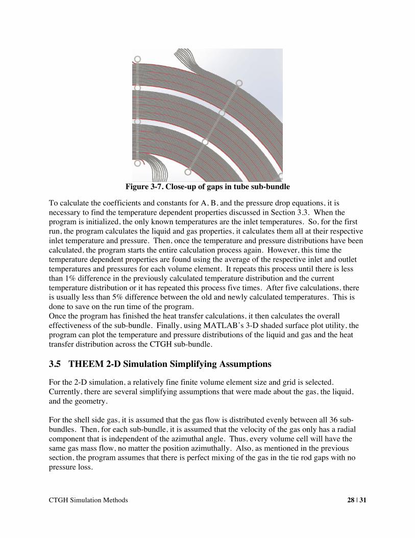
While moving around the bundle loop, the program also calculates the coefficients for most of the gas temperature variables. However, this method assumes that there are no gaps between the tube bundles in the radial direction. As Figure 3-7 shows, there are multiple gaps for the tie rods in each sub-bundle. In order to account for these extra 2 rows of grid spacing, the program adds another 2 rows in the temperature, pressure, and heat transfer matrices. Since there is no tube bundle in these rows, the corresponding spaces will remain blank in the liquid and heat transfer matrices. However, when the gas flows through these gaps, there will be some mixing. For now, the program assumes there is perfect azimuthal mixing of the gas in these gaps. Each gap is bound above and below by the disk spacers between each sub-bundle. The gaps are bound on the sides by the tie bar holders, as shown in Figure 3-7. Since these are stacked so there are no gaps between the holders, the gas will not penetrate them. The program averages the temperatures of the gas entering the gap and assigns it as the outlet temperature for all gas leaving the gap. It is also assumed that there is little to no pressure loss across these gaps. In the future, the program will be modified in order to model gas mixing more realistically in these gaps.


Figure 3-7. Close-up of gaps in tube sub-bundle

To calculate the coefficients and constants for A, B, and the pressure drop equations, it is necessary to find the temperature dependent properties discussed in Section 3.3. When the program is initialized, the only known temperatures are the inlet temperatures. So, for the first run, the program calculates the liquid and gas properties, it calculates them all at their respective inlet temperature and pressure. Then, once the temperature and pressure distributions have been calculated, the program starts the entire calculation process again. However, this time the temperature dependent properties are found using the average of the respective inlet and outlet temperatures and pressures for each volume element. It repeats this process until there is less than 1% difference in the previously calculated temperature distribution and the current temperature distribution or it has repeated this process five times. After five calculations, there is usually less than 5% difference between the old and newly calculated temperatures. This is done to save on the run time of the program. Once the program has finished the heat transfer calculations, it then calculates the overall effectiveness of the sub-bundle. Finally, using MATLAB’s 3-D shaded surface plot utility, the program can plot the temperature and pressure distributions of the liquid and gas and the heat transfer distribution across the CTGH sub-bundle.

3.5 THEEM 2-D Simulation Simplifying Assumptions

For the 2-D simulation, a relatively fine finite volume element size and grid is selected. Currently, there are several simplifying assumptions that were made about the gas, the liquid, and the geometry. For the shell side gas, it is assumed that the gas flow is distributed evenly between all 36 sub-bundles. Then, for each sub-bundle, it is assumed that the velocity of the gas only has a radial component that is independent of the azimuthal angle. Thus, every volume cell will have the same gas mass flow, no matter the position azimuthally. Also, as mentioned in the previous section, the program assumes that there is perfect mixing of the gas in the tie rod gaps with no pressure loss.


For the tube side liquid, the program also assumes that the liquid flow is distributed evenly between all 36 sub-bundles. For each sub-bundle, the liquid flow is assumed to be distributed evenly between all of the manifold pipes and all of the tubes. This implies that the model over-predicts effectiveness, compared to the realistic condition where flow distribution is not perfectly uniform. For the geometry, the model does not calculate the effect of the inlet manifold pipes on the gas flow. It assumes the geometry of the pipes leading into the manifold pipes have the same geometry as the rest of the tube bundle. The model also does not take into account the effect of the gas manifold inlet. It treats the gas duct as perfectly adiabatic so that the inlet temperature of the CTGH is the inlet temperature of each bundle. It also does not take into account any pressure loss that may occur in the duct leading up to the CTGH sub-bundle. Similarly, it assumes that the liquid manifolds are adiabatic and that there is no pressure loss before entering the tubes. Finally, the 2-D simulation does not account for vibrations in the tube bundle. A large flow rate of gas through tube bundles can lead to flow-induced vibrations where the tubes rub together, leading to tube failure. In order to prevent this, anti-vibration spacers will be installed. However, these spacers will block some of the gas flow and reduce the overall gas flow area through the tube bundle. The code does not yet take into account how the gas flow will be affected by these anti-vibration spacers.


4 Conclusion and Future Work

The main focus of future work on the 2-D simulation will be dealing with the simplifying assumptions that are discussed in Section 3.5. An analysis of flow-induced vibrations in the CTGH tube bank will be performed in order to determine the size and placement of the anti-vibration rods in the tube bundles. Once the rods have been incorporated into the design, it will then be possible to include their effect on the air flow calculations. With the construction of a new CTAH mock-up and further research, it will be possible to understand how the air flows through the tie rod gaps. Once this is understood, it should be possible to incorporate this into the model. Then, further experiments will be performed using this mock-up, CTAH Mock-up 2.0, in order to perform more accurate code validation. There may also be some further work on the assumption of purely radial flow. It may be possible to look at CFD programs to get an idea of how to model the flow more realistically between each volume element. It also may be possible to increase the size of the volume elements. This may give more accurate estimations since the simulation uses empirical formulas that account for azimuthal and vertical flow as well as radial flow. Other future work includes the development of a 3-D simulation and a program that builds the optimal CTGH given a point design and desired physical constraints. The 3-D simulation will perform a 2-D simulation on all of the sub-bundles instead of one. It will give a vertical distribution of temperatures and pressures based on the gas and liquid distributions throughout the CTGH as well as the heat transfer that occurs in each sub-bundle. It will also give a more realistic value for the overall heat exchanger effectiveness since it will eliminate many of the assumptions made by the 2-D simulation. The optimization program will use the 0-D model along with an algorithm that changes the CTGH geometry based on desired physical constraints for the heat exchanger. This will make it possible to develop the optimal CTGH for any type of reactor and/or power conversion cycle.


5 References

1. Andreades, Charalampos et al., “Technical Description of the “Mark 1” Pebble-Bed Fluoride-Salt-Cooled High-Temperature Reactor (PB-FHR) Power Plant,” Department of Nuclear Engineering, U.C. Berkeley, Report UCBTH-14-002, September 2014.

2. C. Andreades, R.O. Scarlat, L. Dempsey, and P.F. Peterson, “Reheat Air-Brayton Combined

Cycle (RACC) Power Conversion Design and Performance Under Nominal Ambient Conditions,” ASME Journal of Engineering for Gas Turbines and Power, vol. 136, No. 6, doi:10.1115/1.4026506 (2014).

3. C. Andreades, L. Dempsey, and P.F. Peterson, “Reheat Air-Brayton Combined Cycle

(RACC) Power Conversion Off-Nominal and Transient Performance,” ASME Journal of Engineering for Gas Turbines and Power, vol. 136, No. 7, doi:10.1115/1.4026612 (2014).

4. Incropera, Dewitt, Bergman, Lavine. Introduction to Heat Transfer. 5th ed. Hoboken, NJ:

John Wiley & Sons, 2007.

5. D. F. Williams, L. M. Toth, and K. T. Clarno, “Assessment of candidate molten salt coolants for the advanced high-temperature reactor (AHTR)” ORNL, Oak Ridge, TN, Report ORNL/TM-2006/12, March 2006.

6. Romeo L. Manlapaz & Stuart W. Churchill, “Fully Developed Laminar Convection from a

Helical Coil,” Chemical Engineering Communications, 9:1-6,185-200, DOI: 10.1080/00986448108911023

Simulation Methods for the Characterization of Coiled-Tube ...

Documents

Transcript of Simulation Methods for the Characterization of Coiled-Tube ...