Simulation BIOINFORMATICS - Gerstein Labbioinfo.mbb.yale.edu/mbb452a/simulation/simulation.pdf · 3...

1(c

)M

ark

Ger

stei

n,1

999,

Yal

e,b

ioin

fo.m

bb

.yal

e.ed

u

BIOINFORMATICSSimulation

Mark Gerstein, Yale Universitybioinfo.mbb.yale.edu/mbb452a

2(c

)M

ark

Ger

stei

n,1

999,

Yal

e,b

ioin

fo.m

bb

.yal

e.ed

u

Overview:Electrostatics + Basic Forces

• Electrostatics◊ Polarization◊ Multipoles, dipoles

◊ VDW Forces

◊ Electrostatic Interactions

• Basic Forces◊ Electrical non-bonded interactions

◊ bonded, fundamentally QM but treat as springs

◊ Sum up the energy

• Simple Systems First

3(c

)M

ark

Ger

stei

n,1

999,

Yal

e,b

ioin

fo.m

bb

.yal

e.ed

u

Overview:Methods for the Generation and

Analysis of Macromolecular Simulations

1 Simulation Methods◊ Potential Functions◊ Minimization

◊ Molecular Dynamics

◊ Monte Carlo

◊ Simulated Annealing

2 Types of Analysis◊ liquids: RDFs, Diffusion constants

◊ proteins: RMS, Volumes, Surfaces

• EstablishedTechniques(chemistry, biology,physics)

• Focus on simplesystems first (liquids).Then explain howextended to proteins.

4(c

)M

ark

Ger

stei

n,1

999,

Yal

e,b

ioin

fo.m

bb

.yal

e.ed

u

Electric potential,a quick review

• E = electric field =direction that apositive testcharge wouldmove

• Force/q = E• Potential = W/q =

work per unitcharge = Fx/q =Ex◊ E = - grad φ ; E =

(dφ/dx, dφ/dy, dφ/dz)

Illustration Credit: Purcell

5(c

)M

ark

Ger

stei

n,1

999,

Yal

e,b

ioin

fo.m

bb

.yal

e.ed

u

Maxwell's Equations

• 1st Pair (curl’s)◊ A changing electric field gives

rise to magnetic field that circlesaround it & vice-versa. ElectricCurrent also gives rise tomagnetic field.[no discuss here]

• 2nd Pair (div’s)◊ Relationship of a field to

sources◊ no magnetic monopoles and

magnetostatics: div B = 0[no discuss here]

• All of Electrostatics inGauss's Law!!

cgs (not mks) units above

6(c

)M

ark

Ger

stei

n,1

999,

Yal

e,b

ioin

fo.m

bb

.yal

e.ed

u

MultipoleExpansion

• Routinely done when anatom’s charge distributionis replaced by a pointcharge or a point chargeand a dipole◊ Ignore above dipole here

◊ Harmonic expansion of pot.

• Only applicable far fromthe charge distribution◊ Helix Dipole not meaningful

close-by

• Terms drop off faster withdistance

�++•+=Φ ∑ji

jiij r

xxQ

rr

q

,53 2

1)(

xpx

Replace continuouscharge distribution withpoint moments: charge(monopole) + dipole +quadrupole + octupole + ...

�+++=Φ33

221)(

r

qK

r

qK

r

qKx

7(c

)M

ark

Ger

stei

n,1

999,

Yal

e,b

ioin

fo.m

bb

.yal

e.ed

u

Gauss’ Law: Electrostatics

• div E = 4πρ• Coulomb’s Law

◊ ∫ div E dV = ∫ 4πρ dV◊ ∫ E • dA = ∫ 4πρ dV [Divergence thm.]◊ Assume spherically symmetrical charge distribution

◊ E (4πr2) = 4π Q ==> E = Q/r2

◊ U = - Q/r [assuming a zero at inf.]

• Equations for the Potential Based on the Charge in aRegion plus Boundary Conditions◊ div grad U = 4πρ◊ ∇ 2U = 4πρ [poisson’s equation]◊ ∇ 2U = 0 [Laplace’s equation]

8(c

)M

ark

Ger

stei

n,1

999,

Yal

e,b

ioin

fo.m

bb

.yal

e.ed

u

Dipole Derivation• φ(r, θ) = -q/R1 + q/R2

◊ φ(r, θ) = q(R1- R2)/ R1R2

• If r is very much larger than L◊ Vectors essentially parallel, like

single-slit

◊ R1R2 = r2

◊ R2-R1 = 2L cos θ◊ q(R2-R1) = 2Lqcosθ = p cos θ

= p•r/|r|◊ p = dipole moment vector

= [charge][separation]in direction from neg. to positivecharge

• φ(r, θ) = p cos θ / r2

◊ E = grad φ(r, θ) ~ 1/r3 with acomplex angular dependence

• Monopole is 1/r, whichdominates over dipole (1/r2),dipole dominates quadrupole

L

R1

R2

r

Illustration Credit: Marion & Heald

9(c

)M

ark

Ger

stei

n,1

999,

Yal

e,b

ioin

fo.m

bb

.yal

e.ed

u

Polariz-ation

• Charge shifts to resist field◊ Accomplished perfectly in conductor

-- surface charge, no field inside

◊ Insulators partially accommodate via induced dipoles

• Induced dipole◊ charge/ion movement (slowest)

◊ dipole reorient◊ molecular distort (bond length and angle)

◊ electronic (fastest)

Illustration Credit: Purcell, Marion & Heald

10(c

)M

ark

Ger

stei

n,1

999,

Yal

e,b

ioin

fo.m

bb

.yal

e.ed

u

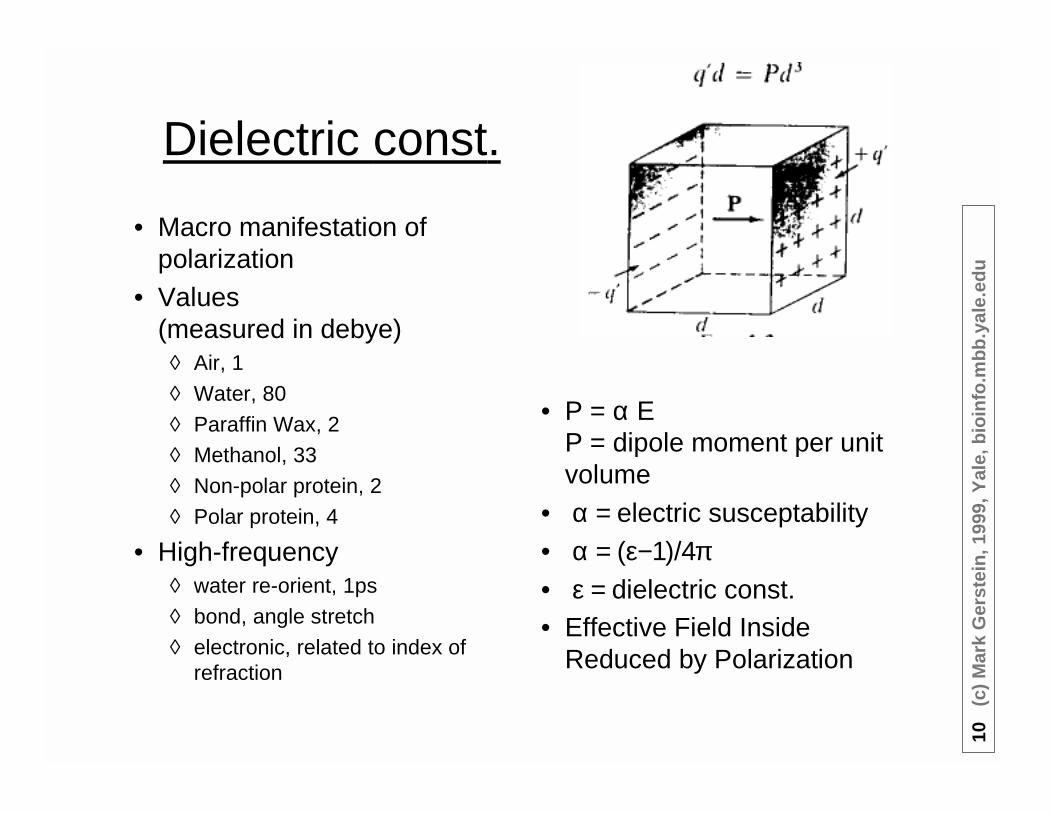
Dielectric const.

• Macro manifestation ofpolarization

• Values(measured in debye)

◊ Air, 1

◊ Water, 80

◊ Paraffin Wax, 2◊ Methanol, 33

◊ Non-polar protein, 2

◊ Polar protein, 4

• High-frequency◊ water re-orient, 1ps

◊ bond, angle stretch

◊ electronic, related to index ofrefraction

• P = α EP = dipole moment per unitvolume

• α = electric susceptability• α = (ε−1)/4π• ε = dielectric const.• Effective Field Inside

Reduced by Polarization

11(c

)M

ark

Ger

stei

n,1

999,

Yal

e,b

ioin

fo.m

bb

.yal

e.ed

u

Polarity vs. PolarizabilityFrom Sharp (1999): “Application of a classical electrostatic view to macromolecular electrostatics involves anumber of useful concepts that describe the physical behavior. It should first be recognized that the

potential at a particular charged atom i includes three physically distinct contributions. The first is thedirect or Coulombic potential of j at i. The second is the potential at i fromthe polarization (from molecule, water and ionic) induced by j. This is oftenreferred to as the screening potential, since it opposes the direct, Coulombicpotential. The third arises from the polarization induced by i itself. This isoften referred to as the reaction or self potential, and if solvent is involved, as thesolvation potential. When using models which apply the concept of a dielectric constant (a measure of

polarizability) to a macromolecule, it is important to distinguish between polarity andpolarizability. Briefly, polarity may be thought of as describing the density of charged and dipolargroups in a particular region. Polarizability, by contrast, refers to the potential for reorganizing charges,orienting dipoles and inducing dipoles. Thus polarizability depends both on the polarity and the freedom ofdipoles to reorganize in response to an applied electric field. When a protein is folding, or undergoing alarge conformational rearrangement, the peptide groups may be quite free to reorient. In the folded proteinthese may become spatially organized so as to stabilize another charge or dipole, creating a region withhigh polarity, but with low polarizability, since there is much less ability to reorient the dipolar groups inresponse to a new charge or dipole without significant disruption of the structure. Thus, while there is stillsome discussion about the value and applicability of a protein dielectric constant, it is generally agreed thatthe interior of a macromolecule is a low polarizable environment compared to solvent. This difference inpolarizability has a significant effect on the potential distribution.”

12(c

)M

ark

Ger

stei

n,1

999,

Yal

e,b

ioin

fo.m

bb

.yal

e.ed

u

VDW Forces:Start byDeriving

Dipole-DipoleEnergy

Simplify. Focus on Formulafor Parallel Dipoles

13(c

)M

ark

Ger

stei

n,1

999,

Yal

e,b

ioin

fo.m

bb

.yal

e.ed

u

AverageDipole-Dipole

InteractionEnergy

• Multiplication ofdipole-dipoleenergy (1/r3) andBoltz. Factor(~dipole-dipoleenergy) gives(1/r6)

14(c

)M

ark

Ger

stei

n,1

999,

Yal

e,b

ioin

fo.m

bb

.yal

e.ed

u

Dipole-induced dipole Energy

• Multipl-ication ofdipole-dipoleenergy(1/r3) andamount ofinduceddipole(1/r3)gives(1/r6)

15(c

)M

ark

Ger

stei

n,1

999,

Yal

e,b

ioin

fo.m

bb

.yal

e.ed

u

VDW Foces:Induced dipole-induced dipole

• Too complex to derive induced-dipole-induced dipoleformula, but it has essential ingredients of dipole-dipole and dipole-induced dipole calculation, giving anattractive 1/r6 dependence.◊ London Forces

• Thus, total dipole cohesive force for molecular systemis the sum of three 1/r6 terms.

• Repulsive forces result from electron overlap.◊ Usually modeled as A/r12 term. Also one can use exp(-Cr).

• VDW forces: V(r) = A/r12 - B/r6 = 4ε((R/r)12 - (R/r)6)◊ ε ~ .2 kcal/mole, R ~ 3.5 A, V ~ .1 kcal/mole [favorable]

16(c

)M

ark

Ger

stei

n,1

999,

Yal

e,b

ioin

fo.m

bb

.yal

e.ed

u

Packing ~ VDW force

• Longer-range isotropic attractive tail provides generalcohesion

• Shorter-ranged repulsion determines detailedgeometry of interaction

• Billiard Ball model, WCA Theory

17(c

)M

ark

Ger

stei

n,1

999,

Yal

e,b

ioin

fo.m

bb

.yal

e.ed

u

Close-packing is Default

• No tight packing whenhighly directionalinteractions(such as H-bonds) needto be satisfied

• Packing spheres (.74),hexagonal

• Water (~.35), “Open”tetrahedral, H-bonds

Illustration Credit: Atkins

18(c

)M

ark

Ger

stei

n,1

999,

Yal

e,b

ioin

fo.m

bb

.yal

e.ed

u

Small PackingChanges

Significant

• Exponentialdependence

• Bounded within arange of 0.5 (.8 and.3)

• Many observationsin standard volumesgives small errorabout the mean(SD/sqrt(N))

atom εεεε(kJ/

mole)

σσσσ(Å)

charge

(electrons)

carbonyl carbon 0.5023 3.7418 0.550

α-carbon (incorporating 1 hydrogen) 0.2034 4.2140 0.100

β-carbon (incorporating 3 hydrogens) 0.7581 3.8576 0.000

amide nitrogen 0.9979 2.8509 -0.350

amide hydrogen 0.2085 1.4254 0.250

carbonyl oxygen 0.6660 2.8509 -0.550

water oxygen in interactions with the helix 0.6660 2.8509 -0.834

water hydrogen in interactions with the helix 0.2085 1.4254 0.417

water O in interactions with other waters 0.6367 3.1506 -0.834

water H in interactions with other waters 0.0000 0.0000 0.417

19(c

)M

ark

Ger

stei

n,1

999,

Yal

e,b

ioin

fo.m

bb

.yal

e.ed

u

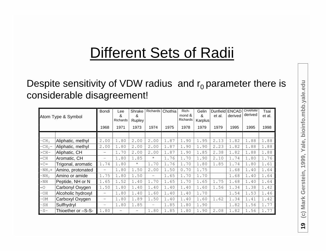
Different Sets of Radii

Atom Type & SymbolBondi Lee

&Richards

Shrake&

Rupley

Richards Chothia Rich-mond &Richards

Gelin&

Karplus

Dunfieldet al.

ENCADderived

CHARMM

derivedTsaiet al.

1968 1971 1973 1974 1975 1978 1979 1979 1995 1995 1998

-CH3 Aliphatic, methyl 2.00 1.80 2.00 2.00 1.87 1.90 1.95 2.13 1.82 1.88 1.88-CH2- Aliphatic, methyl 2.00 1.80 2.00 2.00 1.87 1.90 1.90 2.23 1.82 1.88 1.88>CH- Aliphatic, CH - 1.70 2.00 2.00 1.87 1.90 1.85 2.38 1.82 1.88 1.88=CH Aromatic, CH - 1.80 1.85 * 1.76 1.70 1.90 2.10 1.74 1.80 1.76>C= Trigonal, aromatic 1.74 1.80 * 1.70 1.76 1.70 1.80 1.85 1.74 1.80 1.61-NH3+ Amino, protonated - 1.80 1.50 2.00 1.50 0.70 1.75 1.68 1.40 1.64-NH2 Amino or amide 1.75 1.80 1.50 - 1.65 1.70 1.70 1.68 1.40 1.64>NH Peptide, NH or N 1.65 1.52 1.40 1.70 1.65 1.70 1.65 1.75 1.68 1.40 1.64=O Carbonyl Oxygen 1.50 1.80 1.40 1.40 1.40 1.40 1.60 1.56 1.34 1.38 1.42-OH Alcoholic hydroxyl - 1.80 1.40 1.60 1.40 1.40 1.70 1.54 1.53 1.46-OM Carboxyl Oxygen - 1.80 1.89 1.50 1.40 1.40 1.60 1.62 1.34 1.41 1.42-SH Sulfhydryl - 1.80 1.85 - 1.85 1.80 1.90 1.82 1.56 1.77-S- Thioether or –S-S- 1.80 - - 1.80 1.85 1.80 1.90 2.08 1.82 1.56 1.77

Despite sensitivity of VDW radius and r0 parameter there isconsiderable disagreement!

20(c

)M

ark

Ger

stei

n,1

999,

Yal

e,b

ioin

fo.m

bb

.yal

e.ed

u

MolecularMechanics:

Simpleelectrostatics

• U = kqQ/r• Molecular mechanics

uses partial unpaired charges with monopole◊ usually no dipole

◊ e.g. water has apx. -.8 on O and +.4 on Hs

◊ However, normally only usemonopoles for unpaired charges (on charged atoms, asp O)

• Longest-range force◊ Truncation? Smoothing

atom εεεε(kJ/

mole)

σσσσ(Å)

charge

(electrons)

carbonyl carbon 0.5023 3.7418 0.550

α-carbon (incorporating 1 hydrogen) 0.2034 4.2140 0.100

β-carbon (incorporating 3 hydrogens) 0.7581 3.8576 0.000

amide nitrogen 0.9979 2.8509 -0.350

amide hydrogen 0.2085 1.4254 0.250

carbonyl oxygen 0.6660 2.8509 -0.550

water oxygen in interactions with the helix 0.6660 2.8509 -0.834

water hydrogen in interactions with the helix 0.2085 1.4254 0.417

water O in interactions with other waters 0.6367 3.1506 -0.834

water H in interactions with other waters 0.0000 0.0000 0.417

21(c

)M

ark

Ger

stei

n,1

999,

Yal

e,b

ioin

fo.m

bb

.yal

e.ed

u

H-bonds subsumed byelectrostatic interactions

• Naturally arise from partial charges◊ normally arise from partial charge

• Linear geometry• Were explicit springs in older models

Illustration Credit: Taylor & Kennard (1984)

22(c

)M

ark

Ger

stei

n,1

999,

Yal

e,b

ioin

fo.m

bb

.yal

e.ed

u

BondLengthSprings

• F= -kx -> E = kx2/2• Freq from IR spectroscopy

◊ -> w= sqrt(k/m), m = mass => spring const. k◊ k ~ 500 kcal/mole*A2 (stiff!),

w corresponds to a period of 10 fs

• Bond length have 2-centers

x

F

C C

x0=1.5A

23(c

)M

ark

Ger

stei

n,1

999,

Yal

e,b

ioin

fo.m

bb

.yal

e.ed

u

Bond angle, More Springs

• torque = τ = κθ -> E = κθ2/2• 3-centers

N C

C

24(c

)M

ark

Ger

stei

n,1

999,

Yal

e,b

ioin

fo.m

bb

.yal

e.ed

u

Torsion angle• 4-centers• U(A)=K(1-cos(nA+d))

◊ cos x = 1 + x2/2 + ... ,so minima are quitespring like, but one canhoop between barriers

• K ~ 2 kcal/mole

Torsion Angle A -->

60 180 -60

U

25(c

)M

ark

Ger

stei

n,1

999,

Yal

e,b

ioin

fo.m

bb

.yal

e.ed

u

PotentialFunctions

• Putting it alltogether

• Springs +ElectricalForces

26(c

)M

ark

Ger

stei

n,1

999,

Yal

e,b

ioin

fo.m

bb

.yal

e.ed

u

Sum up toget totalenergy

• Each atom is apoint mass(m and x)

• Sometimes specialpseudo-forces:torsions andimproper torsions,H-bonds, symmetry.

27(c

)M

ark

Ger

stei

n,1

999,

Yal

e,b

ioin

fo.m

bb

.yal

e.ed

u

EnergyScale of

Interactions

Illustration Credit: M Levitt

28(c

)M

ark

Ger

stei

n,1

999,

Yal

e,b

ioin

fo.m

bb

.yal

e.ed

u

Elaboration on the Basic Protein Model• Geometry

◊ Start with X, Y, Z’s (coordinates)

◊ Derive Distance, Surface Area,Volume, Axes, Angle, &c

• Energetics◊ Add Q’s and k’s (Charges for

electrical forces, Force Constants forsprings)

◊ Derive Potential Function U(x)

• Dynamics◊ Add m’s and t (mass and time)

◊ Derive Dynamics(v=dx/dt, F = m dv/dt)

29(c

)M

ark

Ger

stei

n,1

999,

Yal

e,b

ioin

fo.m

bb

.yal

e.ed

u

Goal:Model

Proteinsand

NucleicAcids

as RealPhysical

Molecules

30(c

)M

ark

Ger

stei

n,1

999,

Yal

e,b

ioin

fo.m

bb

.yal

e.ed

u

Ways to Move Proteinon its Energy Surface

Minimization Normal Mode Analysis (later?)

Molecular Dynamics (MD) Monte Carlo (MC)

random

Illustration Credit: M Levitt

31(c

)M

ark

Ger

stei

n,1

999,

Yal

e,b

ioin

fo.m

bb

.yal

e.ed

u

Steepest Descent Minimization

• Particles on an “energylandscape.” Search forminimum energyconfiguration

◊ Get stuck in local minima

• Steepest descentminimization

◊ Follow gradient of energy straightdownhill

◊ i.e. Follow the force:step ~ F = -∇∇∇∇ Usox(t) = x(t-1) + a F/|F|

32(c

)M

ark

Ger

stei

n,1

999,

Yal

e,b

ioin

fo.m

bb

.yal

e.ed

u

Multi-dimensionalMinimization

• In many dimensions, minimizealong lines one at a time

• Ex: U = x2+5y2 , F = (2x,10y)

Illustration Credit: Biosym, discover manual

33(c

)M

ark

Ger

stei

n,1

999,

Yal

e,b

ioin

fo.m

bb

.yal

e.ed

u

Other Minimization Methods

• Problem is that get stuck in local minima• Steepest descent, least clever but robust,

slow at end• Newton-Raphson faster but 2nd deriv. can

be fooled by harmonic assumption• Recipe: steepest descent 1st, then

Newton-raph. (or conj. grad.)

• Simplex, grid search◊ no derivatives

• Conjugate gradientstep ~ F(t) - bF(t-1)

◊ partial 2nd derivative

• Newton-Raphson◊ using 2nd derivative, find

minimum assuming it isparabolic

◊ V = ax2 + bx + c

◊ V' =2ax + b & V" =2a

◊ V' =0 -> x* = -b/2a

34(c

)M

ark

Ger

stei

n,1

999,

Yal

e,b

ioin

fo.m

bb

.yal

e.ed

u

Adiabaticmapping

• Interpolate thenminimize◊ Gives apx. energy

(H) landscapethrough a barrier

◊ can sort of estimatetransition raterate = (kT/h) exp (-dG/kT)

◊ Used for ring flips,hinge motions

35(c

)M

ark

Ger

stei

n,1

999,

Yal

e,b

ioin

fo.m

bb

.yal

e.ed

u

MolecularDynamics

• Give each atoms a velocity.◊ If no forces, new position of atom

(at t + dt) would be determinedonly by velocityx(t+dt) = x(t) + v dt

• Forces change the velocity,complicating thingsimmensely◊ F = dp/dt = m dv/dt

36(c

)M

ark

Ger

stei

n,1

999,

Yal

e,b

ioin

fo.m

bb

.yal

e.ed

u

Molecular Dynamics (cont)

• On computer make very smallsteps so force is nearly constantand velocity change can becalculated (uniform a)

[Avg. v over ∆t] = (v + ∆v/2)

• Trivial to update positions:

• Step must be very small◊ ∆t ~ 1fs

(atom moves 1/500 of itsdiameter)

◊ This is why you need fastcomputers

• Actual integrationschemes slightly morecomplicated

◊ Verlet (explicit half-step)

◊ Beeman, Gear(higher order terms thanacceleration)

∆v =Fm

∆t

x(t + ∆t ) = x(t ) + (v + ∆v2

)∆t

= x(t ) + v∆t +F

2m∆t 2

37(c

)M

ark

Ger

stei

n,1

999,

Yal

e,b

ioin

fo.m

bb

.yal

e.ed

u

Phase Space Walk• Trajectories of all the particles traverses space of all possible

configuration and velocity states (phase space)

• Ergodic Assumption:Eventually, trajectory visits every state in phase space

• Boltzmann weighting:Throughout, trajectory samples states fairly in terms of system’senergy levels

◊ More time in low-U than high-U states◊ Probability of being in a

state ~ exp(-U/kT)

• Consequently, statistics (average properties) over trajectory arethermodynamically correct

38(c

)M

ark

Ger

stei

n,1

999,

Yal

e,b

ioin

fo.m

bb

.yal

e.ed

u

ExamplePhaseSpaceWalk

X = 3X A + 3XB + 2XA +1XD

U = 6UAB + 2U A +1U D

39(c

)M

ark

Ger

stei

n,1

999,

Yal

e,b

ioin

fo.m

bb

.yal

e.ed

u

Monte Carlo

• Other ways than MD tosample states fairly andcompute correctlyweighted averages?Yes, using Monte Carlocalculations.

• Basic Idea:Move through statesrandomly, accepting orrejecting them so onegets a correct“Boltzmann weighting”

• Formalism:◊ System described by a probability

distribution ρ(n) for it to be in each state n

◊ Random (“Markov”) process πoperateson the system and changes distributionamongst states to πρ(n)

◊ At equilbrium original distribution and newdistribution have to be same asBoltzmann distribution

πρ(n ) = ρ (n ) =1Z

exp−U (n )

kT

40(c

)M

ark

Ger

stei

n,1

999,

Yal

e,b

ioin

fo.m

bb

.yal

e.ed

u

Monte Carlo(cont)

• Metropolis Rule(for specifying π )

1 Make a random move to aparticle and calculate the energychange dU

2 dU < 0 −> accept the move3 Otherwise, compute a random

number R between 0 and 1:R < ~ exp(-U/kT) −>

accept the moveotherwise −>

reject the move

• “Fun” example of MC Integration◊ Particle in empty

box of side 2r(energy of all states same)

◊ π= 6 x [Fraction of times particles iswithin r of center]

41(c

)M

ark

Ger

stei

n,1

999,

Yal

e,b

ioin

fo.m

bb

.yal

e.ed

u

MC vs/+ MD

• MD usually used for proteins. Difficult to make moveswith complicated chain.

• MC often used for liquids. Can be made into a veryefficient sampler.

• Hybrid approaches (Brownian dynamics)• Simulated Annealing. Heat simulation up to high T

then gradually cool and minimize to find globalminimum.

42(c

)M

ark

Ger

stei

n,1

999,

Yal

e,b

ioin

fo.m

bb

.yal

e.ed

u

MovingMolecules

Rigidly

• Rigid-body Rotation of all i atoms◊ For each atom atom i do

xi(t+1) = R(φ,θ,ψ) xi(t)◊ Effectively do a rotation around each axis (x, y, z)

by angles φ,θ,ψ (see below)◊ Many conventions for doing this

• BELOW IS ONLY FOR MOTIVATION• Consult Allen & Tildesley (1987) or Goldstein

for the formulation of the rotation matrixusing the usual conventions

◊ How does one do a random rotation? Trickierthan it seems

−=

y

x

y

x

θθθθ

cossin

sincos

'

'

−

−

−=

z

y

x

z

y

x

��

axisxaroundbyrotateFirst,axisyaroundbyrotateSecond,axiszaroundbyrotateFinally,

cossin0

sincos0

001

cos0sin

010

sin0cos

100

0cossin

0sincos

'

'

'

ψφθ

ψψψψ

φφ

φφθθθθ

• Xi(t+1) = (xi(t),yi(t),zi(t))= coordinates of ith atomin the molecule attimestep t

• Rigid-body Translation ofall i atoms

◊ For each atom atom i doxi(t+1) = xi(t) + v

43 (c) Mark Gerstein, 1999, Yale, bioinfo.mbb.yale.edu

TypicalS

ystems:W

aterv.A

rgon


Typical

System

s:D

NA

+W

ater


TypicalS

ystems:P

rotein+

Water

46(c

)M

ark

Ger

stei

n,1

999,

Yal

e,b

ioin

fo.m

bb

.yal

e.ed

u

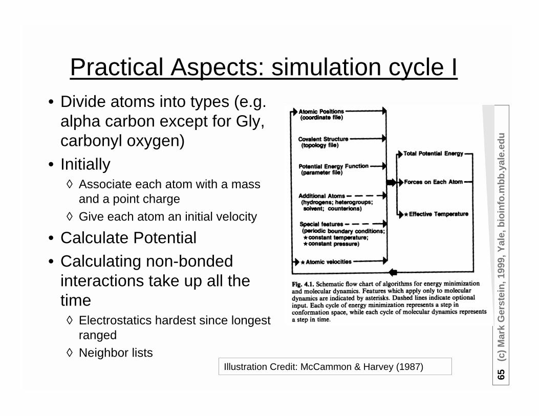
Practical Aspects: simulation cycle I• Divide atoms into types (e.g.

alpha carbon except for Gly,carbonyl oxygen)

• Initially◊ Associate each atom with a mass

and a point charge

◊ Give each atom an initial velocity

• Calculate Potential• Calculating non-bonded

interactions take up all thetime◊ Electrostatics hardest since longest

ranged◊ Neighbor lists

Illustration Credit: McCammon & Harvey (1987)

47(c

)M

ark

Ger

stei

n,1

999,

Yal

e,b

ioin

fo.m

bb

.yal

e.ed

u

Practical Aspects: simulation cycle II• Update Positions with MD

equations, then recalculatepotential and continue

• Momentum conservation• Energy Conserved in NVE

ensemble• Hydrophobic interaction

naturally arises from waterbehavior


48(c

)M

ark

Ger

stei

n,1

999,

Yal

e,b

ioin

fo.m

bb

.yal

e.ed

u

SampleProtein

Parameters(toph19.pro)

REMARKS TOPH19.PRO ( protein topology )REMARKS ===============================REMARKS Charges and atom order modified for neutral GROUPs.REMARKS Histidine charges set to Del Bene and Cohen sto-3g calculations.REMARKS Amide charges set to match the experimental dipole moment.REMARKS Default for HIStidines is the doubly protonated state

set echo=false end!! for use with PARAM19 parameters ( no special hydrogen bonding potential )!! donor and acceptor terms just for analysis

AUTOGENERATE ANGLES=TRUE END{*===========================*}

{* protein default masses *}MASS H 1.00800! hydrogen which can h-bond to neutral atomMASS HC 1.00800! ="= ="= ="= to charged atomMASS HA 1.00800! aliphatic hydrogenMASS CT 12.01100! aliphatic carbonMASS C 12.01100! carbonyl carbonMASS CH1E 13.01900! extended atom carbon with one hydrogenMASS CH2E 14.02700! ="= ="= ="= two hydrogensMASS CH3E 15.03500! ="= ="= ="= three hydrogensMASS CR1E 13.01900! ="= ="= in an aromatic ring with one HMASS N 14.00670! peptide nitrogen with no hydrogens attachedMASS NR 14.00670! nitrogen in an aromatic ring with no hydrogensMASS NP 14.00670! pyrole nitrogenMASS NH1 14.00670! peptide nitrogen bound to one hydrogenMASS NH2 14.00670! ="= ="= ="= two hydrogensMASS NH3 14.00670! nitrogen bound to three hydrogensMASS NC2 14.00670! charged guandinium nitrogen bound to two hydrogensMASS O 15.99940! carbonyl oxygenMASS OC 15.99940! carboxy oxygenMASS OH1 15.99940! hydroxy oxygenMASS S 32.06000! sulphurMASS SH1E 33.06800! extended atom sulfur with one hydrogen

!some empirical rules for the following topologies:!

49(c

)M

ark

Ger

stei

n,1

999,

Yal

e,b

ioin

fo.m

bb

.yal

e.ed

u

SampleProtein

Parameters(toph19.pro)

. RESIdue ALAGROUpATOM N TYPE=NH1 CHARge=-0.35 ENDATOM H TYPE=H CHARge= 0.25 ENDATOM CA TYPE=CH1E CHARge= 0.10 END

GROUpATOM CB TYPE=CH3E CHARge= 0.00 END

GROUpATOM C TYPE=C CHARge= 0.55 END !#ATOM O TYPE=O CHARge=-0.55 END !#

BOND N CABOND CA CBOND C OBOND N HBOND CA CB

IMPRoper CA N C CB !tetrahedral CA

DONOr H NACCEptor O C

IC N C *CA CB 0.0000 0.00 120.00 0.00 0.0000

END {ALA}

!------------------------------------------------------------------

RESIdue ARGGROUpATOM N TYPE=NH1 CHARge=-0.35 ENDATOM H TYPE=H CHARge= 0.25 ENDATOM CA TYPE=CH1E CHARge= 0.10 END

GROUpATOM CB TYPE=CH2E CHARge= 0.00 ENDATOM CG TYPE=CH2E CHARge= 0.00 END

GROUpATOM CD TYPE=CH2E CHARge= 0.10 END !#ATOM NE TYPE=NH1 CHARge=-0.40 END !#

50(c

)M

ark

Ger

stei

n,1

999,

Yal

e,b

ioin

fo.m

bb

.yal

e.ed

u

SampleProtein

Parameters(param19.pro)

remark - parameter file PARAM19 -

bond C C 450.0 1.38! B. R. GELIN THESIS AMIDE AND DIPEPTIDESbond C CH1E 405.0 1.52! EXCEPT WHERE NOTED. CH1E,CH2E,CH3E, AND CTbond C CH2E 405.0 1.52! ALL TREATED THE SAME. UREY BRADLEY TERMS ADDEDbond C CH3E 405.0 1.52bond C CR1E 450.0 1.38bond C CT 405.0 1.53bond C N 471.0 1.33bond C NC2 400.0 1.33! BOND LENGTH FROM PARMFIX9 FORCE K APROXIMATEbond C NH1 471.0 1.33bond C NH2 471.0 1.33bond C NP 471.0 1.33bond C NR 471.0 1.33bond C O 580.0 1.23bond C OC 580.0 1.23! FORCE DECREASE AND LENGTH INCREASE FROM C Obond C OH1 450.0 1.38! FROM PARMFIX9 (NO VALUE IN GELIN THESIS)bond C OS 292.0 1.43! FROM DEP NORMAL MODE FITbond CH1E CH1E 225.0 1.53bond CH1E CH2E 225.0 1.52bond CH1E CH3E 225.0 1.52bond CH1E N 422.0 1.45bond CH1E NH1 422.0 1.45bond CH1E NH2 422.0 1.45bond CH1E NH3 422.0 1.45bond CH1E OH1 400.0 1.42! FROM PARMFIX9 (NO VALUE IN GELIN THESIS)bond CH2E CH2E 225.0 1.52bond CH2E CH3E 225.0 1.54bond CH2E CR1E 250.0 1.45! FROM WARSHEL AND KARPLUS 1972 JACS 96:5612bond CH2E N 422.0 1.45bond CH2E NH1 422.0 1.45bond CH2E NH2 422.0 1.45bond CH2E NH3 422.0 1.45bond CH2E OH1 400.0 1.42bond CH2E S 450.0 1.81! FROM PARMFIX9bond CH2E SH1E 450.0 1.81b d H3E NH1 422 0 1 49

51(c

)M

ark

Ger

stei

n,1

999,

Yal

e,b

ioin

fo.m

bb

.yal

e.ed

u

SampleProtein


angle C C C 70.0 106.5! FROM B. R. GELIN THESIS WITH HARMONICangle C C CH2E 65.0 126.5! PART OF F TERMS INCORPORATED. ATOMSangle C C CH3E 65.0 126.5! WITH EXTENDED H COMPENSATED FOR LACKangle C C CR1E 70.0 122.5! OF H ANGLES.angle C C CT 70.0 126.5angle C C HA 40.0 120.0! AMIDE PARAMETERS FIT BY LEAST SQUARESangle C C NH1 65.0 109.0! TO N-METHYL ACETAMIDE VIBRATIONS.angle C C NP 65.0 112.5! MINIMIZATION OF N-METHYL ACETAMIDE.angle C C NR 65.0 112.5angle C C OH1 65.0 119.0angle C C O 65.0 119.0 ! FOR NETROPSINangle CH1E C N 20.0 117.5angle CH1E C NH1 20.0 117.5angle CH1E C O 85.0 121.5angle CH1E C OC 85.0 117.5angle CH1E C OH1 85.0 120.0angle CH2E C CR1E 70.0 121.5angle CH2E C N 20.0 117.5angle CH2E C NH1 20.0 117.5angle CH2E C NH2 20.0 117.5angle CH2E C NC2 20.0 117.5 ! FOR NETROPSINangle CH2E C NR 60.0 116.0angle CH2E C O 85.0 121.6angle CH2E C OC 85.0 118.5angle CH2E C OH1 85.0 120.0angle CH3E C N 20.0 117.5angle CH3E C NH1 20.0 117.5angle CH3E C O 85.0 121.5angle CR1E C CR1E 65.0 120.5angle CR1E C NH1 65.0 110.5! USED ONLY IN HIS, NOT IT TRPangle CR1E C NP 65.0 122.5angle CR1E C NR 65.0 122.5angle CR1E C OH1 65.0 119.0angle CT C N 20.0 117.5angle CT C NH1 20.0 117.5angle CT C NH2 20.0 117.5angle CT C O 85.0 121.5angle CT C OC 85.0 118.5angle CT C OH1 85.0 120.0angle HA C NH1 40.0 120.0angle HA NH2 40 0 120 0

52(c

)M

ark

Ger

stei

n,1

999,

Yal

e,b

ioin

fo.m

bb

.yal

e.ed

u

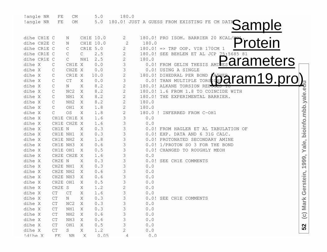
SampleProtein


!angle NR FE CM 5.0 180.0!angle NR FE OM 5.0 180.0! JUST A GUESS FROM EXISTING FE CM DATA

dihe CH1E C N CH1E 10.0 2 180.0! PRO ISOM. BARRIER 20 KCAL/MOL.dihe CH2E C N CH1E 10.0 2 180.0dihe CR1E C C CR1E 5.0 2 180.0! => TRP OOP. VIB 170CM 1dihe CR1E C C C 2.5 2 180.0! SEE BEHLEN ET AL JCP 75:5685 81dihe CR1E C C NH1 2.5 2 180.0dihe X C CH1E X 0.0 3 0.0! FROM GELIN THESIS AMIDESdihe X C CH2E X 0.0 3 0.0! USING A SINGLEdihe X C CR1E X 10.0 2 180.0! DIHEDRAL PER BOND RATHERdihe X C CT X 0.0 3 0.0! THAN MULTIPLE TORSIONS.dihe X C N X 8.2 2 180.0! ALKANE TORSION REDUCED TOdihe X C NC2 X 8.2 2 180.0! 1.6 FROM 1.8 TO COINCIDE WITHdihe X C NH1 X 8.2 2 180.0! THE EXPERIMENTAL BARRIER.dihe X C NH2 X 8.2 2 180.0dihe X C OH1 X 1.8 2 180.0dihe X C OS X 1.8 2 180.0 ! INFERRED FROM C-OH1dihe X CH1E CH1E X 1.6 3 0.0dihe X CH1E CH2E X 1.6 3 0.0dihe X CH1E N X 0.3 3 0.0! FROM HAGLER ET AL TABULATION OFdihe X CH1E NH1 X 0.3 3 0.0! EXP. DATA AND 6 31G CALC.dihe X CH1E NH2 X 1.8 3 0.0! PROTONATED SECONDARY AMINEdihe X CH1E NH3 X 0.6 3 0.0! 1/PROTON SO 3 FOR THE BONDdihe X CH1E OH1 X 0.5 3 0.0! CHANGED TO ROUGHLY MEOHdihe X CH2E CH2E X 1.6 3 0.0dihe X CH2E N X 0.3 3 0.0! SEE CH1E COMMENTSdihe X CH2E NH1 X 0.3 3 0.0dihe X CH2E NH2 X 0.6 3 0.0dihe X CH2E NH3 X 0.6 3 0.0dihe X CH2E OH1 X 0.5 3 0.0dihe X CH2E S X 1.2 2 0.0dihe X CT CT X 1.6 3 0.0dihe X CT N X 0.3 3 0.0! SEE CH1E COMMENTSdihe X CT NC2 X 0.3 3 0.0dihe X CT NH1 X 0.3 3 0.0dihe X CT NH2 X 0.6 3 0.0dihe X CT NH3 X 0.6 3 0.0dihe X CT OH1 X 0.5 3 0.0dihe X CT S X 1.2 2 0.0!dihe X FE NR X 0.05 4 0.0

53(c

)M

ark

Ger

stei

n,1

999,

Yal

e,b

ioin

fo.m

bb

.yal

e.ed

u

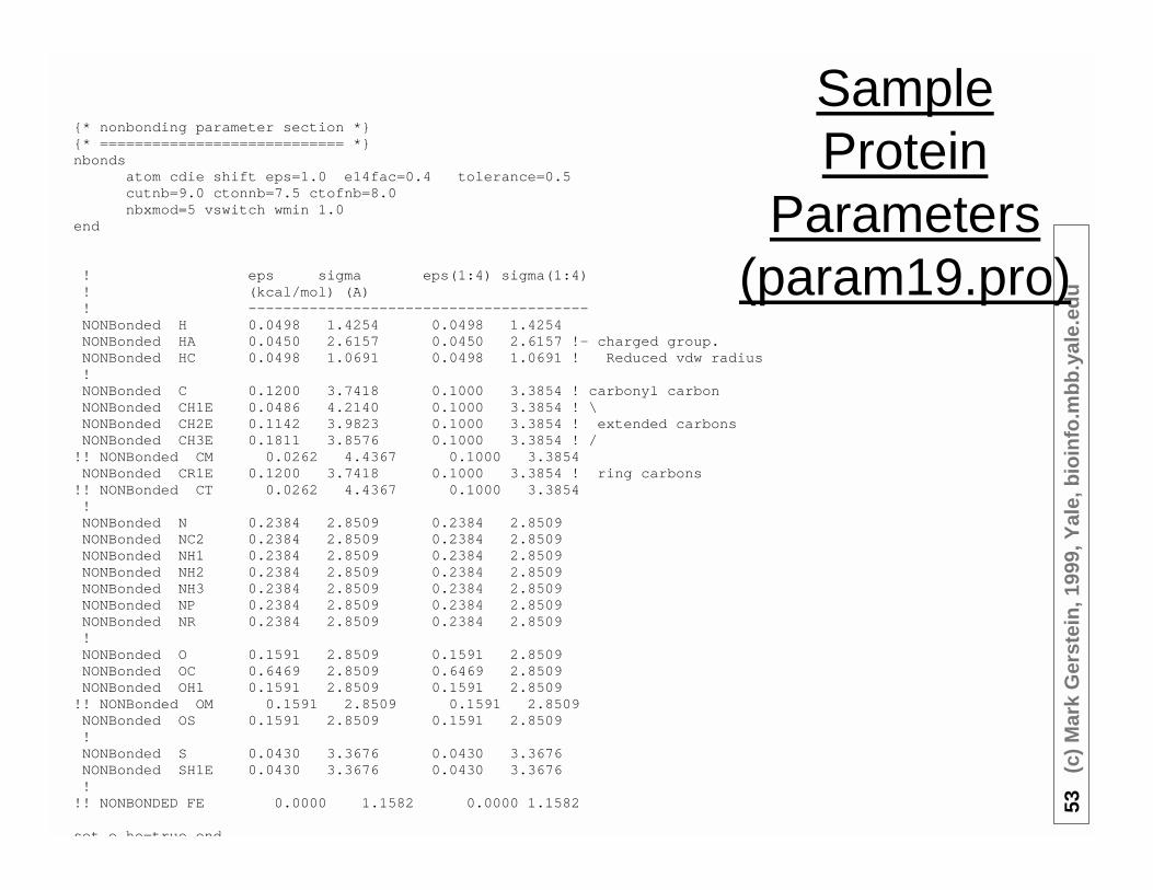
SampleProtein


{* nonbonding parameter section *}{* ============================ *}nbonds

atom cdie shift eps=1.0 e14fac=0.4 tolerance=0.5cutnb=9.0 ctonnb=7.5 ctofnb=8.0nbxmod=5 vswitch wmin 1.0

end

! eps sigma eps(1:4) sigma(1:4)! (kcal/mol) (A)! ---------------------------------------NONBonded H 0.0498 1.4254 0.0498 1.4254NONBonded HA 0.0450 2.6157 0.0450 2.6157 !- charged group.NONBonded HC 0.0498 1.0691 0.0498 1.0691 ! Reduced vdw radius!NONBonded C 0.1200 3.7418 0.1000 3.3854 ! carbonyl carbonNONBonded CH1E 0.0486 4.2140 0.1000 3.3854 ! \NONBonded CH2E 0.1142 3.9823 0.1000 3.3854 ! extended carbonsNONBonded CH3E 0.1811 3.8576 0.1000 3.3854 ! /

!! NONBonded CM 0.0262 4.4367 0.1000 3.3854NONBonded CR1E 0.1200 3.7418 0.1000 3.3854 ! ring carbons

!! NONBonded CT 0.0262 4.4367 0.1000 3.3854!NONBonded N 0.2384 2.8509 0.2384 2.8509NONBonded NC2 0.2384 2.8509 0.2384 2.8509NONBonded NH1 0.2384 2.8509 0.2384 2.8509NONBonded NH2 0.2384 2.8509 0.2384 2.8509NONBonded NH3 0.2384 2.8509 0.2384 2.8509NONBonded NP 0.2384 2.8509 0.2384 2.8509NONBonded NR 0.2384 2.8509 0.2384 2.8509!NONBonded O 0.1591 2.8509 0.1591 2.8509NONBonded OC 0.6469 2.8509 0.6469 2.8509NONBonded OH1 0.1591 2.8509 0.1591 2.8509

!! NONBonded OM 0.1591 2.8509 0.1591 2.8509NONBonded OS 0.1591 2.8509 0.1591 2.8509!NONBonded S 0.0430 3.3676 0.0430 3.3676NONBonded SH1E 0.0430 3.3676 0.0430 3.3676!

!! NONBONDED FE 0.0000 1.1582 0.0000 1.1582

set e ho=true end

54(c

)M

ark

Ger

stei

n,1

999,

Yal

e,b

ioin

fo.m

bb

.yal

e.ed

u

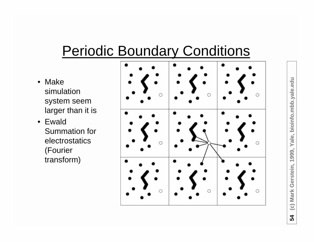
Periodic Boundary Conditions

• Makesimulationsystem seemlarger than it is

• EwaldSummation forelectrostatics(Fouriertransform)

55(c

)M

ark

Ger

stei

n,1

999,

Yal

e,b

ioin

fo.m

bb

.yal

e.ed

u

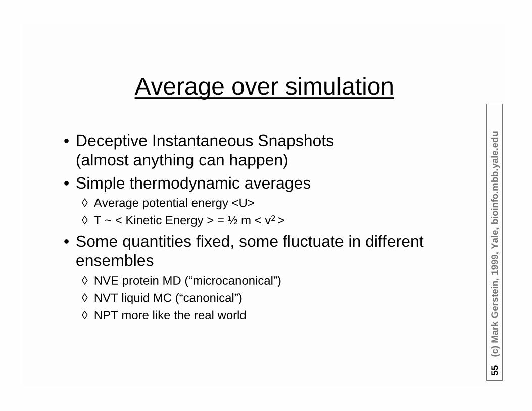
Average over simulation

• Deceptive Instantaneous Snapshots(almost anything can happen)

• Simple thermodynamic averages◊ Average potential energy <U>

◊ T ~ < Kinetic Energy > = ½ m < v2 >

• Some quantities fixed, some fluctuate in differentensembles◊ NVE protein MD (“microcanonical”)◊ NVT liquid MC (“canonical”)

◊ NPT more like the real world

56(c

)M

ark

Ger

stei

n,1

999,

Yal

e,b

ioin

fo.m

bb

.yal

e.ed

uTimescales

Motion length time

(Å) (fs)

bond vibration 0.1 10

water hindered rotation 0.5 1000

surface sidechain rotation 5 105

water diffusive motion 4 105

buried sidechain libration 0.5 105

hinge bending of chain 3 106

buried sidechain rotation 5 1013

allosteric transition 3 1013

local denaturation 7 1014

(FromMcCammon &Harvey,Eisenberg &Kauzmann)

57(c

)M

ark

Ger

stei

n,1

999,

Yal

e,b

ioin

fo.m

bb

.yal

e.ed

u

D & RMS

• Diffusion constant◊ Measures average rate of

increase in variance of position ofthe particles

◊ Suitable for liquids, not really forproteins

D =∆r 2

6∆t

RMS (t ) =di (t )

i =1

N∑N

di (t ) = R(xi (t ) − T) − xi (0)

• RMS more suitable toproteins

◊ di = Difference in position ofprotein atom at t from the initialposition, after structures havebeen optimally rotated translatedto minimize RMS(t)

◊ Solution of optimal rotation hasbeen solved a number of ways(Kabsch, SVD)

58(c

)M

ark

Ger

stei

n,1

999,

Yal

e,b

ioin

fo.m

bb

.yal

e.ed

u

NumberDensity

= Number of atoms per unit volume averaged over simulation divided bythe number you expect to have in the same volume of an ideal “gas”

Spatially average over all directions gives

1D RDF =

[ Avg. Num. Neighbors at r ][Expected Num. Neighbors at r ]

“at r” means contained in a thin shell of thickness dr and radius r.

59(c

)M

ark

Ger

stei

n,1

999,

Yal

e,b

ioin

fo.m

bb

.yal

e.ed

u

Number Density (cont)• Advantages: Intuitive,

Relates to scattering expts• D/A: Not applicable to real

proteins◊ 1D RDF not structural

◊ 2D proj. only useful with "toy"systems

• Number densitiesmeasure spatialcorrelations, not packing

◊ Low value does not implycavities

◊ Complicated by asymmetricmolecules

◊ How things pack and fit isproperty of instantaneousstructure - not average

60(c

)M

ark

Ger

stei

n,1

999,

Yal

e,b

ioin

fo.m

bb

.yal

e.ed

u

Major Protein Simulation Packages

• AMBER◊ http://www.amber.ucsf.edu/amber/amber.html

◊ http://www.amber.ucsf.edu/amber/tutorial/index.html

• CHARMM/XPLOR◊ http://yuri.harvard.edu/charmm/charmm.html

◊ http://atb.csb.yale.edu/xplor◊ http://uracil.cmc.uab.edu/Tutorials/default.html

• ENCAD• GROMOS

◊ http://rugmd0.chem.rug.nl/md.html

◊ “Advanced Crash Course on Electrostatics in Simulations” (!)(http://rugmd0.chem.rug.nl/~berends/course.html)

61(c

)M

ark

Ger

stei

n,1

999,

Yal

e,b

ioin

fo.m

bb

.yal

e.ed

u

Molecular Biophysics & Biochemistry400a/700a (Advanced Biochemistry)

Computational Aspects of:Simulation (Part II),

Electrostatics (Part II),Water and Hydrophobicity

Mark Gerstein

Classes on 11/12/98 & 10/17/98Yale University

62(c

)M

ark

Ger

stei

n,1

999,

Yal

e,b

ioin

fo.m

bb

.yal

e.ed

u

The Handouts

• Notes

◊ Coming on Tuesday!!!◊ Perhaps available on-line at http://bioinfo.mbb.yale.edu/course

• Presentation Paper◊ Duan, Y. & Kollman, P. A. (1998). Pathways to a protein folding intermediate

observed in a 1-microsecond simulation in aqueous solution Science 282,740-4.

• http://bioinfo.mbb.yale.edu/course/private-xxx/kollman-science-longsim.pdf• http://www.sciencemag.org/cgi/content/abstract/282/5389/740

• Fun◊ Pollack, A. (1998). Drug Testers Turn to'Virtual Patients' as Guinea Pigs. New York

Times. Nov. 10• http://www.nytimes.com/library/tech/98/11/biztech/articles/10health-virtual.html• http://bioinfo.mbb.yale.edu/course/private-xxx/pollack-nytimes-bioinfo.html

63(c

)M

ark

Ger

stei

n,1

999,

Yal

e,b

ioin

fo.m

bb

.yal

e.ed

u

The Handouts II

• Review◊ Sharp, K. (1999). Electrostatic Interactions in Proteins. In International Tables for

Crystallography, International Union of Crystallography, Chester, UK.◊ Dill, K. A., Bromberg, S., Yue, K., Fiebig, K. M., Yee, D. P., Thomas, P. D. & Chan, H. S.

(1995). Principles of protein folding--a perspective from simple exact models. Protein Sci4, 561-602.

◊ Gerstein, M. & Levitt, M. (1998). Simulating Water and the Molecules of Life. Sci. Am.279, 100-105.

• http://bioinfo.mbb.yale.edu/geometry/sciam

◊ Franks, F. (1983). Water. The Royal Society of Chemistry, London. Pages 35-56.

• Homework Paper◊ Honig, B. & Nicholls, A. (1995). Classical electrostatics in biology and chemistry. Science

268, 1144-9.

64(c

)M

ark

Ger

stei

n,1

999,

Yal

e,b

ioin

fo.m

bb

.yal

e.ed

u

Outline

• Last Time◊ Basic Forces

• Electrostatics• Packing as VDW forces

• Springs

◊ Minimization, Simulation

• Now◊ Simulation, Part II: Analysis,

What can be Calculated from Simulation?

◊ Electrostatics Revisited: the Poisson-Boltzmann Equation◊ Water Simulation and Hydrophobicity

◊ Simplified Simulation

65(c

)M

ark

Ger

stei

n,1

999,

Yal

e,b

ioin

fo.m

bb

.yal

e.ed

u

Practical Aspects: simulation cycle I• Divide atoms into types (e.g.

alpha carbon except for Gly,carbonyl oxygen)

• Initially◊ Associate each atom with a mass

and a point charge

◊ Give each atom an initial velocity

• Calculate Potential• Calculating non-bonded

interactions take up all thetime◊ Electrostatics hardest since longest

ranged◊ Neighbor lists


66(c

)M

ark

Ger

stei

n,1

999,

Yal

e,b

ioin

fo.m

bb

.yal

e.ed

u

Practical Aspects: simulation cycle II• Update Positions with MD

equations, then recalculatepotential and continue

• Momentum conservation• Energy Conserved in NVE

ensemble• Hydrophobic interaction

naturally arises from waterbehavior


67(c

)M

ark

Ger

stei

n,1

999,

Yal

e,b

ioin

fo.m

bb

.yal

e.ed

u

Major Protein Simulation Packages

• AMBER◊ http://www.amber.ucsf.edu/amber/amber.html

◊ http://www.amber.ucsf.edu/amber/tutorial/index.html

• CHARMM/XPLOR◊ http://yuri.harvard.edu/charmm/charmm.html

◊ http://atb.csb.yale.edu/xplor◊ http://uracil.cmc.uab.edu/Tutorials/default.html

• ENCAD• GROMOS

◊ http://rugmd0.chem.rug.nl/md.html

◊ “Advanced Crash Course on Electrostatics in Simulations” (!)(http://rugmd0.chem.rug.nl/~berends/course.html)

68(c

)M

ark

Ger

stei

n,1

999,

Yal

e,b

ioin

fo.m

bb

.yal

e.ed

u

MovingMolecules

Rigidly

• Rigid-body Rotation of all i atoms◊ For each atom atom i do

xi(t+1) = R(φ,θ,ψ) xi(t)◊ Effectively do a rotation around each axis (x, y, z)

by angles φ,θ,ψ (see below)◊ Many conventions for doing this

• BELOW IS ONLY FOR MOTIVATION• Consult Allen & Tildesley (1987) or Goldstein

(1980) for the formulation of the rotationmatrix using the usual conventions

◊ How does one do a random rotation? Trickierthan it seems

−=

y

x

y

x

θθθθ

cossin

sincos

'

'

−

−

−=

z

y

x

z

y

x

��

axisxaroundbyrotateFirst,axisyaroundbyrotateSecond,axiszaroundbyrotateFinally,

cossin0

sincos0

001

cos0sin

010

sin0cos

100

0cossin

0sincos

'

'

'

ψφθ

ψψψψ

φφ

φφθθθθ

• Xi(t+1) = (xi(t),yi(t),zi(t))= coordinates of ith atomin the molecule attimestep t

• Rigid-body Translation ofall i atoms

◊ For each atom atom i doxi(t+1) = xi(t) + v

69(c

)M

ark

Ger

stei

n,1

999,

Yal

e,b

ioin

fo.m

bb

.yal

e.ed

u

Simulation, Part II:Analysis: What can be

Calculated from Simulation?

70(c

)M

ark

Ger

stei

n,1

999,

Yal

e,b

ioin

fo.m

bb

.yal

e.ed

u

Average over simulation

• Deceptive Instantaneous Snapshots(almost anything can happen)

• Simple thermodynamic averages◊ Average potential energy <U>

◊ T ~ < Kinetic Energy > = ½ m < v2 >

• Some quantities fixed, some fluctuate in differentensembles◊ NVE protein MD (“microcanonical”)◊ NVT liquid MC (“canonical”)

◊ NPT more like the real world

71(c

)M

ark

Ger

stei

n,1

999,

Yal

e,b

ioin

fo.m

bb

.yal

e.ed

u

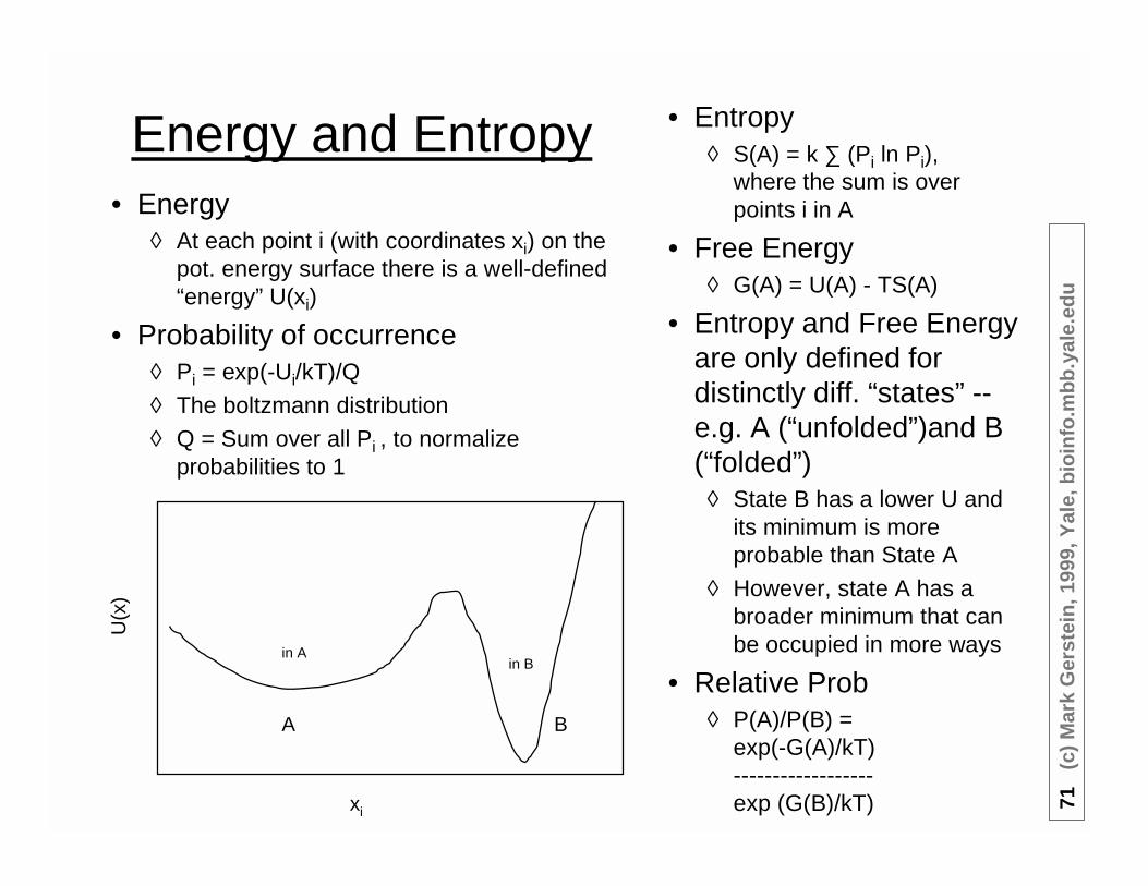
Energy and Entropy• Energy

◊ At each point i (with coordinates xi) on thepot. energy surface there is a well-defined“energy” U(xi)

• Probability of occurrence◊ Pi = exp(-Ui/kT)/Q

◊ The boltzmann distribution◊ Q = Sum over all Pi , to normalize

probabilities to 1

xi

A B

U(x

)

in Ain B

• Entropy◊ S(A) = k ∑ (Pi ln Pi),

where the sum is overpoints i in A

• Free Energy◊ G(A) = U(A) - TS(A)

• Entropy and Free Energyare only defined fordistinctly diff. “states” --e.g. A (“unfolded”)and B(“folded”)

◊ State B has a lower U andits minimum is moreprobable than State A

◊ However, state A has abroader minimum that canbe occupied in more ways

• Relative Prob◊ P(A)/P(B) =

exp(-G(A)/kT)------------------exp (G(B)/kT)

72(c

)M

ark

Ger

stei

n,1

999,

Yal

e,b

ioin

fo.m

bb

.yal

e.ed

u

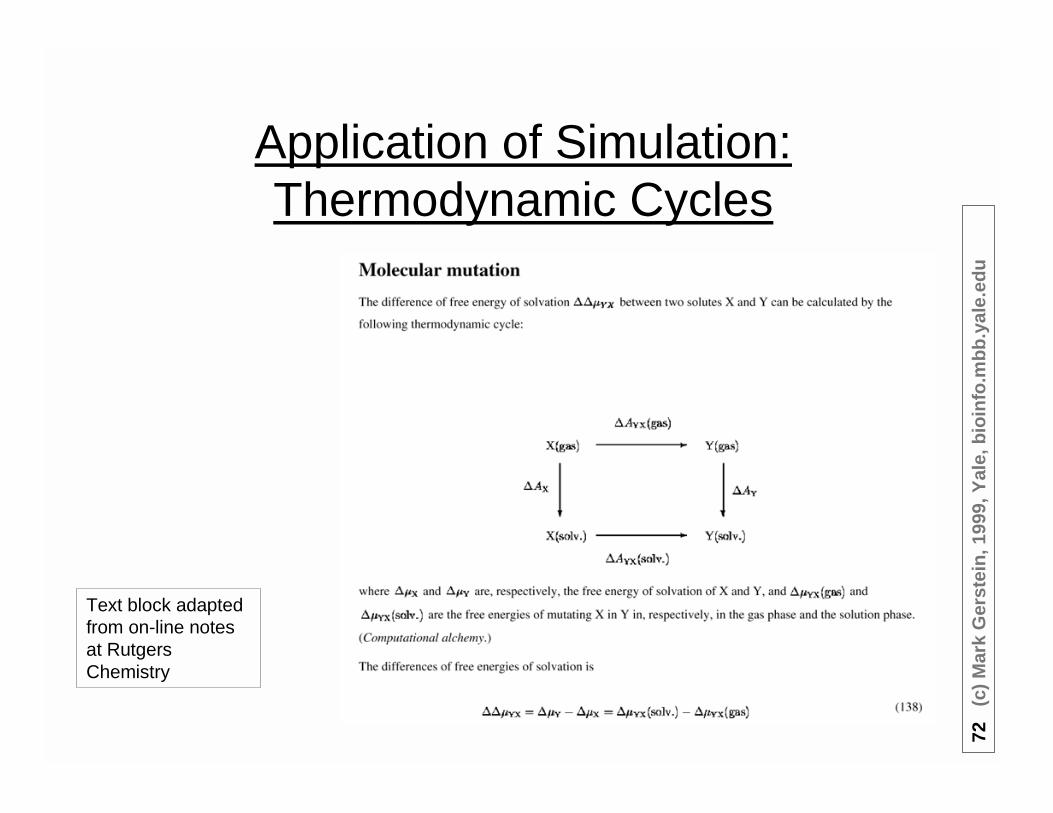
Application of Simulation:Thermodynamic Cycles

Text block adaptedfrom on-line notesat RutgersChemistry

73(c

)M

ark

Ger

stei

n,1

999,

Yal

e,b

ioin

fo.m

bb

.yal

e.ed

u

NumberDensity

= Number of atoms per unit volume averaged over simulation divided bythe number you expect to have in the same volume of an ideal “gas”

Spatially average over all directions gives

1D RDF =

[ Avg. Num. Neighbors at r ][Expected Num. Neighbors at r ]

“at r” means contained in a thin shell of thickness dr and radius r.

74(c

)M

ark

Ger

stei

n,1

999,

Yal

e,b

ioin

fo.m

bb

.yal

e.ed

u

Number Density (cont)• Advantages: Intuitive,

Relates to scattering expts• D/A: Not applicable to real

proteins◊ 1D RDF not structural

◊ 2D proj. only useful with "toy"systems

• Number densitiesmeasure spatialcorrelations, not packing

◊ Low value does not implycavities

◊ Complicated by asymmetricmolecules

◊ How things pack and fit isproperty of instantaneousstructure - not average

75(c

)M

ark

Ger

stei

n,1

999,

Yal

e,b

ioin

fo.m

bb

.yal

e.ed

u

Measurement of Dynamic Quantities I

• The time-course of a relevant variable is characterized by(1) Amplitude (or magnitude), usually characterized by an RMS value

R = sqrt[ < (a(t) - <a(t)>)2 > ]R = sqrt[ < a(t)2 - 2a(t)<a(t)> +<a(t)>2 > ]R = sqrt[ < a(t)2> - <a(t)>2 ]

• similar to SD

• fluctuation

• Relevant variables include bond length, solvent molecule position,H-bond angle, torsion angle

Illustration from M Levitt,Stanford University

76(c

)M

ark

Ger

stei

n,1

999,

Yal

e,b

ioin

fo.m

bb

.yal

e.ed

u

Measurement of Dynamic Quantities II

• The time-course of a relevant variable is characterized by(2) Rate or time-constant

◊ Time Correlation function

◊ CA(t) = <A(s)A(t+s)> = <A(0)A(t)> [ averaging over all s ]

◊ Correlation usually exponentially decays with time t◊ decay constant is given by the integral of C(t) from t=0 to t=infinity

• Relevant variables include bond length, solvent molecule position,H-bond angle, torsion angle


77(c

)M

ark

Ger

stei

n,1

999,

Yal

e,b

ioin

fo.m

bb

.yal

e.ed

u

D & RMS

• Diffusion constant◊ Measures average rate of

increase in variance of position ofthe particles

◊ Suitable for liquids, not really forproteins

D =∆r 2

6∆t

RMS (t ) =di (t )

i =1

N∑N

di (t ) = R(xi (t ) − T) − xi (0)

• RMS more suitable toproteins

◊ di = Difference in position ofprotein atom at t from the initialposition, after structures havebeen optimally rotated translatedto minimize RMS(t)

◊ Solution of optimal rotation hasbeen solved a number of ways(Kabsch, SVD)

78(c

)M

ark

Ger

stei

n,1

999,

Yal

e,b

ioin

fo.m

bb

.yal

e.ed

u

ObservedRMS values


79(c

)M

ark

Ger

stei

n,1

999,

Yal

e,b

ioin

fo.m

bb

.yal

e.ed

u

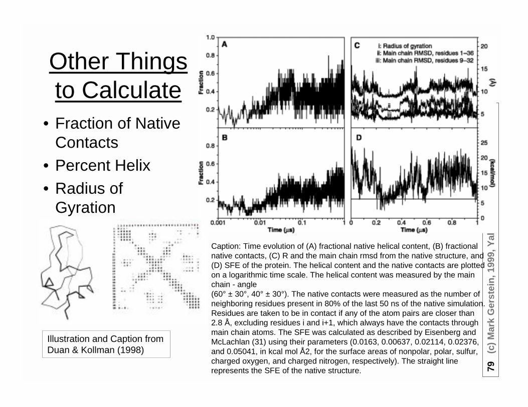
Other Thingsto Calculate

• Fraction of NativeContacts

• Percent Helix• Radius of

Gyration

Illustration and Caption fromDuan & Kollman (1998)

Caption: Time evolution of (A) fractional native helical content, (B) fractionalnative contacts, (C) R and the main chain rmsd from the native structure, and(D) SFE of the protein. The helical content and the native contacts are plottedon a logarithmic time scale. The helical content was measured by the mainchain - angle(60° ± 30°, 40° ± 30°). The native contacts were measured as the number ofneighboring residues present in 80% of the last 50 ns of the native simulation.Residues are taken to be in contact if any of the atom pairs are closer than2.8 Å, excluding residues i and i+1, which always have the contacts throughmain chain atoms. The SFE was calculated as described by Eisenberg andMcLachlan (31) using their parameters (0.0163, 0.00637, 0.02114, 0.02376,and 0.05041, in kcal mol Å2, for the surface areas of nonpolar, polar, sulfur,charged oxygen, and charged nitrogen, respectively). The straight linerepresents the SFE of the native structure.

80(c

)M

ark

Ger

stei

n,1

999,

Yal

e,b

ioin

fo.m

bb

.yal

e.ed

u

MonitorStability of

SpecificHydrogen

Bonds


81(c

)M

ark

Ger

stei

n,1

999,

Yal

e,b

ioin

fo.m

bb

.yal

e.ed

u

Energy Landscapes and BarriersTraversed in a Simulation

Illustrations from M Levitt, Stanford University

82(c

)M

ark

Ger

stei

n,1

999,

Yal

e,b

ioin

fo.m

bb

.yal

e.ed

uTimescales

Motion length time

(Å) (fs)

bond vibration 0.1 10

water hindered rotation 0.5 1000

surface sidechain rotation 5 105

water diffusive motion 4 105

buried sidechain libration 0.5 105

hinge bending of chain 3 106

buried sidechain rotation 5 1013

allosteric transition 3 1013

local denaturation 7 1014

Values fromMcCammon &Harvey (1987) andEisenberg &Kauzmann

83(c

)M

ark

Ger

stei

n,1

999,

Yal

e,b

ioin

fo.m

bb

.yal

e.ed

u

Electrostatics Revisited:the Poisson-Boltzmann Equation

84(c

)M

ark

Ger

stei

n,1

999,

Yal

e,b

ioin

fo.m

bb

.yal

e.ed

u

Poisson-Boltzmann equation

• Macroscopic dielectric◊ As opposed to microscopic one

as for realistic waters

• Linearized: sinh φ = φ◊ counter-ion condense

• The model◊ Protein is point charges embedded in

a low dielectric.

◊ Boundary at accesible surface

◊ Discontinuous change to a newdielectric(no dipoles, no smoothly varying

dielectric)

85(c

)M

ark

Ger

stei

n,1

999,

Yal

e,b

ioin

fo.m

bb

.yal

e.ed

u

Simplifications ofthe Poisson-Boltzmannequation

• Laplace eq.◊ div grad V = ρ◊ grad V = E field◊ Only have divergence when have

charge source

86(c

)M

ark

Ger

stei

n,1

999,

Yal

e,b

ioin

fo.m

bb

.yal

e.ed

u

Protein ona Grid

For intuition ONLY -- Don’tneed to know in detail!!

87(c

)M

ark

Ger

stei

n,1

999,

Yal

e,b

ioin

fo.m

bb

.yal

e.ed

u

Demand Consistency on the Grid

For intuition ONLY-- Don’t need toknow in detail!!


Adding

aD

ielectricB

oundaryinto

theM

odel

89(c

)M

ark

Ger

stei

n,1

999,

Yal

e,b

ioin

fo.m

bb

.yal

e.ed

u

Electrostatic Potentialof Thrombin

The proteolytic enzyme Thrombin (dark backbone worm)complexed with an inhibitor, hirudin (light backbone worm). Thenegatively charged (Light gray) and positively charged (darkgray) sidechains of thrombin are shown in bond representation.

Solvent accessible surface of thrombin coded by electrostaticpotential (dark: positive, light: negative). Hirudin is shown as alight backbone worm. Potential is calculated at zero ionic strength.

Illustration Credit: Sharp (1999)Text captions also from Sharp (1999)

Graphical analysis of electrostatic potential distributions oftenreveals features about the structure that complement analysisof the atomic coordinates. For example, LEFT shows thedistribution of charged residues in the binding site of theproteolytic enzyme thrombin. RIGHT shows the resultingelectrostatic potential distribution on the protein surface. Thebasic (positive) region in the fibrinogen binding, while it couldbe inferred from close inspection of the distribution of chargedresidues in TOP, is more apparent in the potential distribution.

90(c

)M

ark

Ger

stei

n,1

999,

Yal

e,b

ioin

fo.m

bb

.yal

e.ed

u

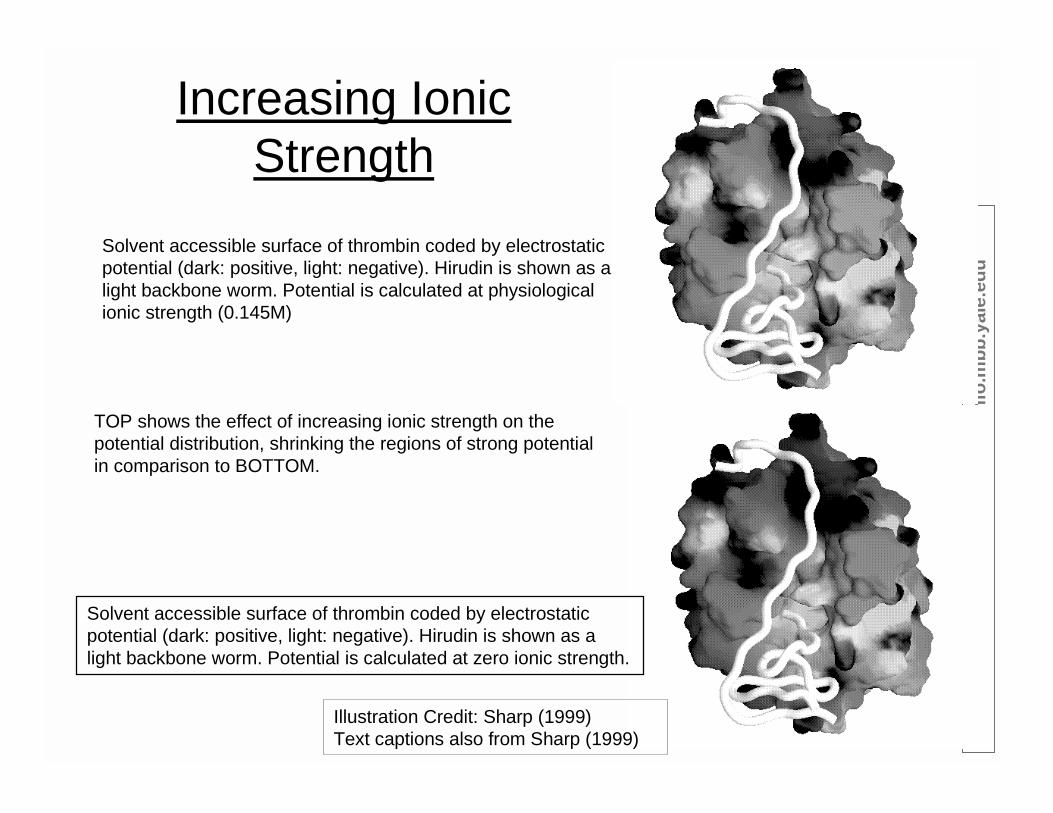
Increasing IonicStrength

Solvent accessible surface of thrombin coded by electrostaticpotential (dark: positive, light: negative). Hirudin is shown as alight backbone worm. Potential is calculated at physiologicalionic strength (0.145M)



TOP shows the effect of increasing ionic strength on thepotential distribution, shrinking the regions of strong potentialin comparison to BOTTOM.

91(c

)M

ark

Ger

stei

n,1

999,

Yal

e,b

ioin

fo.m

bb

.yal

e.ed

u

Increasing Dielectric

Solvent accessible surface of thrombin coded by electrostaticpotential (dark: positive, light: negative). Hirudin is shown as alight backbone worm. Potential is calculated using the samepolarizability for protein and solvent.



TOP is calculated assuming the same dielectric for the solventand protein. The more uniform potential distribution comparedto BOTTOM shows the focusing effect that the low dielectricinterior has on the field emanating from charges in active sitesand other cleft regions.

92(c

)M

ark

Ger

stei

n,1

999,

Yal

e,b

ioin

fo.m

bb

.yal

e.ed

u

pKashifts

Charge transfer processes are important in protein catalysis, binding, conformational

changes and many other functions. The primary examples are acid-base equilibria,

electron transfer and ion binding, in which the transferred species is a proton, an electron

or a salt ion respectively. The theory of the dependence of these three equilibria within

the classical electrostatic framework can be treated in an identical manner, and will be

illustrated with acid-base equilibria. A titratable group will have an intrinsic ionizationequilibrium, expressed in terms of a known intrinsic pKoa. Where pKoa = -log10(Koa),

Koa is the dissociation constant for the reaction H+A = H++A and A can be an acid or a

base. The pKoa is determined by all the quantum chemical, electrostatic and

environmental effects operating on that group in some reference state. For example a

reference state for the aspartic acid side-chain ionization might be the isolated amino

acid in water, for which pKoa = 3.85. In the environment of the protein the pKa will be

altered by three electrostatic effects. The first occurs because the group is positioned in a

protein environment with a different polarizability, the second is due to interaction with

permanent dipoles in the protein, the third is due to charged, perhaps titratable, groups.

The effective pKa is given by (where the factor of 1/2.303kT converts units of energy to

units of pKa):

pKa = pKoa + (∆∆Grf+∆∆Gperm+∆∆Gtit)/2.303kTText block fromSharp (1999) 1. Desolvation,

Rx Field2. PermanentDipoles

3. OtherCharges

93(c

)M

ark

Ger

stei

n,1

999,

Yal

e,b

ioin

fo.m

bb

.yal

e.ed

u

pKacontinued I

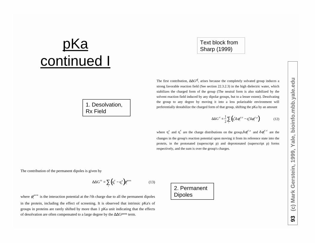
The first contribution, ∆∆Grf, arises because the completely solvated group induces a

strong favorable reaction field (See section 22.3.2.3) in the high dielectric water, which

stabilizes the charged form of the group (The neutral form is also stabilized by the

solvent reaction field induced by any dipolar groups, but to a lesser extent). Desolvating

the group to any degree by moving it into a less polarizable environment will

preferentially destabilize the charged form of that group, shifting the pKa by an amount

∆∆G rf =1

2qi

d∆φi

rf,d − qi

p∆φi

rf ,p( )i

∑ (12)

where qi

pand qi

dare the charge distributions on the group,∆φ

i

rf, pand ∆φ

i

rf, dare the

changes in the group's reaction potential upon moving it from its reference state into the

protein, in the protonated (superscript p) and deprotonated (superscript p) forms

respectively, and the sum is over the group's charges.

The contribution of the permanent dipoles is given by

∆∆G tit = qid − q

i

p( )i

∑ φi

perm (13)

where φi

perm is the interaction potential at the i'th charge due to all the permanent dipoles

in the protein, including the effect of screening. It is observed that intrinsic pKa's of

groups in proteins are rarely shifted by more than 1 pKa unit indicating that the effects

of desolvation are often compensated to a large degree by the ∆∆Gperm term.

1. Desolvation,Rx Field

2. PermanentDipoles

Text block fromSharp (1999)

94(c

)M

ark

Ger

stei

n,1

999,

Yal

e,b

ioin

fo.m

bb

.yal

e.ed

u

pKa continued II

The final term accounts for the contribution of all the other charge groups:

∆∆G titr = qid < φ

i>pH,c, ∆V

d −qi

p < φi

>pH, c, ∆V

p( )i

∑ (14)

where < φi

> is the mean potential at group charge i from all the other titratable groups.

The charge state of the other groups in the protein depend in turn on their intrinsic

"pKa's", on the external pH if they are acid-base groups, the external redox potential ∆V

if they are redox groups, and the concentration of ions, c, if they are ion binding sites, asindicated by the subscript on <φi>. Moreover, the charge state of the group itself will

affect the equilibrium at the other sites. Because of this linkage, exact determination of

the complete charged state of a protein is a complex procedure. If there are N such

groups, the rigorous approach is to compute the titration state partition function by

evaluating the relative electrostatic free energies of all 2N ionization states for a given

set of pH, c, ∆V. From this one may calculate the mean ionization state of any group as a

function of pH, ∆V etc. For large N this becomes impractical, but various approximate

schemes work well, including a Monte-Carlo procedure

3. OtherCharges

Text block fromSharp (1999)


Water

Sim

ulationand

Hydrophobicity

96(c

)M

ark

Ger

stei

n,1

999,

Yal

e,b

ioin

fo.m

bb

.yal

e.ed

u

SimulatingLiquidWater

Illustrations fromM Levitt, StanfordUniversity

97(c

)M

ark

Ger

stei

n,1

999,

Yal

e,b

ioin

fo.m

bb

.yal

e.ed

u

Periodic Boundary Conditions

• Makesimulationsystem seemlarger than it is

• EwaldSummation forelectrostatics(Fouriertransform)

98(c

)M

ark

Ger

stei

n,1

999,

Yal

e,b

ioin

fo.m

bb

.yal

e.ed

u

TetrahedralGeometry of Water

HYDROGEN BONDS give water its uniqueproperties. The hydrogen bond is a consequence ofthe electrical attraction between the positivelycharged hydrogen on one water molecule (H1) andthe negatively charged oxygen on another watermolecule (O’). The electrostatic repulsion betweenthis oxygen and the oxygen that the hydrogen iscovalently bonded to (O) gives the hydrogen bond anearly linear geometry. Each water molecule can actas a donor of two hydrogen bonds to neighboringwater oxygens. Each water can also accept twohydrogen bonds. This double-donor, double-acceptor situation naturally tends to favor atetrahedral geometry with four waters around eachwater oxygen, as shown. Ice has this perfecttetrahedral geometry. However, in water, thetetrahedral geometry is distorted, and it is possiblefor a water molecule to accept or donate more thantwo hydrogen bonds (which are consequently highlydistorted). Such a distortions of tetrahedral geometryare shown, which is taken from a frame in asimulation. Note that the central water moleculeaccepts three hydrogen bonds.

99(c

)M

ark

Ger

stei

n,1

999,

Yal

e,b

ioin

fo.m

bb

.yal

e.ed

u

HydrophobicityArises

Naturallyin Simulation

• Add no hydrophobicEffect◊ This arises naturally

from entropic effectsduring the simulation

M ix in g is a sp o n ta n e o u s p ro c e s s : a s u b s ta n c e w ill n a tu ra l lyd is s o lv e in w a te r u n le ss th e re a re m a n ife s t ly u n fa v o ra b le in te ra c tio n sb e tw e e n it a n d w a te r . S c ie n tis ts u su a lly d is c u s s th e fa v o ra b le n e s s o fp a r t ic u la r in te ra c tio n s in te rm s o f th e e n e rg y a s so c ia te d w ith th ein te rm o le c u la r fo rc e s . A lm o s t a lw a y s th e re a re a t le a s t s o m e e n e rg e tic a l lyfa v o ra b le d is p e r s io n in te ra c tio n s b e tw e e n th e s o lu te a n d th e w a te r .H o w e v e r , th e m o re s a lie n t is s u e is h o w th e in te ra c tio n b e tw e e n a s o lu tea n d a w a te r m o le c u le c o m p a r e s in s tre n g th to th e in te ra c tio n b e tw e e n tw ow a te r m o le c u le s o r b e tw e e n tw o s o lu te m o le c u le s . F o r in s ta n c e , a p o la rm o le c u le s u c h a s g lu c o s e is a b le to m a k e c o m p a ra b le h y d ro g e n b o n d s tow a te r a s w a te r m o le c u le s c a n m a k e w ith e a c h o th e r . T h u s , th e re a re n ou n fa v o ra b le in te ra c tio n s p re v e n tin g it f ro m d is s o lv in g a n d it is v e rys o lu b le .

In c o n tra s t , w a te r m o le c u le s a re n o t a b le to h y d ro g e n b o n d tom e th a n e , a n in so lu b le , n o n -p o la r so lu te . T h e y w o u ld ra th e r in te ra c t w ithe a c h o th e r . T h e m e th a n e m o le c u le s , m o re o v e r , c a n fa v o ra b ly in te ra c tw ith e a c h o th e r th ro u g h a ttra c t iv e d isp e rs io n fo rc e s . O n e c a n s e e h o w th iss i tu a tio n le a d s to m e th a n e m o le c u le s try in g to m in im iz e th e ir r e la tiv e lyu n fa v o ra b le in te ra c tio n s w ith w a te r m o le c u le s . A n o b v io u s w a y th e y c a nd o th is is b y c lu m p in g to g e th e r , a g g re g a tin g , a n d c o m in g o u t s o lu tio n .S u c h a g g re g a tio n o f n o n -p o la r s o lu te s in w a te r is o f te n c a lle d th eh y d r o p h o b ic e ffe c t a n d , a s w e s h a ll , i t is v e ry im p o rta n t inm a c ro m o le c u la r s tru c tu re .

In te rm s o f w a te r s tru c tu re a t ro o m te m p e ra tu re , th e re la t iv e lyu n fa v o ra b le in te ra c tio n b e tw e e n w a te r a n d m e th a n e in d u c e s e a c h w a te rm o le c u le n e x t to m e th a n e to “ tu rn a w a y ” f ro m it a n d h y d ro g e n b o n d ton e ig h b o r in g w a te r m o le c u le s . I f o n e o f th e se tu rn e d w a te r m o le c u le sm a n a g e s to k e e p itse lf c o rre c tly o r ie n te d o v e r t im e , i t w ill h a v e w ill n o th a v e to s a c r if ic e a n y o f i ts u s u a l fo u r to f iv e h y d ro g e n b o n d s . T h is b r in g su p a n in te re s t in g p a ra d o x : F ro m th e s ta n d p o in t o f fa v o ra b le in te ra c tio n s ,o r e n e rg y in m o re fo rm a l te rm in o lo g y , w a te r h a s n o t p a id a n y p r ic e ins o lv a tin g th e m e th a n e . C o n se q u e n tly , th e re a p p e a r s to b e n o e n e rg e ticre a s o n fo r m e th a n e to b e in so lu b le in w a te r .

T h is p a ra d o x is re s o lv e d b y e n tro p y . A c c o rd in g to o n e w a y o fth in k in g , e n tro p y re f le c ts th e n u m b e r o f p o s s ib le s ta te s a m o le c u le c a ne x is t in . T h u s , th e m o re s ta te s a w a te r m o le c u le c a n e x is t in , th e b e tte r i tss i tu a tio n is e n tro p ic a lly , a n d if a s o lu te “ p in s d o w n ” a w a te r m o le c u le o rre s tr ic ts i ts f r e e d o m o f m o tio n , i t is e n tro p ic a lly u n fa v o ra b le . A ll s o lu te sre s tr ic t th e f re e d o m o f m o tio n o f w a te r m o le c u le s to s o m e d e g re e , b u tth is is p a r t ic u la r ly tru e fo r a n o n -p o la r so lu te , su c h a s m e th a n e . T h u s ,s in c e tu rn in g a w a y fro m m e th a n e “ p in s d o w n ” e a c h w a te r m o le c u les l ig h tly , th e p r ic e o f h y d ra tin g th is n o n -p o la r s o lu te is p a id in d ire c tly inte rm s o f e n tro p y a n d n o t d ire c tly in te rm s o f e n e rg y .

T h e h y d ro p h o b ic e ffe c t is c u rre n tly re c e iv in g in te n se s c ru tin y fro ms im u la tio n a n d e x p e r im e n t. T h e p ic tu re th a t is e m e rg in g is s o m e w h a tm o re c o m p lic a te d th a n th e s im p lif ie d a c c o u n t p re s e n te d h e re s in c e a th ig h te m p e ra tu re s , h y d ro p h o b ic h y d ra tio n is s t i l l u n fa v o ra b le b u t fo re n e rg e tic a n d n o t e n tro p ic re a s o n s . N e v e r th e le s s , ir r e sp e c tiv e o f w h e th e rth e p r ic e is p a id in te rm s o f e n e rg y o r e n tro p y , th e h y d ro p h o b ic e ffe c t isfu n d a m e n ta lly c a u s e d b y th e r e la tiv e ly u n fa v o ra b le in te ra c tio n s b e tw e e nw a te r a n d h y d ro p h o b ic s o lu te s .

100

(c)

Mar

kG

erst

ein

,199

9,Y

ale,

bio

info

.mb

b.y

ale.

edu

Different Behavior of Water aroundHydrophobic and Hydrophilic Solutes

POLAR AND NON-POLAR SOLUTES have very different effects on water structure. We show two solutesthat have the same Y-shaped geometry but different partial charges. The polar solute, urea (left), has partialcharges on its atoms. Consequently, it is able hydrogen-bond to water molecules and to fit right into the waterhydrogen-bond network. In contrast, the non-polar solute, isobutene (right), does not have (substantial) partialcharges on any of its atoms. It, thus, can not hydrogen-bond to water. Rather, the water molecules around it“turn away” and interact strongly only with other water molecules, forming a sort of hydrogen-bond “cage”around the isobutene.

101

(c)

Mar

kG

erst

ein

,199

9,Y

ale,

bio

info

.mb

b.y

ale.

edu

Consequences of HydrophobicHydration and “Clathrate” Formation

• Hydrophobic hydration is unfavorable (G) but thereason is different at different T◊ entropically (S) unfavorable at low temperatures because of ordering◊ enthalpically (H) unfavorable at high temperatures because of

unsatisified H-bonds

• Volume of mixing is negative• Compressibility• High heat capacity of hydrophobic solvation

◊ Signature of hydrophobic hydration◊ Hydration creates new temperature “labile” structures


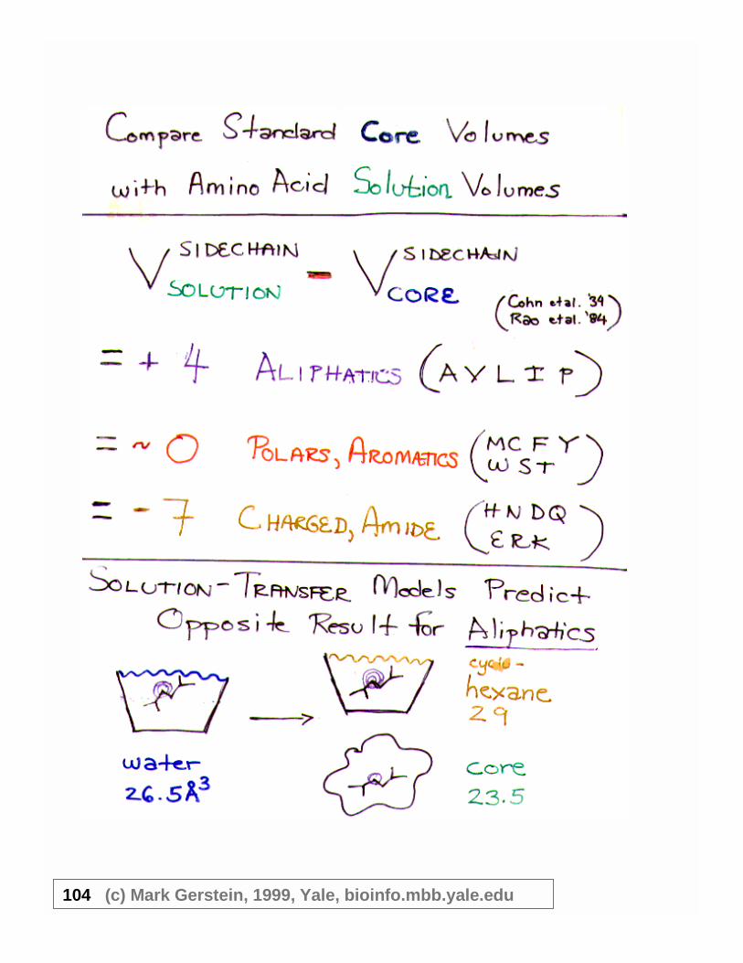
Ways

ofRationalizing

Packing

105

(c)

Mar

kG

erst

ein

,199

9,Y

ale,

bio

info

.mb

b.y

ale.

edu

Water around Hydrophobic Groups onprotein surface is more Compressible

• Fluctuations in polyhedra volume over simulationrelated to compressibility◊ Same way amplitude of a spring is related to spring constant◊ Rigorous for NPT only, approximately true for part of NVE

• Simulation Results (avg. fluctuations as %SD andcompressibility)◊ Protein core 9.7 % .14

◊ Protein surface 11.7 % .29◊ Water near protein 13.2 % .50

◊ Bulk water 11.9 % .41

◊ Consistent with more variable packing at protein surface

• Results verified by doing high-pressure simulation(5000 atm, 10000 atm)◊ Allows calculation of compressibility from definition

106

(c)

Mar

kG

erst

ein

,199

9,Y

ale,

bio

info

.mb

b.y

ale.

edu

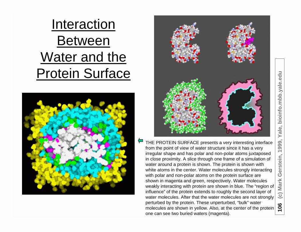
InteractionBetween

Water and theProtein Surface

THE PROTEIN SURFACE presents a very interesting interfacefrom the point of view of water structure since it has a veryirregular shape and has polar and non-polar atoms juxtaposedin close proximity. A slice through one frame of a simulation ofwater around a protein is shown. The protein is shown withwhite atoms in the center. Water molecules strongly interactingwith polar and non-polar atoms on the protein surface areshown in magenta and green, respectively. Water moleculesweakly interacting with protein are shown in blue. The “region ofinfluence” of the protein extends to roughly the second layer ofwater molecules. After that the water molecules are not stronglyperturbed by the protein. These unperturbed, “bulk” watermolecules are shown in yellow. Also, at the center of the proteinone can see two buried waters (magenta).

107

(c)

Mar

kG

erst

ein

,199

9,Y

ale,

bio

info

.mb

b.y

ale.

edu

Simple Two Helix System

• Number density

◊ g = Normalwater,straight &helical projections

◊ For usual RDF“volume elements”are concentricspherical shells

◊ Here, they are tinyvertical columns andhelicesperpendicular topage

◊ More intuition aboutgroove expansion

• Compare waterpacking with that ofsimple liquid (“re-scaled Ar”)


Second

SolventS

hell:W

aterv

LJLiquid


Watervs.A

r

(Helical

Project-ions)

110

(c)

Mar

kG

erst

ein

,199

9,Y

ale,

bio

info

.mb

b.y

ale.

edu

Hydration Surface

• Bring together two helices◊ Unusually low water density in grooves and crevices — especially, as

compared to uncharged water

◊ Fit line through second shell

111

(c)

Mar

kG

erst

ein

,199

9,Y

ale,

bio

info

.mb

b.y

ale.

edu

Water Participatesin Protein Unfolding

A PROTEIN HELIX CAN UNFOLD more easily in solution (than in vacuum) because watermolecules can replace its helical hydrogen bonds. An unfolding helix is shown. The bottomhalf the helix is intact and has its helical hydrogen bonds while the top half is unfolded. Inthe middle a water molecule (green) is shown bridging between two atoms that would behydrogen-bonded in a folded helix: the carbonyl oxygen (red) and the amide nitrogen(blue).


Sim

plifiedS

imulation

113

(c)

Mar

kG

erst

ein

,199

9,Y

ale,

bio

info

.mb

b.y

ale.

edu

Simplification


114

(c)

Mar

kG

erst

ein

,199

9,Y

ale,

bio

info

.mb

b.y

ale.

edu

SimplifiedProtein:LatticeModels

• CubicLattice

• Tetra-hedralLattice


Illustration fromDill et al. (1990)

115

(c)

Mar

kG

erst

ein

,199

9,Y

ale,

bio

info

.mb

b.y

ale.

edu

Off-latticeDiscrete State

Models

Illustration from M Levitt, Stanford University

116

(c)

Mar

kG

erst

ein

,199

9,Y

ale,

bio

info

.mb

b.y

ale.

edu

How Well Do Lattice StructuresMatch Real Protein Structure?

Illustration Credit: Dill et al. (1995)

Illustration Credit: Hinds & Levitt (1992)

117

(c)

Mar

kG

erst

ein

,199

9,Y

ale,

bio

info

.mb

b.y

ale.

edu

How well doesthe off-lattice

model fit?

ModelComplexity vsFit to Reality


118

(c)

Mar

kG

erst

ein

,199

9,Y

ale,

bio

info

.mb

b.y

ale.

edu

Simplified Solvent

Figures from Smit et al. (1990)

• Smit et al. (1990) Surfactantsimulation

• Three types of particles, o, wand s◊ s consists of

w-w-o-o-o-o

◊ s has additional springs

• all particles interact through L-Jpotential◊ o-w interaction truncated so purely

repulsive

• Above sufficient to give rise tothe formation of micelles,membranes, &c

119

(c)

Mar

kG

erst

ein

,199

9,Y

ale,

bio

info

.mb

b.y

ale.

edu

Review -- Basic Forces• Basic Forces

◊ Springs --> Bonds

◊ Electrical

• dipoles and induced dipoles --> VDW force --> Packing• unpaired charges --> Electrostatics --> charge-charge

• Electrostatics◊ All described the PBE

◊ kqQ/r -- the simplest case for point charges

• Multipoles for more complex dist.• Validity of monopole or dipole Apx. (helix dipole?)

◊ Polarization (epsilon)

• Qualitative understanding of what it does• 80 vs 3

120

(c)

Mar

kG

erst

ein

,199

9,Y

ale,

bio

info

.mb

b.y

ale.

edu

Review -- Simulation

• Moving on an Energy Landscape◊ Minimization -- steepest descent

◊ Monte Carlo◊ Molecular Dynamics

• Know how an atom will move◊ The problems

• Too complex --> Simplified Models• Potential Problems

• Analysis◊ Number density --> RDF, structural quantities

◊ Dynamic quantities, correlation functions, diffusion

• time course of variables◊ Hydrophobicity arises naturally in water simulation

• clathrate formation• high heat capacity, volume effects, &c.

121

(c)

Mar

kG

erst

ein

,199

9,Y

ale,

bio

info

.mb

b.y

ale.

edu

Demos

• Minimization Demo◊ http://www.javasoft.com/applets/jdk/1.0/demo/GraphLayout/example2.html

• Adiabatic Mapping Demo◊ Molecular Motions Database

◊ http://bioinfo.mbb.yale.edu/MolMovDB

• Rotation Matrices, Rigid Body Motion Demo◊ 1swm, 2hbs, rasmol

122

(c)

Mar

kG

erst

ein

,199

9,Y

ale,

bio

info

.mb

b.y

ale.

edu

References

• Allen, M. P. & Tildesley, D. J. (1987). ComputerSimulation of Liquids. Claredon Press, Oxford

• Brooks, B. R., Bruccoleri, R. E., Olafson, B. D.,States, D. J., Swaminathan, S. & Karplus, M.(1983). CHARMM: A Program for MacromolecularEnergy, Minimization, and Dynamics Calculations.J. Comp. Chem. 4, 187-217.

• Daggett, V. & Levitt, M. (1993). RealisticSimulations of Native-Protein Dynamics inSolution and Beyond. Ann. Rev. Biophys. Biomol.Struct. 22, 353-380.

• Dill, K. A., Bromberg, S., Yue, K., Fiebig, K. M.,Yee, D. P., Thomas, P. D. & Chan, H. S. (1995).Principles of protein folding--a perspective fromsimple exact models. Protein Sci 4, 561-602.

• Duan, Y. & Kollman, P. A. (1998). Pathways to aprotein folding intermediate observed in a 1-microsecond simulation in aqueous solutionScience 282, 740-4.

• Eisenberg, D. & Kauzmann, W. (1969). TheStructure and Properties of Water. ClarendonPress, Oxford.

• Franks, F. (Ed.) (1973). Water: A ComprehensiveTreatise. New York: Plenum Press.

• Franks, F. (1983). Water. The Royal Society ofChemistry, London.

• Gelin, B. R. & Karplus, M. (1979). Side-chaintorsional potentials: effect of dipeptide, protein,and solvent environment. Biochemistry 18, 1256-1268.

• Gerstein, M. & Chothia, C. (1996). Packing at theProtein-Water Interface. Proc. Natl. Acad. Sci.USA 93, 10167-10172.

• Gerstein, M. & Levitt, M. (1998). Simulating Waterand the Molecules of Life. Sci. Am. 279, 100-105.

• Gerstein, M. & Lynden-Bell, R. M. (1993a).Simulation of Water around a Model Protein Helix.2. The Relative Contributions of Packing,Hydrophobicity, and Hydrogen Bonding. J. Phys.Chem. 97, 2991-2999.

• Gerstein, M. & Lynden-Bell, R. M. (1993b). Whatis the natural boundary for a protein in solution? J.Mol. Biol. 230, 641-650.

• Gerstein, M., Tsai, J. & Levitt, M. (1995). Thevolume of atoms on the protein surface:Calculated from simulation, using Voronoipolyhedra. J. Mol. Biol. 249, 955-966.

• Hinds, D. A. & Levitt, M. (1992). A lattice modelfor protein structure prediction at low resolution.Proc Natl Acad Sci U S A 89, 2536-40.

123

(c)

Mar

kG

erst

ein

,199

9,Y

ale,

bio

info

.mb

b.y

ale.

edu

References 2• Honig, B. & Nicholls, A. (1995). Classical

electrostatics in biology and chemistry. Science268, 1144-9.

• Karplus, M. & McCammon, J. A. (1986). Thedynamics of proteins. Sci. Am. 254, 42-51.

• Karplus, M. & Petsko, G. A. (1990). Moleculardynamics simulations in biology. Nature 347, 631-639.

• Levitt, M. (1982). Protein conformation, dynamics,and folding by computer simulation. Ann. Rev.Biophys. Bioeng. 11, 251-271.

• Levitt, M. (1983a). Molecular dynamics of a nativeprotein. I. Computer simulation of trajectories. J.Mol. Biol. 168, 595.

• Levitt, M. (1983b). Molecular dynamics of a nativeprotein. II. Analysis and Nature of the Motion. J.Mol. Biol. 168, 621-657.

• Levitt, M., Hirschberg, M., Sharon, R. & Daggett,V. (1995). Potential Energy Function andParameters for Simulations of the MolecularDynamics of Proteins and Nucleic Acids inSolution. Computer Phys. Comm. 91, 215-231.

• Levitt, M. & Sharon, R. (1988). AccurateSimulation of Protein Dynamics in Solution. Proc.Natl. Acad. Sci. USA 85, 7557-7561.

• McCammon, J. A. & Harvey, S. C. (1987).Dynamics of Proteins and Nucleic Acids.Cambridge UP,

• Park, B. H. & Levitt, M. (1995). The complexityand accuracy of discrete state models of proteinstructure. J Mol Biol 249, 493-507.

• Press, W. H., Flannery, B. P., Teukolsky, S. A. &Vetterling, W. T. (1992). Numerical Recipes in C.Second. Cambridge University Press, Cambridge.

• Pollack, A. (1998). Drug Testers Turn to'VirtualPatients' as Guinea Pigs. New York Times.Nov. 10,

• Press, W. H., Flannery, B. P., Teukolsky, S.A. & Vetterling, W. T. (1992). NumericalRecipes in C. Second. CambridgeUniversity Press, Cambridge.

• Sharp, K. (1999). Electrostatic Interactionsin Proteins. In International Tables forCrystallography, International Union ofCrystallography, Chester, UK.

• Sharp, K. A. & Honig, B. (1990).Electrostatic interactions inmacromolecules. Annu. Rev. Biophys.Biophys. Chem. 19, 301-32

• Smit, B., Hilbers, P. A. J., Esselink, K.,Ruppert, L. A. M., Os, N. M. v. & Schlijper(1990). Computer simulation of a water/oilinterface in the presence of micelles.Nature 348, 624-625.

124

(c)

Mar

kG

erst

ein

,199

9,Y

ale,

bio

info

.mb

b.y

ale.

edu

References

• llen, M. P. & Tildesley, D. J. (1987). ComputerSimulation of Liquids. Claredon Press, Oxford.

• Biosym (1994). Discover 2.9.5 Manual. BiosymInc., San Diego, CA.

• Brooks, B. R., Bruccoleri, R. E., Olafson, B. D.,States, D. J., Swaminathan, S. & Karplus, M.(1983). CHARMM: A Program for MacromolecularEnergy, Minimization, and Dynamics Calculations.J. Comp. Chem. 4, 187-217.

• Daggett, V. & Levitt, M. (1993). RealisticSimulations of Native-Protein Dynamics inSolution and Beyond. Ann. Rev. Biophys. Biomol.Struct. 22, 353-380.

• Gelin, B. R. & Karplus, M. (1979). Side-chaintorsional potentials: effect of dipeptide, protein,and solvent environment. Biochemistry 18, 1256-1268.

• Goldstein, H. (1980). Classical Mechanics. 2ndedition. Addison-Wesley, New York.

• Jackson, J. (1975). Classical Electrodynamics.Wiley, New York.

• Karplus, M. & McCammon, J. A. (1986). Thedynamics of proteins. Sci. Am. 254, 42-51.

• Karplus, M. & Petsko, G. A. (1990). Moleculardynamics simulations in biology. Nature 347, 631-639.

• Levitt, M. (1982). Protein conformation, dynamics,and folding by computer simulation. Ann. Rev.Biophys. Bioeng. 11, 251-271.

• Levitt, M. (1983a). Molecular dynamics of a nativeprotein. I. Computer simulation of trajectories. J.Mol. Biol. 168, 595.

• Levitt, M. (1983b). Molecular dynamics of a nativeprotein. II. Analysis and Nature of the Motion. J.Mol. Biol. 168, 621-657.

• Levitt, M. (1983c). Protein folding by restrainedenergy minimization and molecular dynamics. JMol Biol 170, 723-64.

• Levitt, M., Hirschberg, M., Sharon, R. & Daggett,V. (1995). Potential Energy Function andParameters for Simulations of the MolecularDynamics of Proteins and Nucleic Acids inSolution. Computer Phys. Comm. 91, 215-231.

125

(c)

Mar

kG

erst

ein

,199

9,Y

ale,

bio

info

.mb

b.y

ale.

edu

References 2

• Levitt, M. & Sharon, R. (1988). AccurateSimulation of Protein Dynamics in Solution. Proc.Natl. Acad. Sci. USA 85, 7557-7561.

• Marion, J. B. & Heald, M. A. (1980). ClassicalElectromagnetic Radiation. Academic Press, NewYork.

• McCammon, J. A. & Harvey, S. C. (1987).Dynamics of Proteins and Nucleic Acids.Cambridge UP,

• Pettitt, B. M. & Karplus, M. (1985). The Potentialof Mean Force Surface for the Alanine Dipeptidein Aqeous Solution: A Theoretical Approach.Chem. Phys. Lett. 121, 194-201.

• Atkins, P. (1990). Physical Chemistry.Oxford UP

• Press, W. H., Flannery, B. P., Teukolsky, S. A. &Vetterling, W. T. (1992). Numerical Recipes in C.Second. Cambridge University Press, Cambridge.

• Purcell, E. M. (1985). Electricity and Magnetism.McGraw-Hill, New York.

• Brünger, A. T. (1993). X-PLOR 3.1, A System forX-ray Crystallography and NMR. Yale UniversityPress, New Haven.

• Brünger, A. T., Kuriyan, J. & Karplus, M. (1987).Crystallographic R factor refinement by moleculardynamics. Science 235, 458-60.

• Rice, L. M. & Brunger, A. T. (1996). Torsion angledynamics: Reduced variable conformationalsampling enhances crystallographic structurerefinement. Proteins 19, 277-290

Simulation BIOINFORMATICS - Gerstein Labbioinfo.mbb.yale.edu/mbb452a/simulation/simulation.pdf · 3...

Documents

Transcript of Simulation BIOINFORMATICS - Gerstein Labbioinfo.mbb.yale.edu/mbb452a/simulation/simulation.pdf · 3...