Review of Net Calorific Values for Non-Standard Gaseous Fuels
Simulating the combustion of gaseous fuels6th OpenFoam Workshop Training Session
Dominik Christ
This presentation shows how to use OpenFoam to simulate gas phase combustion
Overview
Theory
Tutorial case
Solution strategies
Validation
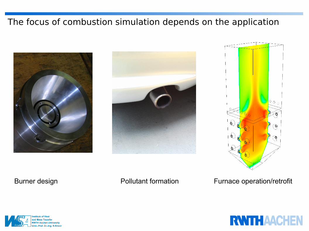
The focus of combustion simulation depends on the application
Furnace operation/retrofitPollutant formationBurner design

The focus of the present tutorial is simulating a model flame
■ Model flames are a basis to test and evaluate combustion solvers
■ Tutorial case is a turbulent methane/air flame(“Flame D” from Sandia/TNF workshop)
■ Solver applications used arerhoReactingFoam (PaSR model)edcSimpleFoam (EDC model)
■ Validation with experimental data to assess the solver/model accuracy
Photo: Sandia/TNF

Overview
Theory (combustion; radiation)
Tutorial case
Solution strategies
Validation
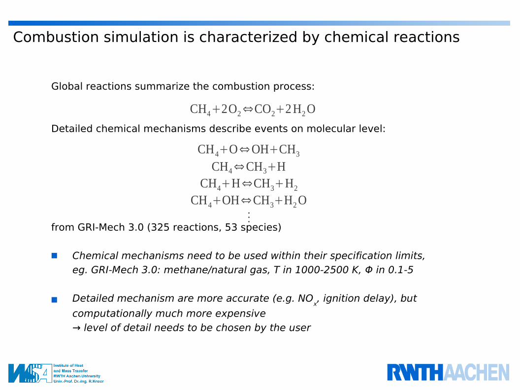
Combustion simulation is characterized by chemical reactions
Global reactions summarize the combustion process:
Detailed chemical mechanisms describe events on molecular level:
from GRI-Mech 3.0 (325 reactions, 53 species)
■ Chemical mechanisms need to be used within their specification limits,eg. GRI-Mech 3.0: methane/natural gas, T in 1000-2500 K, Φ in 0.1-5
■ Detailed mechanism are more accurate (e.g. NOx, ignition delay), but
computationally much more expensive → level of detail needs to be chosen by the user
CH42O2⇔CO22H2O
CH4O⇔OHCH3
CH4⇔CH3HCH4H⇔CH3H2
CH4OH⇔CH3H2O⋮
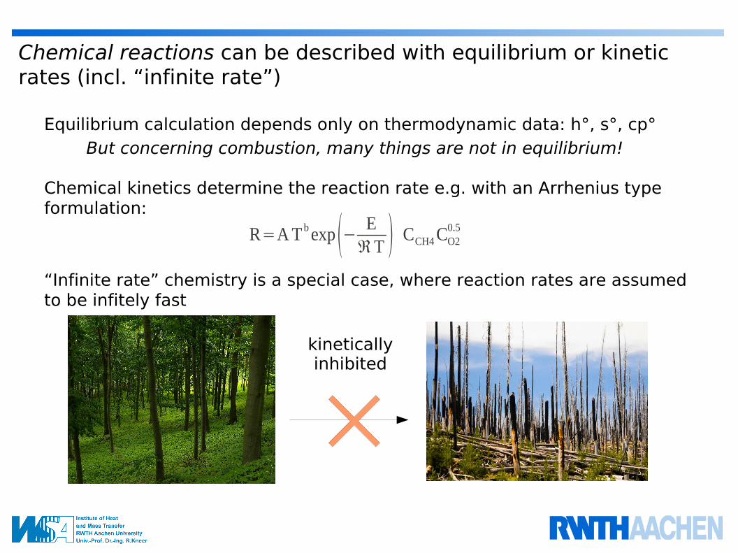
Chemical reactions can be described with equilibrium or kinetic rates (incl. “infinite rate”)
Equilibrium calculation depends only on thermodynamic data: h°, s°, cp°But concerning combustion, many things are not in equilibrium!
Chemical kinetics determine the reaction rate e.g. with an Arrhenius type formulation:
“Infinite rate” chemistry is a special case, where reaction rates are assumed to be infitely fast
kinetically inhibited
R=AT bexp− EℜT CCH4CO2
0.5

In turbulent flows, turbulence/chemistry interaction defines the reacting flow
■ Turbulence enhances mixing of species such as fuel, oxidizer and products
■ Strong turbulence can suppress combustion → local extinction
Turbulent flow Chemical kinetics
■ In a laminar flow, combustion is controlled exclusively by chemical kinetics
■ Combustion leads to flow acceleration → modification of flow field
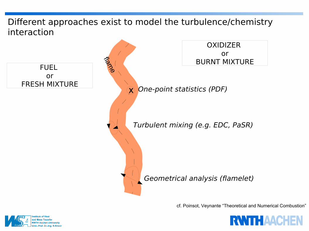
Different approaches exist to model the turbulence/chemistry interaction
cf. Poinsot, Veynante “Theoretical and Numerical Combustion”
x
Turbulent mixing (e.g. EDC, PaSR)
Geometrical analysis (flamelet)
One-point statistics (PDF)
flame FUEL
orFRESH MIXTURE
OXIDIZER or
BURNT MIXTURE
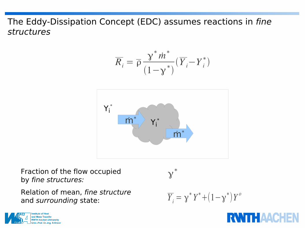
R i = ∗ m∗
1−∗Y i−Y i
∗
The Eddy-Dissipation Concept (EDC) assumes reactions in fine structures
Yi*m∗
m∗
Yi°
Y i = γ∗Y∗
+(1−γ∗)Y oRelation of mean, fine structure
and surrounding state:
Fraction of the flow occupied by fine structures:
∗
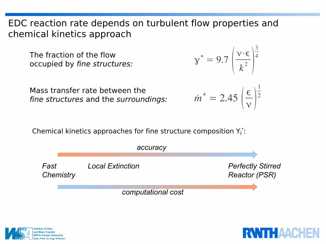
EDC reaction rate depends on turbulent flow properties and chemical kinetics approach
The fraction of the flow occupied by fine structures:
Mass transfer rate between thefine structures and the surroundings:
∗= 9.7 ⋅k 2
34
m∗= 2.45 12
Chemical kinetics approaches for fine structure composition Yi*:
FastChemistry
Local Extinction Perfectly Stirred Reactor (PSR)
accuracy
computational cost
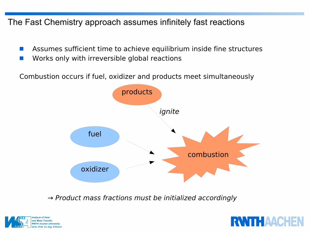
The Fast Chemistry approach assumes infinitely fast reactions
■ Assumes sufficient time to achieve equilibrium inside fine structures■ Works only with irreversible global reactions
Combustion occurs if fuel, oxidizer and products meet simultaneously
→ Product mass fractions must be initialized accordingly
fuel
oxidizer
products
ignite
combustion
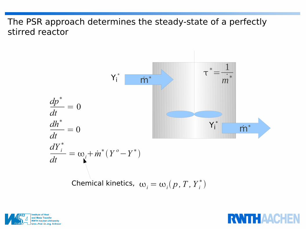
The PSR approach determines the steady-state of a perfectly stirred reactor
dp∗
dt= 0
dh∗
dt= 0
dY i∗
dt=im
∗Y o
−Y ∗
Chemical kinetics, i=i p ,T ,Y i∗
Yi*
m∗
m∗
Yi°
∗=
1m∗

Local Extinction approach employs data from a priori PSR calculations
∗ch ⇒ R=0
τch is the minimum residence time which sustains combustion in PSR.
high turbulence(τ*=2.e-6)
medium turbulence(τ*=2.e-4)
T = 300 K(τch= 1.e-4)
T = 900 K(τch= 2.e-5)
Example 1: Close to burner
Example 2: Free stream reaction zone
<
>

The PaSR combustion model derives the reation rate in a transient manner
Ri=C i ,1−C i ,0
t
Δt
Mixed fraction of cell that can react: κ
C0 C1

The parameter κ is based on two time scales
=ch
mch
1ch
=max − R fuel
Y fuel
,−RO2
Y O2m= k
12
Chemical time scale (infinite or finite rate):Turbulent mixing time scale:
Mixed fraction that reacts:
1ch
=−∂ R∂Y
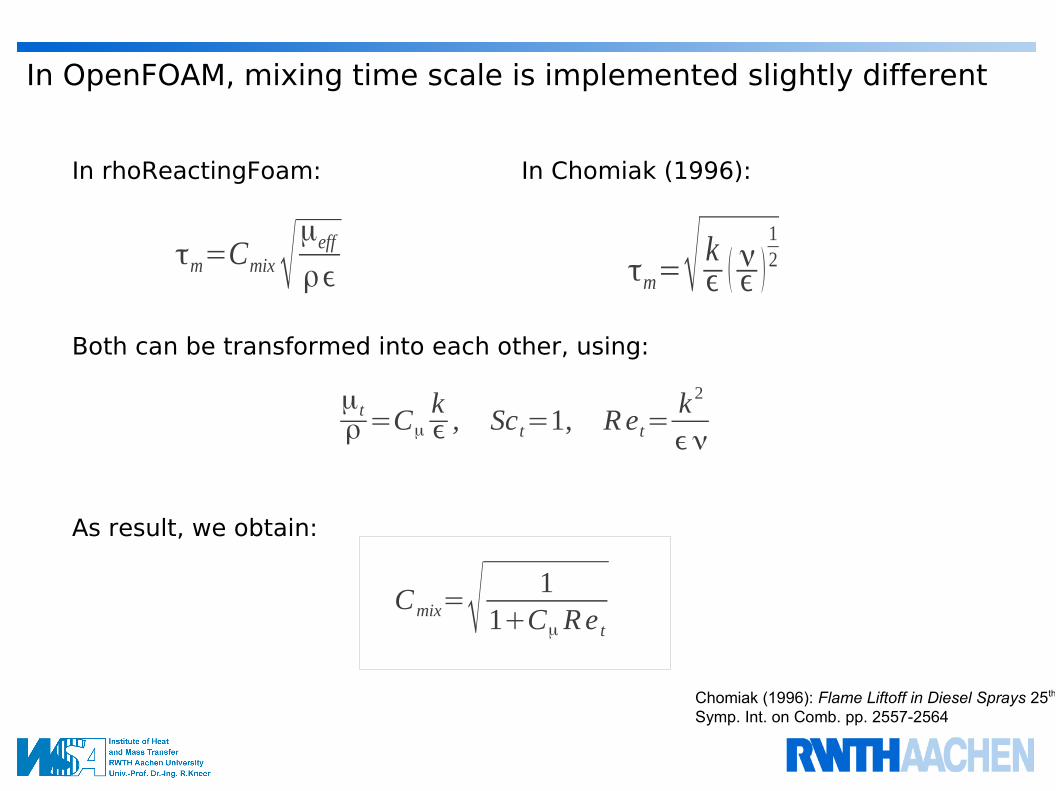
In OpenFOAM, mixing time scale is implemented slightly different
τm=√ kϵ ( νϵ )
12τm=Cmix √
μeff
ρϵ
In rhoReactingFoam: In Chomiak (1996):
Both can be transformed into each other, using:
μtρ =Cμ
kϵ , Sct=1, Ret=
k 2
ϵ ν
As result, we obtain:
Cmix=√ 11+Cμ Re t
Chomiak (1996): Flame Liftoff in Diesel Sprays 25th Symp. Int. on Comb. pp. 2557-2564
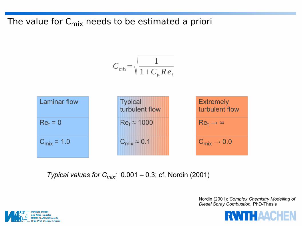
The value for Cmix needs to be estimated a priori
Typical turbulent flow
Ret ≈ 1000
Cmix ≈ 0.1
Laminar flow
Ret = 0
Cmix = 1.0
Extremely turbulent flow
Ret → ∞
Cmix → 0.0
Cmix=√ 11+Cμ Re t
Nordin (2001): Complex Chemistry Modelling of Diesel Spray Combustion, PhD-Thesis
Typical values for Cmix: 0.001 – 0.3; cf. Nordin (2001)

Radation heat transfer needs to be considered in combustion simulation
Radiation Transport Equation:
P1 - Transport
Discrete Ordinates (DOM)
Gas-Absorption Modelling:
constant
RADCAL-Polynomials
WSGGM (custom)
Peak temperature ≈250 K higher without radiation modelling
Overview
Theory
Tutorial case
Solution strategies
Validation

The tutorial case is a non-premixed piloted flame (“Flame D”)
Characteristics: Steady-state, piloted, methane/air, diffusion flame, some local extinction
Geometry:Axi-symmetric, 2D
Main jet (CH4/air)
Pilot (hot flue gas)
Coflow (air)
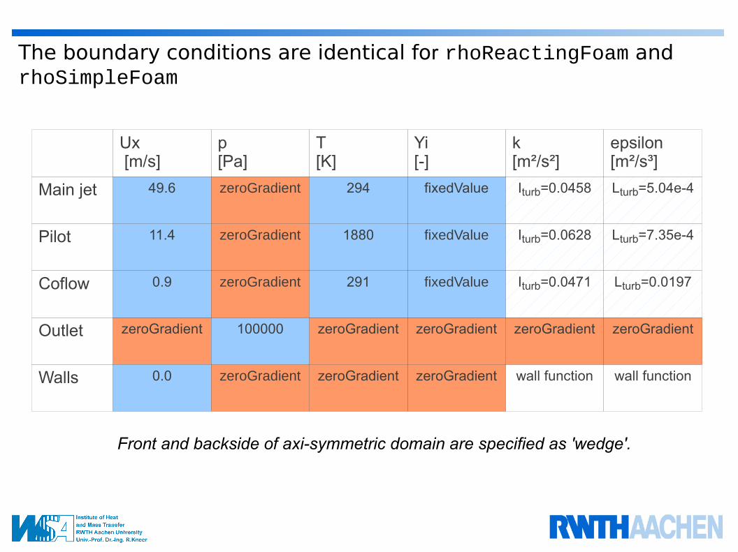
The boundary conditions are identical for rhoReactingFoam and rhoSimpleFoam
Ux [m/s]
p[Pa]
T[K]
Yi[-]
k[m²/s²]
epsilon[m²/s³]
Main jet 49.6 zeroGradient 294 fixedValue Iturb=0.0458 Lturb=5.04e-4
Pilot 11.4 zeroGradient 1880 fixedValue Iturb=0.0628 Lturb=7.35e-4
Coflow 0.9 zeroGradient 291 fixedValue Iturb=0.0471 Lturb=0.0197
Outlet zeroGradient 100000 zeroGradient zeroGradient zeroGradient zeroGradient
Walls 0.0 zeroGradient zeroGradient zeroGradient wall function wall function
Front and backside of axi-symmetric domain are specified as 'wedge'.
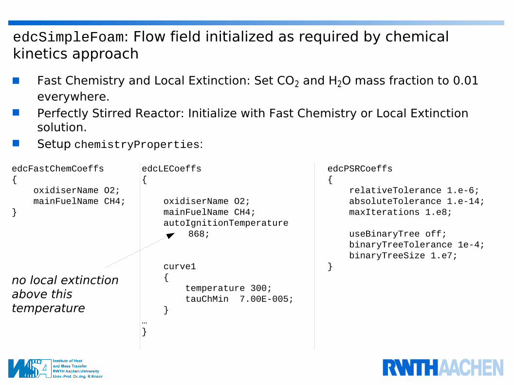
edcSimpleFoam: Flow field initialized as required by chemical kinetics approach
■ Fast Chemistry and Local Extinction: Set CO2 and H2O mass fraction to 0.01 everywhere.
■ Perfectly Stirred Reactor: Initialize with Fast Chemistry or Local Extinction solution.
■ Setup chemistryProperties:
edcFastChemCoeffs{ oxidiserName O2; mainFuelName CH4; }
edcPSRCoeffs{ relativeTolerance 1.e-6; absoluteTolerance 1.e-14; maxIterations 1.e8; useBinaryTree off; binaryTreeTolerance 1e-4; binaryTreeSize 1.e7; }
edcLECoeffs{
oxidiserName O2; mainFuelName CH4; autoIgnitionTemperature
868;
curve1 { temperature 300; tauChMin 7.00E-005; }…}
no local extinction above this temperature
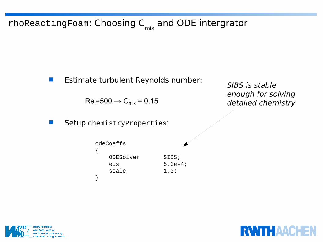
rhoReactingFoam: Choosing Cmix
and ODE intergrator
■ Estimate turbulent Reynolds number:
Ret=500 → Cmix = 0.15
■ Setup chemistryProperties:
odeCoeffs{ ODESolver SIBS; eps 5.0e-4; scale 1.0;}
SIBS is stable enough for solving detailed chemistry

Setting-up discretization schemes
■ Convective term: Linear upwind discretization (2nd order accurate)default Gauss linearUpwind cellLimited Gauss linear 1;
For species Yi (for rhoReactionFoam: Yi and hs)
div(phi,Yi) Gauss multivariateSelection
{
//hs linearUpwind cellLimited Gauss linear 1;
CH4 linearUpwind cellLimited Gauss linear 1;
O2 linearUpwind cellLimited Gauss linear 1;
…
}
■ Time discretization: (Pseudo) steady-state edcSimpleFoam (steady-state solver)
default steadyState;
rhoReactingFoam (transient solver)default SLTS phi rho 0.7;
default CoEuler phi rho 0.4;
global under-relaxation factor
max. CFL number
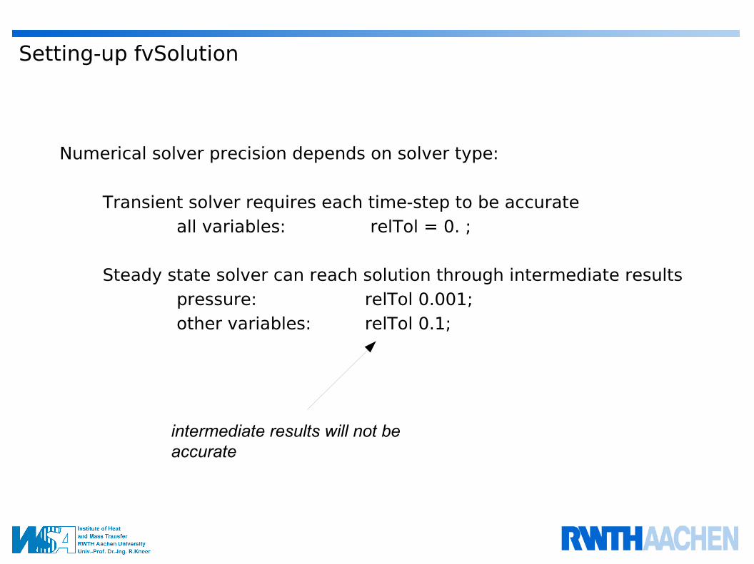
Setting-up fvSolution
Numerical solver precision depends on solver type:
Transient solver requires each time-step to be accurateall variables: relTol = 0. ;
Steady state solver can reach solution through intermediate resultspressure: relTol 0.001;other variables: relTol 0.1;
intermediate results will not be accurate
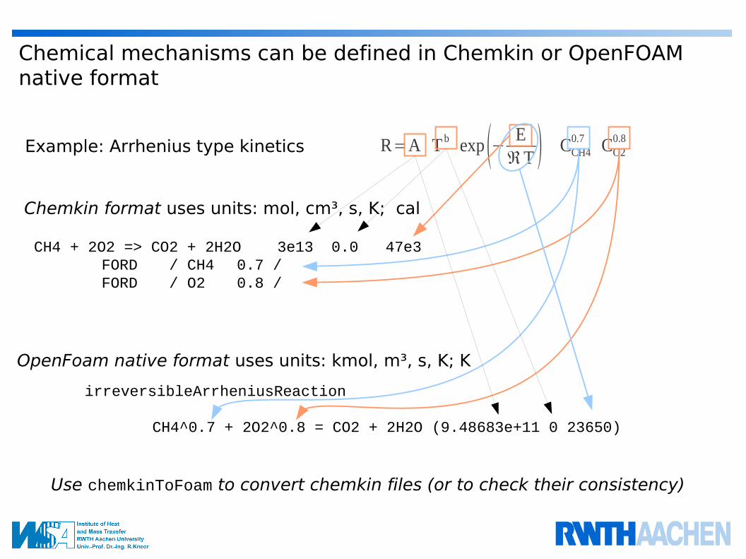
Chemical mechanisms can be defined in Chemkin or OpenFOAM native format
CH4 + 2O2 => CO2 + 2H2O 3e13 0.0 47e3FORD / CH4 0.7 /FORD / O2 0.8 /
Chemkin format uses units: mol, cm³, s, K; cal
Example: Arrhenius type kinetics
irreversibleArrheniusReaction
CH4^0.7 + 2O2^0.8 = CO2 + 2H2O (9.48683e+11 0 23650)
OpenFoam native format uses units: kmol, m³, s, K; K
Use chemkinToFoam to convert chemkin files (or to check their consistency)
R=A T b exp − EℜT CCH4
0.7 CO20.8
Overview
Theory
Tutorial case
Solution strategies
Validation

Combustion simulation often faces stability issues
Many error sources are possible because numerous models are applied simultaneously, for example:
■ Compressible flow■ Coupling of transport equations■ Numerically stiff reaction
mechanisms
Iterations
Residuals
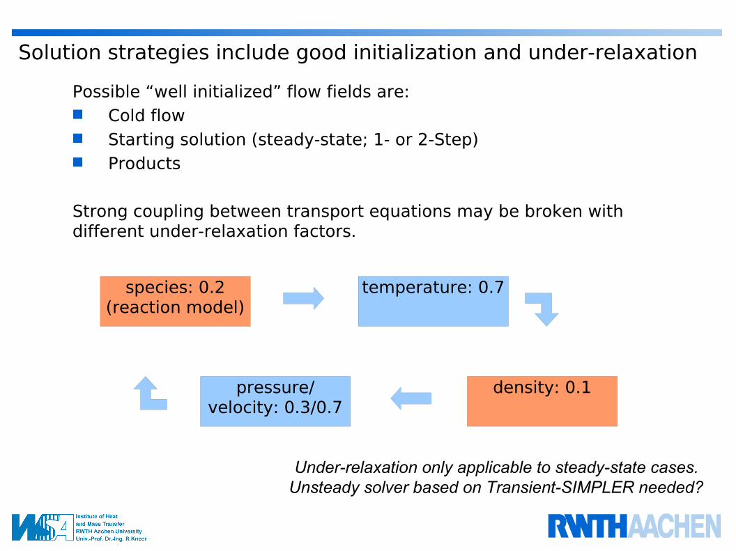
Solution strategies include good initialization and under-relaxation
Possible “well initialized” flow fields are:■ Cold flow■ Starting solution (steady-state; 1- or 2-Step)■ Products
Strong coupling between transport equations may be broken with different under-relaxation factors.
species: 0.2(reaction model)
temperature: 0.7
density: 0.1pressure/velocity: 0.3/0.7
Under-relaxation only applicable to steady-state cases. Unsteady solver based on Transient-SIMPLER needed?
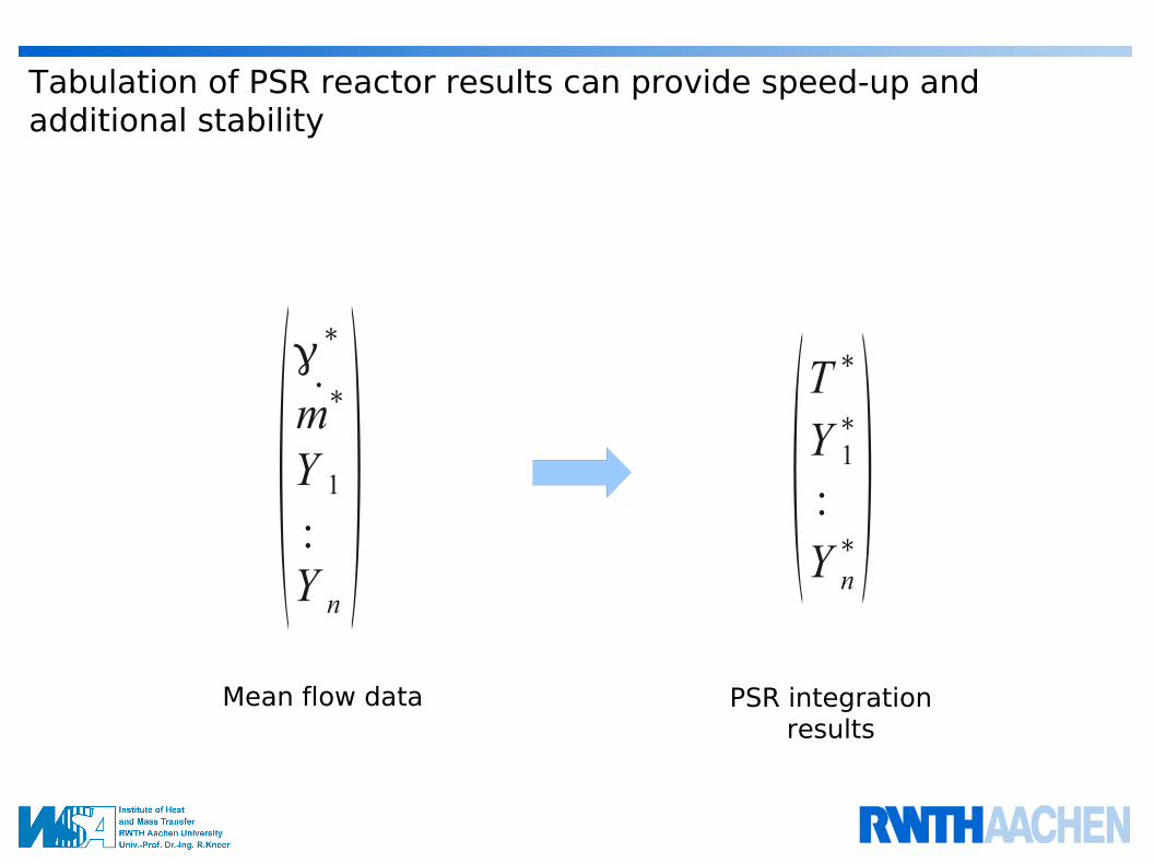
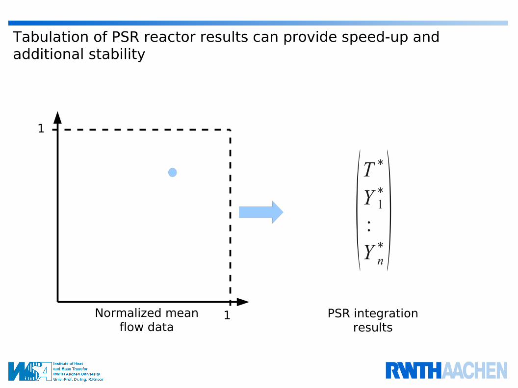
Tabulation of PSR reactor results can provide speed-up and additional stability
∗
m∗
Y 1:Y n
T∗
Y 1∗
:Y n
∗Mean flow data PSR integration
results
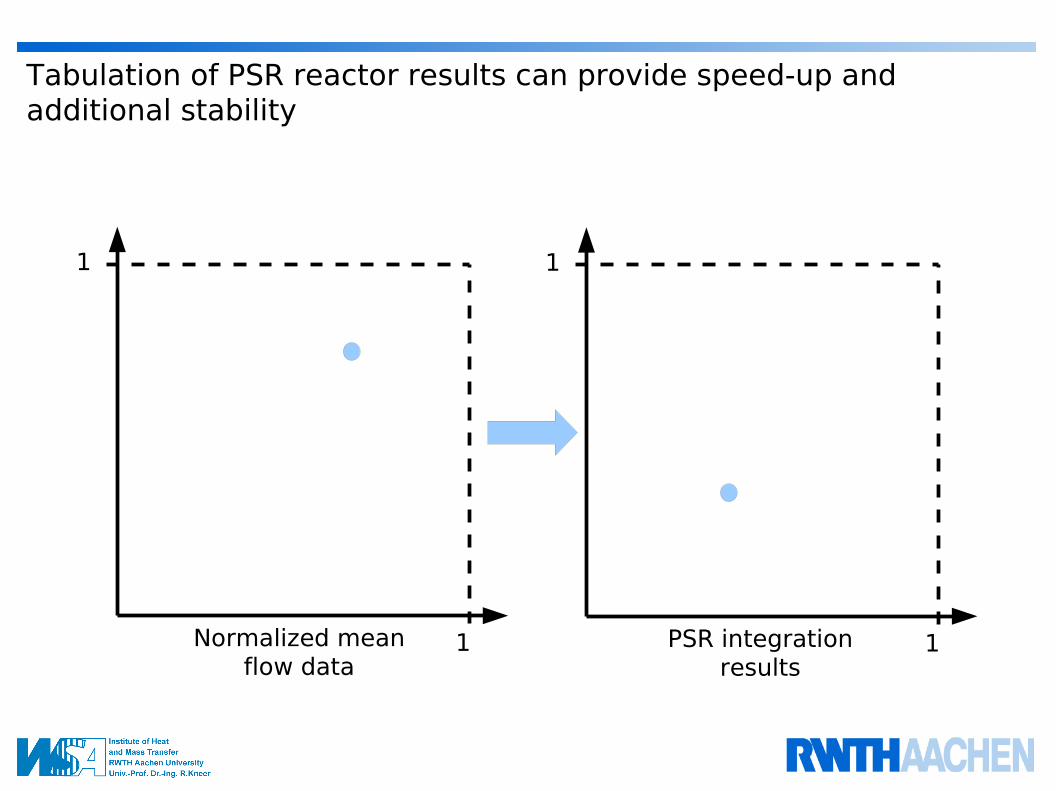
Tabulation of PSR reactor results can provide speed-up and additional stability
T∗
Y 1∗
:Y n
∗Normalized mean
flow dataPSR integration
results1
1
Tabulation of PSR reactor results can provide speed-up and additional stability
Normalized mean flow data
PSR integration results
1
1
1
1

1
1
1
1
Normalized mean flow data
PSR integration results
Tabulation of PSR reactor results can provide speed-up and additional stability
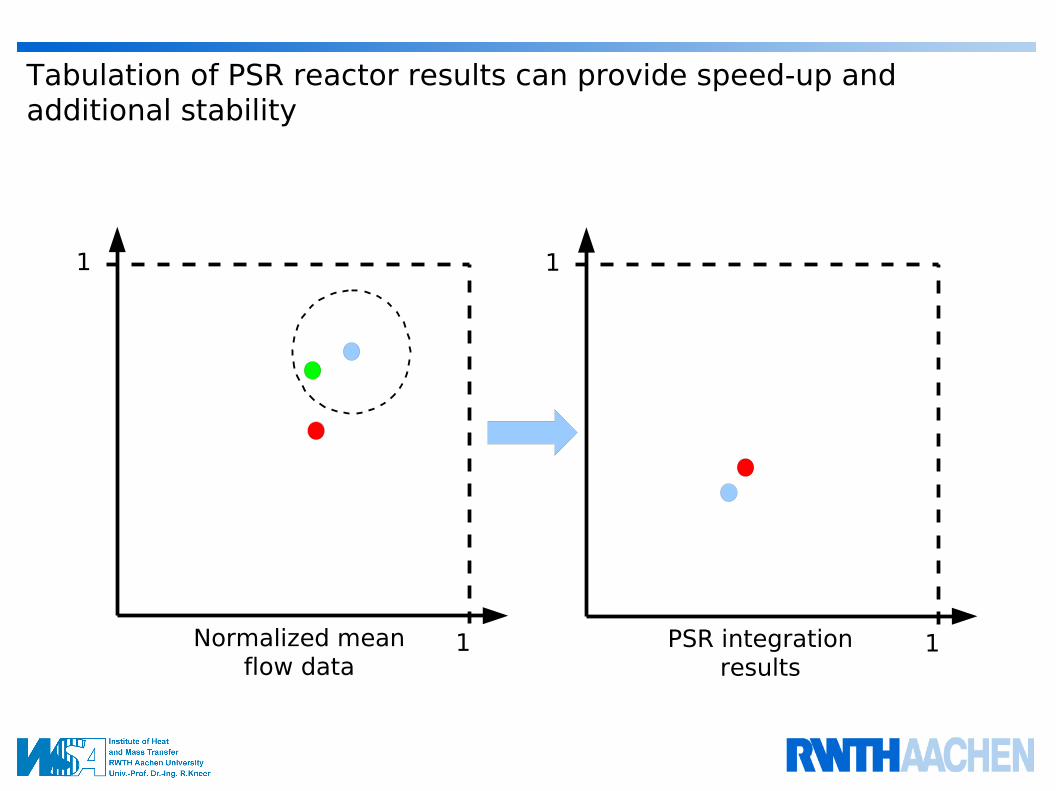
1
1
1
1
Normalized mean flow data
PSR integration results
Tabulation of PSR reactor results can provide speed-up and additional stability

1
1
1
1
Normalized mean flow data
PSR integration results
Tabulation of PSR reactor results can provide speed-up and additional stability
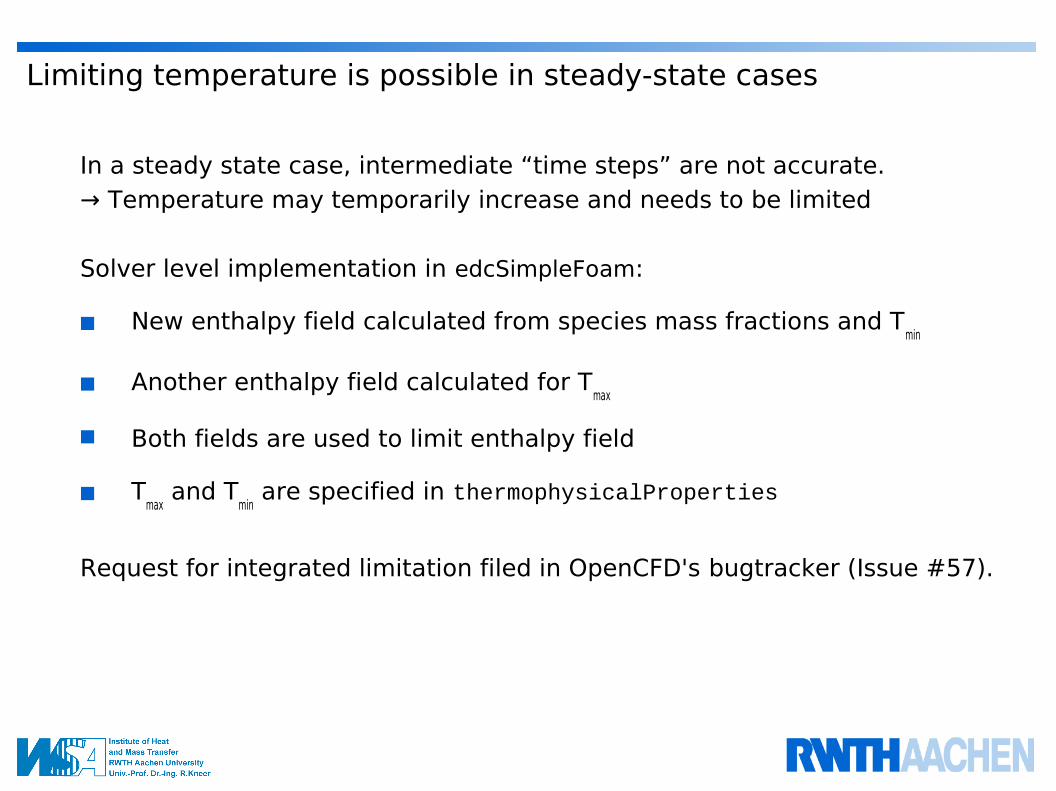
Limiting temperature is possible in steady-state cases
In a steady state case, intermediate “time steps” are not accurate. → Temperature may temporarily increase and needs to be limited
Solver level implementation in edcSimpleFoam:
■ New enthalpy field calculated from species mass fractions and Tmin
■ Another enthalpy field calculated for Tmax
■ Both fields are used to limit enthalpy field
■ Tmax
and Tmin are specified in thermophysicalProperties
Request for integrated limitation filed in OpenCFD's bugtracker (Issue #57).
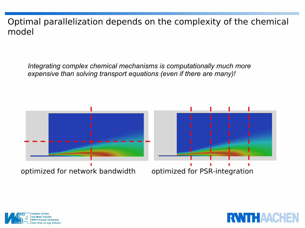
Optimal parallelization depends on the complexity of the chemical model
optimized for network bandwidth optimized for PSR-integration
Integrating complex chemical mechanisms is computationally much more expensive than solving transport equations (even if there are many)!
Overview
Theory
Tutorial case
Solution strategies
Validation

Detailed reaction mechnism predicts temperature profile accurately
Radiation modeling used with EDC, not used with PaSR.
Influence of Cmix is minimal
exp. data: Barlow, R. S. and Frank, J. H., Proc. Combust. Inst. 27:1087-1095 (1998)
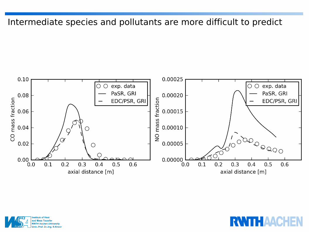
Intermediate species and pollutants are more difficult to predict
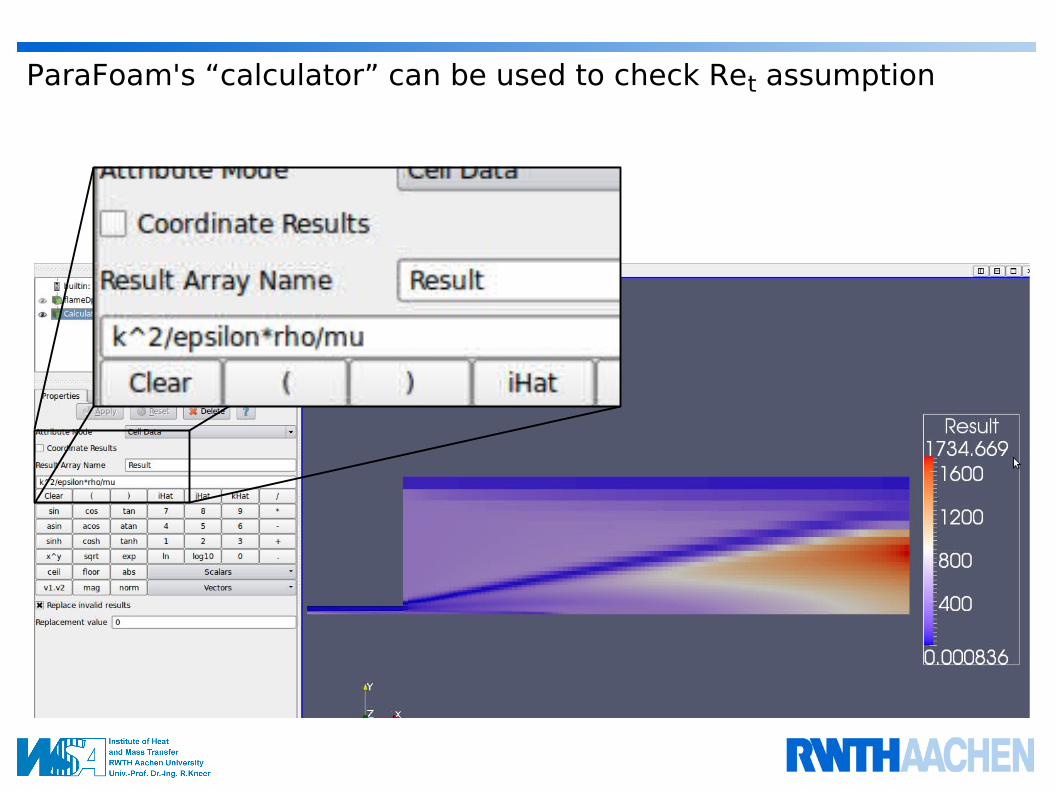
ParaFoam's “calculator” can be used to check Ret assumption
Comparison with measurements may require special post-processing
Common difficulties when comparing simulated mass fractions with measurements:
■ Measured data are often mole fractions or concentrationsIf not all (major) species are measured, correct conversion to mass fractions impossible
■ Flue gas or emission monitoring can be measured in “dry gas”, i.e. after water vapor has been condensed outSimulated data comprise a complete set, therefore they can be accurately converted
New utility massToMoleFraction handles conversion together with “-dryGas” option
for the EDC model:B. Magnussen: The Eddy Dissipation Concept: A Bridge between Science and Technology, ECCOMAS Thematic Conference on Computational Combustion, Lisbon, Portugal, 2005
for the validation of the OpenFoam implementation:B. Lilleberg, D. Christ, I.S. Ertesvåg, K.E. Rian, R. Kneer, Numerical simulation with an extinction database for use with the Eddy Dissipation Concept for turbulent combustion (submitted)
Final note: When using edcSimpleFoam or edcPisoFoam, please cite
Thank you for your attention!