Simulating seeded vacuum decay in a cold atom system
7
Simulating seeded vacuum decay in a cold atom system Thomas P. Billam, 1,* Ruth Gregory, 2,3,† Florent Michel, 2,‡ and Ian G. Moss 4,§ 1 Joint Quantum Centre (JQC) Durham-Newcastle, School of Mathematics, Statistics and Physics, Newcastle University, Newcastle upon Tyne, NE1 7RU, United Kingdom 2 Centre for Particle Theory, Durham University, South Road, Durham DH1 3LE, United Kingdom 3 Perimeter Institute, 31 Caroline Street North, Waterloo, Ontario N2L 2Y5, Canada 4 School of Mathematics, Statistics and Physics, Newcastle University, Newcastle upon Tyne NE1 7RU, United Kingdom (Received 30 November 2018; revised manuscript received 12 April 2019; published 23 September 2019) We propose to test the concept of seeded vacuum decay in cosmology using a Bose-Einstein condensate system. The role of the nucleation seed is played by a vortex within the condensate. We present two complementary theoretical analyses that demonstrate seeded decay is the dominant decay mechanism of the false vacuum. First, we adapt the standard instanton methods to the Gross-Pitaevskii equation. Second, we use the truncated Wigner method to study vacuum decay. DOI: 10.1103/PhysRevD.100.065016 I. INTRODUCTION First-order phase transitions form an important class of physical phenomena. Typically, these are characterized by metastable, supercooled states and the nucleation of bubbles. Applications range from the condensation of water vapor to the vacuum decay of fundamental quantum fields. In cosmology, bubbles of a new matter phase would produce huge density variations, and unsurprisingly first order phase transitions have been proposed as sources of gravitational waves [1,2] and as sources of primordial black holes [3,4]. Clearly a key factor in the relevance of such by-products of phase transitions is the likelihood of that transition occurring. Bubble nucleation rates are exponentially sup- pressed, and formal estimates of the lifetimes of metastable states can be huge. However, many phase transition rates in ordinary matter are greatly enhanced by the presence of nucleation seeds, in the form of impurities or defects on the boundary of the material. We have argued recently that cosmological bubble nucleation can also be greatly accel- erated by nucleation seeds, for example with seeds in the form of primordial black holes [5,6]. In this paper we propose that seeded bubble nucleation can be studied in a laboratory cold-atom analogue of cosmological vacuum decay [7,8]. The idea of using analogue systems for cosmological processes comes under the general area of modeling the “universe in the laboratory” [9,10]. So far, analogue systems have mostly been employed to test ideas in perturbative quantum field theory [11,12], but nonpertur- bative phenomena such as bubble nucleation also play an important role in quantum mechanics and field theory. As pointed out in the classic work of Coleman and others [13–15], the bubble nucleation process in quantum field theory can be described by an instanton, or bounce, solution to the field equations in imaginary time. The probability for decay is then given, to leading order, by a negative exponential of the action of the instanton. Understanding vacuum decay and the role of the instanton is now particularly pressing in light of the measurements of the Higgs mass, that currently indicates our vacuum is in a region of metastability [16]. The semiclassical description of vacuum decay with gravity involves analytically continuing to imaginary time, and finding the gravitational instanton. However, while most are comfortable with the assumptions used in pertur- bative quantum field theory on curved spacetime, such nonperturbative processes are sometimes viewed with more caution. The ability to test such a process via an analogue “table-top” quantum system would be a strong vindication of the use of such techniques. To this end, there have been some recent developments in exploring possible analogue systems that could test vacuum decay. Fialko et al. [7,8] proposed an experiment in a laboratory cold atom system. Their system consists of a Bose gas with two different spin states of the same atom species in an optical trap. The two * [email protected] † [email protected] ‡ [email protected] § [email protected] Published by the American Physical Society under the terms of the Creative Commons Attribution 4.0 International license. Further distribution of this work must maintain attribution to the author(s) and the published article’s title, journal citation, and DOI. Funded by SCOAP 3 . PHYSICAL REVIEW D 100, 065016 (2019) 2470-0010=2019=100(6)=065016(7) 065016-1 Published by the American Physical Society
Transcript of Simulating seeded vacuum decay in a cold atom system

Simulating seeded vacuum decay in a cold atom system
Thomas P Billam1 Ruth Gregory23dagger Florent Michel2Dagger and Ian G Moss4sect1Joint Quantum Centre (JQC) Durham-Newcastle School of Mathematics Statistics and Physics
Newcastle University Newcastle upon Tyne NE1 7RU United Kingdom2Centre for Particle Theory Durham University South Road Durham DH1 3LE United Kingdom
3Perimeter Institute 31 Caroline Street North Waterloo Ontario N2L 2Y5 Canada4School of Mathematics Statistics and Physics Newcastle University
Newcastle upon Tyne NE1 7RU United Kingdom
(Received 30 November 2018 revised manuscript received 12 April 2019 published 23 September 2019)
We propose to test the concept of seeded vacuum decay in cosmology using a Bose-Einstein condensatesystem The role of the nucleation seed is played by a vortex within the condensate We present twocomplementary theoretical analyses that demonstrate seeded decay is the dominant decay mechanism ofthe false vacuum First we adapt the standard instanton methods to the Gross-Pitaevskii equation Secondwe use the truncated Wigner method to study vacuum decay
DOI 101103PhysRevD100065016
I INTRODUCTION
First-order phase transitions form an important class ofphysical phenomena Typically these are characterizedby metastable supercooled states and the nucleation ofbubbles Applications range from the condensation of watervapor to the vacuum decay of fundamental quantum fieldsIn cosmology bubbles of a new matter phase wouldproduce huge density variations and unsurprisingly firstorder phase transitions have been proposed as sourcesof gravitational waves [12] and as sources of primordialblack holes [34]Clearly a key factor in the relevance of such by-products
of phase transitions is the likelihood of that transitionoccurring Bubble nucleation rates are exponentially sup-pressed and formal estimates of the lifetimes of metastablestates can be huge However many phase transition rates inordinary matter are greatly enhanced by the presence ofnucleation seeds in the form of impurities or defects on theboundary of the material We have argued recently thatcosmological bubble nucleation can also be greatly accel-erated by nucleation seeds for example with seeds in theform of primordial black holes [56] In this paper wepropose that seeded bubble nucleation can be studied in a
laboratory cold-atom analogue of cosmological vacuumdecay [78]The idea of using analogue systems for cosmological
processes comes under the general area of modeling theldquouniverse in the laboratoryrdquo [910] So far analoguesystems have mostly been employed to test ideas inperturbative quantum field theory [1112] but nonpertur-bative phenomena such as bubble nucleation also play animportant role in quantum mechanics and field theoryAs pointed out in the classic work of Coleman and others
[13ndash15] the bubble nucleation process in quantum fieldtheory can be described by an instanton or bouncesolution to the field equations in imaginary time Theprobability for decay is then given to leading order by anegative exponential of the action of the instantonUnderstanding vacuum decay and the role of the instantonis now particularly pressing in light of the measurementsof the Higgs mass that currently indicates our vacuum is ina region of metastability [16]The semiclassical description of vacuum decay with
gravity involves analytically continuing to imaginary timeand finding the gravitational instanton However whilemost are comfortable with the assumptions used in pertur-bative quantum field theory on curved spacetime suchnonperturbative processes are sometimes viewed with morecaution The ability to test such a process via an analogueldquotable-toprdquo quantum system would be a strong vindicationof the use of such techniques To this end there have beensome recent developments in exploring possible analoguesystems that could test vacuum decay Fialko et al [78]proposed an experiment in a laboratory cold atom systemTheir system consists of a Bose gas with two different spinstates of the same atom species in an optical trap The two
thomasbillamnclacukdaggerrawgregorydurhamacukDaggerflorentcmicheldurhamacuksectianmossnclacuk
Published by the American Physical Society under the terms ofthe Creative Commons Attribution 40 International licenseFurther distribution of this work must maintain attribution tothe author(s) and the published articlersquos title journal citationand DOI Funded by SCOAP3
PHYSICAL REVIEW D 100 065016 (2019)
2470-0010=2019=100(6)=065016(7) 065016-1 Published by the American Physical Society
states are coupled by a microwave field By modulating theamplitude of the microwave field a new quartic interactionbetween the two states is induced in the time-averagedtheory which creates a nontrivial ground state structure asillustrated in Fig 1 [17]In this paper we propose an analogue system that can
explore the process of catalysis of vacuum decay that iscentral to our previous results We use the above model totest seeded vacuum decay by introducing a vortex intothe two dimensional spinor Bose gas system We have usedtwo complementary theoretical approaches First we haveapplied Colemanrsquos non-perturbative theory of vacuumdecay to the Gross-Pitaevskii equation (GPE) Secondwe have used the truncated Wigner method a stochasticapproach to study the vacuum decay In both cases we findthat the introduction of the vortex seed enhances theprobability of vacuum decay
II SYSTEM
Our system is a two-component BEC of atoms withmass m coupled by a modulated microwave field TheHamiltonian operator in n dimensions is given by
H frac14Z
dnx
ψdaggeri
minusℏ2nabla2
2m
ψ i thorn Vethψ iψ
daggeri THORN eth1THORN
with field operators ψ i i frac14 1 2 and summation over thespin indices implied Fialko et al [78] described aprocedure whereby averaging over timescales longer thanthe modulation timescale leads to an interaction potentialof the form
Vfrac14 g2ethψdagger
i THORN2ethψ iTHORN2minusμψdaggeriψ iminusνψdagger
i σxijψ jthorngνλ2
4μethψdagger
i σyijψ jTHORN2
eth2THORN
where the σi are the Pauli matrices The potentialincludes the chemical potential μ intracomponent s-wave
interactions of strength g between the field operators (weassume intercomponent s-wave interactions are negligible)and the microwave induced interaction ν The final termcomes from the averaging procedure and introduces anew parameter λ dependent on the amplitude of themodulation The trapping potential used to confine thecondensate has been omitted in order to isolate the physicsof vacuum decayThe terms proportional to ν are responsible for the
difference in energy between the global and local minimaof the energy The global minimum represents the truevacuum state and the local minimum represents the falsevacuum In order to parametrize the difference in energybetween the vacua we introduce a ldquosmallrdquo dimensionlessparameter ϵ by
ϵ frac14ν
μ
1=2
eth3THORN
For ν gt 0 the true vacuum is a state with ψ1 frac14 ψ2 and thefalse vacuum is a state with ψ1 frac14 minusψ2 The condensatedensities of the two components at the extrema are equal toone another and given by hψdagger
1ψ1i frac14 hψdagger2ψ2i frac14 ρmeth1 ϵ2THORN
Note that we prefer to work with the mean density ρm frac14μ=g rather than the chemical potential The difference inenergy density between the two vacuum states is givenby ΔV frac14 4gρ2mϵ2
III INSTANTON TREATMENT
The nonperturbative theory of vacuum decay starts withthe imaginary-time partition function
Z frac14Z
Dψ iDψ ieminusSfrac12ψ iψ i=ℏ eth4THORN
where the integral extends over complex fields ψ i and theircomplex conjugates ψ i with action
Sfrac12ψ iψ ifrac14Z
dnxdτ
ℏψ ipartτψ iminus ψ i
ℏ2
2mnabla2ψ ithornVethψ iψ iTHORN
eth5THORN
Vacuum decay is associated with instanton solutions tofield equations in imaginary time τ frac14 it [1314]
ℏ2
2mnabla2ψ i minus ℏpartτψ i minus
partVpartψ i
frac14 0
ℏ2
2mnabla2ψ i thorn ℏpartτψ i minus
partVpartψ i
frac14 0 eth6THORN
and fields that approach the false vacuum as r τ rarr infinOn the original path integration contour ψ i and ψ i are
complex conjugates and the field equations imply that thesaddle points are static In order to find the nonstatic bubble
FIG 1 The field potential V plotted as a function of the relativephase of the two atomic wave functions φ The false vacuum isthe minimum at φ frac14 π and the true vacuum the global minimumat φ frac14 0 ΔV is the difference in vacuum energy
BILLAM GREGORY MICHEL and MOSS PHYS REV D 100 065016 (2019)
065016-2
solutions we have to deform the path of integration into awider region of complex function space where ψ i is not thecomplex conjugate of ψ i Although this may appear astrange procedure at first sight this analytic continuation isalready implicit in the previous work on vacuum decay aswe shall see laterThe full expression for the nucleation rate of vacuum
bubbles in a volume V is [1314]
Γ asymp V
det0S00frac12ψb
det S00frac12ψ fvminus1=2
Sfrac12ψb2πℏ
N=2
eminusSfrac12ψb=ℏ eth7THORN
where S00 denotes the second functional derivative of theaction S and det0 denotes omission of N frac14 nthorn 1 zeromodes from the functional determinant of the operator(For convenience we always include a constant shift to theaction so that the action of the false vacuum is zero) Forseeded nucleation the volume factor is replaced by thenumber of nucleation seeds and the number of zero modesbecomes N frac14 1 The key feature here is the exponentialsuppression of the decay rate and the nonperturbativetreatment fails if the exponent is smallIn vacuum decay the key quantity determining physical
aspects of decay is the energy splitting between true andfalse vacua ΔV which is proportional to ϵ2 In our systemϵ also determines the magnitude of the interaction betweenthe two scalars and for small ϵ most of the degrees offreedom of the system decouple leaving an effective fieldtheory of the relative phases of the two condensates asexplored in [78] in one spatial dimensionHere we are interested in seeded decay so we consider
the model in two spatial dimensions with polar coordinatesr and θ The natural size of the bubble will be determinedby R0 frac14 ℏethρm=mΔVTHORN1=2 and the natural timescale byR0=cs where the sound speed cs frac14 ethgρm=mTHORN1=2 To sim-plify the following analysis we rescale our dimensionfulcoordinates accordingly and also rescale the action
S frac14 ℏρmR20S eth8THORN
Since we are interested in exploring seeded decay welook for a cylindrically symmetric solution that explicitlyhighlights the relevant degrees of freedommdashnamely therelative phase φethr τTHORN between the two components theleading order (in ϵ) profile of the false vacuum backgroundρethr τTHORN an overall common phase winding nθ that is presentin a nontrivial vortex background and the bubble profilefunction σethr τTHORNmdashand includes the possibility of a topo-logically nontrivial vortex false vacuum state
ψ i frac14 ρ1=21 ϵ
2σ
eiφ=2thorninθ
ψ i frac14 ρ1=21 ϵ
2σ
e∓iφ=2minusinθ eth9THORN
where we adopt the convention that the upperlower signsapply to the i frac14 1 2 spin states respectivelyThe pure false vacuum has n frac14 0 and ρ frac14 ρmeth1 minus ϵ2THORN
with instanton profiles for φ explored in [78] Here we areinterested in seeded tunneling so we also consider thevortex background for n frac14 1 with ρ satisfying the Oethϵ2THORNbackground equations obtained by substituting (9) in (6)The profile of ρ is precisely that of a superfluid (or global)vortex and is illustrated in Fig 2The potential for the instanton solutions depends only
on the relative phase φ and the background density ρOur rescaling of the length and time coordinates means thatwe also rescale the potential to V frac14 2ethV minus VTVTHORN=ΔV
V frac14 ρeth1 minus cosφTHORN thorn 1
2λ2ρ2sin2φ eth10THORN
as plotted in Fig 1 At zeroth order in ϵ the fieldequations (6) imply that σ frac14 minusiρminus1partτφ Note that σ isimaginary and the bubble solution has ψ1 ne ψdagger
1 as wasmentioned earlier Replacing σ in the action using this fieldequation gives a Klein-Gordon type action depending onlyon φ which was used in Refs [78]
Sfrac12φ frac14 ϵ
Zdnxdτ
1
2ρethnablaφTHORN2 thorn 1
2_φ2 thorn V
eth11THORN
However at the core of the vortex ρ rarr 0 and thisreplacement of σ is no longer valid Instead numericalsolutions have been obtained by solving the full equationsfor the phase φ and the density variation σThe vacuum decay rate around a single vortex using
Colemanrsquos formula (7) with a single zero mode is
Γ frac14 AcsR0
ρmR2
0S2π
1=2
eminusρmR20S eth12THORN
where A is a dimensionless numerical factor depending onthe ratio of determinants (which we do not evaluate here)
00 25 50 75 100 125 150r ( R0)
000
025
050
075
100
(1minus
2 )
FIG 2 Vortex density profile ρ frac14 ρ=ρm plotted as a functionof radius r The density vanishes at the center and approachesthe false vacuum density as r rarr infin Its physical thicknessscales as ϵR0
SIMULATING SEEDED VACUUM DECAY hellip PHYS REV D 100 065016 (2019)
065016-3
Numerical results for the factor S in the decay exponentare shown in Fig 3 [20] These show clearly that thetunneling exponent can be reduced significantly in thepresence of a vortex The vortex width from Fig 2 is relatedto ϵR0 Consequently smaller values of ϵ are associatedwith relatively thin vortices compared to the bubble scaleR0 which have less effect on the vacuum decay rate thanvortices with larger values of ϵThe nucleation rate depends on the physical parameters
through the combination ρmR20 The length scale R0 itself
is related to the atomic scattering length as and thethickness of the condensate az via the effective couplingstrength g [22]
g frac14 4πℏ2
masffiffiffiffiffiffi2π
paz
eth13THORN
Thus the factor in the decay exponent becomes ρmR20 frac14
az=eth4ϵ2ffiffiffiffiffiffi8π
pasTHORN
IV STOCHASTIC TREATMENT
A Overview
As an alternative treatment of bubble nucleation wemodel a two-dimensional spinor BEC using a truncatedWigner approach At the mean-field level the system canbe described by the Gross-Pitaevskii equation (GPE)derived from the symmetric Hamiltonian in the rescaledcoordinates used above
iparttψ i frac14 minusϵnabla2ψ i thorn ϵVTψ i thorn ϵρmpartVpartψ i
eth14THORN
where
partVpartψ i
frac14 1
2ϵ2
ψ iψ i
ρmminus 1
ψ i
ρmminus1
2
ethσxψTHORNiρm
thorn λ2
4
ψσyψ
ρm
ethσyψTHORNiρm
eth15THORN
Here VT is the dimensionless form of an optical trappingpotential that affects both spin states equally The dimen-sional trapping potential is VT frac14 2gρmϵ2VT The truncatedWigner approach seeks to emulate the many-body quantumfield description of a BEC with a stochastic description[2324] At zero temperature it consists of seeding appro-priate modes of the system with an average of 1=2 particleper mode of stochastic noise in the initial conditions andthen evolving in time with the GPE The stochastic noiseemulates vacuum fluctuationsWe add stochastic noise to an ensemble of initial fields
and compute the trajectory of each field using the projectedGPE (PGPE) to precisely evolve the noise-seeded modes[24] including a correction to the nonlinear term to accountfor the average noise density [8] In a periodic 2D squarebox of side length L this corresponds to propagating theequation
iparttψ i frac14 P
minusϵnabla2 thorn ϵVT thornjψ ij2 minus M
L2
2ϵρmminus
1
2ϵ
ψ i
thornminusϵ
2thorn ϵλ2
4ρmethψ iψ
3minusi minus ψ
iψ3minusiTHORNψ3minusi
eth16THORN
where the projection operator P restricts the field to the Mlowest-energy plane wave modes
B Vortex-seeded decay in an infinite system
Taking a periodic 2D square box of side length L webegin with the false vacuum solution to the GPE
ψ iFV frac14 ρ1=2m eth1 minus ϵ2THORN1=2eiπ=2 eth17THORNWe evolve the PGPE (16) using a Fourier pseudospectralmethod implemented using XMDS2 software [25] with Pgrid points in each direction The projector P restrictsthe field to the M modes satisfying jkj lt πP=eth2LTHORN Thuswe create an initial ensemble of fields by adding noise intothese M plane-wave modes
ψ i frac14 ψ iFV thorn 1
LPX
k
βikeikmiddotr eth18THORN
where βik are complex Gaussian random variables withhβikβjk0 i frac14 δijδkk0=2 To determine a decay rate withoutvortices we evolve trajectories directly from this initialensembleTo investigate the effects of vortices on the decay rate
we take an initial ensemble as described above but prior toevolving trajectories we imprint the density and phaseprofiles of vortices into the system Since our periodic box
12
10
8
6
4
2
0005 010 015 020 025
FIG 3 The dimensionless exponent S of the vacuum decay rateplotted as a function of the parameter ϵ2 The solid lines representunseeded vacuum decay and the dashed lines are for bubblesseeded by vortices The action is lower for the seeded bubbles
BILLAM GREGORY MICHEL and MOSS PHYS REV D 100 065016 (2019)
065016-4
requires a net-neutral distribution of vortices we use thetechniques described in Ref [26] to imprint a square gridpattern comprising two clockwise-circulating and twoanticlockwise-circulating vortices The vorticesrsquo mutualx and y separations are set to L=2 and diagonally opposedvortices have the same circulationIn Fig 4 we show typical examples of the stochastic
trajectories with and without the imprinted vortices [Theseare frames from the movies included as SupplementalMaterial [27]] We observe bubbles of true vacuum tonucleate most often at the locations of the vortices whenthey are present although nucleation in the bulk doesremain possible in the presence of vortices To quantita-tively investigate the increase in the rate of nucleation weevolve an ensemble of 1000 trajectories both with andwithout vortices As in Ref [8] we evaluate the averagevalue of cosϕ across all simulation grid points in eachtrajectory and consider a trajectory to have nucleated a
bubble of true vacuum when this average exceeds minus095In Fig 5 we plot the fraction of trajectories that have failedto nucleate a bubble as a function of time FethtTHORN Wedetermine approximate decay rates by least-squares fittingan exponential decay to FethtTHORN over the time interval where itbest resembles an exponential decay (determined by eyefrom Fig 5) Taking λ frac14 115 we find Γ asymp eth29 01THORN times10minus3cs=R0 without vortices and Γasympeth262THORNtimes10minus3cs=R0
with vortices For λ frac14 12 we find Γ asymp eth19 02THORN times10minus5cs=R0 without vortices and Γ asymp eth700 20THORN times10minus5cs=R0 with vortices The quoted uncertainties estimatethe statistical uncertainty in the stochastic method by abootstrap calculation [28] Clearly the presence of vorticesgreatly enhances the rate of vacuum decay in this system
C Vortex-seeded decay in a trapped system
To investigate the potential for realizing these results inexperiments we repeat our stochastic simulations for thecase of a spinor BEC contained inside a circular opticalldquobucketrdquo trap of radius R
VTethrTHORN frac14V0
2
1thorn tanh
r minus Rw
eth19THORN
where V0 is the (dimensionless) trap depth and w para-metrizes the wall-steepness of the trap We apply thetruncated Wigner formalism as described above but mak-ing an approximation for the initial stochastic noise
ψ i frac14 ψ iFV thorn fethrTHORNL
PX
k
βikeikmiddotr
eth20THORN
minus20
0
20 (a) (d)
minus20
0
20 (b) (e)
minus 20 0 20
minus20
0
20 (c)
minus 20 0 20
(f)
minus 1
0
1
x (R0)
y(R
0)
cos
FIG 4 Typical examples of the decay of the false vacuum withand without imprinted vortices in a two-dimensional periodicsystem The plots show the cosine of the relative phase betweenthe two spin states Dimensionless parameters are λ frac14 115ϵ frac14 0316 ρmR2
0 frac14 600 and L frac14 4267R0 Our numerical gridhas P frac14 128 (a) Initially the false vacuum predominates (b) Astime progresses bubbles of true vacuum (yellow) nucleatepredominantly around the vortices (c) Later still nucleatedbubbles expand to fill the system (dndashf) Typical trajectorieswithout imprinted vortices [same times as (andashc)] illustrate thenucleation of bubbles at random locations which occurs at aslower rate than vortex-seeded nucleation
0 500 1000 1500t (R0 cs)
minus4
minus3
minus2
minus1
0
1
log[
F(t
)]
= 115
= 12
0 10 4minus02
minus01
00
FIG 5 Fraction of trajectories failing to nucleate a bubble oftrue vacuum by a given time FethtTHORN both with and without vortices(dashed and solid lines respectively) The straight grey lines showexponential decays fitted over selected regions
SIMULATING SEEDED VACUUM DECAY hellip PHYS REV D 100 065016 (2019)
065016-5
where the function fethrTHORN frac14 ΘethR minus rTHORN restricts the noise tothe trap interior We then evolve the PGPE as describedabove both with and without initial imprinting of thedensity and phase profiles of a vortex at the trap centerNumerical results shown in Fig 6 confirm that the
vortex continues to act as nucleation seed in this systemholding out the possibility of experimental observation ofthis effect However we also observe that the walls of thetrap strongly enhance bubble nucleation both with andwithout the imprinted vortex Our numerics show that therate of vortex seeding at the trap walls is dependent on thewall steepness w with steeper walls reducing the rateThis is a boundary effect due to the fact that the densityoutside of the trap is low allowing the phase to fluctuatewidely as seen in the first frame of Fig 6 This could be
interpreted as the exterior of the trap being full of ldquoghostrdquo
vortices that then migrate to the wall and trigger bubblenucleation and may be of interest for laboratory BECsHowever in an unbounded system such as our universethis boundary effect is irrelevant and the only possibleseed will be the vortex
V CONCLUSION
In conclusion our two theoretical approaches based onthe Euclidean field equations (6) and on the truncatedWigner approximation both show a significant increase ofthe decay rate of the false vacuum in the presence of avortex in agreement with our previous work on cosmo-logical phase transitions Both the quantum calculation andthe TW approach agree on this conclusion although theTW approach gives faster vacuum decay in all cases thanthe quantum calculation does We believe this is likely to bedue to the energy content of the stochastic fluctuationswhich gives a boost to crossing the potential barrier It maybe possible to account for this effect by renormalizing theparameters of the potential in the TWapproach We plan toinvestigate this further and conduct a thorough comparisonof the different approaches in a simpler 1D systemNumerical simulations also indicate that other kinds of
defects such as the walls of a sharp potential trap canalso enhance decay Since getting a large enough decayrate is a major difficulty in designing experiments weexpect this to be an important ingredient for putting thetheoretical model of [78] into practice and thus testingvacuum decay in the laboratory While our simulationsrepresent a proof-of-principle example rather than aconcrete experimental proposal advances in opticaltrapping [2930] and various techniques for vorteximprinting in spinor condensates [3132] could be usedto probe similar systems experimentallyData supporting this publication is openly available
under a Creative Commons CC-BY-40 License [33]
ACKNOWLEDGMENTS
We would like to thank Carlo Barenghi for helpfulsuggestions This work was supported in part by theLeverhulme Trust [Grant No RPG-2016-233] theEngineering and Physical Sciences Research Council(Grant No EPR0210741) and by the PerimeterInstitute Research at Perimeter Institute is supported bythe Government of Canada through the Department ofInnovation Science and Economic Development and bythe Province of Ontario through the Ministry of Researchand Innovation R G would also like to thank the SimonsFoundation for support and the Aspen Center for Physics forhospitality F M thanks Fundaccedilatildeo de Amparo a` Pesquisado Estado de Satildeo Paulo for support This research made useof the Rocket High Performance Computing service atNewcastle University
minus50
0
50(a) (d)
minus50
0
50(b) (e)
minus 50 0 50
minus50
0
50(c)
minus 50 0 50
(f)
minus1
0
1
x (R0)
y(R
0)
cos
FIG 6 Examples of the decay of the false vacuum with andwithout an imprinted vortex in a two-dimensional ldquobucketrdquo trapThe plots show the cosine of the relative phase between the twospin states Dimensionless parameters are λ frac14 115 ϵ frac14 0316ρmR2
0 frac14 320 and L frac14 17068R0 Our numerical grid hasP frac14 512 The BEC is contained inside a circular bucket trapVTethrTHORN frac14 V0f1thorn tanhfrac12ethr minus RTHORN=wg=2 parametrized by strengthV0 frac14 100 radius R frac14 64R0 and wall steepness w frac14 2R0 (a) Ini-tially the false vacuum predominates within the circular trap butbubbles of true vacuum rapidly form around the walls of the trap(b) Later a bubble of true vacuum (yellow) forms around thevortex in the center (c) Later still the true vacuum regions growand eventually merge (dndashf) Typical trajectory without an initiallyimprinted vortex [same times as (andashc)]
BILLAM GREGORY MICHEL and MOSS PHYS REV D 100 065016 (2019)
065016-6
[1] C Caprini R Durrer T Konstandin and G Servant PhysRev D 79 083519 (2009)
[2] M Hindmarsh S J Huber K Rummukainen and D JWeir Phys Rev Lett 112 041301 (2014)
[3] S W Hawking I G Moss and J M Stewart Phys Rev D26 2681 (1982)
[4] H Deng and A Vilenkin J Cosmol Astropart Phys 12(2017) 044
[5] R Gregory I Moss and B Withers J High Energy Phys03 (2014) 081
[6] P Burda R Gregory and I Moss Phys Rev Lett 115071303 (2015)
[7] O Fialko B Opanchuk A I Sidorov P D Drummondand J Brand Europhys Lett 110 56001 (2015)
[8] O Fialko B Opanchuk A I Sidorov P D Drummondand J Brand J Phys B At Mol Opt Phys 50 024003(2017)
[9] T Roger C Maitland K Wilson N Westerberg D VockeE M Wright and D Faccio Nat Commun 7 13492(2016)
[10] S Eckel A Kumar T Jacobson I B Spielman and G KCampbell Phys Rev X 8 021021 (2018)
[11] W G Unruh Phys Rev Lett 46 1351 (1981)[12] C Barcelo S Liberati and M Visser Living Rev
Relativity 8 12 (2005) 14 3 (2011)[13] S R Coleman Phys Rev D 15 2929 (1977) 16 1248(E)
(1977)[14] C G Callan and S R Coleman Phys Rev D 16 1762
(1977)[15] S R Coleman and F De Luccia Phys Rev D 21 3305
(1980)[16] G Degrassi S Di Vita J Elias-Miro J R Espinosa G F
Giudice G Isidori and A Strumia J High Energy Phys 08(2012) 098
[17] It has been pointed out that there is an instability in theequations describing the modulated system [1819] How-ever for the parameters used in this paper and trap radius25 μm with 39K the instability occurs for a modulationfrequency ω lt 800k2 Hz where k is the maximum wavenumber consistent with the equations in units of the healinglength We will assume that the modulation frequency isabove this limit
[18] J Braden M C Johnson H V Peiris A Pontzen and SWeinfurtner Phys Rev Lett 123 031601 (2019)
[19] J Braden M C Johnson H V Peiris and S WeinfurtnerJ High Energy Phys 07 (2018) 014
[20] We have checked these results using an ansatz approachakin to that of [21] extended to include dispersion Theresults agree within a few per cent
[21] B-H Lee W Lee R MacKenzie M B Paranjape U AYajnik and D-h Yeom Phys Rev D 88 085031 (2013)
[22] M D Lee S A Morgan M J Davis and K Burnett PhysRev A 65 043617 (2002)
[23] S Chaturvedi and P D Drummond Eur Phys J B 8 251(1999)
[24] P Blakie A Bradley M Davis R Ballagh and CGardiner Adv Phys 57 363 (2008)
[25] G R Dennis J J Hope and M T Johnsson ComputPhys Commun 184 201 (2013)
[26] T P Billam M T Reeves B P Anderson and A SBradley Phys Rev Lett 112 145301 (2014)
[27] See Supplemental Material at httplinkapsorgsupplemental101103PhysRevD100065016 for moviesshowing examples of the dynamics
[28] We estimate the uncertainties in the rate by a two-stepbootstrap procedure First we create 250 sample datasets (of1000 trajectories each) by randomly choosing trajectoriesfrom our actual dataset of 1000 trajectories with replace-ment Secondly we fit an exponential decay to each sampledataset using least-squares fitting as described above Thequoted error is the standard deviation of the distribution of250 rates obtained from fitting these sample datasets Theuncertainty obtained by this simple estimate is orders ofmagnitude larger that the least-squares fitting error of asingle dataset suggesting the latter is not a realistic estimateof the overall uncertainty
[29] A L Gaunt T F Schmidutz I Gotlibovych R P Smithand Z Hadzibabic Phys Rev Lett 110 200406 (2013)
[30] G Gauthier I Lenton N M Parry M Baker M J DavisH Rubinsztein-Dunlop and TW Neely Optica 3 1136(2016)
[31] Y Kawaguchi and M Ueda Phys Rep 520 253 (2012)[32] D M Stamper-Kurn and M Ueda Rev Mod Phys 85
1191 (2013)[33] T P Billam R Gregory F Michel and I G Moss Data
supporting publication Simulating seeded vacuum decay ina cold atom system httpsdoiorg1025405datancl9639143
SIMULATING SEEDED VACUUM DECAY hellip PHYS REV D 100 065016 (2019)
065016-7
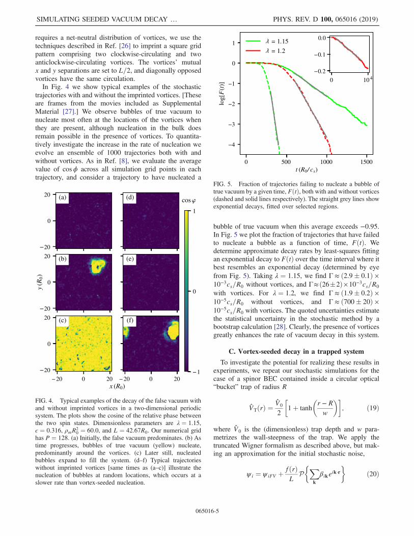