Simplified Numerical Model for the Study of Wave Energy Convertes (WECs)€¦ · Introduction...
55
Introduction Aproximation Identification Applications Simplified Numerical Model for the Study of Wave Energy Convertes (WECs) J. A. Armesto, R. Guanche, A. Iturrioz and A. D. de Andres Ocean Energy and Engineering Group “IH Cantabria”, Universidad de Cantabria October 18 th , 2013 Armesto, Guanche, Iturrioz and de Andres 18/X/2012 Simplified Numerical Model for WECs
Transcript of Simplified Numerical Model for the Study of Wave Energy Convertes (WECs)€¦ · Introduction...
Introduction Aproximation Identification Applications
Simplified Numerical Model for the Study of WaveEnergy Convertes (WECs)
J. A. Armesto, R. Guanche, A. Iturrioz and A. D. de Andres
Ocean Energy and Engineering Group“IH Cantabria”, Universidad de Cantabria
October 18th, 2013
Armesto, Guanche, Iturrioz and de Andres 18/X/2012 Simplified Numerical Model for WECs

Introduction Aproximation Identification Applications
1 Introduction
2 Aproximation
3 Identification
4 Applications
Armesto, Guanche, Iturrioz and de Andres 18/X/2012 Simplified Numerical Model for WECs

Introduction Aproximation Identification Applications
The movement of every body can be given by 6 Degrees ofFreedom (DOF), three displacements:
Surge, x
Sway, y
Heave, z
and three rotations:
Roll, φ
Pitch, θ
Yaw, ψ
Armesto, Guanche, Iturrioz and de Andres 18/X/2012 Simplified Numerical Model for WECs

Introduction Aproximation Identification Applications
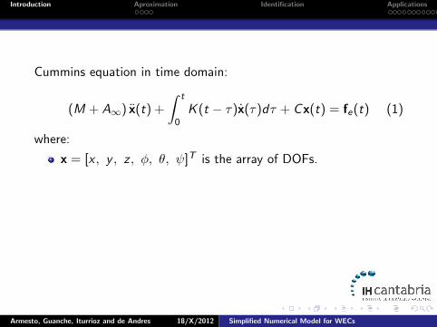
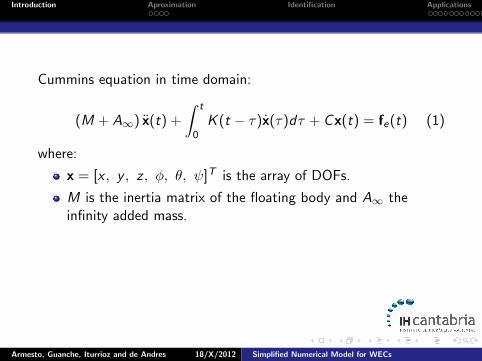
Cummins equation in time domain:
(M + A∞) x(t) +
∫ t
0K (t − τ)x(τ)dτ + Cx(t) = fe(t) (1)
where:
x = [x , y , z , φ, θ, ψ]T is the array of DOFs.
M is the inertia matrix of the floating body and A∞ theinfinity added mass.
K is the transfern function.
C is the hydrostatic matrix.
fe are the external forces applied over the body,. . .
Armesto, Guanche, Iturrioz and de Andres 18/X/2012 Simplified Numerical Model for WECs
Introduction Aproximation Identification Applications
Cummins equation in time domain:
(M + A∞) x(t) +
∫ t
0K (t − τ)x(τ)dτ + Cx(t) = fe(t) (1)
where:
x = [x , y , z , φ, θ, ψ]T is the array of DOFs.
M is the inertia matrix of the floating body and A∞ theinfinity added mass.
K is the transfern function.
C is the hydrostatic matrix.
fe are the external forces applied over the body,. . .
Armesto, Guanche, Iturrioz and de Andres 18/X/2012 Simplified Numerical Model for WECs

Introduction Aproximation Identification Applications
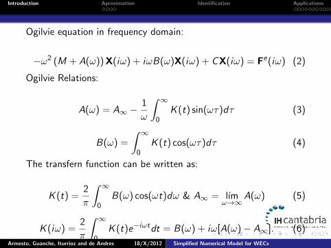
Ogilvie equation in frequency domain:
−ω2 (M + A(ω)) X(iω) + iωB(ω)X(iω) + CX(iω) = Fe(iω) (2)
Ogilvie Relations:
A(ω) = A∞ −1
ω
∫ ∞0
K (t) sin(ωτ)dτ (3)
B(ω) =
∫ ∞0
K (t) cos(ωτ)dτ (4)
The transfern function can be written as:
K (t) =2
π
∫ ∞0
B(ω) cos(ωt)dω & A∞ = lımω→∞
A(ω) (5)
K (iω) =2
π
∫ ∞0
K (t)e−iωtdt = B(ω) + iω[A(ω)− A∞]. (6)
Armesto, Guanche, Iturrioz and de Andres 18/X/2012 Simplified Numerical Model for WECs

Introduction Aproximation Identification Applications
Ogilvie equation in frequency domain:
−ω2 (M + A(ω)) X(iω) + iωB(ω)X(iω) + CX(iω) = Fe(iω) (2)
Ogilvie Relations:
A(ω) = A∞ −1
ω
∫ ∞0
K (t) sin(ωτ)dτ (3)
B(ω) =
∫ ∞0
K (t) cos(ωτ)dτ (4)
The transfern function can be written as:
K (t) =2
π
∫ ∞0
B(ω) cos(ωt)dω & A∞ = lımω→∞
A(ω) (5)
K (iω) =2
π
∫ ∞0
K (t)e−iωtdt = B(ω) + iω[A(ω)− A∞]. (6)
Armesto, Guanche, Iturrioz and de Andres 18/X/2012 Simplified Numerical Model for WECs
Introduction Aproximation Identification Applications
Data A and B is obtained by a Boundary Element Method (BEM)software WADAM/WAMIT for a given set of frequencies.
This program also provides M, C and wave forces for the given setof frequencies.
Then, we know:
A(ω) and B(ω) for ω in {ωi}Nn=1.
M and C .
Fw (ω) for ω in {ωi}Nn=1.
Armesto, Guanche, Iturrioz and de Andres 18/X/2012 Simplified Numerical Model for WECs

Introduction Aproximation Identification Applications
Convolution integrals in Cummins equation are computationallyexpensive, then we want to replace them for something moreefficient.
(M + A∞) x(t) +
∫ t
0K (t − τ)x(τ)dτ + Cx(t) = fe(t) (7)
We want to replace every convolution integral by a state-space:
α(t) = Ai ,jα(t) + Bi ,j xj(t)yi ,j(t) = Ci ,jα(t)
(8)
Such that:
yi ,j(t) ≈∫ t
0ki ,j(t − τ)xj(τ)dτ, i , j ∈ {1, 2, . . . , 6} (9)
Armesto, Guanche, Iturrioz and de Andres 18/X/2012 Simplified Numerical Model for WECs

Introduction Aproximation Identification Applications
One Degree of Freedom
Cummins equation results:
(M + A∞) z(t) +
∫ t
0K (t − τ)z(τ)dτ + Cz(t) = fe(t) (10)
Which can be written as:
(M + A∞) z(t) + yc(t) + Cz(t) = fe(t) (11)
Lets define k1(t) = z(t) y k2(t) = z(t)
k1(t) = k2(t)
k2(t) = z(t)(12)
(M + A∞) k2(t) + yc(t) + Cz(t) = fe(t) (13)
k2(t) = − yc(t)
M + A∞− C
M + A∞z(t) +
fe(t)
M + A∞(14)
Armesto, Guanche, Iturrioz and de Andres 18/X/2012 Simplified Numerical Model for WECs

Introduction Aproximation Identification Applications
One Degree of Freedom
Then, we have:
α(t) = Acα(t) + Bc x(t)
yc(t) = Ccα(t) ≈∫ t−∞ k(t − τ)x(τ)dτ
(15)
k2(t) = k1(t) (16)
k2(t) = − Cc
M + A∞α(t)− C
M + A∞x(t) +
fe(t)
M + A∞(17)
Armesto, Guanche, Iturrioz and de Andres 18/X/2012 Simplified Numerical Model for WECs
Introduction Aproximation Identification Applications
One Degree of Freedom
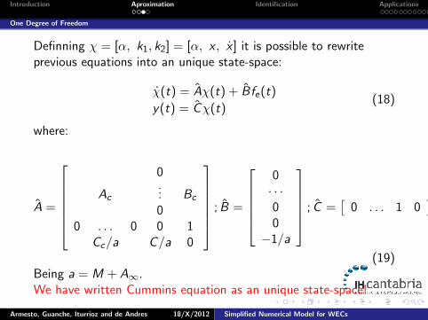
Definning χ = [α, k1, k2] = [α, x , x ] it is possible to rewriteprevious equations into an unique state-space:
χ(t) = Aχ(t) + Bfe(t)
y(t) = Cχ(t)(18)
where:
A =
0
Ac... Bc
00 . . . 0 0 1
Cc/a C/a 0
; B =
0· · ·00−1/a
; C =[
0 . . . 1 0]
(19)Being a = M + A∞.We have written Cummins equation as an unique state-space!
Armesto, Guanche, Iturrioz and de Andres 18/X/2012 Simplified Numerical Model for WECs

Introduction Aproximation Identification Applications
More than one Degree of Freedom
The same procedure can be used for more than one degree offreedom.
χ(t) =[[αc1], [αc2], . . . [αcn], [ξ], [ξ]
]T(20)
A =
[Ac1] 0 0 0 [Bc1]
0. . .
......
...... 0 [Acn] 0 [Bcn]
0... 0 0 [Id ]
[Cc1/M] . . . [Ccn/M] [G/M] 0
; B =
0...0
−[M−1
]
(21)
C =[
0 . . . 0 1 0]
(22)
Armesto, Guanche, Iturrioz and de Andres 18/X/2012 Simplified Numerical Model for WECs
Introduction Aproximation Identification Applications
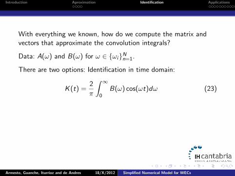
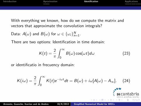
With everything we known, how do we compute the matrix andvectors that approximate the convolution integrals?
Data: A(ω) and B(ω) for ω ∈ {ωi}Nn=1.
There are two options: Identification in time domain:
K (t) =2
π
∫ ∞0
B(ω) cos(ωt)dω (23)
or identificatio in frecuency domain:
K (iω) =2
π
∫ ∞0
K (t)e−iωtdt = B(ω) + iω[A(ω)− A∞]. (24)
Armesto, Guanche, Iturrioz and de Andres 18/X/2012 Simplified Numerical Model for WECs
Introduction Aproximation Identification Applications
With everything we known, how do we compute the matrix andvectors that approximate the convolution integrals?
Data: A(ω) and B(ω) for ω ∈ {ωi}Nn=1.
There are two options: Identification in time domain:
K (t) =2
π
∫ ∞0
B(ω) cos(ωt)dω (23)
or identificatio in frecuency domain:
K (iω) =2
π
∫ ∞0
K (t)e−iωtdt = B(ω) + iω[A(ω)− A∞]. (24)
Armesto, Guanche, Iturrioz and de Andres 18/X/2012 Simplified Numerical Model for WECs

Introduction Aproximation Identification Applications
Using A(ω) and B(ω) it is possible to built the transfern functionfor every frequency ω ∈ {ωi}Nn=1:
K (iωj) = B(ωj) + iωj (A(ωj)− A∞) (25)
A Matlab Toolbox done by Perez and Fossen, compute valuesθ = [p0, p1, . . . , pn−1, q0, q1, . . . , qn−1] such that:
K (s, θ) =pn−1s
n−1 + pn−2sn−2 + . . .+ p1s
1 + p0sn + qn−1sn−1 + qn−2sn−2 + . . .+ q1s1 + q0
(26)
is the best possile approximation (least square sense) for K (iω),ω ∈ {ωi}Nn=1
This means that this toolbox provides element θ? that minimizesthe following operatos:
θ? = mınθ
(∑n
(K (iωn)− K (iωn, θ)
)2)(27)
Armesto, Guanche, Iturrioz and de Andres 18/X/2012 Simplified Numerical Model for WECs
Introduction Aproximation Identification Applications
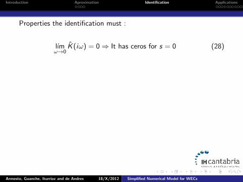
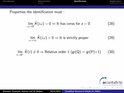
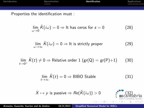
Properties the identification must :
lımω→0
K (iω) = 0⇒ It has ceros for s = 0 (28)
lımω→∞
K (iω) = 0⇒ It is strictly proper (29)
lımt→0+
K (t) 6= 0⇒ Relative order 1 (gr(Q) = gr(P)+1) (30)
lımt→∞
K (t) = 0⇒ BIBO Stable (31)
X 7→ y is passive⇒ Re(K (iω)) > 0 (32)
Armesto, Guanche, Iturrioz and de Andres 18/X/2012 Simplified Numerical Model for WECs

Introduction Aproximation Identification Applications
Properties the identification must :
lımω→0
K (iω) = 0⇒ It has ceros for s = 0 (28)
lımω→∞
K (iω) = 0⇒ It is strictly proper (29)
lımt→0+
K (t) 6= 0⇒ Relative order 1 (gr(Q) = gr(P)+1) (30)
lımt→∞
K (t) = 0⇒ BIBO Stable (31)
X 7→ y is passive⇒ Re(K (iω)) > 0 (32)
Armesto, Guanche, Iturrioz and de Andres 18/X/2012 Simplified Numerical Model for WECs
Introduction Aproximation Identification Applications
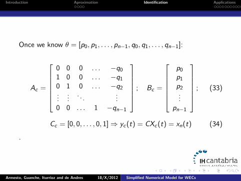
Once we know θ = [p0, p1, . . . , pn−1, q0, q1, . . . , qn−1]:
Ac =
0 0 0 . . . −q01 0 0 . . . −q10 1 0 . . . −q2...
.... . .
...0 0 . . . 1 −qn−1
; Bc =
p0p1p2...
pn−1
; (33)
Cc = [0, 0, . . . , 0, 1]⇒ yc(t) = CXc(t) = xn(t) (34)
.
Armesto, Guanche, Iturrioz and de Andres 18/X/2012 Simplified Numerical Model for WECs

Introduction Aproximation Identification Applications
CatAir
Armesto, Guanche, Iturrioz and de Andres 18/X/2012 Simplified Numerical Model for WECs
Introduction Aproximation Identification Applications
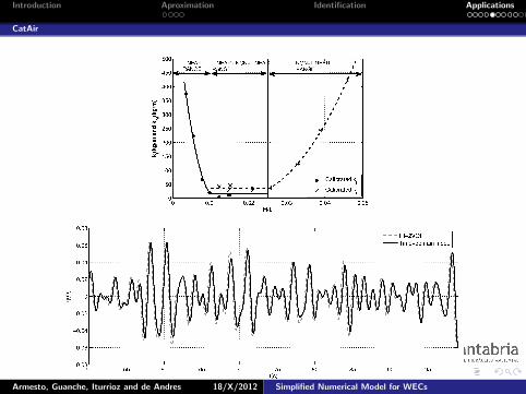
CatAir
Armesto, Guanche, Iturrioz and de Andres 18/X/2012 Simplified Numerical Model for WECs

Introduction Aproximation Identification Applications
CatAir
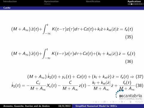
(M + A∞) z(t)+
∫ t
−∞K (t−τ)z(τ)dτ+Cz(t)+kl z+knl |z |z = fe(t)
(35)
(M + A∞) z(t)+
∫ t
−∞K (t−τ)z(τ)dτ+Cz(t)+(kl + knl |z |) z = fe(t)
(36)
(M + A∞) k2(t) + yc(t) + Cz(t) + (kl + knl z) z = fe(t)⇒ (37)
k2(t) = − Cc
M + A∞Xc(t)− C
M + A∞z(t)− kl + knl |z |
M + A∞z +
fe(t)
M + A∞(38)
Armesto, Guanche, Iturrioz and de Andres 18/X/2012 Simplified Numerical Model for WECs

Introduction Aproximation Identification Applications
CatAir
(M + A∞) z(t)+
∫ t
−∞K (t−τ)z(τ)dτ+Cz(t)+kl z+knl |z |z = fe(t)
(35)
(M + A∞) z(t)+
∫ t
−∞K (t−τ)z(τ)dτ+Cz(t)+(kl + knl |z |) z = fe(t)
(36)
(M + A∞) k2(t) + yc(t) + Cz(t) + (kl + knl z) z = fe(t)⇒ (37)
k2(t) = − Cc
M + A∞Xc(t)− C
M + A∞z(t)− kl + knl |z |
M + A∞z +
fe(t)
M + A∞(38)
Armesto, Guanche, Iturrioz and de Andres 18/X/2012 Simplified Numerical Model for WECs
Introduction Aproximation Identification Applications
CatAir
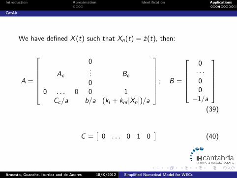
We have defined X (t) such that Xn(t) = z(t), then:
A =
0
Ac... Bc
00 . . . 0 0 1
Cc/a b/a (kl + knl |Xn|)/a
; B =
0· · ·00−1/a
(39)
C =[
0 . . . 0 1 0]
(40)
Armesto, Guanche, Iturrioz and de Andres 18/X/2012 Simplified Numerical Model for WECs
Introduction Aproximation Identification Applications
CatAir
Armesto, Guanche, Iturrioz and de Andres 18/X/2012 Simplified Numerical Model for WECs

Introduction Aproximation Identification Applications
CatAir
mair = − d
dt(ρair (t)Vair (t)); Vair (t) = V0 − Sz(t) = S(L0 − z(t)).
(41)Assuming the proccess is isentropic, ρair (t)(P0 + ∆P(t))−1/γ = KThe air mass flux through the openning can be expressed asfollows:
mair (t) = cdAv sgn(∆P(t))
[2mair (t)|∆P(t)|
Vair (t)
]1/2(42)
Armesto, Guanche, Iturrioz and de Andres 18/X/2012 Simplified Numerical Model for WECs

Introduction Aproximation Identification Applications
CatAir
Lets define the relative pressureP∗(t) = P(t)/P0 = (∆P(t) + P0)/P0.The air pressure variation inside the chamber,
P∗(t) =
[−Avcdγkv
ρ0Ssgn(P∗(t)− 1)
(2P0ρ0P
∗(t)−1/γ |P∗(t)− 1|)1/2
+γz(t)]P∗(t) = ΓP∗(t) (43)
Cummins’ equation as solved using a state-space,
X (t) = AX (t) + Bu(t)y(t) = CX (t)
(44)
Cummins’ equation is modified to include pressure effects,
(m + A∞)z(t) + yc(t) + ρgSz(t) + kz(t)−∆P(t)S = fe(t) (45)
Armesto, Guanche, Iturrioz and de Andres 18/X/2012 Simplified Numerical Model for WECs

Introduction Aproximation Identification Applications
CatAir
Writting together equations (45) and (43), we can write a newstate-space.The first step is to redefine the space’s vector,
X (t) =[X (t) P∗(t)
]. (46)
Then matrix A and arrays B and C are redefined as:
A =
0
A 0−S
0 . . . 0 Γ
;B =
B
0
;C =[C 0
]. (47)
Armesto, Guanche, Iturrioz and de Andres 18/X/2012 Simplified Numerical Model for WECs
Introduction Aproximation Identification Applications
CatAir
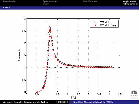
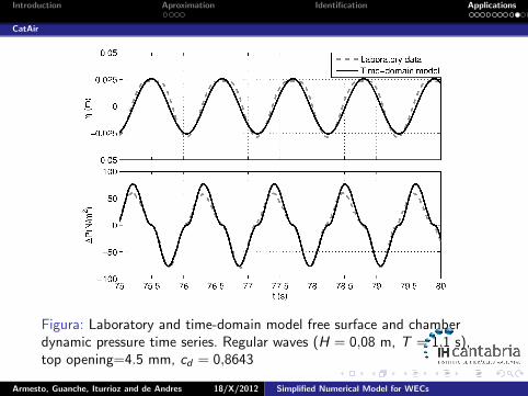
Figura: Laboratory and time-domain model free surface and chamberdynamic pressure time series. Regular waves (H = 0,08 m, T = 1,1 s),top opening=4.5 mm, cd = 0,8643
Armesto, Guanche, Iturrioz and de Andres 18/X/2012 Simplified Numerical Model for WECs
Introduction Aproximation Identification Applications
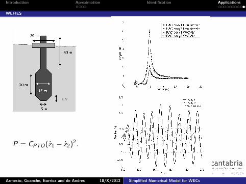
WEFIES
P = CPTO(z1 − z2)2.
Armesto, Guanche, Iturrioz and de Andres 18/X/2012 Simplified Numerical Model for WECs
Introduction Aproximation Identification Applications
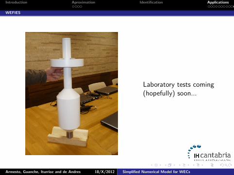
WEFIES
Laboratory tests coming(hopefully) soon...
Armesto, Guanche, Iturrioz and de Andres 18/X/2012 Simplified Numerical Model for WECs

Introduction Aproximation Identification Applications
WEFIES
Thanks for yourattention!
Armesto, Guanche, Iturrioz and de Andres 18/X/2012 Simplified Numerical Model for WECs