Simple Tool for Semi-automated Evaluation of Yeast Colony ...

Simple Tool for Semi-automated Evaluationof Yeast Colony Images

Jan Schier and Bohumil Kovar

Institute of Information Theory and Automation of the ASCRPod vodarenskou vezı 4, CZ-182 08 Prague 8, Czech Republic

{schier,kovar}@utia.cas.cz

Abstract. A tool for semi-automated evaluation of images of yeast colonies ispresented in the paper. The input data for the tool is a batch of Petri dish images,possibly in nested directories, the output is written to a text file in a simple CSV(comma-separated values) format. The tool is designed to evaluate, for each dishimage, the relative coverage of the dish and the number of colonies contained inthe dish. It is intended for use in a research laboratory, where a general-purposeimaging setup is used to take the images, which are then processed off-line.

In the paper, the characteristic features of the yeast colony images are de-scribed and the processing flow and the user interface of the tool are reviewed.The performance of the counting is evaluated using a test set of 245 images withtypical relative coverage of less than 10%.

The tool is available for download from our web page.

1 Introduction

Yeast, namely Saccharomyces cerevisiae, is often used as a model organism in biolo-gical research. This is mainly due to its many favourable properties, such as the shortgeneration time, easy genetical manipulation, as well as thanks to its established use inindustry.

When performing experiments with S. Cerevisiae yeast, part of the process is grow-ing the yeast colonies in Petri dishes, and evaluating the growth parameters, such as thecoverage of the dish and the number of colonies. Traditionally, the colonies have beencounted manually, using either manual colony counter or a counting raster. Examples ofthe manual counters are the Colony counter SC6 by Stuart1 or the EW-14211-02 Hand-Held Electronic Colony Counter from Cole-Parmer2. However, the hand counting isconsidered rather laborious and time-consuming process, error prone due to the fatigueand eye-strain of the technician. Also, it does not provide any figures on the coverageof the dish or the radii of the colonies.

There are also a number of automated colony counters available – it is of interest thatsuch system has been described as early as in 1974 [1]. An automated counter usuallyconsists of a single-purpose chamber with an illumination and camera system, wherethe dishes are placed either manually one-by-one or by an automated plate-handler,

1 www.stuart-equipment.com2 www.coleparmer.com

A. Fred, J. Filipe, and H. Gamboa (Eds.): BIOSTEC 2011, CCIS 273, pp. 110–125, 2012.c© Springer-Verlag Berlin Heidelberg 2012

Simple Tool for Semi-automated Evaluation 111

and of a computer running an image-processing program that performs thresholding,segmentation, and statistical evaluation of the image.

An automated counter is definitely the system-of-choice for a commercial lab. Oursystem, however, has been developed for a the cooperating university research lab. Therequirements were not only that it performs adequately for typical image variations, butalso – quite importantly – to reuse the imaging equipment already available in the lab(to achieve a low-cost solution), and to provide an off-line batch processing of a set ofimages taken beforehand in the darkroom. Additionally, the tool should operate withminimum possible manual intervention of operator, while allowing for manual correc-tion of the counting errors (multiple detections of a single colony or missed colonies).Finally, it should provide not only the count of colonies, but also evaluate the totalcoverage of the dish.

Finally, the open-source framework ImageJ [2] should be noted in the context ofexisting tools. It is a feature-rich tool for image processing, with focus in medical andbiological applications. In the field of our interest, it provides many algorithms for im-age thresholding and segmentation. In our view, however, it is targeted more generallyand to prepare a specialized application which shields the user of the complexity ofthe underlying system would require an effort similar to development of our solution.We have decided to use MATLAB with the Image processing toolbox, because of ourprevious experience with that environment.

In the paper, we describe the processing flow of our tool and present the performancedata that we have achieved. The paper is structured in the following way: in Section 2,the characteristics of typical images are reviewed. In Section 3, the components of thesystem are discussed. Section 5 describes the experiments and performance results.Finally, Section 6 concludes the paper.

2 Characteristics of Typical Images

As has been stated, the requirement on our system was that it should be able to processbatches of images taken with a simple general-purpose imaging system; the laboratoryis using a camera/copy stand with lightning units by Kaiser Fototechnik3 (see Fig. 1).The dishes are manually placed roughly into the center of the image, on a mat blackbackground. No dish holder or stopper is used.

Examples of typical images of yeast colonies are shown in Figure 2. The images arecharacterized by the following properties:

– dark background to increase image contrast– illumination by two linear light sources along the short edges (this is not important

for processing, though)– variations of dish position – cf. Figure 2a and 2b– varying diameter of the dish image and varying intensity of the dish background

(both depend on the adjustment on the imaging setup in the particular session)

The colonies selves are characterized by differing types of morphologies (smooth orfluffy), colony size dispersion (even within single dish) and by colonies often touching

3 www.kaiser-fototechnik.de

112 J. Schier and B. Kovar

Fig. 1. General-purpose imaging setup used with the proposed colony counter

(a) Fluffy and touching colonies,diverse radii, dish centered.

(b) Smooth colonies, dish touchingedge of image.

Fig. 2. Examples of typical images of yeast colonies

each other. Let us note that the morphology and size of colonies depends both on theirage and on the growth conditions.

3 System Description

Counting of colonies typically consists of several operations, which follow from theimage characteristics[3,4]. This operations include image thresholding, dish localiza-tion, and the counting self. In this paper, we divide the processing into two basic parts– image preprocessing and colony counting.


3.1 Image Preprocessing

The goal of this step is to determine the exact position of the dish in the image, todetermine the area of the dish, and to extract the image of colonies and measure it’ssurface, so that the relative coverage can be determined. The image is checked for anyfaults in this step, such as missing parts (see Fig. 3a) or corrupted background (Fig. 3b).Let us note that while the missing part makes it impossible to determine properly thetotal area of the dish, the corrupted background can be eliminated to some extent.

(a) Missing part of the dish. (b) Corrupted background.

Fig. 3. Examples of faulty images

The processing flow of the preprocessing is outlined in Fig. 4 on the following page.It starts with operations related to dish localization: the image is first binarized. A thresh-old that is used in this process is computed using samples from the image corners.Let these samples be S1, . . . ,S4 (see Fig. 5 on the next page), with the mean valuesS1, . . . , S4 and the standard deviations σ1, . . . ,σ2. The background threshold θb is de-rived from the sample with minimum mean value:

i = argmini(Si) , θb = Si + 3σi + offset

Note: offset is used to ensure that the threshold will be set above the peaks of thebackground sample. In our implementation, we use offset equal to 5.

Next step is to project the binary image along the horizontal and vertical axis. Theprojections Px and Py of the binary image Ib are given as the pixel sum in the givendirection:

Px = ∑j

Ib, j ,

Py = ∑i

Ib,i ,

where i is the row index and j is the column index.The dish is, in these projections, manifested as a broad ’lobe’, or peak (see

Fig. 6 on page 115). The partly uncovered background – if present – would show upas another peak (cf. the graphs in the bottom row of Fig. 6 on page 115), however, the


Backgroundsamples

Backgroundthreshold

computation

Input image I

Backgroundthresholding

ProjectionsDish

position

Imagechecking

Rejectedimages

Binaryimage Ib

Dishlocalization

Dish masking

Dishposition

Otsuthreshold

computation

Thresholdadjustment

usinghistogram

CenteredDish

Extractionof colonies

Extracted colonies

Fig. 4. Processing flow of dish preprocessing

S3

S2S1

S4

Fig. 5. Position of image background samples

lobe corresponding with the dish is the broadest one. Additional check for uniformity ofestimated diameters in horizontal and vertical direction is applied to eliminate heavilycorrupted images.


Correct image Corrupted background

Original image.

Binary image.

Dish projection along vertical axis.

Fig. 6. Computation of dish projection Py – example

Finally, the dish is approximated by a circle with the center and diameter derivedfrom the edges determined in the dish localization step. The result of the preprocessingis a centered image of the dish, with eliminated background. An illustrative example isgiven in Fig. 7 on the following page.

The last step of the image preprocessing is the extraction of colonies, which is usedto assess the total covered area, in order to determine the relative coverage of the dish.A new threshold is used in this step, located between the brightness levels of the dishbackground and of the colonies, as close as possible to the background.


Fig. 7. Dish image after preprocessing

The most straightforward solution is to use the well-established Otsu threshold-ing [5]. However, the threshold based purely on this method may be set too high, if thecolony edge is fading gradually. To avoid this, we have introduced a histogram-basedcorrection to the method (see Fig. 8 on the next page and Fig. 9 on page 118).

The principle of this correction is following: first, by limiting the histogram by theOtsu threshold θO, we cut-off the part corresponding with (brighter) colonies. The peakof the remaining part (Fig. 9) corresponds with the dish background. The thresholdshould be placed just above the right edge of this peak.

More formally, let H = [h1, . . . ,hO] be the histogram of the pixels below the Otsuthreshold θO. Let HMA be histogram filtered by a moving average filter:

HMA = [hMA,1, . . . ,hMA,O], hMA,i = (N

∑j=1

hi− j+1)/N, i− j+ 1 < 0 : hi− j+1 = 0.

Let ΔHMA be the first difference of the filtered histogram. Then, the dish threshold withcorrection θd is given as

θd = max(i), ΔHMA(i)<−sd,

where sd is a user-selected setpoint. In our implementation, we use N = 4 and sd = 100,with good thresholding performance.

3.2 Colony Counting

In this step, the centered image of the colonies, resulting from preprocessing, is used tofind the individual colonies.

The simplest approach to counting is to correlate the contour of the colonies witha circular pattern, assuming that the maxima of correlation are located at the centersof colonies. This has been the first method we have tested. During experiments, we


Fig. 8. Dish thresholding - pure Otsu method and a histogram-based correction

have experienced poor performance in the case of big clusters (the error rate of ourimplementation was reaching up to 30%) and sensitivity to mismatch between the radiusof the circular pattern diameter and the radius of the colony (and, hence, sensitivity todispersion of colony radii).

An interesting approach to the counting of bacteria colonies has been describedin [3]: to find colonies, a number of shape and structure criteria are used on the


Fig. 9. Position of Otsu threshold and of threshold with correction relative to histogram

image pixels, including e.g. mean object radius, roundness of an object, compactnessand asymmetry, radial monotony of fall-off in intensity, etc. These criteria are com-bined into shape and structure quality parameters and evaluated using fuzzy logic. Themethod works best under the assumptions of well-defined circular shape and monotoneintensity fall-off of the colonies, which are well satisfied for bacteria (the case treated inthe work of Marotz), but not necessarily in our case of the yeast colonies (for examplesof possible morphologies see e.g. [6,7]).

A popular method to detect circular objects is the circular Hough transform (for defi-nition see e.g. [8]). Based on our experiments, if multiple yeast colonies are overlappingor touching, it tends to detect (incorrectly) adjacent colonies as a single object. Also,following the results presented in [9], the output of the Hough transform may be rathernoisy.

Another possibility is to use the methods based on radial symmetry – the radialsymmetry transform has been introduced in [10].

Fast Radial Transform. In our solution, we use the Fast radial transform – a modifiedversion of the radial symmetry transform, first presented in [9]. It is a transform thatmaps the original image to the transformed image according to its contribution to radialsymmetry of the gradients at distance n∈ N (N is the set of radii) away from each point.For full details of the method see the original description.

First, image gradient gi, j at each point (i, j) is calculated. Then, the positively- andnegatively affected pixels are determined. An affected pixel is defined as the point eitherin- or counter the direction of the gradient vector gi, j, at a distance n pixels away fromthe point at coordinates (i, j). The coordinates of affected pixels are given by

p+(i, j) = (i, j)+ round

(gi, j

‖gi, j‖n

),


p−(i, j) = (i, j)− round

(gi, j

‖gi, j‖n

).

The gradient matrix g, together with the coordinates of affected pixels, is used to de-termine the orientation and magnitude projection images On and Mn for the givenradius n:

On(p+(i, j)) = On(p+(i, j))+ 1 ,

On(p−(i, j)) = On(p−(i, j))− 1 ,

Mn(p+(i, j)) = Mn(p+(i, j))+ ‖gi, j‖ ,

Mn(p−(i, j)) = Mn(p−(i, j))−‖gi, j‖ .

The radial symmetry at radius n is defined by convolution of matrices

Sn = Fn ∗An ,

where the elements

Fn(i, j) =Mn(i, j)

kn

( |On(i, j)|kn

)α

,

and

On(i, j) =

{On(i, j) if On(i, j) < kn ,

kn otherwise .

Here, An is a two-dimensional Gaussian, α is the so-called radial strictness parame-ter and kn is a scaling factor used to normalize Mn and On (for settings used in ourimplementation see 5.1). Projection images Mn and On are initially set to zero.

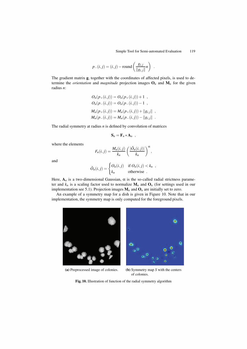
An example of a symmetry map for a dish is given in Figure 10. Note that in ourimplementation, the symmetry map is only computed for the foreground pixels.

(a) Preprocessed image of colonies. (b) Symmetry map S with the centersof colonies.

Fig. 10. Illustration of function of the radial symmetry algorithm


Colony Radius Estimation. Let us recall that there are often colonies with differentradii contained in a single dish (see Sec. 2). Hence, prior to the radial transform compu-tation, the set of radii N of the colonies in the dish is to be estimated, using the followingprocedure:

– the equivalent diameter d and eccentricity ε is computed for each object in theimage. The diameter is derived from area A (number of pixels) of an object. Theeccentricity equals to the eccentricity of an ellipse with the same second momentsas the object. It ranges from ε = 0 for a circle to ε = 1 for a line segment.

– Nearly circular objects (with eccentricity ε< θε, where θε is the eccentricity thresh-old), are selected.

– Min and max diameter dmin and dmax of the objects in the set of circular objects aredetermined. The interval between them is divided to ν equidistant subintervals. Theset of radii N for the fast radial transform is then given by:

Δ = dmax − dmin

N = {dmin +[0, . . . ,ν] ·Δ/ν}/2

Estimation of Colony Centers. The centers of the colonies are represented by localmaxima of the symmetry matrix S, which are detected using the the nonmaxsuppts()function described in [11]. The output of this function are the coordinates of the centers.

4 Counting Tool

The processing flow, as described in Section 3, has been implemented in a countingtool (Fig. 11 on the next page). It performs fully automatic thresholding of the image,localization of the dish and counting of colonies. The tool provides an environment forselection of the directory tree with images to process, of the file to store the countingresults, and of the counting mode: in the semi-automatic mode, a simple point-and-clickeditor can be used for manual correction of the system output, in the fully-automaticmode, the output of the system is directly stored into the result file. This tool was usedalso to obtain the reference results used in this paper: using manual correction, weobtained the ground-truth counts of colonies in Petri dishes, which were used to evaluatethe counting error rates.

5 Experiments and Results

To evaluate the system recognition performance, it has been tested using a set of 245images, containing colonies with different morphology and relative coverage of thedish. The distribution of the test set in the terms of frequencies of the number of coloniesin the dish is shown in Fig. 12a. Figure 12b shows the distribution of relative coverageof the dish and mean diameter of colonies (marker size) in comparison with the numberof colonies in the dish. In the set, the minimum and maximum counts were 8 and 95colonies per dish, when 80% of dishes contained less than 50 colonies. The minimumand maximum coverage were 0.43% and 25.3%, respectively, and 80% of dishes hadcoverage up to 8.26%.


Fig. 11. Counting application

0–

1010

–20

20–

3030

–40

40–

5050

–60

60–

7070

–80

80–

9090

–10

0

0

20

40

60

80

1

47

83

35 33

2113

4 62 0

Number of Colonies

Num

ber

ofsa

mpl

es(d

ishe

s)

(a) Histogram of dish sample distribution.

0 20 40 60 80 100

0

10

20

Number of colonies

Rel

ativ

eco

vera

ge[%

]

(b) Relative dish coverage related to the number of colonies.Diameter of markers represents mean radius of thecolonies in the dish.

Fig. 12. Distribution of the test set

5.1 Algorithm Settings

The following settings were used in our experiments:

– Parameters of the fast radial transform:

kn = 6, α = 4

Let us note that setting α = 2 (see Sec. 5.1) could be better choice – the responseof the radial transform on fluffy colonies with less circular shape would be higher


and the computational demands of the method would be somewhat lower. However,all experimental data presented later have been obtained for α = 4. We have per-formed a test with α = 2 on a randomly selected sample of 15 images. The countingperformance has been slightly improved, however, the system was more sensitiveto the background noise along the dish edge (giving numerous false positives insome cases). The problem of elimination of the reflections on the dish edge hasbeen treated e.g. in [4]; we perform only simple reduction of the dish radius, whichshould cover the dish lip region.

– Parameters of the non-maxima suppression nonmaxsuppts() [11]:

thresh = 4, radius = 0.8 ·min(N),

where N is the set of radii for the fast radial transform.– Construction of N: eccentricity threshold θε (see Section 3.2) is initially set to θε =

0.25. The number of equidistant intervals ν is set to ν = 4. At least five colonies ofgiven eccentricity must be in the image, else the eccentricity is increased by stepof 0.1 (we start from stricter requirement on circularity of colonies, to eliminateclusters. If there are not enough colonies of the given circularity, we loosen thecriterion and accept those with less circular shape).Let us note that the distribution of colony diameters should also be considered,however, this is not implemented in the tool at the moment.

5.2 Typical Detection Errors

Figure 13 illustrates typical detection errors of fast radial transform. A colony may bemissed if it touches other colony or multiple colonies, so that they form a cluster. Thisdetection error is almost absent if the colonies touch only at one point, creating a chain-like structure. More colonies touching each other form a structure in which their shapeis distorted and internal colonies cease to be circular. The circular outer border of colonylocated in such cluster could be too short for the proposed method to work properly.

Fig. 13. Example of typical detection error of fast radial transform

5.3 Counting Performance

The counting errors for various number of colonies are summarized inTab. 1 on the facing page. The relatively high counting error for the dishes with thecolony counts greater than 60 is given by two factors. First, with the increasing num-ber of colonies increases also the probability that there will be colonies touching eachothers (Fig. 13). Second, the number of samples with this high density of coverage wasrelatively low, thus increasing the evaluation error (Fig. 12a on the previous page).


Table 1. Dependence of the counting errors on the number of colonies in the dish. The systemaverage counting error is under 4%.

� colonies samples missed [%] false [%]

0 – 17 21 1.47 018 – 20 19 2.99 021 – 23 25 3.31 024 – 26 29 4.00 027 – 29 27 3.28 030 – 40 35 4.17 041 – 49 30 4.00 050 – 60 29 3.87 2.00> 60 30 5.36 3.22

20 40 60 80 100

20

40

60

80

100

Number of colonies

Num

ber

ofde

tect

edco

loni

es

Fig. 14. Algorithm recognition performance related to the number of colonies

0–20 20–40 40–60 > 600

10

20

30

Number of colonies

Mis

sed

colo

nies

(nor

mal

ized

)[%

]

# colonies samples0–20 40

20–40 12340–60 52>60 30

Fig. 15. Relative number of missed colonies dependent on the number of colonies


Figure 14 on the preceding page shows the recognition performance related to thenumber of colonies in the dish. The dishes, where some colonies have been missed fallbelow the dashed line.

Another view on the algorithm performance is provided by Fig. 15, which presentsa box-whisker plot of relative counting error (missed colonies) in several groups of thecolony counts. The numbers of samples per group are given in the attached table.

6 Conclusions

In the paper, we have presented the tool for evaluation of yeast colony images, targetedtowards batch processing of images prepared with a general-purpose imaging system.The processing flow of the system has been described. The performance of the tool hasbeen tested on a set of 245 images with different degrees of coverage. The distributionof the data in the test set and the performance of the system have been discussed. Theaverage counting error is below 4%. It is difficult to compare the performance with thecommercial solutions, since the performance data of these systems are not available.

There are still performance challenges, especially in resolution of clustered fluffycolonies. The resolution of clustered colonies is rather common problem, reported alsoin other works [4]. The performance, however, has been acceptable for our target labo-ratory user.

The application has been implemented in a Matlab. This tool has been successfullydeployed in the cooperating biology research laboratory and is available for download4.

Acknowledgements. This research has been supported from the TA01010931 ”Systemfor support of the FISH method evaluation” project of the Technology Agency of theCzech Republic.

We would like to thank the staff of the Yeast Colony Group, Department of Geneticsand Microbiology, Faculty of Sciences, Charles University, who have introduced us intothe problem and provided us with the sample images from their experiments.

References

1. Goss, W.A., Michaud, R.N., McGrath, M.B.: Evaluation of an automated colony counter.Appl. Microbiol. 27, 264–267 (1974)

2. Burger, W., Burge, M.J.: Digital Image Processing: An Algorithmic Introduction using Java.Springer, Heidelberg (2007)

3. Marotz, J., Lubert, C., Eisenbeiss, W.: Effective object recognition for automated countingof colonies in petri dishes (automated colony counting). Computer Methods and Programs inBiomedicine 66, 183–198 (2001)

4. Chen, W.B., Zhang, C.: An automated bacterial colony counting and classification system.Information Systems Frontiers 11, 349–368 (2009)

5. Otsu, N.: A Threshold Selection Method from Gray-Level Histograms. IEEE Transactionson Systems, Man, and Cybernetics 9, 62–66 (1979)

4 http://zs.utia.cz/index.php?ids=results&id=yeastcolcount&lang=eng


6. Granek, J.A., Magwene, P.M.: Environmental and genetic determinants of colony morphol-ogy in yeast. PLoS Genetics 6, e1000823 (2010)

7. St’ovıcek, V., Vachova, L., Kuthan, M., Palkova, Z.: General factors important for the for-mation of structured biofilm-like yeast colonies. Fungal Genetics and Biology: FG & B 47,1012–1022 (2010)

8. Ballard, D.H., Brown, C.M.: Computer Vision. Online Book (2003)9. Loy, G., Zelinsky, A.: Fast radial symmetry for detecting points of interest. IEEE Transac-

tions on Pattern Analysis and Machine Intelligence 8, 959–973 (2003)10. Reisfeld, D., Wolfson, H., Yeshurun, Y.: Context-free attentional operators: The generalized

symmetry transform. International Journal of Computer Vision 14, 119–130 (1995)11. Kovesi, P.D.: MATLAB and Octave functions for computer vision and image processing.

School of Computer Science & Software Engineering, The University of Western Australia(2005), http://www.csse.uwa.edu.au/˜pk/research/matlabfns/

http://www.csse.uwa.edu.au/~pk/research/matlabfns/

Simple Tool for Semi-automated Evaluation of Yeast Colony ...

Documents

Transcript of Simple Tool for Semi-automated Evaluation of Yeast Colony ...