Progress In Electromagnetics Research M, Vol. 55, 109–119, 2017

Simple Calibration Technique for Phased Array Radar Systems

Galina Babur1, 2, *, Gleb O. Manokhin1, Evgeniy A. Monastyrev3,Andrey A. Geltser1, and Alexander A. Shibelgut1, 4

Abstract—This paper presents a novel effective calibration technique applicable to phased array radars.The real embedded patterns of the array elements are measured independently in operating mode, takingantenna coupling and other parasitic effects into account. The proposed calibration technique requiresminimal modification of the radar hardware. A set of angular-dependent error coefficients, which arecompensated during the calibration process, are extracted for one received pulse for one/each angulardirection of interest. The performance and effectiveness of the here-proposed calibration technique areassessed by means of modeling and experimental verification.

1 Introduction

2 Received Signal Model

3 Calibration Technique3.1 Description3.2 Important Notes

4 Validation of the Proposed Calibration Technique

5 Conclusion

Acknowledgment

References

1. INTRODUCTION

In phased array radars with electronic beam-steering, excitation phase and amplitude of the arrayelements are adjusted electronically in order to shape and point the array pattern along the desireddirection [1, 2]. Phase and amplitude errors introduced in the beam-forming network can lead to adegradation of the array pattern characteristics in terms of increased sidelobe level and reduction ofpeak directivity [3, 4]. Coupling is present in all antenna arrays to some extent and can significantlyaffect their operation [5]. Besides, the non-ideality of the radiation pattern featured by the individualarray elements results in a non-uniform radiation/reception of the radio signal along different angulardirections [6].

Calibration is necessary because it reduces the array errors. The smaller the array errors are, thecloser the implemented radiation pattern is to the theoretical pattern of the phased array.

Received 12 October 2016, Accepted 8 February 2017, Scheduled 23 March 2017* Corresponding author: Galina Babur (galinababur@gmail.com).1 Department of Telecommunications and Radio-engineering Fundamentals, TUSUR, 40 Lenin Avenue, Tomsk, Russia. 2 SimonStevin Institute for Geometry, Nottebohmstraat 8, 2018 Antwerpen, Belgium. 3 Institute of Semiconductor Devices (NIIPP), Tomsk,Russia. 4 Department of Computer Measuring Systems and Metrology, TPU, 30 Lenin Avenue, Tomsk, Russia.

110 Babur et al.

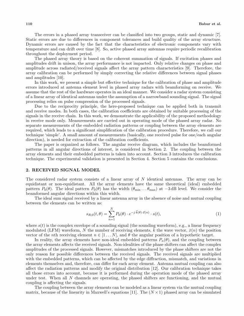
The errors in a phased array transceiver can be classified into two groups, static and dynamic [7].Static errors are due to differences in component tolerances and build quality of the array structure.Dynamic errors are caused by the fact that the characteristics of electronic components vary withtemperature and can drift over time [8]. So, active phased array antennas require periodic recalibrationthroughout the deployment period.

The phased array theory is based on the coherent summation of signals. If excitation phases andamplitudes drift in unison, the array performance is not impacted. Only relative changes on phase andamplitude across radiated/received signals affect the array pattern characteristics [9]. Therefore, thearray calibration can be performed by simply correcting the relative differences between signal phasesand amplitudes [10].

In this work, we present a simple but effective technique for the calibration of phase and amplitudeerrors introduced at antenna element level in phased array radars with beamforming on receive. Weassume that the rest of the hardware operates in an ideal manner. We consider a radar system consistingof a linear array of identical antennas under the assumption of a narrowband sounding signal. The signalprocessing relies on pulse compression of the processed signals.

Due to the reciprocity principle, the here-proposed technique can be applied both in transmitand receive modes. In both cases, the calibration coefficients are obtained by suitable processing of thesignals in the receive chain. In this work, we demonstrate the applicability of the proposed methodologyin receive mode only. Measurements are carried out in operating mode of the phased array radar. Noseparate measurements of the embedded radiation patterns or coupling between the array elements arerequired, which leads to a significant simplification of the calibration procedure. Therefore, we call ourtechnique ‘simple’. A small amount of measurements (basically, one received pulse for one/each angulardirection), is needed for extraction of the calibration coefficients.

The paper is organized as follows. The angular receive diagram, which includes the beamformedpatterns in all angular directions of interest, is considered in Section 2. The coupling between thearray elements and their embedded patterns is taken into account. Section 3 introduces the calibrationtechnique. The experimental validation is presented in Section 4. Section 5 contains the conclusions.

2. RECEIVED SIGNAL MODEL

The considered radar system consists of a linear array of N identical antennas. The array can beequidistant or non-equidistant. All the array elements have the same theoretical (ideal) embeddedpattern P0(θ). The ideal pattern P0(θ) has the width (θmin . . . θmax) at −3 dB level. We consider thebeamformed angular directions within this width.

The ideal sum signal received by a linear antenna array in the absence of noise and mutual couplingbetween the elements can be written as:

sR,0(t, θ) =N∑

n=1

P0(θ) · e−j �k(θ)·�x(n) · s(t), (1)

where s(t) is the complex envelope of a sounding signal (the sounding waveform), e.g., a linear frequencymodulated (LFM) waveform, N the number of receiving elements, k the wave vector, x(n) the positionvector of the nth receiving element n ∈ [1 . . . N ], and θ the angular position of a hypothetic target.

In reality, the array elements have non-ideal embedded patterns Pn(θ), and the coupling betweenthe array elements affects the received signals. Non-idealities of the phase shifters can affect the complexamplitudes of the processed signals. However, mismatches introduced by the phase shifters are not theonly reason for possible differences between the received signals. The received signals are multipliedwith the embedded patterns, which can be affected by the edge diffraction, mismatch, and variations inelements themselves and, therefore, can differ for each array element. Antenna mutual coupling can alsoaffect the radiation patterns and modify the original distribution [12]. Our calibration technique takesall those errors into account, because it is performed during the operation mode of the phased arrayunder test. When all N channels are operating, the phased shifters are functioning, and the mutualcoupling is affecting the signals.

The coupling between the array elements can be modeled as a linear system via the mutual couplingmatrix, because of the linearity in Maxwell’s equations [11]. The (N ×1) phased array can be simulated

Progress In Electromagnetics Research M, Vol. 55, 2017 111

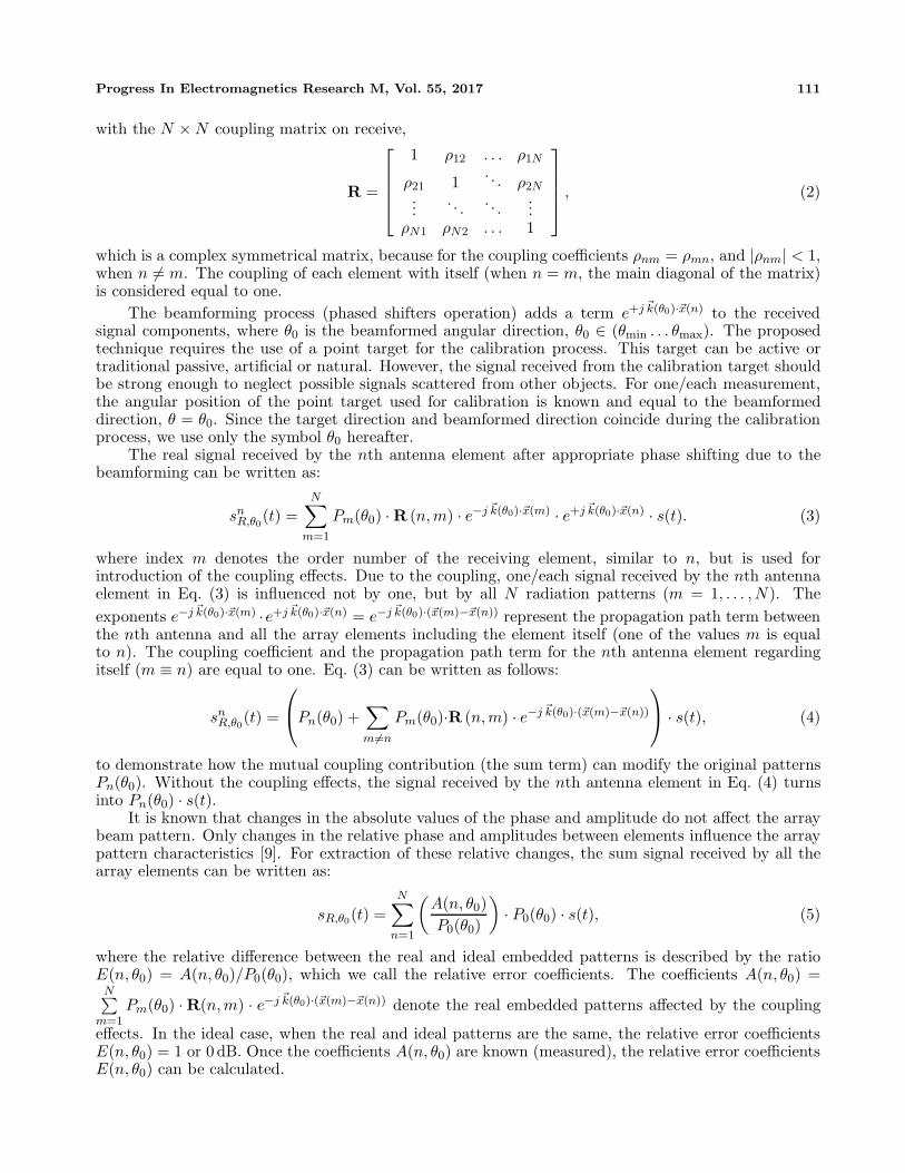
with the N × N coupling matrix on receive,

R =

⎡⎢⎢⎢⎣

1 ρ12 . . . ρ1N

ρ21 1. . . ρ2N

.... . . . . .

...ρN1 ρN2 . . . 1

⎤⎥⎥⎥⎦ , (2)

which is a complex symmetrical matrix, because for the coupling coefficients ρnm = ρmn, and |ρnm| < 1,when n �= m. The coupling of each element with itself (when n = m, the main diagonal of the matrix)is considered equal to one.

The beamforming process (phased shifters operation) adds a term e+j �k(θ0)·�x(n) to the receivedsignal components, where θ0 is the beamformed angular direction, θ0 ∈ (θmin . . . θmax). The proposedtechnique requires the use of a point target for the calibration process. This target can be active ortraditional passive, artificial or natural. However, the signal received from the calibration target shouldbe strong enough to neglect possible signals scattered from other objects. For one/each measurement,the angular position of the point target used for calibration is known and equal to the beamformeddirection, θ = θ0. Since the target direction and beamformed direction coincide during the calibrationprocess, we use only the symbol θ0 hereafter.

The real signal received by the nth antenna element after appropriate phase shifting due to thebeamforming can be written as:

snR,θ0

(t) =N∑

m=1

Pm(θ0) · R (n,m) · e−j �k(θ0)·�x(m) · e+j �k(θ0)·�x(n) · s(t). (3)

where index m denotes the order number of the receiving element, similar to n, but is used forintroduction of the coupling effects. Due to the coupling, one/each signal received by the nth antennaelement in Eq. (3) is influenced not by one, but by all N radiation patterns (m = 1, . . . , N). Theexponents e−j �k(θ0)·�x(m) ·e+j �k(θ0)·�x(n) = e−j �k(θ0)·(�x(m)−�x(n)) represent the propagation path term betweenthe nth antenna and all the array elements including the element itself (one of the values m is equalto n). The coupling coefficient and the propagation path term for the nth antenna element regardingitself (m ≡ n) are equal to one. Eq. (3) can be written as follows:

snR,θ0

(t) =

⎛⎝Pn(θ0) +

∑m�=n

Pm(θ0)·R (n,m) · e−j �k(θ0)·(�x(m)−�x(n))

⎞⎠ · s(t), (4)

to demonstrate how the mutual coupling contribution (the sum term) can modify the original patternsPn(θ0). Without the coupling effects, the signal received by the nth antenna element in Eq. (4) turnsinto Pn(θ0) · s(t).

It is known that changes in the absolute values of the phase and amplitude do not affect the arraybeam pattern. Only changes in the relative phase and amplitudes between elements influence the arraypattern characteristics [9]. For extraction of these relative changes, the sum signal received by all thearray elements can be written as:

sR,θ0(t) =N∑

n=1

(A(n, θ0)P0(θ0)

)· P0(θ0) · s(t), (5)

where the relative difference between the real and ideal embedded patterns is described by the ratioE(n, θ0) = A(n, θ0)/P0(θ0), which we call the relative error coefficients. The coefficients A(n, θ0) =

N∑m=1

Pm(θ0) ·R(n,m) · e−j �k(θ0)·(�x(m)−�x(n)) denote the real embedded patterns affected by the coupling

effects. In the ideal case, when the real and ideal patterns are the same, the relative error coefficientsE(n, θ0) = 1 or 0 dB. Once the coefficients A(n, θ0) are known (measured), the relative error coefficientsE(n, θ0) can be calculated.

112 Babur et al.

3. CALIBRATION TECHNIQUE

3.1. Description

We propose the application of time offsetting to the element wise received signals according tothe circulating signal principle [12]. This principle is known for the possibility of digital transmitbeamforming with the use of only one sounding waveform. With the relative time offset δt introducedinto the received signal components before their summation, the aggregate signal received from thepoint calibration target can be written as follows:

sR,θ0(t) =N∑

n=1

A(n, θ0) · s(t − (n − 1) · δt), (6)

where θ0 is the angular direction of this target, which is known a priori. The ideal (theoretical) radiationpattern of one/each array element P0(θ), contributing to the coefficients A(n, θ0), is supposed to beknown in each considered angular direction θ = θ0.

The introduced time offset δt is inversely proportional to the sounding signal bandwidth ΔF , that isδt = 1/ΔF . This offset also defines the potential range resolution, because, in general, it is equal to themain peak of a signal s(t) after its compression. For waveforms with a large BT-product (compressionratio), the offset components of a signal in Eq. (6) are highly overlapped in time, because the relativetime shift is small compared to the pulse duration Δt � Tp, since Tp = BT × Δt. That is the offsetcomponents of a signal (6) are highly overlapped in time. After their pulse compression, the offsetcomponents become orthogonal in time, because their offset peaks have a width equal to the offset size.The obtained orthogonality exists not depending on the spacing between the array elements.

As known, time or frequency offsetting can affect the radiation pattern of a phased array [13, 14].However, the time offsets introduced in Eq. (6) do not influence the angular-dependent coefficientsA(n, θ0) (real patterns) for the following reason. A phase shift at a given frequency f , associated withthe offset δt, can be written as Δφ = 2π · f · δt. Since the frequency of a sounding signal varies withinΔF , Δφ = 2π. So, the individual time offset δt (or its multiples) applied to the element wise receivedsignals adds the phase shift 2π (or its multiples) not depending on the direction of arrival of the receivedsignals. Therefore, the introduced time delays in Eq. (6) do not affect the estimated coefficients A(n, θ0).

Adding the offsets in the received signal in Eq. (6) allows keeping the same phase relations betweenits components. So, the time shifts in our calibration technique do not influence the radiation pattern,contrary to the approach in [15], where time delays are also used for phased array calibration. Therelative time offset is equal to the width of a compressed signal s(t), that is to the width of the peakof its auto-correlation function ACFs. It means that after pulse compression, the offset componentsof a sum signal can be separated in time domain. In turn, this allows the direct measurement of thecoefficients A(n, θ0) at the output of the pulse compression filter, as shown in Fig. 1.

We assume the pulse compression filter to be matched with the signal s(t). The angular directionis specified as θ0, and the output of the matched filter can be written as:

χθ0(τ) =

∞∫−∞

(N∑

n=1

A(n, θ0) · s(t + τ − (n − 1) · δt))

· s∗(t)dt, (7)

where the superscript ‘*’ means complex conjugation.The matched filter output can be written as

χθ0(τ) =N∑

n=1

A(n, θ0) ·∞∫

−∞s(t + τ − (n − 1) · δt) · s∗(t)dt. (8)

For real signals having a finite length, the integration interval over t is determined by the auto-correlation function of the signal s(t): ACFS , which is non-zero in (−T . . . T ). By expressing theauto-correlation integral in Eq. (8) via the auto-correlation functions of the signal s(t), we obtain:

χθ0(τ) =N∑

n=1

A(n, θ0) · ACFS (τ − (n − 1) · δt). (9)

Progress In Electromagnetics Research M, Vol. 55, 2017 113

The time integral in Eq. (9) results in the offset auto-correlation functions ACFS . For a signals(t) providing good auto-correlation properties (low side-lobes), its normalized discrete ACF can beapproximated as a single sample or a single narrow pulse, ACFS(τ) ∼= δ(τ), where the maximal valueis equal to 1. Therefore, the ACF can provide the filtering properties in time domain by analogy withthe discrete delta function. It is stressed that the approximation on the zero sidelobe level of the ACFis made here for explanation of the calibration method principle that has not been used for modelingor processing of the experimental data presented further in this paper.

We notice that Eq. (9) is not a function of a continuous (can be also discrete) time τ only. It isalso a function of discrete time instants i = n · δt (i = round(τ/δt)). The number of considered timeinstants directly corresponds to the number of receiving elements N . Due to the filtering properties ofthe auto-correlation function, Eq. (9) can be rewritten as:

χθ0(i) =N∑

n=1

A(n, θ0) · δ (i − (n − 1)). (10)

The discrete samples (or pulses) in Eq. (10) are not equal to zero only at specific instants which areseparated in time. Therefore, the estimations of the coefficients A(n, θ0) (the real embedded patternsaffected by the coupling effects) can be measured directly at the output of the matched filter atappropriate time instants i, that is

A(n, θ0) = χθ0(i), for i = n, (11)

where, as we remember, n = 1 . . . N denotes the number of receiving elements, and i = 1 . . . N are theappropriate time samples.

We would like to remind that the real pattern coefficients A(n, θ0) are estimated in the operatingmode, when all N radar channels are functioning, and the corresponding phase shifters specify eachangular direction θ0. It means that the presented calibration technique can take into account a largenumber of effects due to the diffraction, mismatch, variations in elements themselves, etc., which affect

( )s t

0, ( )Rs t

0 0 0 0

0 0 0ˆ ˆ( 1... ) (1, )... ( , ) ,i N A A N

i t t

0

0

1t

2t

(1)

Nt

-

θ

θ=θ

θ θ θ θ

θ

θ θ[ ]θ

==χ

δ=

δ δ

δ

. .

.

Figure 1. Phased array receiver with the introduced time delays.

114 Babur et al.

the embedded patterns Pn(θ0) of the array elements. Therefore, the measured real patterns (coefficientsA(n, θ0)) already include the influence of phase shifters and other effects, such as diffraction.

Based on Eqs. (5) and (11), the correcting (calibration) coefficients for each beamformed angulardirection θ0 can be written as

C(n, θ0) =P0(θ0)

A(n, θ0). (12)

Since a phased array performs beamforming in a number of angular directions, the result of thecalibration procedure in Eq. (12) is shown in the following lookup table having size [N × K]:

C =

⎡⎢⎢⎢⎣

C(1, θ0,1) C(1, θ0,2) . . . C(1, θ0,K)C(2, θ0,1) C(2, θ0,2) . . . C(2, θ0,K)

......

. . ....

C(N, θ0,1) C(N, θ0,2) . . . C(N, θ0,K)

⎤⎥⎥⎥⎦ , (13)

where each column corresponds to one beamformed angular direction θ0,k, k = 1, . . . ,K, where K isan overall number of beamformed directions. During the calibration process, the beamformed angulardirection and the angular position of a calibration target (point scatterer) are equivalent. The calibrationcoefficients are inversely proportional to the relative error coefficients E(n, θ0) = 1/C(n, θ0). Therefore,the relative error matrix E uniquely defines the calibration matrix C and vice versa.

In the operating mode, the signals received by different array elements are not shifted in time.After reception, they are corrected by the appropriate calibration coefficients taken from the lookuptable in Eq. (13) for a given beamformed angular direction θk:

scorrR,θ0,k

(t) =N∑

n=1

C(n, θ0,k)·snR(t), (14)

where the superscript ‘corr ’ stands for ‘corrected’.

3.2. Important Notes

a) The calibration technique can be applied equally well to arrays of any type of radiating elements.The theoretical pattern of an individual array element is supposed to be known.

b) The calibration technique can be applied equally well to equidistant and non-equidistant arrays.This is because the relative time offset δt introduced according to the calibration principle makesthe received signal components orthogonal in time after their pulse compression not depending onthe position vector of the array elements.

c) The calibration method is suitable for small and medium phased arrays. The bandwidth of asounding signal is supposed to be reasonably large. In the case of large phase arrays or smallbandwidth value, the relative time offsets will result in large time delays along the radar channels,which is impractical from an application point of view. It is noted that transmission lines with thegroup velocity smaller than the speed of light can be used for implementation of relatively largetime offsets to the elementwise received signals. Nevertheless, we do not recommend our techniquefor large phase arrays.

d) The calibration method can be easily extended to 2D planar array. It does not require the algorithmmodification. The total number of elements should remain N , and the position vector (see Eq. (1))should describe position of the corresponding 2D array elements. However, the possibility ofpractical implementation of the delays δt, 2 · δt, . . . , (N − 1) · δt significantly limits the use of theproposed method in 2D array applications (N should be reasonably small).

e) The waveform used for calibration and the waveform used for sounding are not necessarily the same.However, they should occupy the same bandwidth and be radiated at the same carrier frequency.The calibration waveform can have any modulation suitable for pulse compression: linear frequencymodulation, phase code manipulation, polyphase coding, etc. It is necessary however to keep inmind that the auto-correlation function (ACF) sidelobes of the waveform used for calibration can,

Progress In Electromagnetics Research M, Vol. 55, 2017 115

in some cases, reduce the accuracy of the extracted calibration coefficients and should be estimatedin advance.

f) The introduced time delays can affect the signals during the calibration process. Their influencecan be estimated by using the proposed calibration technique when the delays are switched on,and the array is switched off (the sounding signal is sent directly to the receiver channels). Thedistortion coefficients introduced by the delay lines can be estimated as the amplitude of the signalsat the matched filter output for one received pulse.

4. VALIDATION OF THE PROPOSED CALIBRATION TECHNIQUE

The proposed calibration technique has been validated using a fully digital array test-bed in its operatingmode. The receiving linear phased array is made of N = 8 antennas (patches) spaced by a half-wavelength distance d = λ/2 from each other. The carrier frequency was equal to 10 GHz. The down-converted signals were digitized and processed. The digit capacity of the analog-to-digital converter wasequal to 14 bit. The sampling rate was equal to 125 MHz. The experimental results are presented for asounding LFM signal. The pulse duration and bandwidth were equal to 320 µs and 40 MHz, respectively.The measurements were carried out by using an active radiator (as a point scatterer) in the far field ofthe array. The experiment was performed in the anechoic chamber. No window weighting was appliedto the received signals. The ideal embedded pattern P0(θ) of each array element was described by acosine function.

The phases of the digitized received signals were initially changed appropriately for each angulardirection of the calibration target θ0. Then the digitized signals were summed with appropriate offsets(n − 1) · δt, where n is a number of the receiving channel, n = 1 . . . 8. It is equivalent to the properanalog summation described by Eq. (6). The smallest and largest offsets were equal to 25 ns and 175 ns(equivalent to 7.5 m and 52.2 m), respectively. Since the total delay length is rather large, compacttransmission lines are advised to be used for practical implementation of our example. The calibrationcoefficients in Eq. (12) were extracted from the sum signal at the matched filter output (see Fig. 1).After that, the phase and amplitude correction coefficients were applied to the original received signals.One received pulse was used during the calibration technique for each considered angular direction θ0

within the angular sector [−40◦ . . . + 40◦] with a step of 5◦.Figure 2 visualizes the normalized matched filter output (thick black line) for one given angular

direction, the components of the output signal (thin colored lines) and the characteristic points (8black dots) show the estimated coefficients A(n, θ0) used for calculation of the calibration coefficientsby Eq. (12). It is stressed that the characteristic points coincide in time with the zeros of the sidelobesof the interfering components (see the colored lines). Therefore, in our example, the relatively highsidelobes do not affect the estimation of the coefficients A(n, θ0).

The calibration procedure provides the calibration coefficients C(n, θ0) and the relative errorcoefficients E(n, θ0), which uniquely define each other. The amplitude and phase of the relative errormatrix E is shown in Figs. 3(a)–(b), respectively. The edge effects affect the first and last array elements,where the error amplitudes are higher (Fig. 3(a)). In turn, the phase distortions are higher for the innerelements of the array (Fig. 3(b)). Nevertheless, Fig. 3 proves that the amplitude and phase errors canbe evaluated for each given beamformed direction. When evaluated, the errors can be compensatedafterwards.

Figure 4 shows the array patterns (functions of the observed angular direction θ) for a number ofbeamformed directions θ0 in comparison with the corresponding array factors (black lines). The realarray patterns (red lines) before the calibration are reported in Fig. 4(a). The red lines in Fig. 4(b)show the calibrated array patterns after compensation of the phase and amplitude errors. The idealradiation pattern P0(θ) of the individual antenna element (in gray) is represented as the envelope of thearray patterns in Fig. 4. A closer inspection of the figures allows the detection of the difference betweenthe non-calibrated and calibrated data.

Figure 5 shows the difference between the real and ideal array patterns as functions of an observedangular direction θ calculated for all the beamformed angular directions θ′ ∈ [−40◦, . . . , 40◦] with astep of 5◦. The real array patterns are measured. The ideal (theoretical) array patterns are calculatedunder ideal conditions: in the absence of coupling and parasitic effects, with no difference between

116 Babur et al.

the embedded patterns of the elements, etc. In Fig. 5(a), the average deviation is −37.4 dB for−90◦ < θ < 90◦ (all possible angles) and −38.7 dB for −50◦ < θ < 50◦ (within the −3 dB beamwidth ofthe individual array element, see Fig. 4). The average deviation in Fig. 5(b), when the phase errors arecompensated, is −40.1 dB within −90◦ < θ < 90◦ and −40.7 dB within −50◦ < θ < 50◦. After amplitudecompensation, the average deviation values (see Fig. 5(c)) are −41.0 dB and −41.3 dB, respectively. Inour example, the amplitude correction is slightly more effective than phase correction. When bothamplitude and phase corrections are applied (see Fig. 5(d)), the deviation from the ideal pattern iscompletely compensated, error levels being below the considered minimal threshold of −50 dB.

We want to stress that the amplitude and phase corrections in our radar test-bed have beenimplemented by the signal processing means on the received digitized signals. In reality, the

Figure 2. The matched filter output for one given angle (thick black line), its components (thin colorlines) and the measured values (8 black dots).

0(deg)

n n

Amplitude of Error Matrix (dB) Phase of Error Matrix (rad)

0(deg)θ θ

(a) (b)

Figure 3. The relative error matrix E: (a) modulus of the amplitude (dB), (b) phase (rad).

Progress In Electromagnetics Research M, Vol. 55, 2017 117

compensation of phase and amplitude errors has to be implemented via phase shifters and attenuatorsintegrated in the system. The proposed calibration technique takes into account static and dynamicerrors, because it is executed during the operating mode of the radar. However, the quantization noiseof the phase and amplitude control unit cannot be compensated, thereby limits the accuracy of theproposed calibration technique.

5. CONCLUSION

This paper presents a novel simple calibration technique applicable to radars with small- or medium-sizephased arrays. Calibration challenges in radar technology are outlined. Solutions based on the proposedtechnique are proposed and validated by using a radar with an 8-element linear antenna array. Thefactors limiting the accuracy of the proposed calibration technique are described and analyzed.

The presented calibration technique is implemented directly during the operating mode of a phasedarray radar, and thanks to that, can efficiently account for a large number of parasitic effects such asmutual coupling between array elements, diffraction phenomena, mismatch, and performance variationsat antenna level. As a matter of fact, the developed technique relies on the application of a suitable timeoffsetting in combination with a switching control between calibration and normal operation of the radarsystem. Furthermore, the proposed calibration methodology does not require direct measurement of theantenna characteristics or use of matched loading on the array elements. The real embedded patternsof the array elements and mutual coupling effects are taken into account by angular-dependent errorcoefficients which are derived during the calibration process. The drawback of the proposed calibrationtechnique is that it is not suitable for large arrays, because the implementation of the introduced timeoffsets is limited from the practical point of view.

Finally, it is stressed that even in case the presented calibration scheme cannot be executed in acontrolled laboratory environment, its implementation on the field is still possible by using one dominantpoint target.

ACKNOWLEDGMENT

This work was carried out in the framework of the project 8.909.2014/K funded by the Ministry ofEducation and Science of the Russian Federation.

Non-calibrated Array Patterns Calibrated Array Patterns

(deg)θ (deg)θ

(a) (b)

Figure 4. (a) Non-calibrated and (b) calibrated array patterns (in red) in comparison with the arrayfactors (in black); the individual element pattern(in gray), normalized.

118 Babur et al.

0θ (deg)

Before Calibration After Calibration (phase only)

0θ (deg)

(deg)

θ

(deg)

θ

After Calibration (amplitude only) After Calibration (phase&amplitude)

0θ (deg)0θ (deg)

(deg)

θ

(deg)

θ

(a) (b)

(c) (d)

Figure 5. Difference between the real and ideal (theoretical) array patterns (a) before calibration,(b) after phase correction, (c) after amplitude correction and (d) after amplitude and phase correction,(absolute value).

REFERENCES

1. Mailloux, R. J., Phased Array Antenna Handbook, 2nd Edition, Artech House, Inc., Norwood, MA,2005.

2. Hansen, R. C., Phased Array Antennas, John Wiley & Sons, Inc., New York, 2009.3. Caratelli, D. and M. C. Vigano, “Analytical synthesis technique for linear uniform-amplitude sparse

arrays,” Radio Science, Vol. 46, No. 4, RS4001, Aug. 2011.4. Caratelli, D. and M. C. Vigano, “A novel deterministic synthesis technique for constrained sparse

array design problems,” IEEE Transactions on Antennas and Propagation, Vol. 59, No. 11, 4085–4093, Nov. 2011.

5. Gupta, I. J. and A. K. Ksienski, “Effect of mutual coupling on the performance of adaptive arrays,”IEEE Transactions on Antennas and Propagation, Vol. 31, 785–791, May 1983.

6. Babur, G., P. Aubry, and F. Le Chevalier, “Antenna coupling effects for space-time radarwaveforms: analysis and calibration,” IEEE Transactions on Antennas and Propagation, Vol. 62,No. 5, 2572–2586, 2014.

7. Tyler, N., B. Allen, and H. Aghvami, “Adaptive antennas: The calibration problem,” IEEECommun. Mag., Vol. 42, No. 12, 114–122, 2004.

8. Sorace, R., “Phased array calibration,” IEEE Transactions on Antennas and Propagation, Vol. 49,

Progress In Electromagnetics Research M, Vol. 55, 2017 119

No. 4, 517–525, 2001.9. Tsoulos, G. and M. Beach, “Calibration and linearity issues for and adaptive antenna system,”

IEEE Vehicular Tech. Conf., Vol. 3, 1596–1600, May 1997.10. Seker, I., “Calibration methods for phased array radars,” Proc. of SPIE, Vol. 8714, 2013, Available

at: http://proceedings.spiedigitallibrary.org/ on 09/08/2013.11. Huang, Z. and C. A. Balanis, “Mutual coupling compensation in UCAs: Simulations and

experiement,” IEEE Transactions on Antennas and Propagation, Vol. 54, 3082–3086, Nov. 2006.12. Babur, G., P. Aubry, and F. Le Chevalier, “Space-time radar waveforms: Circulating codes,”

Journal of Electrical and Computer Engineering, Vol. 2013, Article ID 809691, 8 pages, 2013.13. Antonik, P., M. C. Wicks, H. D. Griffiths, et al., “Frequency diverse array radars,” Proc. IEEE

Radar Conf. Dig., 215–217, Verona, NY, USA, 2006.14. Longbrake, M., “True time-delay beamsteering for radar,” Proc. of the IEEE National Aerospace

and Electronics Conference (NAECON ’12), 246–249, Dayton, USA, 2012.15. Alfred, Q. M., T. Chakravarty, and S. K. Sanyal, “A novel schematic for calibration of large phased

array antenna using programmable time-delay units,” Progress In Electromagnetics Research,Vol. 65, 81–91, 2006.