From%banks’%strategies%to%financial%(in)stability

Simone%Berardi%Gabriele%Tedeschi%

2015%/%11%

!

From banks’ strategies to financial (in)stability

2015 / 11 Abstract

This paper aims to shed light on the emergence of systemic risk in credit systems. By developing an interbank market with heterogeneous financial institutions granting loans on different network structures, we investigate what market architecture is more resilient to liquidity shocks and how the risk spreads over the modeled system. In our model, credit linkages evolve endogenously via a fitness measure based on different banks’ strategies. Each financial institution, in fact, applies a strategy based on a low interest rate, a high supply of liquidity or a combination of them. Interestingly, the choice of the strategy influences both the banks’ performance and the network topology. In this way, we are able to identify the most effective tactics adapt to contain contagion and the corresponding network topology. Our analysis shows that, when financial institutions combine the two strategies, the interbank network does not condense and this generates the most efficient scenario in case of shocks.

Keywords: Interbank market, dynamic network, fitness model, network resilience, bank strategy JEL classification: G01, G02, D85

Simone Berardi Universitat Jaume I

Department of Economics berardi@uji.es

Gabriele Tedeschi UJI & Universita Politecnica delle Marche

Dipartimento di Scienze Economiche e Sociali gabriele.tedeschi@gmail.com

From banks’ strategies to financial (in)stability

Simone Berardi

⇤and Gabriele Tedeschi

⇤,⇤⇤

* Universitat Jaume I. ** Universita Politecnica delle Marche, Ancona.

E-mail: berardi@uji.es; gabriele.tedeschi@gmail.com

August 3, 2015

Abstract

This paper aims to shed light on the emergence of systemic risk incredit systems. By developing an interbank market with heterogeneousfinancial institutions granting loans on di↵erent network structures,we investigate what market architecture is more resilient to liquidityshocks and how the risk spreads over the modeled system. In ourmodel, credit linkages evolve endogenously via a fitness measure basedon di↵erent banks’ strategies. Each financial institution, in fact, ap-plies a strategy based on a low interest rate, a high supply of liquidityor a combination of them. Interestingly, the choice of the strategyinfluences both the banks’ performance and the network topology. Inthis way, we are able to identify the most e↵ective tactics adapt tocontain contagion and the corresponding network topology. Our anal-ysis shows that, when financial institutions combine the two strategies,the interbank network does not condense and this generates the moste�cient scenario in case of shocks.JEL codes: G01; G02; D85

Keywords: Interbank market; dynamic network; fitness model;

network resilience; bank strategy.

1 Introduction

The role of the financial sector and the e↵ects of financial developmenton the economic system have been extensively debated (Schumpeter 1911;Robinson 1952). Specifically, the development of the financial sector has tra-ditionally been indicated as a key ingredient of the economic growth (Rajanand Zingales 1998; Levine 2005), as an instrument to foster entrepreneur-ship (Black and Strahan 2002) and increase firms’ productivity (Herreraand Minetti 2007, Dabla Norris et al. 2012). However, recent evidencehas suggested that the rapid flourishing of the finance industry could havea negative e↵ect on the economic system (Arcand et al. 2011). The fastexpansion of the financial sector in the last decades, therefore, has been

1

associated with an increased economic instability and fragility and with ahigher systemic vulnerability (Wray 2009; Tridico 2012). In this respect,the European Central Bank (ECB) itself is worried about the fact the toolscurrently available to monitor financial systems are insu�cient (see Trichet2010). Such inadequacy is also among the major concerns of the EuropeanCommission, which has just created the European Systemic Risk Board.A general discontent over the ability of our current theoretical frameworksto fully understand economic systems and evaluate their systemic propertieshas led scholars to analyze them in a dynamic way. Specifically, the presentsituation is ripe for a change of approach. ECB has called o�cially for (1)more integrated systems, (2) a systemic approach that takes into accountthe network of financial exposures, and (3) new appropriate systemic riskindicators (Issing 2009).Following this line of thought, in this paper, we present a stylized interbankmarket and analyze the endogenous source of instability in the credit system.By combining network theory and heterogeneous agents approach we inves-tigate, in an evolutionary framework, the dynamics which are detrimental tothe financial stability. Specifically, we emphasize the e↵ect of di↵erent banks’strategies and di↵erent network architectures on the resiliency and robust-ness of the credit system. Indeed, as the economic literature on contagionhas highlighted, the financial market structure and its interconnectednessare key ingredients to explain systemic failure propagation. The commonidea is that two opposite e↵ects interact in credit networks: the risk sharing,which decreases with the network connectivity and the systemic risk that,in contrast, increases with linkages (see, for instance, Allen and Gale 2000,Thurner et al. 2003, Iori et al. 2006, Battiston et al. 2007, Battiston et al.2012a,b, Tedeschi et al. 2012).In confirmation of the results of many of the above mentioned studies, thiswork shows that the relationship between connectivity and systemic riskis not linear but involves di↵erent forces. Specifically, agents’ heterogeneityand their financial fragility seem to be a leading force in generating propaga-tion of systematic failure. On the one hand, in fact, the possible emergenceof contagion depends crucially on the degree of heterogeneity. Indeed, whenthe agents’ balance sheets are heterogeneous, banks are not uniformly ex-posed to their counter-party. Therefore, if contagion is triggered by thefailure of a big bank, which represents the highest source of exposure for itscreditors, the situation is certainly worse than when agents are homogeneous(see Iori et al. 2006; Caccioli et al. 2012; Lenzu and Tedeschi 2012; Tedeschiet al. 2012). On the other hand, the probability of default in credit marketsis strictly linked to the presence of highly leveraged agents. Indeed, whenvariations in the level of financial robustness of institutions tend to persistin time or to get amplified, financial linkages among financially fragile banksrepresent a propagation channel for contagion and a source of systemic risk(see Lorenz and Battiston 2008; Battiston et al. 2012a). Moreover, our

2

analysis shows that another force plays a crucial role in causing financialdistress, namely the interest rate. When a lender accords a loan to an over-leveraged agent it applies, via the financial accelerator (see Bernanke andGertler 1989, 1990; Grilli et al. 2014,a,b) higher interest rate. This, in turn,worsens the financial condition of the borrower itself pushing it towards thebankruptcy state. If one or more borrowers are not able to pay back theirloans even the lenders’ equity is a↵ected by bad debts. Therefore, lendersreduce their credit supply and increase the borrowers’ rationing. In this way,the profit margin of borrowers decreases and a new round of failures mayoccur.The problems arising from financial market interconnectedness have alsobeen highlighted by empirical studies, which have analyzed the propertiesof credit networks during di↵erent phases of the economic cycle (Cocco etal. 2009; Hale 2011; Schiavo et al 2010; Minoiu and Reyes 2011; Chinazzi etal. 2012; Memmel and Sachs 2013; Tonzar 2015) and defined new analyticaltools able to better identify and monitor systemic risk and crisis transmis-sion (Sornette and Von der Becke 2011; Kaushik and Battiston 2012; Catulloet al. 2015).

The originality of this work in respect to previous mentioned models oninterbank networks is in the credit linkages evolution. In our frameworkfinancial connections might change over time via a preferential attachmentevolving procedure (see Barabasi and Albert 1999; Tedeschi et al. 2014;Grilli et al. 2015) such that each financial institution can enter into a lendingrelationship with others with a probability proportional to a fitness measure.Specifically, we implement a compound fitness parameter, which is a combi-nation between banks’ supply of liquidity and their interest rate. Banks canattract their customers by o↵ering a higher supply of liquidity or a lowerinterest rate. Our financial institutions, modeled as risk neutral agents oper-ating in a perfect competition environment, maximize their expected profitsand, consequently, set their optimal interest rate. The optimization mecha-nism is designed such that the bigger banks (i.e the more liquid ones) o↵erhigher interest rates while the smaller ones (i.e the less liquid ones) seek toattract customers by setting cheaper interest rates. From the point of viewof the borrowing banks, knocking on the door of a big financial institutionguarantees the loan satisfaction but at a high financing cost. Otherwise,knocking on the door of a small institution increases the chance of creditrationing but reduces financing costs. The fitness parameter, therefore, notonly identifies di↵erent banks’ strategies, but also behaviors that endoge-nously evolve on the base of the agents’ size. Moreover, this method, basedon a compound fitness parameter given by two di↵erent banks’ strategies,is able to reproduce di↵erent network topologies ranging from the randomgraph to the scale-free one.In each time period, we perturb the system with random liquidity shocks,

3

arising ultimately from the deposit and withdrawal patterns of customers.Since liquidity fluctuations are unpredictable, a bank may find itself unableto meet payment obligations due to the illiquidity of its available assets.If no interbank market is present, the mere inability to meet customer de-mands triggers o↵ failure. If interbank lending is possible, an illiquid bankmight seek funds not just to make payments but also to repay past creditors.If despite such e↵orts, a bank ends up with insu�cient funds, we assume forthe sake of simplicity that it too closes down.An important di↵erence distinguishes our “failure mechanism” from thosecommonly used in physical and economic literature (see, for instance, Bat-tiston et al. 2012a; Albert et al. 2000). All these models generate anexogenous random (or targeted) attack and study the consequences of re-moving a hit vertex on nodes connected to it and on the network structure.In line with these studies, we generate a random attack via a liquidity shockbut, di↵erently from them, not necessarily the hit node is removed. Thefailure depends endogenously from node’s capacity to rise liquidity in theinterbank market and, lastly, from the network topology.

Our work is closely related to Lenzu and Tedeschi 2012 (LT hereinafter).In their paper, the authors consider an interbank network where credit link-ages evolve via a fitness parameter given by banks’ expected profit. Bychanging the signal credibility that agents attribute to the counter-partyperformance (i.e the expected profit) the interbank network evolves throughdi↵erent architectures. Specifically, low values of the signal credibility char-acterize random graphs with a Binomial (or Poisson) in-degree distribution,exponential and scale-free topologies emerge for intermediate values of theparameter, while the market self-organizes into a pseudo-star for higher val-ues of the signal. By perturbing the system with liquidity shocks, the authorstest the network capacity to flow liquidity and its resilience. The authorsfind that even though random networks are characterized by a low credibil-ity signal, they are more e�cient in re-allocating liquidity from banks thathave a surplus to the banks that have a shortage. Instead, as the networkbecomes scale-free with the increase in the credibility signal, banks becomemore prone to failure due to illiquidity. In particular, there would be just asmall number of highly trusted agents, leaving all others with very few creditlines and hence being more exposed in case of negative liquidity shocks.As in LT, we amplify our fitness measure with a multiplicative parameterwhich represent the signal on banks’ attractiveness and shapes the inter-bank network topology. On the one hand, when the signal is high, theagents’ behavior is characterized by “herding”, a phenomenon which occursin situations with high information externalities, when agents’ private in-formation is swamped by the information derived from directly observingothers actions. In this circumstance, few lenders gain the lion’s share ofborrowers, attracting a high percentage of in-coming links at the expense

4

of many feebly connected ones. On the other hand, when the signal is low,agents “shop around”, the network does not condensed and the credit ismore uniformly distributed in the system.A significant di↵erence characterizes the evolution of our interbank net-work with respect to that of LT. We implement di↵erent banks’ strategieswhich compete with each other. These strategies that parametrize the fit-ness measure not only generate competition among banks, but also modifyendogenously the interbank network topology. In this circumstance, whenwe modify the “signal credibility”, we are not only able to investigate howdi↵erent banks’ strategies perform in di↵erent network architectures, butalso to estimate the impact that these strategies have in generating di↵erentnetwork topologies.Another relevant di↵erence between this model and that of LT is the banks’balance-sheet structure. The LT interbank market is a zero-liquidity system,meaning that at the beginning and at the end of each period, banks hold noliquidity. The liquidity, thus, is exogenously generated as positive shocks af-fecting financial institutions. Specifically, each time period only two randombanks receive a liquidity shock of equal magnitude but opposite sign. Thebank receiving the negative shock becomes potential borrower, while thebank hits by the positive shock become potential lender. All other interme-diate nodes act as liquidity conduits, receiving and forwarding funds. Thisassumption allows authors to define a flow network and solve the maximum-flow problem by using the simple Ford-Fulkerson method. The use of an in-terbank flow network allow the authors to analytically determine the liquid-ity flow between any pair of banks in the market (see Ford-Fulkerson 1956;1962). However assuming a zero-liquidity system means not to consider therepayment mechanism between borrower and lender. In this work we re-lax this hypothesis. Specifically, we apply multiple liquidity shocks on thebank deposit motion (not bilateral as in LT) and model a repayment mech-anism between lenders and borrowers. The repayment mechanism, whichrequires banks to repay installment and interest, has two important conse-quences. First, it allows us to define a micro-founded interest rate, whereasthis is constant in LT. Second, it generates a more interesting dynamic in theagents’ failure. In fact, in the LT model bankruptcies depend exogenouslyon the random attack and endogenously on borrower’s capacity to rise liq-uidity in several interbank network topologies (see, for instance, Lee 2013).In this model we extend the two bankruptcy mechanisms presented in LTby adding a third one based on the repayment scheme. Specifically, the re-payment mechanism can trigger an additional channel of failures. Startingfrom the failure of a borrowing financial institution, this mechanism has anegative feedback on the lender balance-sheet via bad debt. If the shock isbig enough to completely erode the bank net-worth, then the lender itselfwill fail. Otherwise, if the shock does not fully corrode the lender equity,then the bank survives. However, in this circumstance, the “weakened” fi-

5

nancial institution will attempt to recover losses or by raising interest ratesor decreasing the supply of liquidity. In both cases, this attitude will furtherweaken the borrowing banks with the result, therefore, of causing additionalbankruptcies.

The rest of the paper is organized as follows. In Section 2 we describethe model by analyzing the dynamic of the interbank network as well as thefunctioning of the trading mechanism on the interbank system. In Section3 we present the results of the simulations. Specifically, we proceed in twosteps: firstly, we provide a general overview of the credit network dynamicsby varying the credibility signal and banks’ strategies; secondly, we studythe impact of the di↵erent network topologies on contagion phases. Finally,Section 4 concludes.

2 The model

2.1 The interbank credit relationships: a dynamic network

approach

We start the description of the model by explaining formation and evolu-tion of the interbank network. In our network, nodes represent banks andedges are the connective links between them. Links are directional, they arecreated and deleted by banks who look for credit and point to the financialinstitution that grants loan.

In general local interaction models agents interact directly with a finitenumber of others in the population, the so-called “neighbors”. In our modelthe number of out-going links is constrained to be d, thus borrowing bankscan only get loan from few lenders. There are two important reasons behindit. On the one hand, in a highly connected random network, synchroniza-tion could be achieved via indirect links. The impact of direct credit linkson the systemic risk is easier to be tested in a diluted network where indi-rect synchronization is less likely to arise. On the other hand, by keeping afixed connectivity, we can easily compare the performance of di↵erent mar-ket topologies to spread liquidity through the network.

At any time t, the banking system is populated by N banks belongingto the finite set ⌦t = i, j, k, .... Financial institutions are interconnected bycredit relationships represented by the set N t, whose elements are orderedpairs of distinct banks. Banks (nodes or vertices) and their financial rela-tionships (edges or links) form the financial network Gt(⌦t

,N t).

We implement an endogenous mechanism of preferential attachmentbased on a compound fitness parameter. Specifically, we implement a fitness

6

function which is a linear combination between the bank liquidity and itsinterest rate. Banks start with identical initial conditions, so that all agentshave the same initial liquidity and interest rate. As time goes by, some fi-nancial institutions may become more liquid than others or o↵er rates lowerthan their competitors. As a measure of the agent attractiveness we definethe fitness at time t as a combination between the bank liquidity relative tothe liquidity ⌅t

max

of the most liquid agent imax

and its interest rate relativeto that rt

min

of the cheapest financial institution:

�

t

i

= ✏

✓⌅t

i

⌅t

max

◆+ (1� ✏)

✓r

t

min

r

t

i

◆. (1)

✏ measures the weight that the bank gives to the liquidity or to the interestrate. When ✏ is equal to zero, the bank strategy is in o↵ering low rateswhile, when ✏ is equal to one, the strategy consists in providing high liquiditysupply.The bank’s liquidity, ⌅t

i

, in Eq. (1) comes from the inter-day bank balance-sheet:

C

t

i

+ L

t

i

= D

t

i

+ E

t

i

, (2)

with assets (i.e cash, Ct

i

, and long term assets, Lt

i

) on the left hand sideof the identity and liabilities (i.e deposits, Dt

i

, and equity, Et

i

) on the righthand side. In our simple framework, the liquidity, which corresponds tothe supply of liquidity, ⌅t

i

, is the 98% of the bank cash. It implies that, asrequired by Basel III, the bank has to hold an amount of 2% of its cash asa capital reserve.The interest rate, rt

i

, in Eq.(1) comes from the expected profit of a loan fromthe lender1 i to the borrower j:

E[⇧t

i,j

] = (1� p

t

j

)rti,j

c

t

i,j

+ p

t

j

(↵At

j

� c

t

i,j

) + �A

t

j

� �A

t

i

. (3)

The parameters in the Eq. (3) should be interpreted as follows: p

t

j

is theborrower’s default probability, ct

i,j

is the maximum amount bank i is willingto lend to j, ↵ is the liquidation cost of assets pledged as collateral, At

j

theagent j’s assets and, � and �, are lender’s screening cost of establishing alink2. The first term on the right hand side of Eq.(3) shows the expectedrevenue if the borrower repays its obligation, the second term the expectedrevenue in case of the borrower’s default (in this case borrower’s collateral issold) and the last two terms are the opportunity costs of the agreement. By

1We identify with the index i a generic bank or a lending bank. The index j, otherwise,

identifies a borrowing bank.

2The screening cost decreases with the dimension of the borrower’s assets and increases

with the lender dimension (see, for example, Berger et al. 2001; Dell’Ariccia & Marquez

2004; Maudos et al. 2004).

7

imposing Eq.(3) equal to zero and solving it for rti,j

, we obtain the interbank

interest rate ensuring zero expected profits3:

r

t

i,j

=�A

t

i

� �A

t

j

� p

t

j

(↵At

j

� c

t

i,j

)

(1� p

t

j

)cti,j

. (4)

The interest rate asked by the lender i to the borrower j increases withthe lender’s size (i.e its assets) and the borrower’s financial fragility. Inother words, we assume that the interest rate charged by lenders embodiesan external finance premium increasing with the leverage, and, therefore,inversely related to the borrower’s net worth4. In our model, therefore, thebank behaves as a lender in a Bernanke and Gertler (1989, 1990) worldcharacterized by asymmetric information and costly state verification (seeBernanke, Gertler, and Gilchrist (1999) for a comprehensive exposition ofthe approach).Moreover, the interest rate in Eq.(4) is not linearly related to the bank’sprobability of default pt

j

, and its capacity c

t

i,j

. The probability of default ofthe borrower j is given by:

p

t

j

=

1�

E

t

j

E

t

max

!. (5)

Following Greenwald & Stiglitz 1993, our financial institutions go bankruptwhen their equity at time t becomes negative, E

t

j

< 0. We implementa simple probability of bankruptcy in line with this idea: the higher thedistance between the equity of bank j with respect to that of bank with thehighest equity, the higher its default probability.The lending capacity, ct

i,j

, in Eq.4, representing the maximum amount lenderi is willing to lend to j, is given by:

• c

t

i,j

= (1� h

t

j

)At

j

> 0 if (i, j) 2 N t

• c

t

i,j

= 0 otherwise

where A

j

are the assets pledged by borrower j to lender i as collateraland h

j

2 (0, hmax

] is the borrower haircut. We define the haircut as

h

t

j

=⇣

�

t

j

�

t

max

⌘, with �

t

j

=L

t

j

E

t

j

to be the agent’s leverage.

3We assume that banks are risk neutral agents operating in a perfect competition

environment.

4This assumption comes from the balance sheet identity (see Eq. 2), where we observe

that the interest rate asked by the lender is a positive function of the borrower’s leverage,

�, and a negative function of the lender’s leverage: in fact At

i

=

L

ti

�

ti+Dt

i

, with �t

i

=

L

ti

E

ti.

8

Each borrowing bank j starts with some outgoing link with some randomagents (i.e borrowing position), and possibly with some incoming links fromother agents (i.e lending position). Links are rewired at the beginning of eachperiod, in the following way: each financial institution j cuts its outgoinglink, with agent i, and forms a new link, with a randomly chosen agent k,with a probability

Pr

t

j

=1

1 + e

��(�t

k

��

t

i

)(6)

or keep its existing link with probability 1 � Pr

t

j

. Thus, the probabilitythat a link exists between a pair of banks is equal to the fitted probabilityfrom the logit regression (Vandenbossche et al. 2013; Tedeschi et al. 2012and Tedeschi et al. 2014). The parameter � 2 [0,1] in Eq. 6 is the keyelement generating di↵erent network structures. It represents the “inten-sity of choice” and answers the question on how much financial institutionstrust the information about other agents’ performance. For 0 < � < 1di↵erences in fitness are smoothed, unchanged for � = 1 and amplified for� > 1 (Domencich et al. 1975; Lenzu and Tedeschi 2012). The algorithm isdesigned so that successful banks gain a higher number of incoming links.Nonetheless, the algorithm introduces a certain amount of randomness, andlinks to more successful banks have a finite probability to be cut in favorof links to less successful banks. In this way, we model imperfect informa-tion and bounded rationality. At the same time, the randomness also helpsunlock the system from the situation where all agents link to the same bank.

2.2 A stylized interbank trading mechanism

Each time period t, banks face deposit motions which modify their inter-daybalance-sheet (see Eq.2). Deposits evolve as follows:

D

t

i

= D

t�1i

(1 + ⌘u

t

i

), (7)

where ⌘ is a constant and u

t

i

⇠ N (0, 1) is a normal noise.On the one hand, banks running into a deposit reduction and, with in-su�cient liquidity to meet the withdrawal, enter the interbank market asborrowers. On the other hand, banks facing a deposit increment and, con-sequently, a liquidity increase, enter the interbank market as lenders. Thebank i debt or credit positions in the interbank market are given by:

• borrower if �D

t

i

+ ⌅t

i

0, with demand of liquidity d

t

i

= |�D

t

i

+ ⌅t

i

|,

• lender if �D

t

i

+ ⌅t

i

> 0, with supply of liquidity s

t

i

= �D

t

i

+ ⌅t

i

,

with �D

t

i

to be the deposit variation between before and after the shock.In our model, thus, liquidity shocks trigger the interbank market. Liq-uid financial institutions become potential lenders, while illiquid banks can

9

try to borrow from financial institutions they have previously entered intoagreements with. Banks hit by the negative shock, thus, can raise fundsby exploiting their lending agreements and, when the gathered loan is notenough to fully fulfill their liquidity need, by selling their long term assets, Lt

i

(see Eq.2). Given the long maturity of bank assets, we assume that banksconsider the asset sale as a second-best choice which occurs at extremelydiscounted prices. Specifically, we define the granted loan from lender, i,to borrower, j, as: l

t

i,j

= min(sti

, d

t

j

). The borrowing bank finding, via theinterbank market, enough loan to cope with the shock can deal with with-drawals. On the contrary, the rationed bank j (i.e d

t

j

> s

t

i

) has to sell an

amount of its long term asset equal to d

t

j

� s

t

i

= ⇢L

t

j

, where ⇢ is the ’fire-

sale’ price and L

t

j

the amount of loan, Lt

j

, bank j has to sell for covering itsresidual liquidity need.

At the beginning of the next day, the repayment round takes place.Banks run into a new deposit motion (see Eq. 7) increasing or decreasingtheir liquidity. On one hand, lending banks facing a positive variationof deposits (i.e �D

t

i

� 0), increase their cash and, consequently, remainpotential lenders. Otherwise, if they face a negative variation of deposits (i.e�D

t

i

< 0), they become borrowers. On the other hand, borrowing banks

addressing a positive variation of deposits can fully repay their previousloan if �D

t

j

� l

t�1i,j

(1 + r

t�1i,j

)). Otherwise, if �D

t

j

< l

t�1i,j

(1 + r

t�1i,j

), theyhave to sell their long term assets in order to repay creditors. The amountof long term assets sold by j is: ⇢L

t

j

= l

t�1i,j

(1 + r

t�1i,j

), with l

t�1i,j

to be theamount of interbank loan the borrower j has still to meet with. Borrowingbanks addressing a negative variation of deposits have to sell their long termassets in order to pay their previous interbank loan and address the newliquidity needs. In this circumstance, the amount of asset sold is: ⇢L

t

j

=

l

t�1i,j

(1 + r

t�1i,j

) + �D

t

j

.5 Banks unable to fully fulfill their liquidity needdefault. Bankrupt agents’ assets are liquidated in the claimants’ favor. Inthis case, involved lenders incur a credit loss (i.e bad debt) equal to B

t

i,j

=(1�↵�h

t

j

)At

j

, net of the collateral liquidation value. Borrowing and lendingfinancial institutions absorb, with their equity, the ‘fire-sale’ and bad debtlosses. The generic bank i net worth evolves according to:

E

t

i

= E

t�1i

+X

j

r

t�1i,j

l

t�1i,j

�X

j2⇥t

i

B

t

i,j

� (1� ⇢)Lt

i

, (8)

where ⇥t

i

is the subset of the bank i clients unable to pay their debts backbecause they go bankrupt. Financial institutions go bankrupt when theirequity at time t becomes negative, E

t

i

< 0. The failed banks leave the

5For the sake of simplicity, we assume that banks can not renegotiate their debt posi-

tion, but should extinguish it by the day.

10

market. When banks fail, they are replaced by new entrants, which are onaverage smaller than incumbents. So, entrants’ size is drawn from a uniformdistribution centered around the mode of the size distribution of incumbentbanks (see Bartelsman et al. 2005).

3 Simulation results

We consider an economy consisting of N = 100 banks over a time span ofT = 1000 periods. Each bank is initially endowed with the same balance-sheet: C0 = 30, L0 = 120, D0 = 135 and E

0 = 15. Three are the parametersentering into the interest rate. Specifically, we fix: � = 0.05, � = 0.02 and↵ = 0.3.We fix the number of out-going links, d = 1, and the constant parameter inEq. 7, ⌘ = 0.035. The robustness of our qualitative results has been checkedby employing Monte Carlo techniques. We have run 100 independent simu-lations for di↵erent values of the initial seed generating the pseudo-randomnumbers. This exercise has been repeated by changing the parameter d = 1,which represents the number of bank’s potential lenders starting from 1 to 7with steps of 3; and ⌘ = 0.035, which represents the variance of the depositshock6 starting from 0.01 to 0.06 with steps of 0.005. We have then studiedthe moments of the distributions of the statistics of interest. Results confirmthat our findings are quite robust.In order to study the impact of the bank’s strategies on the financial dis-tress, we run simulations for di↵erent values of the parameters A) ✏ in Eq.1, capturing the bank’s preference for a low interest rate (i.e ✏ = 0) versusan high liquidity (i.e ✏ = 1) and B) � in Eq. 6, representing the intensity ofchoice. For each investigation, we have repeated the simulations 100 timeswith di↵erent random seeds.

3.1 The network topology

In this first experiment we analyze the evolution of the network topology byvarying � and ✏. Specifically, we study the impact that the di↵erent banks’strategies – banks can use a fitness measure based on an high liquidity (i.e✏ = 1), on a low interbank interest rate (i.e ✏ = 0) or a mixed strategieswhich combines the two possibilities (i.e ✏ = 0.5) – have on the networktopology by varying the intensity of choice �. In Figure 1 we show that, byincreasing �, regardless of strategies, the network tends to centralize. Theexistence of clusters of highly interconnected banks is an important empiri-cal evidence of credit networks (see, for instance, Boss et al., 2004). In this

6Furthermore, we have simulated the model using a di↵erent deposit low of motion

given by Dt

i

= Dt�1i

(U(⇠,⇣)), with ⇠ = 0.6 and ⇣ = 1.2. Under a qualitative point of view,

our results do not consistently change by varying deposit shocks.

11

0 3 5 10 50 inf

beta

20

30

40

50

60

70

ave

. n

um

. o

f clu

ste

rs

0 3 5 10 50 inf

beta

2

3

4

5

6

7

ave

. clu

ste

r siz

e

0 3 5 10 50 inf

beta

0

0.05

0.1

0.15

0.2

0.25

ne

two

rk c

en

tra

lity

Figure 1: Average number of clusters (left), average size of clusters (middle),and network centrality (right), over all times and all simulations as a functionof �. The lowest interest rate strategy (i.e ✏=0) is highlighted in blacksolid line, the mixed strategy (i.e ✏=0.5) in red dotted line, and the highestliquidity one (i.e ✏=1) in green dashed line. Colors are available on the website version.

work, a cluster is defined as a group of banks directly or indirectly connectedby lending relationships and corresponds to a so-called “connected compo-nent” in network theory jargon. Figure 1, left side, shows that, for smallvalues of �, the network tends to be fragmented in many (63 on average)and small (2.5 on average) clusters of banks. However, for increasing � ,such clusters decrease in number while they increase in size and the networkbecomes more clustered and centralized (see Fig. 1, middle and left panels).As the figure shows, the tendency of the network to condense, by increasing�, is independent of the bank strategy ✏: banks can use di↵erent fitnessmeasures but the intensity of choice plays a leading role. However, Figure1 shows that, for the two pure strategies (i.e ✏ = 0 – black solid line– and✏ = 1 – green dashed line –), the relationship between centralization andintensity of choice is linear and increases at a very fast rate. The mixedstrategy, instead, performs in a di↵erent way: the network condensation islow up to � equal to 10, then it reaches very high levels. Specifically, at �

equal to 10, when ✏ is 0.5, we observe a phase transition: the network jumpsfrom a decentralized one to a very condensed one.

In order to better identify the structure of the interbank network, we di-vide the population in two subsets: the core and the periphery. We define“core” the banks with a number of in-coming links higher than the 50% ofthe average in-degree of the more interconnected agents. This separation isessential for identify the e↵ect of each bank’s strategy. For any �, in fact,if the core represents agents with higher fitness, the periphery shows thebehavior of banks with the lower fitness. In term of strategies, thus, if weuse the liquidity fitness (i.e ✏=1), the core represents banks with the higherliquidity and, consequently, via Eq.4, the higher interest rate. The periph-ery, instead, shows agents with the lower interest rate and, consequently,

12

lower liquidity7. In this simple way, in the same scenario, we can analyze astrategy and its opposite. The left panels in Figure 2 show that the average

0 3 5 10 50 inf

beta

0

10

20

30

ave

. n

um

be

r o

f co

re b

an

ks

0 3 5 10 50 inf

beta

70

80

90

100

ave

. num

ber

of periphery

banks

0 3 5 10 50 inf

beta

2

4

6

8

ave

. n

um

be

r o

f co

re in

−lin

ks

0 3 5 10 50 inf

beta

0.3

0.4

0.5

0.6

0.7

0.8a

ve.

nu

mb

er

of

pe

rip

he

ry in

−lin

ks

Figure 2: Average number of banks belonging to the core (top left panel) andto the periphery (top right panel) and their average number of in-cominglinks(bottom left and right for core and periphery respectively), over alltimes and all simulations as a function of �. The lowest interest rate strategy(i.e ✏=0) is highlighted in black solid line, the mixed strategy (i.e ✏=0.5) inred dotted line, and the highest liquidity one (i.e ✏=1) in green dashed line.Colors are available on the web site version.

number of agents belonging to the core (the periphery is just the reciprocal)and its average in-degree follow the same pattern (in term of dynamic) of thecluster’s number and size as displayed in Fig.1. However, this figure givesus an important information in term of agents’ strategies and, thus, fitness.The two pure strategies have a greater attractivity in terms of fitness, withthe liquidity overlooking the interest rate. In fact, for values of � between0 and 10, we note that the attractivity of hubs with the highest liquidity(green dashed lines) dominates that of hubs with the lowest rate (black solidlines). The reason is that, in the model, up from low values of the intensity ofchoice, the liquidity becomes very heterogeneous and, therefore, di↵erencesin terms of fitness amplified. Interest rates, instead, are more homogeneous

7The opposite is true for ✏ = 0. In this circumstance the core shows financial insti-

tutions with the lower interest rate and, consequently, the lower liquidity; the periphery,

otherwise, represents the more liquid banks with the higher rates.

13

MLM fitness, ↵ and (st.dev)

✏ = 0.0 ✏ = 0.5 ✏ = 1.0

� = 0 2.30 (0.021) 2.30 (0.021) 2.30 (0.021)� = 3 1.77 (0.035) 2.20 (0.038) 1.73 (0.041)� = 5 1.51 (0.039) 2.00 (0.039) 1.40 (0.045)� = 10 1.20 (0.034) 1.98 (0.044) 1.10 (0.051)� = 50 0.98 (0.051) 1.20 (0.053) 1.02 (0.053)� = 1 0.98 (0.026) 1.08 (0.021) 1.01 (0.015)

Table 1: Maximum Likelihood Method (MLM) estimation of the power lawexponents ↵ of the fitness distribution tails over the 100 simulations fordi↵erent values of ✏ and � and their standard error.

and, consequently, need of higher levels of � for condensed the network.However, for values of � higher than 10, this e↵ect reverts: in this case afitness measure based on a low interest rate prevails on the one based on anhigh liquidity. With regard to the mixed strategy (red dotted line), it needshigh value of � to centralize the network, however, the hubs never reach anattractivity as high as in pure strategies. To prove that the di↵erent strate-gies generate di↵erent levels of heterogeneity in the fitness distribution byvarying �, we estimate, on the upper tail of the distribution (from the 70thpercentile onward), the average exponent ↵ of the power-law function andits standard error by means of the Maximum Likelihood Method (MLM),as in Clauset et al. (2009), over 100 simulations. Table 1 shows that, byincreasing �, we generate a smooth transition to fatter tails. This result ismore evident for the two pure strategies, with a more evident heterogeneityin the liquidity (i.e ✏ = 1.0) with respect to the interest rate (i.e ✏ = 0.0) upto � equals 10. Then the e↵ect reverses as shown by the sharp drop in thepower law exponents ↵ in the case of ✏ = 0.0 when � is greater than 10.

3.2 From banks strategies to financial distress

In this section we investigate the consequences that banks’ strategies haveon agents’ financial distress and on the network resiliency. Given the fitnessmeasure in Eq.1, we identify, as already stressed in previous sections, twopure strategies, one based on the interest rate and the other one on theliquidity, and a mixed one, based on a linear combination of the pure ones.

Top panels of Figure 3 show the average core and periphery banks lever-age for the di↵erent strategies by varying the intensity of choice. Given ournaive banks’ balance-sheet, we define the leverage as assets on equity. Inthis simple framework, thus, leverage is a good proxy of bank liquidity and,also, of its financial fragility. Our results show that the financial fragility of

14

0 3 5 10 50 inf

beta

60

65

70

75

80

ave

. co

re le

vera

ge

0 3 5 10 50 inf

beta

0

5

10

15

20

25

ave

. p

erip

he

ry le

vera

ge

0 3 5 10 50 inf

beta

0

0.05

0.1

0.15

0.2

ave

. co

re in

tere

st

rate

0 3 5 10 50 inf

beta

0.08

0.09

0.1

0.11

0.12

ave

. p

erip

he

ry in

tere

st r

ate

Figure 3: Average core and periphery leverage (top left and right panel,respectively), average core and periphery interest rate (bottom left and rightpanel, respectively), over all times and all simulations as a function of �.The lowest interest rate strategy (i.e ✏=0) is highlighted in black solid line,the mixed strategy (i.e ✏=0.5) in red dotted line, and the highest liquidityone (i.e ✏=1) in green dashed line. Colors are available on the web siteversion.

the core is much higher than that of the periphery. Although, on average,the core net-worth is higher than the periphery one, it is not su�cient tocompensate for the high level of loans granted by core banks. Specifically,the average core equity (ave. periphery equity) over all � and ✏ and alltime steps and all simulations is 17.47 (14.73) with standard deviation 0.23(0.14). The average loan granted by core banks (periphery banks) is 22.81(11.43) with standard deviation 1.13 (0.98). Moreover, the leverage of corebanks increases almost linearly with the intensity of choice �. This is be-cause, by increasing �, the number of core borrowers8 –and so the core loan–increases9 as shown in the bottom panels of Fig.2. Last but not least, thetwo pure strategies are able to attract more incoming links (i.e borrowers)than the mixed one, thus, generating a greater fragility. On the other hand,the behavior of periphery banks is very di↵erent in term of leverage. In thispopulation, the growth of activities better balance the growth of liabilities.

8Clearly, the average number of the core in-coming links is a proxy of the average

number of the core borrowers.

9Moreover, by increasing �, the average core-equity decreases from 20.62 to 14.94.

15

Peripheral banks, in fact, manage to attract a number of clients – not toohigh– su�cient to increase their net-worth more than their loans. In thisscenario, an increasing number of borrowers (i.e when � increases) is ableto decrease the lenders’ financial instability. The periphery has advantagesin never exceeding a critical threshold in the number of customers.

The bottom panels of Figure 3 display the “behavior” of the interbankinterest rate for ✏ equal to 0, 0.5 and 1, as a function of the intensity ofchoice �. This behavior is strictly linked with the fitness measure and theinterest rate formula. We observe that, for the core banks, the interest ratedecreases with ✏. Specifically, ✏ equal to zero describes a strategy wherelenders try to attract clients applying a very low interest rate. However,these lenders have a low supply of liquidity. Their customers, therefore, arethemselves advantaged by the low cost of credit, but may face severe creditrationing. On the other hand, ✏ one describes a word where lenders are’rich’, that is very liquid, and apply very high interest rates in return to alow probability of rationing. Specifically, the average percentage of rationingfor the core-bank clients over all � and all time steps and all simulations is1.3% for ✏ = 0, 0.14% for ✏ = 0.5 and 0.065% for ✏ = 1.The figure gives us, also, some interesting results in term of intensity ofchoice. We can observe that, when ✏ is equal to 1, by increasing �, theinterest rate increases, but at a decreasing rate. For high values of intensityof choice, in fact, core banks become more poor (see, for details, footnote 9).When the network is very centralized, the core has too many clients and,consequently, faces an excessive risk of insolvency, which reduces the coreasset. It, in turn, tends to reduces, a tiny bit, via Eq.4 the core interestrate. Table 2 confirms this result. Specifically, banks adopting the liquidity

Bad-debt of core-banks

✏ = 0.0 ✏ = 0.5 ✏ = 1.0

� = 0 7.87 (1.95) 7.87 (1.95) 7.87 (1.95)� = 3 5.70 (1.53) 7.22 (1.76) 6.04 (1.86)� = 5 4.10 (1.23) 6.51 (1.6) 6.11 (1.85)� = 10 4.76 (1.23) 6.57 (1.19) 11.68 (2.54)� = 50 4.40 (1.23) 9.18 (1.31) 12.84 (1.21)� = 1 4.87 (1.95) 9.38 (1.32) 12.79 (1.95)

Table 2: Average bad-debt of core-banks and its standard error over timeand 100 simulations for di↵erent values of ✏ and �.

strategy (i.e ✏ = 1) face a growing insolvency in their customers’ repaymentsby increasing �. The e↵ect becomes very pronounced for � greater than 5,which corresponds to the slow decline in the core interest rate.

16

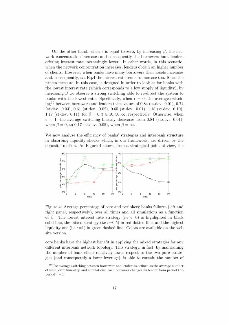
On the other hand, when ✏ is equal to zero, by increasing �, the net-work concentration increases and consequently the borrowers hunt lenderso↵ering interest rate increasingly lower. In other words, in this scenario,when the network concentration increases, lenders obtain an higher numberof clients. However, when banks have many borrowers their assets increasesand, consequently, via Eq.4 the interest rate tends to increase too. Since thefitness measure, in this case, is designed in order to look at for banks withthe lowest interest rate (which corresponds to a low supply of liquidity), byincreasing � we observe a strong switching able to re-direct the system tobanks with the lowest rate. Specifically, when ✏ = 0, the average switch-ing10 between borrowers and lenders takes values of 0.84 (st.dev. 0.01), 0.74(st.dev. 0.03), 0.61 (st.dev. 0.02), 0.65 (st.dev. 0.01), 1.18 (st.dev. 0.10),1.17 (st.dev. 0.11), for � = 0, 3, 5, 10, 50,1, respectively. Otherwise, when✏ = 1, the average switching linearly decreases from 0.84 (st.dev. 0.01),when � = 0, to 0.17 (st.dev. 0.05), when � = 1.

We now analyze the e�ciency of banks’ strategies and interbank structurein absorbing liquidity shocks which, in our framework, are driven by thedeposits’ motion. As Figure 4 shows, from a strategical point of view, the

0 3 5 10 50 inf

beta

3%

4%

5%

6%

7%

8%

ave

. p

erc

en

tag

e o

f co

re f

ailu

res

0 3 5 10 50 inf

beta

0%

1%

2%

3%

4%

ave

. p

erc

en

tag

e o

f p

erip

he

ry f

ailu

res

Figure 4: Average percentage of core and periphery banks failures (left andright panel, respectively), over all times and all simulations as a functionof �. The lowest interest rate strategy (i.e ✏=0) is highlighted in blacksolid line, the mixed strategy (i.e ✏=0.5) in red dotted line, and the highestliquidity one (i.e ✏=1) in green dashed line. Colors are available on the website version.

core banks have the highest benefit in applying the mixed strategies for anydi↵erent interbank network topology. This strategy, in fact, by maintainingthe number of bank client relatively lower respect to the two pure strate-gies (and consequently a lower leverage), is able to contain the number of

10The average switching between borrowers and lenders is defined as the average number

of time, over time-step and simulations, each borrower changes its lender from period t toperiod t+ 1.

17

banks’ failures. However, as shown for the number of incoming links and theleverage (see Fig. 2-3) when the intensity of choice becomes very high (i.e� > 10), the mixed strategy reaches the phase transition and, consequently,we observe a sharp increase in bankruptcies. This result clearly appears alsoin the analysis of the bad-debt of banks adopting the mixed strategy. Byobserving the middle column of table 2, in fact, we can notice the abruptjump in the banks’ bad-debt for � > 10. The e�ciency of the two purestrategies is, instead, strongly related with the interest rate and the lever-age motion. On the one hand, when ✏ is equal to one, by increasing theintensity of choice (and so the network centralization) the higher numberof core clients generates a too high core financial fragility and interest rate.Higher leverage coupled with higher interest rate increases the core fragilityvia two e↵ects. First, too much clients are detrimental for the core becausean increasing in the granted loan in not counterbalanced by an increasing inthe net-worth. Second, the too high interest rate paid by borrowers tendsto dramatically increase the core bad debt, as shown in the right hand sideof table 2.On the other hand, when ✏ is equal to zero, core banks, by increasing �, tendto o↵er too low interest rates. In this circumstance, the increasing numberof the core clients in not enough to compensate the very low profits givenby too low interest rates.When we analyze the e↵ect of the three strategies on the periphery banksby varying the intensity of choice (see right panel of fig. 4), we observe avery di↵erent behavior. It is important to notice that, in this circumstancestrategies are reversed. Specifically, when ✏ is equal to one the peripherybanks apply a strategy which o↵ers low rates in the face of a small liquiditysupply, on the other hand, when ✏ equals zero, they apply higher rates inreturn for a high liquidity. This is simply due to the fact that the peripheryhas a fitness measure opposite to the core. By analyzing this populationwe learn an important lesson. In this scenario, the lenders requiring higherinterest rates (i.e ✏ = 0) are more resistant to face shocks. By increasing�, all three strategies face a contraction in the number of customers, whichis particularly evident at � greater than 5 (see bottom right panel in fig.2). The dynamic in the periphery in-degree is, however, quite similar for allthe three strategies, what changes, instead, is the behavior of the interestrate (see bottom right panel in fig. 3). Periphery banks using the strategy✏ = 0 are able to apply higher rates (with a maximum around 11%) but,otherwise, they never reach a level of the rate as high as to be detrimentalto them as, however, is the case of core banks under the strategy ✏ = 1. Themodel, then, identifies a minimum and a maximum interest rate, above orbelow which banks fail or for low profits or for insolvent customers.

18

4 Concluding remarks

In this paper we have studied, in a very simple framework, the impact ofdi↵erent network topologies on banks’ financial fragility. By implementingan endogenous attachment mechanism which evolves via a fitness measurebased on three di↵erent banks’ strategies, we have investigated how sys-temic risk emerges from the interaction and which network topology andbank strategy are more resilient against the random attack to vertices. Inall the investigated scenarios, our findings have shown that the system vul-nerability is strongly related with the network concentration. When in theinterbank system we have very few hubs acting as lenders, we observe highleverage often associated with high financial fragility. Network concentra-tion leads hubs (i.e lenders) to grant too much credit compared to theirequity and, consequently, in the unlike event of shock, to be overwhelmedby their debtors’ insolvency. We have shown that this result holds evenif hubs charge high interest rates in return for their high liquidity supply.The application of this strategy, in fact, produces strong negative feedbacks.On the one hand, hubs grant too much loan with respect to their liquidityand, thus, become very illiquid in case of shock. On the other hand, byapplying too high interest rates to their borrowers, hubs are likely to havemany insolvent customers and, consequently, through the bad debt whicherodes their equity, to fail themselves. When hubs, otherwise, apply verylow interest rates to their clients, they su↵er from an excessive erosion oftheir profits that turns out to be very harmful. The model identify, then, amixed strategy which, by combining not too high (or too low) interest rateswith a network concentration below the transaction phase, appears to bethe most e�cient in case of liquidity shocks.

Acknowledgements

The research leading to these results has received funding from the Euro-pean Union, Seventh Framework Programme FP7, under grant agreementMATHEMACS, n0 : 318723 and FinMaP n

0 : 612955. The authors aregrateful for funding this research from the Universitat Jaume I under theproject P11B2012� 27.

References

[1] Albert, R., Jeong, H., Barabasi, A. (2000). Attack and error toleranceof complex networks, Nature 406, 378-382.

[2] Allen F, Gale D (2000) Bubbles and Crises. Economic Journal 110 : 236-55.

19

[3] Arcand, J.L., Berkes, E., Panizza, U. (2011): Too Much Finance?, work-ing paper.

[4] Barabasi A.L, Albert, A. (1999). Emergence of scaling in random net-works. Science 286, 509-512.

[5] Bartelsman E, Scarpetta S, Schivardi F (2005) Comparative analysisof firm demographics and survival: evidence from micro-level sources inOECD countries. Ind Corp Chang 14(3): 365-39.

[6] Battiston S, Delli Gatti D, Gallegati M, Greenwald B, Stiglitz JE(2007) Credit chains and bankruptcy propagation in production networks.Journal of Economic Dynamics and Control 31 : 2061-2084.

[7] Battiston S, DelliGatti D, Gallegati M, Greenwald BC, Stiglitz JE(2012a) Liaisons dangereuses: Increasing connectivity, risk sharing, andsystemic risk. J. of Economic Dynamics and Control.

[8] Battiston S, DelliGatti D, Gallegati M, Greenwald BC, Stiglitz JE(2012b) Default cascades: When does risk diversification increase sta-bility? Journal of Financial Stability, 8 (3): 138-149.

[9] Berger, Allen N and Klapper, Leora F and Udell, Gregory F., 2001.The ability of banks to lend to informationally opaque small businesses.Journal of Banking & Finance, 25 (12),2127-2167.

[10] Bernanke B, Gertler M (1989). Agency costs, networth, and businessfluctuations. American Economic Review 79(1):14-31.

[11] Bernanke B, Gertler M (1990) Financial fragility and economic perfor-mance. Q J Economic 105(1):87-114

[12] Bernanke B, Gertler M and Gilchrist, S. (1999) The Financial Accel-erator in a Quantitative Business Cycle Framework, in J. B. Taylor, andM. Woodford, eds., Handbook of Macroeconomics , Amsterdam: NorthHolland.

[13] Black, S.E., Strahan, P.E. (2002): Entrepreneurship and Bank CreditAvailability. Journal of Finance, 57(6), pp. 2807-2833

[14] Boss, Michael and Elsinger, Helmut and Summer, Martin and Thurner,Stefan 2004. Network topology of the interbank market. Quantitative Fi-nance, 4 (6), 677-684.

[15] Caccioli F, Catanach TA, Farmer JD (2012). Heterogeneity, Correla-tions and Financial Contagion. Advance in complex system, Vol. 15, Issuesupp02.

20

[16] Catullo, E., Gallegati, M., Palestrini, A. (2015). Towards a credit net-work based early warning indicator for crises. Journal of Economic Dy-namics and Control, 50 (0), 78-97.

[17] Chinazzi M, Fagiolo G, Reyes J A, Schiavo S (2012) Post-MortemExamination of the International Financial Network Working paper :http://dx.doi.org/10.2139/ssrn.1995499.

[18] Clauset A, Shalizi CR, Newman MEJ (2009). Power-law distributionsin empirical data. SIAM Rev 51(4):661-703. arXiv:0706.1062v2.

[19] Cocco J, Gomes F, Martins N (2009). Lending relationships in the in-terbank market. Journal of Financial Intermediation, 181, 24-48.

[20] Dabla Norris, E., Kersting, E. and Verdier, G. (2012): Firm productiv-ity, innovation and financial development, Southern Economic Journal,forthcoming.

[21] Dell’ Ariccia, Giovanni and Marquez, Robert, 2004. Information andbank credit allocation. Journal of Financial Economics, 72 (1), 185-214.

[22] Domencich T, McFadden D (1975) Urban travel demand. A behavioralanalysis. North-Holland Amsterdam.

[23] Ford JR., L.R., Fulkerson, D.R. (1956). Maximal flow through a net-work, Canadian Journal of Mathematics 8, 399-404.

[24] Ford JR., L.R., Fulkerson, D.R. (1962). Flows in Networks. PrincetonUniversity Press, Princeton, NJ.

[25] Greenwald BCN, Stiglitz JE (1993) Financial market imperfections andbusiness cycles. Q J Economic 108(1): 77-114.

[26] Grilli, R.; Tedeschi, G., Gallegati M. (2014): Bank interlinkages andmacroeconomic stability. International Review of Economics & Finance,34, 72-88.

[27] Grilli, R.; Tedeschi, G., Gallegati M. (2014): Markets connectivity andfinancial contagion. Journal of Economic Interaction and Coordination.doi:10.1007/s11403-014-0129-1.

[28] Grilli, R.; Tedeschi, G., Gallegati M. (2015) Network approach fordetecting macroeconomic instability. Proceedings of the IEEE 05/2015 ;DOI:10.1109/SITIS.2014.96.

[29] Hale G (2011). Bank Relationships, Business Cycles, and FinancialCrises. Working Paper 17356. National Bureau of Economic Research.

21

[30] Herrera, A.M., Minetti, R. (2007): Informed finance and technologi-cal change: evidence from credit relationships. Journal of Financial Eco-nomics, 83, pp. 223-269.

[31] Iori G, Jafarey S, Padilla FG (2006) Systemic risk on the interbankmarket. Journal of Economic Behavior & Organization 61 : 525-542.

[32] Issing, O. (2009): Some Lessons from the Financial Market Crisis.International Finance, 12, 3, pp 431-444.

[33] Kaushik R, Battiston S (2012). Credit Default Swaps Drawup Net-works: Too Tied To Be Stable? Working paper, arXiv:1205.0976v1.

[34] Lee, S.H., (2013). Systemic liquidity shortages and interbank networkstructures. Journal of Financial Stability 9 (1) 1-12.

[35] Lenzu, S., Tedeschi, G., (2012). Systemic risk on di↵erent interbanknetwork topologies. Physica A 3914331-4341.

[36] Levine, R. (2005): Finance and Growth: Theory and Evidence. In:Aghion, P. Durlauf, S. (2005): Handbook of Economic Growth, Elsevier,pp. 865-934.

[37] Lorenz J, Battiston S (2008) Systemic risk in a network fragility modelanalyzed with probability density evolution of persistent random walks.Networks and Heterogeneous Media 3.

[38] Memmel, C., Sachs, A., Contagion in the interbank market and itsdeterminants. Journal of Financial Stability 9 (1) 46-54.

[39] Maudos, Joaquın and De Guevara, Juan Fernandez, 2004. Factors ex-plaining the interest margin in the banking sectors of the European Union.Journal of Banking & Finance, 28 (9), 2259-2281.

[40] Minoiu C, Reyes J A (2011). A network analysis of global banking:1978-2009. Working Paper 11/74. IMF.

[41] Rajan, R.G., Zingales, L. (1998): Financial dependence and growth,American Economic Review, 88(3), pp. 559-586.

[42] Robinson, J. (1952): The Generalization of the General Theory, TheRate of Interest and Other Essays, Macmillan.

[43] Schiavo S, Reyes J, Fagiolo G (2010). International trade and financialintegration: a weighted network analysis. Quantitative Finance. 104, 389-399.

22

[44] Schumpeter, J. (1911): A Theory of Economic Development, HarvardUniversity Press.

[45] Sornette D, Von der Becke S (2011). Complexity clouds financeriskmodels. Nature 471, 166.

[46] Tedeschi G, Mazloumian A, Gallegati M, Helbing D (2012) Bankruptcycascades in interbank markets. PLOS One, 7(12), e52749.

[47] Tedeschi G, Vitali, S. Gallegati M. (2014). The dynamic of innovationnetworks: a switching model on technological change. Journal of Evolu-tionary Economics, 24, 4, pp 817-834

[48] Thurner S, Hanel R, Pichler S (2003) Risk trading, network topologyand banking regulation. Quantitative Finance 3 : 306-319.

[49] Tonzar, L., (2015). Cross-border interbank networks, banking risk andcontagion. Journal of Financial Stability (18), 19-32.

[50] Trichet, J. C. (2010). Reflections on the nature of monetary policynon-standard measures and finance theory. Opening speech at the ECBCentral Banking Conference. Frankfurt, 18 November 2010.

[51] Tridico, P. (2012): Financial Crisis and Global Imbalances: Its LabourMarket Origins and Aftermath, Cambridge Journal of Economics, 36(1),pp. 17-42.

[52] Vandenbossche J, Demuynck T (2013) Network formation with hetero-geneous agents and absolutefriction. Comput Econ 42 :23-45.

[53] Wray, L.R. (2009): The rise and fall of money manager capitalism: aMinskian approach, Cambridge Journal of Economics, 33(4), pp. 807-828.

23