
Simone Spampinati
224
UNIVERSITY OF NOVA GORICA GRADUATE SCHOOL STUDIES OF SCHEMES TO OBTAIN COHERENT VUV AND X- RAY PULSES: SEEDED HARMONIC GENERATION, SELF- SEEDING AND SELF- AMPLIFIED SPONTANEOUS EMISSION DISSERTATION Simone Spampinati Mentor: prof. dr. Giovanni De Ninno Nova Gorica, 2014
Transcript of Simone Spampinati

UNIVERSITY OF NOVA GORICA GRADUATE SCHOOL
STUDIES OF SCHEMES TO OBTAIN COHERENT VUV AND X-RAY PULSES: SEEDED HARMONIC GENERATION, SELF-
SEEDING AND SELF- AMPLIFIED SPONTANEOUS EMISSION
DISSERTATION
Simone Spampinati
Mentor: prof. dr. Giovanni De Ninno
Nova Gorica, 2014


UNIVERZA V NOVI GORICI FAKULTETA ZA PODIPLOMSKI ŠTUDIJ
ŠTUDIJ NAČINOV ZA GENERACIJO KOHERENTNIH PULZOV V VUV IN RENTGENSKEM PODROČJU
DISERTACIJA
Simone Spampinati
Mentor: prof. dr. Giovanni De Ninno
Nova Gorica, 2014


This thesis is dedicated to my parents and my brother.

Acknowledgments First I would like to thank my advisor, prof. Giovanni De Ninno, for giving me the opportunity to candidate me for a phd. I would also thank him for his support in these years and for his guidance to the completion of this thesis. I would also thank prof. G. Bratina and prof S.Stanic to have admitted me to the graduated school of the University of Nova Gorica. I would also thank prof S. Stanic for helps in the correction of the thesis. I want thank to who supported me with working positions during my phd: Emanuel Karantzoulis, Alessandro Fabbris, Stephen Milton, Michele Svanderlik and prof. Tor Raubenheimer. I would also thank Tor for a lot of discussions, suggestions and corrections of the thesis. I want thank to Luca Giannessi to have introduce me to the physics of free electron laser, for a lot of lessons and for an invaluable example of enthusiasm. I enjoyed a lot of great helps from my colleagues Alberto Lutman, Enrico Allaria, Laura Badano, Davide Castronovo, Max Cornacchia, Paolo Craievich, Miltcho Danailov, Alexander Demidovich, Yuantao Ding, Bruno Diviacco, Eugenio Ferrari, William M. Fawley, Lars Froehlich, Zhirong Huang, Henry Loos, Heinz-Dita Nuhn, Giuseppe Penco, Daniel Ratner, Carlo Spezzani, Cristian Svetina, Mauro Trovo’, Marco Veronese, Jihao Yi and Marco Zangrando during discussions and commissioning times in Trieste and at SLAC. Special acknowledgments go to Simone Di Mitri and Juhao Wu for a lot of discussions and lessons on accelerator and FEL physics. I want thank prof Shaukat Khan and David Newton for a lot of helps and corrections of the thesis. I want thank to my friends: Alberto, Alessandro, Andrea, Annalisa, Annamaria, Bibi, Chris, Claudio, Cristina, Daniele, David, Dennis, Fabrizio, Federico, Giacomo, Giusy, Lia, Luca, Laura, Marco, Matteo, Max, Sara, Stefano, Paolo, Pietro, Rytis, Tomasz, Valentina, Vincenzo. Finally, I thank my parents my brother Luca and my aunt Angela for their support and encouragements.


Abstract The need for coherent and intense pulsed radiation is spread among many research disciplines, such as biology, nanotechnology, physics, chemistry and medicine. Synchrotron light only partially meets these requirements. A new kind of light source, Free-Electron Laser (FEL), has been developed in the last decades to provide radiation in VUV/X-ray spectral region with characteristics beyond the reach of conventional light sources. In fact, FELs such as LCLS, FLASH and SACLA work regularly in the self ampli_ed spontaneous emission regime (SASE) producing short (<100 fs) and very intense (up to tens of GW) VUV and X-ray radiation pulses, characterized by good transverse coherence but poor longitudinal coherence, relevant shot-to-shot central frequency and power _uctuations. In this work we present the experimental results obtained using three techniques, aimed at further improving the spectral and temporal quality of SASE FEL light. The most promising technique is high-gain harmonic generation (HGHG). We will present the commissioning of FERMI@ELETTRA FEL1 line. Our activity provided a signi_cant contribution to the extension of harmonic generation in the deep VUV and X-ray regime. This required a careful optimization of the electron beam used to drive the FEL process. Our work focused in particular on the implementation of the laser heater system devoted to suppress microbunching instability. The second technique that will be described is self-seeding, applied to the hard X-ray regime. We will present the results of the experiments done at LCLS (to which we have actively participated) and the simulations that we have performed in order to interpret the obtained results. Finally, we have demonstrated the possibility to reduce dramatically the spectral width of SASE mode, generating isolated radiation spikes. The test experiment, on this scheme, carried at SPARC will be described here. In conclusion, this work provides new experimental results supporting the idea of using FELs as light sources capable of generating fully coherent and powerful pulses in the VUV and X-ray spectral regime, and con_rming the importance of the electron beam quality to reach spectral purity and high _ux of these pulses. Keywords: FEL, longitudinal coherence, microbunching, laser heater, seeding, HGHG, self seeding, tapering.


Povzetek
Potrebe po koherentnih pulznih svetlobnih izvorov z visoko luminoznostjo so skupne raznim znanstvenim področjem, biologija, nanotehnologija, fizika, kemija in medicina. Sinhrotronska svetloba samo delno izpolnjuje te zahteve. Z namenom, da bi ustvarili sevanje v spektralnem območju VUV (10 nm - 200 nm) in X (0.01 nm - 10 nm) z lastnostmi, ki presegajo zmožnosti konvencionalnih svetlobnih virov, je bila v zadnjih desetletjih razvita nova vrsta svetlobnih izvorov, t.i. "laserji na proste elektrone" (free electron lasers" ali FEL). FEL naprave, kot so Linac Coherent Light Source (LCLS) v ZDA, Free-electron-LASer v Hamburgu (FLASH) v Nemčiji in SPring-8 Angstrom Compact free electron laser (SACLA) na Japonskem običajno delujejo v načinu t.i. samo-ojačevane spontane emisije (SASE) ter generirajo kratke (<100 fs) in zelo močne (do več deset GW) svetlobne pulze v spektralnem območju VUV in X žarkov. Ti pulzi imajo dobro transverzalno koherenco, slabo longitudinalno koherenco in precejšnje fluktuacije centralne frekvence in moči med pulzi.
V disertaciji predstavljamo rezultate uporabe treh različnih tehnik za izboljšanje spektralne in časovne kakovosti pulzov, ki nastajajo v FEL pri načinu SASE. Za najbolj obetavno tehniko se je izkazalo generiranje višjih harmonikov z visokim izkoristkom (high-gain harmonic generation oziroma HGHG). Predstavili bomo zagon prve faze (FEL1) projekta FERMI@ELETTRA, kjer smo tehniko HGHG tudi uporabili in s tem pomembno prispevali k povišanju generiranja harmonikov v globoko območje VUV in X žarkov. Izvedba HGHG je zahtevala natančno optimizacijo žarka elektronov, ki se uporablja za generacijo svetlobnih pulzov v FEL. Osredotočili smo se predvsem na zagon grelnega laserja za odstranitev nestabilnosti elektronskega žarka v obliki mikro gruč. Druga tehnika, ki smo jo uporabili, je t.i. "self-seeding", ki se običajno uporablja v področju X žarkov najvišjih energij. Predstavili bomo rezultate eksperimentalnega dela na FEL napravi LCLS in simulacij, ki so bile potrebne za njihovo interpretacijo. V zadnjem delu smo, na podlagi eksperimentalnega dela na FEL napravi SPARC, predstavili nov način, ki bo lahko omogočal bistveno zmanjšanje spektralne širino SASE svetlobnih pulzov in generiranje ostrih konic SASE svetlobe.

Disertacija zajema skupek novih rezultatov, ki omogočajo uporabo FEL kot svetlobnih virov za generacijo popolnoma koherentnih svetlobnih pulzov z visoko luminoznostjo v spektralnem območju VUV in X žarkov. Rezultati prav tako potrjujejo, da je kakovost elektronskega žarka v FEL bistvenega pomena za doseganje spektralne čistosti in visoke luminoznosti izsevanih svetlobnih pulzov.
Ključne besede: laser na proste elektrone, FEL, longitudinalna koherenca, mikro gruče, generiranje višjih harmonikov z visokim izkoristkom, HGHG, grelni laser, časovno okno.

i
Contents
1 Introduction . . . . . . . . . . . . . . . . . . . . . . . . . . . . . . . . . . . . . . . . . . . . . . . . . . . . .1
1.1 Introduction . . . . . . . . . . . . . . . . . . . . . . . . . . . . . . . . . . . . . . . . . . . . . . . . . . . . 1 1.2 FEL principle and schemes . . . . . . . . . . . . . . . . . . . . . . . . . . . . . . . . . . . . . . . . 6 1.3 Electron beam requirements . . . . . . . . . . . . . . . . . . . . . . . . . . . . . . . . . . . . . . 14 1.4 Improving SASE . . . . . . . . . . . . . . . . . . . . . . . . . . . . . . . . . . . . . . . . . . . . . . .16 1.5 State of the art . . . . . . . . . . . . . . . . . . . . . . . . . . . . . . . . . . . . . . . . . . . . . . . . . 17 1.6 Thesis plan . . . . . . . . . . . . . . . . . . . . . . . . . . . . . . . . . . . . . . . . . . . . . . . . . . . 18
2 Particle accelerator and FEL theory . . . . . . . . . . . . . . . . . . . . . . . . . . . . . . . .19 2.1 Electron beam dynamics. . . . . . . . . . . . . . . . . . . . . . . . . . . . . . . . . . . . . . . . . .19 2.2 Magnetic bunch length compression . . . . . . . . . . . . . . . . . . . . . . . . . . . . . . . .30 2.3 Microbunching in high brightness electron beam . . . . . . . . . . . . . . . . . . . . . . 35 2.4 Particle and radiation dynamics in the FEL process . . . . . . . . . . . . . . . . . . . . 46
3 FERMI@ELETTRA, LCLS, SPARC . . . . . . . . . . . . . . . . . . . . . . . . . . . . . . .59 3.1 FERMI@ELETTRA . . . . . . . . . . . . . . . . . . . . . . . . . . . . . . . . . . . . . . . . . . . .59 3.2 LCLS . . . . . . . . . . . . . . . . . . . . . . . . . . . . . . . . . . . . . . . . . . . . . . . . . . . . . . . . 71 3.3 SPARC . . . . . . . . . . . . . . . . . . . . . . . . . . . . . . . . . . . . . . . . . . . . . . . . . . . . . . .78 4 FERMI linac . . . . . . . . . . . . . . . . . . . . . . . . . . . . . . . . . . . . . . . . . . . . . . . . . . . .83
4.1 Electron beam requirements . . . . . . . . . . . . . . . . . . . . . . . . . . . . . . . . . . . . . . 84 4.2 Emittance studies . . . . . . . . . . . . . . . . . . . . . . . . . . . . . . . . . . . . . . . . . . . . . . . 87 4.3 Longitudinal phase space optimization . . . . . . . . . . . . . . . . . . . . . . . . . . . . . 90 4.4 Design and implementation of a laser heater for FERMI . . . . . . . . . . . . . . . . 95 4.5 Commissioning of the FERMI laser heater . . . . . . . . . . . . . . . . . . . . . . . . . .104 4.6 Microbunching suppression . . . . . . . . . . . . . . . . . . . . . . . . . . . . . . . . . . . . . 112
5 FERMI FEL1 commissioning . . . . . . . . . . . . . . . . . . . . . . . . . . . . . . . . . . . .123 5.1 High gain harmonic generation . . . . . . . . . . . . . . . . . . . . . . . . . . . . . . . . . . 124 5.2 Low compression scenario . . . . . . . . . . . . . . . . . . . . . . . . . . . . . . . . . . . . . . .126 5.3 Mild compression scenario . . . . . . . . . . . . . . . . . . . . . . . . . . . . . . . . . . . . . . 140 5.4 Laser Heater and FEL1 performance . . . . . . . . . . . . . . . . . . . . . . . . . . . . . . 142 5.5 Extremely high harmonics . . . . . . . . . . . . . . . . . . . . . . . . . . . . . . . . . . . . . . .145 6 Self-seeding . . . . . . . . . . . . . . . . . . . . . . . . . . . . . . . . . . . . . . . . . . . . . . . . . . . 151 6.1 Self-seeding . . . . . . . . . . . . . . . . . . . . . . . . . . . . . . . . . . . . . . . . . . . . . . . . . .152 6.2 LCLS experiment: results . . . . . . . . . . . . . . . . . . . . . . . . . . . . . . . . . . . . . . . 155 6.3 LCLS self-seeding experiment: simulations and results analysis . . . . . . . . .163

ii
7 SASE with tapered undulator and chirp . . . . . . . . . . . . . . . . . . . . . . . . . . . .179 7.1 Compensation of linear chirp by undulator tapering . . . . . . . . . . . . . . . . . . .180 7.2 SPARC results . . . . . . . . . . . . . . . . . . . .. . . . . . . . . . . . . . . . . . . . . . . . . . . .183
8 Conclusions . . . . . . . . . . . . . . . . . . . . . . . . . . . . . . . . . . . . . . . . . . . . . . . . . . .191
Appendix A . . . . . . . . . . . . . . . . . . . . . . . . . . . . . . . . . . . . . . . . . . . . . . . . . . . .195

Chapter 1
Introduction
1.1 Introduction
Synchrotron radiation established itself, in the last decades, as one of the most important
tools for scienti�c discoveries through the implementation of techniques like di�raction,
spectroscopy, scattering and microscopy [1]. The achievable wavelengths cover the range
from hard X-rays to infrared light. One of the most important �gures of merit of synchrotron
radiation facilities is the spectral brightness, which de�nes the photon �ux per unit area, unit
solid angle and unit spectral bandwidth. Typical synchrotron brightness values are around
1019 − 1021·(photons/s·mm2·mrad2·0.1%·bandwidth). Other important characteristics are
the bandwidth, the wavelength tunability and the pulse duration. Despite the obtained
successes, the light produced by synchrotron machines does not permit the realization of a
large class of experiments that require more intense and shorter light pulses, or a complete
coherence of the employed radiation. Light pulses delivered by synchrotron machines have
1
CHAPTER 1. INTRODUCTION 2
a time duration ranging between tens and hundreds of ps. Therefore, they are not suited to
resolve in time electronic and molecular dynamics, which evolve with time scales of the order
of tens or hundreds of femtoseconds [2, 3, 4]. Other classes of experiments on non-linear
phenomena require a single-shot photon �ux higher than that provided by synchrotrons [5,
6]. In order to meet these requirements, free-electron lasers (FELs) were proposed [7, 8, 9].
These devices can provide a peak brilliance many orders of magnitude higher than that of
synchrotron facilities. The brilliance of some synchrotron beamlines as well as of proposed
and existing FEL is shown in �gure 1.1 The improvement in terms of peak brightness of
the X-FEL projects with respect to a typical synchrotron source is evident.

CHAPTER 1. INTRODUCTION 3
Figure 1.1: Brightness of light sources based on synchrotrons and FELs. The improvementin terms of peak brightness of the X-FEL projects with respect to a typical synchrotronsource is evident. Courtesy of A. Nelson.
LCLS (linac coherent light source), FLASH (Free-Electron laser in Hamburg) and SACLA
(SPring-8 Angstrom Compact free-electron laser) [10, 11, 12] are three facilities just work-
ing in the soft X-ray regime (LCLS, FLASH, SACLA) and in the hard X-ray regime
(LCLS, SACLA) while a FEL working down to 20 nm has actually been commissioned
at FERMI@Elettra [13].
Temporal coherence [14] is the measure of the average correlation between the wave and

CHAPTER 1. INTRODUCTION 4
itself delayed by t, at any pair of times. The delay over which the phase and the amplitude
changes by a signi�cant amount (and hence the correlation decreases by signi�cant amount)
is de�ned as the coherence time τc. At t = 0 the degree of coherence is perfect whereas it
drops signi�cantly when the time delay increases to τ c. The coherence length Lc is de�ned
as the distance the wave travels in the coherence time. The coherence time is a measure of
the monochromaticity of the light, since by Fourier transformation:
τc '1
∆νLLc '
c
∆νL(1.1)
where 4νL is the spectral width of the wave (full width at half maximum, FWHM) and c is
the speed of light. The minimum possible duration (FWHM) for a wave with the spectral
bandwidth 4νL is:
4τL =0.44
4νL(1.2)
4νL4τL = c · 4τL4λL(λL)2
= 0.44 (1.3)
The equations 1.2 and 1.3 are valid for a pulse with Gaussian shape in time and frequency
while a pulse with a di�erent shape has a greater time-bandwidth product. It is clear,
from equations 1.1 and 1.3, that a pulse with a time-bandwidth product given by 1.3, i.e.
a Gaussian pulse, has the longest coherence length possible associated with a given pulse
duration. Any deviation of the time-bandwidth product value from 0.44 implies a reduc-

CHAPTER 1. INTRODUCTION 5
tion of the coherent length. The transverse coherence implies a de�nite phase relationship
between points separated by a distance L transverse to the direction of beam propagation.
The spatial coherence can be measured in a classic Young's slits interference experiment
[15]. The transverse coherence and the large photon �ux open up new perspectives for
single-shot imaging, allowing single pulse coherent di�raction imaging [16, 17].
Synchrotron radiation is temporally incoherent and characterized by only partial transverse
coherence. LCLS, FLASH and SACLA work regularly producing short and very intense
x-ray radiation pulse characterized by good transverse coherence but poor longitudinal co-
herence [18, 19], relevant shot to shot central frequency �uctuations and power �uctuations.
On the other hand, experiments in the vacuum ultraviolet (VUV) region producing com-
pletely coherent pulses have been performed at several test facilities such as DUV FEL
[20] at BNL laboratory, the FEL on the Elettra synchrotron ring in TRIESTE [21], SPARC
(Sorgente pulsate ampli�cata radiazione coerente) [22] in Frascati (INFN/ENEA/CNR) and
MAX 4 demonstrator in Lund [23]. The extension of the schemes applied and results ob-
tained by these facilities down to nm wavelength requires a careful design of the electron
beam source, as in the case of FERMI@Elettra [24]. Fully coherent pulses in the deep VUV
and X-ray regime will allow, for example, multi-dimensional spectroscopy [25, 26] of valence
excitations in molecules [27] and coherent electron-hole interaction [28], the probing of the
electron correlation in solids via inelastic X-ray scattering [29] with very high resolution
and TG [30, 31] formation in the sample with a nanometer scale spatial period.
The work presented in this manuscript reports some experiments devoted to improve lon-
gitudinal coherence and spectral purity and stability of VUV and X-FEL. We will analyse
results obtained at FERMI@Elettra, LCLS and SPARC. We will describe FEL schemes
CHAPTER 1. INTRODUCTION 6
and measurements related to these experiments. We will show that the FEL longitudinal
and transverse coherence, and the spectral quality, are in�uenced also by electron beam
properties. Then, we will discuss the way to optimize the electron beam in the context of
FERMI@Elettra.
1.2 FEL principle and schemes
Radiation production in a FEL [7] is based on the passage of a relativistic electron beam
through the periodic magnetic �eld of an undulator, generating emission at a resonant
frequency �xed by the electron energy and undulator period and magnetic �eld. Di�erent
types of undulator can be used. The most common are the planar and the helical undulators
[32]. The undulator axis coincides with the direction of propagation of the electrons and the
direction of propagation of the wave. The magnetic �eld is perpendicular to the undulator
axis. The plane undulator is formed by a series of alternating dipoles. The electrons follow
a sinusoidal trajectory in the plane containing the undulator axis and perpendicular to the
magnetic �eld of the undulator as shown in �gure 1.2.

CHAPTER 1. INTRODUCTION 7
Figure 1.2: Electron trajectory (green line) in a planar undulator. The magnetic �eld ofthe undulator forces the electron on a zig-zag path with a spatial period that copies that ofthe undulator.
In a helical undulator the electrons follow a helical path. The resonance wavelength that is
the central wavelength of the undulator on axis radiation is given by [32]:
λr =λU2γ2
(1 +K2
rms
)(1.4)
K =e0B0λUβmec
(1.5)
where K = Krms for a helical undulator and K =√
2 ·Krms for a planar undulator. Here
λU is the undulator period, γ is the Lorentz factor, e0 is the electron charge, B0 is the
on axis magnetic �eld generated by the undulator and me is the electron mass. K is the
undulator strength parameter. The transverse velocity of the electrons, which is driven
CHAPTER 1. INTRODUCTION 8
by the undulator magnetic �eld, couples through the Lorentz force to a co-propagating
electromagnetic wave at the same resonant frequency. The electric �eld of the wave must
be contained in the plane in which the electron moves [33]. The electrons interact with a
linearly polarized radiation in a planar undulator and with an elliptically polarized radiation
in a helical undulator. This interaction produces a spatial modulation at the scale of the
laser wavelength (bunching) into the electron beam. When the bunching is signi�cant,
the beam starts to radiate coherently, reaching intensities much higher than spontaneous
emission [34]. The co-propagating radiation can be provided by an external seed laser or
can be the spontaneous radiation produced by the beam in the undulator. In these two
cases we have respectively a seeded [8] and a self-ampli�ed spontaneous emission (SASE)
[35] FEL. Both seeded and SASE FELs can generate very short wavelengths, and in both
cases the ampli�cation of the radiation with the fundamental wavelength is accompanied by
the production of radiation at high harmonics of the fundamental with an energy decreasing
with the harmonic number [36]. An exponential instability in the �eld amplitude derives
from the self-consistently coupled equations that describe the FEL process [33]. The light
has a higher velocity with respect to that of the wiggling electrons and there is a slippage
of the radiation with respect to the electrons. When the resonance condition is satis�ed,
the light advances one wavelength for each undulator period. Electrons can communicate
with the ones ahead only if their separation is less than the total slippage NλR. N is
the total number of undulator periods. The SASE [35] scheme relies on the presence of a
(weak) bunching factor at any wavelength (shot noise), naturally present in the electron
beam at the entrance of the undulator [37]. The component of the shot noise matching
the undulator resonant wavelength is ampli�ed, leading to an exponential growth of the
CHAPTER 1. INTRODUCTION 9
spontaneous radiation [38]. The radiation power exponentially grows along the undulator
as P (z) ∝ P (0)e− zLG [39], where P (0) is the initial radiation power, LG is the so called
gain length, and z is the coordinate along the undulator, up to a saturation value given by
Psat ≈ ρPe where Pe = EI is the electron beam power and ρ is the Pierce parameter de�ned
as ρ = λU4πLG
[40]. SASE FELs require very high-gain as the input power given by noise is
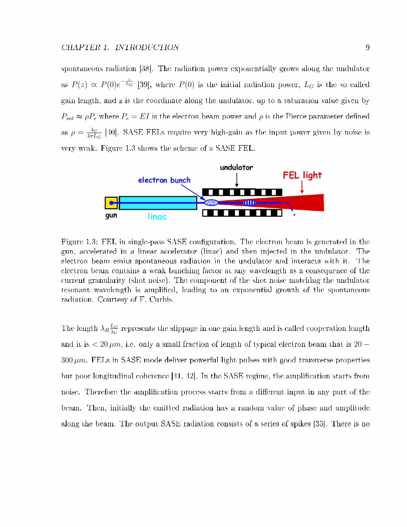
very weak. Figure 1.3 shows the scheme of a SASE FEL.
Figure 1.3: FEL in single-pass SASE con�guration. The electron beam is generated in thegun, accelerated in a linear accelerator (linac) and then injected in the undulator. Theelectron beam emits spontaneous radiation in the undulator and interacts with it. Theelectron beam contains a weak bunching factor at any wavelength as a consequence of thecurrent granularity (shot noise). The component of the shot noise matching the undulatorresonant wavelength is ampli�ed, leading to an exponential growth of the spontaneousradiation. Courtesy of F. Curbis.
The length λRLGλU
represents the slippage in one gain length and is called cooperation length
and it is < 20µm, i.e. only a small fraction of length of typical electron beam that is 20−
300µm. FELs in SASE mode deliver powerful light pulses with good transverse properties
but poor longitudinal coherence [41, 42]. In the SASE regime, the ampli�cation starts from
noise. Therefore the ampli�cation process starts from a di�erent input in any part of the
beam. Then, initially the emitted radiation has a random value of phase and amplitude
along the beam. The output SASE radiation consists of a series of spikes [35]. There is no
CHAPTER 1. INTRODUCTION 10
phase relation between the di�erent spikes and any spike identi�es a region over which phase
and amplitude correlation is established by the slippage of the radiation over the electrons.
The spikes' length is then equal to the cooperation length. Any SASE pulse contains tens
of longitudinal modes not correlated in phase and the bandwidth is therefore much larger
than the transform limited value of the pulse duration [35]. The stochastic nature of shot
noise causes a large shot-to-shot amplitude and wavelength �uctuation of SASE radiation
[35].
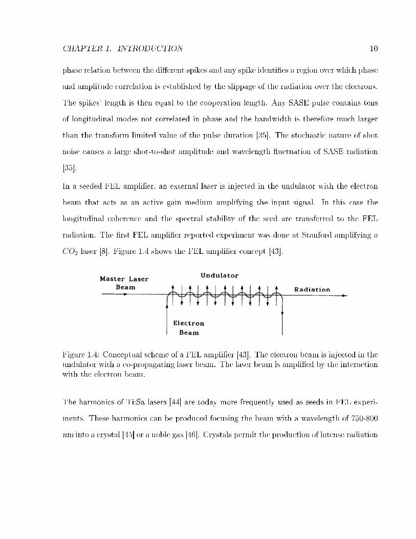
In a seeded FEL ampli�er, an external laser is injected in the undulator with the electron
beam that acts as an active gain medium amplifying the input signal. In this case the
longitudinal coherence and the spectral stability of the seed are transferred to the FEL
radiation. The �rst FEL ampli�er reported experiment was done at Stanford amplifying a
CO2 laser [8]. Figure 1.4 shows the FEL ampli�er concept [43].
Figure 1.4: Conceptual scheme of a FEL ampli�er [43]. The electron beam is injected in theundulator with a co-propagating laser beam. The laser beam is ampli�ed by the interactionwith the electron beam.
The harmonics of Ti:Sa lasers [44] are today more frequently used as seeds in FEL experi-
ments. These harmonics can be produced focusing the beam with a wavelength of 750-800
nm into a crystal [45] or a noble gas [46]. Crystals permit the production of intense radiation

CHAPTER 1. INTRODUCTION 11
beams at the second and third harmonic of the fundamental while the radiation emerging
from the gas contains higher harmonics [47]. As we have just seen, some harmonic con-
version and ampli�cation happens in the FEL too with an e�ciency decreasing with the
harmonic number. It is possible to increase the e�ciency at higher harmonics working with
two independent undulators, the second one being tuned to one of the harmonics of the �rst.
The external seed interacts with the electrons in the �rst undulator. The laser-electron in-
teraction produces energy modulation in the bunch at the wavelength of the laser. Then,
the beam goes through a magnetic device (dispersive section), in which the path length of
the electrons depends on their energy. In this way the energy modulation is converted in a
density modulation at the harmonics of the seed. The beam is now ready to emit coherently
in a second longer undulator (called radiator), tuned at one of the harmonics of the seed
laser. This scheme, called high-gain harmonic generation (HGHG) [48], is shown in �gure
1.5:
Figure 1.5: Scheme of a FEL working in the HGHG. The electron beam interacts withthe seed laser within the modulator. Here the beam energy is modulated by the laser.The energy modulation is converted in a density modulation, at the harmonics of the laserwavelength, in the dispersive section. FEL radiation is emitted in the radiator tuned at thedesired harmonic of the seed. Courtesy of F.Curbis.

CHAPTER 1. INTRODUCTION 12
Several seed FEL experiments in HGHG and in direct seeding con�guration have been
performed [20, 21, 22, 23]. HGHG can be repeated with a second stage composed of a
modulator, a dispersive section and a radiator following the �rst stage. In this case the
FEL radiation produced in the �rst radiator is used as a short wavelength high power seed
in the second modulator. A magnetic chicane can be placed between the �rst radiator and
the second modulator to delay the electron beam with respect to the seed. In this way the
FEL production in the second stage starts in a fresh part of the bunch. This method is
called the fresh bunch technique [49]. Figure 1.6 shows the fresh bunch scheme.
Figure 1.6: Fresh bunch scheme. The electron beam interacts with the seed laser in the �rstmodulator and it gains a spatial energy modulation at the laser wavelength. The energymodulation is converted in a density modulation, at the harmonics of the laser wavelength,in the �rst dispersive section. FEL light is produced in the �rst radiator that is tuned toa selected harmonic of the seed. This �rst HGHG stage is followed by another in whichthe light pulse produced in the �rst radiator is used to modulate the electron beam in thesecond modulator. The electron beam is delayed, by a magnetic chicane, with respect tothe FEL pulse before entering in the modulator. In this way the entire HGHG process, inthe second stage, happens in a fresh part of the bunch. Courtesy of L. Giannessi.
Up to now we have described high-gain single-pass con�gurations in which the radiation is
produced while the electrons make one single trip through the undulator line and is directly

CHAPTER 1. INTRODUCTION 13
extracted and used for experiments. FELs can work even in oscillator con�guration in
which the radiation is accumulated in an optical cavity during more trips of the electron
beam in the undulators [50]. This permits the use of a less bright electron beam and for
this reason it can be implemented even on storage rings, exploiting the high repetition
rate and stability of these accelerator machines [51]. On the other hand, the e�ciency of
optical cavities and mirrors is low in the extreme VUV and X-ray regime and therefore the
operations of oscillator FELs are actually limited to wavelengths longer than ≈ 200nm [52].
For this reason only single stage schemes have been studied and implemented in the VUV
and X-ray regime, even if also FEL oscillator schemes are proposed [53, 54]. This thesis
describes and discusses only single stage FELs. Figure 1.7 shows a FEL oscillator scheme
implemented on a storage ring FEL.
Figure 1.7: FEL oscillator on a storage ring. The radiation produced by the electrons inthe undulator is stored in an optical cavity and interacts with the electron beam in thefollowing turns. The undulator can be a single section or, as in the picture, a Klystroncomposed by two undulators and a dispersive section. Courtesy of F. Curbis.

CHAPTER 1. INTRODUCTION 14
1.3 Electron beam requirements
FELs operating in the VUV and X-ray regime, both in SASE and seeded con�guration
require a beam with high electron density in the six dimensional phase space. This requires
high current, low transverse emittance and low energy spread [55, 56]. The Pierce parameter
ρ, indicating the e�ciency of the interaction, has typical values in the X-ray regime of 10−4−
10−3 for a current of 500-3000 A. The high beam current is required to keep some e�ciency
and a relevant emitted power at very short wavelengths. The relative energy spread of
the electron beam at saturation is ≈ ρ. An initial relative energy spread approaching the
maximum value ≈ ρ, that occurs at saturation, greatly reduces the FEL interaction. Then,
it becomes clear that a low relative energy spread of the order of 10−4 of the electron
beam is of critical importance. The other beam parameter with a critical importance is the
normalized transverse beam emittance, εn = εγ, where the geometric transverse emittance
ε is a measure of the transverse phase space domain occupied by the beam [57]. A limit
on the geometric beam emittance for ensuring good spatial (transverse) coherence from
sources of spontaneous undulator radiation was derived in [58], giving εn <λ4π, where λ
4π
is the minimum phase space area for a di�raction limited photon beam. The ful�lment of
this requirement is necessary to obtain a matching of light and electron beam transverse
phase space, i.e. the radius and angular divergence of the electron and photon beams must
be matched to provide a good overlap and interaction between photons and electrons along
the undulator [59]. The above mentioned relation between geometric emittance and the
radiation wavelength gives a rough rule-of-thumb estimate of the electron energy/wavelength
possibilities. It shows, for example, that the minimum wavelength achievable decreases with
the normalized emittance, for a given beam energy and from this relation a requirement of

CHAPTER 1. INTRODUCTION 15
a normalized emittance in the range 1�3 mm·mrad comes out for a FEL in the VUV and
X-ray regime. Here all beam parameters are to be considered as slice parameters with a
slice length given by the FEL cooperation length.
The linear accelerators designed to drive the VUV and X-ray FELs have to deliver an
electron beam with very high quality. The design of most of the linacs proposed to drive
VUV and X-ray FELs includes a photoinjector [60] that represents the �rst part of the
machine to produce low emittance beam and one or more compressors to raise the beam
peak current. The electrons are produced by the impact of a UV laser on a copper cathode
placed in a �rst radio frequency (RF) cavity in which the electrons are accelerated to an
energy of few MeV (typically 4-6 MeV [61]). The �rst part of the photoinjector composed
of this �rst cavity is called the gun. Electrons emitted from the cathode are non-relativistic.
They repel each other transversally through Coulomb forces while space charge forces are
mainly longitudinal for relativistic electrons. Fast acceleration in the gun cavity is important
to obtain low emittance. The gun cavity is surrounded by a solenoid that compensates
Coulomb repulsion in the non-relativistic regime. Then the beam enters the following
booster sections placed at a distance from the gun imposed by the emittance compensation
scheme [62, 63, 64] and then the beam goes in a linear accelerator (linac) [65]. The bunch
is compressed in a magnetic bunch compressor. See [66] for a review of magnetic bunch
compression. Several phenomena, leading to a degradation of the beam quality can take
place in the linac and in the bunch compressors. Non-linearity in beam compressors [67]
and the microbunching instability [68] in the linac a�ect the beam longitudinal phase space
leading to a degradation of the beam FEL spectral purity [69]. We will introduce bunch
compression and microbunching instability in the next chapter. The accelerator scheme
CHAPTER 1. INTRODUCTION 16
described above is the one used in LCLS, FERMI, FLASH and other future FEL facilities
planed or in realization [70, 71].
1.4 Improving SASE
Several ideas have been proposed and partially tested to improve the spectral purity and
stability of SASE FELs. A �rst class of methods relies on the shaping of the longitudinal
electron-beam phase space, enabling the gain only in a small longitudinal portion of the
beam [72, 73], comparable to one cooperation length. In this case, the reduction of the
electrons involved in the photons production leads to a relatively low output power. An-
other method exploits a combination of a linear variation of beam energy along the beam
longitudinal coordinate (linear chirp) and a variation of the peak magnetic �eld (tapering)
along the undulator, to help the growth of a single spike. This scheme was proposed in [74]
and recently tested at SPARC [75]. Another technique to improve the spectral quality of
the SASE radiation is the so called self-seeding [76]. This technique has been recently tested
at LCLS [77]. The self-seeding scheme consists of a �rst SASE stage in which a pulse with
a peak power of GW level is produced in the soft or hard X-ray regime. Then, such a pulse
is used to produce a monochromatic seed for a second undulator line, tuned at the seed
wavelength. The seed coming from the �rst stage is eventually ampli�ed, up to saturation.

CHAPTER 1. INTRODUCTION 17
1.5 State of the art
The state of art in the �eld of X-ray regime and VUV light sources producing coherent
radiation is represented by SASE FELs [10,11,12] operating down to the hard X-ray regime
and by seeded facilities working in the VUV [13, 20-23]. SASE FEL's are capable of gener-
ating X-ray pulses ranging from hundreds down to tens of femtoseconds, allowing the direct
observation of structural dynamics [78, 79]. LCLS [10] is a single-pass SASE free-electron
laser driven by the SLAC linear accelerator. This light source has been in operation since
2009, generating pulses with a peak power of tens of GW. The shortest wavelength at LCLS
is 1.5·10−10m. LCLS is a SASE FEL. Therefore, the pulses are characterized by a stochas-
tic spiking structure in time and frequency. Every pulse contains tens of such spikes. As a
consequence, the coherence length is shorter than the pulse length and the pulse bandwidth
is longer than that determined by the pulse length. The short pulse duration (<100 fs)
and the high peak power per pulse (tens of GW ) permits to do time resolved experiments,
to study non-linear phenomena and to do di�raction of some single macro molecules like
viruses [80] and enzyme [81]. FLASH [11] in Hamburg and SACLA [12] in Japan are the
other facilities that use X-rays produced by FELs operating in SASE mode. FLASH reaches
1.5 nm and SACLA operates down to 0.7 · 10−10m. The operations of seeded FELs were
limited, before the commissioning of FERMI, down to 60 nm. These seeding experiments
are performed at SPARC [22], DUV-FEL [20] and at SPring-8 [82], and at the storage
ring Elettra's FEL [21]. Recently, the �rst commissioned FEL line of FERMI@Elettra [13],
named FEL1, generated powerful FEL pulses at 20 nm, the thirteenth harmonic of the seed
laser in one HGHG stage. Wavelength harmonic conversion down to the 29th harmonic [83]
in a single stage cascade has been demonstrated too. The commissioning of the second FEL

CHAPTER 1. INTRODUCTION 18
line of FERMI, FEL2, has started at the end of 2012 [84]. FEL2 works in two stage HGHG
scheme and uses the fresh bunch technique [59].
1.6 Thesis plan
This thesis reports some experiments devoted to improve longitudinal coherence and spectral
purity and stability of VUV and X-FEL. The structure of the thesis is the following. Chapter
2 is dedicated to presenting elements of beam and FEL physics. Chapter 3 introduces the
layout of the facilities in which the experiments described in this thesis are performed. In
Chapter 4 we describe the commissioning of the FERMI@Elettra linac. Chapter 5 describes
the results of FEL1 commissioning. Chapter 6 presents, self-seeding in the hard X-ray
regime, the results of self-seeding experiments performed at LCLS and related simulations.
Chapter 7 introduces a FEL scheme working with a chirped electron beam and a tapered
undulator and presents the experiment done at SPARC in this con�guration.

Chapter 2
Particle accelerator and FEL theory
In this chapter we introduce the basics of particle accelerator and FEL theory that will be
used in the following chapters.
2.1 Electron beam dynamics
Several techniques exist to accelerate charged particles [85]. Modern linear accelerators
(linacs) use radio frequency, RF cavities to accelerate particles to the �nal energy [65]. The
RF cavities provides a longitudinal electric �eld, whose typical frequency is from hundreds of
MHz up to few GHz. The motion of a charged particle in electromagnetic �elds is governed
by the Lorentz force:
F = e(E + v ×B) (2.1)
19

CHAPTER 2. PARTICLE ACCELERATOR AND FEL THEORY 20
where e is the particle charge, v is the particle velocity, E is the electric �eld and B is the
magnetic �eld. In this thesis we will treat only electrons for which e = e0 = 1.609 · 10−19C.
The energy gain/loss for an electron passing through a cavity is:
dE
dt= e0V0sin(ωrf t+ φ) (2.2)
where V 0 is the e�ective peak accelerating voltage and φ is the RF phase angle. In any
particle accelerator a reference trajectory, on which all particles should move, exists by
design. Electromagnetic guide �elds are used to force the particles to move on trajectories
close to the design orbit. The guide �elds are typically stationary magnetic �elds transverse
to the direction of motion. Dipole magnets are used to bend the particles trajectory on the
design orbit if this deviates from a straight path [86, 87]. These magnets de�ne the design
orbit for a reference particle with the nominal momentum p0. Particles in the bunch with
momentum p di�erent from the nominal one are bent di�erently and can go far away from
the designed orbit. A spread in the bunch of the initial position and momentum tends to
spread the particles transversely. Transverse focusing is thus used to limit the transverse
beam dimension. Focusing forces are usually provided by quadrupole magnets. Typically,
the design orbit lies within a plane and all magnets are oriented in such a way that the
particle motion can be decoupled in the horizontal and vertical direction. In the following
we assume that the trajectory lies in the horizontal plane only [87, 88]. It is convenient
to describe the motion of individual particles in terms of coordinates related to a reference
particle, with nominal momentum. At any longitudinal position s along the reference trajec-

CHAPTER 2. PARTICLE ACCELERATOR AND FEL THEORY 21
tory, the instantaneous position of a particle can be speci�ed by the curvilinear-orthogonal
coordinates (x, y, s). The horizontal and vertical displacements with respect to the design
orbit are then perpendicular to the tangent at the design orbit and are speci�ed by the
corresponding coordinates x and y in a local right-handed rectangular coordinate system
as shown in �gure 2.1a. The dipoles are rectangular magnets. Their longitudinal axes are
parallel to the longitudinal axis of the incoming beam. We consider dipoles with poles �at
and parallel to the horizontal plane. The magnetic �eld of these dipoles, By, is homogeneous
and directed along the vertical axis. The geometrical relationship between the trajectory
parameters inside the dipole are shown in �gure 2.1b.
Figure 2.1: a: Design orbit and coordinate system. Taken from [87]. b: Trajectory in adipole. Taken from [88].
The general equation of motion for an electron, choosing s as the independent coordinate
and retaining only terms up to the �rst order in the dependent variable, with a momentum
slightly deviating from the nominal is [86]:

CHAPTER 2. PARTICLE ACCELERATOR AND FEL THEORY 22
d2x
ds2= −Kx(s)x+
δ
ρ(s)= p0(1 + δ) (2.3)
where, terms of second and higher order in (x, y, d) are neglected. Here ρ (s) is the local
bending radius at the position s along the beam trajectory [86]. These equations describe
the focusing of electrons in the linear approximation. They are examples of Hill's di�erential
equation [89]. A proper arrangement of alternating quadrupole �elds is required to keep
particles close to the design trajectory simultaneously in both transverse planes [86]. The
function Kx(s) is piecewise assuming a speci�c value in any magnet sections. The solutions
of Hill's equation can be assembled from local solutions by means of transfer matrices. The
general solution of the homogeneous Hill's equation and its derivative can be expressed,
within an interval s0 ≤ s ≤ L, in terms of linearly independent solutions u1(s) and u2(s):
d2x
ds2= −Kx(s)x; x(s) = a1u1(s) + a2u2(s); x
′(s) = a1u
′
1(s) + a2u′
2(s) (2.4)
we can express the equations 2.4 in matrix form:
X(s) =
x(s)
x′(s)
; X(s) = U(s)A; U(s) =
u1(s) u2(s)
u′1(s) u
′2(s)
; A =
a1
a2
(2.5)
The matrix equation, yielding a representation of the general solution in terms of the initial

CHAPTER 2. PARTICLE ACCELERATOR AND FEL THEORY 23
conditions X(s0) at s0, can be expressed as:
X(s) = Mx(s, s0)X(s0); M(sn, s0) = M(snsn−1) · .....M(s1, s0) (2.6)
Where M is the transfer matrix. A similar formalism is applied to the y plane. The transfer
matrix can be written in the following way:
M(S, S0) =
C(S) S(S)
C′(S) S ′(S)
(2.7)
where C and S are the cosine like and sine like solution of Hill's equation satisfying the
relations:
C(s0) = 1; C ′(s0) = 0; S(s0) = 0; S ′(s0) = 1 (2.8)
In general the matrices Mx and My have a di�erent shape in any speci�c magnetic ele-
ment. The representation 2.6 of the general solution of the Hill's equation is very useful in
accelerator physics, since the function K(s) is typically piecewise constant to a very good
approximation. The equation of motion can thus be solved locally yielding transfer matrices
for the single intervals in which Kx(s) is constant, specifying a particular lattice compo-
nent such as a quadruple or a dipole and the general solution can be calculated by matrix
multiplication as indicated by the second identity in 2.6. A solution of the inhomogeneous
equation 2.4 can be found by using Green's functions, yielding a particular solution d · η(s)
with [57, 90]:

CHAPTER 2. PARTICLE ACCELERATOR AND FEL THEORY 24
η (s) = S(s)
s∫s0
C(t)
ρ(t)dt− C(s)
s∫s0
S(t)
ρ(t)dt (2.9)
Physically, d ·η(s) is the horizontal o�set of an electron with relative momentum deviation
d from the design orbit at s, provided the electron was moving on the design orbit in a
small interval around s0. The function η(s) is called the momentum dispersion function.
The general solution of the inhomogeneous equation can be expressed using again matrix
notation:
x(s)
x′(s)
δ
=
C(s) S(s) η(s)
C′(s) S
′(s) η
′(s)
0 0 1
x(s)
x′(s)
δ
(2.10)
The equation is referred to the x plane. It is possible to extend the matrix formulation to
the two planes and include even the longitudinal motion. To this end the particle can be
represented by a vector X(x) where x = [x, x′, y, y
′, z, δ] and z is the longitudinal position
within the bunch relative to the beam centroid (z=0). We write the matrix equation of
the particles in the bunch in the six dimension phase space making some simpli�cations.
Assuming that the beam trajectory lies in the horizontal plane allows us to decouple the
motion in the two transverse planes and so to simplify the equations by setting those term
to zero in the matrix R that couple the two planes and the terms that couple energy into
vertical plane. For a transfer line in which RF cavities are absent the equation can be

CHAPTER 2. PARTICLE ACCELERATOR AND FEL THEORY 25
further simpli�ed to assume the form:
X(s) =
R11 R12 0 0 0 R16
R21 R22 0 0 0 R26
0 0 R33 R34 0 0
0 0 R43 R44 0 0
R51 R52 R53 R54 1 R56
0 0 0 0 0 1
X(s0) X(s) =
x
x′
y
y′
z
δ
(2.11)
Any element Rij of matrix R for a particular lattice component indicates the in�uence of
the value assumed by the coordinate j at the start of the element, on the coordinate i at the
end of the element. For example particles with di�erent energy move on di�erent paths in
a layout element in which R56 6= 0. Their longitudinal separation, if the other coordinates
are the same for the two particle and at the �rst order in the energy separation, evolves in
this way:
4′z = 4z +R56 · 4E (2.12)
where ∆′z, ∆z, and ∆
′E are the particle longitudinal separation before the element, after the
element and the relative energy separation of the two particles respectively. The general
solution of the homogeneous Hill's equation can be expressed in the phase-amplitude form
[87]:

CHAPTER 2. PARTICLE ACCELERATOR AND FEL THEORY 26
x(s) =√axβx(s)cos(φx(s) + φx,0) (2.13)
where βx,y(s) and φx,y(s) are the betatron and the phase function, while ax,y(s) and φx,y,1
are real constants specifying the particular solution, and the betatron phase. The beta
function in a given accelerator completely describes the lateral focusing properties of the
guide �eld and the signi�cant characteristics of the particle trajectories. The maximum
displacement of a particle from the design orbit at position s in the x and y planes are√axβ(s) and
√ayβy(s). The phase-amplitude solution allows an instructive interpretation,
which can be seen by combining x(s) and x′(s) according to [87]:
γxx2 + 2αxx
′+ βxx
′2 = ax γyy2 + 2αyy
′+ βyy
′2 = ay (2.14)
Equation 2.14 de�nes an ellipse in the coordinates space (x, x′) centred at(x, x
′) = (0, 0) and
with area πax,y. The particle motion can thus be interpreted as a movement on an ellipse
in phase space, whose shape varies along the accelerator according to the corresponding
transfer matrices while its area remains constant. The interpretation of the particle motion
in terms of a transforming ellipse in phase space is particularly helpful for describing the
development of an electron distribution r(x, x') under the linear dynamics described above.
Since the dynamics of a single electron is determined by its phase space coordinates (x, x'),
every electron within a certain phase space area will stay within this area if the boundary
is transformed according to the equation of motion. Since an elliptical area with centre
(0, 0) remains elliptical as shown above, the transformation of a few ellipse parameters

CHAPTER 2. PARTICLE ACCELERATOR AND FEL THEORY 27
is suited to describe the envelope of an electron ensemble in coordinate space. Because
of its importance the parameter a is called the Courant-Snyder invariant. The relation of
Courant-Snyder parameters to the ellipse geometry is sketched in �gure 2.2 [86].
Figure 2.2: Beam in x-x' space and Courant-Snyder parameters. Taken from [87].
The evolution of the electron beam distribution can be described by means of the following
covariance matrix evolving from an initial point s0 to a �nal point s1 according to the matrix
formalism:
σx =
〈x2〉⟨xx′⟩⟨
xx′⟩ ⟨
x′2⟩ σx(s) = Mxσx(s0)MT
x (2.15)
where we have indicated with 〈x〉and 〈x2〉 the �rst and second moment of the beam distri-
bution. The following relation can be demostrated [90]:

CHAPTER 2. PARTICLE ACCELERATOR AND FEL THEORY 28
εxβx(s) =⟨(x(s))2
⟩εyβy(s) =
⟨(y(s))2
⟩(2.16)
where the εx, called geometric emittance [90], is de�ned as:
εx =√det(σx) =
√〈x2〉 〈x′2〉 − 〈xx′〉2 (2.17)
is called the geometric emittance [90]. Emittance has the units of length and represents
the area ( root mea square, RMS) occupied by the beam in the x-x' space. The quantities⟨(x(s))2⟩, corresponding to the element(σx)1,1 of the covariance matrix, can be obtained
observing the bunch images at one screen and measuring the RMS size of the beam. Then
the product of beam emittance and the beta function at one point is determined. It is
possible to recover the Twiss parameters αx, βx and γx and the emittance at the point s0, if
it is the initial point of a quadrupole and if a screen for transverse measurements is placed
in the point s. The technique used to accomplish this is the quadrupole scan [90] and it
consists of measuring the beam size of the electron distribution on the screen as a function
of the quadrupole �eld strength for at least three di�erent quadrupole settings.
A simple application of bending magnets is represented by beam energy spectrometer lines
in which the beam energy distribution is characterized by analyzing the transverse pro�le
collected on a screen, in the bending plane. Particles with di�erent energy follow di�erent
trajectories in the spectrometer dipole. The horizontal dimension of the beam on the screen
is:

CHAPTER 2. PARTICLE ACCELERATOR AND FEL THEORY 29
σx =
√(σx)
2Twiss +
(ησγγ0
)2
; (σx)Twiss =
√βxεx,nγ
(2.18)
A measurement of σx, when all the other quantities entering in the equation are known
or estimated, yields a value for the slice energy spread. The mean energy γ is obtained
from the value of the magnetic �eld of the bending magnet that is needed to bring the
beam on the reference trajectory to the centre of the screen. The values of (σx)Twiss and η
can be calculated by the magnetic machine lattice and beam emittance. The value of the
dispersion η at screen location can be measured changing the beam energy and measuring
the change of the beam position on the screen. A �rst value of the energy spread can be
obtained neglecting the Twiss beam size and considering the measured beam size as the
pure chromatic one:
(σγ)Chromatic = γ0σxη
(2.19)
On the other hand even a beam with zero energy spread has a �nite beam size on the screen
due to beam emittance and to the size of the pixels composing its image. In analogy with
equation 2.20 we can de�ne these two contributions to the measured energy spread derived
from the Twiss parameters and pixel size:
(σγ)Twiss = γ0(σx)Twiss
η(σγ)pixel = γ0
∆pixel
η(2.20)
The energy spread terms (σγ)pixel and (σγ)Twiss indicate the screen resolution and the lattice
resolution. A better estimate of energy spread can be obtained subtracting in quadrature
(σγ)pixel and (σγ)Twiss from (σγ)Chromatic. Spectrometers have to be designed in order to

CHAPTER 2. PARTICLE ACCELERATOR AND FEL THEORY 30
maximize the dispersion and minimize the beam Twiss dimension on the screen. This
permits to maximize the pure chromatic dimension on the screen and to minimize (σγ)Pixel
and (σγ)Twiss .
2.2 Magnetic bunch length compression
Magnetic bunch length compression is carried out via ballistic contraction of the particles
path length in a magnetic chicane. The linac located upstream of the magnetic chicane is
run o�-crest to establish a correlation between the particle energy deviation with respect
to the reference particle and the z coordinate along the bunch. More precisely, the linac
phase is adjusted so that the bunch head has a lower energy than the tail. The leading
particles travel, in the magnetic chicane, on a longer path than the trailing particles due to
their lower energy. Since all particles of the ultra-relativistic beam travel in practice at the
speed of light, the bunch edges approach the centroid position and the total bunch length
is �nally reduced. Figure 2.3 shows the concept design of magnetic bunch compression. In
the following, we choose a longitudinal coordinate system such that the head of the bunch
is at z<0.
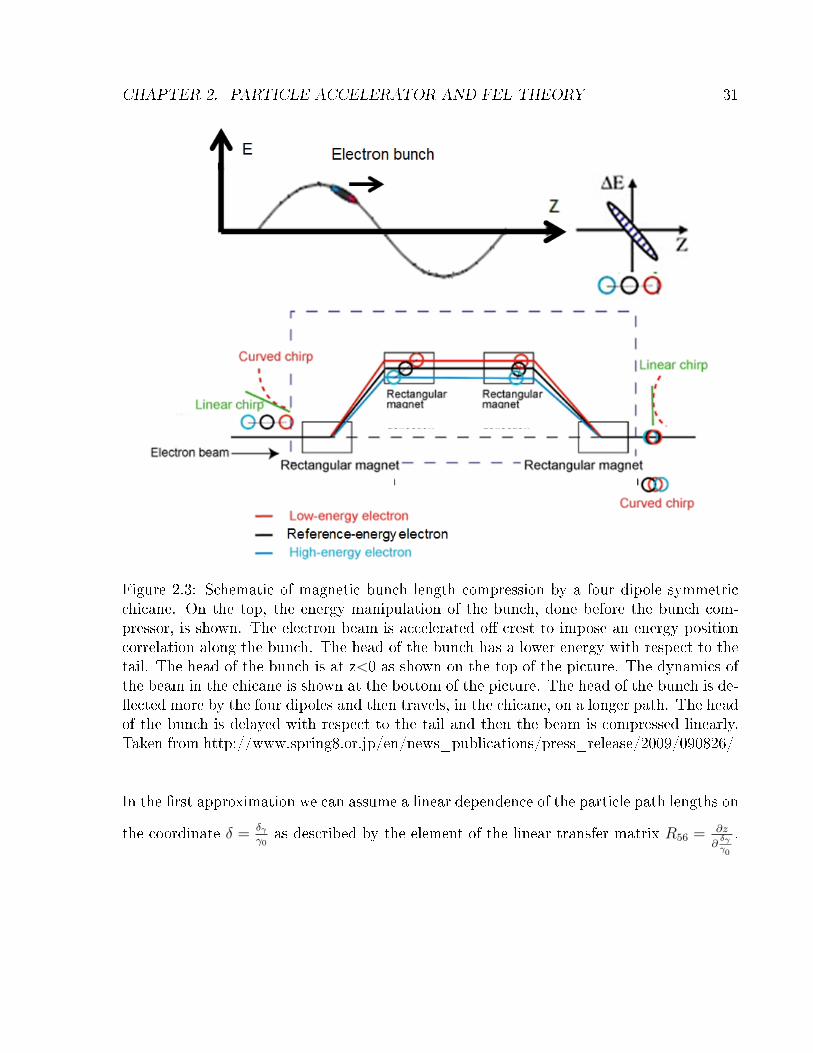
CHAPTER 2. PARTICLE ACCELERATOR AND FEL THEORY 31
Figure 2.3: Schematic of magnetic bunch length compression by a four dipole symmetricchicane. On the top, the energy manipulation of the bunch, done before the bunch com-pressor, is shown. The electron beam is accelerated o� crest to impose an energy positioncorrelation along the bunch. The head of the bunch has a lower energy with respect to thetail. The head of the bunch is at z<0 as shown on the top of the picture. The dynamics ofthe beam in the chicane is shown at the bottom of the picture. The head of the bunch is de-�ected more by the four dipoles and then travels, in the chicane, on a longer path. The headof the bunch is delayed with respect to the tail and then the beam is compressed linearly.Taken from http://www.spring8.or.jp/en/news_publications/press_release/2009/090826/
In the �rst approximation we can assume a linear dependence of the particle path lengths on
the coordinate δ = δγγ0
as described by the element of the linear transfer matrix R56 = ∂z
∂δγγ0
.

CHAPTER 2. PARTICLE ACCELERATOR AND FEL THEORY 32
The position occupied by a particle in the beam is modi�ed in the following way where zi
and zf are the particle's position in the bunch respectively before and after the chicane:
zf = zi +R56δγγ0
; R56 ≈ −2θ2
(d+
2
3leff
)(2.21)
where θ is the de�ection angle of any of the four magnet, d is the distance between the
�rst and the second magnet and between the third and the fourth magnet and leff is the
magnetic length of any of the fourth magnets. Also δγγ0
can be expanded up to the 1st order:
δγ
γ0
= hz (2.22)
A linac with energy gain E = eV · sin (φ) where V and φ are the peak accelerating voltage
and accelerating phase, imparts to the beam the following linear energy chirp:
h =d δγγ0
dz=
2π
λRF
e0V cos (φ)
E0 + e0V sin (φ)(2.23)
where E0 is the energy before the linac and λRF is the RF wavelength. The RMS bunch
length after compression is obtained, in the linear approximation, by substituting equations
2.22 and 2.23 into equation 2.21:
σz =⟨z2 − 〈z〉2
⟩≈ σz0 (1 + h ·R56) ; CF =
1
1 + h ·R56
(2.24)
where σz0 is the RMS bunch length before compression. The ratio between initial and �nal
bunch length, CF, is called compression factor. The peak beam current after compression

CHAPTER 2. PARTICLE ACCELERATOR AND FEL THEORY 33
is then I= CF · I0 where I0 is the initial beam current. The beam is compressed for CF> 1
and it implies h ·R56 < 0. R56 is negative, as seen by equation 2.24, and a positive chirp is
needed to compress the beam.
Up to now we are considering bunch compression in the linear approximation, assuming
that the compression process is linear in z and in ρ. In this approximation the di�erence
between the longitudinal position of a particle in the bunch before and after the chicane is
linear in z, zf − zi = R56hz, then any point of the beam is compressed by the same factor
asd(zf−zi)
dz= R56h. This means that, in the limits of validity of this approximation, the
bunch shape is preserved while the bunch length is compressed. In this limit it is possible
to obtain a �at current pro�le simply starting from a �at current distribution at the linac
entrance. A �at current is important, in a seeded and self-seeded scheme, to have a �at FEL
gain pro�le along the bunch preserving the Gaussian shape of the seed and then permitting
a FEL output pulse with a spectrum bandwidth close to the Fourier limit. In the real
case, second order terms are present in the path-length energy dependence of the chicane
transport matrix and in the electron energy-bunch position relation (second order chirp) as
the RF acceleration is governed by the sine function of the RF phase. The transformation
of the bunch longitudinal coordinate through the magnetic chicane and the quantity δγγ0
at
2nd order are:
zf = zi +R56δγγ0
+ T566
(δγγ0
)2
;T ≈ −3
2R56; (2.25)

CHAPTER 2. PARTICLE ACCELERATOR AND FEL THEORY 34
δγ
γ0
= hz + h′z2 h′ =d(δγγ0
)2
dz2
; h′=
1
2
dh
dz= −
(2π
λRF
)2e0V sinφ
E0 + e0V sinφ(2.26)
where T566 is the term of the chicane transport matrix with a second order dependence in
energy. It derives from equations in 2.25 and 2.26 that non-linear terms in energy-position
correlation and in the chicane transfer matrix are negligible for small compression factor,
CF<3. It can be found that the coupling between second order terms in the energy-position
bunch correlation and the chicane second order path-length dependence from the particle
energy leads to a non-linear compression for a linear compression factor greater than 3 [91].
In this regime, the di�erence between the longitudinal position of a particle in the bunch
before and after the chicane is no longer linear in z, as can be seen by equations in 2.25
and 2.26. Accordingly, the compression is not constant along the beam and this produces
a less homogeneous beam distribution, with formation of current spikes at the edges of the
electron bunch. An electron beam distribution as uniform as possible provides the maximum
peak current in the main body of the bunch and this improves the FEL gain and the photon
�ux. Limitation of the current spikes derived by non-linearity in the beam compression is
important, both for seeded and SASE scheme to avoid the strong longitudinal wake �elds
that can disrupt beam phase space as the beam travels along the high energy linac section
and the long undulator vacuum chamber usually characterized by a small gap and a high
impedance. The use of a short RF accelerating cavity, operated at a higher harmonic of
the linac RF frequency [92, 93], is usually adopted in order to linearize the 2nd order bunch
length transformation thereby maintaining the initial temporal bunch pro�le. In section 4

CHAPTER 2. PARTICLE ACCELERATOR AND FEL THEORY 35
experimental results of beam compression in FERMI bunch compressor are presented.
2.3 Microbunching in high brightness electron beam
The very bright electron beam required to drive VUV and X-ray FELs is susceptible to
a microbunching instability [68] that produces energy and current modulations [94-98] at
short wavelengths (≈ 1 − 5 µm). This collective instability takes place as linacs for FEL
light sources are equipped with bunch compressors designed to increase the peak current to
the level required for photon production. The microbunching instability was �rst foreseen
in [94] as a klystron-like mechanism of ampli�cation of density modulations, characterized
by some modulation periods, in an electron bunch compressed via a magnetic chicane. The
microbunching instability is presumed to start at the photoinjector exit growing from a
pure density and/or energy modulation caused by shot noise and/or unwanted modulations
in the photoinjector laser temporal pro�le. As the electron beam travels along the linac to
reach the �rst bunch compressor (BC1), the density modulation leads to an energy modula-
tion via (LSC). The resultant energy modulations are then transformed into higher density
modulations by the bunch compressor. This increased current modulation leads to further
energy modulations in the rest of the linac. Coherent synchrotron radiation in the bunch
compressor can also contribute to enhance the energy and density modulations and can even
increase the beam emittance [99, 100]. The modulations caused by the photocathode laser
temporal pro�le have usually a period of hundreds of microns [101] while shot noise spec-
trum has a white noise distribution and then some modulations are present even at shorter
wavelengths. Several studies [102-104] indicate that shot noise density modulations at the

CHAPTER 2. PARTICLE ACCELERATOR AND FEL THEORY 36
photocathode exit have amplitudes that can reach 0.01% while the modulations caused by
the laser modulation can reach ≈ 1. The presence, in the beam current distribution, of a
modulation with a speci�c period corresponds to a non-zero value of the bunching factor
at the corresponding wave vector: b(k) = 1Nec
∫I (z) e−kzdz [95]. The bunching factor as-
sociated with the shot noise can be estimated by the following formula b(k) =√
kecIb2π
[105].
The model for microbunching instability predicts that the beam, going into the bunch com-
pressor, gets energy modulations along the linac via the action of the longitudinal space
charge (LSC) coupled with the initial current density modulations. The LSC action can
be described by a longitudinal impedance model. The beam with a bunching factor b'(k)
gains an amplitude modulation given, in gamma units, by [95]:
∆m(k) = −I4πb′ (k)
Z0IA
∫ L
0
Z(k, s)ds (2.27)
The integral is from the beginning of the linac (≈ 100MeV ) to the bunch compressor loca-
tion and L is the length of this part of the linac in which energy modulations are accumulated
starting from the initial density modulations. Both shot noise and laser modulations have
characteristic scales shorter than the uncompressed bunch length. Thus they can be a driv-
ing term for space charge energy modulations. The expression of the longitudinal space
charge impedance is Z(k) = 4iZ0
kr2bl[1− krb
γK1
(krbγ
)]. The distribution function in the lon-
gitudinal phase space of the beam has the following form in front of the bunch compressor
[95]:

CHAPTER 2. PARTICLE ACCELERATOR AND FEL THEORY 37
f0(z′, δγ) = f0(z′, δ − hz′ − δm(z′)) (2.28)
where z is the longitudinal coordinate in the bunch, δ is the relative deviation ∆γγ0
from the
nominal beam energy γ0, h is the linear chirp used to compress the beam, δm(k) = ∆m(k)/γ0
is the relative amplitude of the energy modulation gained by the beam via LSC in the linac,
f0(z′, δ′ = ∆γ′/γ0) is the initial longitudinal distribution, z' and δ′are the longitudinal and
energy coordinates of a particle in the beam before compression. Equation 2.28 describes
the beam distribution function before the bunch compressor. The action of the compressor
is described by the change of variable z = z′ + R56[δ′ + hz′ + δm(z′)]. Thus, the energy
modulation is converted into an additional density modulation at a compressed wave number
kf = CF · k given by:
bf (kf ) =
∫dzdδf(z, δ)e−ikf =
∫dz′dδ′f0(z′, δ′)e
−ikf z′−ikfR56
[δ′+hz
′+δm(z′)
](2.29)
Now we use the linear approximation valid for small energy modulations such as |kR56δm| <<1
and we expand 2.29 as:
bf (kf ) = [b′(k)− ikfR56]
∫dδ′V (δ′)e−ikfR56δ′ (2.30)
When the initial density modulation can be neglected with respect to the chicane contri-
bution, as the �rst term in 2.30 can be neglected and the instability is said to be in the
�high-gain regime�. Now we express, in the high-gain regime, the gain in the density modu-

CHAPTER 2. PARTICLE ACCELERATOR AND FEL THEORY 38
lation after the �rst bunch compressor that is given by the ratio of the �nal over the initial
bunching [95]:
G (k) = |bfb′| ≈ I0
γIA|kfR56
∆γ(k)
γcompressor|∫dδ′V (δ′)e−ikfR56δ′ . (2.31)
The gain assumes the following expression when the initial energy distribution is Gaussian:
G (k) = |bfb′| ≈ I0
γIA|kfR56
∆m(k)
γcompressor|exp
(−1
2k2fR
256
σ2γ
γ2compressor
)(2.32)
Now we use the nominal parameters from the FERMI@Elettra conceptual design report
(CDR) [24] to calculate microbunching e�ects in one concrete example. The beam has a
charge of 800 pC, it is compressed by a factor 10 in a bunch compressor located at an
energy of 270 MeV with R56 = −41mm. Then the beam is accelerated to the �nal energy
of 1.2 GeV. The initial slice energy spread coming from the photoinjector, indicated as σ2γ
in the equation 2-32, is 3 keV. For this calculation we use only shot noise as a source of
the initial density modulation. The density modulation gain curve obtained by equation
2.32 is shown in �gure 2.4a. The blue curve is obtained for a Gaussian energy spread of
3 keV. The other curves in 2.4 are obtained for higher values of the initial energy spread.
The expression for the microbunching gain in the linear regime contains two terms. The
�rst one represents the conversion of energy modulation into density modulation for a zero
energy spread beam, while the exponential term in equation 2.32 represents the combined
action of slice energy spread and R56 in the bunch compressor. The �rst term is inversely
proportional to the modulation wavelength. The second term goes from zero to one for

CHAPTER 2. PARTICLE ACCELERATOR AND FEL THEORY 39
increasing modulation wavelengths. Modulations too short are smeared out by the combined
action of slice energy spread and R56 in the bunch compressor and then the gain is small at
short wavelengths. Longer modulation wavelengths are more resistant to the smearing in
the bunch compressor but the �rst term of equation reduces the gain as the spatial period
of the modulations becomes longer and longer. The gain curve presents a maximum and a
band of ampli�ed wavelengths as the two terms in equation 2.32 have opposite behaviours
with respect to the modulation wave vector. The bunching spectrum of the compressed
beam can be obtained from the gain curve and the initial bunching spectrum using the
high-gain approximation G (ki) ≈ | bind(kf )
bi(ki)|. The current modulations obtained by the beam
during bunch compression leads to further energy modulations in the rest of the linac via
longitudinal space charge. In �gure 2.4b we illustrate the spectrum of amplitude energy
modulations accumulated at the end of the linac calculated with the equations 2.27 and
2.32 starting from shot noise. The energy modulation spectrum shows a resonant behaviour
as the gain curve has a maximum and a band of ampli�ed wavelengths.
CHAPTER 2. PARTICLE ACCELERATOR AND FEL THEORY 40
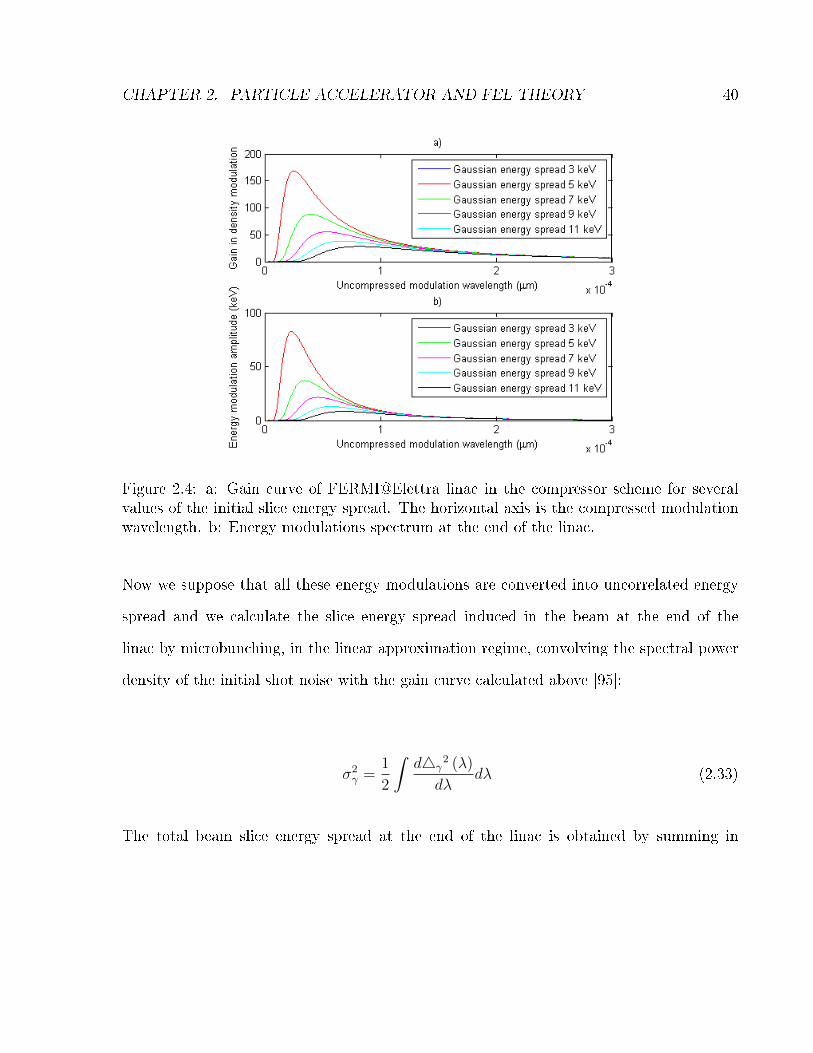
Figure 2.4: a: Gain curve of FERMI@Elettra linac in the compressor scheme for severalvalues of the initial slice energy spread. The horizontal axis is the compressed modulationwavelength. b: Energy modulations spectrum at the end of the linac.
Now we suppose that all these energy modulations are converted into uncorrelated energy
spread and we calculate the slice energy spread induced in the beam at the end of the
linac by microbunching, in the linear approximation regime, convolving the spectral power
density of the initial shot noise with the gain curve calculated above [95]:
σ2γ =
1
2
∫d4γ
2 (λ)
dλdλ (2.33)
The total beam slice energy spread at the end of the linac is obtained by summing in

CHAPTER 2. PARTICLE ACCELERATOR AND FEL THEORY 41
quadrature the energy spread given by the natural beam energy spread multiplied by the
compression factor that is applied to the bunch along the linac. We obtain a total slice
energy spread of 115 keV. The microbunching instability can take place because the beam
coming from the photoinjector is very cold [95, 102]. The exponential term in the ex-
pression for the density modulation gain shows that the particle longitudinal phase mixing
contributes to the suppression of the instability if the initial uncorrelated relative energy
spread σγγis su�ciently large with respect to the relative energy modulation amplitude ∆γ
γ.
In the case of non-reversible particle mixing in the longitudinal phase space (total suppres-
sion of the instability), this damping mechanism is called energy Landau damping. Figure
2.4a shows, as seen before, the gain curve, obtained from equation 2.32, for several values
of energy spread, considering a Gaussian energy distribution. It is evident that an uncorre-
lated energy spread higher that the natural one coming from the photoinjector e�ectively
reduces the microbunching gain. For this reason, a laser heater has been proposed to cure
and control microbunching instability in the linacs projected to drive VUV and X-ray FELs
[95, 106, 107]. This device can add a small controlled amount of energy spread to the elec-
tron beam in order to reduce the microbunching instability through Landau damping in the
bunch compressor [95, 106]. The laser heater consists of a short permanent magnet planar
undulator located in a small magnetic chicane through which an external laser pulse is su-
perimposed to the electron beam. The resulting interaction within the undulator produces
a modulation of the mean electron beam energy on the scale of the optical wavelength λL.
The mean beam energy, after the undulator has then the following variation with respect
to the beam longitude coordinate z:

CHAPTER 2. PARTICLE ACCELERATOR AND FEL THEORY 42
E(z) = E0 +4γLsin (kLz + φ0) (2.34)
where E0 and φ0 are the central beam energy and the phase between the laser and the
electron beam. The transverse dynamics in the last half of the chicane time-smears the
energy modulation leaving only an e�ective energy spread increase [95, 106]. The electron
distribution is modi�ed by the laser electron interaction in the undulator. Assuming initially
Gaussian distributions in energy and in the transverse coordinates, the electron distribution
function becomes [95]:
f0(z, δγ, r) =I0
ec√
2πσγexp{− [δγ −4γL(r)sin (kLz)]2
2σ2γ0
} 1
2πexp(− r2
2σ2x
) (2.35)
where kL = 2πλL, and σx = σy is the RMS electron beam size in the transverse plane and
r is the radial coordinate. The amplitude of the FEL energy modulation4γL(r) for a
fundamental Gaussian mode laser co-propagating with a round electron beam at the energy
in an undulator of length LU , which is short compared to both the Rayleigh length of the
laser and the beta functions βx,y of the electrons is [95]:
4γL(r) =
√PLP0
KLUσrγ0
JJ(K)exp(− r2
4σ2r
); JJ(K) = J0(K2
4 + 2K2)− J1
(K2
4 + 2K2
)(2.36)
where P0 = 8.7GW , PL is the laser power and K is the undulator parameter de�ned
by 1.5. Integrating the distribution function in 2.35 over the transverse and longitudinal
coordinates, we obtain the modi�ed energy distribution [95]:

CHAPTER 2. PARTICLE ACCELERATOR AND FEL THEORY 43
Parameter Vlaue
Electron beam energy 97 MevElectron beam size 130 µmLaser wavelength 783 nmLaser beam size 620 (130) µmLaser peak power 780 (32) µJ
Table 2.1: Laser heater parameters. Laser parameters in brackets are referred to the casein which the laser and the electron beam transverse sizes are matched.
V (δγ) =
∫rdr · exp(− r2
2σ2x
)
∫dξ√
4γL (r)2 − (δγ − ξ)2· exp
(− ξ2
2σ2γ0
)(2.37)
From the distribution 2.37 we obtain the RMS beam energy spread that is [108]:
σγ =
√(σγ0)
2 +σ2r
2 (σ2r + σ2
x)(4L(0))2 (2.38)
where 4L(0) is the on axis amplitude of the laser modulation. The total slice energy spread
is the sum of the initial energy spread and of the energy spread coming from the laser
heater action. We plot the energy distribution given by the equation 2.37 using laser heater
parameters from table 2.1, in �gure 2.5 for σr > σx (when the laser spot size is much larger
than the electron beam size, red curve ) and σr ≈ σx (when the laser spot size is matched
to the e-beam size, blue curve).

CHAPTER 2. PARTICLE ACCELERATOR AND FEL THEORY 44
Figure 2.5: Electron energy distribution after the laser heater for a larger laser spot (bluedashed curve) and for a matched laser spot (red solid curve). The laser powers are given intable 2.1.
When the spot size is much larger than the size of the electron beam the amplitude of the
energy modulation is almost the same for all electrons and the energy pro�le is a double horn
distribution. In this case Landau damping is not very e�ective because the two peaks in the
energy distribution are well separated and act like two di�erent electron beam populations,
reducing the mixing. On the other hand when the laser pro�le matches the transverse
dimension of the electron beam the energy modulation changes a lot across the transverse
pro�le of the electron beam. The resulting energy distribution is more uniform and the
mixing in the bunch compressor is more e�ective, reducing the microbunching gain. It is
possible to derive the expression for the gain of the bunching in the bunch compressor for
the beam heated by the laser heater [95] by inserting expression 2.36 and 2.37 in expression
2.31:

CHAPTER 2. PARTICLE ACCELERATOR AND FEL THEORY 45
G (k) = |bfb′| ≈ I0
γIA|kfR56
∆m(k)
γcompressor|SL (A,B) exp
(−1
2k2fR
256
σ2γ
γ2compressor
)(2.39)
SL (A,B) =
∫RdR · exp
(−R
2
2
)J0
[A · exp
(− R2
4B2
)];A = R56kf
4L
γ0
;B =σrσx
(2.40)
The energy spread σγ in equation 2.39 is the natural one coming from the photoinjector
and has a value of about 3 keV. We see that the maximum suppression is obtained when
the laser dimension matches that of the electron beam. For any value of the slice energy
spread added by the laser heater, taking B=1, we can calculate the �nal value of the slice
energy spread at the FERMI linac end. The result is plotted in �gure 2.5a. The �nal energy
spread is determined by the microbunching and by Liouville's theorem that states that the
area in the phase space is conserved. A compression by the factor CF of the bunch length
produces a growth of the initial energy spread proportional to the compression factor.
The Landau damping in the bunch compressor is not e�ective for a too small energy spread
and this produces an increase of the �nal slice energy spread. Increasing the initial energy
spread reduces the microbunching and the �nal slice energy spread. For a certain value of
initial energy spread the microbunchig instability is switched o� and then the �nal energy
spread, dominated by Liouville theorem, is proportional to the initial energy spread. The
curve in �gure 2.6a is only an approximation of the energy spread induced by micobunching
as we have used a linear model of longitudinal space charge ignoring the contribution of
the coherent synchrotron radiation (CSR) in the bunch compressor. The results obtained

CHAPTER 2. PARTICLE ACCELERATOR AND FEL THEORY 46
working with the linear model can be improved by a numerical multi-particle code and
numerical Vlasov solver. Figure 2.6b shows the energy spread at the linac end as a function
of the initial energy spread compressing the beam with one or two bunch compressors. The
two curves are referring to a bunch of 800 pC compressed by a factor 10 with one or two
compressors.
Figure 2.6: a: Final uncorrelated energy spread vs. initial slice energy spread. b: Final vs.initial uncorrelated energy spread for one and two stage compression in [email protected] solver simulation results taken from [97].
The results shown in �gure 2.6b, presented [97], are obtained with a Vlasov solver developed
by M.Venturini [96] and are in good agreement with the qualitative behaviour predicted by
the linear model.
2.4 Particle and radiation dynamics in the FEL process
The basic principle of the FEL emission relies on the interaction between a relativistic elec-
tron beam and a co-propagating electromagnetic wave in the presence of a static, periodic

CHAPTER 2. PARTICLE ACCELERATOR AND FEL THEORY 47
magnetic �eld. The magnetic �eld, provided by an undulator, induces electrons to move on
an oscillating trajectory. The transverse component of the electron velocity is then coupled
to the electromagnetic �eld propagating along the undulator axis. This interaction creates
a force along this direction and, depending on their phase with respect to the electroma-
gnetic �eld, electrons can gain or lose energy. As a consequence, the electron distribution
inside the bunch is modi�ed: the particles are distributed in micro-bunches separated by
the wavelength of the co-propagating radiation. The FEL process starts when there is a net
ampli�cation of the electromagnetic wave to the detriment of the electrons' energy. FEL
radiation occurs at the wavelength given by the resonance condition (1.4, 1.5). The FEL
process can be also seen as a stimulated emission/stimulated absorption process. The elec-
tromagnetic wave is ampli�ed (net gain) when the electron beam is slightly out of resonance,
because in case of perfect resonance half of the electrons gain energy and half lose energy.
FEL dynamics can be described by Maxwell and Lorentz equations in a 3D framework.
We consider a mono-energetic electron beam moving through an undulator generating a
magnetic �eld:−→BU = ∇×
−→AU . We assume the existence of a wave co-propagating with the
electron beam in the undulator:−→E = −1
c· ∂−→A∂t
and B = ∇×−→A . The total vector potential
is the sum of two components:
−−→Atot(z, t) =
−→AU(z) +
−→A (z, t) (2.41)
−→AU(z) =
aU√2
(−→e exp(−ikuz) + c.c) (2.42)

CHAPTER 2. PARTICLE ACCELERATOR AND FEL THEORY 48
−→A (z) = − i√
2(−→e ar(z, t)exp(−iΦr)exp(ikrz − iωzt) + c.c) (2.43)
where−→AU(z) is the undulator vector potential and
−→A (z, t) is the vector potential of the
wave. aU = BkU2
, kU = 2πλU
where λU is the undulator period and −→e = (−→x+i−→y )2
where are
the orthogonal unit vectors along the x and y axes transverse to the propagation axis z.
kr = 2πλr
= ωrc, Φr is the phase of the radiation �eld and ar = eλrE
2πmc2represents the amplitude
of the electromagnetic �eld, being E =∣∣∣−→E ∣∣∣ and e and m the electron charge and mass. Its
dependence on transverse coordinates (x and y) is neglected in the plane-wave and paraxial
approximation. Although the 3D model so far described is more general and accounts for
the three dimensional e�ects, here we want to review the simpli�ed model presented in
[40] which neglects transverse dimensions but captures the essential features of the FEL
process. We can derive the equations for electrons dynamics from the Lorentz equation.
Considering the electron phase θ = (kr + ku)z − ωrt relative to the radiation+undulator
�eld, which propagates in the z direction at the phase velocity vp = ωrkr+ku
, this expression
can be derived in order to get the evolution of the phase. Considering the de�nitions of the
vector potentials, and using the paraxial approximation ddt≈ cdt
dz, we can obtain the equa-
tions for the longitudinal evolution of electrons [109] in the one-dimensional (longitudinal)
approximation, the evolution of the electrons energy and phase are:
dγ
dz= −aUkr
γar(exp[iθ]− c.c.) (2.44)
dθ
dz= ku − kr
1 + a2U + iaU(arexp[iθ]− c.c.)
2γ2(2.45)

CHAPTER 2. PARTICLE ACCELERATOR AND FEL THEORY 49
The electromagnetic �eld obeys the wave equation where the source term is the average
over the electron beam cross section of the transverse current density [37, 39]. In the slowly
varying envelope approximation (SVEA), given by∣∣∂a∂z
∣∣ << |akr| and ∣∣∂a∂t ∣∣ << |aω|, thesecond order derivatives can be neglected and the equation for the �eld can be approximated.
Since −→a is slowly-varying on the scale of the radiation wavelength λ, the transverse current
can be average over a longitudinal distance of several wavelengths. Finally the equation for
the �eld evolution, neglecting the transverse variation of the electron and electromagnetic
�eld, in the 1D model can be written as:
(∂
∂z+
1
c
∂
∂t
)ar = kr
(ωpωr
)2
(arU
⟨exp(−iθ)
γ
⟩−⟨i
γar
⟩) (2.46)
where ωp =√
4πe2 nm
is the plasma frequency, with n the total electron number density.
The symbol 〈..〉 represents the average over a sample of N electrons of a given function:
〈f(θ, γ)〉 = 1n
∑Nj=1 f(θj, γj).
We de�ne now the energy-detuning parameter δr:
δr =1
ρ
〈γ〉2 − γ2r
γ2r
(2.47)
here 〈γ〉 is the mean electron energy at the undulator entrance and γr is the resonant energy.
In the regime we are interested in (i.e., the so called Compton regime), the energy of the
electron beam is high and the charge density is low, i.e., 1. The relative energy variation of
electrons is assumed to be:
∣∣∣∣γj − 〈γ〉〈γ〉
∣∣∣∣ << 1 (2.48)
CHAPTER 2. PARTICLE ACCELERATOR AND FEL THEORY 50
The derivative with respect to the time, in the equation for the �eld, can be neglected. The
coordinates z and t can be normalized with respect to the undulator length LU and to lb/c
(where lb is the bunch length) and therefore the ratio between the temporal and spatial
derivative coe�cients in the equation becomesLU(1−β‖)
β‖lb= NUλr
lbwhere NU is the number of
undulator periods. The term NUλrlb
represents the total slippage, i.e. distance between the
electrons and the radiation due to their di�erent velocities. When the total slippage is much
smaller than the bunch length lb, the time derivative can be neglected. This regime is called
the �steady-state regime" and its evolution depends only on the longitudinal coordinate.
The temporal coherence of the radiation is due to the slippage, because by means of this
mechanism the wave fronts can talk to each other. The radiation emitted by electrons in
the bunch tail interacts with electrons located as far as the total slippage length.
It has been shown that the �eld evolution, in the 1D model and steady state Compton
regime, along the longitudinal coordinate, from small to strong signal regime and using the
original variable z, can be reproduced by the following equations [110] where the so-called
fundamental FEL parameter or Pierce parameter is introduced:
PL(z) =P (0)
9
exp( zL1d
)
1 + P0
9Psat
[exp( z
L1d)− 1
] ; (2.49)
L1d =1
g=
λU
4πρ√
3; (2.50)
Lsat = L1dln(9PsatP (0)
); (2.51)

CHAPTER 2. PARTICLE ACCELERATOR AND FEL THEORY 51
Psat ≈ ρPe = ρIE; (2.52)
ρ = [
(I
IA
)·(λuAu2πσx
)2
·(
1
2γ0
)3
]13 ; AU = fc ·Krms (2.53)
where I is the electron beam peak current, IA = 17.05 kA is the Alfven current E is the
electron beam mean energy, σx = σy are the RMS transverse beam sizes, P (0) is the input
power and f c is 1 for an helical undulator and it is fc = K2rms
2·(1+K2rms)
for a planar undulator.
The gain function and the total gain can be written as:
G(z, δr) =|ar|2 (z)− |ar|20
|ar|20; (2.54)
G = gLU =LUL1d
= 4√
3πρNU ; (2.55)
The quantity L1d is the gain length in the 1D approximation. The saturation comes forz =
Lsat. The high-gain regime is characterized by G > 1. In our case ρ << 1, so that z
should be large enough, i.e., the undulator should be su�ciently long(LU >> L1d). In the
high-gain regime, the equation 2.49 is approximated, for z < Lsat, as:
PL(z) =P (0)
9exp(
z
L1d
) (2.56)
In the high-gain regime, the line width is [39]:
CHAPTER 2. PARTICLE ACCELERATOR AND FEL THEORY 52
4ωrωr≈ 4ρ (2.57)
An alternative picture of the resonance condition is given by the following statement: for
each undulator period where the electron passes through, the particle slippage with respect
to the wave should be equal to one wavelength of the radiation. This is equivalent to:
λU(c− v‖
)v‖
= λr (2.58)
Considering that 1γ2
= 1 − β2‖ − β2
⊥ = 1γ2− a3U
γ2and |β⊥| ≈ aU
γit is possible to derive the
resonance condition. When an electron beam starts to interact with an electromagnetic
wave, all the particles are randomly distributed in phase with respect to the wave, as shown
in �gure 2.7a.

CHAPTER 2. PARTICLE ACCELERATOR AND FEL THEORY 53
Figure 2.7: Bunching evolution. a: Electrons randomly distributed in phase (initial condi-tion: weak electromagnetic �eld). b: Electrons start bunching on a λs scale and the waveis ampli�ed. Courtesy of F. Curbis.
As the resonance condition is satis�ed, i.e. v‖ = vp = ωr(kr+kU )
half of the particles absorb en-
ergy from the electromagnetic wave and the other half transfer energy to the wave because
the particles tends to cluster where the ponderomotive phase is zero and hence the ampli-
�cation is zero. But, when the electromagnetic �eld of the ponderomotive wave changes a
lot, as in the high-gain regime, the phase velocity also changes, according to:
vp =ω − φkr + kU
(2.59)
As φ > 0, the latter relation states that the electrons act as a dielectric medium slowing
down the phase velocity of the ponderomotive wave. The velocity of the resonant electrons is
then v‖ > vp and they bunch around a phase where there is positive gain. Figure 2.8 explains

CHAPTER 2. PARTICLE ACCELERATOR AND FEL THEORY 54
the saturation mechanism, as it occurs in the electron phase space (θ, γ). The interaction
with the ponderomotive wave induces a modulation of the electrons energy. This energy
modulation evolves into a spatial modulation, also called bunching. When electrons exceed
the wave of a phase equal to a quarter of the ponderomotive force period there is maximum
gain. As the beam proceeds further inside the undulator, the spatial modulation arises also
where the ponderomotive force is positive and this causes �over-bunching�. Here the process
reaches the saturation because the electrons are not anymore able to transfer their energy
to the wave. The saturation is not a stationary state because the system does not arrive in
an equilibrium condition.

CHAPTER 2. PARTICLE ACCELERATOR AND FEL THEORY 55
Figure 2.8: Bunching evolution. a: Electrons randomly distributed in phase (initial condi-tion: weak electromagnetic �eld). b: Electrons start bunching on a λs scale and the waveis ampli�ed. Courtesy of F. Curbis.
So far the transverse dimensions of the electron beam and its angular divergence have been
neglected, as well as the di�raction of the light. Besides, the hypothesis of mono-energetic
beam (mentioned at the very beginning of the derivation of the equations) is far from
reality: an electron beam has an intrinsic energy-spread and this a�ects the performance of
the source. The emittance ε [90], de�ned by equation 2.14, is the quantity that takes into
account the transverse dimension and the angular dispersion of the electron bunch. The

CHAPTER 2. PARTICLE ACCELERATOR AND FEL THEORY 56
1D model gives the highest possible FEL gain (shortest gain length) and can be used as a
reference for the cases with non-ideal electron beam. In fact it can be shown from rigorous
analysis [111, 112] that the FEL gain length can be expressed by a universal scaling function:
L1d
LG= F (ηd, ηε, ηγ); ηd =
L1d
LR; ηε =
(L1d
β
)(4πε
λ
); ηγ = 4π
(L1d
λU
)(σ0
E0
)(2.60)
The universal scaling function can be determined by �tting the numerical solutions of the
coupled Maxwell-Vlasov equations describing FEL interaction and it is given by [55].
L1d
LG=
1
1 + η(2.61)
where:
η = a1ηa2d + a3η
a4ε + a5η
a6γ + a7η
a8ε η
a9γ + a10η
a11d ηa12γ + a13η
a14d ηa15γ + a16η
a17d ηa18ε ηa17γ (2.62)
and the 19 �tting parameters are given in [55]. The maximum of the scaling function
corresponds to the shortest gain length in the 1D limit L1d
LG= F (0, 0, 0) = 1. The scaling
parameters ηd, ηε and ηγ measure the deviation of the beam from the ideal case. Speci�cally,
ηd indicates the gain reduction due to the di�raction while ηε and ηγ measure the gain
reduction due to electron's longitudinal velocity spread caused by emittance and by energy
spread, respectively. Another scaling parameter related to the wavelength detuning has
been optimized to obtain the maximum gain thus eliminated to give the equations. The
saturation power obtained empirically by �tting simulation results and the evolution of the

CHAPTER 2. PARTICLE ACCELERATOR AND FEL THEORY 57
energy spread along the undulator are described by the following equations [113, 114]:
Psat = 1.6σ
(L1d
LG
)2
Pbeam; σγ(Z) =
√(σγ(0))2 +
9
4· ρ
Pbeam· (Psat − P (0)) · P (Z)
P (0)− P (Z) + 1.24(P (0)− P (Z))
(2.63)
where P (0), as sad in section 1.2, is the initial radiation power and σγ(0) is the initial
energy spread. In the case of SASE P (0) is provided by the shot noise and a shot noise
power Pnoise can be introduced. An approximation for shot noise power can be given by:
Pnoise(W ) = E (ρ)2 · c/λ (2.64)

CHAPTER 2. PARTICLE ACCELERATOR AND FEL THEORY 58

Chapter 3
FERMI@Elettra, LCLS, SPARC
In this chapter we describe the general layout of the three FEL facilities in which the
experiments described in this thesis were performed: FERMI@Elettra, SLAC and SPARC.
3.1 FERMI@Elettra
FERMI@Elettra [13, 24] is a single-pass FEL facility located at the Sincrotrone Trieste
Laboratory. The FERMI complex includes the following parts: a photoinjector generating
a bright electron beam [24, 115], the main linear accelerator in which the beam is time-
compressed and accelerated up to 1.2 GeV [24, 116], the system to transport the beam to
the undulators, the undulators generating the FEL radiation [24, 117], the photon beam
delivery system steering the radiation from the undulator to the experimental [118] area
and the experimental area itself [119-121]. The whole infrastructure is installed about 5 m
below ground level. Figure 3.1 shows a schematic plan (to scale) of the Elettra Laboratory.
59

CHAPTER 3. FERMI@ELETTRA, LCLS, SPARC 60
The circular building containing the Elettra synchrotron is visible at the centre. Below, the
FERMI@Elettra linac, undulator hall and experimental hall infrastructure is shown (the
electron beam goes from right to left).
Figure 3.1: Sincrotrone Elettra laboratory with the storage ring Elettra and the free-electronlaser FERMI. The circular building containing the Elettra synchrotron is visible at the cen-tre. Below, the FERMI@Elettra linac, undulator hall and experimental hall infrastructureis shown (the electron beam goes from right to left). Courtesy of G. De Ninno.
Figure 3.2 shows the layout of the FERMI accelerator.

CHAPTER 3. FERMI@ELETTRA, LCLS, SPARC 61
Figure 3.2: Layout of the Elettra beam accelerator of FERMI@Elettra: The electrons aregenerated in the gun by a copper cathode illuminated with a UV photoinjector laser andthen are pre-accelerated in the photoinjector that includes two booster cavities. The �rstlinac sections (L1) accelerate the beam and produce the chirp needed for bunch compressionin BC1. Linac1 includes a harmonic cavity used to linearize the compression. A secondbunch compressor, BC2, is placed after the other 5 cavities (L2 and L3). These cavitiesbring the beam to the �nal energy of 1.2 GeV (L4). The last two cavities, coloured in red,are two transverse de�ectors. The linac can be run with one or two compressors switchedon. Three spectrometer lines, used to measure the beam energy and energy spread after thephotoinjector and along the linac, are shown. The two cyan squares indicate two additionalcavities that can eventually be installed to increase the beam energy up to ≈1.5 GeV. Takenfrom [24].
The new low emittance RF photoinjector is based on the 1.6 cell electron gun [115] devel-
oped at BNL/SLAC/UCLA [122]. The beam is produced by the impact of a UV laser beam
(261 nm) on a copper cathode. The beam is accelerated in the gun cavity, composed of a
1.6 S-band cell up to an energy of ≈ 5MeV . The gun cavity is surrounded by a solenoid to
compensate for the transverse defocusing action of space charge that is very strong when
the beam is non-relativistic. Then the beam goes into two booster cavities, with the �rst
placed at a distance from the gun which is imposed by the emittance compensation scheme,
in which the beam is accelerated up to an energy of ≈ 100MeV . A compact diagnostic sec-
tion, equipped with a bending spectrometer, beam position monitors (BPMs), screens and
quadrupoles is inserted between the gun and the booster cavity. A transfer line equipped
with six quadrupoles, the laser heater system that is described in the section 4, beam posi-
tion monitors (BPMs), multi-screen diagnostic stations for beam pro�le measurement and

CHAPTER 3. FERMI@ELETTRA, LCLS, SPARC 62
a bending energy spectrometer is placed between the photoinjector and the linac [123]. The
measurement of the emittance and of the Twiss parameters are made, with the quadrupole
scan technique, using the last quadrupole before the laser heater chicane and the screen
placed after the laser heater undulator close to the electron beam waist location. Then
these data are used to determine the beam Twiss functions at the exit of the photoinjector
by backtracking. The quadrupoles of the transport line are used to transversely match the
electron beam to the linac. Figure 3.3 shows a 3D model of the low energy transfer line
that connects the photoinjector to the linac.
Figure 3.3: 3D model of the transfer line that connects the photoinjector with the linac.The �rst part of this transfer line includes four quadrupole magnets. This matching sectionis followed by the laser heater chicane, formed by four dipole magnets, that holds the laserheater undulator, screens for diagnostics and a BPM. A spectrometer is located in the lastpart of the transfer line. Courtesy of G. Penco.
The linac begins with a �rst stage called linac 1 (L1) composed by four CERN S-band
cavities working at 2.998 GHz, and an 1 X-band cavity used to linearize the electron beam
phase space before beam compression. The CERN cavities have an accelerating gradient

CHAPTER 3. FERMI@ELETTRA, LCLS, SPARC 63
of ≈ 15MV/m and the beam can reach an energy of 321 MeV when the RF phase, φ, is
set to 90 degrees. A 8.0 m long symmetric chicane, shown in �gure 2.4, is placed after L1.
It includes four identical bending magnets all powered by one power supply, two identical
quadrupole magnets in the lateral arms and four independently powered trim coils, each
of them associated with one bending magnet. These are intended for a �ne tuning of
the dispersion bump by compensating the �eld-to-current calibration errors in the dipole
�elds. Some electron beam diagnostics and machine protection device are located in between
the two inner bending magnets: one horizontal scraper, one BPM and one screen. The
design of the magnetic compressor derives from LCLS [124] and has been modi�ed with
some improvements of �eld homogeneity and movement accuracy and reproducibility. An
X-band cavity [125], working at the fourth harmonic of the S-band, is inserted in the
middle of L1 to linearize bunch length compression. The harmonic cavity is operated near
the deceleration crest lowering the beam energy by 20 MeV. Another transfer line [126]
is equipped with screens, BPMs, quadrupole, correctors, an energy spectrometer and a
vertical RF de�ecting cavity (low energy RF de�ector, LERFD) [127-129]. The beam can
be de�ected vertically by LERFD for beam slice measurements. The LERFD cavity is a
�ve cell standing wave structure, sharing the same klystron with the electron gun. After the
LERFD cavity, four quadrupoles and three multi-screens stations are placed for measuring
the beam optics parameters and matching them after the longitudinal compression. The
multi-screen stations are equipped with Optical Transition Radiation (OTR) [130] and
Yttrium Aluminium Garnet (YAG) targets [131]. This diagnostic station, located after
BC1, is shown in �gure 3.4.

CHAPTER 3. FERMI@ELETTRA, LCLS, SPARC 64
Figure 3.4: Diagnostic station after BC1. This transfer line is equipped with a transverseRF de�ecting cavity (LERFD) for beam slice measurements. After the LERFD cavity, fourquadrupoles and three multi-screens stations are placed for measuring the beam optics pa-rameters and matching them after the longitudinal compression. The multi-screen stationsare equipped with Optical Transition Radiation (OTR) and Yttrium Aluminium Garnet(YAG) targets. Courtesy of G. Penco.
The beam is then accelerated in three other CERN cavities and the seven Elettra cavities up
to an energy of 1.2 GeV. A second bunch compressor is placed in the linac before the last �ve
Elettra cavities (L4). The two bunch compressors allow continuously tunable compression of
the bunch length by a factor 1-50. The nominal compression factor of 10 [24] can be obtained
with a two stage compression or with BC1 only. The two schemes imply a di�erent balance
of the parameters characterizing the �nal electron beam quality, such as current and energy
�atness, emittance, slice energy spread, current and time jitter. Hence, they can be used
alternatively, according to speci�c FEL requirements. At the moment, the scheme with one
compressor is used to generate FEL light with high spectral purity for users experiments.
A 0.8 m long drift section, presented after each accelerating structure along the whole linac
provides focusing and trajectory control. It includes one quadrupole magnet with a bipolar
power supply, one BPM and two correctors. Another diagnostic area is present at the end of
the FERMI linac, including a horizontal high energy RF de�ecting cavity (HERFDX) [132],
a vertical high energy RF de�ecting cavity (HERFDY) [132] and the high energy (1.2-1.5

CHAPTER 3. FERMI@ELETTRA, LCLS, SPARC 65
GeV ) spectrometer beam-line, called Diagnostic Beam Dump (DBD). Figure 3.5 shows the
layout of the high energy diagnostic section.
Figure 3.5: Beam diagnostic area at the FERMI linac end. This transfers line includes ahorizontal RF de�ecting cavity (HERFDX) [132], a vertical RF de�ecting cavity (HERFDY)and the high energy (1.2-1.5 GeV ) spectrometer beam-line, called Diagnostic Beam dump(DBD). Courtesy of G. Penco.
The electron beam can be sent into one of the two FERMI undulator lines, FEL1 and FEL2,
through a system called spreader. The spreader starts with two 3 degree dipole bending
magnets that de�ect the beam away from the linac axis. Another pair of 3 degree bending
magnets de�ects the beam on the FEL2 line, which is parallel to the linac axis at a distance
of 1 m. The beam, when the �rst of the afore mentioned bending magnets are switched o�,
goes to another pair of bending magnets that brings it parallel to FEL2 line at a distance of
2 meters from it into the FEL1 line. Figure 3.6 shows a sketch (not to scale) of the FERMI
spreader.
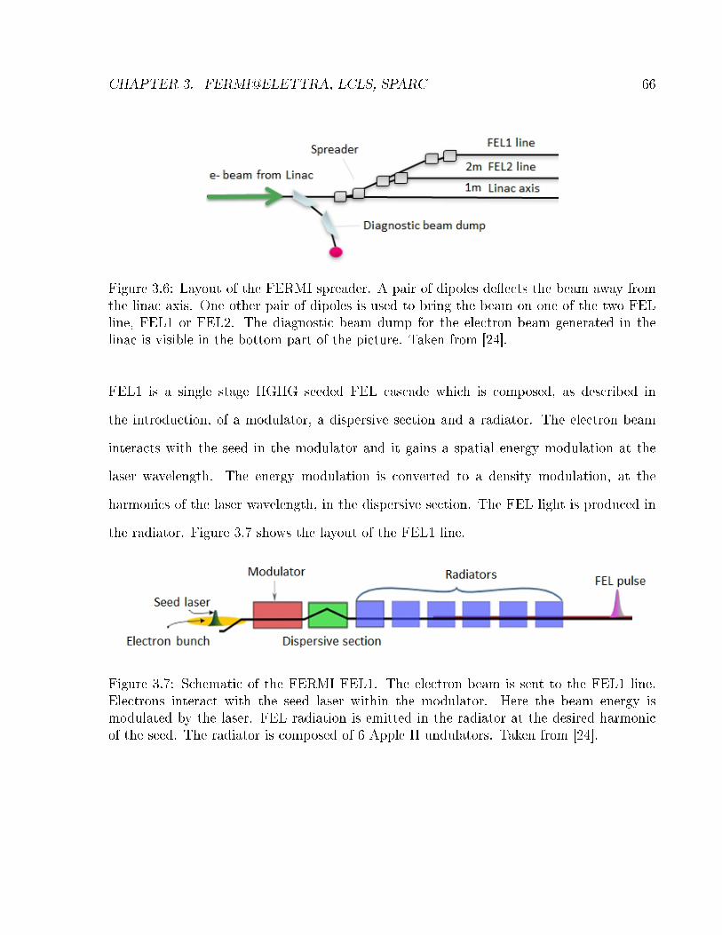
CHAPTER 3. FERMI@ELETTRA, LCLS, SPARC 66
Figure 3.6: Layout of the FERMI spreader. A pair of dipoles de�ects the beam away fromthe linac axis. One other pair of dipoles is used to bring the beam on one of the two FELline, FEL1 or FEL2. The diagnostic beam dump for the electron beam generated in thelinac is visible in the bottom part of the picture. Taken from [24].
FEL1 is a single stage HGHG seeded FEL cascade which is composed, as described in
the introduction, of a modulator, a dispersive section and a radiator. The electron beam
interacts with the seed in the modulator and it gains a spatial energy modulation at the
laser wavelength. The energy modulation is converted to a density modulation, at the
harmonics of the laser wavelength, in the dispersive section. The FEL light is produced in
the radiator. Figure 3.7 shows the layout of the FEL1 line.
Figure 3.7: Schematic of the FERMI FEL1. The electron beam is sent to the FEL1 line.Electrons interact with the seed laser within the modulator. Here the beam energy ismodulated by the laser. FEL radiation is emitted in the radiator at the desired harmonicof the seed. The radiator is composed of 6 Apple II undulators. Taken from [24].

CHAPTER 3. FERMI@ELETTRA, LCLS, SPARC 67
The modulator is a single planar undulator with variable gap that contains 30 periods of 10
cm. The dispersive section is an achromatic magnetic device with a non-zero R56 and zero
total dispersion. The R56 can be varied in the range 0− 130µm. The radiator is composed
of six Apple II undulators. Each 2.4 m long radiator section has a period of 55 mm. The
gap of the radiator can be changed from 10.5 mm to 220 mm to permit a wide tuning
of the FEL output. The minimum wavelength on which the radiator can be tuned with
K ≥ 1, considering an electron beam energy of 1.2 GeV, is 17 nm that corresponds to the
15th harmonic of the seed laser. The Apple II type helical undulator is a pure permanent
magnet structure composed of four arrays of magnetic blocks. There are four magnetic
blocks per period as shown in �gure 3.8.
Figure 3.8: Sketch of Apple II block con�guration. Each period contains 4 blocks, one foreach array. Taken from [24].

CHAPTER 3. FERMI@ELETTRA, LCLS, SPARC 68
The strengths of the vertical and horizontal magnetic �eld components can be varied, and
hence the polarization of the radiation produced, by moving two opposing magnet arrays
with respect to the other two along the undulator axis. The advantage of such a device
is that the radiation can be polarized vertically, horizontally, and circularly by moving
the arrays. Phase shifters [133] are installed in each section break between two radiator
sections, to maintain the right phase relation between the electron beam and the radiation
when passing from one undulator section to the next. A quadrupole for beam focusing and
a RF cavity BPM [134] are inserted in each undulator break. The seed can be the third
harmonic (266 nm) of a Ti:Sa infrared laser (780 nm) or the output of an optical parametric
ampli�er [135]. Two YAG screens placed at the two modulator ends permit the seed and
the electron beam to be transversely aligned. A fast photodiode, placed few meter before
the modulator, is used to measure the temporal delay between the seed and the transition
radiation produced by the electron beam passing through an OTR screen and provides a
clear time reference for the beams. Delays shorter than 6 ns are compensated with a delay
line for the seed laser while for greater delay it is mandatory to adjust the electronic trigger
in the seed laser. This coarse time synchronization, done with the photodiode, permits
the laser and the electron beam to overlap leaving a delay between the two of less than 10
ps. The �ne overlap can be obtained measuring the FEL pulse energy while moving the
delay line over a range of ≈ 50 ps. After leaving the undulators, while the FEL radiation
is transported to the experimental area, the electron beam is brought to a beam dump by
a sequence of bending magnets. Figure 3.9 shows the FERMI beam dump between the
undulator hall and the experimental hall.

CHAPTER 3. FERMI@ELETTRA, LCLS, SPARC 69
Figure 3.9: FERMI beam dump between the undulator hall and the experimental hall. TheFEL radiation is transported to the experimental area, while the electron beam is broughtto a beam dump by a sequence of bending magnets. Taken from [24].
The FEL system is completed by the photon diagnostics that are used to characterize the
FERMI FEL pulses and that are placed just before the beamlines. The FEL intensity can
be measured by means of two gas ionization cells [116, 136] placed between the undulator
hall and the experimental hall. Since only a very small portion of the FEL photons ionize
the gas, the method can be used online while the FEL is operating for users. The intensity
of single FEL pulses can be measured with a fast photodiode [136] that intercepts all of the
photons. The scheme of the layout used to measure the FEL energy is reproduced in �gure
3.10.
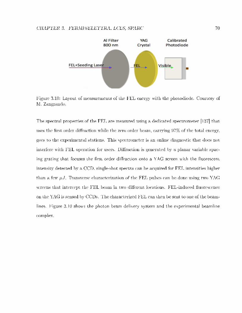
CHAPTER 3. FERMI@ELETTRA, LCLS, SPARC 70
Figure 3.10: Layout of measurements of the FEL energy with the photodiode. Courtesy ofM. Zangrando.
The spectral properties of the FEL are measured using a dedicated spectrometer [137] that
uses the �rst order di�raction while the zero order beam, carrying 97% of the total energy,
goes to the experimental stations. This spectrometer is an online diagnostic that does not
interfere with FEL operation for users. Di�raction is generated by a planar variable spac-
ing grating that focuses the �rst order di�raction onto a YAG screen with the �uorescent
intensity detected by a CCD. single-shot spectra can be acquired for FEL intensities higher
than a few µJ . Transverse characterization of the FEL pulses can be done using two YAG
screens that intercept the FEL beam in two di�erent locations. FEL-induced �uorescence
on the YAG is sensed by CCDs. The characterized FEL can then be sent to one of the beam-
lines. Figure 3.10 shows the photon beam delivery system and the experimental beamline
complex.

CHAPTER 3. FERMI@ELETTRA, LCLS, SPARC 71
Figure 3.11: Schematic of the FERMI experimental hall including the photon beam trans-port system and the three experimental chambers. The �rst part of the FEL front handincludes, for both FEL1 and FEL2, two ionization chamber intensity monitors and a gas cellproviding a wide range tunable intensity attenuation. Then, the light impinges on a variablespacing grating positioned to direct the �rst di�raction order, 3% of radiation power, ontoa YAG screen with �uorescent intensity detected by a CCD while the zeroth order goes toone of the experimental stations. This system permits to measure the FEL spectrum duringuser operation. Courtesy of D. Cocco.
FEL2 [84] is a double stage HGHG seeded cascade using the fresh bunch technique described
in section 1.2 and has a fundamental output in the range 4-20 nm. A su�ciently high �ux
at the third harmonic of the fundamental of the output radiator of FEL2 could reach that
part of spectrum at which the water is transparent, 2-4 nm and that for this reason is
particularly important for biological studies.
3.2 LCLS
The linac Coherent Light Source (LCLS) [61] is a SASE X-ray FEL facility in operation at
SLAC since mid-April 2009 [10]. Figure 3.8 shows the layout of the LCLS.
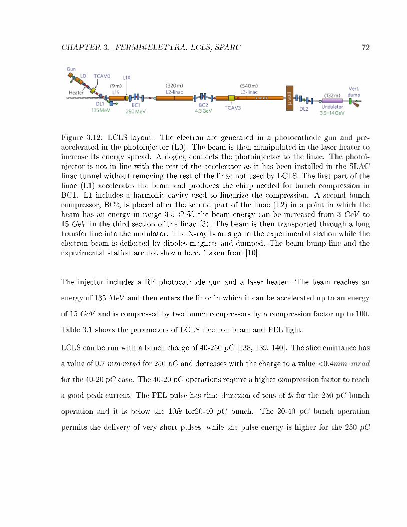
CHAPTER 3. FERMI@ELETTRA, LCLS, SPARC 72
Figure 3.12: LCLS layout. The electron are generated in a photocathode gun and pre-accelerated in the photoinjector (L0). The beam is then manipulated in the laser heater toincrease its energy spread. A dogleg connects the photoinjector to the linac. The photoi-njector is not in line with the rest of the accelerator as it has been installed in the SLAClinac tunnel without removing the rest of the linac not used by LCLS. The �rst part of thelinac (L1) accelerates the beam and produces the chirp needed for bunch compression inBC1. L1 includes a harmonic cavity used to linearize the compression. A second bunchcompressor, BC2, is placed after the second part of the linac (L2) in a point in which thebeam has an energy in range 3-5 GeV. the beam energy can be increased from 3 GeV to15 GeV in the third section of the linac (3). The beam is then transported through a longtransfer line into the undulator. The X-ray beams go to the experimental station while theelectron beam is de�ected by dipoles magnets and dumped. The beam bump line and theexperimental station are not shown here. Taken from [10].
The injector includes a RF photocathode gun and a laser heater. The beam reaches an
energy of 135 MeV and then enters the linac in which it can be accelerated up to an energy
of 15 GeV and is compressed by two bunch compressors by a compression factor up to 100.
Table 3.1 shows the parameters of LCLS electron beam and FEL light.
LCLS can be run with a bunch charge of 40-250 pC [138, 139, 140]. The slice emittance has
a value of 0.7 mm·mrad for 250 pC and decreases with the charge to a value <0.4mm ·mrad
for the 40-20 pC case. The 40-20 pC operations require a higher compression factor to reach
a good peak current. The FEL pulse has time duration of tens of fs for the 250 pC bunch
operation and it is below the 10fs for20-40 pC bunch. The 20-40 pC bunch operation
permits the delivery of very short pulses, while the pulse energy is higher for the 250 pC

CHAPTER 3. FERMI@ELETTRA, LCLS, SPARC 73
Parameter Value
Repetition Rate 1-120 HzBeam Energy 4.7-14.1 GeVBunch Charge 20-250 pCBunch length 15-400 fsPeak current 1.5-3 kA
Slice energy spread 1.5-4 MeVSlice emittance ≈0.4-1 mm·mradUndulator length 120 mUndulator period 3.0 cmUndulator K 3.5-3.46
Output wavelength 0.1-4 nm
Table 3.1: LCLS parameters.
bunch.
The LCLS undulator [141, 142] is 132 m long (including breaks for quadrupole magnets)
and was initially composed of thirty-three 3.4 m long planar, permanent magnet undulator
segments with 3 cm period, 6.8 mm full gap (�xed) height, and undulator parameter K=3.5.
The linac can be operated at any energy in the range of 3-15GeV. This permits the undulator
resonance and FEL output to be tuned in the range of 1− 40 · 10−10m wavelength. A break
occurs between each undulator magnet. A quadrupole magnet, an X-band cavity-type high
resolution beam position monitor (BPM) [143], a �beam-�nder wire� (BFW) and �exible
bellows are located at each break. Each undulator segment and its beamline components
are mounted on a remotely moveable support structure, called a girder [141]. The girder
motion is remotely controlled allowing the horizontal and vertical position to be changed, as
well as the yaw, the pitch and roll of the girders. Each girder hosts one undulator segment,
a quadrupole, a BPM, a beam �nder wire, a Cerenkov radiation detector for machine
protection and supports for the vacuum chamber. For obtaining and maintaining high-gain

CHAPTER 3. FERMI@ELETTRA, LCLS, SPARC 74
in the SASE process, it is important that the electron bunch has a good overlap with the
radiation �eld and that the individual electrons maintain a well de�ned phase relationship
with that �eld. The radiation �eld is initially produced in the �rst undulator segment and
proceeds in a straight line, while the electron beam trajectory deviates from a straight line
in the presence of magnetic and electric �elds. The electron beam trajectory straightness
requested by the FEL process depends critically on the wavelength and on the gain length.
The electron beam trajectory through the FEL undulator must be, in the case of LCLS
at the shorter wavelength of 1.5 · 10−10m, straight to a level of about 2 mm over one FEL
gain length (≈5 m) [144]. The ideal undulator magnetic �eld generates the tiny wiggling
motion, which is necessary for the FEL process; the �rst and second �eld integrals over
each undulator segment are ideally zero. Problems arise from o�-axis �elds of misaligned
quadrupoles and undulator segments, the earth's magnetic �eld [145], other environmental
�elds, as well as from errors in the undulator �elds that create �nite �eld integrals or increase
the electrons' path lengths through the undulator Alignment of all the undulator beamline,
the correction of the undulator �eld and the shielding and compensation of other magnetic
�eld is important to ensure the required straight electron trajectory All the components on
a girder are aligned on a coordinate measurement machine [146]. The girders are placed
in the tunnel and aligned by optical methods (laser tracker). Every undulator segment
is shielded against the magnetic �eld [145]. The remaining error-�elds (o�-axis �elds in
quadrupoles and undulator segments, the earth's magnetic �eld and the environmental
�eld) are corrected through beam based alignment [144], which compensates the net e�ect
of these �elds by adjusting the transverse positions of the quadrupoles, through girder
motion and by adding small dipole correction �elds through trim coil adjustments. This
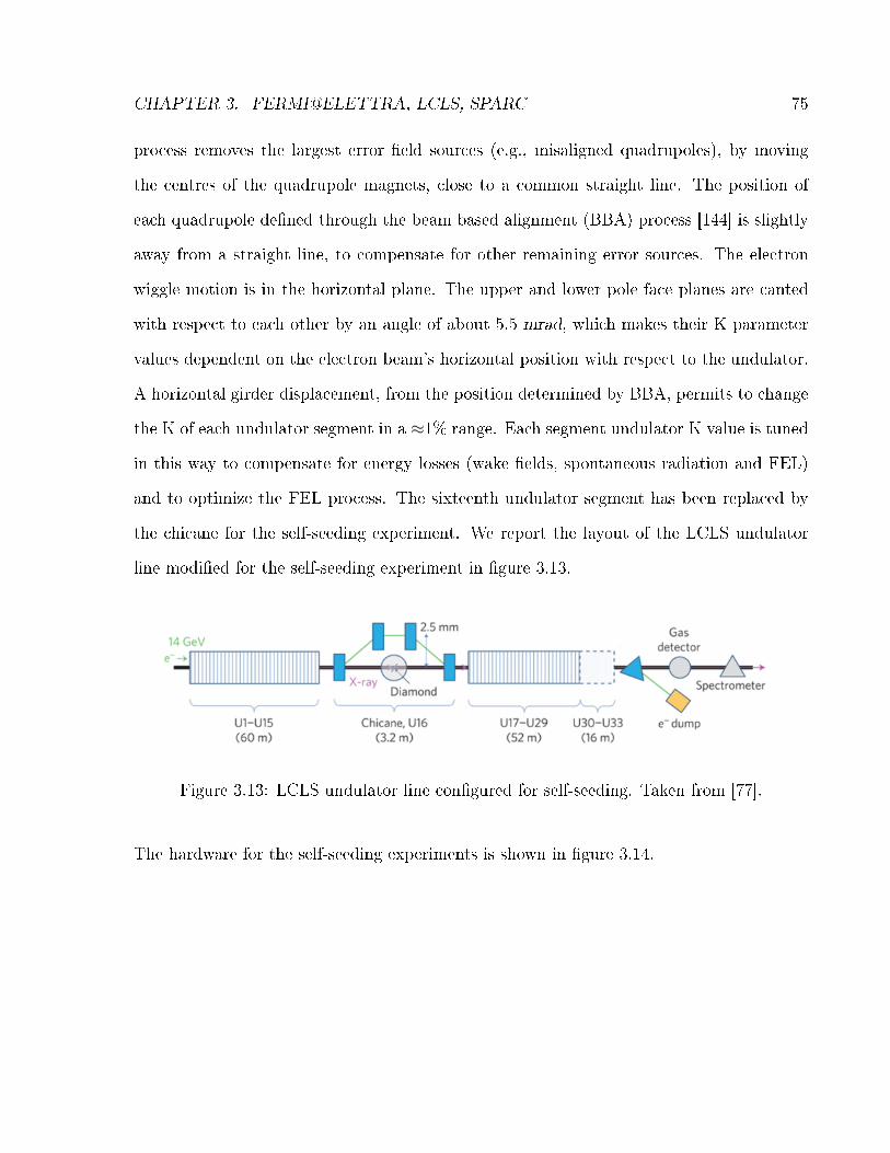
CHAPTER 3. FERMI@ELETTRA, LCLS, SPARC 75
process removes the largest error �eld sources (e.g., misaligned quadrupoles), by moving
the centres of the quadrupole magnets, close to a common straight line. The position of
each quadrupole de�ned through the beam based alignment (BBA) process [144] is slightly
away from a straight line, to compensate for other remaining error sources. The electron
wiggle motion is in the horizontal plane. The upper and lower pole face planes are canted
with respect to each other by an angle of about 5.5 mrad, which makes their K parameter
values dependent on the electron beam's horizontal position with respect to the undulator.
A horizontal girder displacement, from the position determined by BBA, permits to change
the K of each undulator segment in a ≈1% range. Each segment undulator K value is tuned
in this way to compensate for energy losses (wake �elds, spontaneous radiation and FEL)
and to optimize the FEL process. The sixteenth undulator segment has been replaced by
the chicane for the self-seeding experiment. We report the layout of the LCLS undulator
line modi�ed for the self-seeding experiment in �gure 3.13.
Figure 3.13: LCLS undulator line con�gured for self-seeding. Taken from [77].
The hardware for the self-seeding experiments is shown in �gure 3.14.

CHAPTER 3. FERMI@ELETTRA, LCLS, SPARC 76
Figure 3.14: Hardware for self-seeding installed on the girder of U16. The chicane forthe electron beam is formed by four magnets. The vessel containing the diamond and thediagnostics for the Bragg re�ection is installed in the middle of the chicane. Courtesy of P.Emma.
The 3.2 m long magnetic chicane installed at U16 includes four dipole magnets, which
displace the electrons horizontally by 2.5 mm to bypass the diamond monochromator. This
also nominally delays the electrons by 20 fs so as to overlap with the delayed monochromatic
X-ray seed pulse. Each chicane magnet is 36 cm long, separated from its neighbours by 58
cm and nominally bends the electron beam by 2.7 mrad with a magnetic �eld of 0.34 T, and
includes a 576-turn main coil and an independently powered 10-turn trim coil. This allows
the chicane to be adjusted between two di�erent con�gurations: (i) a self-seeded mode, with

CHAPTER 3. FERMI@ELETTRA, LCLS, SPARC 77
the electron delay set between zero and 40 fs using the main coils, and (ii) a much weaker
`phase-shift' mode, using the trim coils, with a delay of zero to10 · 10−10m (variable in
0.04 · 10−10m steps). The phase-shift mode (used during SASE operation) allows correction
of the electron-to-radiation phase error introduced by the removal of the 4 m long undulator
section at U16. This correction restores the full SASE X-ray pulse energy that was available
before the undulator section was removed. In addition, the dependence of the chicane path
length on electron energy, given by the R56 value of the transport matrix, washes out the
SASE-induced microbunching after the chicane, preparing the electron beam for coherent
seeding. With a typical relative electron energy spread of about σγ=0.01% RMS, the chicane
will wash out any temporal structure of wavelength less than λ ≈ 2πR56σγ (<80 · 10−10),
which is very e�ective in erasing the 1.5 · 10−10 microbunching built up by the 15 undulator
sections before the chicane. The chamber for the single crystal monochromator is installed in
the middle of the chicane with the diagnostics for the Bragg re�ection. The monochromator
crystal is a high-quality, 110µm thick type-IIa diamond crystal plate with a thickness of
110 µm a (004) lattice orientation and a total area of 4.5 mm Ö 4.0 mm. The diamond
crystal was grown from high-purity (99.9995%) graphite at the Technological Institute for
Super-hard and Novel Carbon Materials (TISNCM, Troitsk, Russia) using the temperature
gradient method under high-pressure (5 GPa) and high-temperature (1,750 K) conditions.
The crystal is installed inside a vacuum vessel, supported gently by a graphite holder,
and connected to a remotely controlled, high-resolution rotational stage (�gure 3.14) for
adjusting the Bragg angle (rotation about the horizontal axis through the middle of the
diamond). This is controlled by means of an in-vacuum rotational stage with a range of
θ = 45− 90 degrees. The diamond can also be remotely positioned in the horizontal (x) or
CHAPTER 3. FERMI@ELETTRA, LCLS, SPARC 78
vertical ( y) directions using two in-vacuum piezo-controlled translation stages.
The diagnostics for the FEL light includes a ionization gas monitor chamber, an X-ray YAG
screen and two spectrometers located in the experimental area [147].
3.3 SPARC
SPARC is a test facility for FEL and beam physics studies. Several concepts of FEL and
beam physics and technical tools, for example diagnostics and seed lasers, can be tested here.
SPARC is based on two main components, a high brightness photoinjector that provides
a high quality beam at energies between 150 and 200 MeV (table 3.2 and [148]) and a
single-pass FEL, whose undulator beam-line [149] is composed of six undulator sections of
77 periods each, with a period length of 2.8 cm and a variable K value.

CHAPTER 3. FERMI@ELETTRA, LCLS, SPARC 79
Figure 3.15: SPARC layout. The photoinjector is composed of a photocathode gun andthree S-band RF sections. The �rst two sections are surrounded by solenoids. The beamdelivered by the photoinjector is transported by a short transfer line formed by four dipolesand two quadrupole triplets to the undulator composed of six section. The four dipolesallow the beam to pass around a mirror used for the injection of the seed laser. Courtesyof L. Giannessi.
SPARC does not have a magnetic bunch compressor to increase the bunch current but can
be operated using a velocity bunching scheme [150]. This leads to a higher current but leaves
a big energy chirp along the bunch. SPARC is the �rst machine in which a compression
scheme alternative to the magnetic bunch compressor has been tested [151]. The big chirp
of the velocity bunching compressed scheme has permitted to test a FEL scheme in which
the chirp is compensated by undulator tapering to produce a single spike pulse in the SASE
mode. SPARC FEL can operate in self-ampli�ed spontaneous emission (SASE) mode at a

CHAPTER 3. FERMI@ELETTRA, LCLS, SPARC 80
Parameter Value (Velocity bunching-chirped beam experiment)
Repetition rate 1-10 HzBeam energy 175 MeV (140 MeV )Bunch charge 0.2-1.1 nCBunch length 4 ps (1 ps)Peak current 70 A (300 A)
Slice energy spread <40 keVSlice emittance 1.5 mm·mradUndulator length 14 mUndulator period 2.8 cmUndulator K 0.7-2.18
Output wavelength 116-530 nm
Table 3.2: SPARC parameters.
wavelength in the range of 400-500 nm with a saturation length of about 10-12 m with the
beam parameters are listed in table 3.2.
The �exibility o�ered by the variable gap con�guration of the SPARC undulator and the
natural synchronization of the electron beam with the laser driving the photoinjector, makes
the SPARC layout particularly suited for a number of experiments where the FEL ampli�er
is seeded by an external laser source. Several seeds have been tested at SPARC. The seed
laser is driven by the same oscillator initiating the laser cascade which is used to run the
photocathode and consists in a regenerative ampli�er delivering 2.5 mJ at 800 nm with a
pulse duration shorter than 120 fs. The infrared laser is used to produce the second and
third harmonic, 400 nm and 266 nm, generated in a LBO crystals or higher harmonics in an
Argon gas jet in a gas-cell [152]. Recently the same infrared laser has been used to produce
UV radiation in a hollow core �bre �lled with Argon [153]. These tests with di�erent
seeds are important as a reliable external seed at low wavelength would permit very short
wavelength with short HGHG seeded FELs and this could be a real improvement for FEL

CHAPTER 3. FERMI@ELETTRA, LCLS, SPARC 81
facilities. The main diagnostics of the FEL light installed at SPARC is a spectrometer. For
some experiments a FROG and a speckles coherence monitor have been used to measure
the longitudinal light phase space and the coherence of the FEL pulse [154, 155].

CHAPTER 3. FERMI@ELETTRA, LCLS, SPARC 82

Chapter 4
FERMI linac
In this chapter we describe the FEL1 requirements and report about the FERMI@Elettra
linac commissioning. FEL1 and FEL2 require a high brightness electron beam. The smooth-
ness and regularity of the electron beam phase space is required to preserve the longitudinal
coherence of the seed laser and a small slice energy spread allows very short wavelengths
to be reached. The linearity and smoothness of the electron beam phase space at a few
microns and sub-micron scales, which is fundamental to obtain a Gaussian-like spectrum,
can be spoiled by the microbunching instability [95]. The implementation of a laser heater
[106-108, 156] reduces this phenomenon. For this reason we dedicate this chapter to the
linac commissioning describing the phase space preservation and the commissioning of the
laser heater system [156] that was installed on a HGHG FEL for the �rst time. In the next
chapter we will describe the FEL performance in relation to the electron beam quality.
83

CHAPTER 4. FERMI LINAC 84
4.1 Electron beam requirements
The scienti�c case of FEL1 includes time domain studies on non-linear phenomena in inelas-
tic scattering, in low density samples and coherent di�raction image of nano-sized samples
[24]. The required photon output is characterized by a high number of photons per pulse
(5 · 1013), a short pulse duration (50-100 fs), a narrow bandwidth (≈20 MeV ), a good
coherence and a good shot to shot reproducibility. All these requirements ask for a very
bright electron beam as for every X-ray and VUV FEL project. The peak current has to
be >500 A. Further constraints on the characteristics of the electron beam for FERMI, and
therefore on the linac working point, come from the use of the seeding technique. In fact
the electron beam has to be long enough to ensure a good temporal overlap with the laser
beam, considering also the time jitter and the slippage length. The expected RMS arrival
time jitter with respect to the seeding laser is <150 fs and the slippage of the FEL pulse on
the electron beam is 100 fs. The duration of the good part of the electron bunch must be
at least 300-400 fs full width at half maximum (FWHM) for a 100 fs (FWHM) long seed
pulse, in order to ensure su�cient overlap between the seed and the electrons. This is quite
a long beam requiring 500 pC of charge to reach a current of 500-600 A. We describe this
condition in �gure 4.1. The red ellipse represents the electron beam, the green ellipse is
the good part of the electron beam and the blue is the laser beam. The pale blue ellipse
represents the laser jitter.

CHAPTER 4. FERMI LINAC 85
Figure 4.1: Laser electron overlap.
The optimized photoinjector delivers a 2.8 ps (RMS) long beam with a charge of 500 pC and
transverse normalized slice emittance<0.8µm. A compression factor of ten gives a current of
500-600 A. This operational con�guration ensures a very high number of photons per pulse
even at short wavelengths (≈20 nm). The HGHG schemes have particular requirements
about the electron beam longitudinal phase space due to the presence of a strong dispersive
section which e�ects the electron beam energy spread, linear and quadratic chirp to reduce
the FEL output quality. The linear chirp in the bunch energy distribution mainly induces a
frequency shift of the FEL radiation, while a quadratic curvature enlarges the FEL radiation
bandwidth [157-159]. The local beam chirp produces a beam compression or decompression
of the bunch in the dispersive section. The linear chirp in the bunch energy distribution
induces a constant variation of the wavelength of the microbunching with respect to the
harmonics of the seed laser and then a frequency shift of the FEL radiation, while the
quadratic curvature enlarges the FEL radiation bandwidth as the frequency shift changes
from negative to positive along the bunch. The in�uence of a quadratic chirp on the HGHG
process is shown in �gure 4.2.

CHAPTER 4. FERMI LINAC 86
Figure 4.2: Energy chirp and bunching formation in HGHG. The energy variation alongthe bunch after the modulator, in presence of a quadratic chirp, is shown on the left. Theelectron density is shown on the right. Courtesy of W. Fawley.
In the presence of the time jitter between the electron bunch and the seed laser of about 100
fs (RMS), the combination of linear and quadratic terms in the bunch energy distribution
produce a jitter of the spectrum and intensity of the FEL radiation [24]. Optimization of
longitudinal phase space is discussed in section 4.3.
The electron beam energy spread produces a Landau damping in the dispersion section
and puts a limit on the highest harmonic that can be reached. An energy spread lower
that 200 keV is required to reach the 13th harmonic. A low energy spread reduces the
gain length in the radiator. The microbunching instability, described in section 2.3, is
the principal source of increasing the energy spread in the linac and has to be limited to
obtain the desired beam energy spread. The implementation of a laser heater [95, 106,
107, 156] permits the reduction of the fast phase space modulations associated with the
microbunching instability (section 2.3) [95-98] and to control the slice energy spread, as
described in section 4.5. The laser heater (LH), described in section 2.3, consists of a short
undulator located in a magnetic chicane through which an external laser pulse enters to
longitudinally modulate the electron beam. The interaction within the undulator produces

CHAPTER 4. FERMI LINAC 87
an energy modulation of the electron beam on the scale of the laser wavelength. The last
half of the chicane time-smears the energy modulation leaving an e�ective incoherent energy
spread increase.
Shot-to-shot repeatability is an important parameter associated with time domain exper-
iments. Ideally, for non-linear phenomena experiments, the shot-to-shot RMS jitter in
normalized photon number should be 5% or less. Such a low value seems unlikely with the
current expected accelerator and injector parameters. A large class of FEL1 experiments
can tolerate values as high as 25% by recording the shot-by-shot photon number for post-
processing. This kind of operation requires a wavelength jitter below the individual shot
bandwidth in order to not increase the e�ective time-averaged, output bandwidth as seen
by the user. For both FEL1 and FEL2, calculations based on time-steady input parameters
and full start-to-end time dependent simulations were performed using the 3-D numerical
codes Genesis 1.3 [160] and GINGER [161]. They predict a satisfactory shot-to-shot output
stability for most of the planned experiments on both FEL1 and FEL2, if the following
speci�cations for the electron beam stability are ensured at the entrance of the undulator:
emittance jitter ∆εε< 10%, mean energy jitter ∆E
E< 0.1% and mean current jitter ∆I
I< 8%.
4.2 Emittance studies
At the present, the FERMI photoinjector provides 500 pC bunches, 2.8 ps long (RMS). The
injector parameters optimization is routinely performed by measuring the Twiss functions
and emittance of the beam after the �rst two accelerating sections (L0), at about 100
MeV, using the quadrupole scan method [88]. After minimizing the projected emittance by

CHAPTER 4. FERMI LINAC 88
tuning the RF gun phase and its solenoid, the beam optics is matched with Elegant code
interfaced to the Tango server through Matlab scripts [162]. Measurements of the transverse
parameters and optics matching are performed in the transport line, placed after L0, that
also hosts the laser heater (�gure 3.3). The projected emitance measured has a value of
≈0.8mm·mrad in both planes. The beam is then accelerated and propagated up to the �rst
bunch compressor. The slice parameters of the beam after the longitudinal compression can
be measured with the low energy RF de�ecting cavity (LERFD), located just after the �rst
magnetic chicane (BC1) (�gure 3.4). The beam is de�ected by the de�ector and then sent
on a screen to measure its current and slice emittance (as the screen longitudinal coordinate
corresponds, after the de�ection, to the beam time coordinate). Figure 4.3 (left) shows the
de�ected beam on the second screen (�gure 3.4) [126]. The integration of this image, over
the x coordinate, yields the beam current pro�le. Slice emittance is measured on this screen
with the quadrupole scan technique by varying the strength of the fourth quadrupole in
�gure 3.4. The measured slice horizontal emittance is plotted on the right of �gure 4.2
(blue curve) with the reconstructed current pro�le (red curve). The normalized emittance
in all the slices is below 1.5 mm·mrad and the current in the core of the bunch is around
600 A. The compression factor is CF=10 applied on the beam in BC1.

CHAPTER 4. FERMI LINAC 89
Figure 4.3: On the left: stretched beam spot acquired on the OTR target. On the right:current pro�le and slice emittance of bunch with a charge of 500 pC . Taken from [126].
For improving the emittance measurement accuracy we have used the OTR targets, that
could provide a beam spot size estimate with 20 mm resolution. Nevertheless for high
compression factors, the OTR targets su�er from coherent optical transition radiation that
corrupts the beam spot image. This e�ect has been mitigated by the implementation of the
X-band cavity that linearizes the longitudinal phase by �attening the beam current pro�le,
and by the activation of the laser heater [108, 156] as will be described in section 4.6.
Up to this point the beam emittance meets the FEL requirement. The beam emittance can
grow even after the bunch compressor due to transverse wake �elds in the rest of the linac.
It has been demonstrated that the trajectory in the accelerating cavity can be optimized to
limit beam break up and emittance dilution [163] leading to a small growth of the projected
emittance to a value of ≈1.5-2 mm · mrad while the slice emittance is preserved. The
CHAPTER 4. FERMI LINAC 90
spreader can also contribute to emittance growth, mostly by CSR. A scheme to compensate
emittance dilution in a transfer line by CSR is described in [164] and applied to the FERMI's
spreader and it allows to limits the �nal projected emittance to ≈2-2.5 mm ·mrad. FEL
performance suggests that the slice emittance is preserved below the FEL tolerance. The
limitation of the �nal projected emittane is important to take it close to the slice emittance.
In this way the transverse matching in the undulator line is valid for all the slices.
4.3 Longitudinal phase space optimization
FEL1 operations require a regular and clean longitudinal phase space characterized by a
low slice energy spread and a �at distribution of current and energy of the electrons beam
over a time duration of 300-400 fs. Several elements tend to perturb the phase space. The
�rst part of the linac, linac1 (�gure 3.2), is run o� crest to produce a linear chirp used
to compress the beam. This introduces a quadratic chirp too as the particle acceleration
is proportional to a sine function as seen in section 2.1. The main e�ect of the curvature
in this part of the linac is to induce non-linearity in the beam compression leading to a
non-�at current distribution. The curvature can be controlled with the X-band cavity. The
beam energy pro�le and the beam current can be studied with the transverse de�ector
located after BC01. The beam is de�ected by the vertical de�ector and then sent on a
screen to measure its current as the screen longitudinal coordinate corresponds, after the
de�ection in the de�ector, to the beam time coordinate. The energy pro�le is imaged by
vertically de�ecting the beam, and sending it into a spectrometer bending magnet in which
the beam trajectory is bent in the horizontal direction. This de�ection maps the beam

CHAPTER 4. FERMI LINAC 91
longitudinal coordinate to the vertical coordinate on the spectrometer Yttrium Aluminium
Garnet (YAG) screen, while the spectrometer magnet converts the energy of the beam to the
horizontal coordinate on the same screen. Figure 4.4 shows the beam energy pro�le of the
beam before the compressor with the X-band cavity switched o� and on. The horizontal
coordinate of the screen represents the energy while the vertical one is the longitudinal
bunch coordinate.
Figure 4.4: Electron beam energy pro�le. Courtesy of G. Penco.
We see that the energy varies linearly along the beam when the X-band cavity is switched
on. The beam, vertically de�ected, is then sent on the third screen in �gure 3.4. The current
pro�le reconstructed on this screen is shown in �gure 4.4 for two linac con�gurations. The
picture on the left shows the current pro�le obtained when the X-band cavity is switched
o� and compression factor is 5.6. This moderate compression factor is enough to produce a
ramped current pro�le with a sharp horn. We will see, in section 5.1, that in this case the
FEL process takes place in the ramped part of the beam in which the current is ≈200 A.
The current pro�le obtained with the X-band cavity switched on and with a compression
factor ≈10 is shown on the right. In this case the beam current is around 600 A in a �at
region, around 300 fs long, good for FEL production. The beam charge is 500 pC in both

CHAPTER 4. FERMI LINAC 92
the cases shown in picture 4.5.
Figure 4.5: Beam current pro�le with X-band cavity o� (left) and on (right). Courtesy ofG. Penco.
As the beam propagates along the linac, its longitudinal phase space evolves under the
e�ects of the accelerating section and collective e�ects such as the wake �eld and the lon-
gitudinal space charge. The residual linear energy chirp coming from the compression can
be compensated by running the last cavities o� crest. In this case these cavities can con-
tribute to the quadratic curvature of the beam. The longitudinal wake �elds in all the linac
induce a strong curvature that remain on the energy beam pro�le at the end of the linac
and can a�ect the FEL output. Shorter scale energy and density modulations are induced
by microbunching instability and as we will see in section 4.6 can be controlled by the laser
heater. It is important to measure and control the beam phase space at the end of the
linac in order to preserve the FEL output performance. Measurements of the electron beam
phase space are performed in the diagnostic section placed at the end of the linac described
in section 3.1 (�gure 3.5) (126). The beam is de�ected vertically by the �rst HERFDY
de�ector, sent in the bending magnet (horizontal de�ection) and imaged on the Yttrium
Aluminium Garnet (YAG) screen (�gure 3.5).
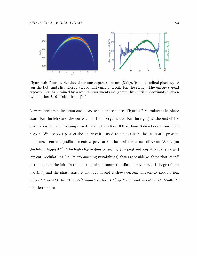
CHAPTER 4. FERMI LINAC 93
Figure 4.6: Characterization of the uncompressed bunch (500 pC): Longitudinal phase space(on the left) and slice energy spread and current pro�le (on the right). The energy spreadreported here is obtained by screen measurements using pure chromatic approximation givenby equation 2.16. Taken from [126].
Now we compress the beam and measure the phase space. Figure 4.7 reproduces the phase
space (on the left) and the current and the energy spread (on the right) at the end of the
linac when the beam is compressed by a factor 5.6 in BC1 without X-band cavity and laser
heater. We see that part of the linear chirp, used to compress the beam, is still present.
The bunch current pro�le presents a peak at the head of the bunch of about 380 A (on
the left in �gure 4.7). The high charge density around this peak induces strong energy and
current modulations (i.e. microbunching instabilities) that are visible as three �hot spots�
in the plot on the left. In this portion of the bunch the slice energy spread is large (about
300 keV ) and the phase space is not regular and it shows current and energy modulation.
This deteriorates the FEL performance in terms of spectrum and intensity, especially at
high harmonics.
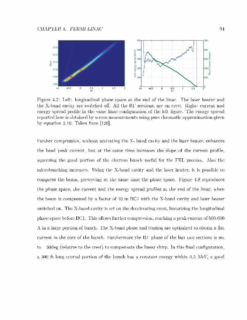
CHAPTER 4. FERMI LINAC 94
Figure 4.7: Left: longitudinal phase space at the end of the linac. The laser heater andthe X-band cavity are switched o�. All the RF sections, are on crest. Right: current andenergy spread pro�le in the same linac con�guration of the left �gure. The energy spreadreported here is obtained by screen measurements using pure chromatic approximation givenby equation 2.16. Taken from [126].
Further compression, without activating the X- band cavity and the laser heater, enhances
the head peak current, but at the same time increases the slope of the current pro�le,
squeezing the good portion of the electron bunch useful for the FEL process. Also the
microbunching increases. Using the X-band cavity and the laser heater, it is possible to
compress the beam, preserving at the same time the phase space. Figure 4.8 reproduces
the phase space, the current and the energy spread pro�les at the end of the linac, when
the beam is compressed by a factor of 10 in BC1 with the X-band cavity and laser heater
switched on. The X-band cavity is set on the decelerating crest, linearizing the longitudinal
phase space before BC1. This allows further compression, reaching a peak current of 500-600
A in a large portion of bunch. The X-band phase and tension are optimized to obtain a �at
current in the core of the bunch. Furthermore the RF phase of the last two sections is set
to +30deg (relative to the crest) to compensate the linear chirp. In this �nal con�guration,
a 300 fs long central portion of the bunch has a constant energy within 0.5 MeV, a good

CHAPTER 4. FERMI LINAC 95
slice energy spread (around 150-200 keV ) and a peak current greater than 600 A.
Figure 4.8: Left: longitudinal phase space at the end of the linac. The laser heater andX-band cavity are on and optimized. All the RF sections, with the exception of the lasttwo are set to +30 deg o� crest. The vertical axis of the plot on the left is scaled to resolvethe residual quadratic chirp. Right: current and energy spread pro�le in the same linaccon�guration of the left �gure. The energy spread reported here is obtained by screenmeasurements using a pure chromatic approximation given by equation 2.16. Taken from[126].
4.4 Design and implementation of a laser heater for FERMI
In this section we describe the laser heater implemented for FERMI [107, 156]. Figure 4.9
is a picture of the laser heater system installed in the linac tunnel.

CHAPTER 4. FERMI LINAC 96
Figure 4.9: Laser heater system installed in the linac tunnel: a) input laser table, b) chicanemagnet, c) multi-screen station LH01.02, d) laser heater undulator; e) multi-screen stationLH01.02, f) BPM LH01.03, g) output laser table. The green arrow shows the direction oflaser and electron beam.
The four dipoles shown in �gure 4.9 form a chicane, shown in �gure 4.10, that creates a
horizontal bump in the beam trajectory. The �rst pair of magnets de�ects the beam on a
line, which is parallel to the linac axis at a distance of 0.03 m from it. Then the electron
beam goes straight for ≈3 m before to be bent, by the second pair of magnets, on the linac
axis. The undulator axis and the path of the laser used to heat the beam are collinear with
the electron beam trajectory in the chicane.

CHAPTER 4. FERMI LINAC 97
Figure 4.10: Electron beam trajectory in the laser heater chicane. The �rst pair of magnetsde�ects the beam on a line, which is parallel to the linac axis at a distance of 0.03 m fromit. Then the beam is de�ected again on the linac axis by the second pair of magnets.
The laser heater undulator is a simple planar permanent magnetic structure. The undulator
parameters have been chosen to be resonant with the wavelength of the laser (783 nm) used
to heat the beam. The electron beam energy at the heater location was not �xed, when the
undulator was designed but was expected in the range from 85 MeV to 105 MeV. Therefore
the undulator was designed to be resonant in this energy window with the wavelength of
the laser. The resonant wavelength is determined by the undulator period, the beam energy
and the K according to equations 1.4-1.5. We can use the following relation between the
K0 and the undulator gap for a planar undulator [24]:
K0 = 160.77 ·Br(T ) · λUe−π·gλU (4.1)
where Br is the remnant �eld characterizing the permanent magnets used to build the
undulator. In our case Br = 1.2T . We calculate, from equations 1.4-1.5 and 4.1, the
beam energy for which the undulator is resonant, at the laser wavelength, as function of
the undulator gap for several values of the undulator period. The result is shown in �gure
4.11 [107].

CHAPTER 4. FERMI LINAC 98
Figure 4.11: Resonance energy in vs. undulator gap. The undulator tunability has beenevaluated for di�erent undulator period lengths.
The undulator period determines the minimum energy at which the undulator is resonant
and the minimum gap needed. In �gure 4.10 we see that the undulator is not resonant at
beam energy of 85 MeV for periods longer than 4.3 cm. We see even that periods shorter
that 3.9 cm require a gap shorter than 20 mm. In this case the height of the vacuum
chamber should be ≤ 18mm. A period 4 cm long has been therefore chosen to allow using
a slightly larger vacuum chamber that was easier to integrate in this part of the machine.
The expected gap operation range is 24-32 mm. The number of periods has to be limited
in order to have a large energy acceptance but large enough to ensure good e�ciency as
the energy spread added by the heater is proportional to the square root of the laser power
and in a �rst approximation, neglecting laser di�raction, linear with the number of periods
as shown in the equation 2.36. The actual number of periods of laser heater undulator is
12. This corresponds to a bandwidth of ≈8%. Simulations have been performed to validate
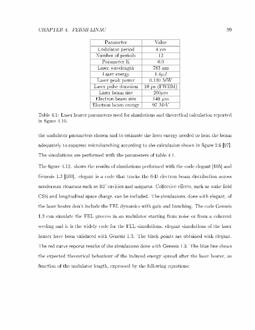
CHAPTER 4. FERMI LINAC 99
Parameter Value
Undulator period 4 cmNumber of periods 12
Parameter K 0.9Laser wavelength 783 nmLaser energy 1.4µJ
Laser peak power 0.130 MWLaser pulse duration 10 ps (FWHM)Laser beam sise 200µm
Electron beam size 140 µmElectron beam energy 97 MeV
Table 4.1: Laser heater parameters used for simulations and theoretical calculation reportedin �gure 4.10.
the undulator parameters chosen and to estimate the laser energy needed to heat the beam
adequately to suppress microbunching according to the calculation shown in �gure 2.6 [97].
The simulations are performed with the parameters of table 4.1.
The �gure 4.12. shows the results of simulations performed with the code elegant [165] and
Genesis 1.3 [160]. elegant is a code that tracks the 6-D electron beam distribution across
accelerator elements such as RF cavities and magnets. Collective e�ects, such as wake �eld
CSR and longitudinal space charge, can be included. The simulations, done with elegant, of
the laser heater don't include the FEL dynamics with gain and bunching. The code Genesis
1.3 can simulate the FEL process in an undulator starting from noise or from a coherent
seeding and it is the widely code for the FEL simulations. elegant simulations of the laser
heater have been validated with Genesis 1.3. The black points are obtained with elegant.
The red curve reports results of the simulations done with Genesis 1.3. The blue line shows
the expected theoretical behaviour of the induced energy spread after the laser heater, as
function of the undulator length, expressed by the following equations:

CHAPTER 4. FERMI LINAC 100
σγ(LU) =√
(σγ0)2 + (σγ(LU))2
Laser heater (4.2)
(σγ(LU))Laser heater =
LU∫0
√σ2r (s)
σ2x + σ2
r (s)
√PLP0
K
σr (s) γ0
JJ(K)ds (4.3)
See section 2.3 for the notation used here. The �rst term of the sum in equation 4.2 is the
initial slice energy spread of the beam coming from the photoinjector. The second term is
the energy spread added by the heater. The integration is on the longitudinal undulator
coordinate. The electron beam dimension is constant to a good approximation along the
undulator. Equations 4.2 and 4.3 are obtained from equations 2.36 and 2.38 and further
modi�ed to take into account the laser di�raction in the undulator. In equations 2.36 and
2.38 any quantity is considered constant along the undulator and the energy spread grows
linearly along the undulator while in equation 4.3 the transverse dimension of the laser
beam changes according to di�raction and integration permits to sum the contributions to
the energy spread at any undulator location.

CHAPTER 4. FERMI LINAC 101
0 0.1 0.2 0.3 0.4 0.53
4
5
6
7
8
9
10
11
Undulator length (m)
Bea
m s
lice
ener
gy s
prea
d af
ter
lase
r he
ater
(ke
V)
Genesis simulationTheoryElegant simulation
Figure 4.12: Behaviour of the energy spread added by the laser heater along the undulator.The red curve reports results of Genesis 1.3 simulation, The blue curve is obtained by theequation. The black points are obtained with elegant. The results of the three methods arein good agreements.
The results of the simulations with the two codes are in good agreements with the theoretical
calculations. The results of simulations and theory shows that the chosen parameters of
the undulator give the required energy spread, needed to suppress microbunching (�gure
2.5), with a small laser energy of ≈1.4 µJ . It is then possible to use a portion of the
photocathode infrared drive laser picked up before the crystal that produces the UV beam
for the photocathode. The FWHM duration of the laser pulse is ≈12 ps and it is close to
be twice the electron beam (≈6.5 ps FWHM). Up to 160 µJ of energy are available for the
heater after the beam transport corresponding to a peak power of ≈16 MW. This level of
laser energy gives a measured energy spread of ≈100 keV ; that is 10 times the optimum one
�xed by simulations and linear theory (�gure 2.5). The laser is transported on an optical

CHAPTER 4. FERMI LINAC 102
table placed in the linac tunnel, near the electron beam vacuum pipe and before the LH
chicane. Two mirrors located on this table steer the laser beam to overlap with the electron
beam trajectory. Another optical table is placed on the other side of the chicane to host
additional diagnostics and the laser dump. Three CCD cameras looking at three screens
permit to have replicas of the beam spot at the two ends of the undulator and at the centre
of the undulator and this allows the laser position and spot size to be monitored. Su�cient
space for two multi-screens, the undulator, the undulator correctors coils and one BPM has
been allocated in the drift between the two pairs of dipoles. The chicane provides a useful
temporal smearing of the laser-induced energy modulation, resulting in a random energy
spread with no temporal structure. This smearing e�ect can be explained by analysing the
beam dynamics in the second half of the laser heater chicane with the matrix formalism
introduced in section 2.1. The longitudinal bunch coordinate (i.e., referred to the beam
centre of mass) of a particle in a point f is related to the position at a starting point i,
located just after the undulator, through the following �rst order equation:
z(f) = z(i) +R51x(i) +R52x′(i) +R56
∆L(r)sin (kLz(i))
γ0
(4.4)
All the quantities appearing in equation 4.4 were de�ned in section 2.1 and 2.3. For a
symmetric achromatic chicane the relevant coe�cients across the half-chicane are R51 = 0
and R52 = −η where η is the dispersion in the middle of the chicane and it is equal in a
�rst approximation to the displacement between the linac axis and the beam trajectory in
the middle of the chicane. This gives, η≈− 0.03m in the centre of the laser heater chicane.

CHAPTER 4. FERMI LINAC 103
The smearing of the time-energy correlation (2.30) occurs because the path length from
the chicane centre, where the energy modulation is induced, to the chicane end depends on
the electron's x' coordinate across the non-zero chicane transport element R52 introduced
in section 2.1. Particles, with di�erent x' of a �nite emittance beam (ε 6= 0), move on
di�erent paths across the second half chicane. At coordinate i there is no x'-z correlation
and at any longitudinal coordinate z there is an angular spread due to �nite emittance.
Particles at an initial longitudinal coordinate z(i), with di�erent x', are spread on a slice of
the bunch with an RMS length of R52σ′x. The smearing of time-energy correlation (2.30),
with the characteristic wavelength scale given by the radiation wavelength λL, occurs if the
condition R52σ′x > λL/2π is satis�ed. Where σ
′x =
√εxβx
is the beam angular spread at the
centre of the chicane. The angular dispersion at the centre of the chicane is 37µm and the
dispersion is 30mm for the FERMI case. So all the modulations with a reduced period much
shorter than ≈1 µm are smeared while the reduced wavelength for the laser modulation is
(λ/2π = 126nm). The laser heater energy modulation takes place in a dispersive region
such that in principle it can produce a beam emittance growth. The laser energy modulation
produces a growth of the longitudinal phase space area occupied by the beam dynamics as
the energy spread is increased. The chicane dispersion couples the longitudinal dynamics
to the transverse dynamics as the beam goes from the undulator's axis to the linac axis (see
�gure 4.10). So the area occupied by the beam in the transverse plane, i.e. the transverse
emittance, is increased. The horizontal beam dimension after the chicane is:
σx =
√(σx)
2Twiss +
(η · (σγ)Laser heater
γ
)2
= (σx)Twiss
√1 +
(η · (σγ)Laser heaterγ · (σx)Twiss
)2
(4.5)

CHAPTER 4. FERMI LINAC 104
Taking the values of the parameters in table 4.1 and a dispersion η ≈ 0.03m we obtain an
increase in the beam dimension of 0.01% due to laser heater energy modulation and chicane
dispersion. This level of emittance dilution is very small and completely acceptable. Two
screen diagnostic stations, one on each side of the undulator, lie within the LH chicane. Both
diagnostic stations are equipped with Cromox (Al2O3:Cr) screens on which it is possible to
image both the laser and the electron beam in order to superimpose them transversely.
4.5 Commissioning of the FERMI laser heater
At the begin of laser heater commissioning the laser central wavelength had to be matched
with that of the undulator spontaneous radiation and the electrons and laser beam had to
been aligned transversely and superimposed longitudinally in the laser heater undulator.
The relative bandwidth of undulator radiation is ≈8%, while the electron beam energy
is known with an error of less than 1% and the undulator magnetic �eld, at which the
parameter K is proportional, is measured with at error of 0.3%. Therefore it is very easy to
�nd the resonance with an acceptable accuracy, as the reduction of induced energy spread
due to these errors is less than 10% as can be seen in �gure 4.21. The mechanic undulator
gap control, allows the vertical position of the undulator axis to be changed to centre the
undulator axis on the beam. We have then aligned vertically the axis of the undulator on
the beam trajectory looking at the trajectory downstream both with undulator open and
with undulator closed. Since both the electron beam and the external laser originate from
the photocathode infrared drive laser, they are naturally locked in time but with a constant
temporal o�set: After the beam splitter that takes out the portion of laser used to heat the

CHAPTER 4. FERMI LINAC 105
beam, they follow two di�erent paths to meet again after about 20 m. This temporal o�set
can be measured with an accuracy of about 300 ps, by recording with an oscilloscope the
signal coming from a photodiode located at the LH input laser table and a signal of one
beam position monitor (BPM) located near the chicane. The �ne temporal overlap is then
found by scanning a delay line to superimpose the two beams temporally, while checking the
beam heating on the beam spectrometer as we will see later. Three remotely controllable
mirrors, one in the laser room and two on the optical table at the chicane entrance, permit
the adjustment of the laser centroid position relative to that of the electrons with 100 mm
accuracy, as shown in �gure 4.13. The laser transverse pro�le imaged on the two screens at
both the ends of the undulator is shown on the left while on the right we can see the two
images of the electron beam.
The BPM placed in the chicane allows any change in the electron beam energy to be
monitored. When the electron beam and the laser beam are aligned in space and time,
the laser-electron interaction in the undulator generates signi�cant energy spread that is
easily detected using the spectrometer placed after the �rst bunch compressor (�gure 3.2).
The beam is de�ected vertically with a vertical RF de�ector [126-128] before entering into
the spectrometer. The magnetic lattice produces a momentum-dispersion h ≈0.58 m and
a betatron function b ≈1 m at the YAG screen location. On the screen placed after the
spectrometer dipole it is possible to reconstruct the beam longitudinal phase space, so
enabling the measurement of the uncorrelated energy spread in each longitudinal slice of the
bunch. Figure 4.14 shows a representative longitudinal phase space when the LH is switched
o� (left) and when the beam is heated (right), at full energy (160 mJ). The minimum slice
energy spread, measured in pure chromatic approximation (equation 2.16) when the LH was

CHAPTER 4. FERMI LINAC 106
Figure 4.13: Image of laser (a and b) and electron beam (c and d) on two CROMOX screentargets at the undulator entrance (a and c) and exit (b and d). The red cross indicates thecentre of the screen.

CHAPTER 4. FERMI LINAC 107
Figure 4.14: Longitudinal electron beam phase space reconstructed on the spectrometerscreen with the RF de�ector on. The left image is taken with the laser heater o�. The rightimage shows the beam phase space with the heater on with a laser energy of 160 µJ.
o�, is ≈40 keV. The nominal lattice geometry resolution is ≈20 keV, the screen resolution
gives ≈20 keV and de�ector adds ≈28 keV [129]. The transverse RMS dimension of the
laser beam in the undulator is around ≈200 µm, while the electron beam size is ≈140 µm.
The heated beam is expected to show a double horn energy distribution [95, 107] when
the laser transverse pro�le is larger than the electron beam, as shown in �gure 2.4. The
energy distribution is more Gaussian-like when the laser matches the electron beam size in
the undulator. This con�guration has been shown to be more e�ective in suppressing the
microbunching instability [95] as seen in section 2.3. In spite of this, we started with a large
laser spot to more easily overlap the electron and the laser beam.
Figure 4.15 shows the longitudinal behaviour of the slice energy spread along the beam

CHAPTER 4. FERMI LINAC 108
0 2 4 6 8 10 120
20
40
60
80
100
120
140
160
180
Bunch longitudinal position (ps)
Ene
rgy
spre
ad (
keV
)
Measured energy spread (heater on)Measured energy spread (heater off)Heated beam energy spread (measured)Heated beam energy spread (elegant simulation)
Figure 4.15: Slice energy spread along the longitudinal beam pro�le. The green curve showsthe energy spread measured with the LH o�, the red curve reproduces the energy spreadof the beam heated at the maximum laser energy of 160 µJ and the blue curve is obtainedsubtracting in quadrature the green curve from the red one. The magenta line shows theslice energy spread along the longitudinal electron beam pro�le obtained with elegant.
pro�le. The green curve shows the energy spread measured with the LH o�, the red curve
reproduces the energy spread of the beam heated at the maximum laser energy of 160 µJ.
The blue curve is the LH induced energy spread only, obtained by subtraction in quadrature
of the �rst two. We see that the variation of the beam heating is about 20% on a central
portion of the beam with a duration of ≈7 ps. This seems a good uniformity of the beam
heating on the region of the beam on which the FEL pulse is produced. The magenta line
shows the energy spread slice pro�le as obtained from an elegant simulation. It is again in
good agreement with the experimental result (blue curve).
Figure 4.16 shows the evolution of the energy spread of a central slice of the beam as
a function of the laser energy. The values shown by the blue experimental points are
obtained by subtracting in quadrature the energy spread measured with LH o� from the
value measured with LH on. Doing so, one ideally obtains the energy spread added by the

CHAPTER 4. FERMI LINAC 109
laser heater only. The magenta line shows the expected theoretical behaviour (equation
4.3). The error bars are obtained from statistical measurement errors on 15 shots.
−20 0 20 40 60 80 100 120 140 160 180−20
0
20
40
60
80
100
120
Laser heater (µJoule)
Add
ed e
nerg
y sp
read
(\k
eV)
Figure 4.16: Laser heater added slice energy spread vs. laser energy.
Figure 4.16 shows a good agreement between theory and the measured data. The measure-
ments reported above are taken with the gap optimized for the maximum beam heating.
In �gure 4.17 we show the behaviour of the added energy spread with a laser energy of
160 µJ as a function of the undulator gap. The blue curve shows the theoretical expected
behaviour. The green points in �gure 4.17 with the error bars are the measured values of
the energy spread, added by the laser heater to a central slice, for several values of the
undulator gap. The blue curve reproduces the theoretical behaviour of the energy spread,
that is proportional to the sinc function of the detuning between the laser wavelength and

CHAPTER 4. FERMI LINAC 110
the undulator resonance wavelength [32, 33], as a function of K (see equations 1.4-1.5):
σγ (g) = σγ (gL)
∣∣∣∣∣∣sin{πN [λ(g)−λL]
λL
}πN [λ(g)−λL]
λL
∣∣∣∣∣∣ (4.6)
λ (g) = 〈λθ (g)〉θ (4.7)
〈λθ (g)〉θ =
{λU2γ2
0
[1 +
K (g)2
2
]}+εnγ0
β
(λU2γ2
0
)(4.8)
Here g is the undulator gap, εn is the normalized beam emittance and β is the average
betatron function in the undulator. Equation 4.6 is valid for a beam propagating along
the undulator axis without an angle. In reality, every particle has an angular divergence
with respect to the straight reference axis, due to the beam �nite emittance. The mean
resonance frequency λ (g) is then obtained mediating on the beam angular divergence and
is shifted with respect to the case of a 1-D beam, by a term determined by the emittance
and the betatron function in the undulator. This shift is the second term in 4.6. The beam
in the LH has a normalized emittance ≈1 mm·mrad, and β≈2.5 m. The wavelength shift
due to the �nite emittance is then <0.01% of the wavelength resonance for a zero emittance
beam. The magenta line in �gure 4.17 is obtained by shifting the blue curve to match the
experimental points. This shift corresponds to an electron beam energy of 97.2MeV instead
of 97.7 MeV. This shift is compatible with the expected error of the undulator calibration
curve and of beam mean energy error measurement.
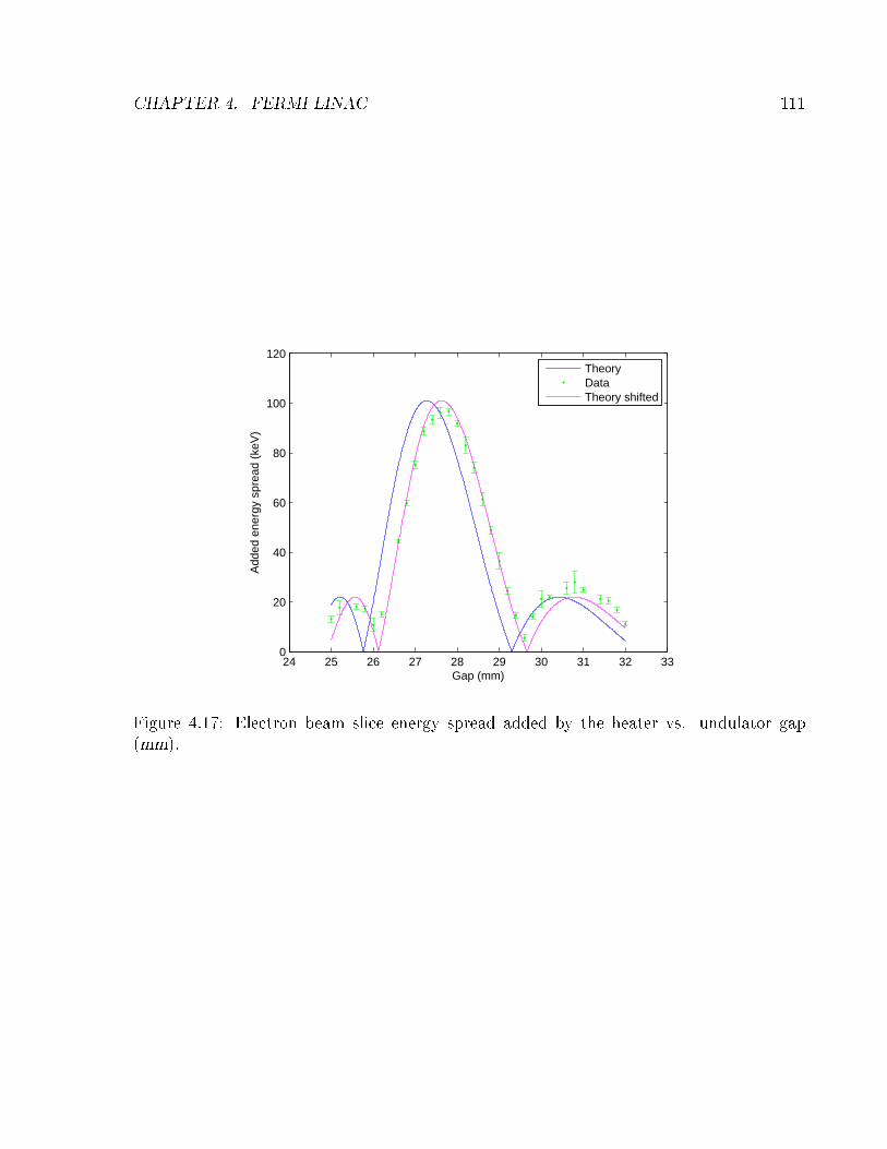
CHAPTER 4. FERMI LINAC 111
24 25 26 27 28 29 30 31 32 330
20
40
60
80
100
120
Gap (mm)
Add
ed e
nerg
y sp
read
(ke
V)
TheoryDataTheory shifted
Figure 4.17: Electron beam slice energy spread added by the heater vs. undulator gap(mm).

CHAPTER 4. FERMI LINAC 112
4.6 Microbunching suppression
Now we analyse the e�ect of the LH on the electron beam dynamics downstream of the
compressor. Clear evidence of microbunching instability e�ects can be seen when the linac
is set to a compression factor greater than 3 as both the current and energy spectrum of the
beam appear to be modulated. Figure 4.18 shows the electron beam energy pro�les imaged
on the screen of the spectrometer line in the diagnostic beam dump (DBD in �gure 3.5),
placed at the end of the linac.
Figure 4.18: Beam energy pro�les imaged on the screen of the spectrometer in the diagnosticbean dump (DBD) for three levels of beam heating. a: 0 heating. b: 4.5 keV heating. c:15 keV heating.
These data were acquired for a 500 pC beam charge with a compression factor of about 5.5
using only BC1. The X-band RF cavity (so-called linearizer) upstream of BC1 was switched
o� so that a non-linear magnetic compression produced a triangular current distribution.
The magenta curve in �gure 4.18a displays the energy pro�le measured with the LH switched
o�. It shows high frequency modulations that we attribute to the microbunching instability,

CHAPTER 4. FERMI LINAC 113
together with a longer time-scale structure produced by non-linearities during the magnetic
compression. When the LH is turned on with a laser energy of ≈0.25 µJ, the high frequency
structures start to be reduced in amplitude (�gure 4.18b), whereas the macroscopic current
structures were almost untouched by this small level of heating. When the laser energy was
increased to a level of ≈2 µJ or greater, even the longer scale structures were smeared out,
as shown in �gure 4.18c.
The suppression of the phase space modulation, seen as a smoothing of the beam energy
spectrum in �gure 4.18, can be seen clearly by de�ecting the beam with the vertical de�ector
and then bending it with a horizontal dipole magnet [164]. Figure 4.19 shows the beam
phase space imaged on the spectrometer screen. We see, on the left of the picture, that the
LH suppresses the microbunching structures located at the head of the beam.

CHAPTER 4. FERMI LINAC 114
Figure 4.19: Beam longitudinal phase space at the linac end. Top: no LH and no X-bandcavity, all RF sections on crest, 500 pC . Bottom: LH on but without X-band cavity, all RFsections on crest, 500 pC . Taken from [126].
Further evidence of microbunching instability gain is the coherent optical transition radia-
tion (COTR) produced when the beam passes through OTR target screens [130, 166, 167].
The LH reduces and eventually suppresses these COTR signals. Figure 4.20 shows the OTR
signal from screen SFEL01.02 placed just upstream of the FEL1 undulator as a function
of LH energy. One sees a strong suppression of the signal for laser energies exceeding 1
µJ. The data reproduced here are taken with 350 pC charge, a compression factor close
to 10 and the X-band cavity switched on to have a more regular �nal current pro�le. The
beam is compressed using only BC1. The COTR from SFEL01.02 is strongly suppressed,

CHAPTER 4. FERMI LINAC 115
with a charge of 500 pC and a compression factor of 10. The signal, from this screen, can
sometimes remain 10%-20% higher with respect to the incoherent level if CSR, microbunch-
ing and dispersive e�ect are not completely controlled in the spreader [97]. This level of
coherent radiation however corresponds to a very small persistent microbunching.
4 6 8 10 12 14 16 18 20 22 240
0.5
1
1.5
2
2.5
3
3.5
4
4.5x 10
4
Laser heater energy spread (keV)
CC
D in
tens
ity (
arbi
trar
y un
its)
Figure 4.20: OTR intensity vs. laser heater energy.
The intensity decays as the laser energy is increased and approaches a constant level when
the laser energy is above 1.0 µJ. This constant intensity is equal to the incoherent level
obtained by inserting an upstream OTR screen on the beam path. We therefore conclude
that the LH can suppress almost completely, in this linac con�guration, the COTR produced
on this screen when the laser energy is >1.0 µJ. More precisely, by adding an uncorrelated
energy spread larger than 8 keV RMS, one removes completely any beam modulations
detected by the CCD (within the wavelength range 0.2 µm - 0.9 µm). We then increased
the beam charge to 500 pC, keeping unchanged the remaining linac setting and we studied
the e�ect of the LH on the intensity of the OTR radiation produced by the third screen
placed on the straight line after BC01. Figure 4.21 depicts the intensity of the signal
collected by a CCD that looks to this OTR screen.
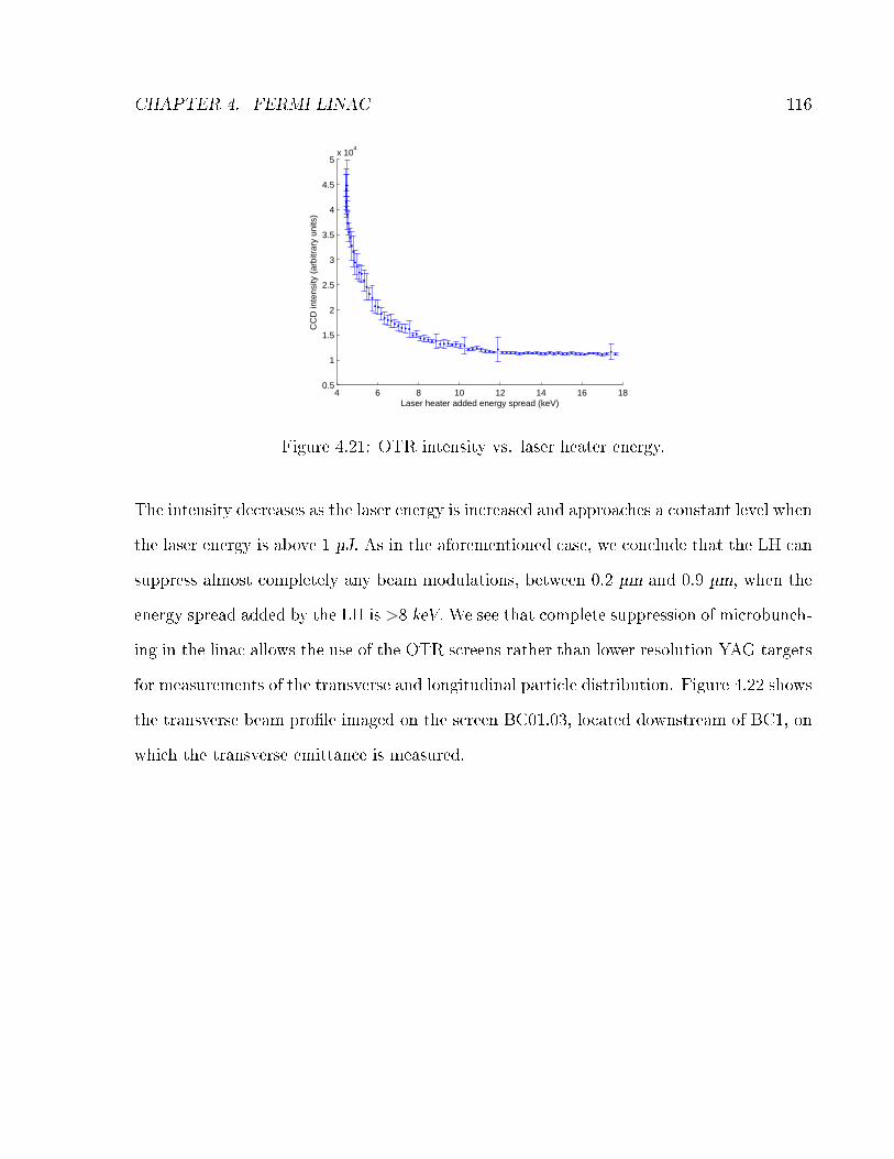
CHAPTER 4. FERMI LINAC 116
4 6 8 10 12 14 16 180.5
1
1.5
2
2.5
3
3.5
4
4.5
5x 10
4
Laser heater added energy spread (keV)
CC
D in
tens
ity (
arbi
trar
y un
its)
Figure 4.21: OTR intensity vs. laser heater energy.
The intensity decreases as the laser energy is increased and approaches a constant level when
the laser energy is above 1 µJ. As in the aforementioned case, we conclude that the LH can
suppress almost completely any beam modulations, between 0.2 µm and 0.9 µm, when the
energy spread added by the LH is >8 keV. We see that complete suppression of microbunch-
ing in the linac allows the use of the OTR screens rather than lower resolution YAG targets
for measurements of the transverse and longitudinal particle distribution. Figure 4.22 shows
the transverse beam pro�le imaged on the screen BC01.03, located downstream of BC1, on
which the transverse emittance is measured.

CHAPTER 4. FERMI LINAC 117
Figure 4.22: Transverse beam pro�le imaged on the screen BC01.03, respectively with LHo� (left) and on (right). Picture from [162].
All the measurements reported above, about the laser heater and microbunching suppres-
sion, were performed with a laser spot larger than the electron beam. After this �rst
operations the laser spot was reduced to about 130µm to better match the electron beam
producing a more homogeneous energy distribution. This is more useful in suppressing the
microbunching but it makes more di�cult to get and maintain the overlap between the
electron and the laser beam. The �gure 4.23 shows the characterization of the laser heater
with the laser matched to the electron beam.
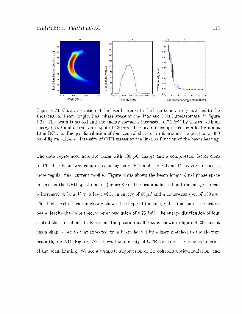
CHAPTER 4. FERMI LINAC 118
Figure 4.23: Characterization of the laser heater with the laser transversely matched to theelectrons. a: Beam longitudinal phase space at the linac end (DBD spectrometer in �gure3.2). The beam is heated and the energy spread is increased to 75 keV by a laser with anenergy 65µJ and a transverse spot of 130µm. The beam is compressed by a factor about10 in BC1. b: Energy distribution of four central slices of 75 fs around the position at 0.9ps of �gure 4.23a. c: Intensity of OTR screen at the linac as function of the beam heating.
The data reproduced here are taken with 500 pC charge and a compression factor close
to 10. The beam was compressed using only BC1 and the X-band RF cavity to have a
more regular �nal current pro�le. Figure 4.23a shows the beam longitudinal phase space
imaged on the DBD spectrometer (�gure 3.2). The beam is heated and the energy spread
is increased to 75 keV by a laser with an energy of 65µJ and a transverse spot of 130µm.
This high level of heating clearly shows the shape of the energy distribution of the heated
beam despite the �nite spectrometer resolution of ≈75 keV. The energy distribution of four
central slices of about 15 fs around the position at 0.9 ps is shown in �gure 4.23b and it
has a shape close to that expected for a beam heated by a laser matched to the electron
beam (�gure 2.4). Figure 4.23c shows the intensity of OTR screen at the linac as function
of the beam heating. We see a complete suppression of the coherent optical radiation, and

CHAPTER 4. FERMI LINAC 119
of the density modulation, at the wavelengths visible to the CCD, 0.2-0.9 nm, for a heating
higher than 8 keV. All these measurements show that this laser heater setting is working
well despite the practical di�culties to take and keep a good alignment, between the laser
and the electron beam, with a so tight laser spot. This spot size has been maintained for
the last measurements shown in this chapter, for the FEL measurement shown in the next
chapter and during FEL user operations. We measure the beam slice energy spread in
the diagnostic area placed at the linac end (�gure 3.2). We have done measurements of the
�nal slice energy spread while compressing the beam with only the �rst compressor and even
with both compressors. The single compressor scheme permits to obtain a smaller value
of slice energy spread with respect to the double compressor scheme and this con�rms the
theoretical and numerical calculation reported in section 2.3. A minimum slice energy spread
of about 100 keV has been measured, in the single compression scheme, for a compression
factor of 10-12 and with an energy spread added by the heater <10 keV [168]. In this
con�guration the expected minimum (�gure 2.6) of the �nal energy spread versus the added
energy spread was not seen during measurements due to the �nite experimental resolution.
We will see in the next chapter that the FEL output power is maximized for a proper value
of the beam heating revealing, probably, a minimum of the slice energy spread. On the
other hand the microbunching is stronger in the double compression scheme and, for this
reason, the minimum of the �nal energy spread obtained for the proper value of heating
is more visible. Figure 4.25 shows the beam slice energy spread as function of the energy
spread added by the heater in the double compressor con�guration. Each energy spread
value is the mean of seven measurements. The expected spectrometer resolution is ≈50 keV ;
another contribution of 50 keV to the measured energy spread is expected by the de�ector
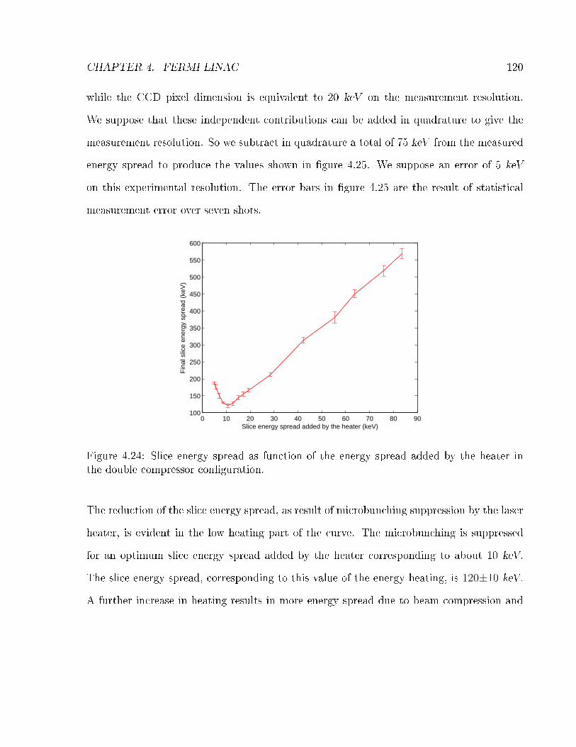
CHAPTER 4. FERMI LINAC 120
while the CCD pixel dimension is equivalent to 20 keV on the measurement resolution.
We suppose that these independent contributions can be added in quadrature to give the
measurement resolution. So we subtract in quadrature a total of 75 keV from the measured
energy spread to produce the values shown in �gure 4.25. We suppose an error of 5 keV
on this experimental resolution. The error bars in �gure 4.25 are the result of statistical
measurement error over seven shots.
0 10 20 30 40 50 60 70 80 90100
150
200
250
300
350
400
450
500
550
600
Slice energy spread added by the heater (keV)
Fin
al s
lice
ener
gy s
prea
d (k
eV)
Figure 4.24: Slice energy spread as function of the energy spread added by the heater inthe double compressor con�guration.
The reduction of the slice energy spread, as result of microbunching suppression by the laser
heater, is evident in the low heating part of the curve. The microbunching is suppressed
for an optimum slice energy spread added by the heater corresponding to about 10 keV.
The slice energy spread, corresponding to this value of the energy heating, is 120±10 keV.
A further increase in heating results in more energy spread due to beam compression and

CHAPTER 4. FERMI LINAC 121
phase space conservation. The measurements taken at high values of added slice energy
spread are less a�ected by the measurement errors and by the initial beam energy spread.
The measured energy spread, at high values of beam heating, is the result of the compression
of the heated beam. From the last six points appearing in �gure 4.24 it is possible to derive
a compression factor of about 7. This is in good agreement with the current measured in
the linac condition at the moment of data collection. In fact we measured an initial current
of ≈60 A and a compressed current of ≈400 A.
In conclusion we have shown that it is possible to control the microbunching instability in
the FERMI linac using the laser heater. A reduction of density and energy modulation due
to the laser has been observed as well as a reduction of the slice energy spread.

CHAPTER 4. FERMI LINAC 122

Chapter 5
FERMI FEL1 commissioning
Here we report a detailed characterization of recent results obtained with FEL1. The X-band
cavity and the laser heater were not available during the �rst year of FEL commissioning.
The compression is non-linear without the X-band cavity and this lead to a current ramp
distribution. During this �rst period the beam compression factor used was around 5.6. The
clean longitudinal phase space allows a very good control of the FEL bandwidth, however
the low current used in this period implies a quite low photon �ux. With the use of the
X-band cavity and of the laser heater it has been possible to increase the beam current and
thus the photon �ux. By following the evolution of the FEL performance in terms of the
spectrum and FEL power it is possible to study the in�uence of the phase space on the
FEL characteristics. We have observed that the ramped current distribution obtained by
gently compressing the 500 pC bunch in the absence of the X-band cavity and of the laser
heater allows a clean, narrow and stable spectrum but a mild-low photon �ux. Increasing
the compression factor to 10-13 with the laser heater and the X-band cavity preserves the
123

CHAPTER 5. FERMI FEL1 COMMISSIONING 124
beam quality while giving a increase in the pulse energy (almost a factor 10-15) preserving
the spectral quality.
5.1 High-gain harmonic generation
The harmonic radiation produced in the FEL process reaches a power level considerably
lower than that of the fundamental component which decreases as the harmonic number
increases [37]. A more e�cient scheme to produce coherent radiation at the harmonics
of the seed can be realized using two undulators with the �rst undulator, the modulator,
tuned to the same wavelength of the external laser and the second one, the radiator, tuned
to the selected harmonic of the seed. A dispersive section, in which particles with di�erent
energy travel along di�erent paths is placed between the two undulators. The energy of the
particles at the end of the �rst undulator is correlated with the phase of the electromagnetic
�eld of the laser, because the sign of the energy exchange due to the Lorentz force depends
on this phase, and with the electron position within the bunch. The interaction between
the external laser and the electron beam in the �rst undulator produces a sinusoidal energy
modulation with the period of the seed laser and a modulation amplitude as described
in section 2.3. The magnetic �eld of the dispersive section forces electrons with di�erent
energies to follow di�erent paths. Therefore, the beam energy modulation with the spatial
period equal to the wavelength of the seed laser is converted into a density modulation.
The Fourier analysis of the beam current shows that components at the harmonics of the
seed are present. The bunching factor at any harmonic of the wavelength of the seed laser
has, at the exit of the dispersive section, the following expression:
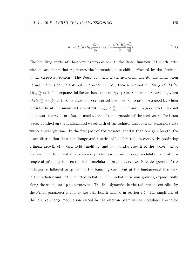
CHAPTER 5. FERMI FEL1 COMMISSIONING 125
bn = Jn(nkR564γγ0
) · exp(−n2k2R2
56
2
σ2γ
γ20
) (5.1)
The bunching at the nth harmonic is proportional to the Bessel function of the nth order
with an argument that represents the harmonic phase shift performed by the electrons
in the dispersive section. The Bessel function of the nth order has its maximum when
its argument is comparable with its order number, then a relevant bunching comes for
kR564Lγ0≈ 1. The exponential factor shows that energy spread reduces microbunching when
nkR56σγγ0≈ n σγ
4L> 1, so for a given energy spread it is possible to produce a good bunching
down to the nth harmonic of the seed with nmax <4γσγ. The beam thus goes into the second
undulator, the radiator, that is tuned to one of the harmonics of the seed laser. The beam
is just bunched on the fundamental wavelength of the radiator and coherent emission starts
without lethargy time. In the �rst part of the radiator, shorter than one gain length, the
beam distribution does not change and a series of bunches radiate coherently producing
a linear growth of electric �eld amplitude and a quadratic growth of the power. After
one gain length the radiation emission produces a relevant energy modulation and after a
couple of gain lengths even the beam modulation begins to evolve. Now the growth of the
radiation is followed by growth in the bunching coe�cient at the fundamental harmonic
of the radiator and of the emitted radiation. The radiation is now growing exponentially
along the undulator up to saturation. The �eld dynamics in the radiator is controlled by
the Pierce parameter ρ and by the gain length de�ned in section 2.4. The amplitude of
the relative energy modulation gained by the electron beam in the modulator has to be

CHAPTER 5. FERMI FEL1 COMMISSIONING 126
smaller than the Pierce parameter of the radiator otherwise many particles fall outside of
the resonance too early and the FEL interaction is reduced. The limitation on the harmonic
order that can be reached becomes nmax <σσγ
and the energy modulation induced in the
modulator has to be in the range of nσγ < 4γ < σ where n is the harmonic number to which
the radiator is tuned. A bunching of few per cent, on the harmonic to which the radiator
is tuned, is enough to overcome the shot noise and ensure an increase of the radiation in
the second undulator. Another stage with a modulator a dispersive section and a radiator,
using the radiation coming from the �rst radiator as seed, can follow the �rst one. The
radiation production in the �rst stage can decrease the beam quality increasing the slice
energy spread. This unwanted phenomenon occurs mainly on the part of the beam that
interacted with the seed in the �rst stage as seeded FEL can be optimized to evolve faster
than SASE. Then it is enough to add a delay line for the electron beam, between the two
stages to put the seed produced in the �rst stage on a fresh part of the electron bunch. This
technique is called fresh bunch and it will be explored for the �rst time on FERMI's FEL2
line.
5.2 Low compression scenario
For the FEL1 experiments reported in this section the seed laser was the third harmonic
(260 nm) of the Ti:Sa laser. The seed laser pulses had a duration of 150 fs (FWHM), a
peak power of about 100 MW and a bandwidth of about 0.8 nm, which is about a factor
1.2 larger than the Fourier limit, assuming perfectly Gaussian pulses. The electron beam
had a charge of 450-500 pC and was compressed by a factor 3-4 in BC01, without the

CHAPTER 5. FERMI FEL1 COMMISSIONING 127
Parameter Value
Energy 1.24 GeVSlice energy spread (RMS) <150 keVEmittance (projected ) ∼ 4 mm· mrad
Charge 400 pCPeak current 200-300 ABeam size 150 µm
Pierce parameter 1.3 10−3
Table 5.1: Measured electron-beam parameters used to operate FEL1 in the experimentsreported in this paragraph.
X-band cavity and the laser heater. The measured values of electron-beam parameters used
to operate FEL1 in the reported experiments are listed in the table 5.1
The beam phase space is shown in �gure 4.7. The temporal coarse alignment and spatial
alignment were done, as described in section 3.1, before establishing seeding operation. The
dispersive section was switched on to a value of 50− 70µm, the gap of the modulator and
of the radiator were tuned respectively to the nominal value for the seed wavelength (the
modulator) and of the desired harmonic (the radiator). Then, the seeded FEL was switched
on by scanning the delay line. Figure 5.2 shows the FEL output energy versus the seed
delay. This scan gives an indication of the temporal duration and shape of the electron
beam region involved in the photons production. We will see later that it is possible to
demonstrate that the interaction happens in the tail of the bunch for positive delays in
�gure 5.1 and in the head for negative delays.

CHAPTER 5. FERMI FEL1 COMMISSIONING 128
−0.6 −0.4 −0.2 0 0.2 0.4 0.6 0.8 1 1.2−2
0
2
4
6
8
10
12
14
16
Delay (ps)
Ioni
zatio
n M
onito
r C
urre
nt (
pC)
Figure 5.1: Seed delay scan. The temporal delay between the seed and the electron beamis scanned while recording the FEL intensity on a diode. In this way it is possible �nd theperfect time overlap between the two beams.
The curve reproducing the FEL intensity vs. the seed delay is asymmetric and inherits the
principal characteristic from the beam current (green curve) and energy spread pro�le (blue
curve) shown in �gure 4.7. The FEL energy, as the seed is moved from the tail to head,
increases almost proportionally with the square of the beam current. The growth of the
FEL power stops before the current peak shown in �gure 4.7 (green curve) as this part of
the beam is spoiled by the microbunching that increases the energy spread and modulates
the phase space as can be seen in �gure 4.7. The FEL energy goes down rather quickly with
the current. The full width half maximum (FWHM) duration of the curve in �gure 5.1 is
about 300 fs and this can be considered as the temporal duration of the part of the beam
that �ts the requirements of FEL.
We obtained several tens of microjoules of FEL emission from the fourth harmonic of the

CHAPTER 5. FERMI FEL1 COMMISSIONING 129
seed down to the thirteenth harmonic (20 nm) in the range speci�ed for FEL1. Figure
5.2 highlights the transverse and longitudinal quality of the radiation at 20 nm. The FEL
spot, imaged on a YAG screen placed at about 52.4m downstream of the last undulator,
is reproduced in �gure 5.2a. The RMS transverse size is about 1.4 mm in both planes and
this is in good agreement with expectations for a Gaussian beam with a beam waist at the
exit of the last undulator of 200 µm consistent with the electron beam size at that point.
Figure 5.2b shows a single-shot spectrum at 20 nm. The bandwidth (FWHM) is ≈0.009
nm and this gives a time-bandwidth product of about 0.56 that is ≈1.3 times the one for a
Gaussian beam and this indicates the good longitudinal coherence of the FEL.
Figure 5.2: Transverse and spectral characterization of the radiation at 20 nm. a) Image ofthe radiation at 20 nm on a YAG screen placed at ≈ 52.4m downstream of the radiator.b) Single-shot spectrum of the radiation at 20 nm. Courtesy of E. Allaria.
Clear evidence of coherent emission was observed at the �fteenth harmonic (17 nm) exceed-
ing the harmonic conversion factor �xed for FEL1. This indicates a very bright electron
beam. For each harmonic, the FEL has been optimized by tuning the amplitude of energy
modulation produced in the modulator (controlling the seed power) and the strength of

CHAPTER 5. FERMI FEL1 COMMISSIONING 130
the dispersive section. The optimization procedure generally leads to a setting with a R56
in the range between 40 and 70µm. A complete characterization of the light produced at
the eighth harmonic of the seed laser (32.5 nm) is reported in the following. We obtained
similar results in the whole spectral range between 26 and 65 nm. After optimization of
the FEL process to maximize the output energy from the whole radiator (6 sections) tuned
at 32.5 nm, we measured the energy, with the photodiode and the layout shown in �gure
3.10 [127], as a function of the number of sections contributing to the coherent emission.
The FEL power has been estimated from the pulse energy, considering that the simulations
predict for these conditions an FEL pulse of about 85 fs FWHM. Figure 5.3a shows the
measured FEL power evolution along the FEL1 radiator, for both planar and helical undu-
lator con�gurations. In the inset, the same data are reported on a logarithmic scale, clearly
showing the di�erent gain lengths associated with the two polarizations. Fitting the data
with an exponential curve yields a gain length (de�ned in sections 1.2 and 2.4) of about
2.5 meters for planar polarization and 2.0 meters for circular polarization. This result is
in good agreement with both the gain length calculated using the FEL parameter and the
formula by Ming Xie [55] evaluated with the electron beam parameter reported in table
5.1. As expected, in the case of circular polarization, a shorter gain length and a higher
output power is obtained due to better coupling between the electromagnetic �eld and the
electrons, compared to the case of linear polarization. The measured FEL evolution is also
in good agreement with the numerical simulation performed using the GINGER numeri-
cal code. Figure 4.1a reports the predicted output power obtained by simulations. The
measurement of the gain length is not a�ected by the absolute calibration of the detector,
as that of the pulse energy. So performing these measurements it is possible to validate,

CHAPTER 5. FERMI FEL1 COMMISSIONING 131
with good precision, the expected brightness of the electron beam. The agreement of the
actual FEL growth with the expected one allows even to state that the electrons-radiation
coupling along the radiator is not much spoiled by an imperfect tuning of the undulator
and by imperfections of the electron beam trajectory. It is worth noting that FERMI FEL
achieved a power close to the level of SASE saturation with a radiator that is about 6-8
gain lengths, while for a SASE FEL generally about 20 gain lengths are needed. The SASE
process (sections 1.2 and 2.4) starts from a very low bunching (0.01%-0.05%) while typically
in HGHG scheme a bunching of a few per cent (1%-5%), produced in the dispersive section,
drives the growth of FEL radiation in the radiator. Then SASE process needs a longer
undulator to reach the same power level compared to HGHG.

CHAPTER 5. FERMI FEL1 COMMISSIONING 132
Figure 5.3: Measured FEL intensity at 32.5 nm. a: Measured FEL energy per pulse (sym-bols, right axis) as a function of the number of undulator sections used in the radiator,and predicted FEL power from numerical simulations [37] (lines, left axis). Data are shownfor both circular (red symbols) and horizontal (blue symbols) polarization of the radia-tor sections. Error bars re�ect the statistical distribution of results obtained from severalconsecutive pulses. In the inset, the same data are reported in a logarithmic scale. b:Typical shot-to-shot distribution of the pulse energy per for 500 consecutive FEL pulses.The quasi-Gaussian distribution characterized by a standard deviation of about 10% re�ectsshot-to-shot �uctuations in the electron-beam parameters. Taken from [13].
Moreover as shown in �gure 4.1b, the measured FEL energy �uctuations are of the order
of 10%, following an approximately Gaussian distribution. These results show how the
use of an external seed allows us to keep the power �uctuations under control, without
the need to enter deeply into the saturation regime, as is necessary in the case of SASE.
Since it has been predicted that some of the desirable FEL properties, such as transverse
and longitudinal coherence, can be degraded when a SASE FEL is operated in the satura-
tion regime SASE FELs may require operation under conditions that strike a compromise

CHAPTER 5. FERMI FEL1 COMMISSIONING 133
between maximum output power, reduced �uctuations and high coherence. This compro-
mise has been demonstrated to be less critical for FERMI where these properties can be
controlled simultaneously. It is also important to point out the di�erent origins of power
�uctuations in SASE and HGHG FELs. The HGHG process is deterministic with power
�uctuations deriving from shot-to-shot �uctuations in the electron-beam and seed parame-
ters. In principle, in the HGHG process reproducibility can be improved at will, the limit
being only technological. The SASE process is, instead, inherently stochastic, so that the
statistical distribution of the FEL pulse parameters can only be modi�ed by acting on the
exponential or saturated operating regime [169]. Due to the fact that the seed laser imprints
its coherence properties onto the electron beam, the FEL radiation produced by the HGHG
is expected to have a very good transverse coherence at the very beginning of the process.
Figure 5.4a,b shows the measured transverse FEL pro�les of the FERMI FEL operating at
32.5 nm in horizontal polarization. Data analysis shows that the FEL pulses are very close
to a di�raction limited Gaussian beam. The FEL spot size measured on the two screens
is in good agreement with expectations for a Gaussian beam with a beam waist at the
exit of the last undulator of 200 µm consistent with the electron beam size at that point.
Moreover, very good transverse coherence is also con�rmed by results of a Young's double
slits experiment shown in �gure 4.2c. A preliminary analysis indicates that more than 90%
of the di�raction pattern intensity is maintained at a slit separation of 0.8 mm.

CHAPTER 5. FERMI FEL1 COMMISSIONING 134
Figure 5.4: a: FEL spot size measured on a YAG screen positioned 52.4 m downstreamfrom the radiator exit. The main signal is well reproduced by a Gaussian pro�le and ischaracterized by a second moment of about 2 mm in both the vertical and horizontal direc-tions. b: FEL spot size measured on a second YAG screen positioned 72.5 m downstreamfrom the radiator exit. In this case the measured horizontal and vertical beam dimensionsare 2.6 mm and 2.4 mm, respectively. c, d: Image and projection of the interference patternrecorded on the second YAG screen when the FEL beam propagates through two 20 µmslits, separated by 0.8 mm, placed about 8.5 meters before the screen. Taken from [13].
One of the most attractive features of seeded FELs, including those employing HGHG, is the
possibility of obtaining highly-stable output spectra. The spectral properties of the pulses
produced by an HGHG FEL are strongly related to the spectral properties of the seed laser.
The results obtained at FERMI are shown in Figure 5.5, where both a single-shot spectrum
(�gure 5.5a) and a sequence of 500 consecutive single-shot spectra (�gure 5.5b) are reported.
Figure 5.5a also shows the measured spectrum of the seed laser pulse. For both pulses the
spectra are displayed in meV around the central photon-energy, i.e., 4.8 eV (260 nm) for the

CHAPTER 5. FERMI FEL1 COMMISSIONING 135
seed and 38.5 eV (32.5 nm) for the FEL. The measured FEL bandwidth is 20 meV (RMS),
yielding a relative bandwidth of about 5·10−4. This number should be compared with
the FEL r parameter (see table 5.1), which approximately corresponds to the expected
bandwidth of SASE emission in the same experimental conditions. Experimentally, the
relative spectral bandwidth measured at FERMI is about an order of magnitude smaller
than that observed at SASE FELs operating in the VUV and soft X-ray regime [169,
10]. Figure 5.5a shows that the FEL bandwidth in eV is larger than that of the seed
laser. However, we believe that this increase is not associated with a degradation of the
longitudinal coherence of the FEL pulse, but rather with a natural shortening of the FEL
pulse duration relative to the seed pulse; this e�ect has been theoretically predicted [170]
and also seen in numerical simulations for our conditions. We obtain, for the FEL pulse, a
time-bandwidth product (equation 1.3) of 0.53 considering a time duration of 85 fs. This
is about 1.2 times the value of time-bandwidth product of a Gaussian beam and this is an
indication of a good longitudinal coherence.

CHAPTER 5. FERMI FEL1 COMMISSIONING 136
Figure 5.5: Single-shot and multi-shot spectra at 32.5 nm. a: Measured FEL and seedlaser spectrum (dashed red and continuous blue lines respectively). b: Acquisition of �vehundreds consecutive FEL spectra. Taken from [13].
Another very important property of light sources to be used for energy-resolved experiments
is the wavelength (or photon-energy) stability. The FERMI measurements shown in �gure
5.5b indicate that the normalized photon-energy stability is of the order of 7.5·10−5, a
noticeable improvement when compared to previous SASE FEL results obtained in the
same photon-energy range [10, 169, 171].
In this beam con�guration it is possible to determine which part of the electron beam
is producing the FEL light using the screen in the main beam dump located after the
undulator. The longitudinal beam coordinate is mapped, in the presence of a linear energy
chirp, on the abscissa on the screen. Figure 5.6 shows, on the bottom, the image of the
electron beam on the beam dump screen (�gure 3.9) with the seed laser switched o�. The

CHAPTER 5. FERMI FEL1 COMMISSIONING 137
abscissa is the beam energy as the screen is in a location in which the dispersion created by
the dipole is >1m. The beam has a chirp and the tail has energy higher than the head. The
head and the tail of the beam fall in di�erent parts of the screen. The y coordinate of the
beam is imaged on the ordinate of the screen. The horizontal pro�le of the screen image,
shown on the top of �gure 5.6, reproduces the longitudinal pro�le of the beam. Here the
y coordinate is the total image intensity at �xed x and is proportional to the beam charge
density.
Figure 5.6: Beam energy spectrum reconstructed using the main beam dump dipole (up).Beam image on the main beam dump screen (down).

CHAPTER 5. FERMI FEL1 COMMISSIONING 138
We obtain a current pro�le shape close to that shown in �gure 4.7 with a peak on the head
and a ramped shape. Part of the electron beam is heated when the laser beam interacts
with the electron beam in the modulator. The portion of the electron beam, in which the
FEL light is produced, is visible as a �hole� in the energy spectrum on the main beam dump
screen. Figure 5.7 shows the energy spectrum for three positions of the delay line. From the
left to the right we see the interaction region moving from the head to the tail of the beam.
The beam energy spectra identi�ed by the star, the square and the diamond are obtained
at delays of the seed laser, referring to the �gure 5.1, of -0.2 -0.1 and 0.5 ps respectively.
Figure 5.7: Beam energy spectra for three di�erent delays of the seed.
We measure the FEL pulse energy while moving the delay and recording the corresponding
horizontal coordinate of the interaction region on the screen. In this way it is possible to
see the optimum beam region for the FEL process. Figure 5.8 shows the FEL energy vs
the position of the interaction region on the screen. The identi�ers of the three subplots of
�gure 5.7 are reported on the �gure 5.8.

CHAPTER 5. FERMI FEL1 COMMISSIONING 139
Figure 5.8: FEL power vs position of the hole observed in the beam energy spectrum.
From �gure 5.7 and 5.8 we can see that the part of the electron beam in which the FEL
radiation production is more e�ective is located before the current peak. The higher current
peak created by compressing the beam without the X-band cavity and the laser heater is
not useful for the FEL as the beam quality at this point is lower. This is even more evident
when increasing the beam charge and the beam compression factor. Figure 5.9 shows the
spectrum as a function of the position of the FEL on the electron beam for a beam charge
of 500 pC and a compression factor of about 5.6.

CHAPTER 5. FERMI FEL1 COMMISSIONING 140
Figure 5.9: FEL power vs. position of the hole observed in the beam energy spectrum. Thesubplots a, b and c indicate the three series of ten single-shot spectra each collected as theFEL is produced in the three regions of the electron beam identi�ed by the correspondingletters on the electron beam spectrum. Courtesy of E. Allaria.
We can see that the FEL radiation produced by the peak is characterized by a noisy and
spiky spectrum as the phase space in this region is spoiled by the microbunching. Then it
is necessary to use the X-band cavity and the laser heater in order to preserve the beam
phase space quality while compressing the beam, as seen in the previous chapter, and in
this way it is possible to improve the FEL performance as we will see in the next section.
5.3 Mild compression scenario
The availability of the X-band cavity and the laser heater has permitted the use of a higher
beam current, while preserving beam quality and phase space properties on a good portion
of the electron beam as seen in the sections 4.3 and 4.6. This has permitted to increase the
FEL pulse energy by a factor ≈10-15 on the whole spectral range covered by FEL1. We
report a long sequence of FEL pulse energy measurements with the ionization gas monitor

CHAPTER 5. FERMI FEL1 COMMISSIONING 141
at 52 nm (�fth harmonic of the seed wavelength of 260 nm) and 26 nm (tenth harmonic).
Figure 5.10: Gas ionization monitor measurements of FEL pulse energy at 52 nm and 26nm.
The mean pulse energy is about 350 µJ at 52 nm and 220 at 26 nm. The pulse stability
is around 15-20%. In this beam condition (500 pC , CF=10, X-band and laser heater on)
a pulse energy of ≈100 µJ , with a stability of 15-20% was obtained at 20 nm (thirteenth
harmonic). The use of the X-band cavity and laser heater, as seen in section 4.6 allows the
beam current to be increased without spoiling the beam quality and phase space linearity. In
this condition it is possible to increase the FEL pulse energy without a�ecting the spectral
purity. We report a series of 400 spectra at 35.4 nm (seventh harmonic of the seed wavelength
of 248 nm) in �gure 5.6.

CHAPTER 5. FERMI FEL1 COMMISSIONING 142
Figure 5.11: Single-shot spectra at 35.4 nm.
The mean RMS bandwidth is 0.022±0.006nm. The central wavelength is 35.45±0.016nm.
The relative bandwidth is 6.5 · 10−4 and the central frequency jitter is in the bandwidth.
5.4 Laser Heater and FEL1 performance
The capability to increase the beam current while preserving the low energy spread and
the regularity of the phase space allows the FEL �ux to be increased while preserving the
spectral purity and stability as seen in the previous section. Bene�cial e�ects of the laser
heater have been observed on both FEL pulse energy and spectrum for several con�gurations
of the FERMI linac and at di�erent harmonics of the seed laser. The FEL pulse energy at
24.3 nm (10th harmonic of the seed produced by an optical parametric ampli�er tuned at
243 nm) measured on a downstream gas cell vs. the seed laser energy is shown in �gure
5.12 for three di�erent settings of the laser heater.

CHAPTER 5. FERMI FEL1 COMMISSIONING 143
Figure 5.12: FEL energy vs. seed energy for several laser heater settings.
The green points are taken when the laser heater is switched o�, the red points refer to a
beam heating of 14 keV while the measurements shown by the blue points are taken for a
beam heating of 7 keV for which the maximum FEL pulse energy is obtained. The data are
obtained with a 500 pC electron beam compressed by a factor close to 10 in BC1. The error
bars comes from the statistical �uctuations on 30 shots. The X-band cavity is on to produce
a linearized compression. The maximum energy obtained when the laser is set properly is
almost 3 times the energy available when the laser heater is switched o�. This con�rms
that the laser heater increases the electron beam quality and it suggests that a reduction
of the slice energy spread is induced by a proper amount of beam heating, as predicted
by theory and simulation [99, 100]. The laser heater is also responsible for cleaning of the
FEL spectrum at any harmonics of the seed laser. The level of cleaning of the spectrum
induced by the laser heater depends critically on the microbunching a�icting the beam
when the heater is o�. Now we show some data taken in condition of particularly strong
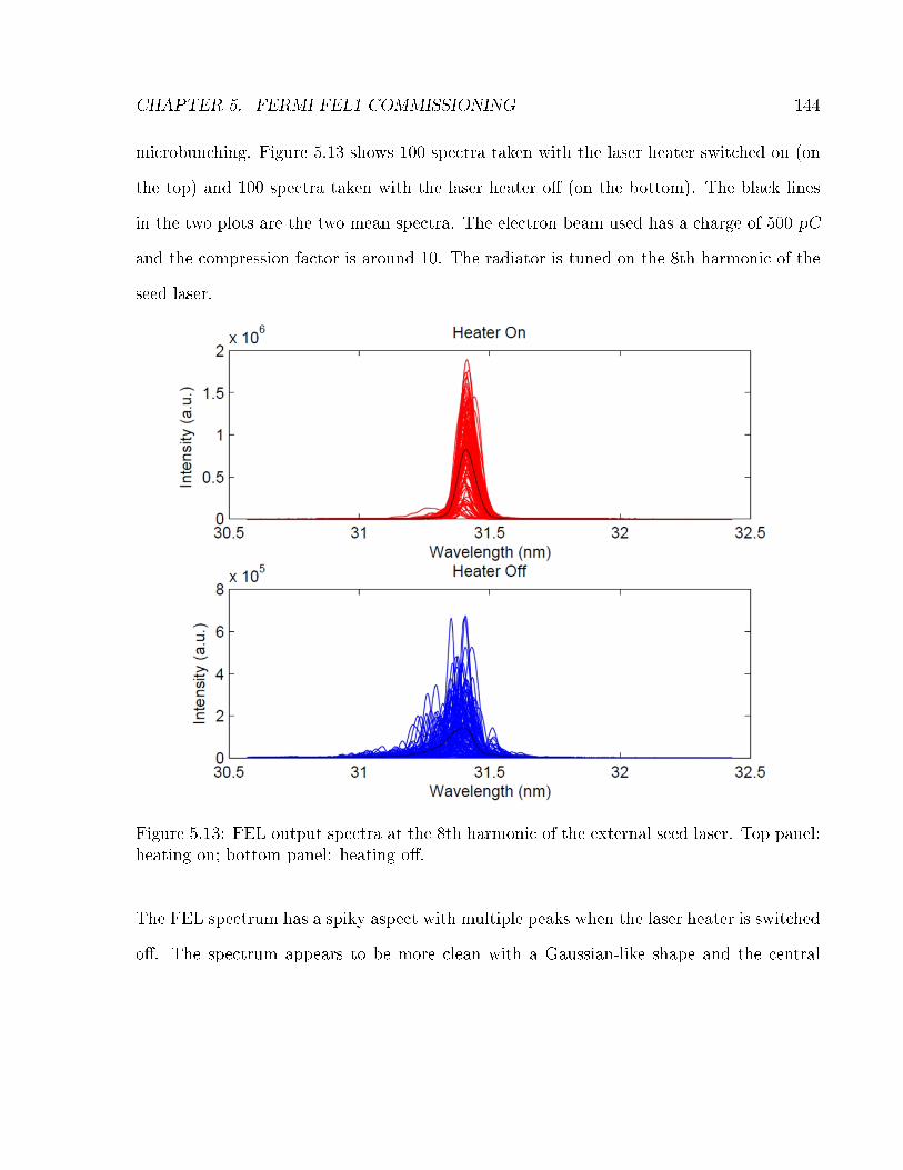
CHAPTER 5. FERMI FEL1 COMMISSIONING 144
microbunching. Figure 5.13 shows 100 spectra taken with the laser heater switched on (on
the top) and 100 spectra taken with the laser heater o� (on the bottom). The black lines
in the two plots are the two mean spectra. The electron beam used has a charge of 500 pC
and the compression factor is around 10. The radiator is tuned on the 8th harmonic of the
seed laser.
Figure 5.13: FEL output spectra at the 8th harmonic of the external seed laser. Top panel:heating on; bottom panel: heating o�.
The FEL spectrum has a spiky aspect with multiple peaks when the laser heater is switched
o�. The spectrum appears to be more clean with a Gaussian-like shape and the central

CHAPTER 5. FERMI FEL1 COMMISSIONING 145
wavelength is more stable when the laser heater is switched on. The mean bandwidth
varies, in this set of data, from 0.052 nm to 0.029 nm, while the stability of the central
frequency goes from 0.055 nm to 0.015 nm when the laser heater is switched on. The e�ect
of the laser heater on the FEL spectrum is evident also at higher harmonics. Figure 5.14
shows 60 spectra taken with the laser heater switched on (on the top) and 60 spectra taken
with the laser heater o� (on the bottom). The black lines in the two plot are the two mean
spectrum. The electron beam used has a charge of 500 pC and the compression factor is
around 10. The radiator is tuned on the tenth harmonic of the seed laser.
Figure 5.14: FEL output spectra at the 10th harmonic of the external seed laser. Top panel:heating on; bottom panel: heating o�.
In this case the mean bandwidth varies from 0.063 nm to 0.015 nm while the stability of
the central frequency goes from 0.035 nm to 0.015 nm when the laser heater is switched

CHAPTER 5. FERMI FEL1 COMMISSIONING 146
on. The transverse RMS dimension of the laser pulse in the laser heater undulator used is
around 130 µm for these measurements.
5.5 Extremely high harmonics
It is possible to tune the radiators of FEL1 with the resonance to shorter wavelengths,
beyond the nominal interval of operation. As expected a pulse energy decreasing with the
harmonic number is obtained, but the radiation spot on the diagnostic CCD can be detected
at surprisingly high orders, as shown in section 5.15, up to the twenty-ninth harmonic (h29)
corresponding to a wavelength of about 9 nm.
Figure 5.15: Spot of the FEL mode at higher harmonic orders.

CHAPTER 5. FERMI FEL1 COMMISSIONING 147
In �gure 5.16 the spectrum for twenty-sixth harmonic is shown. The spectrum is acquired
by integrating for 5 seconds, corresponding to a sequence of �fty laser shots.
Figure 5.16: Spectrum of FEL1 tuned at 10 nm.
No signal was observed at harmonics higher than the twenty-ninth with the single stage
cascade FEL1 �gure 5.15. However the undulator of FEL1 may be con�gured as a double
stage cascade following, in the radiator, a layout similar to those used in [172, 173] and
represented in �gure 5.17. In this con�guration the �rst undulators of the radiator are
tuned to one harmonic of the seed, as in the nominal con�guration of FEL1, and the last
undulators are tuned to one harmonic of the previous ones. The FEL growth, in the last
stage, starts directly from one harmonic of the bunching produced in the previous radiator.
In the case shown in �gure 5.17 we tuned the �rst four undulators of the radiator to the
thirteenth harmonic of the seed and the last two to the second harmonic of the previous
one (twenty-sixth harmonic of the seed).

CHAPTER 5. FERMI FEL1 COMMISSIONING 148
Figure 5.17: FEL1 in double stage cascade con�guration. In this con�guration the �rstundulators of the radiator are tuned to one harmonic of the seed, as in the nominal con�gu-ration of FEL1, and the last undulators are tuned to one harmonic of the previous ones. Inthe example shown the �rst undulators of the radiator are tuned to the thirteenth harmonicof the seed and the last undulators are tuned to the second harmonic of the previous ones.Courtesy of L. Giannessi.
The stronger ampli�cation of a lower order harmonic in the �rst undulator part, leads to a
stronger bunching and emission in the second part. This con�guration tuned to reach the
same �nal wavelength of 10 nm, was tested in the same e-beam condition of those used to
measure the spectrum in �gure 5.16. The relevant spectrum is shown in �gure 5.18.
Figure 5.18: Spectrum of FEL1 con�gured as a double stage cascade as shown in �gure5.17.
Despite the fact that the spectrometer was not calibrated in energy, the acquisition in the
two cases of the �gures 5.16 and 5.18, is done in the same conditions. We can therefore
compare the counts on the vertical scale in the two cases, and observe that the intensity
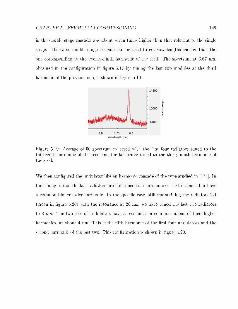
CHAPTER 5. FERMI FEL1 COMMISSIONING 149
in the double stage cascade was about seven times higher than that relevant to the single
stage. The same double stage cascade can be used to get wavelengths shorter than the
one corresponding to the twenty-ninth harmonic of the seed. The spectrum at 6.67 nm,
obtained in the con�guration in �gure 5.17 by tuning the last two modules at the third
harmonic of the previous one, is shown in �gure 5.19.
Figure 5.19: Average of 50 spectrum collected with the �rst four radiators tuned to thethirteenth harmonic of the seed and the last three tuned to the thirty-ninth harmonic ofthe seed.
We then con�gured the undulator like an harmonic cascade of the type studied in [174]. In
this con�guration the last radiators are not tuned to a harmonic of the �rst ones, but have
a common higher order harmonic. In the speci�c case, still maintaining the radiators 1-4
(green in �gure 5.20) with the resonance at 20 nm, we have tuned the last two radiators
to 8 nm. The two sets of undulators have a resonance in common at one of their higher
harmonics, at about 4 nm. This is the �fth harmonic of the �rst four undulators and the
second harmonic of the last two. This con�guration is shown in �gure 5.20.

CHAPTER 5. FERMI FEL1 COMMISSIONING 150
Figure 5.20: FEL1 in a harmonic double stage cascade con�guration. The �rst four undula-tors are tuned at 20 nm and the last two undulator are tuned to 8 nm. The �fth harmonicof the �rst stage is tuned to the second harmonic of the last two undulators. Courtesy ofL. Giannessi.
The spectrum obtained in this con�guration is shown in �gure 5.21.
Figure 5.21: Spectrum of FEL1 in a harmonic double stage cascade con�guration.
The upper image represents the spectrometer CCD raw data. The vertical axis is not
dispersed in frequency and provides information about the vertical intensity distribution at
the spectrometer. The double lobe structure of the y trace is typical of the even harmonic
emitted o�-axis in a circularly polarized undulator.
Chapter 6
Self-seeding
In the previous chapter we have seen that seeded FELs based on the HGHG scheme can
provide powerful, nearly Fourier transform limited, radiation pulses from the VUV down to
the soft X-ray regime. The highest harmonic of the seed laser wavelength, 260 nm, obtained
at FERMI is the 65th, i.e. 4 nm. Pushing the harmonic number further to reach hard X-
ray regime seems, at the moment, di�cult. A powerful and reliable seed source at short
wavelengths ≈10 nm, is not available at the moment. For this reason other mechanisms,
alternative to external seeding, to obtain coherent pulses in the hard X-ray region have to
be found. Due to the absence of a short wavelength seed laser it seems reasonable to start
from SASE. In this chapter we describe the so-called self-seeding technique and we present
the �rst hard X-ray self -seeding experiment done at LCLS with relative simulations.
151

CHAPTER 6. SELF-SEEDING 152
6.1 SELF-SEEDING
The SASE con�guration works by amplifying shot noise and for this reason it is considered
the natural option to produce short and powerful radiation pulses in the soft and X-ray re-
gion where laser source for external seeding are not available. LCLS, SACLA and FLASH,
the three SASE FELs working in the VUV and X-ray regime, have demonstrated at least
ten orders of magnitude of increase in brightness with respect to the third generation of light
sources delivering sub-picosecond pulses. The operations of these machines have con�rmed
the poor longitudinal coherence and intrinsic wide bandwidth of SASE FELs. A straight-
forward scheme, called self-seeding, to improve the longitudinal coherence of SASE has
been proposed in [76]. Self-seeding consists of two long undulators separated by an electron
beam chicane in which a monochromator is installed. The �rst undulator works in SASE
con�guration without an external seeding. The radiation produced in the �rst undulator is
puri�ed by the monochromator and then used as coherent seed for the second undulator.
The monochromator can produce a delay of the light with respect to the straight line and
the electron path in the chicane has to be adjusted to provide synchronization between the
two beams in the second undulator. The beam coming from the �rst SASE undulator has a
density modulation with a broad spectrum content resulting from the shot noise ampli�ca-
tion within the FEL bandwidth in the �rst undulator. The presence of energy and density
modulation in the FEL bandwidth can spoil the longitudinal coherence and spectral quality
of the light ampli�ed in the second undulator. The R56 of the chicane and the energy spread
of the electron beam washes out the microbunching produced in the �rst undulator.
The �rst article about self-seeding presented an application of the technique at 6 nm wave-
length and was devoted to soft X-ray regime. In this spectral range, the type of monochro-

CHAPTER 6. SELF-SEEDING 153
mator used to purify SASE can be based on a grating. The time delay of the light with
respect to the electrons depends on the number of mirrors and on the geometry used and is
in the range 800 fs-5 ps. A conventional 4-crystals monochromator can be used to extend
the self-seeding technique to the hard X-ray regime but the time delay of the light cannot
be shorter than 10 ps. This delay requires, in the single bunch con�guration, a long chicane
in which the light produced by one bunch in the �rst monochromator is ampli�ed by the
same bunch in the second undulator. Such a chicane can degrade the electron beam quality
through incoherent and coherent synchrotron radiation. Recently a straightforward tech-
nique to achieve self-seeding in the hard X-ray regime with a single bunch has been proposed
[175] and successfully demonstrated in LCLS [76]. This technique uses a single crystal in
forward Bragg di�raction (FBD) [176] geometry on which the SASE pulse produced in the
�rst undulator impinges. The layout of this scheme is shown in �gure 6.1.
Figure 6.1: Scheme of the hard X-ray self-seeding based on the crystal monochromator.The �rst undulator is separated from the second one by a chicane for the electron beam. Acrystal, placed in Bragg geometry in the chicane, intercepts the SASE (pale magenta beam)radiation produced in the �rst undulator. Part of the radiation component satisfying theBragg condition is re�ected (blue beam). The rest of the radiation satisfying the Braggradiation, that is not re�ected, is transmitted with a delay with respect to the SASE com-ponents that not satis�es the Bragg condition. The position of the re�ected radiation onthe screen, shown in the picture, identi�es the angle θ.

CHAPTER 6. SELF-SEEDING 154
The angle between the crystal and the SASE propagation direction is chosen to satisfy the
Bragg condition for one component of the SASE spectrum. This component experiences
multiple scattering in the crystal and it is partially re�ected. The spectrum of the re�ectance
exhibits a narrow line width and the transmission spectrum exhibits an absorption reso-
nance. The crystal acts like a band pass �lter. The Bragg angle satis�es the condition
[177]:
2dssinθ = λr (6.1)
where ds is the spacing between crystallographic planes, θ is the angle between the crystal
and impinging radiation and λr is the wavelength that experiences Bragg re�ection. The
forward scattered radiation acquires a phase shift required by causality and that can be
calculated by the Kramer Kronig [178-180] relation from the transmittance spectrum. This
shift produces a delay in the time domain. The rest of the SASE spectrum that does not
satisfy the Bragg condition is transmitted without delay and is followed by a monochromatic
wake formed by the component identi�ed by the Bragg condition. The time duration of the
wake is inversely proportional to the bandwidth of the absorption line. The wake exhibits
multiple peaks of decreasing intensity for increasing time delay. The delay at which the
maxima are located and the duration of bumps depends on the crystal structure. The
properties and underlying physics of FBD relevant to this application are discussed in detail
in [176]. Here, we only highlight that the time dependence t of the radiation envelope of
FBD, G00(t), which represents the crystal response to a very short incident pulse, can be

CHAPTER 6. SELF-SEEDING 155
parameterized with the characteristic timescale T0:
|G00(t)|2 ∝
1
T0
J1
(√tT0
)√
tT0
2
(6.2)
with T0 = Λ2sinθ2π2cd
were Λ is the extinction depth [177] and d is the crystal thickness. The
delay of the �rst maximum is of the order of 10-20 fs and then a very gentle chicane
is enough to delay the electron beam to establish the seed ampli�cation in the second
undulator. This chicane provides the room for the crystal and is useful to wash out the
microbunching produced in the SASE radiator. For the single crystal wake monochromator,
the ratio between the peak power in the �rst bump and the SASE power can be related to
the pulse duration of the SASE pulse, the SASE coherence length and the location of the
�rst maximum:
Pmaxseed
PSASE=LSASELcoherence
cτ 21
(6.3)
This scheme has been successfully demonstrated in LCLS in the �rst self-seeding experiment.
6.2 LCLS experiment: results
Here, we describe some initial results from the HXRSS experiment at LCLS. The LCLS
nominally operates at 150�250 pC of charge in a single electron bunch at a repetition rate

CHAPTER 6. SELF-SEEDING 156
of 120 Hz. However, the machine can also be run in a low-charge mode [140] where only
20�40 pC of charge is used to generate a much shorter pulse length of 5�10 fs, but with pro-
portionally fewer photons (0.2 ·1012 photons per pulse at 8 keV ). This short pulse provides
good overlap with the short seed wake pulse produced by the diamond monochromator and
is used for the self-seeded mode of operation. As described above, the low-charge SASE
mode of operation produces very limited longitudinal coherence and a broad, noisy photon
spectrum with a relative spread of 0.25% full-width at half-maximum (FWHM; 20 eV ). The
self-seeded mode is designed to dramatically improve the bandwidth and coherence. The
self-seeded mode is established by inserting the diamond crystal in the SASE X-ray beam
path to generate the monochromatic seed pulse and using the chicane to delay the electrons
by 20 fs to overlap the seed. The Bragg angle of the diamond crystal is chosen for the de-
sired seeding wavelength. By adjusting the electron energy, the SASE spectrum produced
by the �rst undulator stage should fully cover this seeding wavelength. An angle θ=56.538
(see �gure 6.1) corresponds to the Bragg re�ection condition from the (004) atomic planes
of diamond for 8.3 keV photons near the K-edge of nickel. The energy of the electron beam
is adjusted to 13.71 GeV to be resonant with the seed. The extinction depth for the 004
re�ection of our crystal is Λ = 22.6µm, so that we obtain from equation 6.2 ts = 19 fs for
the location of the �rst maximum of the monochromatic �eld with respect to the incident
pulse. The crystal time response ∝ |G00|2 equation 6.2 is plotted in �gure 6.2.

CHAPTER 6. SELF-SEEDING 157
0 20 40 60 80 1000
20
40
60
80
100
120
Time Delay (fs)
|G00
(t)|
2
Crystal Time Response
Figure 6.2: Time responses |G00|2 to excitation with a short X-ray pulse in FBD. Re�ectionfrom the atomic planes (004) of diamond. Results for diamond crystals with thickness d=0.1mm.
The un�ltered SASE pulse is superimposed on the monochromatic wake in the �rst 10 fs of
the time scale in �gure 6.2. The �rst monochromatic bump, useful for self-seeding, has a
time duration of ≈15-20 fs. The transverse overlap between the seed and the electron beam
can be optimized by slightly varying the electron position and angle using the undulator
girder position remote control at the beginning of the second undulator stage.
The peak power available in the monochromatic seed can be estimated by equation 6.3.
The coherence length is around 60 nm and the pulse length is around 5 fs and, with these
parameters the maximum power of the �rst bump is 0.25% of the SASE power. We calculate
the evolution of the FEL pulse along the SASE undulator using the equation 2.45 for the
high-gain regime replacing LG with L1d (equation 2.50). From the previous considerations
and calculations we �nd that the peak seed power at the end of the �fteenth undulator is:

CHAPTER 6. SELF-SEEDING 158
Pseed ≈0.0025·
9exp(
14 · LULG
) · P (0) ≈0.0025·
9exp(12) · Pnoise ≈ 35 · Pnoise (6.4)
where the number of the undulators has been reduced, in equation 6.2, by one to take into
account the lethargy and a mean gain length of 4 m has been considered [140]. The shot
noise equivalent power is indicated as Pnoise (2.64). Therefore the seed power generated
in the �rst �fteen undulators easily overcomes the shot noise, ensuring the seed power
requirements for the self-seeding experiments.
Although up to 15 undulator segments upstream of the seeding section (U1�U15) can be
used to generate SASE, which is then `�ltered' by the diamond for seeding, too much SASE
radiation actually induces a large growth of the electron energy spread, which then inhibits
the gain process for the seeded FEL in the second stage. There is therefore a trade-o�
between seeding power and seeded FEL gain. Experimentally, we �nd that using only 13
SASE undulator segments (U3�U15) seems to produce the most seeded FEL power at the
end of the LCLS undulator line. The typical SASE pulse energy produced by 13 undulator
segments is 10 µJ with 40 pC of bunch charge. Another 13 undulator segments (U17�U29)
downstream of the seeding section amplify the seeded signal. Figure 6.3 shows the gas
detector signal (X-ray pulse calorimeter), located well after U29, when the chicane was
operated in the self-seeding mode. The left side of this time plot was taken when the
diamond crystal was retracted from the X-ray beam path, showing a 19µJ mean SASE
background, while the right side was taken when the diamond crystal was inserted, showing
a 53 µJ mean seeded FEL signal, including the 19 µJ SASE background. Because the
seed power is generated from the random SASE process and �uctuates close to 100% before
saturation and when a single longitudinal mode is selected, the output FEL energy �uctuates

CHAPTER 6. SELF-SEEDING 159
nearly as much for this linear ampli�er. In addition, electron energy jitter of 0.05% r.m.s
also contributes signi�cantly to the FEL intensity �uctuation. Peak seeded intensities in
excess of 200 µJ have been observed at a bunch charge of 40, but, to date, the variations
in shot-to-shot intensity remain larger than 50%.
Figure 6.3: Each data point is an FEL X-ray pulse total energy measurement made usingthe gas detector and plotted against the vertical position of the diamond crystal (y). TheX-ray beam falls o� the crystal edge at y=-2 mm, showing the SASE background at y<-2mm with a mean pulse energy of 19 µJ (solid blue line). The seeded signal (plus the SASEbackground) is shown at y>-2 mm with a mean energy of 53 µJ (dashed blue line) andpeaks at 150 µJ. This does not show the best seeded performance but does re�ect the largepower �uctuations observed. The chicane is switched on here, which greatly reduces theSASE power from that of normal SASE operation. Taken from [77].
Figure 6.4a shows the single-shot SASE and self-seeded spectra recorded on a Si (333) bent
crystal spectrometer [76] with an estimated resolution of 0.1 eV. The zero point in the
horizontal axis refers to the mean photon-energy of 8331.5 eV (0.14881 nm). The SASE
spectrum is produced with all 28 undulators, that is, with the chicane o� and diamond
CHAPTER 6. SELF-SEEDING 160
retracted. In this case, the optimized SASE pulse energy is 300 µJ with 20 eV FWHM
bandwidth. The seeded signal reaches 240 µJ, and shows a single spectral spike of 0.4
eV (FWHM). The relative FWHM bandwidth is 5 · 10−5 at 8.3 keV, which corresponds to
a Fourier-transform-limited X-ray pulse of 5 fs (FWHM). Figure 6.4b shows the average
SASE spectra for 20,000 shots taken on a Si (111) spectrometer, with a wider range to
accommodate the electron energy jitter (on the order of 8�10 eV RMS). The FWHM of
the average SASE bandwidth is 27 eV without energy jitter correction (as shown) and
becomes 20 eV by correcting the electron energy on a shot-by-shot basis. It also shows the
average seeded spectra over 200 shots taken on an Si(333) spectrometer under good seeding
conditions. The FWHM bandwidth of the average seeded spectrum is 1 eV. The broadened
average bandwidth comes from shot-to-shot spectral variations due to electron energy jitter
and other factors. The seeded FEL has a Gaussian spatial mode with excellent transverse
coherence. The simulations, as we will see in the next section, indicate that the seeded
FEL spectra are quite sensitive to the detailed longitudinal phase space distribution of the
electron beam and suggest further improvements in the seeding performance.

CHAPTER 6. SELF-SEEDING 161
Figure 6.4: Single-shot (a) and averaged (b) X-ray spectrum in SASE mode (red) and self-seeded mode (blue). The FWHM single-shot seeded bandwidth is 0.4 eV, whereas the SASEFWHM bandwidth is 20 eV. Vertical scales have the same arbitrary units in both a and b.The chicane is turned o� for the SASE measurements, but necessarily switched on for theself-seeded mode. Taken from [77].
The chicane strength has also been varied to scan the electron delay so as to trace out the
monochromatic wake pulse generated by the diamond crystal. Because the gas detector

CHAPTER 6. SELF-SEEDING 162
contains signi�cant SASE background, we use the spectrometer signal and zoom into the
narrow-bandwidth seeded spectra for this study. Figure 6.5 shows the seeded FEL intensity
as a function of the chicane delay, re�ecting the time dependence of the FBD intensity
envelope, in reasonable agreement with FBD theory predictions. The peak seeded signal is
reached at a chicane delay of 19 fs, in agreement with the value calculated by equation 6.2.
The relatively large error bars for the data (standard deviation) indicate the �uctuating
nature of the seeded power, as discussed above.
Figure 6.5: Seeded FEL intensity as a function of chicane delay, measured using the intensityof just the narrow seeded line on the X-ray spectrometer. The points are the spectrometersignal and the solid curve is the convolution of the di�raction theory prediction of equation(1) with the X-ray pulse duration. Crystal thickness and X-ray pulse duration are taken tobe �tting parameters. The best �t is obtained when d=104 µm with a �at-top X-ray pro�leof 5.5 fs. Taken from [77].
Finally, in �gure 6.6, we show the measurements of the gain length in the SASE undulator
and in the seeded undulator.

CHAPTER 6. SELF-SEEDING 163
Figure 6.6: Gain length measurements in SASE undulator and seeded undulator. Courtesyof D. Ratner.
6.3 LCLS self-seeding experiment: simulations and re-
sults analysis
In this section, we present detailed simulations that can help to understand the system
performance and optimization. The results of the self-seeding experiments are determined
by the electron beam properties and by the energy and peak power of the seed ampli�ed
in the second undulator. Both are not completely known. The knowledge of the current
beam pro�le and other beam slice properties is extremely di�cult to obtain for the 20
pC and the 40 pC mode as the bunches have a duration of 10 fs. The current beam
pro�le can be measured, with limited resolution, through a modi�cation of the zero phase
CHAPTER 6. SELF-SEEDING 164
technique described by [181]. The process of seed generation in the crystal has been studied
in [175, 176]. Both these two studies predict, starting from two di�erent approaches, a
similar level of power. A measurement of the seed characteristics, even if not possible
with the current experimental setup, seems to be very important for the understanding of
experiments results. The seeding e�ciency can be reduced by a misalignment or an angle
between the electron beam and the seed. Knowledge of the global seeding e�ciency and of
the interplay between electron beam proprieties and the obtained FEL power and bandwidth
it is important for planning regular users' utilization in LCLS and in the development of
other machines [182]. In the present work, we try to derive as much as possible about the
evolution of the FEL pulse in the two undulators from the experimental data using basic
physics concepts. We can guess the fundamental characteristics of the electron bunch and
the seed power from the experimentally derived model. Then we compare the result of these
studies with start to end simulations starting from beam generated in the photoinjector by
IMPACT-T [183] and tracked in the linac with elegant [165]. The simulations of the FEL
process in the undulator are done with the code Genesis 1.3 [160]. Some beam parameters
can be checked with measurements of current beam pro�le. Recently a technique based
on a high energy resolution spectrometer has been implemented in LCLS to measure the
longitudinal current pro�le of the 20 pC and 40 pC electron bunch. The third linac section
operates at 0 degree RF crossing phase with no net acceleration to provide a linear energy
chirp during the measurements of the beam pro�le. It has been shown that it is possible to
have a one to one relationship between the longitudinal coordinate after the second bunch
compressor and the energy coordinate after the third linac if a third chicane is located
between the second bunch compressor and the third linac when the R56 of this third chicane

CHAPTER 6. SELF-SEEDING 165
satis�es the following relation [181]:
1 + hR56 = 0 (6.5)
where h is the linear chirp that the beam acquires in the third linac section. When this
condition is satis�ed the relation between the longitudinal coordinate after the second bunch
compressor and the energy coordinate after the third linac is simply:
hZi = δi (6.6)
where Zi and δi are the longitudinal and the energy coordinate of the i particle with respect
to the centre of mass and to the mean energy respectively. The energy coordinate at the
end of the linac depends only on the longitudinal coordinate of the particle in the beam
after the bunch compressor. The beam is sent into a high resolution energy spectrometer
and the energy is converted in the horizontal coordinate. The horizontal coordinate of
the spectrometer screen corresponds to the longitudinal coordinate of the beam while the
vertical coordinate of the screen corresponds to the vertical coordinate of the beam (see the
top of the �gure 6.8). Projection of the image along the horizontal coordinate yields the
beam current pro�le. At this point the x pro�le recorded on the spectrometer screen is a
magni�ed image of the beam longitudinal pro�le after the second compressor. The R56 of the
second chicane is increased by a term that satis�es the relation (6.5) in the implementation
of the method in LCLS. This is equivalent to adding a third chicane and it does not require
hardware modi�cations. The pro�le of the beam is recorded as a function of the phase of
the second linac. Figure 6.7 shows the bunch current pro�le measured with the technique

CHAPTER 6. SELF-SEEDING 166
described above for two consecutive electron beam shots. The linac setting during these
measurements is the same as that used during the FEL self-seeding experiments. We can
see that the current pro�le changes signi�cantly from shot to shot.
Figure 6.7: Bunch pro�le of two consecutive shots. The head of the bunch is at negativetime.
An energy chirp is still present on the beam at the linac end and therefore the bunch can be
compressed by the negative R56 of the transfer line leading to the undulator line. For this
reason, the beam pro�le in the undulator is not exactly the one that it is measured by the
described method. A correspondence can be established between the measured pro�le and
the actual one in the undulator. In �gure 6.8 we show the images on the spectrometer screen
(on the top) and the corresponding current in the undulator obtained from linac simulations
(on the bottom) for three di�erent compression settings. The horizontal coordinate of the
screen corresponds to the beam energy and to the longitudinal coordinate of the beam
through the relation 6.5 while the vertical coordinate of the screen corresponds to the
vertical coordinate of the beam. We can see that the shape of the electron beam current
seen in the screen is preserved.

CHAPTER 6. SELF-SEEDING 167
Figure 6.8: On the top: Three images of the electron beam on the spectrometer screen forthree di�erent compressions. On the bottom: The corresponding current in the undula-tor obtained from linac simulations for the same three compression settings used for themeasurements shown above (courtesy of J. Wu).
A large number of pulses are characterized by a double horns distribution. We use such
a beam produced in injector-linac simulations as starting point for the FEL simulations
with Genesis 1.3. The current pro�le of the beam used and other slice parameters used in
the start to end simulations are shown in �gure 6.9. Figure 6.9a shows the beam current
pro�le. Figure 6.9b shows variation of the mean energy of each slice along the beam, 〈γ〉,
with respect to the mean beam energy γ0 along the beam. Figure 6.9c reproduces the
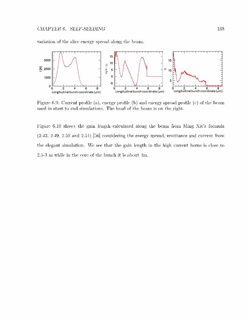
CHAPTER 6. SELF-SEEDING 168
variation of the slice energy spread along the beam.
Figure 6.9: Current pro�le (a), energy pro�le (b) and energy spread pro�le (c) of the beamused in start to end simulations. The head of the beam is on the right.
Figure 6.10 shows the gain length calculated along the beam from Ming Xie's formula
(2.43, 2.49, 2.50 and 2.51) [56] considering the energy spread, emittance and current from
the elegant simulation. We see that the gain length in the high current horns is close to
2.5-3 m while in the core of the bunch it is about 4m.
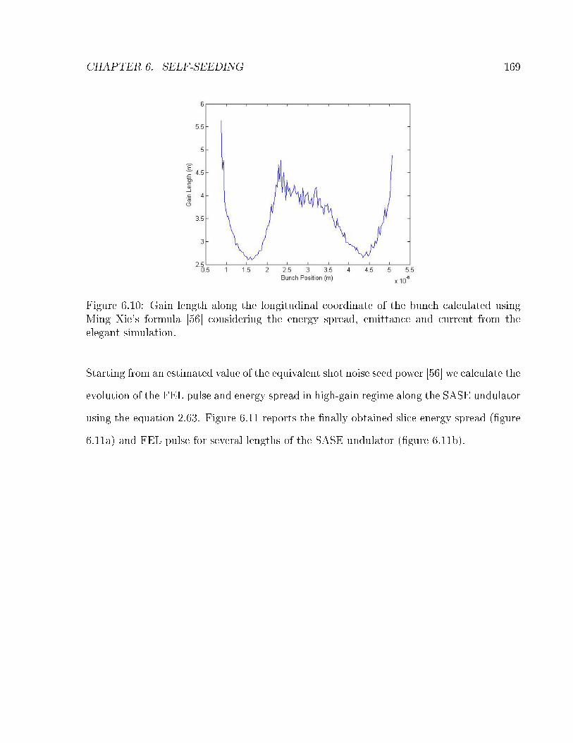
CHAPTER 6. SELF-SEEDING 169
Figure 6.10: Gain length along the longitudinal coordinate of the bunch calculated usingMing Xie's formula [56] considering the energy spread, emittance and current from theelegant simulation.
Starting from an estimated value of the equivalent shot noise seed power [56] we calculate the
evolution of the FEL pulse and energy spread in high-gain regime along the SASE undulator
using the equation 2.63. Figure 6.11 reports the �nally obtained slice energy spread (�gure
6.11a) and FEL pulse for several lengths of the SASE undulator (�gure 6.11b).

CHAPTER 6. SELF-SEEDING 170
Figure 6.11: a: Energy spread. b: FEL power evolution along the SASE undulator. Cyancurve refers to eleven undulators, green is for twelve undulators and magenta is for thirteenundulators.
The variation of the gain length along the bunch pro�le a�ects the evolution of the energy
spread and of the FEL power along the undulator. Twelve undulators are equivalent, in
the horns and in the core of the bunch, respectively, to about 15 and 10 gain lengths. The
energy spread is increased in a signi�cant way only in the horns. The horns produce a
great part of the total FEL power too. Then we calculate the value of seeded FEL pulse
mean power as function of the number of the SASE undulator sections. The power shown
in �gure 6.11b) is multiplied for several values of monochromatic e�ciency and used to
evaluate the evolution of the seeded power according to the equations 2.56 and 2.63. The
seed is considered as �at with a constant power completely covering the electron beam. For
each number of SASE undulators used, we have several values of the power obtained at the
end of the second undulator according to the considered e�ciency. The results are shown
in �gure 6.12.

CHAPTER 6. SELF-SEEDING 171
Figure 6.12: Seeded main power versus the number of SASE sections for several monochro-matic e�ciencies.
This analytical model predicts that the maximum output energy is produced using only
twelve undulator in the SASE section.
Now we performed FEL simulations of the SASE undulator with the code Genesis 1.3 using
the beam illustrated in �gure 6.9. Figure 6.13a shows the growth of the pulse energy along
the SASE undulator averaged over thirteen simulations performed with di�erent seeds for
the shot noise [56]. The gain length is ≈3.5 m. The pulse energy after thirteen undulators is
7±3 µJ. The typical temporal shape of the FEL pulse produced in thirteen SASE undulators
is shown in �gure 6.13b. The SASE pulses have a shape characterized by two narrow peaks.
The energy spread pro�le after twelve, thirteen and �fteen SASE undulators is shown in
�gure 6.13c.

CHAPTER 6. SELF-SEEDING 172
Figure 6.13: a: Growth of the pulse energy along the SASE undulators chain averaged onthirty simulations performed with di�erent seed for the shot noise. The gain length is ≈3.5m. The pulse energy after thirteen undulators is 7 ± 3 µJ . b: Typical temporal shapeof the FEL pulse produced in thirteen SASE undulators. The SASE pulses have a shapecharacterized by two high and narrow peaks. c: Energy spread pro�le after twelve, thirteenand �fteen SASE undulators. The head of the beam is on the right.
We see that the evolution of the SASE pulse, and consequently of the energy spread, in the
head of the bunch is reduced with respect to the analytical calculation. This is an e�ect of
the energy pro�le (�gure 6.9b), of the wake �elds and of the linear taper used to compensate
wake �elds and synchrotron radiation. For this reason a part of the beam, located near the
head of the bunch is still not spoiled by energy spread after thirteen undulators (see �gure
6.13c) and the optimum number of SASE sections is increased by one with respect to that
calculated analytically.
Almost all of the self-seeding experiments have been done using 13 undulators in the SASE
stage and this partially con�rms the simulations. Experimentally, a gain length of 3.9 m
meter has been observed in the SASE undulator, and the measured energy at the crystal is
≈10 µJ consistent with the simulations.
SASE is an exponential ampli�cation of the shot noise. Using the knowledge of the noise
power, we can estimate the temporal duration of the gain medium, the portion of the

CHAPTER 6. SELF-SEEDING 173
electron beam, that produces 10 µJ in thirteen sections with the measured gain length.
Using the gain length calculated for the horn, and considering one gain length for lethargy
we obtain that a shot noise energy of about 0.01 nJ is ampli�ed to produce ≈10 µJ after
thirteen sections. The shot noise power is in the range of 2-5 kW for the current level of
the 40 LCLS beam. Considering a shot noise power in this range, we obtain that almost
only a portion of the beam as long as ≈3 fs (1µm) is lasing. This estimate is also consistent
with the start to end simulations which indicate that almost only the horns of the beam
are contributing to produce the emitted radiation. The temporal pro�le of the FEL pulse
at the end of the SASE undulator is dominated by two very narrow structures, as shown in
�gure 6.12b, con�rming the supposed scenario.
Now we performed simulations of the seeded undulator with the code Genesis 1.3. We show
the results of these simulations in the �gure 6.14. The �gure 6.14a reports the growth of the
pulse energy along the seeded undulator. The seed used in this simulation has a peak power
of 5 MW in agreement whith simulations of the SASE undulator and with the expected
monochromator e�ciency.
The gain length obtained by simulation is 5 m in good agreement with the experimental
results (see �gure 6.6a). The pulse energy after thirteen seeded undulators is about 250 µJ.
The maximum pulse energy obtained in the hard X-ray self-seeding experiment at the end
of the seeded undulator, including 13 sections (U17-U29), is in the range of 200-250 µJ. The
temporal shape of the FEL pulse at the end of the thirteen undulator section is shown in
�gure 6.14b. The pulse has a duration (FWHM) of ≈10 fs. Figure 6.14c reproduces the
spectrum of the seeded pulse obtained in this simulations. The zero point on the horizontal
axis refers to the mean energy of 8331.5 eV (0.14881 nm). The FWHM relative bandwidth
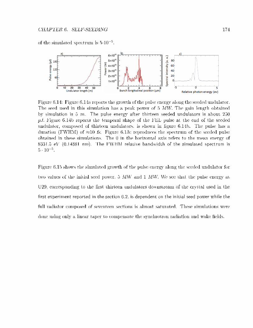
CHAPTER 6. SELF-SEEDING 174
of the simulated spectrum is 5·10−5.
Figure 6.14: Figure 6.14a reports the growth of the pulse energy along the seeded undulator.The seed used in this simulation has a peak power of 5 MW. The gain length obtainedby simulation is 5 m. The pulse energy after thirteen seeded undulators is about 250µJ. Figure 6.14b reports the temporal shape of the FEL pulse at the end of the seededundulator, composed of thirteen undulators, is shown in �gure 6.14b. The pulse has aduration (FWHM) of ≈10 fs. Figure 6.13c reproduces the spectrum of the seeded pulseobtained in these simulations. The 0 in the horizontal axis refers to the mean energy of8331.5 eV (0.14881 nm). The FWHM relative bandwidth of the simulated spectrum is5 · 10−5.
Figure 6.15 shows the simulated growth of the pulse energy along the seeded undulator for
two values of the initial seed power, 5 MW and 1 MW. We see that the pulse energy at
U29, corresponding to the �rst thirteen undulators downstream of the crystal used in the
�rst experiment reported in the section 6.2, is dependent on the initial seed power while the
full radiator composed of seventeen sections is almost saturated. These simulations were
done using only a linear taper to compensate the synchrotron radiation and wake �elds.

CHAPTER 6. SELF-SEEDING 175
Figure 6.15: Simulated growth of the pulse energy along the seeded undulator for two valuesof the initial seed power, 5MW and 1MW. U29 corresponds to the �rst thirteen undulatorsdownstream of the crystal used in the �rst experiment reported in the section 6.2.
The �uctuations of the seed power, inherited from the stochastic nature of SASE, complicate
the utilization of the quadratic taper to extract more energy above the saturation level.
Indeed di�erent values of the seed required di�erent locations at which the quadratic taper
should starts. High power seeds require to start the quadratic taper closer to the crystal
compared to the low power seeds. The �uctuations of the �nal energy related to the seed
energy are larger when the taper is optimized for the maximum seed power available and
saturation is not observed at U33. The RMS energy jitter at the end of the linac is 0.05%
and 30% of the pulses is not seeded due to the energy �uctuation of the electron beam as the
bandwidth of the seed is of the order of ≈10−5 [176, 177] and this increases the pulse energy
�uctuations. For these two reasons pulse energy �uctuations of the order of 30%-50% are
usually observed even when 17 undulators are used after the crystal.
Now we try to derive the ampli�ed seed energy and the maximum seed power from the
available data. Considering the �nal maximum energy of 250µJ obtained in thirteen seeded

CHAPTER 6. SELF-SEEDING 176
undulators, the gain length of 5 m and one gain length for lethargy, we can state that the
ampli�ed maximum seed energy is 50 nJ. Supposing that the seed peak power is about 5
MW we obtain that the ampli�cation process happens on a part of the beam about 10 fs
long. This is in good agreement with the shape of the pulse from simulations. Now we try
to estimate the seeded FEL pulse length from spectral considerations. As stated before the
single-shot relative bandwidth for good high energy shots corresponds to a Fourier transform
limited pulse of 4-5 fs. The pulse can still be longer than 5 fs in the case that its Fourier
limited bandwidth is shorter than the measured one with the pulse bandwidth increased
by a chirp on the beam. In particular, the experimental seed bandwidth and the estimated
pulse length of 10 fs determines a time-bandwidth product that is about 2 times the Fourier
limited one and this corresponds quite well to the simulation results. The FEL seeded pulse
obtained by spectral consideration is still shorter than the electron beam but longer than
the SASE one. Then we can guess that the core of the beam emits a good part of the FEL
energy but the horns, or at least one horn, still dominates. The start to end simulations
con�rm this scenario (�gure 6.13b).
Not all the seeded pulse have a pure Gaussian mode like that in �gure 6.4. Some spec-
trum (see �gure 6.16) shows sidebands and multiple peaks and this pulse to pulse spectral
variation causes the spectral broadening seen in the average spectrum.

CHAPTER 6. SELF-SEEDING 177
Figure 6.16: Self-seeded single-shot measured spectrum. 13 SASE undulators + 13 seededundulators.40 pC beam. Courtesy of A. Lutman.
Some spectra obtained in simulation are shown in �gure 6.17. The spectrum shown on the
left is obtained in start to end simulation with the second undulator detuned with respect
to the value that produces the spectrum shown in �gure 6.17. The spectrum shown on the
right is obtained using in simulation a �at energy distribution and the current pro�le from
start to end simulation.
Figure 6.17: Self-seeded single-shot simulated spectrum. 13 SASE undulator + 13 seededundulator. 40 pC beam. start to end simulation on the left. The spectrum shown on theright is obtained using in simulation a �at energy distribution and the current pro�le fromstart to end simulation.
The electron beam energy and shape is changing from shot to shot and this explains the
energy and spectral shot to shot �uctuations observed in the experiment. In the measure-

CHAPTER 6. SELF-SEEDING 178
ments shown in �gure 6.16 and in the simulation in 6.17 only a linear taper is used to
compensate synchrotron radiation and wake �eld losses. We have presented studies on the
hard X-ray self-seeding experiments at LCLS. Experimental data and start to end simula-
tions show that in the SASE undulator, the radiation is produced mainly by the horns of
the beam while in the seeded undulator the core of the beam starts to emit radiation. The
gain lengths and the level of pulse energy measured experimentally at the end of the two
undulators (SASE and seeded undulator) are in agreement with the simulations. Simula-
tions suggest that 10 µJ SASE radiation produced in the SASE stage (U3�U15) generates
su�cient seed power (5 MW ) but degrades the electron beam energy spread. As a result,
the FEL signal grows slower in the seeded stage due to increased energy spread and pro-
duces 250 µJ FEL pulse energy after 13 undulator segments (U17�U29), without reaching
saturation. The simulations also indicate that the seeded FEL spectra are quite sensitive
to the detailed longitudinal phase space distribution of the electron beam and explain the
�uctuations of the shape of the single-shot spectra and the broadening of the averaged spec-
trum. Further studies have shown the impact of the jitter of the electron beam energy on
the energy stability of seeded pulse.
Chapter 7
SASE with tapered undulator and chirp
In this chapter we will describe a method to improve the longitudinal coherence of SASE
radiation based on a linear energy chirp and on undulator tapering [74, 75]. The FEL line
used to implement this method is composed of a single long undulator as in the SASE
FEL. In this case the undulator is strongly tapered. It has been shown that the e�ect
of a linear energy chirp on the FEL gain [74] is equivalent to that of a linear undulator
tapering. Then it is possible to compensate the FEL spectrum broadening, caused by the
undulator tapering, by means of a linear energy chirp. It is possible, in this way to produce
a single Gaussian spike with a spectrum close to Fourier transform limit. We present, in this
chapter, the results of the �rst experiment done to test this method. These experimental
studies have been done at the SPARC test facility. This method, as it is self-seeding, does
not use a seed laser and can be extended, as in the original proposal, down to the hard
X-ray regime.
179

CHAPTER 7. SASE WITH TAPERED UNDULATOR AND CHIRP 180
7.1 Compensation of linear chirp by undulator tapering
This scheme combines an electron beam energy chirp with a chosen undulator �eld taper,
i.e., a smooth variation of peak magnetic �eld along the beam propagation axis, implemented
in SASE con�guration without an external seed. The basic idea behind this scheme is that
a symmetry between the energy chirp and the undulator tapering exists [74] and can be
understood by considering the radiation �eld acting on some test electron emitted at a
retarded time from an electron behind. A radiating electron, in the presence of an energy
chirp on the electron beam, has a detuning due to an energy o�set, while it has the same
detuning, in a tapered undulator, because the undulator parameters were di�erent at the
retarded time. We will see that these two e�ects can compensate each other. In case of a
linear chirp on the electron beam, the mean ``local'' energy varies as:
γ(s) = γ(s0) + α(s− s0) (7.1)
where s is the longitudinal bunch coordinate, s0 represents the centre of the electron bunch
in its drifting reference frame and α quanti�es the degree of energy chirp. The energy
chirp serves to detune the beam's local resonant frequency. The resonant frequency varies
along the beam in the presence of a chirp and the central radiation produced in a SASE
con�guration follows the resonance frequency. The higher velocity of the light with respect
to that of the electrons produces a slip of the radiation. As the FEL radiation produced
upstream propagates forward in s, it falls out of the local gain bandwidth when it slips a
distance of the order of:

CHAPTER 7. SASE WITH TAPERED UNDULATOR AND CHIRP 181
δs ∼ργm0c
2
2α(7.2)
where ρ is the Pierce parameter introduced in section 2.4. This e�ect can be compensated,
however, by choosing the undulator taper to allow the continuous gain of a spike initiated
in the rear of the bunch as it moves forward in s with the appropriate velocity, as illustrated
in �gure 7.1. Analysis of this slippage is complicated by the modi�cation of the radiation
spike's velocity in the presence of gain; the peak of a spike in the exponential gain regime
moves at a velocity [39]:
βL ∼3βZβZ + 2
(7.3)

CHAPTER 7. SASE WITH TAPERED UNDULATOR AND CHIRP 182
Figure 7.1: Propagation of a �eld spike (blue) developing at the rear of a chirped e-beam(green) for (a) untapered case, and (b) tapered case as a function of z. Vertical axesindicate the resonant condition as a function of the relative position between the beam andradiation, δ is the �nal detuning in the untapered case. In (a) the slippage leads the spikeout of resonance, when the chirp is combined with an appropriate undulator taper (b), theresonance can be preserved. Taken from [75].
Approaching saturation, the radiation peak propagates at a higher velocity than βL, closer
or even higher than unity, because of the pulse shortening associated with the electron
synchrotron oscillation [184]. Above saturation, the front of the pulse moves forward at
c. The chirp-taper combination discussed above also a�ects the spike propagation velocity.
Indeed, the chirp-induced energy change observed at the peak of the radiation pulse may
be expressed as:
γ(z) = γ(0) + αzηωUω0
(7.4)

CHAPTER 7. SASE WITH TAPERED UNDULATOR AND CHIRP 183
where z is the coordinate along the undulator, γ(0) is the beam energy at the undulator
entrance (z=0) and at the position along the bunch where the spike will eventually grow,
and η is a coe�cient accounting for an arbitrary propagation velocity of the radiation.
Inserting γ(z) in the resonant condition and solving for the undulator K provides a taper
scaling which preserves the desired resonance condition during propagation as:
K(z) =
√ωUω0
(γs + αzη
ωUω0
)2
− 1
2(7.5)
In such a regime the correlated energy spread is compensated only for spikes drifting with
the appropriate velocity associated to the taper. When the cooperation length is of the same
order of the electron bunch length, only a single radiation spike reaches full saturation. We
will report on the �rst experimental demonstration, at the SPARC FEL test facility, of the
generation of short pulses in a single-pass ampli�er with this combined chirp-taper method
[74, 75] in the next section.
7.2 SPARC results
Longitudinal beam compression is achieved, at SPARC, by electron beam injection o� crest
in the �rst linear accelerator (linac) section, close to the zero crossing phase, resulting in
velocity bunching that leaves a strong chirp in the longitudinal phase space and subsequent
increase of the peak current [150, 151]. The measured longitudinal phase space at the
linac exit after velocity bunching shows a residual chirp, of −8.72 ± 2 keV/m, with the

CHAPTER 7. SASE WITH TAPERED UNDULATOR AND CHIRP 184
uncertainty arising mainly due to linac phase jitters of 1degree, combined with the sensitivity
of compression to injection phase errors. The experiment was done with a mean energy of
115.2 MeV, projected (slice) energy spread of 1.33 (0.7) MeV and RMS electron bunch
length of 0.42 ps, corresponding to a peak current of 380 A. In the transverse plane the
beam was matched to the undulator with Twiss parameters (averaged over the undulator
length) 〈βx〉 = 〈βy〉 = 1.5m and with projected emittances εx/εy = 2.7/3 mm·mrad. In
these conditions the chirp with its associated gain degradation prevents the FEL from
reaching deep saturation, in the absence of tapering. An in-vacuum spectrometer [151] is
used as the main radiation diagnostics. Calibrated gratings and a CCD detector (Versarray,
1300B-Princeton Instruments) enable the simultaneous determination of spectral properties
of the observed FEL radiation and of the pulse energy. Figure 7.2 shows a typical single-shot
spectrum obtained with the untapered undulator, i.e., six sections tuned at the resonance
of 540 nm for the mean beam energy. The strong chirp in the electron bunch produces a
broadband spectrum extended over the full spectral window. The analysis of a sequence of
100 spectra gives an average (RMS) pulse energy of 7.8± 8µJ , a mean central wavelength
of 537± 5nm and an RMS linewidth of 8.8± 2nm.

CHAPTER 7. SASE WITH TAPERED UNDULATOR AND CHIRP 185
Figure 7.2: Single-shot spectrum acquired with all undulators set at nominal resonance of540 nm, with spectrometer entrance slit opened at 100 m, corresponding to a resolution of0.17 nm. The vertical axis represents the non-dispersive dimension at the slit. Taken from[75].
In order to compensate the chirp, each undulator module was progressively tuned, com-
mencing with the �rst, while minimizing the spectral width (see �gure 7.3 Taper A). This
process results in an increase of the pulse energy, a narrowing of the spectrum and in a
shift of the mean wavelength down to 521±3.7nm. The central wavelength was restored to
540.1± 4.4nm by tuning the undulator gaps to the values corresponding to the solid curve
in �gure 7.3 (Taper B).

CHAPTER 7. SASE WITH TAPERED UNDULATOR AND CHIRP 186
Figure 7.3: Resonant frequency for a 115.2 MeV electron beam in the six undulators, unta-pered and tapered case (Taper A). Taper B after compensation of the observed wavelengthblueshift. Taken from [75].
The black dashed line in �gure 7.3 indicates the trend of a taper compensating a spike
traveling at the velocity c (η =1), as given by equation 7.5. Discrepancies between this last
curve and Taper B in the �nal part of the undulator may be ascribed to non-linearities in
the energy chirp, but also to the fact that the taper is simultaneously compensating the
electron energy loss. This is con�rmed by the extracted energy per pulse. The analysis of
the sequence of 100 spectra, as shown in �gure 7.4, gives a pulse energy of average value of
139± 97µJ and RMS linewidth of 4.3± 1.3nm.

CHAPTER 7. SASE WITH TAPERED UNDULATOR AND CHIRP 187
Figure 7.4: Energy vs. relative spectral width for untapered and tapered cases. Taken from[75].
Figure 7.5 compares the experimental output energies with the results of 100 cases simulated
with Genesis 1.3 [160]. The RMS pulse energy �uctuation is ≈70% in the experiment, while
it is 11% in the Genesis 1.3 simulations including only the intrinsic electron beam shot
noise. This value increases up to 50% (distribution (A) in �gure 7.5) when a correlated
stochastic variation of 28% in the pulse peak current and time duration, compatible with
a phase jitter in the �rst linac section of 1 degree, is introduced. Distribution (B) in �gure
7.5 results from the additional �uctuation of the emittance (50%) and of the slice energy
spread (13%) which can be attributed to this phase jitter.

CHAPTER 7. SASE WITH TAPERED UNDULATOR AND CHIRP 188
Figure 7.5: Histogram of the pulse energy distribution given by 100 measurements (exp),and by 100 Genesis 1.3 simulations, where statistical �uctuations of peak current and bunchlength (A) and also emittances and energy spread (B) were introduced. The listed beamor undulator parameters were used, except for the slice emittances (1-4 mm.mrad) andrelative slice energy spread (1.7·10−3) which were chosen to match measured mean pulseenergy. Taken from [75].
Distribution (B) in �gure 7.5 results from the additional �uctuation of emittances (50%)
and slice energy spread (13%) which can be attributed to this phase jitter. About 50% of the
acquired spectra were characterized by a pattern similar to that shown in �gure 7.6a, where
typical SASE spikes are absent and the spectrum is composed of a single coherence region.
Image in �gure 7.5b, obtained by post processing the Genesis 1.3 simulation data with an
algorithm introduced to model the spectrometer input slit or grating transformations to
reproduce the image on the CCD camera, exhibits a similar form. While the number of
single spike events in the simulations (30%) was lower than in the experiment, the agreement
in the details of the reconstructed spectra in these cases is striking. A Gaussian pro�le �tting
the main structure in the spectrum of �gure 7.6 has a standard deviation of 1.45 nm. It
likely results from the contribution of a partially non-linear chirped radiation �eld spike
[185]. A Fourier limited pulse with the same width would have a RM duration of 50 fs and

CHAPTER 7. SASE WITH TAPERED UNDULATOR AND CHIRP 189
a peak power of about 2 GW.
Figure 7.6: Typical FEL spectrum showing a single spike from the experiment (a) and fromthe Genesis 1.3 simulation (b). The total pulse energy is 300 µJ. Taken from [75].
In this chapter, we have demonstrated the possibility of generating isolated spike radiation
pulses in a single-pass FEL operating in SASE mode, by combining a chirped electron beam
with a tapered undulator. This was obtained without an increase in the gain length or loss
of e�ciency, but yielding an increase, by a factor of 20, in the pulse energy due to the
involvement of the entire beam in the FEL gain. This higher e�ciency is accompanied
by a narrowing of the spectral width. These studies provide a further insight into ways
for controlling the longitudinal coherence of SASE FELs that are of particular interest for
sub-fs X-ray radiation applications.

CHAPTER 7. SASE WITH TAPERED UNDULATOR AND CHIRP 190

Chapter 8
Conclusions
The need of coherent and intense pulsed radiation is spread among many research disciplines,
such as biology, nanotechnology, physics, chemistry and medicine. The synchrotron light
from traditional sources only partially meets these requirements. A new kind of light source,
free-electron Lasers (FELs), has been conceived and developed in the last decades to provide
radiation in VUV/X-ray regime with characteristic beyond the reach of conventional light
sources. More precisely, SASE FELs such as LCLS, FLASH and SACLA produce regularly
short (pulse duration≤ 100 fs), intense (peak power up to tens of GW ) VUV and X-ray
radiation pulses characterized by good transverse coherence but poor longitudinal coherence,
relevant shot-to-shot central frequency and power �uctuations. The improvement of the
longitudinal coherence of the radiation in VUV and X-ray regime is a very valuable goal
for the whole scienti�c community. In fact, the transverse coherence and the large photon
�ux characterizing these sources have opened up new perspectives for single-shot imaging,
and for other techniques allowing multi-dimensional spectroscopy and other sophisticated
191

CHAPTER 8. CONCLUSIONS 192
experimental methods to study a wide class of relevant phenomena.
In this work we have presented the experimental results of three techniques aimed at fur-
ther improving the spectral and temporal quality of SASE FEL light. The �rst technique
is high-gain harmonic generation (HGHG). We have presented the commissioning of FER-
MI@Elettra FEL1 line. At the beginning of our work, this scheme was successfully tested
down to ≈100 nm. An energy pulse of about 350 µJ , 200 µJ and 100µJ has been measured
at 52 nm (�fth harmonic of the seed), at 26 nm (tenth harmonic of the seed) and at 20
nm (thirteenth harmonic of the seed). The time-bandwidth product was about 0.55, close
to the one of a Gaussian pulse, in the range considered (52 nm-20 nm) revealing a good
longitudinal coherence. First user experiments have just been performed using the light
pulses delivered by FEL1, featuring the complete commissioning of this facility.
The second technique described is self-seeding, applied to hard X-rays. We have presented
the results of the experiments done at LCLS (in which we have actively participated) and
the simulations we have performed in order to interpret the obtained results. A dramatic
improvement of the bandwidth and coherence of the light pulse in the self-seeded mode of
operation has been observed with respect to SASE. The mean bandwidth reduction was
about a factor 10, with good shots presenting a bandwidth reduction of a factor 50 with
respect to SASE.
Finally, we have demonstrated the possibility to reduce dramatically the spectral width of
SASE mode, generating isolated radiation spikes, without the increase of the gain length or
loss of e�ciency, by combining a chirped electron beam with a tapered undulator. Even in
this experiment, carried out at SPARC, the importance of the electron beam properties to
de�ne the �nal quality and reliability of the radiation obtained, has been observed.

CHAPTER 8. CONCLUSIONS 193
All these studies provide a further insight into ways for improving the longitudinal coherence
of SASE FELs. In conclusion, this work provides new experimental results supporting the
idea of using FELs as light sources capable of generating fully coherent and powerful pulses
in the VUV and X-ray spectral regime, and con�rming the importance of the electron beam
quality to reach spectral purity and high �ux of these pulses.
Any of the schemes here presented can be applied to other facilities and extended to other
wavelengths.
Double stage of HGHG in fresh bunch a been recently demonstrated by the �rst commis-
sioning of FEL2 at FERMI@Elettra. Activities are ongoing for optimization and to extend
the spectral purity and stability of seeded FELs down to the soft X-ray regime appealing
for scienti�c applications.
The LCLS experiment has shown that self-seeding requires a more stable electron beam
with respect to SASE to reach the full potential and optimization studies are ongoing
in this direction at SLAC with other studies to reach the Terawatt power level through
tapering. A self-seeding experiment in the soft X-ray regime is in preparation. Other SASE
facilities are considering self-seeding options in the soft and hard X-ray regime.
The SASE operation with a chirp on the electron beam energy and the tapered undulator
has been demonstrated only at relative long wavelength (≈ 500nm) but can be extended
to VUV and X-ray regime.

194

195
Appendix A Abbreviations Abbreviations Definition BC bunch compressor BPM beam position monitor CF compression factor CSR coherent synchrotron radiation LSC longitudinal space charge FEL free-electron laser FLASH free-electron laser in Hamburg FWHM full width at half maximum HERFDX horizontal high energy RF
deflecting cavity HERFDY vertical high energy RF
deflecting cavity HGHG high gain harmonic generation LCLS LINAC coherent light source LERFD low energy RF deflector LINAC linear accelerator OTR optical transition radiation RF radio frequency RMS root mean square SASE self-amplified spontaneous
emission SACLA SPring-8 angstrom compact
free-electron laser SPARC sorgente pulsate amplificata
radiazione coerente YAG yttrium aluminium garnet

196

❇✐❜❧✐♦❣&❛♣❤②
❬✶❪ ●✳ ▼❛'❣❛'✐*♦♥❞♦✱ ■♥*'♦❞✉❝*✐♦♥ *♦ 2②♥❝❤'♦*'♦♥ '❛❞✐❛*✐♦♥✱ ❖①❢♦'❞ ❯♥✐✈❡'2✐*② ;'❡22
✭✶✾✽✽✮✳
❬✷❪ ❆✳ ❍✳ ❩❡✇❛✐❧✱ ;❤②2✳ ❈❤❡♠✳✱ ✶✵✹✱ ✺✻✻✵ ✭✷✵✵✵✮✳
❬✸❪ ▼✳ ❈❤❡'❣✉✐ ❛♥❞ ❆✳ ❍✳ ❩❡✇❛✐❧✱ ;❤②2✳ ❈❤❡♠✳✱ ✶✵✱ ✷✽ ✭✷✵✵✾✮✳
❬✹❪ ❍✳ ◆✳ ❈❤❛♣♠❛♥ ❡* ❛❧✳✱ ◆❛*✉'❡✱ ✹✹✽✱ ✻✼✻✱ ✭✷✵✵✼✮✳
❬✺❪ ❈✳ ❇❧♦♠❡✱ ❚❤✳❚2❝❤❡♥*2❝❤❡'✱ ❏✳ ❉❛✈❛❛2❛♠❜✉✉✱ ;✳ ❉✉'❛♥❞ ❛♥❞ ❙✳ ❚❡❝❤❡'*✱ ❏♦✉'♥❛❧ ♦❢
2②♥❝❤'♦*'♦♥ '❛❞✐❛*✐♦♥✳ ✶✷✱ ✽✶✷ ✭✷✵✵✺✮✳
❬✻❪ ❋✳❇✳ ❘♦2♠❡❥ ❡* ❛❧✳✱ ❏♦✉'♥❛❧ ♦❢ ♣❤②2✐❝2✿ ❈♦♥❢❡'❡♥❝❡ ❙❡'✐❡2✱ ✼✷✱ ✵✶✷✵✵✼ ✭✷✵✵✼✮✳
❬✼❪ ❏✳ ▼❛❞❡②✱ ❏✳ ❆♣♣❧✳ ;❤②2✳✱ ✹✷✱ ✶✾✵✻ ✭✶✾✼✶✮✳
❬✽❪ ▲✳ ❘✳ ❊❧✐❛2 ❡* ❛❧✳ ;❤②2✳ ❘❡✈✳ ▲❡**✳✱ ✸✻✱ ✼✶✼ ✭✶✾✼✻✮✳
❬✾❪ ❈✳ ;❡❧❧❡❣'✐♥✐✱ ▲❈▲❙✲❚◆✲✾✽✲✸ ✭✶✾✾✽✮✳ ❆✈❛✐❧❛❜❧❡ ❛* ❤**♣2✿✴✴✇✇✇✲
22'❧✳2❧❛❝✳2*❛♥❢♦'❞✳❡❞✉✴❧❝❧2✴❧❝❧2❴*❡❝❤❴♥♦*❡2✳❤*♠❧
❬✶✵❪ ;✳ ❊♠♠❛ ❡* ❛❧✳✱ ◆❛*✉'❡ ;❤♦*♦♥✐❝2✱ ✹✱ ✻✹✶ ✭✷✵✶✵✮✳
✶✾✼

❇■❇▲■❖●❘❆'❍❨ ✶✾✽
❬✶✶❪ ❱✳ ❆②✈❛③②❛♥ ❡. ❛❧✳✱ ❊✉3✳ 4❤②6✳ ❏✳ ❉✳✱ ✸✼✱ ✷✾✼ ✭✷✵✵✻✮✳
❬✶✷❪ ❚✳ ■6❤✐❦❛✇❛ ❡. ❛❧✳✱ ◆❛.✉3❡ 4❤♦.♦♥✐❝6✱ ✻✱ ✺✹✵ ✭✷✵✶✷✮✳
❬✶✸❪ ❊✳ ❆❧❧❛3✐❛ ❡. ❛❧✳✱ ◆❛.✉3❡ 4❤♦.♦♥✐❝6✱ ✻✱ ✻✾✾ ✭✷✵✶✷✮✳
❬✶✹❪ ▼✳ ❇♦3♥ ❛♥❞ ❊✳ ❲♦❧❢✱ 43✐♥❝✐♣❧❡6 ♦❢ ❖♣.✐❝6✿ ❊❧❡❝.3♦♠❛❣♥❡.✐❝ ❚❤❡♦3② ♦❢ 43♦♣❛❣❛.✐♦♥✱
■♥.❡3❢❡3❡♥❝❡ ❛♥❞ ❉✐✛3❛❝.✐♦♥ ♦❢ ▲✐❣❤.✱ ❈❛♠❜3✐❞❣❡ ❯♥✐✈❡36✐.② 43❡66 ✭✶✾✾✾✮✳
❬✶✺❪ ❤..♣✿✴✴✇✇✇✳♣♠❛✳❝❛❧.❡❝❤✳❡❞✉✴❈♦✉36❡6✴♣❤✶✸✻✴②3✷✵✶✷✴✶✷✵✾✳✶✳❑✳♣❞❢
❬✶✻❪ ❏✳ ❑✐3③✱ ◆❛.✉3❡ 4❤②6✐❝6✱ ✷✱ ✼✾✾ ✭✷✵✵✻✮✳
❬✶✼❪ ▼✳ ❏✳ ❇♦❣❛♥ ❡. ❛❧✳✱ ❏✳ 4❤②6✳ ❇✿ ❆.✳ ▼♦❧✳ ❖♣.✳ 4❤②6✳✱ ✹✸✱ ✶✾✹✵✶✸ ✭✷✵✶✵✮✳
❬✶✽❪ ❏✳ ❲❡❧❝❤ ❡. ❛❧✳✱ 43♦❝✳ ♦❢ ❋❊▲ ✷✵✶✶✱ ✹✻✶✱ ❙❤❛♥❣❤❛✐✱ ❈❤✐♥❛ ✭✷✵✶✶✮✳
❬✶✾❪ ❈✱ ●✉..✱ 4❤②6✳ ❘❡✈✳ ▲❡..✳✱ ✶✵✽✱ ✵✷✹✽✵✶ ✭✷✵✶✷✮
❬✷✵❪ ▲✳ ✲❍✳ ❨✉ ❡. ❛❧✳✱ 4❤②✳ ❘❡✈✳ ▲❡..✳✱ ✾✶✱ ✵✼✹✽✵✶ ✭✷✵✵✸✮✳
❬✷✶❪ ●✳ ❉❡ ◆✐♥♥♦ ❡. ❛❧✳✱ 4❤②6✳ ❘❡✈✳ ▲❡..✳✱ ✶✵✶✱ ✵✺✸✾✵✷ ✭✷✵✵✽✮✳
❬✷✷❪ ▲✳ ●✐❛♥♥❡66✐ ❡. ❛❧✳✱ 4❤②6✳ ❘❡✈✳ ▲❡..✳✱ ✶✵✽✱ ✶✻✹✽✵✶ ✭✷✵✶✶✮✳
❬✷✸❪ ◆✳ ❈✉.✐❝ ❡. ❛❧✳✱ 4❤②6✳ ❘❡✈✳ ❙❚ ❆❝❝❡❧✳ ❇❡❛♠6✱ ✶✹✱ ✵✸✵✼✵✻ ✭✷✵✶✶✮✳
❬✷✹❪ ❈✳ ❏✳ ❇♦❝❤❡..❛ ❡. ❛❧✳✱ ❋❊❘▼■ ❝♦♠♠✐6✐♦♥✐♥❣ ❞❡6✐❣♥ 3❡♣♦3.✱ ❚3✐❡6.❡ ✭✷✵✵✼✮✳ ❆✈❛✐❧❛❜❧❡
❛. ❤..♣6✿✴✴✇✇✇✳❡❧❡..3❛✳.3✐❡6.❡✳✐.✴❋❊❘▼■✴✐♥❞❡①✳♣❤♣❄♥❂▼❛✐♥✳❈❉❘❞♦❝✉♠❡♥.
❬✷✺❪ ❙✳ ❚✳ ❈✉♥❞✐✛ ❛♥❞ ❙✳ ▼✉❦❛♠❡❧✱ 4❤②6✳ ❚♦❞❛②✱ ✻✻✱ ✹✹ ✭✷✵✶✸✮

❇■❇▲■❖●❘❆'❍❨ ✶✾✾
❬✷✻❪ ❙✳ ▼✉❦❛♠❡❧✱ ❉✳ ❍❡❛❧✐♦♥✱ ❨✳ ❩❤❛♥❣ ❛♥❞ ❏✳ ❉✳❇✐❣❣<✱ ❆♥♥✉❛❧ ❘❡✈✐❡✇ ♦❢ B❤②<✐❝❛❧ ❈❤❡♠✲
✐<GH②✱ ✻✹✱ ✶✵✶ ✭✷✵✶✸✮✳
❬✷✼❪ ■✳ ❱✳ ❙❝❤✇❡✐❣❡HG ❛♥❞ ❙✳ ▼✉❦❛♠❡❧✱ B❤②<✳ ❘❡✈✳ ▲❡GG✳ ❆✱✼✻✱ ✵✶✷✺✵✹✶ ✭✷✵✵✼✮✳
❬✷✽❪ ■✳ ❱✳ ❙❝❤✇❡✐❣❡HG ❛♥❞ ❙✳ ▼✉❦❛♠❡❧✱ B❤②<✳ ❘❡✈✳ ▲❡GG✳✱ ✾✾✱ ✶✻✸✵✵✶ ✭✷✵✵✼✮✳
❬✷✾❪ ▲✳ ❲❡✐♥❤❛H❞G ❡G ❛❧✳✱ ❏✳ ❈❤❡♠✳ B❤②<✳✱ ✶✸✺✱ ✶✵✹✼✵✺ ✭✷✵✶✶✮✳
❬✸✵❪ ❋✳ ❇❡♥❝✐✈❡♥❣❛ ❛♥❞ ❈✳ ▼❛<❝✐♦✈❡❝❝❤✐♦✱ ◆✉❝❧✳ ■♥<GH✉♠✳ ▼❡G❤✳ B❤②<✳ ❘❡<✳ ❆✱ ✻✵✻✱ ✼✽✺
✭✷✵✵✾✮✳
❬✸✶❪ ❘✳ ■✳ ❚♦❜❡② ❡G ❛❧✳✱ ❆♣♣❧✳ B❤②<✳ ▲❡GG✳✱ ✽✾✱ ✵✾✶✶✵✽ ✭✷✵✵✻✮✳
❬✸✷❪ ●✳ ❉❛GG♦❧✐ ❛♥❞ ❆✳ ❘❡♥✐❡H✐✱ ❊①♣❡H✐♠❡♥G❛❧ ❛♥❞ ❚❤❡♦H❡G✐❝❛❧ ❆<♣❡❝G< ♦❢ G❤❡ ❋H❡❡✲❊❧❡❝GH♦♥✱
✐♥ ▲❛<❡H ❍❛♥❞❜♦♦❦ ✹✱ ◆♦HG❤✲❍♦❧❧❛♥❞ ✭✶✾✽✺✮✳
❬✸✸❪ ●✳ ❉❛GG♦❧✐✱ ❆✳ ❘❡♥✐❡H✐ ❛♥❞ ❆✳ ❚♦HH❡✱ ▲❡❝G✉H❡< ♦♥ G❤❡ ❋H❡❡✲❊❧❡❝GH♦♥ ▲❛<❡H ❚❤❡♦H② ❛♥❞
❘❡❧❛G❡❞ ❚♦♣✐❝<✱ ❲♦H❧❞ ❙❝✐❡♥G✐✜❝ ✭✶✾✾✸✮✳
❬✸✹❪ ❲✳ ❇✳ ❈♦❧<♦♥ ❡G ❛❧✳✱ B❤②<✳ ▲❡GG✳ ❆✱ ✻✹✱ ✶✾✵ ✭✶✾✼✼✮✳
❬✸✺❪ ❊✳ ▲✳ ❙❛❧❞✐♥✱ ❊✳ ❆✳ ❙❝❤♥❡✐❞♠✐❧❧❡H ❛♥❞ ▼✳ ❱✳ ❨✉H❦♦✈✱ ❚❤❡ B❤②<✐❝< ♦❢ ❋H❡❡ ❊❧❡❝GH♦♥
▲❛<❡H<✱ ❙♣H✐♥❣❡H✲❱❡H❧❛❣ ✭✶✾✾✾✮✳
❬✸✻❪ ❘✳ ❇♦♥✐❢❛❝✐♦✱ ▲✳ ❉❡ ❙❛❧✈♦ ❛♥❞ B✳ B✐❡H✐♥✐✱ ◆✉❝❧✳ ■♥<GH✉♠✳ ▼❡G❤✳ B❤②<✳ ❘❡<✳ ❆✱ ✷✾✸✱ ✻✷✼
✭✶✾✾✵✮✳
❬✸✼❪ ❘✳ ❇♦♥✐❢❛❝✐♦✱ ❡G ❛❧✳✱ B❤②<✳ ❘❡✈✳ ▲❡GG✳✱ ✼✸✱ ✼✵ ✭✶✾✾✹✮✳
❬✸✽❪ ❘✳ ❇♦♥✐❢❛❝✐♦✱ ❈✳ B❡❧❧❡❣H✐♥✐ ❛♥❞ ▲✳ ▼✳ ◆❛H❞✉❝❝✐✱ ❖♣G✳ ❈♦♠♠✉♥✳✱ ✺✵✱ ✸✼✸ ✭✶✾✽✹✮✳

❇■❇▲■❖●❘❆'❍❨ ✷✵✵
❬✸✾❪ ❘✳ ❇♦♥✐❢❛❝✐♦ ❡0 ❛❧❧✳✱ ❘✐✈✳ ◆✉♦✈♦ ❈✐♠❡♥0♦ ❙♦❝✳ ■0❛❧✳ ❋✐;✳✱ ✶✸✱ ✶ ✭✶✾✾✵✮✳
❬✹✵❪ ❏✳ ❘✳ A✐❡B❝❡✱ ❚B❛✈❡❧✐♥❣✲❲❛✈❡ ❚✉❜❡;✱ ❉✳ ❱❛♥ ◆♦;0B❛♥❞ ❈♦♠♣❛♥② ■♥❝✳ ✭✶✾✺✵✮✳
❬✹✶❪ ❊✳ ▲✳ ❙❛❧❞✐♥✱ ❊✳ ❆✳ ❙❝❤♥❡✐❞♠✐❧❧❡B ❛♥❞ ▼✳ ❱✳ ❨✉B❦♦✈✱ ❖♣0✳ ❈♦♠♠✉♥✳✱ ✷✽✶✱ ✶✶✼✾ ✭✷✵✵✽✮✳
❬✹✷❪ ❊✳ ▲✳ ❙❛❧❞✐♥✱ ❊✳ ❆✳ ❙❝❤♥❡✐❞♠✐❧❧❡B ❛♥❞ ▼✳ ❱✳ ❨✉B❦♦✈✱ ❖♣0✳ ❈♦♠♠✉♥✳✱ ✷✽✶✱ ✹✼✷✼ ✭✷✵✵✽✮✳
❬✹✸❪ ❘✳ ❲✳ ❲❛BB❡♥ ❡0 ❛❧✳✱ ❏✳ ◗✉❛♥0✉♠ ❊❧❡❝0B♦♥✐❝;✱ ✶✾✱ ✸✽✶ ✭✶✾✽✸✮✳
❬✹✹❪ A✳ ❋✳ ▼♦✉❧0♦♥✱ ❏✳ ❖♣0✳ ❙♦❝✳ ❆♠✳ ❇✱ ✸✱ ✶✷✺ ✭✶✾✽✻✮✳
❬✹✺❪ ❑✳ ▼✐②❛0❛✱ ❖♣0✳ ▲❡00✳✱ ✸✻✱ ✸✻✷✼ ✭✷✵✶✶✮✳
❬✹✻❪ A✳ ❇❛❧❝♦✉ ❡0 ❛❧✳✱ ❩✳ A❤②;✳✱ ✸✹✱ ✶✵✼ ✭✶✾✾✺✮✳
❬✹✼❪ ❚✳ ❇B❛❜❡❝ ❛♥❞ ❋✳ ❑B❛✉;③✱ ❘❡✈✳ ▼♦❞✳ A❤②;✳✱ ✼✷✱ ✺✹✺ ✭✷✵✵✵✮✳
❬✹✽❪ ▲✳ ✲❍✳ ❨✉✱ A❤②;✳ ❘❡✈✳ ❆✱ ✹✹✱ ✺✶✼✽ ✭✶✾✾✶✮✳
❬✹✾❪ ■✳ ❇❡♥✲❩✈✐✱ ❑✳▼✳ ❨❛♥❣ ❛♥❞ ▲✳ ✲❍✳ ❨✉✱ ◆✉❝❧✳ ■♥;0B✉♠✳ ▼❡0❤✳ A❤②;✳ ❘❡;✳ ❆✱ ✸✶✽✱ ✼✷✻
✭✶✾✾✷✮✳
❬✺✵❪ ❏✳ ❉❡❛❝♦♥ ❡0 ❛❧✳✱ A❤②;✳ ❘❡✈✳ ▲❡00✳✱ ✸✽✱ ✽✾✷ ✭✶✾✼✾✮✳
❬✺✶❪ ◆✳ ❆✳ ❱✐♥♦❦✉B♦✈ ❡0 ❛❧✳✱ ❘❡✈✳ ❙❝✐✳ ■♥;0B✳✱ ✻✵✱ ✶✹✸✺ ✭✶✾✽✾✮✳
❬✺✷❪ A✳ ❑❛❞❦❤♦❞❛ ❡0 ❛❧✳✱ AB♦❝✳ ♦❢ ❙A■❊ ✹✵✾✾✱ ✸✶✶ ✭✷✵✵✶✮✳
❬✺✸❪ ◆✳ ❆✳ ❱✐♥♦❦♦B✉✈✱ ◆✉❝❧✳ ■♥;0B✉♠✳ ▼❡0❤✳ A❤②;✳ ❘❡;✳ ❆✱ ✸✼✺✱ ✷✻✹ ✭✶✾✾✻✮✳
❬✺✹❪ ◆✳ ❆✳ ❱✐♥♦❦♦B✉✈ ❛♥❞ ❖✳ ❆✳ ❙❝❤❡✈❝❤❡♥❦♦✱ ◆✉❝❧✳ ■♥;0B✉♠✳ ▼❡0❤✳ A❤②;✳ ❘❡;✳ ❆✱ ✺✷✽✱
✹✾✶ ✭✷✵✵✹✮✳

❇■❇▲■❖●❘❆'❍❨ ✷✵✶
❬✺✺❪ ▼✳ ❳✐❡✱ ,-♦❝✳ ♦❢ ,❆❈ ✶✾✾✺✱ ✶✽✸✱ ❉❛❧❧❛9✱ ❚❡①❛9 ✭✶✾✾✺✮✳
❬✺✻❪ ▲✳ ✲❍✳ ❨✉ ❛♥❞ ❏✳ ❲✉✱ ◆✉❝❧✳ ■♥9J✳ ▼❡J❤✳ ❆✱ ✺✵✼✱ ✹✺✺ ✭✷✵✵✸✮✳
❬✺✼❪ ❍✳ ❲✐❡❞❡♠❛♥♥✱ ,❛-J✐❝❧❡ ❆❝❝❡❧❡-❛J♦- ,❤②9✐❝9✿ ❇❛9✐❝ ,-✐♥❝✐♣❧❡9 ❛♥❞ ▲✐♥❡❛- ❇❡❛♠ ❉②✲
♥❛♠✐❝9✱ ✷♥❞ ❡❞✳✱ ❙♣-✐♥❣❡-✲❱❡-❧❛❣ ✭✶✾✾✾✮✳
❬✺✽❪ ❑✳ ✲❏✳ ❑✐♠✱ ◆✉❝❧✳ ■♥9J-✉♠✳ ▼❡J❤✳ ❆✱ ✷✺✵✱ ✸✾✻ ✭✶✾✽✻✮ ❛♥❞ ,❤②9✳ ❘❡✈✳ ▲❡JJ✳✱ ✺✼✱ ✶✽✼✶
✭✶✾✽✻✮✳
❬✺✾❪ ❈✳ ,❡❧❧❡❣-✐♥✐✱ ❚❤❡ ❊✉-♦♣❡❛♥ ,❤②9✐❝❛❧ ❏♦✉-♥❛❧ ❍✱ ✸✼✱ ✻✺✾ ✭✷✵✶✷✮✳
❬✻✵❪ ❏✳ ❙✳ ❋-❛9❡-✱ ❘✳ ▲✳ ❙❤❡✣❡❧❞ ❛♥❞ ❊✳ ❘✳ ●-❛②✱ ◆✉❝❧✳ ■♥9J-✳ ❛♥❞ ▼❡J❤✳ ✐♥ ,❤②9✳ ❘❡9✳ ❆✱
✷✺✵✱ ✼✶ ✭✶✾✽✻✮✳
❬✻✶❪ ▲❈▲❙ ❈♦♥❝❡♣J✉❛❧ ❞❡9✐❣♥ -❡♣♦-J✱ ❙▲❆❈ ❘❡♣♦-J✿ ❙▲❆❈✲❘✲✺✾✸ ✭✷✵✵✷✮✳ ❆✈❛✐❧❛❜❧❡ ❛J
❤JJ♣✿✴✴✇✇✇✳9❧❛❝✳9J❛♥❢♦-❞✳❡❞✉✴♣✉❜9✴9❧❛❝-❡♣♦-J9✴9❧❛❝✲-✲✺✷✶✳❤J♠❧
❬✻✷❪ ❇✳ ❊✳ ❈❛-❧9J❡♥✱ ◆✉❝❧✳ ■♥9J-✳ ▼❡J❤✳ ,❤②9✳ ❘❡9✳ ❆✱ ✷✽✺✱ ✸✶✸ ✭✶✾✽✾✮✳
❬✻✸❪ ❏✳ ❇✳ ❘♦9❡♥③✇❡✐❣ ❛♥❞ ▲✳ ❙❡-❛✜♥✐✱ ,❤②9✳ ❘❡✈✳ ❊✱ ✺✺✱ ✼✺✻✺ ✭✶✾✾✼✮✳
❬✻✹❪ ▼✳ ❋❡--❛-✐♦ ❡J ❛❧✳✱ ,❤②9✳ ❘❡✈✳ ▲❡JJ✳✱ ✾✾ ✷✸✹✽✵✶ ✭✷✵✵✼✮✳
❬✻✺❪ ❚✳ ,✳ ❲❛♥❣❧❡-✱ ❘❋ ▲✐♥❡❛- ❆❝❝❡❧❡-❛J♦-9✱ ❏♦❤♥ ❲✐❧❡② ✫ ❙♦♥9 ✭✷✵✵✽✮✳
❬✻✻❪ ,❤✳ ,✐♦J✱ ,-♦❝✳ ♦❢ ▲■◆❆❈ ✷✵✵✹✱ ✺✷✽ ✭✷✵✵✹✮✳
❬✻✼❪ ❑✳ ❋❧cJJ♠❛♥♥✱ ❚✳ ▲✐♠❜❡-❣ ❛♥❞ ,❤✳ ,✐♦J✱ ❉❊❙❨✲❚❊❙▲❆✲❋❊▲✲✵✶✲✵✻ ✭✷✵✵✶✮✳ ❆✈❛✐❧❛❜❧❡
❛J ❤JJ♣✿✴✴✢❛9❤✳❞❡9②✳❞❡✴-❡♣♦-J9❴♣✉❜❧✐❝❛J✐♦♥9✴J❡9❧❛❴❢❡❧❴-❡♣♦-J9✴
❇■❇▲■❖●❘❆'❍❨ ✷✵✷
❬✻✽❪ ❊✳ ▲✳ ❙❛❧❞✐♥✱ ❊✳ ❆✳ ❙❝❤♥❡✐❞♠✐❧❧❡5 ❛♥❞ ▼✳ ❱✳❨✉5❦♦✈✱ ◆✉❝❧✳ ■♥?@5✳ ▼❡@❤✳ A❤②?✳ ❘❡?✳ ❆✱
✹✾✵✱✶ ✭✷✵✵✷✮✳
❬✻✾❪ ❊✳ ❆❧❧❛5✐❛ ❡@ ❛❧✳✱ A5♦❝✳ ♦❢ ❋❊▲ ✷✵✶✷✱ ✷✶✸✱ ◆❛5❛✱ ❏❛♣❛♥ ✭✷✵✶✷✮✳
❬✼✵❪ ▼✳ ❆❧@❛5❡❧❧✐ ❡@ ❛❧✳✱ ❚❤❡ ❊✉5♦♣❡❛♥ ❳✲❘❛② ❋5❡❡✲❊❧❡❝@5♦♥ ▲❛?❡5 ❝♦♥❝❡♣@✉❛❧ ❞❡?✐❣♥ 5❡♣♦5@✱
❍❛♠❜✉5❣ ✭✷✵✵✻✮✳
❬✼✶❪ ❍✳ ❙✳ ❑❛♥❣ ❛♥❞ ❙✳ ❍✳ ◆❛♠✱ A5♦❝✳ ♦❢ ❋❊▲ ✷✵✶✵✱✶✺✺ ✭✷✵✶✵✮✳
❬✼✷❪ A✳ ❊♠♠❛ ❡@ ❛❧✳✱ A❤②?✳ ❘❡✈✳ ▲❡@@✳✱ ✾✷✱ ✵✼✹✽✵✶ ✭✷✵✵✹✮✳
❬✼✸❪ ❆✳ ❆✳ ❩❤♦❧❡♥@? ❛♥❞ ❲✳ ▼✳ ❋❛✇❧❡②✱ A❤②?✳ ❘❡✈✳ ▲❡@@✳✱ ✾✷✱ ✷✷✹✽✵✶ ✭✷✵✵✹✮✳
❬✼✹❪ ❊✳ ▲✳ ❙❛❧❞✐♥ ❡@ ❛❧✳✱ A❤②?✳ ❘❡✈✳ ❙❚ ❆❝❝❡❧✳ ❇❡❛♠?✱ ✾✱ ✵✺✵✼✵✷ ✭✷✵✵✻✮✳
❬✼✺❪ ▲✳ ●✐❛♥♥❡??✐ ❡@ ❛❧✳✱ A❤②?✳ ❘❡✈✳ ▲❡@@✳✱ ✶✵✻✱✶✹✹✽✵✶ ✭✷✵✶✶✮✳
❬✼✻❪ ❏✳ ❋❡❧❞❤❛✉? ❡@ ❛❧✳✱ ❖♣@✳ ❈♦♠♠✉♥✳✱ ✶✹✵✱ ✸✹✶ ✭✶✾✾✼✮✳
❬✼✼❪ ❏✳ ❆♠❛♥♥ ❡@ ❛❧✳✱ ◆❛@✉5❡ A❤♦@♦♥✐❝?✱ ✻✱ ✻✾✸ ✭✷✵✶✷✮✳
❬✼✽❪ ❍✳ ◆✳ ❈❤❛♣♠❛♥ ❡@ ❛❧✳✱ ◆❛@✉5❡ A❤②?✐❝?✱ ✷✱ ✽✸✾ ✭✷✵✵✻✮✱
❬✼✾❪ ❆✳ ❇❛5@② ❡@ ❛❧✳✱ ◆❛@✉5❡ A❤♦@♦♥✐❝?✱ ✷✱ ✹✶✺ ✭✷✵✵✽✮✱
❬✽✵❪ ▼✳ ▼❛5✈✐♥ ❡@ ❛❧✳✱ ◆❛@✉5❡✱ ✹✼✵✱ ✼✽ ✭✷✵✶✶✮✳
❬✽✶❪ ▲✳ ❘❡❞❡❝❦❡ ❡@ ❛❧✳✱ ❙❝✐❡♥❝❡✱ ✸✸✾✱ ✷✷✼ ✭✷✵✶✸✮✳
❬✽✷❪ ●✳ ▲❛♠❜❡5@ ❡@ ❛❧✳✱ A5♦❝❡❡❞✐♥❣? ♦❢ ❋❊▲ ✷✵✵✻✱ ✶✸✽ ✭✷✵✵✻✮✳
❇■❇▲■❖●❘❆'❍❨ ✷✵✸
❬✽✸❪ ▲✳ ●✐❛♥♥❡--✐ ❡. ❛❧✳✱ 12♦❝✳ ♦❢ ❋❊▲ ✷✵✶✷✱ ✶✸✱ ◆❛2❛✱ ❏❛♣❛♥ ✭✷✵✶✷✮✳
❬✽✹❪ ❊✳ ❆❧❧❛2✐❛ ❡. ❛❧✳✱ ◆❛.✉2❡ 1❤♦.♦♥✐❝-✱ ✼✱ ✾✶✸ ✭✷✵✶✸✮✳
❬✽✺❪ 1✳ ❏✳ ❇2②❛♥.✱ ❆ ❜2✐❡❢ ❤✐-.♦2② ❛♥❞ 2❡✈✐❡✇ ♦❢ ❛❝❝❡❧❡2❛.♦2-✱ ✐♥ ♣2♦❝✳ ♦❢ ❣❡♥❡2❛❧ ❛❝❝❡❧❡2❛.♦2
♣❤②-✐❝- -❝❤♦♦❧ ♦❢ ❈❊❘◆ ✶✾✾✷ ✭❏②✈❛❡-❦②❧❛❡✮ ✈♦❧✳ ✶✱ ✶✱ ❈❊❘◆✱ ●❡♥❡✈❛ ✭✶✾✾✹✮✳
❬✽✻❪ ❊✳ ❉✳ ❈♦✉2❛♥. ❛♥❞ ❍✳ ❙✳ ❙♥②❞❡2✱ ❆♥♥✳ 1❤②-✳✱ ✸✱ ✶ ✭✶✾✺✽✮✳
❬✽✼❪ ▼✳ ❘T❤2-✱ ■♥✈❡-.✐❣❛.✐♦♥ ♦❢ .❤❡ 1❤❛-❡ ❙♣❛❝❡ ❉✐-.2✐❜✉.✐♦♥ ♦❢ ❊❧❡❝.2♦♥ ❇✉♥❝❤❡- ❛. .❤❡
❋▲❆❙❍✲▲✐♥❛❝ ❯-✐♥❣ ❛ ❚2❛♥-✈❡2-❡ ❉❡✢❡❝.✐♥❣ ❙.2✉❝.✉2❡✳ 1❤❞ ❚❤❡-✐-✱ ❍❛♠❜✉2❣ ❯♥✐✲
✈❡2-✐.②✱ ❍❛♠❜✉2❣✱ ●❡2♠❛♥② ✭✷✵✵✽✮✳
❬✽✽❪ 1✳ ❈❛-.2♦✱ ❉❊❙❨✲❚❊❈❍◆■❈❆▲✲◆❖❚❊✲✵✸✲✵✶ ✭✷✵✵✸✮✳ ❆✈❛✐❧❛❜❧❡ ❛.
❤..♣✿✴✴✇✇✇✳❞❡-②✳❞❡✴⑦❛❤❧✉✇❛❧✐✴.❡❝❤♥✐❝❛❧♥♦.❡-✴❝❛❧❝❴♣❛.❤❴❧❡♥❴❝❛-.2♦❴♠♣②✳♣❞❢
❬✽✾❪ ▲✳ ❆✳ 1✐♣❡-✱ ❆♣♣❧✐❡❞ ♠❛.❤❡♠❛.✐❝- ❢♦2 ❡♥❣✐♥❡❡2- ❛♥❞ ♣❤②-✐❝✐-.-✱ ▼❝●2❛✇✲❍✐❧❧✱ ✭✶✾✺✽✮✳
❬✾✵❪ ❏✳ ❘♦--❜❛❝❤ ❛♥❞ 1✳ ❙❝❤♠a-❡2✱ ❇❛-✐❝ ❝♦✉2-❡ ♦♥ ❛❝❝❡❧❡2❛.♦2 ♦♣.✐❝-✱ ✐♥ ♣2♦❝✳ ♦❢ ❣❡♥❡2❛❧
❛❝❝❡❧❡2❛.♦2 ♣❤②-✐❝- -❝❤♦♦❧ ♦❢ ❈❊❘◆ ✶✾✾✷ ✭❏②✈❛❡-❦②❧❛❡✮ ✈♦❧✳ ✶✱ ✶✼✱ ❈❊❘◆✱ ●❡♥❡✈❛
✭✶✾✾✹✮✳
❬✾✶❪ ❙✳ ❉✐ ▼✐.2✐✱ ▼❛❝❤✐♥❡ ❉❡-✐❣♥ ❛♥❞ ❊❧❡❝.2♦♥ ❇❡❛♠ ❈♦♥.2♦❧ ♦❢ ❛ ❙✐♥❣❧❡✲1❛-- ▲✐♥❛❝ ❢♦2
❋2❡❡✲❊❧❡❝.2♦♥ ▲❛-❡2✿ ❚❤❡ ❋❊❘▼■❅❊❧❡..2❛ ❈❛-❡ ❙.✉❞②✳ 1❤❞ ❚❤❡-✐-✳ ●2♦♥✐♥❣❡♥ ❯♥✐✲
✈❡2-✐.②✱ ●2♦♥✐♥❣❡♥✱ ◆❡.❤❡2❧❛♥❞- ✭✷✵✶✶✮✳
❬✾✷❪ ❉✳ ❉♦✇❡❧❧ ❡. ❛❧✳✱ 12♦❝✳ ♦❢ 1❆❈ ✶✾✾✺✱ ❉❛❧❧❛-✱ ❚❡①❛- ✭✶✾✾✺✮✳
❬✾✸❪ 1✳ ❊♠♠❛✱ ▲❈▲❙✲❚◆✲✵✶✲✶ ✭✷✵✵✶✮✳ ❆✈❛✐❧❛❜❧❡ ❛. ❤..♣-✿✴✴✇✇✇✲
--2❧✳-❧❛❝✳-.❛♥❢♦2❞✳❡❞✉✴❧❝❧-✴❧❝❧-❴.❡❝❤❴♥♦.❡-✳❤.♠❧
❇■❇▲■❖●❘❆'❍❨ ✷✵✹
❬✾✹❪ ▼✳ ❇♦*❧❛♥❞ ❡0 ❛❧✳✱ ◆✉❝❧✳ ■♥60*✉♠✳ ▼❡0❤♦❞6 9❤②6✳ ❘❡6✳✱ ❆ ✹✽✸✱ ✷✻✽ ✭✷✵✵✷✮✳
❬✾✺❪ ❩✳ ❍✉❛♥❣ ❡0 ❛❧✳✱ 9❤②6✳ ❘❡✈✳ ❙❚ ❆❝❝❡❧✳ ❇❡❛♠6✱ ✼✱ ✵✼✹✹✵✶ ✭✷✵✵✹✮✳
❬✾✻❪ ▼✳ ❱❡♥0✉*✐♥✐✱ 9❤②6✳ ❘❡✈✳ ❙❚ ❆❝❝❡❧✳ ❇❡❛♠6✱ ✶✵✱ ✶✵✹✹✵✶ ✭✷✵✵✼✮✳
❬✾✼❪ ▼✳❱❡♥0✉*✐♥✐ ❛♥❞ ❆✳ ❆✳ ❩❤♦❧❡♥06✱ ◆✉❝❧✳ ■♥60*✉♠✳ ▼❡0❤✳ 9❤②6✳ ❘❡6✳ ❆✱ ✺✾✸✱ ✺✸ ✭✷✵✵✽✮✳
❬✾✽❪ ❙✳ ❉✐ ▼✐0*✐ ❡0 ❛❧✳✱ ◆✉❝❧✳ ■♥60*✉♠✳ ▼❡0❤✳ 9❤②6✳ ❘❡6✳ ❆✱ ✻✵✽✱ ✶✾ ✭✷✵✵✾✮✳
❬✾✾❪ ❚✳ ▲✐♠❜❡*❣✱ 9❤✳ 9✐♦0✱ ❛♥❞ ❊✳ ❆✳ ❙❝❤♥❡✐❞♠✐❧❧❡*✱ ◆✉❝❧✳ ■♥60*✉♠✳ ▼❡0❤♦❞6 9❤②6✳ ❘❡6✳
❆✱ ✹✼✺✱ ✸✺✸ ✭✷✵✵✶✮✳
❬✶✵✵❪ ❙✳ ❍❡✐❢❡06✱ ❙✳ ❙0✉♣❛❦♦✈ ❛♥❞ ❙✳ ❑*✐♥6❦②✱ 9❤②6✳ ❘❡✈✳ ❙❚ ❆❝❝❡❧✳ ❇❡❛♠6✱ ✺✱✵✻✹✹✵✶ ✭✷✵✵✷✮✳
❬✶✵✶❪ ❏✳ ❲✉ ❡0 ❛❧✳✱ ❙▲❆❈✲9❯❇✲✶✵✹✸✵ ✭✷✵✵✹✮✳ ❆✈❛✐❧❛❜❧❡ ❛0 ❤00♣✿✴✴✇✇✇✳6❧❛❝✳60❛♥❢♦*❞✳❡❞✉✴❝❣✐✲
✇*❛♣✴❣❡0❞♦❝✴6❧❛❝✲♣✉❜✲✶✵✹✸✵✳♣❞❢
❬✶✵✷❪ ❚✳ ❙❤❛❢0❛♥ ❛♥❞ ❩✳ ❍✉❛♥❣✱ 9❤②6✳ ❘❡✈✳ ❙❚ ❆❝❝❡❧✳ ❇❡❛♠6✱ ✼✱ ✵✽✵✼✵✷ ✭✷✵✵✹✮✳
❬✶✵✸❪ ❚✳ ❙❤❛❢0❛♥ ❡0 ❛❧✳✱ ✐♥ 9*♦❝✳ ♦❢ 9❆❈✷✵✵✸✱ ✸✵✱ 9♦*0❧❛♥❞✱ ❖*❡❣♦♥ ✭✷✵✵✸✮✳
❬✶✵✹❪ ❚✳ ❙❤❛❢0❛♥ ❡0 ❛❧✳✱ ◆✉❝❧✳ ■♥60*✉♠✳ ▼❡0❤✳ 9❤②6✳ ❘❡6✱ ❆✱ ✺✷✽✱ ✸✾✼ ✭✷✵✵✹✮✳
❬✶✵✺❪ ❆✳ ❆✳ ❩❤♦❧❡♥06✱ ❙❚✴❋✲❚◆✲✵✺✲✶✹ ✭✷✵✵✺✮✳ ❆✈❛✐❧❛❜❧❡ ❛0 ❢❡*♠✐❅❡❧❡00*❛✳0*✐❡60❡✳✐0
❬✶✵✻❪ ❊✳ ▲✳ ❙❛❧❞✐♥✱ ❊✳ ❆✳ ❙❝❤♥❡✐❞♠✐❧❧❡*✱ ▼✳ ❱✳ ❨✉*❦♦✈✱ ◆✉❝❧✳ ■♥60*✉♠✳ ▼❡0❤♦❞6 9❤②6✳ ❘❡6✳
❆✱ ✺✷✽✱ ✸✺✺ ✭✷✵✵✹✮✳
❬✶✵✼❪ ❙✳ ❙♣❛♠♣✐♥❛0✐✱ ❙✳ ❉✐ ▼✐0*✐ ❛♥❞ ❇✳ ❉✐✈✐❛❝❝♦✱ 9*♦❝✳ ♦❢ ❋❊▲ ✷✵✵✼✱ ✸✻✷✱ ◆♦✈♦6✐❜✐*6❦✱
❘✉66✐❛ ✭✷✵✵✼✮✳

❇■❇▲■❖●❘❆'❍❨ ✷✵✺
❬✶✵✽❪ ❩✳ ❍✉❛♥❣ ❡/ ❛❧✳✱ 2❤②5✳ ❘❡✈✳ ❙❚ ❆❝❝❡❧✳ ❇❡❛♠5✱ ✶✸✱ ✵✷✵✼✵✸ ✭✷✵✶✵✮✳
❬✶✵✾❪ ❙✳ ❑D✐♥5❦② ❛♥❞ ▲✳ ✲❍✳ ❨✉✱ 2❤②5✳ ❘❡✈✳ ❆✱ ✸✺✱ ✸✹✵✻ ✭✶✾✽✼✮✳
❬✶✶✵❪ ●✳ ❉❛//♦❧✐✱ 2✳ ▲✳ ❖//❛✈✐❛♥✐ ❛♥❞ ❙✳ 2❛❣♥✉//✐✱ ❏♦✉D♥✳ ❆♣♣❧✱ 2❤②5✳✱ ✾✼✱ ✶✶✸✶✵✷ ✭✷✵✵✺✮✳
❬✶✶✶❪ ▲✳ ✲❍✳ ❨✉✱ ❙✳ ❑D✐♥5❦② ❛♥❞ ❘✳ ▲✳ ●❧✉❝❦5/❡D♥✱ 2❤②5✳ ❘❡✈✳ ▲❡//✳✱ ✻✹✱ ✸✵✶✶ ✭✶✾✾✵✮✳
❬✶✶✷❪ ❨✳ ❍✳ ❈❤✐♥✱ ❑✳ ✲❏✳ ❑✐♠ ❛♥❞ ▼✳ ❳✐❡✱ 2❤②5✳ ❘❡✈✳ ❆✱ ✹✻✱ ✻✻✻✷ ✭✶✾✾✷✮✳
❬✶✶✸❪ ❑✳✲❏✳ ❑✐♠ ❛♥❞ ▼✳ ❳✐❡✱ ◆✉❝❧✳ ■♥5/D✉♠✳ ▼❡/❤♦❞5 2❤②5✳ ❘❡5✳ ❆✱ ✸✸✶✱ ✸✺✾ ✭✶✾✾✸✮✳
❬✶✶✹❪ ❲✳ ❋❛✇❧❡② ❡/ ❛❧✳✱ 2D♦❝✳ ♦❢ 2❆❈ ✶✾✾✸✱ ✶✺✸✵✱ ❲❛5❤✐♥❣/♦♥✱ ❉✳ ❈✳ ✭✶✾✾✸✮✳
❬✶✶✺❪ ●✳ ❉✬❆✉D✐❛ ❡/ ❛❧✳✱ 2D♦❝✳ ♦❢ 2❆❈ ✷✵✵✼✱ ✾✼✹ ✭✷✵✵✼✮✳
❬✶✶✻❪ ❙✳ ❉✐ ▼✐/D✐ ❡/ ❛❧✳✱ 2D♦❝✳ ♦❢ ❋❊▲ ✷✵✶✵✱ ✷✻✱ ▼❛❧♠^✱ ❙✇❡❡❞❡♥ ✭✷✵✶✵✮✳
❬✶✶✼❪ ▼✳ ❑♦❦♦❧❡ ❡/ ❛❧✳✱ 2D♦❝✳ ♦❢ ❋❊▲ ✷✵✶✵✱ ✻✻✹✱ ▼❛❧♠^✱ ❙✇❡❡❞❡♥ ✭✷✵✶✵✮✳
❬✶✶✽❪ ▼✳ ❩❛♥❣D❛♥❞♦ ❡/ ❛❧✳✱ 2D♦❝✳ ♦❢ ❆■2 ✷✵✶✵✱ ✶✷✸✹✱ ✸ ✭✷✵✶✵✮✳
❬✶✶✾❪ ▼✳ ❩❛♥❣D❛♥❞♦✱ 2D♦❝✳ ♦❢ ❋❊▲ ✷✵✶✵✱ ✼✶✻✱ ▼❛❧♠^✱ ❙✇❡❞❡♥ ✭✷✵✶✵✮✳
❬✶✷✵❪ ❆✳ ❉✐ ❈✐❝❝♦ ❡/ ❛❧✳✱ ❏♦✉D♥❛❧ ♦❢ ◆♦♥✲❈D②5/❛❧❧✐♥❡ ❙♦❧✐❞5✱ ✸✺✼✱ ✷✻✹✶✲✷✻✹✼ ✭✷✵✶✶✮✳
❬✶✷✶❪ ❊✳ 2❡❞❡D5♦❧✐ ❡/ ❛❧✳✱ ❘❡✈✳ ❙❝✐✳ ■♥5/D✉♠✳✱ ✽✷✱ ✵✹✸✼✶✶ ✭✷✵✶✶✮✳
❬✶✷✷❪ ❉✳ 2❛❧♠❡D✱ ❚❤❡ ◆❡①/ ●❡♥❡D❛/✐♦♥ ♣❤♦/♦✐♥❥❡❝/♦D✳ 2❤❞ ❚❤❡5✐5✱ ❙/❛♥❢♦D❞ ❯♥✐✈❡D5✐/②✱
▼❡♥❧♦ 2❛D❦✱ ❯❙❆ ✭✶✾✾✽✮✳
❬✶✷✸❪ ●✳ 2❡♥❝♦✱ ❙✳ ❉✐ ▼✐/D✐ ❛♥❞ ❙✳ ❙♣❛♠♣✐♥❛/✐✱ 2D♦❝✳ ♦❢ ❊2❆❈ ✷✵✵✽✱ ✶✷✸✵✱ ●❡♥♦✈❛✱ ■/❛❧②
✭✷✵✵✽✮✳

❇■❇▲■❖●❘❆'❍❨ ✷✵✻
❬✶✷✹❪ ❏✳ ❲❡❧❝❤✱ /0♦❝✳ ♦❢ ❋❊▲ ✷✵✵✽✱ ✸✶✸✱ ●❡♦♥❣❥✉✱ ❑♦0❡❛ ✭✷✵✵✽✮
❬✶✷✺❪ ●✳ ❉✬❆✉0✐❛ ❡F ❛❧✳✱ /0♦❝✳ ♦❢ ■/❆❈ ✷✵✶✵✱ ✷✶✼✸✱ ❑②♦F♦✱ ❏❛♣❛♥ ✭✷✵✶✵✮✳
❬✶✷✻❪ ●✳ /❡♥❝♦ ❡F ❛❧✳✱ /0♦❝✳ ♦❢ ❋❊▲ ✷✵✶✷✱ ✹✶✼✱ ◆❛0❛✱ ❏❛♣❛♥ ✭✷✵✶✷✮✳
❬✶✷✼❪ ●✳ ❆✳ ▲♦❡✇ ❛♥❞ ❖✳ ❍✳ ❆❧F❡♠✉❡❧❧❡0✱ ❙▲❆❈✲/❯❇✲✶✸✺ ✭✶✾✻✺✮✳ ❆✈❛✐❧❛❜❧❡ ❛F
❤FF♣✿✴✴✇✇✇✳[❧❛❝✳[F❛♥❢♦0❞✳❡❞✉✴❝❣✐✲✇0❛♣✴❣❡F❞♦❝✴[❧❛❝✲♣✉❜✲✵✶✸✺✳♣❞❢
❬✶✷✽❪ /✳ ❈0❛✐❡✈✐❝❤ ❡F ❛❧✳✱ /0♦❝✳ ♦❢ ❉■/❆❈ ✷✵✵✼✱ ✶✻✽✱ ❱❡♥✐❝❡✱ ■F❛❧② ✭✷✵✵✼✮✳
❬✶✷✾❪ ▼✳ /❡F0♦♥✐♦✱ ❘❡[❡❛0❝❤ ❛♥❞ ❆♣♣❧✐❝❛F✐♦♥[ ♦❢ ❘❛❞✐♦✲❋0❡_✉❡♥❝② ❉❡✢❡❝F✐♥❣ ❈❛✈✐F✐❡[✳ /❤❞
❚❤❡[✐[✱ ❯♥✐✈❡0[✐F② ♦❢ ❚0✐❡[F❡✱ ❚0✐❡[F❡✱ ■F❛❧② ✭✷✵✶✶✮
❬✶✸✵❪ ❱✳ ▲✳ ●✐♥③❜✉0❣ ❛♥❞ ❱✳ ◆✳ ❚[②F♦✈✐❝❤✱ ❚0❛♥[✐F✐♦♥ ❘❛❞✐❛F✐♦♥ ❛♥❞ ❚0❛♥[✐F✐♦♥ ❙❝❛FF❡0✐♥❣
✭❆❞❛♠ ❍✐❧❣❡0✱ ❇0✐[F♦❧✱ ✶✾✾✵✮✳
❬✶✸✶❪ ❲✳ ●0❛✈❡[ ❛♥❞ /✳ ●✳ ❖✬❙❤❡❛✱/0♦❝✳ ♦❢ /❆❈ ✶✾✾✼✱ ✶✾✾✺✱ ❱❛♥❝♦✉✈❡0✱ ❈❛♥❛❞❛ ✭✶✾✾✼✮✳
❬✶✸✷❪ ▼✳ ❉❛❧ ❋♦0♥♦ ❡F ❛❧✳✱ /0♦❝✳ ♦❢ ❋❊▲ ✷✵✶✸✱ ✸✸✵✾✱ ◆❡✇ ❨♦0❦✱ ◆❡✇ ❨♦0❦ ✭✷✵✶✸✮✳
❬✶✸✸❪ ❇✳ ❉✐✈✐❛❝❝♦ ❡F ❛❧✳✱ /0♦❝✳ ♦❢ ■/❆❈ ✷✵✶✶✱ ✸✷✼✽✱ ❙❛♥ ❙❡❜❛[F✐e♥✱ ❙♣❛✐♥ ✭✷✵✶✶✮✳
❬✶✸✹❪ ▼✳ ❉❛❧ ❋♦0♥♦ ❡F ❛❧✳✱ ◆✉❝❧✳ ■♥[F0✉♠✳ ▼❡F❤✳ /❤②[✳ ❘❡[✳ ❆✱ ✻✻✷✱ ✶ ✭ ✷✵✶✷✮✳
❬✶✸✺❪ ▼✳ ❇✳ ❉❛♥❛✐❧♦✈ ❡F ❛❧✳✱ /0♦❝✳ ♦❢ ❋❊▲ ✷✵✶✶✱ ✶✽✸✱ ❙❤❛♥❣❤❛✐✱ ❈❤✐♥❛ ✭✷✵✶✶✮✳
❬✶✸✻❪ ▼✳ ❩❛♥❣0❛♥❞♦ ❡F ❛❧✳✱ /0♦❝✳ ♦❢ ❋❊▲ ✷✵✶✵✱ ✼✵✻✱ ▼❛❧♠g✱ ❙✇❡❞❡♥ ✭✷✵✶✵✮✳
❬✶✸✼❪ ▼✳ ❩❛♥❣0❛♥❞♦ ❡F ❛❧✳✱ /0♦❝❡❡❞✐♥❣ ♦❢ ❙/■❊ ❝♦♥❢❡0❡♥❝❡✱ ✽✺✵✹✱ ✭✷✵✶✷✮✳
❬✶✸✽❪ ❘✳ ❆❦0❡ ❡F ❛❧✳✱ /❤②[✳ ❘❡✈✳ ❙❚ ❆❝❝❡❧✳ ❇❡❛♠[ ✶✶✱ ✵✸✵✼✵✸ ✭✷✵✵✽✮✳

❇■❇▲■❖●❘❆'❍❨ ✷✵✼
❬✶✸✾❪ ❘✳ ❆❦,❡ ❡. ❛❧✳✱ 2,♦❝✳ ♦❢ ❋❊▲ ✷✵✵✽✱ ✺✹✽✱ ●②❡♦♥❣❥✉✱ ❑♦,❡❛ ✭✷✵✵✽✮✳
❬✶✹✵❪ ❨✳ ❉✐♥❣ ❡. ❛❧✳✱ ❙▲❆❈✲2❯❇✲✶✸✺✷✺ ✭✷✵✵✾✮✳ ❆✈❛✐❧❛❜❧❡ ❛.
❤..♣✿✴✴✇✇✇✳T❧❛❝✳T.❛♥❢♦,❞✳❡❞✉✴❝❣✐✲✇,❛♣✴❣❡.❞♦❝✴T❧❛❝✲♣✉❜✲✶✸✺✷✺✳♣❞❢
❬✶✹✶❪ ▼✳ ❲❤✐.❡ ❡. ❛❧✳✱ 2,♦❝✳ ♦❢ ▲■◆❆❈ ✷✵✵✽✱ ✶✵✽✼✱ ❱✐❝.♦,✐❛✱ ❈❛♥❛❞❛ ✭✷✵✵✽✮✳
❬✶✹✷❪ ❍✲◆✳ ◆✉❤♥ ❡. ❛❧✳✱ 2,♦❝✳ ♦❢ ❋❊▲ ✷✵✵✾✱ ✼✶✹✱ ▲✐✈❡,♣♦♦❧✱ ❊♥❣❧❛♥❞ ✭✷✵✵✾✮✳
❬✶✹✸❪ ❉✳ ❘✳ ❲❛❧.❡,T ❡. ❛❧✳✱ 2,♦❝✳ ♦❢ ❋❊▲ ✷✵✵✽✱ ✹✺✺✱ ●②❡♦♥❣❥✉✱ ❑♦,❡❛ ✭✷✵✵✽✮✳
❬✶✹✹❪ 2✳ ❊♠♠❛✱ ❘✳ ❈❛,, ❛♥❞ ❍✳✲❉✳ ◆✉❤♥✳ ◆✉❝❧✳ ■♥T.✳ ❛♥❞ ▼❡.❤✳ ❘❡T✳ ❆✱ ✹✷✾✱ ✹✵✼ ✭✶✾✾✾✮✳
❬✶✹✺❪ ❑✳ ❍❛❝❦❡, ❛♥❞ ❩✳ ❲♦❧❢✱ ▲❈▲❙✲❚◆✲✵✺✲✹ ✭✷✵✵✺✮✳ ❆✈❛✐❧❛❜❧❡ ❛. ❤..♣T✿✴✴✇✇✇✲
TT,❧✳T❧❛❝✳T.❛♥❢♦,❞✳❡❞✉✴❧❝❧T✴❧❝❧T❴.❡❝❤❴♥♦.❡T✳❤.♠❧
❬✶✹✻❪ ❍✲◆✳ ◆✉❤♥ ❡. ❛❧✳✱ 2,♦❝✳ ♦❢ ❋❊▲ ✷✵✵✻✱ ✺✷✾✱ ❇❡,❧✐♥✱ ●❡,♠❛♥② ✭✷✵✵✻✮ ✳
❬✶✹✼❪ ❙✳ ▼♦❡❧❧❡, ❡. ❛❧✳✱ ❙▲❆❈✲2❯❇✲✶✹✸✹✽ ✭✷✵✶✵✮✳ ❆✈❛✐❧❛❜❧❡ ❛.
❤..♣✿✴✴✇✇✇✳T❧❛❝✳T.❛♥❢♦,❞✳❡❞✉✴❝❣✐✲✇,❛♣✴❣❡.❞♦❝✴T❧❛❝✲♣✉❜✲✶✸✺✷✺✳♣❞❢
❬✶✹✽❪ ▼✳ ❋❡,,❛,✐♦ ❡. ❛❧✳✱ 2,♦❝✳ ♦❢ ❋❡❧ ✷✵✵✾✱ ✼✸✹✱ ▲✐✈❡,♣♦♦❧✱ ❊♥❣❧❛♥❞ ✭✷✵✵✾✮✳
❬✶✹✾❪ ▼✳ ◗✉❛..,♦♠✐♥✐ ❡. ❛❧✳✱ 2,♦❝✳ ♦❢ ❊2❆❈ ✷✵✵✽✱ ✷✷✾✼✱ ●❡♥♦✈❛✱ ■.❛❧② ✭✷✵✵✽✮✳
❬✶✺✵❪ ▲✳ ❙❡,❛✜♥✐ ❛♥❞ ▼✳ ❋❡,,❛,✐♦✱ 2,♦❝✳ ♦❢ ❆■2 ✷✵✵✶✱ ✺✽✶✱ ✽✼ ✭✷✵✵✶✮✳
❬✶✺✶❪ ▼✳ ❋❡,,❛,✐♦ ❡. ❛❧✳✱ 2❤②T✳ ❘❡✈✳ ▲❡..✳✱ ✶✵✹✱ ✵✺✹✽✵✶ ✭✷✵✶✵✮✳
❬✶✺✷❪ ▼✳ ▲❛❜❛. ❡. ❛❧✳✱ 2❤②T✳ ❘❡✈✳ ▲❡..✳✱ ✶✵✼✱ ✷✷✹✽✵✶ ✭✷✵✶✶✮✳
❬✶✺✸❪ ◆✳ ❨✳ ❏♦❧② ❡. ❛❧✳✱ 2,♦❝✳ ♦❢ ❋❊▲ ✷✵✶✷✱ ✷✻✾✱ ◆❛,❛✱ ❏❛♣❛♥ ✭✷✵✶✷✮✳

❇■❇▲■❖●❘❆'❍❨ ✷✵✽
❬✶✺✹❪ ●✳ ▼❛,❝✉/ ❡1 ❛❧✳✱ ❆♣♣❧✳ 6❤②/✐❝/ ▲❡11✳✱ ✶✵✶✱ ✶✸✹✶✵✷ ✭✷✵✶✷✮✳
❬✶✺✺❪ ❈✳ ●✉11 ❡1 ❛❧✳✱ 6❤②/✳ ❘❡✈✳ ▲❡11✳✱ ✶✵✽✱ ✵✷✹✽✵✶ ✭✷✵✶✷✮✳
❬✶✺✻❪ ❙✳ ❙♣❛♠♣✐♥❛1✐ ❡1 ❛❧✳✱ 6,♦❝✳ ♦❢ ❋❊▲ ✷✵✶✷✱ ✶✼✼✱ ◆❛,❛✱ ❏❛♣❛♥ ✭✷✵✶✷✮✳
❬✶✺✼❪ ❙✳ ●✳ ❇✐❡❞,♦♥✱ ❙✳ ❱✳ ▼✐❧1♦♥ ❛♥❞ ❍✳ 6✳ ❋,❡✉♥❞✱ ◆✉❝❧✳ ■♥/1,✉♠✳ ▼❡1❤✱ 6❤②/✳ ❘❡/✳ ❆✱
✹✼✺✱ ✹✵✶ ✭✷✵✵✶✮✳
❬✶✺✽❪ ❆✳ ▲✉1♠❛♥✱ ❡1 ❛❧✳✱ ❏✳ 6❤②/✳ ❆✿ ▼❛1❤✳ ❚❤❡♦,✳✱ ✹✷✱ ✵✽✺✹✵✺ ✭✷✵✵✾✮✳
❬✶✺✾❪ ❆✳ ▼❛,✐♥❡❧❧✐ ❡1 ❛❧✳✱ 6❤②/✳ ❘❡✈✳ ❙❚ ❆❝❝❡❧✳ ❇❡❛♠/✱ ✶✸✱ ✵✼✵✼✵✶ ✭✷✵✶✵✮✳
❬✶✻✵❪ ❙✳ ❘❡✐❝❤❡✱ ◆✉❝❧✳ ■♥/1,✉♠✳ ▼❡1❤✳ 6❤②/✳ ❘❡/✳ ❆✱ ✹✷✾✱ ✷✹✸ ✭✶✾✾✾✮✳
❬✶✻✶❪ ❲✳ ▼✳ ❋❛✇❧❡②✱ ▲❈▲❙✲❚◆✲✵✹✲✸ ✭✷✵✵✹✮✳ ❆✈❛✐❧❛❜❧❡ ❛1
❤11♣/✿✴✴✇✇✇✲//,❧✳/❧❛❝✳/1❛♥❢♦,❞✳❡❞✉✴❧❝❧/✴❧❝❧/❴1❡❝❤❴♥♦1❡/✳❤1♠❧
❬✶✻✷❪ ❙✳ ❉✐ ▼✐1,✐✱ ▼✳ ❈♦,♥❛❝❝❤✐❛✱ ❈✳ ❙❝❛❢✉,✐ ❛♥❞ ▼✳ ❙❥♦/1,♦♠✱ 6❤②/✳ ❘❡✈✳ ▲❡11✳✱ ✶✺✱ ✵✶✷✽✵✷
✭✷✵✶✷✮✳
❬✶✻✸❪ ❊✳ ❋❡,,❛,✐ ❡1 ❛❧✳✱ 6,♦❝✳ ♦❢ ■6❆❈ ✷✵✶✷✱ ✶✼✹✶✱ ◆❡✇ ❖,❧❡❛♥/✱ ▲✉✐/✐❛♥❛ ✭✷✵✶✷✮✳
❬✶✻✹❪ ❙✳ ❉✐ ▼✐1,✐✱ ▼✳ ❈♦,♥❛❝❝❤✐❛ ❛♥❞ ❙✳ ❙♣❛♠♣✐♥❛1✐✱ 6❤②/✳ ❘❡✈✳ ▲❡11✳✱ ✶✶✵✱ ✵✶✹✽✵✶ ✭✷✵✶✸✮✳
❬✶✻✺❪ ▼✳ ❇♦,❧❛♥❞✱ ❆◆▲✴❆ ❘❡♣♦,1 ▲❙✲✷✽✼ ✭✷✵✵✵✮✳ ❆✈❛✐❧❛❜❧❡ ❛1
❤11♣✿✴✴✇✇✇✳❛♣/✳❛♥❧✳❣♦✈✴❙❝✐❡♥❝❡✴6✉❜❧✐❝❛1✐♦♥/✴❧/♥♦1❡/✴❧/✷✽✼✳♣❞❢
❬✶✻✻❪ ❍✳ ▲♦♦/✱ ❙▲❆❈✲6❯❇✲✶✸✸✾✺ ✭✷✵✵✽✮✳ ❆✈❛✐❧❛❜❧❡ ❛1 ❤11♣✿✴✴/❧❛❝✳/1❛♥❢♦,❞✳❡❞✉✴❝❣✐✲
✇,❛♣✴❣❡1❞♦❝✴/❧❛❝✲♣✉❜✲✶✸✸✾✺✳♣❞❢
❇■❇▲■❖●❘❆'❍❨ ✷✵✾
❬✶✻✼❪ ❘✳ ❋✐♦-✐.♦✱ 0-♦❝✳ ♦❢ ❋❊▲ ✷✵✵✾✱ ✼✶✹✱ ▲✐✈❡-♣♦♦❧✱ ❊♥❣❧❛♥❞ ✭✷✵✵✾✮✳
❬✶✻✽❪ ❙✳ ❙♣❛♠♣✐♥❛.✐ ❡. ❛❧✳✱ 0-♦❝✳ ❋❊▲✷✵✶✸✱ ✻✽✵✱ ◆❡✇ ❨♦-❦✱ ◆❡✇ ❨♦-❦✱ ✭✷✵✶✸✮✳
❬✶✻✾❪ ❲✳ ❆❝❦❡-♠❛♥♥ ❡. ❛❧✳✱ ◆❛.✉-❡ 0❤♦.♦♥✐❝L✱ ✶✱ ✸✸✻ ✭✷✵✵✼✮✳
❬✶✼✵❪ ❉✳ ❋✳ ❘❛.♥❡-✱ ❆✳ ❋-②✱ ●✳ ❙.✉♣❛❦♦✈ ❛♥❞ ❲✳ ❲❤✐.❡✱ 0❤②L✳ ❘❡✈✳ ❙❚ ❆❝❝❡❧✳ ❇❡❛♠L✱ ✶✺✱
✵✸✵✼✵✷ ✭✷✵✶✷✮✳
❬✶✼✶❪ ❏✳ ❲❡❧❝❤ ❡. ❛❧✳✱ 0-♦❝✳ ❋❊▲ ✷✵✶✶✱ ✹✻✶✱ ❙❤❛♥❣❤❛✐✱ ❈❤✐♥❛ ✭✷✵✶✶✮✳
❬✶✼✷❪ ▲✳ ●✐❛♥♥❡LL✐✱ 0✳ ▼✉L✉♠❡❝✐ ❛♥❞ ❙✳ ❙♣❛♠♣✐♥❛.✐✱ ❏✳❆♣♣❧✳ 0❤②L✳✱ ✾✽✱ ✵✹✸✶✶✵ ✭✷✵✵✺✮ ✳
❬✶✼✸❪ ▲✳ ●✐❛♥♥❡LL✐ ❡. ❛❧✳✱ 0❤②L✳ ❘❡✈✳ ▲❡..✳✱ ✶✶✵✱ ✵✹✹✽✵✶ ✭✷✵✶✸✮✳
❬✶✼✹❪ ▲✳ ●✐❛♥♥❡LL✐ ❛♥❞ 0✳ ▼✉L✉♠❡❝✐✱ ◆❡✇ ❏♦✉-♥❛❧ ♦❢ ♣❤②L✐❝L✱ ✽✱ ✷✾✹ ✭✷✵✵✻✮✳
❬✶✼✺❪ ●✳ ●❡❧♦♥✐✱ ❱✳ ❑♦❝❤❛-②❛♥ ❛♥❞ ❊✳ ▲✳❙❛❧❞✐♥✱ ❏✳ ▼♦❞✳ ❖♣.✳✱ ✺✽✱ ✶✸✾✶ ✭✷✵✶✶✮✳
❬✶✼✻❪ ❘✳ ▲✐♥❞❜❡-❣ ❛♥❞ ❨✳ ❙❤✈②❞✬❦♦✱ 0❤②L✳ ❘❡✈✳ ❙❚ ❆❝❝❡❧✳ ❇❡❛♠L✱ ✶✺✱ ✵✺✵✼✵✻ ✭✷✵✶✷✮✳
❬✶✼✼❪ ❆✳ ❆✉.❤✐❡-✱ ❉②♥❛♠✐❝❛❧ .❤❡♦-② ♦❢ ❳✲-❛② ❞✐✛-❛❝.✐♦♥✳ ■❯❈- ♠♦♥♦❣-❛♣❤L ♦♥
❝-②L.❛❧❧♦❣-❛♣❤②✱ ♥♦✳ ✶✶✳ ❖①❢♦-❞ ❯♥✐✈❡-L✐.② 0-❡LL ✭✷✵✵✸✮✳
❬✶✼✽❪ ❘✳ ❑-♦♥✐❣✱ ❏✳ ❖♣.✳ ❙♦❝✳ ❆♠✳✱ ✶✷✱ ✺✹✼ ✭✶✾✷✻✮✳
❬✶✼✾❪ ❍✳ ❆✳ ❑-❛♠❡-L✱ 0❤②L✳ ❩✳✱ ✸✵✱ ✺✷✷ ✭✶✾✷✾✮✳
❬✶✽✵❪ ❏✳ ❙✳ ❚♦❧❧✱ 0❤②L✳ ❘❡✈✳ ▲❡.✳✱ ✶✵✹✱ ✶✼✻✵ ✭✶✾✺✻✮✳
❬✶✽✶❪ ❩✳ ❍✉❛♥❣✱ ❑✳ ❇❛♥❡✱ ❨✳ ❉✐♥❣ ❛♥❞ 0✳ ❊♠♠❛✱ 0❤②L✳ ❘❡✈✳ ❙❚ ❆❝❝❡❧✳ ❇❡❛♠L✱ ✶✸✱ ✵✾✷✽✵✶
✭✷✵✶✵✮✳

❇■❇▲■❖●❘❆'❍❨ ✷✶✵
❬✶✽✷❪ ❉✳❏✳ ❉✉♥♥✐♥❣✱ ❊✳ /0❛2✱ ❙✳ ❘❡✐❝❤❡✱ /0♦❝✳ ❋❊▲ ✷✵✶✷✱ ✷✽✶✱ ◆❛0❛✱ ❏❛♣❛♥ ✭✷✵✶✷✮✳
❬✶✽✸❪ ❏✳ ◗✐❛♥❣✱ ❙✳ ▲✐❞✐❛✱ ❘✳ ❉✳ ❘②♥❡ ❛♥❞ ❈✳ ▲✐♠❜♦0❣✲❉❡♣0❡②✱ /❤②G✳ ❘❡✈✳ ❙❚ ❆❝❝❡❧✳ ❇❡❛♠G✱
✾✱ ✵✹✹✷✵✹✱ ✭✷✵✵✻✮✳
❬✶✽✹❪ ❙✳ ❏✳ ❍❛❤♥ ❛♥❞ ❏✳ ❑✳ ▲❡❡✱ /❤②G✳ ❘❡✈✳ ❊✱ ✹✽✱ ✷✶✻✷ ✭✶✾✾✸✮✳
❬✶✽✺❪ ❏✳ ❲✉ ❡2 ❛❧✳✱ ❏✳ ❖♣2✳ ❙♦❝✳ ❆♠✳✱ ❇✱ ✷✹✱ ✹✽✹ ✭✷✵✵✼✮✳