* Design and Implementation of On-Line Analytical - .Processing (OLAP) of spatial Data

NebojSa Stefanovid

B.Sc.. I :ni r~rs i ty of Belgrade. +ngoslaria, iO93 '

. I.

. i l ' ' THESIS SlrBllIITTED I N PARTIAL FliLFILLMEXT ..

O F THE REQUIREMENTS FOR THE D E G R E E OF

in the Department'

of * -

('ornp~tting Science

SILLON FR.AS&R UNIVERSIT\r' *-

September 1997 - +?

:I11 rights reserved. This work may not be -

- reproduced in whale or in part, by photocopy

or other nieans, without the pernlission of the author *

National Library * 1*1 ofcanada.. -

Bibliotheque nationale - .-- 8

a du Canada f I

Acquisitions and Acquisitions et * P *

Bibljographic Services * " services bbliographiques ' --

395 Wellington Street 395, rue Wellington 4 OttawaONKlAON4 Ottawa ON K1 A ON4 Canada Canada

- 6 Your file Votre referhe - - -

The author has granted a non- . h" * r

L'auteur a accorde une licence non exclusive permettant a la

e

-=

Bibliothkque nationale du Canada de exclusive licence allowing +he '

National Library of Canada to reproduce, loan, disGbute or sell copies of this thesis in microform, *

paper or electronic formats.

reproduire, preter, distribuer ou - * - . +

yendre des copies de cette these sous la forme de rnicroficdelfilm, de reproducti~n sur papier ou sur format electronique.

- L'auteur conserve la proprikte du The author retains ownership of fie

copyright in this thesis. Neither the thesis nor substantjal extracts fi-om it may be printed or otherwise . reproduced without the author's permission.

. droit d'auteur qui protege cette thbse. s

Ni la these ni des extraits substantiels de celle-ci ne,8doivent Stre imprimes

P

ou autrement reproduits$ns son autonsation.

Name:,

Degree: Master of Science a

f - -+ e %

Design and ~rnple~nentation ~f On-Line halyt ' ical Pro- Title of thesis:

cessing (OLAP) of Spatial Data

Examining Committee: Dr. Binay Bhattacharya i

Chair

. I -

School of Computing Science

Senior Supervisor

Dr. Tiko Iiameda

School of Compnting Science

Supervisor .%

i g r . Qiang Yang

School of Computing Science . SFV Ext.ernal Esaminer .a

Date Approved:

Abstract' *

*

On-line analytical proccssing (OLAP) !xis gained its popularity in clatahase industry.

'\\-it11 a huge amount of data stored in spq ia l tlat2hast.s arid t h e introcluction of spatial

cornpo~icrits to many rchtio~ial or object-relational databases, it is important to stutl_t- .. - -*+ tlw mcthods for spatial c!ata karehousing and on-line analytical proc&si~lg of spatial

* C *

data. This thcsis investigates ~ ~ t , h o d s for spatial OL.4P. by integi-ation of norispatial

on-linc analytical processing (OLAP) rriethods with spat id database irnplementatiob

tc.ch11icll1t.s. A spatial data warehouse model, which corlsists of I)otli spatial and

no~ispatial dintensions - and rpeasures. is proposed. hIcxthods for cornputat ion oF spatial .4

data cubes and analj-6cal proccssing on such spatial data cubes are studied, with

several strategies proposecl., including approxinsation and partial rna terialization of --

~ T I C ~ spatial objects restlltiag from spatial OLAP oprrations. Some tecliriiqurs for I i

d srl*cti\-r materialization of the spatial cqrnpotation rcsolts ;n.e rvorlied out. and t tit-

s

peyf~r rpncc study has demonst rat ecl the effectivericss of t hese tecliniqiies. Spatial

L OL.11' has been partially irnplrnihnted as a part of CeoAlirirr. a system pro,totipc for

spatial data mining. - ,

ZI

Keywords: Data warehouse, data mini~ig, on-line analytical processing (OLAP). spa- I tial databases. spatial data arialysis. spatial OL.4P. a I

Acknowledgments

I wgyld like to thank my senior supervisor. professor Dr. .Jiaaei Han. for int<oclucing

m e t o da ta mining and d a t a warehousirig concepts and for directing m y research. I

an1 very grateful for many inspiring discussions and for confidence tha t he has in me.

He has been available gntl helpful throughout the preparation of this tahcsis. and his * support and s u p e r v i s i o ~ have been invaluable. Thanks also goes t o m y supervisor,

- , - profcssor Dr: 'Tiko Karnecla, and external examiner, professor Dr. Qiang l'ang. for *

reading this thesis and making w q e a h ~ a b l e suggestions. - - Additionally. I woultl like t o thank Iirzysztof Koperski for very thoughtful coni-

merits and suggestions tha t strengthened and focused my research work. kIoreover, it

was great fun working with him on the design a ~ r d implementration of the Ckohfiner - system prototype. a

I= ~vould like to thank m y parents and my brother Velj ko for their love, encourage-

ment and support. T h e potpourri of my gratitude. appreciation, and feelings are more 1

than ~vortls can say. Not even thousands of kilonleters could ever makc a gap between 'C

us. Alan! thanks go t o m y rmcle and aunt for their generosity and heart-warming

acceptance t o their family. If it were not for them, it is unlikely that I woultl have

come t o ( 'anada and studied a t Simon Fraser liniversity.

Finally, I wish t o thank Ya Ling ('Donna) Hsiao whose emot io~ia l support sustained

m e through periods of loneliness and self-doubt. Without her t rust , love. and care, I

woultl have never overcome numerous proble~ns tha t I came across. 'She has been my

greatest inspiratio~l and I a m delighted tha t she knows tha t .

I.

0

P i v

Dedication

7'0 illom, Dgtl, and Velj ko.

- . ... ~ <

- . . . . . . . . . . . . . . , ,. 1 1 1 ' ~ /. *. .

. . . . . . . . . . . . . . . . . . . . . . . . . . . . . . . . . . i'v . - ... . . List of Tablesr : . ' . . . . . . . . . : . . . . : . , . . . . . . . . . . . . V I I ~ -

' e . . . . . . . . . . . . . . . . . . . . . . . . . . . . . . . . . . List of Figures. I L

. . . . . . . . . . . . . 1 . 1 011-Cine .Analytical E'rocessing . . . . 1

. . . . . . . . . . . . . . . . . . 1.2 llotivations for Spatial OLXF' * 1. 3 . - . 1 'I'he role of Spatial OLAP in Spatial Data iLIirii~ig . . . . . . . . I -

1 Thesis Orgar~iza~tion*~ . . . . . . . . . . . . . . . . . . . . . . .+ . 8 ,

- - - - . . . . 2 Kcla,tcct Work-. .' : . . . . . . . . . . . . . . . . . . . . . . . . 9

% . 2.1 Logical Design of a Data Warehouse . . . . . . . . . . . . . . 9

. . . . . . . . . . . . . . . 2 2 Physical Design of a Data Warehouse 12 . ! - ib

-.-. .' '> 1 ~ r c h i t e i t u r e of QL.AP Servers . * . . . . . . . . . . . . 12 -' -> *> . . . . . . . . . . . . . . . . -.-.- Xlaterialization of Views 111

a

. . . . . . . . . . . . . . . . - . - . '' '> 3 1ndexing.of OLAI' Daka , 16

U . U . . . . . . . . . . . . . . . . . . . . . . . ' 4 SQL Extensions 19 - . . 2.3 Spatial Data Mining 20 . . . . . . . . . . . . . . . . . . . . . . . . fl 13 3Iodel of a Spatial Data LVarehouse 23 . . . . . . . . . . . . . . . . . . .

t

. . . . . . . . . . 1 Logical Design of a Spatial Data il'arehouse 23

3.1'.1 - Dimensions in a Spatial .Date Warehouse . . . . . . . 25

. . . . . . . . : *:I. 1 .2 Measures in a Spbtial Date -1Varthouse . 2:) - f -

:t.l.:I .AH Example of a Spatial Data Warehouse . . . . . . 2 -p

I % .

- - - - -- - - -- - - -- - - --- - - --- - - - - -- -

t

s- . . . . . . . . . . . . . 3.2 Implementation of a Spatial Data Cube $3- --P

13.2.1 C:halleq,ges in Implement at ion oda Spatial Data CR+<. 33 I -% . - 4

3.2.2 Approaches to Computation of Spatial hfeasufes . . . 36 r*r' 9 . L Materialization of Spatial Measures . . . . . . . . . . . . . . . . . . . . 39

? * *

. . . . . 4.1 Approximate Chnputation of Spatial Measures . '# \i , . . . . . . . . . . . 4.2 Selective Materiakzation of Spatial Sfeasrires -46

-1.2.1 The Pcdblem Statement . . . . . : . . . . . . . . . . . . . . -1-7 r"

\ - 1 . 2 Spat i d Greedy,Alg&it hm . . . . . . . . . . . . . . ,. . . ,ES ._ , ' b

.1.2.3 Pointer Intersection Algoritt~m . . . . . . . . . . . . . .% %

2 . 4 Object Connection Algorithm . . . . . . . . . . . . . 6;1 " -+

1.9 !:tilikttion of Spatial Measr~res iq On-Line Prooressi'ng . . . . . . 6 ?) P

-1.3.1 ' ITtilization of Estimated Spatial hleasures . . . . . . J 69 I

. 4 . 2 Utilization of Precomputed Spatial Measures . . . . 70

* +

3.1 Igcsign and 1rnplemen-tation iif the CkoSIiner system . . . . . . ' ::I

5.1.1 System Architecture . . *. . . . . . . . . . . . . . . . 7 l -- 5 . 2 In~plenlentation of OLrlP in t l i t Ckolfiner System . . I

5.1 . 3 Role of OLAP in Spatial Data ;lIiuing . . . . . . . . . 8:% b

5.2 ~erforniance\Analysis af Proposcd Algorithms . . . . . . . . . -81-

5 . 2 1 . Effectiveness of the Algorithms . .' . . . . . . . . . . 86 ' .., .', .> * .-.- Efficiency of the Algorit l~~ns . . . . - . . . . . . . . . 92 * r

Conclusion . . . . . . . . . . . . . . . . . . . . . . . . . . . . . . . . . . . 98

. . . . 6.1 Summary . . . . . . . . . . . . . . . . . . . . . . . . . : 98 -

6.2 ' Discussion and Future Research Issues . . . . . . . . . . . . . . 99

vii

>List ~f Tables 9 . . . - -

* f . : . . . . . . :3.1 \Li.ather probes table. . . . . . . . . . . . . . . . . . '1 ., - 3 .2 Result of a, roll-up operation . . . . . . . . . . . . . . . . . . . . . - . . .

. . . . . . . . . . . . . . . i3.3 Result- of another rolf-up operation .<

. - of pointers for sele?tecl cuboids . :' : . . . . . . . . . . . . . ' 4

('andiclates for nrergrd 11BRs . '. . . . . . . . . . . . . . . . . . . . . . . hIBRs t h t are stored in the spatial data cuhc

/ 1 .Access frequency of the cuboids . . . . . . . . . . . . . . . . . .

I..'> First threc iterations of spatial greedy algorithm . . . . . . . . . . 1.6\ Acccss frequencies of selectecl cuboids . . . . . . . . . . . . . . .

7 ('antlicl~te~tahle for selected cuboids . . . . . . . . . . . . . - . .

. . . . . . 1.S" Regions to be- premergecl . . . : . . . . . . . . . . . ,

4.9 ('anclidate-connected-ohj table for selected cuboicls . . . . . . . *

-1.10 Candidates for selection of prernerged spatial objects . . . . . . .

* List of*Figures f

P

. . * ~ -

J - . . - - 2.1 A star sctmna . . . . . . . . . . . . . . . . . . . . . . . . f . . . . . . 10

** . . . . . . . . . . . . . . . . . . . . . . . . . . . . 2.2 .A snoivflake schema 6 .* 11

2 . .A data cube . . . . . . . . . . . . . . . / . : . . ., . . . . . . . . . . . 13 *

. . . . . . . . . . . . . . . . . . . . . . . . . . . . 2.4 A c u b o i d . . ;, . ; . 14

d Star model of a spatial data Garehouse: pCTweather . . . . . . . . . 2 7

t f - * - \Vest her probes map . . . . . . . . . . . . . . . . : . . . . . . . . . . 28

i'ollcrpt hierarchirs in a spatial data warbhouse: BC4-~veatI~er . . . . . . 2 9 v

Generalized regions-after different roll-up operations . . . . . . . . . . . 32 9

.A lattice of cuboids . . . . . . . . , . . . . . . .=. . . '. . . . . . . . . 3-j - - . . . Rough apijrosimatio~i of ttw spatial measures . . . . :

L

A merged MBR with a low area-weight . . . . . . . . . . . . . . . . . . . . A latt,ice showing selected cuhoicls . . . . . . . . . . . : 44 s.

An example map 1 . . . . . . . . . . . . . . . . . . . . . . . . . . . . . ;15 - - . . . . . . . . . . . . . . . . . . . . . . . . . . . . . 1..4 ,An example rnap 2 ;I:)

3 4.5 A lattice for t,he selected cuboids . : . . . . . . - . . . . . . . . . . . . . 55 i

5 .2 Displdy of _spatial characterkt ic rules . . . . . . . . . . . . . . . . . . . ,?!I

5.:3 Drilling-down along spatial dimension . - . . . . . . . . . . . . . . . . . $1 1

5.4 Results of a cohparison query . . . . . . . . . . . . . . . . . . . . . . S-1 d

pr

6.5 'Spatial greedy dgorithrn: benefits of materiaiization . . . . . . . . . . SS & b

5.6 Pointer intersect ion and object- connection algorithms: benefics bf ma- , 3-

- r -

- . ' . , . . . . . . . . . . . . . . . . . . . . . . . . . . . . . . . . terialization SS 3L a

" . . . . . . . . . . 5.7 f'omyarison of algoriihms: benefit of nmterializationA 90 + 8 . ?, 5.'9 Scalability of spatial greedy algorit.hm as a.function of numhec o f -hap

. , -. objects .' : . . . . . . . . . . . . . . . . . . . . . . . . ., . . . . . . . . . . 93

f 5 . Scalability of spatial greedy algorithm as a function of number o f cuboids 9 3 4

j - : 5.10 Sr~labi l i ty of p i n t & intersertidn an>l object connection algorithms as

. . . . . . . . . . . . a a function of nunher of ob.j.ects r . . . . . . -. +. : 5.1 1 Scalability of pointer intersection and

. . . a funct,ion of n u r n b ~ r ~ o f hboids '

object- connectiog algorithms as &'

- 'Chapter -1

Introduction -

, I

Ci'ith thc rapid grhvtl i of enterprise da ta . it is cssenti& t o develop fe~hnic lues that tb

sunrrilarixc~ such ~o lumi r lous tlata. In the last few years, thew has'heen a suhstaritial

- cffort on creatio1.1, usage, and rnaintemncc of da ta warehouse;. A data wi;rctlous& is *

designed t o rnanage large volumes of business da ta and ' to provicli. a founclat ibn for an-. a

alytical processiilg. It can be defineti+as a subject,-oriented, irite@atetl, t ime varying, - L

non-\.ohtile collect~on of da ta t h a t is used primarily in organizational decision tpak- I

'

ing [:%I]. The goal of tlata warehouses is t o provide a single image of busirress seality '

,- for the o ~ ~ a n i z ~ t i o n . Typically. d a t a warehouse ~ ~ s t e r n s consist of a set of programs- ,

t ha t ext ract d a t a from the operational enviro~tment , a repository tha t niaintairis the I %

rvarehorlsr data. and systems tha t -provide inforniation t o users. , In this chapt.r we give a brief summary of the ionventio~ial OLAP and stress the

f l d

importance of its extension fsg handling spatial clat a. Then. we present t k outline-of

. t hjs thesis. :

On-Line Ahalytical Processing , -

T h e not ion of extracting useful knowledge from collected d a t a is not d ncw idea it1

information systems technology. O ~ l g with the explosive growth of the qyantity of

d a t a has it become crucial t o systmiatically examine techniques for da ta analysis.

hIany organizations possess a wealth of da ta tha t is maintained, arid stored, but C

,

1

they are unable to capitalize on the nuggets of information hidden .in the data. The

primary goal of data warehottses i,s t o i m p ~ o v e quality of dwision*m&ing process in t lie /

/

enterprise. l ka r s of research have produced st ate-$- t he-aft t e ~ h n o l o ~ ~ / F t ~ r t herrnore, , #

in para1 with the inyestigat ion into design of data~warehouses, variorls tect-lniques * P*

ing large amounts of data have been proposed. Accordingly, a new term r I

OL.4P (On-binc -4nnlgticnl Processing),[l l j was coirnd.

The data warrhotising supports on-line analyt,iral prbressing (OL.AP), thek~fulic- '

tional and pr for~n&nce i:equirenr~nt's of which are very diffclrent f rom t hose of on4ine m

*

trarisact ion processing (OLTP) applications traditional ty supportcct by the opera- r

t ional rlatabasrs. \$herras t ransactiap processing s&elns arc juclgEdaon their

to collect and'managc data, analytic%lr processing systeins are judged d11 t he'ir abil- \

ity to extiact infornlation ifom data. ~ h e s ; twb typesFof data pr+crssing differ in a . )- d

nr~@m- of aspgcts, and the differences are sun~ns~rizccl bclow. " ..

'A&'

Ilsi'ss

\Vliilc '01,'l'P is performed mainly. l-ty clerks. OI,.AP is ~lsetl 1 5 n~aiiagrni(~nt i .

people in a decision support process.

Data in OLrI'P is current, accl~rate. and very tletailccl. In contrast, data stored

in data warehouses and manipulated by OJJ.AP is historical. rnr~ltidinlepsional

'I'ransactions in OLTP prcl usually short SQL statements. as opposed to OL.4P - i where a knowledge worker deals with very comples nested queries. This creates

4 *

a ~~ecess i t y for a flexible user interface and even more importantfly for an efficient

qiiery opt inlizatidn.

number of accessed records

In most cases the number of records accessecl by an OLAP server is at least 1))- -

an order of magnitude larger than in the case of OLTP.

Transaction thrdughpot is the n i a i ~ perforn~ance indicator in OLTP - . - t ions; ho&qr, query f hroughput and r e ~ p ~ ~ n ; e time arc critical for 0 * *

plications.; Only if response time is adequate ( a few secoricls) can OLAP be 0

4 fruitful amd appealing for data 5 . analists.

All t hew characteristics are strorlg arguments for physical separation of data ware- - t t

houses from operational tlata. $foreover, it i3 often the case that tlata warehorwcs '

J conlain clat a rorisdlidatccl from heterogeneous sourc6s including legacy a clat a. + The

e . % - - rlifferrnt sources Gay contain of varying qmlity, and/or may nse\rucorisistent '1

, 4

L \ . a h reprcientations. , codes, forniat8: which have,to hc reconciled. In most cases OLTP =

\ I

is deidopecl 11sirig E-R modcl [to]. thaf is application-orie~itecl. Such a 1110clef' caii- L.

\ I

1

\. not effwtivelyscrve for decision support. sincca database rno(le1 for OLAP is to ltc ' T

' e

\ o , . .

sul)ject -0rieritcc1. ,Sf ar. arid moli;fInkc scliemas [S. 39, L6] hwe cmcrged as the main i h d

3 can?ij!i<latts for rriodels for dYiciente OLXP. . & A

', \ Two I~asic OLAP operatioris are 4roll-up'(decreasi~ig the lrvel of details) and rlrdl- , ,-

d o ~ ~ ~ (iricreasing the level of details) along one or more tlimcnsio~is. Roll-up/drill- -

down is'oft c n consiclerecl as a proces_s of asce1itli1ig/clesce11cking concept hierarcliic~s. A

concept al;erarcliy provirles valuable i~iforniation for inductive learning. It is rela/erl '+

a

t o a spccific attribute in a database and is partially ordered accor thg to general-

t o-spcci fic ordering [32]. IIowever, above OLAP opetat ions are not necessarily asso-

ciaftvl with the existerice of hierarchies. To solve this amhiguitj., a conce?pt crny is 0

introd~irrrl foi each aimension. Rolling-up.a dimensio~i to n e y is equal t o ' c l r o j ~ ~ i n ~ it:

If selection arid projection arc applied together with a clsill-clow11 operation, o11c gets

dicf-cl~~cl-cligc OLAP operation. Finally. the operat ion that changes t lie oricwtat ion

of' a ~~~ulti t l iniensio~ial view of data is known as yitlofirig. ,!

Data rra~eliouses can he impleme~itecl on standard or exte~~cled relational 1)BSISs. ,

called Rc>lational OLAP (ROLAP) servrw [Y]. These servrrs assilme thai data is

stored in relational clatabases, and they support extensions to SQI, that facilitatt: irn- * - plementation of a multidiniqnsional data rnoclel! In contrast, hIultidir~ier~sional OLAA1F'

(lIOL:\P) servers directly store niulticli~nensiotial data in a special data structures \

(e.g., rnultitlinik~~sionai arrays) and iliiplc~r!ent the OLAP operations over these data ' I

structures [8]. #-

i Defining a sthema and selecting an OLAP server isonly one step in the p r o ~ & ~ of *

building - e and m'aiotaining a data warehouse. It is veiy iniportant that the archit-ecture

*+vhich fits the needs of hnowkdge workers he chosen carefd1-y. I d e d l ~ , creating an

iritegrated enterprise warehouse that collects information about all subjects (e.g., w. &

. cir,~tomers. ~>roclucts,?everi~les. personnel) spanping the whole organization woulcl be I

t 1&mt choice. The problem is that building such a marehoul is s long and a conq>leu & c e x

proc~ss . LIanptWorent kinds of nietadat a. inclucling- ndntinistiat ire, brr,\in€ss, ant1 C

opcmtionnl n etaclata. have t o be managed. C'aruecpently, many organizations are

J L* - s6t tling f dnfn rrtcrrts instead. A dAta inart in an integrated data resource i's a subset J

of thc data Tesotlrce. tisually oriented to a specifi; purpose or major data subject, that

rnai hr distributrd t o support local husiliess needs [R]. Data mar& efiahlc faster roll -I

but, since they do not require the enterprise-wide consensus. hut they hay lead to * -

co~iiplcs intcgrat ion prohle~ns iii the long riln [ S ] .

1.2 ~ot ivat ions for Spatial QLAP

$king r~cogr~izccl as ial task in inforr~iatiori technology, tee OLAP plie~iomrnoti

tias heconle i ntercst i 11 110th an academic and an industrial point bf view. 'I&> are I/

witnessing a tremendous burst of OLAP-relat,ecl research activity [S, 59. 61, 62, 6.71.

However, the research interests havebeen mainly directed towards OLAP of relatiorial

data. while neglecti~ig the importance of consolidati~ig, integrating and summarizing

other types of more compkes data.

\.Cvith the popular use of satellite t e len~et ;~ systems. remote sensing systcrns, med-

ical imaging, and other computerized data collection tools, a huge amount of spatial

data has heen stored in spatial clatal,ases, geographic iriforn~atiori sj.stems, spatial

c o m p o ~ i e ~ ~ t s of Iliaiiy relationi;l or object-relat ional databases. and o@er spatial in-

fortnation repositories. It is an imniinerit task to d e ~ e l o y efficient n~e tho tb for the

analysis and understantling of such huge amount of spatial data and utilize thcr~i

effect ivcly [62]. '

Following the trend of the development of data warehousing antl data ~iiining

Z

techniques [S. 22, 40, 41, 45, 61, 631, we propose t o construct spatial dnta warthotr sf..; 4

t o facilitate on-line spatial data analysis arid spatial data mining [ l i , IS. 19, 21,36,13, *

48, 49, 53. 541. Similardo nonspafial- data warellouses [S, 39, 41. 61. 651, we consider

that a spatid data warehottse a" is a snbject-orienfcd, intql-ntrd. time-va'riant, k&l non-

t~olntilc collection of both spatial and rlonspatial data in support of rnar~agc~nent's rl

decision making process. " In,tliis thesis. we study llow to construct a s;atial data warehouse and how to -

iniplen~ent efficiently on?linc- annlgticnl proc~s~sing of spatial data (i.e.. apntinl OLAP)

in such a warehouse environment. To motivate oitr study of spatial data warehowing - -2

and spatial 0Li4P operations, we examne the following application examples. w

7 * Example 1 ~ e ~ i o n a l ~ w e a t h e r pattern analysis-

ar i l I liere arc ahout 3,000 weather probes scat teretl in British Volu~nbia, each record-

ing daily temperature and crecipitation for a desigrlatetl srnall a&a and t rausrni t t ing

sigrials to a provincial weather station. A u s c ~ may like to view weather pattclrns 011 a IC

niap t?. 111011tti. by region, and by different combiriations of t e m p ~ r a t u r c and precipi-

tat ion. br may cvrn like t o dynamically drill-clown or r d I I - t ~ ~ along any dinlcnsior~ to f

cxplore ctcsi-rcd patterns, such as wet and hot regio~ls in Fraser t'alley in Jufy, I fBi .

0

Example 2 Overlay o f multiple thematic maps

There often exist multiple thematic maps in a spatial database, such' as altit ucic

4 map, population map, and daily temperature maps of a-region. By overlaying mul- * tiple thematic maps, one may find swme interesting relationships among altitude, -

* w population density and temperature. For cxamplc, flat low lurid in B. Cv. closc to the

coast is cha rncfc rized by mild clirnutc ( C R ~ densc population. One may like to perform

data analysis on any selected dimension. such a,s drill clown along'a region t.o f ntl the

relationships hetween altitude arid t empcrature.

Example 3 Maps containing objects of different spatial data types

1Zapsmay contain objects with ciifferent spatial data types. For example, one map

coultl contain 11ighna~-s and roads of a region, the second abotit sewage network, and

I

- <

CHAPTER 1 . IrYrRODCJCTION -- - e

the t liircl about the alt i t-ude of the region. To choose an area for housing clevelopment , 'I

one should consider many factors, such as road network corinertion, sewage network

connection. altitude, etc. One may like t o drill-clown and roll-up d o n g some dimen- I ( sion(s) in a spatial data warehouse which may require ove"ray of multiple thematic -

maps of different spatial data types. such as regions, lines, and ~ictworks. ~3

@

T h e above esanlples show sonic interesting applications of spatial data wareho~ws

hut also indicate that there are many challengi~lg issues in i~liplemeuting spatial clata

warehollsc~s. t

The first chatlctigc is the construction of spatial cla,ta warchouscs by integration of

spatial data from heterogeneoun sources aritl systcrns. Spatial data is usually storctl i

in clifftrcnt industrial firms and governlnerrt age~icitbs usiltg different clata forrnats.

Data for~nats are not only structure-specific (e.g.. raster- vs. vector-based spatial data,

object-oriented vs. rchtjonal models. differerit spatial storage and indexing struc.tures,

ct c.). but also venclor-specific (e.g:, ESRI, Maplnfo, Intergraph, etc.). J l o r e o ~ w , even'

with a specific vcnclor like ESRI, there arc different formats like Arc/Info and :Irc\criew

(shape$ files. Thcrc have been a lot of work on data integrat io~ a n d data cscha~ige.

-111 this ~ h e s i s . we are not going to xidress data integration issues nrd we assulrrc - -

that a spati'al data warehouse can bc constr&tecl either from a honlogcneoiis spatial

clatal~ase or by integration of a collection of hetc~~ogen~ot is spatial t,latal>ascs with clata - sharing a ~ i d inf6rmatio11 pxchange lisi~ig some esist ing or fut urg tcchr~iques. hfet liocls

for iricrcn~cntal update of such spatial data warehouses to make it consistc~it aritl t

up-to-date will not be addressed in this thesis either. * The second challenge is the realization of fast arid flcxiblc on-li11e analytical proi

cessing i r r a spatial data warehouse. This is the t heme of our study.

In spat ial database research, spatial intlcxing arid accessing met hods have bee11

studied extensively for efficient storage and access of spatial data [15. 26, 30, ,531.

I-nfortunately. these methods alone cannot provide sufficient support for orr-line an-

aht ical processing of spatial data because spatial OLAP operations srlniniarize arid

-t.l~aracterize a large set of spatial objects in different dimensio~ls and a t differelit levels Q

of abstraction, which requires fast and flexible presentation of colltctive, aggregated, J

6

7

C'HA PTER 1. INTROD --- liCTION - - - - - - - - - - - - - - ------ - - - - -- 7 -

1

or general properties of spat>ial objects. niodels and techniques should be clevel-.

oped for on-line analysis of voIuminous~ spatial data.

In this thesis, we propose +the construction of a spatial data warehouse using a

spo tiol dotn cv be -model (also called a spztihl m ultirl~mensional dntnbasr model). A

. s tar /s ,ro~f lakr r n o d ~ l is used to niodel d spatial data cube \\llich consi2t.s of spatial 'I

cliniensions and/or measures toget her with rlonspatial ones. . Nletliocls for efficient

implement ation of spatial data cubes are examined with some interesting techniques /

proposed. especially on precomputat,ion and selective materialization of spatial 0L:IP *

results. .- D

\ive will show that the presomputation of spatial OLAP results (i.e.. spatial mea- d

sure.). such as merge of a rtttnlber of spatially conrtccted regions, is beneficial not

0111~. for fast response in result clisplay b ~ t also, and often more iniportantly. for fur-

tlwr. spatial ahalysis and spatial data mining, such as spatial Association. clusterihg,

classification. et c [36]. L *

b

1.3 The role of Spatial OLAP ifi Spatial Data ~ i n i n g .-

Spatial data mining, i.e., krtwvkdge discovery from large antmtnts of spatial data, a

is a highly c-lemancling field because volurni~lous data have been collectd in various

applications, including remote sensing, medical imaging, environmental assessment - L

.and planning. geographical information systems (C; IS), etc [.50]. Moreover, rnost of b

business data ront,ains. atb least implicitly, spatial$im'ension (e.g., postal code) that . 0 - -

can be easily geocoded. r

Since most data mining systems can work with dat,a storccl in flat files or oper-

ational datdbases, neither a data warehouse nor OLAP is required. l 'et, mining a .,

data mrehouse usually results in better infbrmation. l~ecause data is usually cleansed '

jr

before k i n g storecl'there. Furthermore, one of the premises for fruitful data mining,

is to be able to perform i t at different levels of abstraction. Interactive approach in -

knowledge discovery is reflected by frequent usage of various OLAP operations. b'hen

, integrated with data mining modules such as associator, classifier, or clustering mod-

ule. the OL.4P engine t an serve as a backbone of an interesting and powerful data

-

% -- mining system [35, 961. Thus. we see spatial OLAP as a prerequisite for spatial data * mining. However, the l i nhge hctween OIAP and data rfiining'fs not one-directional.

B

Dealing with large volumes of data involves a high probability of having errors.

Errors, both spatial and nonspatial, are often caused by inconsistent field lengths.- -

inconsistent value aligrimmts. inconsistent descriptions. &ssingentries, and riolation

of integrity constraints. In all these cases, data cleaning is an~ahsolutel?; necessary

step in the process @'l$ilding a data warrhouse. Data cleaning is a prohlern tlkxt is -

r reminiscent o f heterogeneolls data integration. a challenging probkm that has been =

> studied for y w s . Rut hq \e the Pnlphasis is on clata inconsistencies rat her than schema

_ - , .. incqnsistencies [S]. Ilatac1eaning.k rlulch more than G1nply updating a record with the

,

+*: -- - . d :=,. * -correcte tlat a because thc detectjQg 'f errors is a crucial part in this process. Although ? ?$& ~X'Z*

the tlatarlcleaning process can hardly he fully automated, hy using data nlining tools

such as clt.~stering, trend, or deviation analysis one can identify data anomalies. After \ detected errors arc corrected, one may proccecl with a creation of a data walv+ouse.

1.4 Thesis Organization rg

'This thesis is organized as foflows. Chapter 2 contains a review of previous relatvtl - -

work on data warehousing. OLAP, and spatial data mining. Chapter :3 clcscrihes the

rnotlel of a spatial data tvarchottse. Thc emphasis is put on spatial rneasures and their

materialization. C'hapter 4 addresses challengcs for selective materialization of spatial

heasfires and presents three algorithms. C'hapter 5 presents the OLAP component of ,

t h e C;eolIiwr system and the perfor~nancc st ucly of the proposed a l g o r i t h s . Finally,

B C h p t e r 6 summarizes this st,udy and discusses the future research issues.

Chapter 2

Related Work .

In this chapter we briefly summarize previous tvork that has irifluencctl oGr tlcsign

and implementatiori of spatial OLXP. It includes techniques for the clesig~i and im- I

plmimtation of data warehouses, and t kc woqk-on spatial data ruining.

, . 2.1 Logical

The ftt ndanterttal

siorlal paradigm.

reiat ioiial tables.

lenges.

Design of a Data Warehouse

charactarktic of t h c data tvarehouse technology is its multiclimen-

In contrast. operational data is niairily stored in a form of flat -,

Thus. a new ~nt~ltidjmensional model crcates a number of clial-

Most data warehouses are built using a s tar schema (also called s f n r join schtrstn) I

t o represent the rnultidirne~~sional data model [S, :j9. -16, 611. The reason b e h i d

adopting the name star schema is quite clear: the database contains a central fact

tnblt and a number sf radially organized dirncnaiort tnblts. ii'tiile the fact table is

large, especially irilterms of the number of tuples, the cli~nensiorlal tal)les arg usu- 2

a]!? relat,irely small. This asyrnnletric architecture isG very different from what the . +

entity-relationship nioclel is bGlt on. Each tuple in the fact table contains a pointer, f

in the form of a foreign key: t o each of the dimension tables. On the other hand,

each dimension table consists lof co lu rn~~s that represent: attri butes of the clindhsion.

RELATED - - - - WORK - - -

produc t-key description

category "

time day

month season

/ time

store customer -

profit expenses

I count

store-key I

Store-name address

city province

customer-id ustorner-name

education

Figure 2.1: X star schema a,

These attributes may o r may not correspoiicl t o the concept hierarchy of the glirnen-

siori. ;In cxanlple of a s tar schema architecture is shown in Figure 2.1. \Yhile the fact

table is highly norrnalizetl, t he at tendant c&:lniension tables are kept denormalized. For

example. Stolu climeilsion table is denornlalized since the following functiortal clepcn-

ttlfncy [16.'64] hotds: tthj --+ pmince fvietating the third nornlaf form). This t a h k

can be ~iolmalized, b)i' eliminating column prwaince and creating another table tha t

containsanly Aty and prvcirrcpcolumns. Sfow table may contain tuples like {#6-145,

Sears. 5153 Main Street , Vancouver. B-C'.) and {#448.5. Eatons. 2304 First Avenue.

Vancouver, B.C.). T h e normalized tkble would contain tuples: {#64 15, Scars, 5-&S3

l l a i n Street, Va~icouver) and {#14S5, Eatons, 2304 First Avenue. Vancouver). ancl

t h e additional dimension table .woulci contain tuple {Vancouver, B.C.)

In addition t o dimensions. the s tar schema collects measures of t h e business. Sirice

the 1nai11 motivation for t h e whole da ta ivarehouse technology% to enhance ciecision

support prokess. obtaining useful measures presents a pivotal issue. A11 measures of " t he bukiness are stored in the fact table. Prof i t , e.rptn.ses, and corlrlf are measures

shown in Figure 2.1.

Due t,o their denormalized dimension, t.a,l,les, 'sta,r schernas d o not provide an ex- - plicit support for concept hierarchies. so tha t Inany enterprise clata warehouses arc

3-*

dimension dimension 7 \

category Fact table I.:-) ,'

[ - dimension

store-key store-name

address city

province

9

drrnenslon customer

profit

month count educatron

season

*

Figure 2.2: A snowflake sclwnra

tlcsigncd using a srrocl$ake schfrrta, shown in Figure 2.2. where some or all dimension

tahles are fully normalizecl. It results in advantages in sclicrna rnailltc~iaricc and han-

dling of concept 1iierarchit.s. Howcver,~ tlie cltnornralizccl st ructure of the dinlension

tahles in a star schema offers easier browsing of the clirrierisions. For this reason Iiinl-

hall, one of ttle leacling -tsperts in clata warehouse t~ch~mlogy. st ro~igly ~liscotirag~s 4

using a snocvflalie schema. "The dimension tahles rnust not be normalized but should

rennairl as fiat tables. I%ormalizecl dirrlensiorls dcstrop the abilitx to browse" [-lti].

Thc main reason for nornialization of attenclant dirnc~sion tables is to minimize' stor-

age needs. albeit, the amount of storage used by all didlension tables is negligible

comparing to t6e storage used by the fact table [-161. a

Finally, some data warehouses are built arouncl fnct constellr~tiorts, a coniplcs

structure in which multiple fact tables share clirnrnsion tables [8]. For instance, in L.

orcler to keep track of hot h y r o j ~ c t ~ d profit arid crcf ucd profit one may forni a fact $

constellation because many dimensions are shared by two fact tables.

tising any of the ahove structures for niocleling multidimensional data leads to

large benefits during decision support process. Howevei-.- t hese maoclels have certain

limitations in handlinfspatial data. Although many existing applications deal with di-

mensions that contain spatial iriforrnation (e.g.. Stolr dimcnsion, Geography), spatial

- eB

objects are not considered. Introducing spatial objects creates a nunlher of challenges'

Sew types of dinlensions axid measures have to be aclclecl t o the mockl. Consequently,,

techniques for creating. using ancl maintaining a spatial data warehouse will signifi-

cantly clifJer from those for a traditional (nonspatial) data warehouse. The detailed

discussion on the necessary extensions.isyrese11ted in Chapter 3. , - -' P

' I ,'I - 0 e

2.2 Physical Design of a D&$ a Warehouse %

P i'

2.2.1 Architecture f of OLAP* Servers -

C'learly. there are two major direct ions in the implementation of a clata warehouse,

nanicly MOLAP and ROLAP, and most corporations have followecl one of the ap-

proaches. or a n~ix turc of both. ROLAP servers extend tratliiional relatiorial servers

with specializecl mitldlcware to efficiently support multidinwnsional OLAP clueries,

and t h q - arc typically opt imizrd for specific hack-end relat ional ' D B ~ I s servers. The

I I I ~ ~ I I strc~ngtli of ROLXP is in exploiting the scalability, reliability and tfit trans-

actional fcatures of relational systems. However, the niisnlatch between OLTP arid s

OL:IP style querying may prescnt the bot,t h e c k for ROT,.-IP scrvess.

SIOLIIP servers psovicle a direct support for a multidimensional view of clata. @

This approach has the advantage of excelle~it indesing properties. but often suffers

from poor space utilization especially when data is sparse. :I rwmber of t3cchniqws

for handling sparse data have been proposed. We will give a short overview of the B

most often used indesing methods in the following stlbsection. The current state of

5IOL.AP is very chaotic and there are several reasons for that:

I;nlike in the relational model, there is no standard m~~lticlimensional model. t

0 There are no st andardaaccess methods or API's.

The products range from narrow to broad in addressing t h e aspects of clecision e

support.

C'onlpariies do not reveal their design strategies.

CHAPTER 2, REL.4TED M:ORli' - - -- - - - - - -- -

1 3.

Figure 2.3: A da ta cube

Thcrc is an on-going debate about advantages of hIOLAP over KO1,:jP and vice *

versa. 'Two approaches a r t cornpared in [67], with AIOLAI' gettirig a significartt edge.

In the same paper, t'he a u t h o ~ proposed an efficient algorithm tha t first converts the

relational table into an array, cube the array, and then convert the results back t o a

relational table.

2.2.2 Materialization of Views

One of distinctive characteristics of OLAP operations is tha t the queries deal with

sunmlarized data , o r aggregates. Hence. materialization of summary data c a l ~ a c c e l - , cra te Inany c o m m o ~ l queries. Multiciinlensional aggregates, tha t s,enre as measures of

the business, arc usually stored in a data cube.

.-I da ta cube consists of a number of rlitws. For tha t reason. views a re often called

f customer *

..nbc&itbf.<. or cuboids. In t he rest of this thesis we will use these te rms intercha~igc-

ably. X latticc of cuhoitls that constitute one da ta cube is shown in Figure 2.3. r\

3-tlinwnsiorml cuboid is staown in Figure 2.1. In this cuhoicl. pl-orli~ct, s tor f . and err.+

t o ~ n c r are dimensions while . d t s is a measure. Roll-up-/tlrill-tloivn along any of the

cli~rlcrlsioris Icads t o decrease/increase in the the rlhrnhcr of distinct ~a1ut.s for thc

~)irncwsion. Howrver, a cuboicl is associated with a single level of concept hierarcllies

for all rlinlensio~ls. S o t r that some cI,i~ircnsions lnay he a t concept ony. i.e. dropped

dimension. In ordcr t o explain the meaning of a measure. we for the nlori~ent i g n o ~ . ~

the concept hierarchies for clin~ensions. If there were riot the concept hierarchies, cell

sn1f.s would contain t h e total Sales of a particular product sold in a particular .$tow

and t o a particular custonttr.. T h c , ~ s i s t e n c e of concept hierarchies rrleans that the

dirne~lsion values can he at. abstract ion levels higher tha t tha t of raw data ' (part icu-

lar procluct ids. store ids. o r cus ton~cr names). Each cell in the cuboid corrcsponcls ~ *

t o one corn1~ination of dimension values. T h e main incentive for materialization is *s

t o shorten on-lirfe processing time, a crucial metric for d a t a warehouse performance. Z

Suppose tha t the cul?pid (view) shown in Figure 2.4 is rnateriakized, tha t is all Inea-

surcs (cells) a re computed off-line. Then, 'answering an OLAP query tha t asks for this

ci~boitl woulcl need no scan of the database table. T h e major challenges in esploiting

1dentifyiAg the views to nlnterialize L)

There are t hree obvious approaches to rnaterializition of cuboids: (1) materialize

all ru1;oids (2 ) .materialize pone of the ku&ids (3 ) materialize only selected . -

*

crrhoids. \Vliile the first &bproarh sufferskora ihe expl~sion of ~opsr~rneci sbare. *I - the second one result-s in a slow response time. Thus. selective r~at~erialization

scerns as t he only reasonable solution. + - IIarinarayan. Kajara~san. a13d I7lnian proposccl a scalable g r ~ e t 1 ~ - algorithrii [:MI

that ivas s l~o~vn to h17e good pcrformancc. 1.11 the rest of this thesis wc.

will refer to this algorithni as I-IKI' algorithm. The algorithrn recognizes that

cuhoitls can lw organized in a hierarcliical lattice structure. Accorclingly. it use's

th r d c p r ~ ~ i d e n c ~ relat ionshi$ arwrIg - cuboids to (let ernline which cuboids shoold ,- ( - 8

t x selcctccl for materialization in the preprocessing ptiasc. The objective of the

algorithrn is to rnini~riize thc awrage 'tinic taken to evaluate a view (cuboid)

whilc tnatc~ializirig a fixecl number of views. regardless .of the spare they use: .b

Tlic authors assume the cost of a~iswcr;ltig a query is,proportional to the nun~her - e

of' rows c%xarnined. Thcn. {hey obscrvc that a vicw containing cliniensions :I

and N cat1 bc coniputrd using view A , B, and CV wit tibut s r ~ n n i n g t he o r i g i d e

relational table. Thus flle problem is to select a set of opt i~nal views that leads . ' Qs t o tlic minitnal avcragc time taken to evaluate ally view. T h e authors show that

ttic prohlem is in t rac t~ble and propose a greedy algorithm. In each round, the

algorithm chooses a view to materialize corisidering what was ~naterializctl ir i

earlier rounds. The benefit of matcriaiizatiori is &fined as the decrease in the

number of rows to he scanned. For detailed explanation of this heurist ic. wc

refer to [:IS]. The total benefit of the algorithm is a t least Ci:!%! of the benefit' of "

thp optinlal algori th~n.,

Later, the same research group augmented this algorithn~ by proposing a set of

greedy algorithms that select cuboids and indices in paralie1 [%I. These algo- H

rittirns have granularity on the cuboid level. We will show that this characteristic

~riakes the algorithnis inaciecluate for applying 611 databases with coniplex data

V

k types, such as spatial data. ~ur t l~ermote ' , the algorithms C ~ Q gat take acyess.

frequency into accouni. 6 . r

~xp lo i t i ng the materialized vi&s to answer OLAP queries

I I t is very important to make the precbmputed aggregates ira~lsparent to the

user of the OLAP engine.. I6 ot,her words, the user should pose queries t o base F

tahles rafher than to aggregates. On-line process;ng should take as much benefit B 1

as pissible from precomputed aggrega!ions. 111 general. there may he several

randiclates that can be used in answering a cprry, a n d i t is a non-trivial t a s l t o %

' ckterminc which of the candidate(s) is/are most suitable for the query. Sonic

work or1 this problem have been reported in [!I, 27, 52. &J]. 9

- r Efficient updating of materialized views *

illthough OLAP applications are mainly all materialized '" -+

€0 he preconlp~tetl when a new hatch There are two main -

strealris insthis area of research: updating $he, values of precornputecl aggw-

gatio~is. and updating the schema. Arguahl~;d+icrcme~ltal update is the only 4

reasoriahlc approach. There has been a lot of on=going rcsearch work in acl-

dl-essing this issue [2, 28, 571. I

* '

2.2.3 Indexing of OLAP Data a% %" Speecling up the access to d a t i is often a critical concern for relational DBIIS. 'The

ilia

proliferation of end user-oriented tools, the availability of sophisticated applications 3-^ for relational DBRLSs, and especially the grawing interest in data tdretmusing and

on-line analytical processing (OLAP) applications have contributed to the COI I I~~PJ - *q-

ity of ~i.orkloacls,that today's databases mu$ support. OLAP applications req1

viewing data fiom many different angles (dimensions). ft is crucial that these appli:C I

catioris have fast interactive response time to a variety of large aggregate on %

huge amounts of data. Techniques for deciding which aggregate views to materialize

~er ta in ly improve response time to OLAP queries, without introducing a significant

e

- performance degradation due to storage overheacl. However, only i ~idexirjg strue- -

turc is adequate can one fully expl;>it the benefits of OLAP appl ns. According

to [59]. existing indexing rneth~cls in OLAP data can be classifiecl into the following

four classes. *

A

e 5Iult idi~nensional a u q - h a @ methods L

l rguahly . the most natural indesing schcma for the 0L:IP data cube is a ~rtul- . irn?r1.sionnl 'army. This tvould he the. ideal model. if the clat a cube were

b

dense. However, ill &ost applications with large number of din~ensions, the b

%i

cuhe sparsity is a huge problem. Typically, only 20% of data irk the data culw a

is non-zero 1121. An interesting solution for h a n d l i n ~ s p a r w data is used iri

ilrbor E.s.sbrr.st [I31 in which dimensions are divided into d r w r and .,pnr.w di- S ~nensions. An index tree (B+ .tree) is lorn@ rising

aparse tlinlcnsions. Leaves of t he tree poir~t to

tliinc~tsio~is. However, w i ~ h a large number of sparse dimensions and marly tiis-, =

/

tinct valws for them. the nrin~ber of leaf nodes in the H+ t rcr grows rapidly. +"

3

\i . 01ii. i f the sparse irides fits in the nlrwmry can this method prodiice satisfactoq.

perforrnancc~. Thus, the success ofithe abovc method heavily clc.pencls on t h e ,

ability to find enough dense dimensions. Moreover. only queries that specify a values for all sparse dimensions have actequate performance.

<.

0 Bit map indices _ e

The iricreasccl focus on cornples qucries for data warehousing a ~ l d OLXP has

revived the interest in bitmap indiccs. The basic idea behind a bitmap is t o usc3 8

t a single bit (instead of multiple bytes of data) to indicate that a sb~ecific v a l k of

an at tribute is associated with an entity. For example. instead of storing eleven

character long string "programmer" as a skill of a particular employee, thc. skill

value is at t rihitt,ed to the employee by risilig a single bit. The relat ivr position

of thc hiL within thg string of hits is mapped t o the relevant tuple. Queries can

be answered by applying bitwise OR operation for different values of the same *

dinlension and bitwise .-l.lTD operation among different clirrlensions [5;3]. The

major advantages of this techniyrie are that: (1 ) For low cardinality data, both

storagq space and response time are low. (2 ) Sparse data is handled in the same . r

W ~ J - as dense data. (13) All dimensions are treated symmetrically. On the other .

hand. some clear disadvantages of bitmap i~lclices are that: (1 ) There is increased

storage space overhead for storing hitmaps. especiaIl_v for high-cardinalityv data.

(2 ) Ansivering range queries rnay'be expensive, because it involves a numher

of bittvisc OR operations. ( 3 ) Iipclates are costly. hecause all iriclices have to Z

he updated for even a single row insertion. Several approaches _for handling - high cartlirtali tx tlat a ?lave hcen proposed. C'ornpression of hi tmaps inclices [23]

can significantly reduce storagc overhead; however. the efficiency of perforn~ing

bit wise A.VDj/OH operat ions ,may deteriorate. Some products [l.t] use a h ~ h r i d *e

approach that conibines B-tree with hitmap inclices.

a IIierarchical indexing methotls-

IIierarcliical indexing methocis esploit hierarchical nature of data to save space. +

XI) interesting study on cubc forr.sts is presented in [-I?]. The alithors first

tlefi~w a elltic f r c f as a tree whose nodes are search structures (c.g., H-trees or \ . molti(lir~le1isiorla1 structrms). Each node represents an index on one attribute

fo r cdllection of attributes]. 111 order-to create a cuhc tres. attributes haire to

hc orcteretl and tile relational table :n such an order. This ostler defines

a f c rnpln!r. This met hod favors over others. i .e.. queries that form 2

a prefix of the template are answered more quickly than others. 111 order to

overcome this tlisadvaittage, cube t rces are organized in cube forests. Details of

this stud- can be found i r t [I?].

a a C'onvent ional mult idimcnsional indices

:I number of multictime~isior~al indices have been proposed for handli~ig spatial

clata [:lo, 581. Data structures like R-trees, Quad-trees and their variations arc

primarily used for two (or three) dimensional data, hut tlic?; do not scale well ,

* i f applied to.OLAP applications [I]. However. modifications proposed in [W]

@ optimize R-trees for cfficicrit access-to OL.4P clata. The method allows for two

types of nodes: ( 1 ) rectangular tlensc regions that contain more points t ha11 that

specified hyv a tliresliold. and (2) points in sparse regions. NO& that for dense

dense regions in-the multidimensional space. In most cases, su th regions can

be itle~itified by domain experts or by using clustering algorithms that retrieve

clusters of rectangular shape. R-trees and bitmap indices are compared in [XI].

and the study s h o w tziiat R-trees are preferred 'unless the carcli~ality js low and

data is very sparse.

2.2.4 SQL Extensions i Qi

We believe that t h e success of relational databases [16. 6-41 sl~oultl be creclited in part

to the creation of t hc. stantlartlized relational query language - SQI,. 'I'hils, a nl~mhci* - of researchers have studied exterisions to SQL that wot~ld facilitate the expression and

processi~ig of OIJAI' queries. Some extensions as listed in [S] are.

Est cnclctl family of aggregate functions

Traditio~ial SQI, aggregate functions are not sufficient for efficient tlccision sup-. -4

port proccss. -Thus, r ank , perctnti l t . and a nunibcr of functioris for financial

analysis arc heing added to SQI, stauclartl. However, one should note that -

r twl t s of some aggregate functions are more nlairitainahle than those of the \ others. .lccortlingly, aggregate fu~ictions can be classified into t liree categories:

(list rihut ive. algebraic. arid l~olist~ic [%:',I.

JIliltiplc Group-By

OLX'P applications require grouping by tliffcrent sets of attrihntts. This could be I

achieved by a set of SQL statements but theeclata sct would be scanned multiple

times, that ivoulcl lead to ;oar performance. Let us go back to Figure '.4. Thc

cuboid shown on that figure correspontls to tlic following SQL query: s

SELECT product, store. rust omer, SITR.l(sales) as-

FROM Our-sales

TP HP' procluct, store. *customer

In ac1Qessing tke problem of a nriiltiple scan two pew op~ra to r s Cdr and Rollup ,

have, been proposed [24]. The C'uhe operator is the n-din~ensional generalization

C C I D

of the group-by operator. It computes group-bys corr&ponding to all possible - .a

cohbinations of a list of dimensions (attributes). However. in some cases, it . '9

is not necessary to compute the full cube. In such cases, Rollup operator that

generates only super-aggregates can be used inskad. While the order of gpec-

ified d i rnekons is irrelevant in the Cube clause.-it plays an important role in

Kollup 'clause. .41gorithrns~or efficient implementation w of Cube operator are

described in [I]. ~ h i s e algorit h n ~ s extend sort- based and hash-based grouping e =

tnethods wit1 several optimizations. like combining-common operations across 2 rnultipte groub-bys. caching, and. using precon~p~itecl group-bys for computing

other group-bys. Similar techniques could be applied for efficient irnplenlenta-

t ion of 'Rollup operator. r c c~

Comparisons

C'ornparing differences among different portions of data sets is a conimon oper-

ation in decisio~ipiipport process. Although the current version of SQI, cannot

handle comparisons [4i], a recent research paper ['i-] suggests eitensions to SQI,

that could nieliorate this problem. A challenging implementation issue is how

to avoid multiple sequentid scans of the database tables.

Spatial database systems lack a standardized querj. language and currently. the most

pson~ising option seems' to be Spatial SQL [15]. Extensions sinlilar to* these \ o t lined

above would definitely facilitate spatial OLAP. *

f s

2.3 Spatial Data Mining rn

Recent years have seen a'rapid progress of research into data rnining and data ware- , housing of relational and tr&lsactional data [ Z ] . Sinltlarly, but to a smaller extent.

there have been i nun~ber of promising results in spatial &ta mining. Spatial data

mining is a suhfield of data that deals'with extract,ion of implieit knowl-

edge. spatial relationships, *or other interesting patterns not explicitly stored in a

database [XI. An excellent surCeF on state-of-the-art wo& in spatial data mining can

he found in [SO].

a u - -

Research into spatial da ta mining started with a paper by Ln et al. [.%I. The au-

t hors suggest two methods of generalization, namely nonspntinl-dafcl-dom inant gen- *

frnli,ic~fiorl arid .f;pcztial-data-dominant genercdixtioa. The algorithms use attribute-

oriented induction method [:32] t o generalize nonspatial dimensions. Spatial general-

ization is conducted by -spatial merging and/or spatial approximaiions. This st;ldy

showed the importance of discovery of general knowledge from large spatial databases.

Spatial data clustering has been recognized as a very useful data mining method

in recent yeam. Xcco+ingly, there has heen reported substantial amount of research

in t his field. A distance-Lased clustering met hod CLA RATS. based on randomized

search is proposed in [54]. ,In C'LXRASS, a cluster is represented by its medoid,

the liiost ccritrallp located data point within the cluster. The clustering process is

forrtializc~cl in terms of searching a graph in which each node is a potential solutiori.

1.nf61-t unately. heing an I /@ .r\-tensive algorithm, CL.AR.ANS has serious drawbacks

witti rtspcct to,cfficicncy> TIie method proposed in [20] augmerits ('LXR-AXS by

clost cring onl? a sample of the- data set that is drawn from corrtymricling R"- t rcc [:3]

data M: hilc the efficiency is greatly improved, there is no significant clcgraclat iori

of c l r ~ s t c r i ~ ~ g qualit?. However, the scalahiIity problem gets full; atlclressctl in [66].

whtw the ;uthors propose a distance-based BIRCH rnetliod. BIRCH niakes full use

of available memory to derive the finest possible clusters hy nlirlimizilig I/O costs. -

I t exploits the important observation that the data space is usually not riniforrnl>-' x

occupied. m c l that not every point is equally importarit for the clustering process. . Thus, BIRC'H performs well on skewed data and is insensitive to the data input

order. Finally, DBSC;I '1; clustering method [IS] that relies on clensity- based not ion e of clusters discovers cltlsters of arbitrary shapes and handles noise well.

Xhe discovby of association rules from relational and transactional databases has

attracted a large number of researchers. .As a result, several interestirig methods have

bee11 proposed. An interesting algorithm suggested in [49] proposes i n extension of

transaction association rules. by taking into consideratiori spatial properties of objects - ee. '

in a spatial database. For example, a spatial associatiori rule may show that "golf

courses that are close to resorts generate large profit in Spring months". Note that

spatial predicate close to can be defined as a certain clistance (e.g., 5 kilometers). a

a

Z-

t

* The method explores efficient mining of spatial association rules a t ~niiltiple approx- . 3 : 'k :-

inlation and abstraction levels. It consists of two major steps: filtering and refining.

Such a two-s t4 method facilitates mining at multiple concept levels by a top-clown,

progressive deepening technique.

Recently, in [17] the authors introduced a forrnal framework for spatial data mining .

* by proposing a set of basic operations which should he supported by a spatial database

system to express algorithms for knowledge cliscavery. A concept of neighborhood

graphs and paths, together with a small set of operations for their manipulation . - is introduced. In addition, the authors out,line algorithms for spatial classification

and spatial trcnd detection. Furthermorc, the arit hors claim that matesializatiori of

rieighhorhood irlclices. and paths significantly speeds u p proposed operat,ions. This

claim implicitly suggest's the impostancebf spatiaLOLAP as a prerequisite step for a

fruit f ~ i l spatial data' mining. \

* fa-

Model of a Spatial Data

Warehouse

In this chapter wc tlescrihe the model of a spatial data warehouse and emphasize its

rlist inct ive cllaracterist ics frorri the rclat io~ial counterpart. \Vc explain the limitations

of a conventional (nonspatial) data warehouse in handling spatial data, and stress

the irnport ance for its necessary extensions. C'onsec~uent ly, we recognize a need for

different algorithms for creation, usage, and maintenance of a spatial data ~varcliousc.

3.1 Logical Design of a Spatial Data Warehouse 1

To rnoclel a spatial data warehouse. the star sche~na model is still considered to be a

good choice because it provides a concise arid organized data warehouse structure and

facilitates OLXP operations and easy browsing. However, applying the star schema

in its original form [S, :39, 46, 611 woulcl lead to inefficiency in perfor~ning spatial

OLAP. To show t he importance of having a different ,model we revive the examples

from Chapter 1. 1

Example 1 Regional weather pattern analysis I

There are about 3,000 weather probes scattered in Rrit,ish Columbia, each record-

ing daily t ernperature and precipitation f ~ r a designated snlall area and transmitting

' signals to a provincial weather station. .A user may like to view we thes patterns on a Q *

map by month, by region, and by different cornbinations of temperature and precipi-

tation. or may even like to dynamically drill-down or roll-up along any dimeilsion to

explore desired patterns, such as wet and hot regions in Fraser Valley in July, 1997.

Here, the obvious question that one may pose is: ..Why a conventional data ware-

house and conventional OL.4P cannot anclle on-line analysis described in the above

csaniple'?". By answering this yuesti a 11. we show which extensions s h o ~ l d be added

to a conventional data warehouse model. s

Each weather station is associatecl with a region on the map. It is likely that

neighboring regions have similar weather patterns. Moreover, when a user rolls-up cli: *

nirnsio~ls, the likelihood of ha<ing same descriptions for neighboring regions increases.

K'oiwyuently, one should get a number of compouncl (n~ergecl) regions. From a clc-

cision support perspective, these niergecl regions are measures of the business. Kote

that this measure type is veFy different from those cliscussecl in Chapter 2, such as

pro f i t . ~ . r l x 7 2 s ~ s and count since it represents spatial objects. In addition. a user

niay wish to perform OLAP operations directly on map regions. Kone of thesdcan be \ clone by applying conventional OLAP methodsl because they deal qnly wit.11 mb%sures

that are numeric aggregations.

Region merge is only one of the reasons for csploririg a new rnoclel. Thcrc are

a number of applications that deal with multiple thematic maps (Example 2 ) and . on-line analysis of such maps involves frequent map overlay operations. The regions - resulting from overlays are treated as measures. Additionally, maps may contain ,

t

spatial objects of different t i p s (Exarnple.3) and overlay of such objects often hab to ,

be calculated too. Note that i r i all these cases, a user may want to drill-clown/roll-LII, . . along both spatial and nonspatial~climensions.

\Ve now present the nloclel of a spatial dat,a warehouse.

sion. it is clear that both climensior~s and nieasures may

Furtlrermore, a spatial data cube can he constructed

the measures modeled in the spatial data warehouse:

i

-

3.1.1 Dimensions in a Spatial Dat Warehome J

k \\:e recognize three types of dimensions in a spatial data warehouse:

e Nonspatial dimension

A nonspnt i d dimc?wio11 is a clinlensiorl cont airiing only nonspatial data. For

example, two nonspatial clinlensions, ftmperclturt and precipitntion. can he con-

s~ructetl for the data warehouse in Example 1, each is a ditnension containing - rionspatial data whose gerleralkations are nonspatial, such as hot, and wt t . .

f

Spatial-to-nonspatial dimension

A sj~ut in l - fo-nonspaf~c~1 dimension is ,a dimension w h ~ s c primitive level data

is spatial but v&ose generalization, starting at a ce~t*ain high level. heconnes

nonspatial. For example, stute in the I1.S. map is spatial data. Howvcr, each

st a te car1 hc generalized to a nonspat ial value, such as pacific-north i ~ c s f , or

btg-.drrfr, and its further generalization is nonspatial, ant1 thus playing a sirnila~

role as a ions spatial dintension.

Spatial-to-spatial dimension '

.I spat in!-fo-spatial Bimc itsiwz is a ciimettsion whose printi t ive level a d all of

its high-level generalizecl data are spatial. For exatnple. cqnr'-ttrnperntur-6-I-~gion'

in Esarnplc 2 is spatial data, and all of it,s gencralizecl data. such as regions

covering O-.rS-degr-te, 5- 1 0-rfegret, and so on, are also spatial.

Note that the last two dimension types indicate that a spatial attribute, such as

county. may have more than one way to he generalized to high level concepts, and

the generalizecl concepts can he spatial, such as rncrp rvpresc n t ing lnrgt r regior~s, or

nonspatial, such as nrtn or gtntrcd d~s.cr.ipfion of the r ~ g i o n .

3.1.2 Measures in a Spatial Date Warehouse

\Ye distinguish two types of ntca.surcs in a spatial data warelmuse.

1. Numerical measure

one measurk in a spatial data t~arehouse could be monthly redcnue of a region, ii --

and a roll-up may give the total revenue by year, by tounty, etc. II

Numerical measures can be further classified into distriblitiue, alpbrnic.~ and

holistic 1251. A measure is di.stribufiae if it can be computed by cube p i t i t i on

and distributed aggregation, such as coan'l: sun,. mar; it is algpbraic if it can+ be.

cornputed by algebrait manipulation of tlistrihutecl measures, such as nwragc,

,standard dctliiifion; and it is holistic if thcrt is no constant botlncl on the size of

the storage needed to describe a 'sub-aggregate, such as mcdinn, most- f w p c nt .

rank. The scope of our discussion related to numerical measures is confinetl to

di..;f ribuf ilyc and nl& braic measures. I

Spatial measure e

X spatinl n>~n..;~rrt is a measure which contains a collection of pointers to spatial

objects. For example, clurir~g the gericralization (or roll-up) in a spatial data

c i ~ h e of b a n l p l e 1, t,hc regions with the same range of tcn,ycrafurr and yrtcip-

ifntion are grouped into the same cell, and the measure so for~ncd co~itairis a

collection of pointers pointing to those fegions.

A computed measure can h e w e d as a dimension in a data warehouse, which we call

a nzfn..;ur.c-folded dirtlc nsiort. For example, the measure monthly rirc rngt tr rnpf I W t cr rt

in a region can be treated as a dimension aryl call be further generalized to a value

range or a descriptive value. such as cold. Sloreover, a dimension can be spccifictl

by & p e r t s / u ~ r s based on the relatiooshilx &%ong attributes or among particular . data values, or be generated automatically based on spatial data analysis techniques,

such as spatial clustering [lX. 541. spatial classification [li]. orbspatial association

analysis [49].

We will focus on computation and storage of s p n t i ~ l mcnscircs in the remainder of

this thesis.

dimension

province

time

temperature dimension precipitation

region-map

month count

season

Figure 13.1: Star model of a spatial t1at.a warehottse: HC1-weather -

3.1.3 An Example of a Spatial Data Warehouse

In I his sul>scction we continue esamining Esample 1 by prcscrtti~tg"t tic star schcnia 'ap

n~otlcl that corresponcis to it. The star schema rlloclel of Example 1 with its~cli~nc~isio'~is

and nlcastircs is illustrated as follows. -

Example 4 Spat ia l d a t a warehouse for BC-weather

A star rnoctel can he constructed. shown in Figure :<.I, for the B C - w n t h f r data

warehouse of Example 1, where the R.C. map wit 11 regions covered by n+eathcr protxs <

is shown in Figure 3.2. Kote that neither the map nor the data used in this esaltlplr.

is real. ~e;-ertheless. we believe that this fac; does not weaken our study.

The siatial data warehouse model consists of four dini~nsio~is : trnrpc ~ n f orr, prrcip-

itation, t ~ n ~ e , and rtgion-nnnr~, and t hree measures: regron-map, nrrn. and count. The

concept hierarchy for each cli~~~erlsion, shown in Figure 3.3, can he creatccl by tis'ers

or experts or generated automatically by data clustering or data analysis. \Vhile the

first three di~ric~isions are nonsyntinl. the fourth one (rvgion-nnmc) is spatial-to-sycltial

dinlension. Of the three measures, r~giorz-map is a spat id measure which contains a

coliettion of spatial pointers point ing..bthe correspo~iding regions, nrcn is a n urnc ri-

ccil measure which represents the sum, o,f the total areas of the correspondirig spatial

= -6

Figure 3.2: Weat her probes map

objects. ancJ coulzt is a ~ ~ u r ~ t ~ r i c d measure which represents the total number of base , #

regions (prohts) accumulatecl in the corresponcling cell.

Tahle 3.1 shows a da ta set that may be collected from a number of weatlicr P

probes scattered in British Columbia. Kotice that rvgion-rzctrnc at the primitive levcl I '

is a spatial otjfect rmnw represertting the rorrespuding spatial region on the map. - 4

For example. region-name AM08 may represent ari area of Burnnby mciuntnin. i r i c l

whose generalization co'ulcl be rVol.fh-LZ~r~~aby, and t,heu Rurnabg., lJ,Grecit~r-I'nncou~~~r,

Lorrc r-.\lcrinland, and Yr-or.inc~-of- BC, each corresponding to a region 011 t lie 13.c'. O

map. * 0

'IVith these dirncnsions. OLAP operations can be performed by stepping up arid - clown along any tlimerisio~: shown in Figure i3.1. Let us now revive popular 0L:IP

operations and analj.ze how they are pcrformecl on a spatial data cube.

1 . Slicing and dicing, each of which selects a portion of the cube based on the

constant(s) in one or a few dimensions. For example, one may be interested on]!.

+ in cold and dry regions located in the :I-orth~rn part of British Cblumbic~ This can 7 ,

be realized by transforming the selection rritgria into a query against the spatial < data ~varehouse~and he processed hy query processing n~ethods [6, 25, 30, 6-41.

*

MODEL OF A SPATIAL DATA IIJAREHOUSE 29 - - -- - - - - - - - - - - -- - - -

'k --% -; - -

probe location c district c city c region c pro7;jnce

Tim?: clay c month c season

Temperature: any C (cold. milcl. hot) .f

cold C (i>~.low -20, -20 to - 10. - 10 to 0) ~niltl C (0 to 10, 10 to 15. 15 to 20) hot C (20 to 2.5. 25 to 30, 30 to 35, above 3.5)

'Precipitat ior~: a n - C (dry, fair, wet ) dry C (0 to 0.05. 0.05 to 0.2) fair C '(0.2 to 0.5, 0.5-to 1.0. 1.0 to 1.5) wet C (l . .xto 2.0, 2.0 to 3.0, 3.0 to 5.0, above 5.0) e

rr' I

Figure :I.:3: Concept hicrarclties in a spatial data warehouse: W('-wcatlier

Region-name / Time I Temperature ( Precipitation 1 AAOO 1 01/01/97 1 -1 AAOl -

- 1 o l / o l / l i i , -; AA02 1 01/01/97 . . . . . .

XAOO - 01/02/97 AAOl 0 1 /02/97 AA402 01 /02/97

i

Table. 13.1: LVeat her probes table '

* & '

*

CHAPTER 3. MODEL 'OFJ SPATIAL DATA CK4REHO USE 30 -* t - - -- - - - - - - - - - - -- - - - --

- - 'e 2. Pivoting, it-hieft pwsents the measttres in different cross-tabular layouts. This s

I can he iniple~nrnt~ed in a similar way as in nonspatial da ta cubes. For example. a -

spreadsheet table containing tcmperaturc and ,precipitation as roii and c.olumns -

respectively may be presented to a uscr. The values (e.g., cells) in the table

may contain. area of the corresponding region(s). P

3 . Roll-up. which gen~h-alizes one or a few dimensions (including the oval of

some clinwnsions when desired) and perforins appropriate aggregatioris in the-

corresporidi~~g mcasure(s). For esanlple, one may roll-up on t~mptr tz furr climen-

sion to get mrn~iiarizecl information. For ions spat ial measures, aggrkgat ion is *

imple~nelitetl in the same way as in noitspatial data cuhes [ I . 2 5 , 671. HOW<GI..

e for spatial mrasurrs. aggregatioli t akrs a collect ion bf a spatial pointers in. a

*$

-e map or ~na~-ovc r l ay and performs certain sptr t ial ciggrvgat ion operation, such as .

region merge. or map overlay. I t is challenging to efficiently implement such op- ' erations since it is both time and space consuming to cornputc spatial nlergc or

r i ovcrlag ant1 save the niergtd or overlaid spatial objects. I his dl-1 hc clisci~ssctl

in detail in later sections. a

-4. Drill-down. which specializes one or a few climerisions and presPnts low-level %

objects, co ections, or aggregations. This can bc vicwq.1 as a rcvtarsc opcra- Y J '

tiori of roll-bp and can often he irnplcmentccl by saving a low level ctltmitl aiid r

performing appropriate generalizat io11 from it when necessary. . *

From this analysis. one can see that a major pcrformancc challenge for the iniple-

mentation of spatial OLXP is the efficient construction of spatial data cubes and the

*-

Example 5 Spatial OLAP on BC-weather data warehouse - ,The roll-up of the data cube of F3.C'. weat1ir.r probe of Esanlplc 4 car1 be pcrfornil.cl

as follows.

The roll-up on the t ime climension is performed to roll-up values froin thy to

month. Since temperature is a rr2mst~1-e-folded cliinension, the roll-up on the t t n l p ~ I--

d u r c dimension is perfornled by first conipt~ting the arer-nge t~mpcrcrture grouped b y I

I i

Table 3 . 2 , Result of a roll-up operation -+ f F z--Q

-

* - --

month and by spufial region and then generalizing-the values t o ranges isuch as -10

Time January January

. . .

to 0) or t o descriptive names (such as +cold"). Notice that one may also obtain a{.-

cragc daily high/low t f rnperntur~ i11 a similar manner as long as the way to compute b

the measure and transform it into clirnensio11 hierarchy is specified. Similarly, one *

may roll-up a h g t h e p ~ c i p t t o t i o n cIimmsion by conlputi7lg the average precipitation

. Temperature below -20 below -20

. . .

grouped by month and by spatial region. The region-nnF7 dinlension can be tlroppccl $.

if one does not want t o generalize data according to specified regions. n

Thus, the generalized data cube contains threc dimensions, Tirrtc ( in month),

Tcmpc rotutr ( in 'monthly azl frc~gf) , and Prtcipifation ( in ntontltly awrngc), and one - spatial measure Rcgion-map which is a collecti6~ of spatial object ids, as shown in

Precipitation

r i ~ y fair . . .

Table 13.2. lloreover, roll-up ant1 drill-down can he pe~formed dynamically it-hicli niay

p~odltce another table as shown in Tatlie 3.3.

Regionmap (411;04,A41<07,. . . .VS67) (AG10, AGO.5,. . . .TPSO)

. . .

Two different roll-ups from the B.C. weather map data (Figure 3.2) produce two

different generalized region maps, as shown in Figure.3.4, each being the result of

merging a large n u m ~ e r of snlall (probe) regions from the map shown in Figurc 3.2 %

Computing such spatial merges of a large ntlrnber of regions flexibly ant1 clynamically

poses a major challenge to the implementation of spatial OLAP operations. Note

that hunclreds of srnall regions may need to be merged together. If s ~ k h an operation

were performed on-the-fly, all these regions tvoulcl have to he fetched (likely from a

disk) and then merged. Thus, only i f appropride preconiputation is performed, can

the response time be satisfactory to end users.

a s 1 cold 1 0.3 to 1.0 I .{.!X.IlO. AN05.. . . .)'I30} / Time )larch

Table 13.9: Result of' anot'her roll-up operatign

Figure 3.4; Generalized

Te1nperat;re cold

regions after different roll-up operat ions

Precipitation 0 .1 toa .3

Region-map {XL04,XM0:3 ..... XKS7)

CrHA PTER 3. itfBDEL OF -- A - SP,-ITIAL - DATA W'A REHQI;SE - - - - -- -----

33 w - - -- --

r 3.2 Implementation of a Spatial Data Cube

X nonspatial data cube contains only nonspatial dimensions and numerical measures. . -

If a spatial data cube contained spatial dimensions but not spatial measures. its a

OLAP operations could be'iq~plenwnted in a way similar to that of norispatial data

c ~ i l ~ e s . However. the introduction of spatial measures raises challenging issues on

' efficient irnplmwntation. which is the focus of this stuJY. In this sertihn we present

the challenges in computation of spatial measures and propose some rilethotls.

3.2.1 Challenges in Implementation of a Spatial Data Cube =

Similar to the structure of a nonspatial data cube [S, 6'71, a spatial data cubc co~isists

of a lattice of cuboid*, where the lowestocuhoid (bas6 point) references all the clirnc~i-

siorls at the primitive abstraction level ( ix. . groupby all the tlirncnsions), and thc

highest col)oi(l ( n p r x point) snmmarizcs all the dime~isior~s at the top-rnost absti,ac:

t ion level (i.e.. no group- by's in aggregation). Thus, asce~icling/c-lescer~cli~ig t lie lattice

. corrcsporids to roll-up/driIl-clown operation. A lattice structure for a cubc wit11 three

tli~nensions is shown in Figure 3 .5 . where A, W, arid C' represe~it climelisio~l names,

ant1 subscripts annot a te concept liierarchy Ic.veIs (0 for the lowcst level). Note that

rolling-up to "riny" (highest level) for 'a dinwnsion is same as dropping the clirne~isioli

(i-e., dirr~etisiori reduction).

Drill-clown, roll-up, and dimension reduction in a spatial data tube result in diffvr-

erit cuboids in which each cell contains the aggregation of measure values or clustered

spatial object pointers. \\:hilea the aggregation (such as surii, average, etc.) of tiu- -.

meric value2 results in a riew numeric value. the clustering of spatial object 'pointers

may not lcati to a singlt, riew spatial object. Only i f all the objects pointed to by the

spatial pointers are connected, can they he merged into one large region; otherwise.

they will be represented by a. set of isolated regions.

:I numeric measure usually takes only about two- to eight-byte storage space and

requires a relatively small amount of coniputation time. However, being a spat

ol>ject. a spatial measure may take kilo- to mega-bytes in storage 'space and it

much more costly to compute the merge or overlay of a set of spatial regions than

.ial

1s

its -

8igure 3.5: A lattice Gf cuboids Y

0

n~imerical counterpart. -

Furthermore, one may expect that OLAP operations, such as drilling or pivoting, I be performed fiesibly in a spatial data wareholise with fast response time since a user I may like t o interact wit.h the system to obtain Iiccessar_v statistics for decision making.

t I Instead of computing such aggregations on-the-fly, it is often necGssary to precompute

some high-level views (cuboids) [l] and save them as rnaterinlixd c i t 1 1 5 (computed

cuboids) to facilitate fast response to OLAP operations. Can all the possible results

of spatial OLAP operations be precomputed and saved for efficient OLAP? Let us

perform a simple analysis. I There are different products in ( uonspntinl) data warehouse industry: some ma:

terialize every cuboid, some none, hut some only part of the cube (i.e.. some of the

cub ids). There are interesting studies on efficient implen~entation of data cubes [i, P 671. -

In the irnr~lernentationuf spatial data cubes, we face a dilemma of balancing the

cost of on-lirie computation and the storage overhead of-storing computed spatial

measures: t,he substantial con-lputation cost of on-t,he-fly cornput,at,ion of spatial ag- '

*

g r ~ l l s for precomputation but suhst ant ial overhead for storing aggregated

s#atial values discourages it. Obvioosly. we should not materialize every cuboid with .

C'H'4PTER 3. ,WODEL OF A SPATIAL DAT.4 FK-kREHOCSE I :3 .j - - - - - L - - - - - - - - - - - - - - ---- - , -

f

." limited storage space but we cannot affora t o compute a11 the spatial ag&egates on-

the-fly. first clarify terms-that will be extensively used in the rest of this thesis. r *I

.A cubo!d of n spatial &in cube correspbnds to a s;ingle table whose columns are

dimensions and measures of the spatial data cube. -4 cell of a cuboid.corresponds to I

a t,uple in such a table.

To show the i~npor~ance of selective nlaterialization of cuboids we examine the

data cuhe structure in more detail. Let the data cube corisist'of 77, measures. -11,. *

. . . . *\Im and 71 dirnension_s, Dl , . . . , Dn, where the i-th clirnerlsion D, has k, levels of Q

hierarcIiy. and the top level has &Iy one special node b.(,,ny'' which corresponcls to the

r&noval of t he dirnensi~n. '

For an n-dimensional data cube. if we allow new cuboids to be generated by

climl?ing up the hierarchies along each dimension (note that the removal of a din;ension

is equivalent to generalizing to the top level "any"), the total number of cub&& that

can be generated is.

This is a big number, For example, if the cube has 10 dimensions and each dinlension

has,.? levels. the total number of cuboids t,hat can be generatecl is 5" - 1 2 9.8 x 10'. -

Therefore. it is-recommended to materialize only some of all the possible cuboicls that

Three factors h a y need to be considered when jridgi~ig whether a cuboid should P

be selected for materialization: (1) the potential access frequency of- the generated

cohoid, (2 ) the size of the generated cuboid. and ( i ) h a h e ~paterialization of one

cuboid may benefit the computation of other cuboids in the lattice. A greedy cuboitl-

selection algorithm HRI: has been presented in [38] based on the analysis of the

latter two factors. X minor extension to the algorithm may take into consideration

the first factor. the p~tent ial~access frequency of the generated cuboid, where the '

- potential access frequency can be estimated by an expert or a user, or calculatecl

, based on the cube access history. The analysis of whether a cuboid should he selected

for precomputation in a spatial data cube is similar to a nonspatial one although

an additional factor, the cost of on-line conlputation of a particular spatial cuboid, *

*

should he considered in the cost estimation since the spatiai comptitation, such as

region merging. map dt-erlaying, spatial join, oould he espensive when involving a -

- large riumber of spatial objects. 4

e

The above analysis motivates us to propose interesting techniques for selective

materialization of spatial data cubes-. In the previous OLAP studies. gra~iularity

of data cube ~naterialization has been at the cuboid l e ~ e l , that is, either completely

materialize a cuboid or not at all. However. for rnateria1i;ration oftlie spat in1 measure.

it is often nec&sarY to consicler finer granularity and examine intlivicl~~al cells to see

whcther a group of spatial objects within a cell should he precomputed.

X -2

3.2.2 Approaches to Computation of Spatial Measures

In this cliscussion, -we assume that the computatiop of spatial rneasures involves syci-

t ia l rvgion I ~ I C F ~ F . operation only. The princiI)hs cliscussecl here. - however, are also 4

applicable to othcr kinds of spatial operatio~is. such as spcrtial mop oz .~r lny , spatial '1

joirt [ X . 301, ancl i n t r r s f c t i o n hetween lines and regions 1.561.

a There are at least three possible choices regarding the coniputation of spatial

rneasures during the spatial data cube construction:

1. Collection o f Spatial Pointers

For some applications. it is not niantlatory to merge si~nilar neighboring objects.

For example, if one deals with objects that are compact enough (e.g.. provinces.

states) additional merge woulcl not convey useful informatiori. In this case, *

pointers to corresponding spatial objects can be collectec1 as shown in Table 3 .2

arid Tal~le :3.:3. :This can be irnplementecl easily by storing, in the corresponcling

cube cell. an indirect pointes to a collection of spatial "object pointers. This

choice clearly indicates that the (region) ~nerge of a group of spatial objects.

when necessary, has to be performed on-the-fly. iUonetheless, this is still a good

choice if only a map display is required (i.e., no need for spatial merge), or if

there are relatively few regions to be merged in any pointer collection fthus,

on-line rnerge is not so costly an operation). The storage space overhead is rel-

atively small, and similar to that for nonspatial measures. 'I'hus. if the OL.AP

resttlts are produced only for viewing, d i s p l a y - ~ I F r-rtocte is ttscfttf. However, as

we elaborated in previous chaptess, OLAP can be integrated with spatial data

mining ~ n o d u l e s ~ such as spatial association, clustering. classification, etc [36],

In such cases OLAP results are used for further analysis and it is important to

merge a number of spatially connected regions (with same norispatial descriy-

t ioris).

Approximate Computation of Spatial Measures - I IP believe that not all poitions of a map are eel~ially interesting for the user of a

spatial data warctioitse. Xloreover. different users may have different preferences.

It is thus. pla~isible to precompute rough approsimation/esti~~iation of spatial

rneasures and store them i ~ i a spatial data cube. If higher precision is ~ltcdecl

for specific cells, the system can either fetch precomputect high quality res~itts.

if available. or compute them on-the-fly. This clio e is R60tl for a rougti view

or coasse cstirnation of spatial merge rcsults iinder he assumption that i t takes- =

little storage space to store the coarse est irnat ion results. For exan~plc~, the

~ilinirnum bonnding rectangle (MBH) of the spatial merge result (representable

hj- two spatial points) can he taken as a rough estimation of the niergecl region.

This estimated meastmr, Figure 3.6. occupies as little space as a nonspatiat

nieasrtrc and can he presented quickly to users. Ariotl~er possible choice iq to

tist. a convex hull instead of an XIBK.

3. Selective Materialization of Spatial Measures & '

Selective materialization s q m u to he the t>t.st choice but the challenge is how # E

to select a set of spatial measures.for preconlputation. A previop study [:3S]

shows that rnaterializirig e v e 5 cuboid rccluires a huge amount of disk space,

whereas riot materializing any cuboid rccjuircs a great deal of on-the-fiy. and

often re~litn(1ant. cornput at ion. That study pro~notes partial rnaterializat ion as

a desired solution and algorithms have been proposed to tleterrnirie what shoulcl .. be precomputed for partial materialization of clat a cubes.

The selection can he performed at the cuboid level. i.e., either precompute

and store t i ~ r g set of mergeable spatial regions for € w r y cell of a selected

Figure 3.6: Rouglj approximation of the spat 1 1 measures

1 cuboid, or precompute none if the cuboid is not selectecl'. Since a cuboid usuaIly

covers the ivhole map, it may involve precompntation and storage of a. large

nurnbrr of nlergeable spatial ohjects although some of them coulcl he rarely 11sec1.

Therefore, it is recommencled to perform select iori at a finer granularity level

I>y examining e'acli group of rrlergeable spatial objects in a cuboid to clet,errnine

whether such a merge should be precomputed. Since this approach exanlines

individual cells, we also refer to it as s ~ l ~ c t i r c n~c~t~ricrli:ntion at f h ~ ccll I f atl.

In addition t o selective materialization. a special care should he taken during

on-line processing, i.e. using the spatial data warehouse. Best candidates for a

target query should be chosen from a set of precomputed merg&l regions.

Our further discussion is focused on how to select groups of ~nergeable spatial

. objects for precompotation from a set of spatial data cuboids chosen by cuboid-

* selection algorit hnl HRU [:38].

Chapter 4

t Materialization of Spatial

% Measures

In t hc prcviouschapter , we undcrlinetl the irnportancc of spatial Incasurcs arid their

prccornputatiori arid eluciclated tha t , d u e t o high processing requireme~lts. it is not

feasi blc t o perforrti all coniputat ions on-the-fly. Lye enumerated three approaches for a

collecting inforniation of spatial measures. Since t h e first one, Collection of spatial

pointers, is self-explanatory we concentrate on the remaining two approaches, namely

Approximate computation of spatial measures and Selective materialization of spatial mea- I

*q 2

- suies. This chapter adtlressbs the iat ter two approaches in more detail and proposes , sonic algorit hnis.

\\'bile for thb first of the the three approaches selectivity is expressecl a t t lie cuhoitl

level. t h e remaining two approaches exploit cell-level selectivity. However. the rno-

' t ivations for cell-level selectivity differ for these two approaches. While Approximate

computation of spatial measures method materializes only t h e spatial objects tha t con-"

vey reasonably high. quality information, Selective materialization of spatial measures

niethorl materializes the objects (aggregations) tha t a re eupecte'd t o providr signifi-

cantly shorter response t ime for spatial OLAP queries. Various heuristics are used 9

and they will be described throughout this chapter.

,

CHAPTER 4. AlilTERIALIZATlOiV OF SPATIAL AIEASIIRES 4 1 r

*

MBR

Figure ~4.1: -4 merged MBR with a low area-weight

B

that filters o ~ t SIAIHKs with low a r m - w i g h t . [P'e believe that only thc objtcts that

reveal "good enoughq' infomat ion shoulcl be stored .* R o u g h rncnsu~rs algorithm is

present eci as follows. +

Algorithm 4.1.1 (Rough Measures Algorithnl) An a p p r o s i ~ n a t i o ~ ~ algo-

rithm for precomputation and storage of the merge rgsults during the construction of

a spatial data cuhe.

Input: X cuhe lattice which c a ~ ~ s i s t s of a set of selected cuhoitls obtained by

running an extended cuboid-selection algorithm similar to H H U [:HI.

0 A group of spatial pointers in each cell of cttboicls in the lattice.

0 A region map which delineates the neighborhood of the regions. >

0 An R*-tree whose leaves are hlBRs of regdns from the map.

0 min-u7ciyhf: A threshold which represents the minimum nmn-weighf for an

hlMBR to be stored in a spatial data cube as a spatial measure.

Output:' A spat ial data cube s&ctiv&V populated with spat,ial measures (M hlBRs).

e

Method:

0 The main program is outlined as follows, where mar-cuboid is the maxirnum

number of cul>oids select ecl for materialization.

(2 1 FOR EACH cell IN cuboid DO {

(:3 ) y e t - i n t c r s t . ~ t i n y m brs (cd1 , ca;zclidnteJist); L ?*! _ L -1

% * " -< * 4

(-1) * %

( 5 ) popzilate-cubt.(candidate-list,

( 6 .I *

f T h e procedure get-infcmtcling-rrtbrs(c~1l. -cnr2did~tc_lisf) is outlined as follows.

Each c f l l contains a set of pointers to MBRs (one for each map region). This pro-

cccturc t>reaks the MBRs into a nunil>er of intersect irig groups. Each rnember

(SIBK) of an intersecting group n1ust"intersect with at least one other niern-

bcr from the group. Finally. each intersecting group gets represented with an 3.

SIlIBR t tiat corrtains all members of the group arid all the XI LIHRs are put into t

the cnndidnfc-list.

The proccdure fi1iet.-ar~n(ca11dir1cltf-list) is outlinctl as follows. f

The procedure populate-cubcfcczt~dirlnte-list, i. j) is out lined as follows. If tun-

dictate-list is non-empty, cell i of cuboid j is populated by storine pointers to *

SIAlHRs. The MhIBRs themselves are stored in the R"-tree. Note that the

positior~ of a cell m a caboid is determined h j ~ values of its clime~isions (see *

Table 3.2 and Table 3.3).

Rationale of the algorithm. Rough mfnsurcs algorithm is to compute and store ap-

proximate spatial measures in a spatial data cube. The algorithm is applied to t h e i

cuboids selected hy the well-knbwn cuboicl-selection algorithm HRLJ [38]. It scans all

pointer groups (spatial measures) in selected cuboicls. and detects. potent,ial merged

- -

!+ *

C'WLA PTER 4. MATERIA4 LIZATIOiV OF SPATIAL JfEi4 S lfR ES ' - 43 C

. b regio~is (MMBKs) (Line ( 3 ) ) . Line (4)is t o Rlter ottt candidates whose nrecuceig t is

below min-weight. This thresholcl can be cho&n by usbrs or experts and/or adjusted

dynamically. Candidates that pass the threshold are stored in cells of the spatial 6

data cube (Line (5)). Xote that in addition to the spatial me sure (e.g., rfgion-mnp), # t x

,a nnrnerical measure artn has to be coniputecl for the filtering step. Howe\-er. its r

computation does not differ from the computation of rric,ysus& i11 nonspatial clata

cube. Esser~tially, t h e nrcn measure is very siriiilar t o the s u r ~ measure (i t belongs to

ciist rihut ive nttnierical nicasures). .B

We arc well aware of l i~ i~ i t a t i o~ i s of this algorit hni. It provides only rough esti-

~iiatiori of spatial measures. .and it is often wcessary to fetch (or cpriipute) refirlccl

~neasur@s. Furthermore, since the algoritlini works on MBRs, as opposed to map oh-

jtct s.*it does not use a precise neighborhood information, i.e., two or- marc spatial

ohjects may h t clisjoint. hut th_eir iLIE3Rs may still intersect. a

In spite of the ahove'limitations. we bclievc that rough urrnsurrs algorithr-u. pro- I

vitl'es users of a spatial data iviLreliorise with a iiseful coarse grain inforriiation. If more

prccist information is neecled for certain sections of the riiap, uscrs can either fetch

them ( i f available) or cbmp~ft-e on-the-fiy. Although LIHRs demonstratc sonic dis-

advantages when approsiniatir~g non-convex or diagonal objects, they are still most

coriimonly used approsirnations in spatial applications. The algorithm is fast and

gcneratecl spatial r ~ i t ~ a s u ~ e s do not have high storage clernaiitls'. I:inall,y, since cycles - \

of the loop (Lines ( : 3 ) to (5)) are ni~it~ually independent. the algorithm can be easily

parallelized in a multi- t hreacling eiiviro~rrient .

* A n esample of the execution of the algorithm is preseritecl helow.

Example 6 Suppose that a set of cuhoicls has been selected from lattice shown in

Figure -1.2 using an extendecl cuboid-select ion algorit tirn like H R I i [:XI. Each cuboid

co~itairrs a set of cells. each containing a group of spatial point ers. r e p r e s e n t ~ ~ g t lie ,

spatial measure associated with a particular set of dimension values. Since the focus of our discussion is on t Ire selective mate;ialization ol: spal id rnrostlrrs, only the groups

-of spatial pointers are shown in Table 4.1. witlfXut ;resenting thy correspondirig di-

mension vaLues. Suppose that inin-ul~iglt t is -15%. The niap is shown i11 Figure -4.:3.

Figure -1.2: .A lattice showing seJected cttboicls

{ I l 4, 7, 13, 17. 20) {2, 3, 6, 9, 16)

{ 5 , 11. 18) * {S, 12, 1.51%

{lo, 14, 19)

{ l , -1, 13) {a, 3 )

( 5 , 18)

%

Table 4.1: Sets of pointers for s e k t e d cuboicls

CHA4PTER 4. MdTERIALIZ,ITION OF SPATIAL MEASLTRES 4.5

Figure 4.13: An example map 1

'I'fic algorithm analyzes one group of spatial meakures a t a tirnc. In otlrcr wort-1s.

proccssi~ig of orlc group i5 not interleaved with that of any othcr group. Thus, in C

orclcr. to il1ustra.t~ the execution of the algorithm, we assume that all iteratiorls arc

executed i11 parallel.

After applying steps d~p i r t e t l in Lines (3) and (-I) of the algorithm. we ,get's set of *

candidates (lI!bIBRs) shown in Tahlc '1.2, where nlvn-ulciyhf is associated wit11 each

candidate. Orily the candidates that pass min-weight threshold (Table -1.3) are stored

in the spatial data cuhe.

Table -1.2: Candidates for merged h'lBRs

-Y

=%+ * --

Table -1.3: Slergecl 3IAKs that are stored in the spatial clata.i$he -

4.2 Selective Materialization of Spatial Measures. * %

L1)1

In this section we csamine three algoritlirns for t,lie selective niatcrialization of spatial

measures that arc irnprovcment' from the r ? q h rnfcrsur~s al&rithrn. Hcrc*, i~lstriatl of

storing ~ncrgctl hIF3Hs as rough approsiniations of spatial measures, we st rive for acctl-

racy. 'The proccss of getting p~ccise spatial n1easurr.s carries two challcrigcs: incrtwml t

computation t irnc a1ic1 suhstant ial storage overhead. ib'hilc merging two hIBRs takes

small and corlstarit amount of time (i.e., four comparisons), rnerging two regions takes + -

O ( J ~ ) t i m ~ ' , where 1 2 is the total rlumber of vertices (with the assumptiori that the ver-

tices werc sorted off-line). Similarly, the storage recltiirenlents for a nlcrged hlBR arc

~iegligible con~paring to that for merged regions.

Tfius, even when we clecide to materialize a ct~l~oit i . i t is still unrealistic to complitc

and store every spatial nleasure for every cell hecause it niay consullie a substantial

arilourlt of computation t i n ~ e and disk space. especially consitleririg that, man. of

them niay not be "esarnined in detail, or may only be examined a s~na l l number of

times. In the following suixcctions. we introtlr~ce apcitinl' g t . c fdg algorithm. poirttcr.

irtt c rwctioit algoi~ithm, and objcci conit~ction algorit h ~ n , that selectively niaterializc

spatial nleasurcs. The algorithms select cells that will he materialized, i.c.. rnergccl

eltiring spatial clat a cube construct ion t irne. 'Therefore. in the retnaindcr of this t hcsis

we refer to this proccss as a p r r n j f r g e . . -

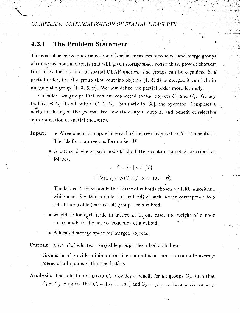
4.2.1 The Problem Statement

The goal of selective ~naterialization of spatial measures is t o select and merge groups

of connected spatial objects that will, given storage space constraints, provide shortest

time to evaluate results of spatial OLAP queries. The groups can he organized in a

partial order, i.e.. if a group that contains objects (1. :3, 8) is merged it can help in

merging the group (1, 3, 6. 8). \Ve now define the partial order more formally. - -

Consider two groups that cont rlin connected spatial objects G', and G',. \Ve say

that C;, 5 G, if and only if C;, C G,. Similarly to [:3S]. the operator 5 inlposes a Y

partial ordering of the groups. We now state input, output, and benefit, of selective

rnateri3alization of spatial measures.

Input: a i'b- regions on a map. wherc each of the regions has 0 t o .\' - 1 neighlmrs.

The ids for map regions form a set 31.

- 0 A lattice L where each nocle "of the lattice contains a set S described as

follo~vs,

S = { s l s c * Z 1 } -- - (VS,, A~ E S) ( i # j + s, n s, = 8).

The lattice I, colll-esponds the lattice of cuboicls chosen by MRt; algorithm.

while a set S within a node (i.e., cuboid) of such lattice correspo~ltls to a

set of mergeable (connectecl) groups for a cuboid.

a weight ~c for e ch n ~ d e in lattice L. In our case, the weight of a node Q corresponds to the access frequency of a cuboid. ,-

Allocated storage s p x e for merged objects.

Output: X set T of selected mergeable groups, descri bed as follows.

Groups in T provide minimum on-line con~putation time to compute aL7erage

merge of all grotips within the lattice.

Analysis: The selection of group G, provides a benefit for all groups G,, such that

C;, 5 G,. Suppose that C;, = {u , . . . . .a,} and C:, = {a l . . . . , n,. a,+,. :. . .a,+,}.

* The benefit B;, of merging group G', with respect to group Gj. is expressed as

follows.

B , , = mergr-fimc({al.. . . . u, ,+,)})-~ncr~c-t ime({{al . . . . a,}. o,+l.. . . . n,+, 1 *

Given a lattice L of dimensions. each being associated with a benefit value B and

a weight value kV, find a fixed number Ii of dimensions to merge: such that the total

cornputatio~ial time using the merged clirnensions as a hasis in the computation. is

mini~nized. d

This problem is intractable becatise it can he recluced from set-covering prot>lenl. v f

Thus. we prspose several heuristic strategies.

4.2.2 Spatial Greedy Algorithm

As we csplairiecl in C'hapter 2, the no st widely used algorithm for the select iGi of

cuboids for niaterialization is the NHl i , a greedy algorithni presented in [:HI. A-21tl~ough

I this algorittm perfonlis well in the creation of a conventional (nons~;atiaI) data cube.

it callnot hc) applied for handling spatial measures. Therefore, we propose a new

algorith~n that ~naterialiies only selected cells in the cuhoicls choseh by the HRt'

algorithr~i. Note that each cell contains a group of pointers to spatial objects. \.1

also refer to this as a group of spatial objects. The folloiving heuristics are used for

selection of groups of corinectecl regions ~o hc prernergcd.

nccess frequtncy

Based o n the access history or the estimation of t,he access frequency of a set

of nodes, one can ca.lculate the benefit of the merge. If a group of connected

regions is more frequently accessed than other groups, it is more beneficial to

prenlerge (an& save) this group of connected regions.

cirdinnlity of cr o f c o n n d t d regions

If a candielate group has more coi~nect~ecl

beneficial to select this cancliclate in the

during on-line processing). Xotice that L

regions than other groups, it is more

premerge (having fewer disk accesses

i f a merge is performed on a set. of

conne.cted regions at. a descendant node, the subsequent cost analysis on its

ancestor nodes sho~dcl count tire newly merged region as one region only. *

4

0 sharing among the nodes in the cube lattice ~ t r u c f u w . -

If a candidate is shared among more nodes in the lattice structure, it is.more

herieficial to select this candidate for premerge.' Notice that in this case, the

access frequency of a group i s the sum of access frequencies of all the nodes in

which the group appears.

Based on these heuristics. a benefit formula is worked out to compute the total benefit

of merging a group of connected regions. The total benefit is the sum of dilvct bfrzefit

and indtrwf brntfit. The former is the benefit generated by thc merged group itself

due to the recluction of' both the accessing and merging cost (since no merge neecls 0

to be computed at the query processing time); whereas the latter is the benefit of

tlic other groups in the ancestors of the node containing thgpremerged group clue

to their use of prenlergetl group, which reduces accessing and on-line computation

costs. Ascentling t'he lattice of cuboids leads to more general clescriptions of data

in the database. Subsec~uently, if some objects have same nonspatial descriptions in

one cuboid, they will have same clescriptions in all ancestors of that cuboid. \V 'e now

introcluce a term notz-occludd ancestor.

Definition 4.2.1 Let F and C: be groups containing pointers to spatial objects such

~ 6

that C; c k'. Then. group F is a rton-occludtd ancestor of C;, C; -i F , if the following

-_ conditions are satisfied:

a group F has not been nlaterializecl

a there is no materialized group J such that G c J c F

there is no materialized group J 3 J c F such t,hat G n J # 0 mtl cardinalityl./)

The following formula& compute the total benefit of premergirig a group G:

clirtct-bene f i f ( G ) = cicccss- f requcncy(C:) x cctrclinnlity ( G )

total-bmc f i t ( G ) = direct-bene f i t (C:) + iaclirect-beae f it(C;) (2.3) I =

The For~nula (2.1) indicates that the direct benefit of a group C; is the product of

its access frequency and its cardinality, i-e., the number of regions to be merged. This

is derived based on the following observation. For a group containing k regions to he

rnerged, if it is merged into one region. the cost of each access is t o fetch the merged

region once. 'Howe~er. if the group were not merged into one region, it woulcl take

about k unit accesses to fetch these k regions, perforrn on-line merge, store the result +

into a temporary file. and then take one unit access to fetch the merged temporary

file. Thus. the merge saves about k unit disk fetches for each access. A

\I;hiie the access frequency and the carcli~lalit; of the connected group of spatial

ohjects contribute to the direct benefit, sharing anlong nodes in the cube lattice

structure contributes to the indirect. benefit. In order to determinc the inclirect benefit

for a group G, we have to consider all groups that contain group C. By prernerging fA

group C;, we effectively clecrease the ca.rdinality of all its ancestor groups. If a group

cont a im A- cormectetl regions, prernerging its suhgroup that. contains n regions ( n < k ) ,

decreases cardinality of the group by n - 1. Formulx2.2 shows that only 11011-occlucled

aricestors of a group C: contribute to its indirect he~iefit. The following esample

illustrates camputation of the indirect benefit. B

Example 7 Let A = (1, 2, :3,1, .5)..B = (1. 2. 3, 5), C' = { I , 51, D = (2, 3. 4) . and

E = (2. 3 , 4. 5 ) . and F = (4, 5) be six mergeable groups. MTe explain the following

five cases that can occur when calculating the?ndirect benefit of group D.

1. there are no materialized grodps -

Since group D is contained within groups A arid El both these groups contribute

t o the indirect benefit-of D. e

.- 2. only group E has already been materialized

There are no groups that contribute t o the indirect benefit of group D. Both A

.and E are occluded ancestors of D (E is ~naterializecl and D c E c A) .

:3. otily group C has already been materialized 1

The indirect benefit of D is the same as in case 1, because groups C and D do

riot intersect.

4. only group F has already been tnaterialized

The indirect benefit of D is the same as in case 1, because even though groups

F and D intersect, the cartlinality of D is-larger than the car<linalit~. of F'.

5. only group B has already heeri materialized

Only group E contributes to the inclin~ct I3enefit. of group D. Group '4 is oc-

cludecl group R. since groups B and D intersect antl the cartlinali~y of B is

larger than the carclinality of I).

After t hc. nicrgeable canclidatc groups arc- detected, the greedy algoritlirri proceecis - as follows. 111 tlic first round, the algorithm computes the total benefits for all can-

cliclatc groups, compares their txnefits, and selects t he oric with t he highest I~encfit.

In subscyuer~t ro~~nt l s , the benefit estimatio~i may change for soriic groups since these

groups may contain tlie sul3gronps of the rnerged groups in the previous round(s).

Tfic hcnkfit for these groups will be updated antl sr~ch updates will propagate up r - along the lattice. I he adjusted benefits are compared among the remaining candi-

dates and t h e one with the highest current benefit is selected for tlic prenierge. This

proccss continues until it completes tlie maximum number of allowable merges where

the maximum ntmber of merges can be determined based on the allocated disk space.

or other factors.

Based 011 the above outline, the algorithm is pscsentecl as follows.

Algorithm 4.2.1 (Spatial Greedy Algorithm) A greedy algo&thm which srlrcts 0

candiclatr (connected) region groups for yemerging in the construction of a spatial

data cube. .

Input: a .A cube lattice which corlsists of a set of selected cuboids (presented as

~iocles) obtained hy runrii~ng a cul>oitl-selection algorithm such as H R I J [:3S].

a An access frecpency table which shows the access frequency of eadh node - - [

a2 in the lattice. J

a A group of spatial pointers in each cell of cuboids in the lattice.

a A region map which delineates the ~leighborhood of the regions. The infor-

mation is collected in an obj-neighbor table in the format of (object-pointer.

a-list-of_ neigh bom). * a rna.r.-rl unr-group as the maximum nurril>er of groups which are espected to

Ile selected for prernerge. - Output: A set of c"a"ndidat.e groupsl stored in mr,grd-obj-table, selcctetl for spatial -

prcmergc. and a spatial data cube selectively popiilatecl wit,h spatial measures.

Met hod: 5

a The niairi program is out linccl as follows.

a 'The proceclure f irrd-corlncct~cl-grouys(cor~c1idn"te Jcible) is outli~ietl as follows.

For each cuboid in the cube lattice. determine mergcahlc groups(s) in its spatial

pointer groups. by using-obj-ntighbor table. Then, calcl~late the access frequency

of ever- detected group bx su~ltniing up frecluertcks of the cuboids in which the

group appears.

CHAP TEE 4. JlL4'IERLALI;ITJ_Tf OLY CIESPSPmLL XI F,4 S TI RKS -. LPPP

* 0 The procedure s r l e c t ~ c n n d i c l 6 t e ( e c i ~ z d i c l c ~ t ~ _ t c ~ b l ~ is outlined

as follows.

(1 1 ) mcrycd-obj-table += best-group;

The functions dirtct-bsnc fitCyruup) and ind ircc f -bcnf f i t ( y r o u y ) calculate di-

rect and indirect benefit for the group according to Formula 2.1 and Formula 2.2.

Kotice that if more than one group have the same largest total benefit, the group

containing fewer vertices is 'chosen in order to generate smaller merged region .L

and save the total space.

The procedure populnte-cu be(m ergen-obj-toblff is outlined as follows. O bjects

stored in the rut rged-~bj-table are linked with the cells of the cuboids. This can

be i'nlplclnented by storing pointers, to the premerged objects. Note that more

than one cell can point to a single spatial object, i.e., a spatial object rnay be

the measure in more than one cuboid.

Rationale of the algorithm. The spritial greedy algorithm can be reasoned as fol-

lows. The algorithm works on the cuhoicls selected by the cuboid-select i o ~ ~ algorithm

HRI ; [:38]. Line (1) finds ail mergeable groups within selected cuboids. Lines (2) and

.

(3) initialize mfrgdobj-table to an empty set,, and rcrnairting-set to all connected

groups (cundidaf E-table). Line (5) presents one iteration of the greedy algorithm.

At each iteration. the algorithm selects the best candidate based on the benefit cal-

culation. The algorithm is a greedy one because it commits to a local maxi~nunl

benefit at each iteration, however, not every locally niaxinium choice can guarantee

the'global maximalit)-. .As shown in the analysis of the HRT; algorithm in [:HI, tllc

global optirnality is an XP-hard problern. Therefore, based on the similar reasoning

to that in [:IS]. thc algorit,htn derives a suboptimal solution for the selection of cancli-

date groups. Note that instead of the actual numl~er of groups ( mn.r-rt,u~n-grot~~)), the

percentage of groups to be selected for premerge can be specified.

Both our algorit hrn and t hc H R l i algorithni are grcetly a lg~r i t~hms for sclcct ivc

materialization in the construction of data cubes. Beside the difference in applicatioti Q . s

clornains: ours is on spatial data cube construction, whereas theirs is on n o n ~ p a t ~ ~ a l

ones, thcrc arc scveral other major differences. First, the IIKl; algorithm is to selec-

tively rnatcrialize cuboids ( r i e u ~ ) . whereas ours is to selcctivcly rnatcrialize particular

cclls of the choscn cuboids. This additional level of csarniriat ior~ is essential since

the nonspat ial aggregation results in sirr'iple measures, whcrcas the spatial one necds

both ~ioritrivial spatial compuitation ;ind substantial storage space. Thus. the two

algorithms are dealing with the prohlems a t different levels. Second, the HRlJ algo-

rithm does " h t t akr node access frequency into eonsideration. shereas onrs cynsiders *

it seriously. We believe that access frequency is an inlporiant mcasure since it niay

not he beneficial to preconlputc and store the rarely accessed spatial ele~nents. 9:

In comparison with the I IKIT algorithm, the selection liandled in our algorit hnl

is at a deeper level and examines every precomputed elenient in a node to be mate-

rialized. This refined computation is more costly than examining only at a (lattice)

node level. However, the complexity int roduced-here involvc~s mainly simple bmefit

formula co~nputi-tion wliich costs usually less than a spatial operation. ;LIoreover. this

conlpiitatio~i is &ne at the cube construction time hut it bill speed on-line spatial

corn putat ion or save sul)stant ial storage space, and is thus worth doing.

- .-In example of the execution of our algorit hni is presented below.

CHAPTER 4. MATERIALIZATION O F SPkTIilL MEASURES

ALL *, - - .

Figure L 5 : A lattice for the selected cuhoids

Example 8 A map with its spatial region partition is given in Figurc 4.4 and a (cube)

lattice which rcprcscrlts the relati6nships among a set of selected nodes a f ter execut ion 4 of the HRIT algorithm is presented in Figure -I..;. Suppose that the mcrgeable groups

1

for each cuhoicl wcre extractecl. \IVe show them too in Figure 4.5. Some groups that 7 -

belong -to a single cuboids may are connected with each other. but they still exist as

the separate groups (e-g.. (4, 6) and (7, 8) in cuboid r-loBoCo). This is cxplainecl

as follows. Only groupstttiat belong to same uples may be ~nergetl, because they C clescrihe thc object with same values for nonspatial climensions. Suppose the access

freqyency of each cuboid is shown in Table 4.4.

The access frequency of every candidate group (i.e., a set of connected regiop) is

equal to the access frequency of the corresponding node where i t resicles. If it resides

in more than one nocle, its access frequericy is the sum of the access frequency of all

the nodes where it resides. For example, group (4, 6 ) appears in two nodes, AoBoC"o

CHAPTER 4. ,1IATERIA LIZATION OF SPATIAL hlEAS URES -56 "

- - - - - - - - --- - - -

Table 4.4: Acccss freci~~cncy of thr cuboids

Node (cuboid)

A40&)(?o

intlir I total 1 dir I i nd i r

Access frequency 100

Tab15 -I..?: First three iterations of spatial greedy algorith~n 9

i

* - . B

- and A1 BoC0. Thus, the accormtlat~d access frequency of the groop {4. 6) is 100 +

Using the benefit calculation formulae, Table 4.5 is generated which clescribes the

process of benefit computation and premerged region selection, as shown below. At

the first iteration, starting with group Glz = ( I . ? ) , we get direct-bcnc f i t (G l2 ) = s

f reqzicncy({l,2)) x cardinc~lity({l. 2 ) ) = 70 x 2= 1 10, and inclirtct-berte = ,.l

f r t q u c n c ~ ( { 1 . 2 . 1 . 6 . 7 . 8 ) ) ~ (cordinali ty({l .2}) - 1) = 60 x 1 = 6O.'Thus the total

beliefit = direct benefit + indirect hmefit = 200. Atterition.shoofc~ be paid to t.11~ ral-

culation of the indirect henefit of some groups. Let us exanline another group. GI it; = d

'(1.4.6). Its indirect beliefit. i n d i r c c t - b t r t ~ f i t ( G ~ ~ ~ ) = (frrqtrtncy((1.2.-1.&. 7-81) + fr.cqctcncy((l,:3,-1.6))) x (c .nrd7 ' r~u l i l y ( { l14 ,6 ) ) - 1) = (60 + 120) x 2 = 360. The

largest total benefit (with a valw of 2070) is for the group (1.4.6). and that group ,

is the first selected premerging group.

In the second iteration, for some groups. such as (4. 6. 7, 's) . the total 1)rnefit will

riot he changed. However, for some groups direct t>enefi t , indirect benefit, or hot h may

change. 'Take group { 1,2, 4.6, i, 8 ) as a n example. \Vit h the merge of { 1,4,6) in t hc

first rouhd, the cardinality of { I ,%, 4,6,7, 8 ) recluces from 6 to 4. Therefore, its direct >

heriefit = .f 'r~qutr7cy({l1 2,4,6,7, 8 ) ) x cnrclinality({{l, -1,6), 2 ,7 ,8) ) = 60 x 4 = 2-40.

The indirect benefit is 0 since there is no any other larger group that can benefit from

mcrging this one.

The conlputation of the indirect benefit heco~ries more c"omplex like in the-case %

of {4;6). In the i r s t it era ti&^. { , 6 {1,3,-116), { , 7 S } , a n {l12,4.(i . i . i i} '

rrould benefit frorn merging {4,6). Horneve<, after group { 1 4 ) has been merged. 1

it occludes groups {1,3,4 ,6) and {1,2,4 ,6 ,7 ,8) . In other wortls, it is more beneficial

to use {1,4,6) than (4.6) to merge these t w ~ groups. Being the only non-occlutletl

ancestor of {4,6). group {-I. 6 , i , 8 ) solely contri butes to the indirect benefit of { l. 6) .

Consequently, the indirect benefit drops frorn 820 to 70 whereas the direct benefit is

not changed.

f the third round, the three selectecl groups are { { I , 4, 61, ('7. 8).

{A, 6) ). The pr;dcess repeat s until t,heenomber of groups selected reaches a specified

. I

h

CHAPTER 4. AfATERIA LIZATION: OF SP'4TItl L MEASliRES 58 - - - - - - - - - - -- - - - --- -- - - - - -- -

4.2.3 ' Pointer fn%ersection Algorithm

- The spntial greedy algorit hi% proposed in the previous subsection, although based d heuristics, selects good candiilates for premerge3C:nfortunately. the algorithm may

not scale well enough in a presence of many map objects, and there are two major

reasons for that :

0 All groups of spatial pointers have to be diriJec1 i i t o disjoint groups i.e.. only - regions that are connected may be derged.

A11 clisjoi~it groups are analyzed. The presence of a large number of mergea ble

groups is likely t o result in Yery expensive cornputat ion of t llc indirect benefit,

i.e., somt grottps may have a rtuml~er of non-occlucled ancestors.

Thus. we propose pointer. intcmfct ion algorit hrn that favors spatial pointer g ~ o u g s

that appear in many cuboiPds and with high access frequency. In our subsequent anal-

ysis. we assume that a set of cuh/ids*have been selected for materialization using an

estendecl cuboid-selection algorithm similar to the I I K U algorithm. \\::'e now examine V heuri:tics to determine which sets of mergeable spatial objects should he preconi-

puted. The general idea of the algorithm is as follows. Given a set of selected cuhoids

each associated with an (estimated) access frequency, and min-fr*eq ( the niinirnuni

access frequency threshold), a set of mergeable objects should he precomputed i f and

only if its access frequency is no smaller than ruin-frcq. Xotice thati a merged object

also counts as t o be accessed if it, is used to construct a larger object. Only after

the intersections among the sets of ohject pointers are computed and those with low

access frequency filtered out, does the algorithm examine their corresponclir~g spatial

object connections (neighborkbod information).

The y o i n f f r intersccfion algorithm is outlined as follows.

Algorithm 4.2.2 (Pointer Intersection Algorithm) A pointer intersect ion met-

11ocl for the selection of a group of candiclate connected regions for precomptation

and storage of the merge results during the construction of a spatial data cube. w

Input: A cube lattice which consists of a set of selectmt ettt3oIrts obtafrmk by

running an extended cuboid-selection algorithm similar t o the HRU algo-

rithm [:3S].. The selected cuboids are mapped to a sequence of numbers

from the top level clown.

An access frtqufncy tuble which registers+the access frequency of each

cuboid in the lattice.

A group of spatial pointers (sorted in increasing order) in each cell of

cuboids in the lattice.

A region map which delineates the neighborhootl of the regiorls. Thc infor- 5. #

mation is collectecl in an obj-rtcighbor table in the format of (object-yointfr.

rniri-frtq: A t hresholcl which represents t tig mi ninial access frequency of a

group of connected regions to be prernerged.

Output: A sct of candidate groups. stored in mtrgfd-obj-tnblc. selected for spatial %r

premerge, and a spatial data cube select ivdy populated with spatial measures.

Method:

0 The rnai~i program is outlined as follows, where rnn.r-cuboid is the masinlun~

numbcir of cuboids selected for materialization.

FOR cuboid-i = 1 T O rnct.r-cu,boicl DO

FOR cuboid-j = cuboid-i T O mar-cuboid DO

FOR EAC'H*cell-i I N cuboid-i DO +

T h e procedure yct-mn.r-inters~ction ( i . c b o d j cnndidak-table) finds the

maxinxd intersections between the cell cell-i and all cells within the cuboid

cuboid-j. It is outliaecl as follows.

(1) PROCEDURE yet-rnc/ ,r- ir~tcrstct ion(ctI l i , crtboicl-j, candidate-fciblt ) {

r 7 I hc fuiictio11 y ~ t - r r ~ ( ~ . r - i n t ~ ~ s t c t ( c ~ l l - i , cell-j) can be in~plcmelitctl as follows. Set

two cursors. / I , arid 11,. pointing t o the star t ing positions in c f l l - i and cell-j

r e s j x ~ t ively (wliere object pointers a y sorted in ifircasilrg order). If both

cursors point t o t lie identical objcct, out put tlic. pointer to t tie resulting buffer

a11d forwasrl hot h cursors. 0 t herwar , forward t Ire cursor which points t o the

srnaller pointer. This process repeats until one of tlie cursors reaches the end of &

t lie set. 'The output is tlie resulting buffer. *

Note that irtcifr*i-cnn(lictatf (intersrctcd- ort ti on, candidafc-tnblc) inserts the in-

tct:s.tctcd-portion into the cnndidntr-tablt i f such a portion is nonexistent in the

table t,oget,llcr with cuimid ids. If the intersected port,ion is already in the can-

clitlate table. only the new cuboid id(s) i.s insert,etl. ii

Thc procecluri. f r tqc~f ncy-co~nputing-€/'-filt t ring or tit did at t- tnblf ) is out 1i11etl as

follon~s.

- - - - - & -

CHAPTER 4. OF SPATIAL MEASIiRES

Table 4.6: Access frecpencies of selected cuboids

is examined for each candiclate cube cell which derives the maximal intersections

of spatial object pointers and stores t&rn into candidate table. Note that a self-

intersection for cuboicls is performed as well. Line j.5) removes from the candidate

table those canc1ida.t~~ whose total access frequency is s~naller than min-freq. Line *

(6) finds the spatially c&nectcd subsets within each candidate f a group of pointers

to spatial objects) ancl line (7 ) materializes them and puts into the nlcrgdobj-tnblr.

Optimization has heen explored in each proceclure/function. For example. proccclure

gc t - rr tns - in fer .~~~c . t io~~ . checks one cell ctll-i against cuboid-j, by first finding the first

candidate cell in cuboid-j and then cstracting the intersected portion. Afterwards the

intersected port ion is renlocecl from cell-i since there is no man: such portion in t hc . remaining cells of the cuboid. Z

Note. tVe now clarifj. t fie reason for applying the self-intersection in this afgorit h m . I

(Lines (1) ancl ( 2 ) ) , sincc it might not be obvious to a reacler. There can he a rlurnbcr *

of groups that appear in a single, yet frccjucnt cuboid and it is important that such

groups be identified. Were a self-intersection not applied, these groups wo~llcl be

skipped. The performance analysis. conducted in Chapter 5 , will show that thc self- s

intersection has a significant positive impact on the effectiveness of t,he algorit hnl (see

Figure 5.6).

\ Example 9 111 order to illustrate the exrcut ion of this algorithm. we revive the exam-

ple used for the rough nttasurcs algorithm. The map (Figure 4.3), the lattice showing F-

selected cuboids (Figure X2). and the sets of pointers for selected cuboicls (Table 4.1)

are identical like in Example 6. Let the the access frequency of each selected cuboid

be as shown in Table 4.6, arid let ntiit-frtq threshold be 40.

.After applying steps depicted on Lines ( I ) to (.1) of the algorithm, we get a set I

of cantliclatcs in Table 4.7. Raw access frequency of a candidate is a sum of the

CHAPTER 4. ,bf A TERIA LIZ TION OF SPATIA I, MEA S IJRES 9

Tottal access frequency

4.5 t - 4.5 t 4.3 c: 65 t 6 5 c 6.5 t 6.5 +-

65 t 3.5 -

:3.5 :j

3.5 :j 5

Raw access Accumulat ecl access frequency frequenc?

Table .1.7: C'andiclat e-table for select cd cu hoids

4 5 -1 5 4 5 6; .5 5 0 50 6 5 5 0 :3 5 :f.j '

13.5 3. j 3.5

frequencies of all cuboids in which the canclidate is found as a 111iximal intersect~on.

For example, candidate {I , -1) is detected as a ~1axinral i ~ ~ ~ e r s c c t i o n between cuboids

1 and 3. so t11at its raw frequency is 50. Kote that (1. 1) appears in cuboid 2 as well,

but not as a maxi~nal intersection with any other cuboid ( (1. 4, 7. 20) is a nlasimal

intcrscction between cul>oicls 1 ahd 2. while (1, 1, 13) is a masinla1 intcmection

between cuboids 2 and 3). On the'other tiapd, the candidates that fully contain a

certain group contribute to the accurnulatecb access frequency of that group. The

accumulated access frequency of (1. 4 ) is 15 (access frequency of cuboid 2). Notice 3' .

that a single cuboid can be counted only o$ck in the calculation of the frequencies. * 1

Finally, total access frequency is the stml df rkw and accumulated access frequenciw.

The canclidates whose total access freyuefiry 'is not below the threshold are shown

0 0 0 0

1 5 1 7 5

0 1 5

- 0 0 0 0 0

with an arrow (t)? To make Table 4.7 smaller, we do not shoy self-intersections in

this example. Since mirr-fwq threshold is larger than threshold for any of the cuboids,

none of the candidates resulted only from a self-intersection can he merged. 4m

?tfter applying syafirtl-conrtfcfiviig-ftstirtg procedure, we detect that the following

regions: { 1, -1, 7). (1, 4). (2, 3) . and ( 6 . 9) (Table 4.8) should be merged. At the first 9,

Table 4.8: Regions to be prenlerged

glance, it seems that it is wasteful t o store both (1. 4) and (1. 4. 7) since the fornler

is a suhset of the latter. ~oweveri ' if both have high access frequency. it is beneficial to

store hot,h for the fast response (avoiding on-the-fly spa,t,ial merge). XIoreove~-. ot,trer

on-the-fly spatial merges may also benefit froni storing both groups. For example, { I ,

2. 1) may use the precon~puted (1. -I), whereas (1, 2. -1, 7) may use (1 , 4. 7).

C

tr 4.2.4 Object Connection Algorithm

In this subsection we present object connection algorithm, that is only slightly different

from pointt r. in t~rsect ion algorithm. \;l;hile the pointer. interwfction algorithxn first r

contputes the intersections among the sets of object pointers, and then performs

threshold filtering and examines their spatial object connections, the object conn cct ion

algorithm examines the correspondi~lg spatial object connections hefore threshold

filtering.

The object connection algorit,hm is exgnlinecl in the following.

Algorithm 4.2.3 (Object Connection Algorithm) Thh o6ject connection method

for the selection of a group of candidate connected regions for precomputation and

st,ora.ge of t'he merge results during the construction of a spat,ial data cube.

-? Input: The same as Algorithni 4.2.2.

Output: The sa.me as Algorithm 4.2.2.

Met hod:

* TPe main program is different from that of Algorithm 4.2.2 a t Line (-1) where

connection is checked im.rnediately, before proceeding fnrther. Thus. the old

Line (6) is removed since it has been clone in Line (4). . f

'*

(1) FORcuboicl-i= 1 T O mas-cuboid DO

(2) F O R cuboid-j = criboicl-i T O mar-criboid DO

( c c l l i , cuboid-j. candiclute-connected-obj-t(~blt ):

( 5 ) f rcquc~lcy-conzputing-&- f'ilteriny(cctnclidnteronizectecl-obj-table):

(6) . shc ired~.~pat ia lmergi1~g(cnnct ic1ci t t~co~~nected~obj~tnblc .

nrerged-obj-tablt ); L*

s

(7) populcite _czib~(nzcryed-obj-tnble);

P

r Since only the procedure yet-mc1.r-conlztct~d-ilztf rstction (cf l l - i , cuboid-j, cnn-

*

didnte-connected-obj-table) is different-from the procedure yet-~nnr-intc~wecfiorl

of Algorithm -2.2.2, it is o t r thed as below. Other procednws are essentially t h e A

same arid thus are not presented here. s

( 1 ) PROC'EDITRE gc t-?ncc.r-2o~~r~ect~cl-i~tttrsectio~z

(cell-i , cuboid-j, candic la te~connectcd~obj~table) { 1 -

( 2 ) cell-j = yet- f irst-ceEl(cuboid_J); a

C3) - r e n ~ a i r ~ i n y - c d l i = cell-i;

(4) WHILE ( I r ~ m a i n i n y r e l l - i > 11 A N D cell-j # 8) DO { '

(3 ii~tersectecl-yortior~ = yet-mcis-intersect

(remaining-cel l - i , cel l - j ) ;

( 6 ) IF ~ir~terse~tecl-~ortio12~ > 1

(7) THEN insert-connecttl~l-canclidate (ilzt~rsectecl-portio~z, candidate-table);

(8) r t n ~ a i n i n y r e l l i -= i n t c r s t c t edpor t ion ;

(9) cell-j = yet-next-cell(cziboicl-j);

Note tbat the only difference from Algorithm 4.2.2 is a t Line (7)"which calls in-

sert-connected-candihte rather than insert-candidate. The procedure insert-co-

nnected-candidate (intersected-portio~i, candidate-connected-obj-table) breaks the

inter=wcttd-yoriion into a set of connected portions, by checking the obineighbor

table. Each connected portion with the length greater than 1 is insertecl into

i t h e candidate-connectedobj-table i f such a portion is nonexistent in the table.

In this case, its combined access frecjuency should be the surn of cell-i's and

cell-j's access fre~~uencies. If the connected portion is already in the table, the

access frequency should be accu~nulated. CI E

Rationale of the algorithm. The ma jo r difference of this algorithm from the former LS

one, Algorithm 4.2.2, is a t handling of connected objects. The former delays the.

connectivity checking after min-freq threshold filtering, whereas this algorith~n does

it a t the insertion into t candidate table. By looking a t the algorithms, one rrlhy * think that they produce ictentiral ~esu l t s in terms of selected regio~ts for pwnerge. 11-1

the subsequent discussion we will show that it may not always be the case.

Suppose that A and B are two groups detected by get-max-intehect procedure. *b Moreoc'er, let us assume that both groups contain a common connected subgroup

6. In the case of pointer intersection algorithm these two groups will be-checked

for spatial connectivity only if their access frequencies are no smaller than min- f rq

threshold. On the other hand, if we apply object connection algorithm-, groups il

and B will he divided into mergeable (connected) subgroups. Thus, group C will-be

inserted into candidnfe-connected-obj-tdblc. Its total access frequency tan be h i ~ h c r 0

than that of gro?~ps A and B, since it can appear in 14ore cuboids (union of cuboids - ..- for A and -B). Thus, it may occur that neither A nor B pass frequency threshold (in

e

pointer intersection algorithm) and that C does pass frequency threshold (in object s

connection algorithm). Note that the group C does not get detected in pointer inter-

section algorithm, unless A or B passes the freqsency threshold. Therefore, pointer P bL

#

iAfr .wction algorithm generates a subset of groups generated by object cone tction

algorit hrn. IVe -now provide a more forr~ral explanation. -

Theorem 4.2.1 Let PIG be a set of groups selected by the pointer intersect,ion

algorithm, and OCrG a'set of groups selectecl by the object. cpnnectionalgorithm. IVe *

c1ai1n illat P f G C OC'G.

Proof. We first provide a proof that each group in PIG must be also in OCC;.

According to the algorithm -1.2.2 each group $9, 5' E PIG'. must consist of con-

nected regions arid its access frequency must pass min-fieq thresliolcl. C;roup .C will

bc also det ectetl by i11.w r ~ c o n n t c t ~ d - c n n d i d c ~ t t procctlure of algorithm -1.2.3 and later. E

clrw to its st~fficient*acccss frcqumcy will be sclectcrl for t l ~ c premcrgc. Thus. P I G is

a su b+t of* OC'G.

Now, we prove that relation PIG = OC'G does not always hold. ---

I x t C; = GI. G 2 , . . . Grr he groups of spatial pointers fo111it1 in more than o ~ i c cuboid

(i.c., intersect ions) with the following properties:

For all groups in G, there is a common su1)group ,5"iliat consists of connected

regions.

There is no group outside C; that has S as a subgroup.

The total access frequency of every group in C; is below min-frtq threshold.

Xssunle that group S does not exist anlong iritersectecl groups i.e., it is riot clctcctd *

in proceclure gtt-mctx-intfrsection of yoir~ter intrrsecfiort algorithm.

Due to insufficient access frequency. none of the groups in C; will he put i r i P I P

group. In addition. group 5' will not be detcctetl h- -/ algorithm 4.2.2. On contrary.

group 5' will be detected by in.5er.t-connected-ca~zclidnt~ procedure of algorithm -1.'3.:3.

The set of cuboids cuboid.s(S) in which it resicles is

1=1

Since the access frequericy of S is higher than that of any group in G. group S may

pass the frequency t hresliold ant1 become a member of O('C;. '

1 - -- - ' CHAPTER 4. MATERIALIZATI,ON -- - - OF - SPATIAL - M E A S U R ~ S - - - - -- -- - - - - -- - -- 68 -

Table 4.9: Candidate-connected_ohj table for selected cuboids

- 5

*

Therefore, there may be some groups in OC'G that do not appear in PIC. This . conclucles the proof. 17.

In addit ion to its effectiveness, object connection algorit hrn has different efficiency

than pointer intersection algorithm. This will be studiecl in more detail in the-following

chapter.

Connected intersect ions

(1: 4, 7) (2, 3 ) (6, 9) (17 4)

{l, 4, li3) {12,15}

For the same example as for pointer intcrsecfion algorithm, the execution of Al-

gorithm 4.2.:3 is presented as follows.

Raw access frequency

4.5 6.5 6 5 .5 0 35 3 5

J

Example 10 The execution of Lines (1) to (9) of Algorithm 4.2.3 will lead to a

set of candidate connected object pointer groups as shown in Table 4.9. Note that

Accumulated access frequency .

0 ,

0 0 15 0 0

the algorithm finds same maximal intersection groups like Algorithm 4.2.2 (see col-

83

Tot a1 access frequency -

45- CU

65 +-

65 +

6ri e

:3 5 35

umn "Intersected-port.ion" in Table 4.7). After in.sert-connectecl-cnndidnfe procedure

is executed for each of the intersections, we get candidates shown in "Connected

intersections'' column of Table 4.9. Similady t,o Exa,rnple 9, the access frequencies

are computed and frequency filterin@ applied. Candidates that pass the frequency

threshold are marked with an arrow (t). The marked groups are the regions that

are selected for premerge. 9

Since Examples 9,and 10 contain only a small number of objects. the two algo-

rithms produce identical results. Our performance analysis will show that the case

described in Theorem 4.2.1 occurs very seldom, and that i t has a small impact on the

benefits of selective materialization.

C H A P T E R 4. P

A2fATERIA LIZAT'fON OF SPATIA I, l\IEL4S URES - - -- - - - - -- --- - -

69 - - - -

C

ri

e

* -

a' "

4.3 Utilization of Spatial Measures in On-Line Processing

Clearly, there are Jhree main tasks in the life cycle of a spatial data warehouse:

crt'ition, usage, and maintenance. The focus of this study is the process of creatiop

of a spatial data wareltouse. However, we devote this section to the usage df a spatial . data warehouse, gr more precisely, the usage of ~naterialized spatial nieasures. So te

that the issue of dhintenance is not stucliecl i n this thesis.

Earlier i n this = . t ljesis. we elaborated tlhree met hods for collecting spatial measures,

riamely collection of spntinl pointers, apyro.rirnntc corrtputcrtiotz of s p f icil rn~asurc.s', =a

and .sclccfim mnt~r icd i~n t ion of syczticrl mrasurrs. While, the measures collected by

the first method can be utilized similarly t.o tionspatial (r~umorical) measures, the

latter two met hods need more discussion.

Iltspitc having cliffcrent accuracv and thus tliffcrcnt objcctivcs, both rcppro.rirrtntt- *

comp~~tnfior2 of synticil mtnsur.es, and . i ; t l w f i ~ ~ rncitct-i(diSatio~ of spccfial rrifccsur~s,

popi~late only portions of the cuboids in t>he spatial data tube. While the first niethocl

eliminates rlierged ibIE3Rs with low nrtcrx~ight . the seconcl one filters out tricrgecl --

regions whose niaterialization is consiciered to provide little benefit (while wasting

st oragt space).

4.3.1 Utilization of Estimated Spatial Measures

Estimated, or roughly calci~latecl spatial measures provicle a user of a spatial data

wai-ehouse with an insight into nonspatial and spatial properties of objects on the

map. Althoi~gli they can scldon~ be used for final decision ~nakiiig, t h e j can help the

user focus on the particular seg~nents of the map. To ~ n a k e a clecision support process

more f ru i t f~~ l , we suggest the implementation that allows users to clynamically change

the area-ul~iglzt t hreshold. hIoreover, we believe that approsiniatc con~putation of

spatial measures slioulcl serve only as a coarse grain tool.

\

IVith a large number of frequently used spatial objects precomputecl and stored in the

merged-obj-table, it is interesting to see how to find the best carlcliclate set stored in

the table for efficient on-line processing, For example, suppose the rncrged-obj-tnble

stores the following s& of merged regions: (1, 4). (1: 4. 7). (2, 3). and (3, 8, 9).

A measure cell derived by an OLXP operation may have the following set of spatial

pointcrs: (1. 2, 3. 4, 7. S, 9). A smart search algorithm may return two precomputed

(merged) regions: (1, 4. 7), and (13, 8, 9) . with one additional spatial merge, (2)

+ { : 3 , 8._9), done on-the-fly. Howh~er, an unintelligent algorithm may return two

prcconiputecl regions: (1. -I), arid (2, :3), with three aclclitional spatial merges. (7) + r

{ 1. 11, (8) + (2, 3) + (91, done on-the-fly.

At the first glance, one may suggest t o first match the prcconlputccl regions con-

taining t h z largest nurnbpr of 'rner ed objects, then proceed to those with smaller 5 number of niergcd objects. Howevcr, this may not always work wcll. For esample.

supposc the ntcrytd-obj-lnblf contains (1. . . . , 101, { 1 , . . . . 11). (1 1, . . . , 20). a11d

(12, . . . . 1-11. and the targeted measure cell is (1, . . . . 20). If we first select the

region containing the most elements, the result will be { I , . . . . 1 l ) , and { I % , . . . , 1 4 ) .

H o w r r r , the selecti611 of { 1, . . . . 10) and (11, . . . , 20) is a better choice.

11.e Iia\+eethc foll'owirlg technique for the selection of precomputecl spatial ohjects

for a target T , which c o n h t s of a set of spatial object pointers, representing a spatial $3

measure cell resulted from a spatial OLAP operation. Let -21 be the rncrgfd-obj-tnble . . B

1. Create table S such that , S = {s I s f 121 A s C T). Notice that an element

of n~crgccl-obj-table .U is also the element of table S , if ancl only if, it is fully

. contained within the target T: If T is a large set, an index can be constructed

on ,\I and/or S for efficient search.

2. Search S t o find all the maximal groups C; such that

-.- B

C ; = { ~ ~ ~ E S A ~ C T )

Table a4.10: Canclidates for selection of premerged spatial objects IC

Xo

1

*

This is inrplenlentecl by finding the first match y 5 T , estracting f . and then C

rtct~rsivcly repeating for T - g.

XI1 rriasirnal groups G are stored in the pool of carldidates T.

Set of premerged objects

{1 ,2 ,3 ) ,{4 .7 ,8 ) ,{5 ,6 ) ,{9 ,10)

* 13. For each group C; E I' calculate the follotving parameters:

cot~rngc: number of objects in C;

Coverage

10

0 n urn-n f-prtconlp t~tcd-objccfs: number of prenierged groups in G

rlurn-of-on-lirrc-WE rgts: numl~er of objects that have to be rnergecl on-the-

Nun1 of premerged objects

4

fly in orctm- to eumjrttte the, target T.

/;*lrarly, the following equation holds: f* -

Nun1 of 011- 1i ne merges -

4

4. Among all groups in r select the group with the s~~la l les t value for ri urn-o f-on-li-

Example 11 Supp&e,a spatial measure cell res-dtetl from an OLAP operation con-

tains the following set of spatial pointers: {1,2.3,4,.5.6,7', S,9,10}. Assume that the *

search of the rncrgerl-obj-tablt, !\I (Step 1) finds the following set of precomputed t

objects: 1 2, I } 1 2 , 3 4 3 , 4 5 , 6, 7, S } 4 , 7 ' 8 , 1.5, 61, {7. S, 9, lo}, {9,

10).

r

F CHAPTER 4. !bIATERI.4LlZrlTIONOFSPATPAL MEASURES

Step 2 derives the sets sf candidates, shown on- 'Table 4.10. In Step -1 gsoap No. :3 - - is sclerted ;is the answer since only three objects +haveF$o be mcrged on-the-ff y. . + - * -

r - - 2. 0

%

Chapter 5

Implementation i and Experiments

This chapter consists of two parts, the prescntation of GeoMiner: a system prototype *

for spatial data arid mining, and the esperiment:al r r sd t s of our research. Since

the GeoMiner system prototype has resultecl from a joint work of GeohIiner Research

Group rncrnhers, the author of this thesis will focus on his part, 0 ,LAP engine, a~it l its

importance for data mining modules. Since 01113. a portion of the presented rmearc-11

has heen i~nplementecl in the GeoMinsr system, a simulation-based perforniance study

was conductecl.

5.1 Design and ~rn~lernentatikn of the ~ e o ~ i k x system B,

B The GeoMiner system [36] is an exteasiori and evolution from a relational data min-

ing system DBMiner [:35] researched ancl developed in Intelligent Database Systcrrls

Research Laboratory a t Simon Fraser University. At the present time the DBMiner ' system contains the following five data mining functional moclules: charactt rizer, conk-

pamtor, nssocintor, classifitr, ancl prrdictor. Several additional data mining motl~iles, " s

including mining from time-related data. are at research'and development stage. \Ye

advis the reader to look a t numerous publications that esplain DBMiner structure I and its data mining techniques [:32, 33. 34, - 3.5, $3, 441.

CVe are aware that data mining is unsupervised learning, and that a user has to

direct the discovery ,prociss. Therefore, an import ant isstte in designing and devel- -- - oping a data mining system is providing a user with an easy and a straightforward -

way to formulate his/her mining requests. Due to our belief that the success of rela- s,

t ional clat abases shoulcl be' crecli ted in part t.o the creation of _the stanclarclised cluery

language - SQL, we suggest that tzh6undrrlining structrlie of a proposed data mining

language he SQL. In addition to espressing mining recluests, in the form of rules, the

proposecl language has t o handle spatial predicates. such as clovt to . *contairrs. inttr-

. \ F C / . ~ . etc. We suggest a GMQL - Cko-Mining Query Language [:Ti'] foi- fornlulati~lg f

mining requests.

:\ti aclc uate presentation of discovered knowlcclgc is yet another significant issue _ 9 for a data mining system and <Iealiiig with spatial data adtls cvcn more importance

to it: Only if spatially-1~1atcct knowledge is vistializect. can it he interesting to a

knowletlgc worker. ('onsecjr~ently, we tlesigned and implerni.nted various visualization

tools for all types of discoverqcl. kn

5.1.1 System Architecture I

The GeoMiner systcm i s co~istrtlcted on top of the DBMiner system. AIining of noli-

spatinl data is directed t o the DBMiner s\.-stem; whereas mining of spatial data and

t hc. relat ionships I~ct w e n spat ial arid nonspatial data arc perforrn>tl by the tlctlicatecl

Geominer functions. The general afchitecture of the GeoMiner system, presented on*. &

-

Figure 5.1, f&ttires five ini its: Y -

- .1. A set of cliscoverl\- moclules tlmt includes: gto-chrirctcierix r, geo-gorrrpcirn tor. J

3

r /r o - n a s ~ i n t o i : gro-clrrait r a ea l~yxi : and yco-rlnssifier. \k plan i o develop two-

' aclclitiolial modnles: gco-prtdicfoi- and gco-pnttcrn .antrlyxr. - 9

* 1 Z

2. .4 data cube mining ettgine based on DBMiner discover- kernel for mult itli~rlcn-

3. A spatkt1 datahase servervjnclu~led within Mapltifo Professional 4.1 G e o p p h i c

Informat ion System. +

b

Z

I Graphical User Interface 1 +

%

Ceohliner: Discovery Modules -

I Spatial Database Server and Data Cube I

e i Figure 5.1: General architecture of G e o l I i ~ ~ e r

1. .A graphical us& interface for interactive data mining and for display of mining

results in the form of taljles, charts. maps. etc.

5. The data-. and knowledge-base, storing nonspatial arid spatial data and their

concept hidrarchies. 5.

The functionalities of the five esisting discovery modules are outlined as follows.

Geo-characterizer finds a set of characteristic rules atnrnult,iple levels of abstrac-

tion from a relevant set of data in a spatial database. It provides users with a

multiple level and a n~ultiple angle view of the data in a spatial database. Ry

using this rnodde t h e following question, for example, can be answered: '.C;ircn -&

spatial hicrarchirz o j tht Cnitrd ~ t n t r . s . ~ a h a t a r q c n r r a l income pntirrns oc-

cording to rtgion partitions?".

- .*.

.f: -

t 3

t'MAPTE& 5. fLWP&E;%E~YT+TM Aftr;E, E X m m T - S - - - 7 6- * i *

Geo-comparator discovers a set of comparison rules that &nt,rait the general

-features of different classes of the relevant sets of data in a spatial database.

It compares one set of data, known as the tnryet class, to the other set(s) of

data, known as the contrasting c lass (~s ) . For example, this module may show

the digerences in migration patterns in the United S fates . or find thc clusters

dr fcafur&s relatedto the Eoccltions which diflerentinte the profiting stores frorn

-the non-profiting orzas. *

Geo-associator extracts a set of strong spatially-rel-atecl association rules from . i -

a relevant set of data _in a spatial database. An association rule @~ows the f

frcqucritly occurring patterns (or relationshipsj a database [4.9]. .A t ypkd spatial

association rule is in the form of .'.Y -+ 1- ", where -Y and 1- are set)$ of spatial I\

and/or nonspatial predicates. For exan~ple: an association rule can reveal thc

+ ~ ~ l n t i o n s h i y s bf tzrwn golf cour-sc.9 und o t h t r nrnrby objects l ike parks, roads,

Iclkfs. ctc. It

v,

c

-$ Geo-cluster analyzer uses an efficient algorithnl C L A ~ . A N S [54] to perform spatial

clustering. After it detects clusters, gto-clu.sler rcnnlyzer finds nonspatial descri+p- -

tions of the clusters by usin8 the attribute-oriented inductioh n e t hod [:31]. For

example, one can find how tirf .$tares rrrf clus[ertd nnd thcn, find &scriptions

for fach cluster to dctcrmint approprinte marketing s f m t e g i ~ s .

Geo-classifier adopts a generalization-based decision tree induction method to d %

built1 a clAssification tree that classifies a set of relevant data-according to one

- , of the nonspatial attributes [-MI. The classification tree is di~played and by

clicking on any of the nodes of the trees user highlights corresponcling region(s) , :- *

on the map. For example. one may clns.s~fY stairs i n thr ljnited Statra nrcording -3

f o the mcrlicln family ineorne in a state.

The data rninirig modules clescri bed above use spatial database server to est ract Z - 1

data relevant to the data rn in ingPhces~ The spatial database used for the irnplr~nrn- '

tat ion. Maplnfo Professional. provides a connection to many external databases using

- * B

ODBC' functionalities, import of data from other spatial data formats, and querying 9

of spatial d a t a using native version of Spatial SQL.

The data retrieved frorn the databases is analyzed by clata mining modules. The I

data cube underlying architecture enables fast manipulation (roll-up, drill-down, .$tic-

ing, dicing) and analysis of large amount of data. The multidimensional data analysis

utilizes concept hierarchies. which are stored in a_tlatsal;a:;e. With the ascension of - a co~tccpt hierarchy. informat ion becomes more general. but still remains consistcrtt

with the lower concept levels. 'rake occupation concept hierarchy as an example. Both

\%.TI drs ign c rlginft r and sy.stcm.l; f ngincer can be gen~ralized to concept comput fr

c l i i c ip turn can be genrralized to concept rnginrer. *which includes n t f - *

chtcntcctl t ngirlrfr. as well. A sirnilar hierarcffy may exist for spatial clata. For example,

in a gcnernlEtion process. regions representing counties can be merged to states and

states call& merged to larger regions. Concept hierarchies can he built based on

the e x p t ~ t knowledge br, in the case of nunkesical concept hierarchies, created au-

tomatically. The relational concept hierarchies nre stored as tables in a relational

cla t t&se. The spatial concept, hierarcl'lies contain precomputed spatial aggregat ions a &

to. accelerate data analysis process.

Y 5.1.2 Implementation of OLAP in the GeoMiner System

One of the essential features pf GeoMiner is its ability to"perfor111 multilevel spatial t

data mining and spatial data analysis. Data in spatial databases usuall- ccnitains

detailed information a t the primitive level of abstraction,- also known as mu^ dotn. It

is desirable to summarize a large cjuantit,y of clata, and present it a t a high ahstractiori

level. Ebr exanlple,given climate clata for a region, one may want t o summarize this

detailed clata. and present the general characteristics of the region's climate. Such a

process woulct generaliie - raw data into concepts like colcl, mild, hot (for temperature), *

dry. u ~ t (for precii>itation j. etc. Portions of the map (regions) that are tlescri bid

by the same high level concepts can he merged together. However, with a blind.

gerieralization, data may h e surnmarizecl to too high a level, and provide a common

sense knowledge. Thus, we stress the interactive and nlultilevel pqradigm of the

The system provides not only the power of generalization (roll-up), but also the

power of specjalization ( drill-down). Wliile*roll-up or reduction of a dirnensibn is a

.. relatively simple concept, drill-clown requires more explanation. One may ~vontler . '

how a drill-down-operation can be performed and whether it introduces an additional

- level of complexity. Obviously, it cannot be accomplishec~ by working directly on

a high level cul>oid. A value, once geseraliztul. cartrtot be restored witl~out being , . 0

mycd - bcforch~ncl-. -Therefore. we maintain a bnsf cuboid. also known as the Ecc~st

ijc~~cr.nlistd Cuboid. kVhe11 clrilling-clown to a spccific cuboid. we effectively roll-up

from tlic lmsc cuboid. In addition to typical OLAP operations on nonspatial data.

the GeoMiner system allows for OLAP on spatial tlata,*.also known as spatial OLAP.,

Thc OLAP conipollcnt of the GeoMiner systeni cogsists of two modules: chomctrr ixr . *

arid compnrator. that prodi~ce c h n r u c f ~ @ i ~ a541 =cornp riso11 rules respectively. \\f

\now cwmirie these types of rules in more detail by going through two examples.

p t t rh- in thr i7nitcd Stotrs by presenting the reIatialsIiips among the regions wit tl

;;o rcspect population s i ze .~mdian family income, a ~ l d percentage of people holding \

This data mining request can I)c forrnulatcd with the followirlg GMQL "-

query. \

ANALYZE s ~ n ( ~ o p ~ ~ b

WITH RESPECT TO gee. st,at,ena,mc.

FROM states-census " b

WHERE time = 1996 -d

First. thc system retrieves t h e data related to nnmc of the stnte (statena~n;). *

population (pop). median family incornc-f rneclfamincomc), percentage of pol)-ulation

holding bachtlor dfyrce (wit hhachelor,degp). and with time being t h e year 1996. G f o

is a spatial attribiite that corresponcls to a niap object.'

Figure 5.2: Display of spatial characteristic rules.

13asetl on thc~ giver] yucry and the spatial conccpt hierarchy for gco attrihutc

and ~lonspat ial concept hierarchies for pop. nlect_Earninco ancl wit h-bachelor-tlegp

attributes a spatial-dominated. generalization is performed '"a a follows [5:3].

Spatial-do~~iirlatc>cl generalization triggers the merge of the connectecl regions, artel

creates a set of larger merged regions. Effectively, spatial clescriptions of states, gfo ,

are generalizecl into larger regions li lie IVE ~ L J England, itTirlrllt -4 tlnntic, :Yorth Cent rcd, i etc. Xscenclirig t h spatial concept hierarchy leads to fewer objects. Generalization

of the spatial objects continrles until the spatial gt ncmlizr~tion th rvsllold is reached.

T h e spatial generalization threshold is defined as , the maximum number of regions in

a gcntr.alittd rrlafion. C;encralized relation is a table that uses generalized values for

attributes ( a table a t the right-harid side in Figure 5.2) . -

I

After the spatial generalization process is performed, the rtonspatial data is re-

trieved and analyzed for each of the generalize objects using tRe attribute-

oriented induction method [:32]. Three main attribute-oriented induction

technique a're:

1. climbing the concept hierarchy when attribute valu&s in a tuple are changed to

the generalized values 1 ' I

2. removing attributes wlken further generalizatbn is impossible andfor there are

too many distinct values for an attribute

3. mqrging itlent ical tuples

'The induction continues until a value for every attribute is ge~ieralizecl t o the.

desired level, specified by the yenemlization f h reshold for that attribute. During the

process of merging identical tuples, the number of merged tuples is stored in additional

attribute count t o enable quantitative presentation of the acquired knowledge. In our - r

example. sum of population for states in merged regions is also stored to enable

presentation of the measure ' ~urn fpop ) ". Notice that a single spatial object can be

described by rnttltiple tttples i~ a gene~itli-zed relatiort. This is the result of having

different rlonspatial clescriptions for objects that generalize. to the larger object.

The above process creates a generalized map of the I_i~iited States (Figure 5 . 2 ) .

However. we believe that a t this moment, fruitful arid ipteractive OLAP is yet to '

start. Drill-down or roll-up can he performed interactively on such generalized data

t o zoom-in or zoom-out the generalized spatial regions or to examine the detail; of 3

their associat,ed nonspat ial properties. Invoking roll-up an& drill-clown OJAP oper-

ations fetches the cuboids from the lattice of cuboid&. The fact that the cuboids

contain rnaterializd spatial nleasores*greatly enhances* mining a t niultiple levels of

abdraction. Figure 5.3 shows the resu1t.s after drilling-down along spatial dimmsion

to present details describing the southern part of the llnited States. The results car1

be presented in the form of a two-climensional chart, pie chart on the map. and a

generalized relation.

CHAPTER 5. IMPLEMENTATION AND EXPERIMENTS

Area of a ple presents value of "sum[popSOl"

43,566 853

mlh-bachelor-dew-0-13 wlth bachelor degp-13-17 with-bachhelo;degp-17-22 w~th-bachelo;degp-22-31 w1thIbachelo<degp-31"or-rnore

Figure 5.3: Drilling-down along spatial dimension

In the presented example, mining is performed by generalizing first along the spa-

tial hierarchy. Then, this process triggers the attribute-oriented induction process on

nonspatial attributes to describe nonspatial properties of generalized spatial regions.

Therefore, such generalization is called spatial data-dominated generalization [53 ] .

Alternatively to spatial data-domin,ated generalization presented in the above ex-

ample, nonspatial data-dominated generalization can be performed if a spatial concept

hierarchy is not given. This method includes the following steps:

1. Collecting all data relevant to the query.

2. Applying the attribute-oriented induction on nonspatial attributes, i.e., gener-

alizing to higher concepts. For instance, median family income values in range

(10K : 20K] can be generalized to poor.

3. Collecting pointers to spatial objects that are described by the same high level

nonspatial concepts. These pointers are put in generalized tuples. Again, the

g tncmt i x f i on threshold is used to determine when to stop the generalization

process. - f

-1. Potential merging of neighboring objects that belong to same generalized tuples. * I

The results of this process can be visualized in the form of thematic map which

present regions according to t,heir generalized rionspati81 clescriptions. We now de-

" scribe the last step in a little bit more detail. In some cases. merging of objects that \r -

_ are compact enough (e-g., states) i not necessary arid would only add to the overall

complexity. Thus, the current version of the GeoMiner system does not perform such a

merge. If the merge operation is t o be performed; it could be signifi~antly accelerated

by preconlputing and storing the rnost frequently used spatial aggregations (merged

regions). - -

Example 13 Suppose that a w e r wants t o find the migmtion yntf trns in the t*nittrl

Stntts, and to compare regions with large increase in the population from 1980 to d

1992 and regions where the pop~la t~ ion clecreased during the same period. This data

mining request can be formulated with the followi~ig GMQL query.

MtNE COMPARISON

AS "Ibligrat ion Patterns"

ANALYZE supl(pop)

WITH RESPECT TO geo, statename.

pop. crimeslOOOOOR, mcdfarnincorne

FROM states-census

FOR "Significant-populationincrease"

WHERE p o p 8 0 X P > 20

VERSUS -'Populat ion-decrease"

WHERE pop80_9Z? < 0

The query compares the two classes of objects with respect to spatial location

(geo). narnt of the state (statename), populafion (pop), ratio of crimes per 100,000

yroplt (crimes100000R). and nz~dian family incorn6 (ntedfamincome). -

4

* - To process this qu&y. the system first retrieves the relevant set of data from

8 - the relation states-census. The collected aata is part itionecl into three contrasting

B

classes: "SigniJiccrnt-population-increa.s€"," Pop ulation-decrease", and "Others". The

~'Siy~iJicant-populntion-incr(ct~s~'~ class contains states where populatio* b e h e e n 1980 6 and 199% increased by more than 2056 (ivliere popS0-92P > 20). The "Populn-

* tion-dtcrense" class contains states where population decreased i r ~ the same period*

of time. Finally, the '.Othtr.r;" class consists of objects that do not belong to ei-

ther one of the first two classes. The objects be%nging to the contrasting classes %

arc generalized to the same levels of concept hierarchies. Then, roll-up. iri~l-&u*,, .

and alirt operations can be applied a ~ c l ~ r o n o u s l y on all classes. Cknekliiation alld C

, * - 4

specialization are perfoimed ba;rd on the hierarchies associated with the following cfi-

mensions: spatial dimension (g to) and four non-spatial cli~ncrisions: sfntrnnme;-pop, *

crinrts100000R. and nwdfanl:incornt. The nieasores contain two values. count as, the

default nit-asure and sunr[p:p) to present sum of population in particular regions. An

esamplc of t he result of the conlparison query esecutiori is presented i n Figure, 5. W -

5.1.3 ~ g l e of OLAP in Spatial Data Mining B

Presefitation of summarized data is o111y one of the reasons for rforrlling spat id OLAP operations. Xiore importantly. we see OLAP %s a tool that enhances spatial

f-' - data rniriing. Previously, we briefly described gfo-nssocintor. geo-clusttr c~nrtlyxr, arid *a p-" -. &*

yto-clrt.ssifi6 r modu1i.s. The attractiveness of these mining modules is at their ability

to discover multilevel knowledge from a spatial tlata base. When performing either

generalization or progressive deepening it is essential that the respo&e time be small. - *

Linderlined tlata cube technology provides the GeoMiner system with a reasonably fast

response time.

CHAPTER 5. IMPLEMENTATION AND EXPERIMENTS

Area of a pie presents value of the count

S ignificant-population-increase Population-decrease Others

Figure 5.4: Results of a comparison query

5.2 Performance Analysis of Proposed Algorithms

In Section 4.2, we presented three algorithms for selective materialization of spatial

measures: spatial greedy algorithm, pointer intersection algorithm, and object connec-

tion algorithm. In order to evaluate and compare their effectiveness and efficiency, we

implemented the algorithms and conducted a simulation study.

The simulation is controlled by using the following parameters:

0 number-of-objects on the map. Since the only spatial data type that we discussed

so far is a region, the map is comprised of regions only.

0 mas-number-ofineighbors for an object.

number-of-cuboids selected by the HRU cuboid-selection algorithm [%I.

min-number-of-tuples as the number of tuples in the most generalized cuboid.

e mas-fwqnt ncy as the maximal access frequency of a cuboid.

4) yew-o f-gronps to materialize (for spatial greedy algorithm).

min-f ir(-mtio as the ratio (for poinltr intersection/objcct conntctiorz algorithm)

between minimal frequency ttireshold'and average access frequency of all cuboids.

llinimal frequency threshold is used to filter out groups of spatial objects that *

hav6 low access frequency. Specifying the frequency thresholcl is done in an

indirect way. \;e enter a ratio between the threshold arid the average cuboid 5

freq~tency, because it gives more control over the simulation.

33- k\'e 11ow espIaln the major steps of our simulatiori.

1 . Gencrat ing a map.

A map is created by specifying values for n u r n j o t arid mar-n umber-of-

_nfighboi:s.. WP do not takG into account size of the map objects (regions) and k-

" the riuniher of \-ertices.

2. Sct t ing up a spatial dat a warehouse.

\t'c create a spatial data warehouse by specifying three parameters: nurn-

bcr-of-cuboids. min-rt urr~brr--of_t ~ p l ~ in a cuboid, and max-nurnb~ r-of-f up1f.q in

a cuboid. Being primarily concerned with spatial measares, we do not compose

values for diniensions, and numerical measures. Instead, we generate a set of rt,

pointers to spatial objects for eaEli tuple i n each cuboid. In addition each coboi<l

is assigned a rando~n frequency in range (0:rna.r-frequency].

3. Selective rriatcrialization of spatial measures.

\k'e choose and execute an algorithm. For spatial grefdy algorit hrn we specify a

value for pc rc-of-@ouys to be materialized. whereas for the other two algorithms

we specify a value for min-freq-rat io The chosen Falgori t hni selects

groups of spatial pointers to be in a spatial data cube.

4. Simulating typical OLAP operation on the spatial ctatja warehonse. - We simwlateposing of queries t o the spatial da ta Garehsuse. Here, we use cuboid

c, ef 9 frequencies generated beforehand. We also pose queries that are infrequent (do

not appear ia the set of selected cuboids).

The map. content of tuples, and cubnids' access frequencies are generated ran- '

don~l~~fo l lowing uniform distribution. We believe that other distributions should not \ . - significantly affect the relative performance and thus would lead to similar conclusions.

-

+ Tie simulation was performed on a Pentium 200hIIHz rnachine running iVindows NT

* 4.Q operating system. The sirnulation code was written entirely in hficrosoft Vis~ial

' C+$ f .2.

In our-presentation of all three algorithms, we assurnecl the esiste~iceof obj-ntighbor

table that-aselerates checli i~~g connectivity of objects on the map. However. creation J > . .:d such a table is likely to take some substzmtial processing effort anel thus there is an.

a+ option to perform neighhorhoocl test directly on the map objects.

We divide our pcrfor&nce atlalysis stridy into two parts. First. we analyze fit- f i r -cn~ss of the algorithms. Since the goal of selective matc4alization is to enhance

on-line processing, we study the usability of n~atcrializccl groups. IVe are interested in

knowing (1) how much on-line processing time is clccrcasecl by performing off-line pre-

.conrputation. and (2) what is the storage ov6rhead that such precornpiitat ion yields.

Secon"c1, we conipare qficienry of the algorithms in terms of precomputation running

time. Although precomput.ation running time is not eve11 distantly as crucial as on-line

runni'ng time, we are still congernecl with pre~omputation efficiency. The main reason

for this concernFis maintenance of a spatial data warehouse. Even though spatial 3 -

objects may not very fregucntly change, their nonspatial a t t ri hutes can change. Since

we consider merge of objects with same nonspatial descriptions, updates of measures

(both spatial and nonspat.ia1) may be quite frequent. S

5.2.1 Effectiveness of the Algorithms

k! In this subsection we examine effectiveness of the proposed algorithms. We are mainly

b interested in deternlining the benefits that precomputatiorl generates and the resulted

- P

CHAPTER 5. Ll.IPLEI\.IENT,4TIOAr A N D ESPERnilEiVTS , 8 'i iX-;

storage overhead. We now define a few terms used throughout the subsequent analysis. - - Pi, <>

. L scilying in the number o f disk ncc f s ses -

5 -: The goal of materialization of spatial measures is getting short response time

- - ..g for OLAP operations. If 11 spatial objects are to be merged during on-line . .processing it woulcl take n + 1 disk accesses t o read n ohjects and store the

iL

resulting - mefgecl object. If these n o b j ~ c t s are premerged only one disk access

(read) is needed. hioreover, since we focus on computation bf spatial measures *

c we count only disk accesses t o objects that are t o be merged f ,r in the above +

e example). Note that these objects may be original spatial objects or already - 7 - preniGrged objects. I hu;. we define an,.iny in th t ks,rrbc F o f disk ncre2ars as

?p the pcrccntage of disk accesses that are avoided~(11ot necessary) due to off-line 0 -5

Ifaterializat ion of spatial Incasurcs ~ n a f yiclcl large storage overhead. i l 'e present

s t o r n y o w r h f a d as the ratio between total storage space neeclccl for spatial

measures and the space for the original m a p objects. %

IZ'c first analyze spcct i d g,verly algoritli~n in isolation, because of its different stop- .

pingcr;terion from that of the other two algori=thrns. Figure 5.5 shows the cffectivrll&s

_ df spcltinl greedy algoritlinl. The figure illustrates the benefits of selective niaterializa- d . - - tion, expressed as saving in the number of cbsk accesses duripg on-line processing.

S

Sote6 t !iat in this experiment we considered only OLA P queries whose results are e.

(partiah1~~)~niateri~lizecl (chosen by the M R U algorith111). Later in this subsection we . . - will examine OLA P quEries that are not chosen by the HRt r algorithm.

The slope for the benefit curve in Figure 5.5 decreases when*the numbrr of mate- -,

rializedgroups i~jcreases. Our explanation to this is that the initial prenierge obtains t

i large boo& due to that many of the merged regions are shared by diffrrent nndrs - - and that the premer& leads to a relatively'hig rerl~~ct&on rat icv on 'the sizes of the

A r merged nodes. Such initial materialization really betlrfi ts man? subsequent OI,X P

ope~atipns. b'hen a certain proportion of all mergeable groups is materialized. the - . can<lidates with such nice features may have been used u p and the benefit becomes

- trend. T h c colicretc savings-and when the satur:atiort point is rcachc~tl can be only - I

nii rie the nt111lhcr of p r ~ m r ~ r g e d grot tps. ; \ rcording~t~- t he:?$ pe r immt clrscrilml above.

tlie materialization of a sniall portion of groups leads t o ~efiso'tiahly good p ~ ' r f o r n ~ a ~ i c e - i

in lerrns of t h e t rack-off I,ct\set~rl response t ime and t be storage space. ?

f P y .

The remaining two a lgor~thms. yoint fr , i n f r ~ x c f i o n and objfct connection, a re s

compared with respect t o their effectiveness in Figure 5.6. Here. we analyze benefit I

as a furlction of rnin-jreq-rxtio. i ~ ~ ~ r o i l u c e t l % 9 earlier in this settion. The figure reveals a t he following:

T h e brief i ts of both algorithms decrease with t h e increase of f s e g u e r i ~ thlesh-

0 Therc is o& a slight tliffererict. hefween effectivenyss of the two algoritllms.

If self-;ntersectiorl is not a i lp l (~d. the brnefits d o not converge t o 100%.

%

z

: C'HA P TER 5. IMPLEMENTATION AND MPE R~~VIENTS - -- - -

7

F i p r e 5.6: - rialization

Pointer int@rwction and object connection algorithms: heriefits of mate- 9

* It Lvas exp&trd that a higher requency tliresliold lvatls t o tlie smaller iinniher of J/ premrrged objects arrd thus t the smaller benefit. Like in tlie rasr of spatial g ~ r ~ d y

algori t hrn, benefits for these two algorithms convergG to 1.80%. ( redch lOb% percerit C

wlie~i no frequency t hresholcl. is applied). - - The slight difference bet ween effect ivencss

of pnirrlf I i n t r rscctiora and object connection algorithms follows from Theorem 4.2.1.

The tliffercncc is more or less r n a r g i d in o ~ ~ r sirnulation, flowever only the real world

application with a large n~irnber of spatial objects can corrfirnl a potential irenil. -

,.As we explained in our presentation of pointtr'ir~tfrsrctiorr a11d object cdnneclion

algorithn~s, perfdrrning t lie self-intersect ion on cuboids vastly inlproves the henefi ts of

niaterializat ion. If the self-intersect ion were not app-lied, a t most 77% of disk accesses

would he avoiclert during on-line processing. When the frequency threshold incr6ases I

the ctiffc.rences hecorne marginal.

\1P used the results gathered in the previous two e x p r i r ~ ~ e ~ l t s t o compare the

e~er t iveorsb of all three algorithms. The objectiw of this perlorn,ance study was * to rlrtermine which algorithm selects best candidates for premerge and under wllicll

conclitions. In order to compare all three algorithn~s, we had to find a common

clenominator for the algorithms. and the natural choice was dorngc oaerhend. Note .

0 50 100 150 200 250 300 350 400 t storage overheadw]

- .*+ Figure 5.7: C'orriparisori of algorit hrns: benefit of materializat ion

that storage overtleael iy ltot all i ~ i p u t paranieters fur ally of tl ic. algoritlirns.

r 7 r i t i l ~iow. i w 11ave lookecl a t benefits of precornptltation for partially or fully nia- -

tt~1~ia1izc.d cuhoitls. i.c.. chosen by the H R l i algorithm. ~ V C J arc. in atltlition, interestctl

in irnprovi~ig the rcsponse tinie for all ot&r OLAP queries ( those that arc riot c3vcn '

jects can inlyrove their response time. Bei~k rnainly intercstecl in spatial measures ~ v c

created orily grotips of spat,ial-pointcrs as 511- answer t o a query. T h e n t~mhcr of such

queries was as high as 100,000. a

Figure 5.7 shows that : - - * = 1

0 For materializecl cuboids, spatial grtfdyalgbrithril reaclirs the saturation point

faster than the ot,lier two algori t liriis do. *

* 0

Pointfr in&rst.ction and obj~cf connt.cfU)r~ algorithms arc better at t;antllirig - a

non-matcrializcd cuhoicls.

This is analyzed as follows. First anel foremost. it is important t a realize that

poitlff I- inffrsfcfion and object conr~ecfiorr algorithms select caricliclate g r h p s from a.

- = -

larger pool than ..spe#iat gmxly algorithm does.- Let us illttstrate this witk a sinlpie eF-

ample. Suppose the group (r-l.B) appears in two or more tuples (in different cuboicis), dc

hut is always accompanied bfsome other connected o b j e ~ t ~ s . Thus, this group will not *

be detected by the greedy algorithm !groups like (A ,B , . . . ) will be detected instea'cl), b

but it may be an" intersection tetween at least two cuboids. On the other Ilarid ever- &

4 .

rnerg&ble group extracted&% the greedy algorithm, is also a self-intersection of a

cuboid it belongs to. - f'onsequently. pointrr int~r.wction/object connlzctiort aIgorithm selects a riurnbes

*

*

of sniall cartlirplitj- groiips* that are corn~ion to a riurnber of cuboids., Note thct a -* -

premergecl object-may be used for answering an OL.-ZP query only i f it is fully q m -

tained in onc of the resulting tuples (it cannot be containccl ~i'itllin more tlian one - tuple fos a single query). Since premerged objects are con~putecl on the basis of ma-

-

tcrializetl cuhoitls (chosen lq fhe HRLi cuboid-selection algorithm), all these o1)jects

are legitimate candidates for a k v e ~ i n g at least Xhr query. In grnrml. pssmrrged ob- - jects consolidatctl from a large number of ~r ig ina l nlap objects are h e t t ~ r cancliclat~s ..: - -+*-

I- - than the s~ ia l l c r ones. Thus, by riot selecting ' r 6v cardinality groups syntic~/ gretdy * *,

algoritlim utilizes st omge better than the otlicr two xlgorithrns (lo- For the above rea-

,sons, spnt idyr .c fdy aigorit hrn outperforms pointtr inter-section and objcct ronnfction t -

algori t h~ns, in answering the' OLAP querics whose results are ntaterialize&

Exactly the opposite happ6ns when the queries whose results are not, materialized

are posed. The likelihood of fitting large (in terms of inner carclinality) prenlerged s

ob&cts into resulting ones is small. Thus. i t is more beneficial to use F11ia11 objects

gene;ated by yointcr inierscction arid object conncc n algorithms. This esplains the 9 bottom part of Figure 3.7. However, t 6ere is an issue of accessing premerged objects

that may not be overlookecl when considering non-materia1ii;ed queries. The access - 1 *

t o spatial measures of a materialized cuhoid is fast clue to a highly i;idexihg structutp * v

of a-spatial data cube. Answering to non-materialized queries requires search for

best candirlates a~riyng prernergetl objects. Note that cubbids for such queries are

not created off-1i1k. Intuitively, premergecl objects can he organized in a hierarchical

structure such as R*-tree structure. Nonetheless, further reseztrch in this direction is . '"

C

necessary. J

- Another observation from Figure 5 7 is that curves fur pointer ia tersect i~n and

object connection algorithms intersect. This simply shows that additional objects

(see Theorem 4.2; 1 ) premergeclL by the latter algorithm are not 'alw%ys verf useful for < v - .-q

on-line processing.

The aboveanalysis leads to the following conclusion: If only queries with material-

izecl results are to be run againgt the spatial data warehouse. spnttgl greedy algorithm - I

should he used. On contrary. if there is no specific pattern in the usage of the data , r%

wnrehottsq and there are few queries whose res-ults are materialized, pqintrr -interscc-

tion or ob t c f . connection algorithm should be used. W7e believe that latter conditions

arc more realistic in a real world application. 0

B *

5.2.2 Efficiency of the Algorithms *

The fact that spr~tinl grt-trly algorithm has different stopping criterion than the other '%

two algorith~ns do, makes us unable to st.rictly compare efficiency of all three algo-

rithms. Thus. we first discuss the efficiency of spatin1 gwcrly algorithm and tlien coni-

pzre the efFiciencies of yointrr intersection ancl object connfction algorithms. Despite 9

this limit ation, we will suggest the fzvorable conclit ions for each of the algorith~ns. We

- that these two parameters are signi$icant in our simulation study, hut also and Inore

importantly, they are vital for a user of a spatial dat~.wareliouse. In all experiments.

we fix the fol'lowing parameters: 11 umber-of-neighbors = 10, min-~tumber-of-ttlples = e

I

5, ma.r-n untber_of_t up1e.s = 100, rrbar- f r e q u e r ? c ~ 1000.

Figure 5.8 shows the execution time as a function of nuniber of objects in the - - s

database. In this experiment we fix. the number of cuboids to 10. We can see that

spntinl greedy algorithm is very sensitive to the number of objects in the database.

, + Since we asSume that each cuboid covers the whole map, the simulator generates ( n u r n -

her-of-objtcts '/ mrrs-n urn bt 1.-of-tzlplts, n u r n b o f b j c t / mirl-n uniber-o f - t z ~ p l ~ s ) &-

jr'cts for eycry tuple. Thus, the first *step of the algoritlim,~detection of mergeable

groups is very expensive ancl it creates a large number of groups. Having a large

t i

- , - i-

cL

r

CHA P T ~ R 5. IMPLEMENTATION AND EXPERL~IEIVTS .. . 93 , * - * d - f - - - rp -- - ---- -- -- - - - - -

P - C - - - -

*

\ 5 , -

100 150 200 ' 2 5 0 300 350 400 450 500 number of objects in the database - - * -

1

Figure 5.S: $calahility of spatial greedy Blgorithm as a f u ~ ~ t i o n of number of map I *

objects . -

10 15 20 25 30 35 40 number of cubold$in the data cube

Figure 5.9: Scalability of spatial greedy algoritl~nl as a function of number of cuboids

number of groups does not only increase the number of iterations in the greedy algo- * *

rithm, but also prolongs the execution of each iteration. Note that benefit for every

unmerged group has to be recalculatetl in every iteration of the greecl_v algorithm. - Sot sur risingly, execution time has linear growth with the increase of percentage af 2

9 grotips ( ycrc-of_groups) t o be materialized.

Figure5.9 shows the scalability of the algorithm when number of c u b i d s increases f l

( the number of objscts was set to 100). The performance of the algorithm is like in

the previous exp~rirnent. Thus, we-conclude that spatial g i w d y algorithm is equally

sensitive to the number of objects and the number of cuboids (views) in the data L

e

cube: Later, \ve will see that this property makes the algofith~n very useful under 5 cert air1 confdi t ions. 9 .

\Ye now focus on the k n a i n i n g two algorithms. Figure 5.10 shows the . . r

-?2 - -

C'HA PTER 5. I~WLEIUENTA ?ION AND EXPERIiMENTS 94 d

L- , - - - " ---- - -- - - - - - -- -- - - -- - - -

7 - - - - - - - * .

a ' P i

- * ' a

a >

.I - 9%

100' 200 300 400 500 600 , 700 800 900 1000 number of objects in the database -

Figure 5.10: Scalability of pointer intersection and object contiection algorith~ns as a fur ic t io~~ &nuinher of objects %"

I .F *

comparison of the algorithms when they are applied on maps_with different nwnher of

of ohjccts is small, objtct connection algoritlitn has anfetlge over p6intcr intersection

algoritlirn. However. by increasirig the n~~rf lber of objects, the p e r f o r ~ n a r ~ e of object

conrirctio~, algorithm significantly deteriorates, while yointcr intrrscctiorr algoritIirii ,

5

slio~vs little sensitivity to the number of objects.

This is a~ialyzecl 2 s follotvs. The first step of both algorithrns is firidirig the iu-

tersecting groups anlong the tuples in the cuboids, After the ir~tersectirig groups arc -

detcdecl, yointtr intrrstction algoritlm filters groups with low access freque~ic~.. 111

order to perform such a filtering, the algorithm has to cletect the total access fre-

quency of every grolip (see mar-frrquency function in Algori t hnls -1.2.2 -a~lcl 1.2.3).

3% The total frequency is a sun1 of tli'e raw frequency and the accu~rxulateii frequency.

Computation of the accuniulateci frequency of a group is a very cxpensivc operation,

since the algorit hm'has t o find all groups that contain the group. Since yointer intr r-

scction~algorit hm pesforms the above step for all intersections, there is a large time

overhead. In t.he case of object corz~tection algorithm the filtering step is post,ponecl

after connectivity test (see syntinl-connectizvity-t~sting procedure). A large number of

groups are eliminated in the conriectivity test early in object connwtion algoritlirn.

For the atxive reasofis, object con ncct tort algorit hni outperforms yoirtter inte rsection

algorithm when the ma6 contains small >umber of objects.

it'ith the snlall number of objects on the map, tuples in the cul~oicls contain 0

D

CHA4 PTER IrT, I I P L EMEAJTATION- AND EXPER4klENTS

- - - - - - -- - - -- - - - - - -- - - - - - - 6

relatively few yointm-s to * spatial objects. Consequently, cxdirlali ty of inter

groups is small too. Increasing the number of objects leads to the tuples wi u

' pointe~s. and thus to larger cardinality-of intersected groups. However, - the n 8

of intersecting gxoups does not change n~uch, and it converges to r

- i = l J = t

*

where, 31 is maximal number of intersp~tions, and tup lea(k ) is n h i b e ~ of tuples in E

cuboid Xa. * & - *.

d f - -, I'hus. the running time fdr pointtr in t f rsrc f lon algorithm only slightly inc&ases w * - ".wiih the increase of the number of objects.

A

'1

a On thc other hand, having. high cardinality groups introduces a'huge processing

ballast for corinectivity test applied to 31 intersecting groups early i r ? ob.jfcf c o n n ~ c f i o n . algorithm. Being large. many groups are split into a number of mergeable groups so b

that, t h e frequency filtering step applied i n object conntction algorithm, that contains

wax-f,v y r r f ncy function hecomes more expensive t,han the- very same step in poin t f r

minfci*.wttion algorit hrii (dealing wit,h more groups).

To ronclucie. obiid cortnccfion algoritllrn is very .se~isitive to the increase of the

rtttnlber of ot~jer ts on a map. Notice that all- cxp~rinie-nts were conducted with

obj-nrighbor table crekted off-line. %

Another observation from the curves in Figure 5.10 is that the frequency t hresholcl

is irrelevant for the execution t irne of object con nccfion algorithm. This was expected AT.

since frequency filtering is the last step in the algorithm. On contrary, pointfr 111- - tcrstcf ion algorithm shows slightly better performance when the !requenc)- threshold

increases. Notice that changing the frequency thrcsholtl does not infl.uence execution

time of costlg. ntn.r-fiquency function.

tc We now compare the two algorithms with respect to scalability to t 1 1 ~ number

of cuboids in the spatial data cube. Figures 5.1 1 (a ) and (b) show the performance

of the algorithms when applied to maps having 100 and 1000 objects respdtively.

The curves in the figdres show that objtct connccfion algorithm is superior to pointer s

intersection algorithm when the number of objects is small. The former algorithm is

(a) 100 objects 7000 I I

10 15 20 25 30 number of cuboids in the data cube

(b) 1000 objects 100000 I

10 15 20 25 3b * i number of cuboids ~n the data cube

Figure 5.1 I : Scalabi l i t~ of pointer intersection and object connection aalgorithmstns a function of numiier of cuboids

- ** veiy insensitive toethe numher of cuhoitls (with small~nurrilxr of objects). Ilowever,

*

as soon as the- numl>er of objects increases, we get results similar to the ones in _ k'igure 5.10. *

*

\Ve now analyze the observations from Figure 5.11 (a). ~ a v i n g a large number i: - i

of cu&oicts directly leads to large number of intersec-tions.' Whilc objcct conr~fction cc'I c

algorithm filters a majority of the intersection groups in its c8nnectivity test, yoiiltcr *

ir~tfrscct ion algorjitlim consiclers all the gkups in its mrc.r-Jrcqutncy fupction. If the

esprritnent were t h e wit130ut creating obj-nfighbor table off-line, perfornianccs of w F

objtct connrcl?on dlgoritbm would be-tiot even closely as good. - I t is veq- clrar that - -

crc.ation of such a table off-linc significantly boosts u p the algorithms, especially the 5

.objfct con n fct ion one. Such a '-createonce a d use-rriariy- times" n~oclcl is realistic

since i t is likely that norispatial properties of map objects will charge n~ore.frecluently

t ha11 the map objects themselves.

Figure 5.11 (b),simply confirms that pointer intrr.scc/io,r algorithm is better at

1 , handling large number of dbjects, and it can be analyzed similarly t o Figure 5.10.

We now identify conditions that favor one algorithm over the others.

0, Lire anticipate that future spatial data warehouses will bc built on the following

two premises: large number of objects and relatively s;llall number of frrcinent,.

queries. Xccorcling to the conclucted e x p q ~ j n e n t 4 ~ .a+ = we believe that pointe!. in -

t e r s~c t ion algorit h111 fits best into th i s clat@ warehouse environment. Typical &

appli'cations that corffirm to above4hsurnptions are regional weather pattern - - analysis, demographic' analysis, real esta,te business, et,c.

Conclusion

. . \Ye su~nmarizc our research work in this chaptt3r. Discufision on future dircctioris in

spctial data warehousing and spatial OLAP follows tll<slinlniarv of the research.

111 this thesis. we have studied the construction of a spatial data warehol~st. kasecl on L t

a s p a i i u a t a - cube model, which ~ons is t s of both spatial a11d wnspatial di~nerlsions - _ - 4 -- , .

and measures. wc have niade ~ iecessar~~lmdif ica t ions to t lic star sclwnia _a,

~rlotfel, (widely used for organizing dat.xwatch'ouscs of relational data) that facilitate

OLAP operat ions on the-spatial data. \ = " *

I'll* focus of our study has been on spatiadtllrasores and thcir n~aterializ?tio~i. P

\111 have shown t h j ~ t it is not wise to spatial rrleasrires 011-the-fly, however .

that rnatcrializing them all would storage needs. Thus. we have C

proposed three heuristic algorithms for kcell-hasecl selcctiv~ niaterialization, namely d - t

rit lim. The perfornlances of the algori t hnl havc hecn studied aqd ~orrlparecl with the Q * conditions listed for choosing one over the others. In addition; a method for selection

of the best materialized sets of objects from a ta,ble storirig all the niat,erialized regions

has heen outlined. \Lie have also suggested an approsirnation method ( rough r1icnsur.c~ .. 5

algorithni) for cornputat ion and storing of spatial measures.

F Currently, the methods studied fn this thesis are.being implemented in our sphtial -

data mining system, GeoMiner[Sgfgwhiclt takes spatial OLAP as the essential f ~ i n c t i o w w

' rk, module. hloreover, Gatial OLAP ope~ations b v e been iptegrated with spatial data &'

* mining moclules in the GeoMiner iysteni. 4

Ea v "c d

ct E

.. ** .o * 6.Ze ~is&ssion and Futufe Research Issues

t

I i . -. -af 0

4 .* . -

$+ The p r o p s ~ 1 algorithms and their performance study present tonvincing arguri~rnts -.

e for sclcctivc niaterialization of mergeable regions for efficient ~ ~ n s t r u c t i o n of spatial *

s n - r ~ a i a cn@s and for perforniing spatial OLAP operat,ions. Noortheless, we f ~ r ~ s e e

4% . O r 7 - h ~ r t h i~ilprovenients and exte~lsioris of t h e algoritlrnis. 1 h ~ k and some iss'l~rs that

sl~oulcl he consiclcrccl irg the future are,dut,lir!ecI below. 6

noise handling

Xlesgeakle regions, cliscussed in this thtsis, arc specificcl as the rcgi&ls that share

sorne coriimon hounclaries. FIowever, i t is soriiet imes desirahlc to ignore small

separatioris antl merge t hg' regions which are located ve4- close. I h esaitiplc,

two wheat fields separated by a highway can be cotrsidn.erl4?& orir region. This - I *.n

caw can-he trarrctfcd by mirror modifications of the algorith~~is. that treat those - '

rcgiorls that are scparatccl 114 very minor pilative) distance as rooriectecl (and

thus ~iiergeal~le) regions." @

='.

.utilization of rriaterialized spatial measures

Access to spatial measures of a materialized cuboid is fast due to-a tiiglily in-

dexing structure of a spatial data cube. liowev&, answering non-materializ~d

cuboids requires searching for best carldidates aniong precorirputecl otijccts. Ac-

cordingl~, efficient -algorithms antl date structures should be clesigncd and id;-

:e access frequency 'inforniat ion

Our algorithms for selective ma[erializat ion of spatial measures assume the ex-

istence of information about the cuboid access frequencies. IVhat if there does

not e x i s ~ s u c h information initially'? There are several methods to hatitlle this.

-t -

ne method is t o aqign initial access frecluency only to every b e 1 tn the lattice 4- - - k 1 I . of cuboids based on some data Semantics or Zssuming that medium levels are + - -

accessed most frequently. and low-levels i r e pxessed less fr6cluently than the ', t -

%'

higher ones. The frequency counts can be adjusted based on later accessing

records. Alternatively, we may choose to ~naterialize every mergeable group ac-

cessed initially. record group access frecpencies, and choose to throw away the a

later rarely used groups when disk space runs lotv. L-

. F %

0 size of the regions ,

.\ u

I! The algorithms consiclet. the access frsqucncy and-the cardiriality of t,he merge- F able groups hut not the concrete size of th? mergcable regidns. However. some *

regions could he substantially larger or inore complic~ttctl and tlius~take substm- * i

tially larger spacq and more conlputation than the others. A possible solution

(could be to acid the compression h t i o hcncfit which is the ratio in size betwqen i

th.! prr~ncrgcd and not prernerged regions. * *

ot hcr spatial nieasure operations - 7 he proposc~l algorithms aclclress Eonly the region merge operatioris in the spa-

tial measure computation. We believe that the principles discussccl here are

galerally appli;able t o other spatial measure operations, sucll as thematic illap

overlay, spatial join [30, Til]. etc. Take madoverIay as an cxaniple. If a measure

in a spatial data cuboicl represents an overlay of multiple thematic maps, such - as a l t ; t ud f and t ~ m p c r a f u r t maps, it will consist of a, nontrivial overlay 111ap

e

& .

both ill, size and effort of computation. Selective materialization of such overl&r" ?

for frecju'ently used groups of spatial objcchs seems to be essential, and thus the

studied principles should be applicable. However. the concrete algorithrns have 9 #

yet t,o be esplored. f

automa-tic gcrwratiori and dynamic acljustnwnt of concept hierarchies %i

One of the i~nportant featu'res of our research is the existence of concept tii-

erarchics and we assurnecl that they are created by users or domain experts.

However. it is preferablk to generate them autonlatically, based on the data dis-

tribution. While automatic generation and dynamic adjustment df iionspatial 9%

hierarchies have bzen studied [33], no work has been ieported on solving these

problems in the domain of spatial concept hierarchiek Farther advances in this t

direction could greatly enhame spatial OLAP, and make i t more robust. . =

a data integration

Spatial data is t l sual l~ storccl in different industrial firms and gdvernrnent agen- %

,- cies using different data formats. Data formats are both structure-specific a d a. 9

vendor-specific. There have been a lot of work on datk integration and data

exchange, but with little siicccss. These issues liave becon~e' crGcial wit 11 t lie

. emergence of:data warch~uses. . . 1

0 various applicat ion dornains

I\> believe that the principles of cell-based selective ~iiatcrialization for corii- C

putation of spatial data cubes are nat confi~ietl to spatial data oli1.i.. O t l ~ c ~ *

8 0 - _ databases which handle co1i1ple.u objects, such as nwlti~neilia-clatahascs. en-

e , r A

gineer;ng design datahas%s, will encormter similar prol~lenls~and it is rsseriti~al * --

i o perform object -based selective n~ate~ialization' as a spacr/time trade-off for

efficient O L A P-operat ions.

Several very important issues, not addressed i l l this thesis, are the efficient storage, * r

indexing. and incremental update of spatial data cubes, as well as caching of spatial

measures. Some of these problems have been estensiv$ly st urii'ecl by the (relational)

OLAP conlj~iunity. Some research results, particularly for inclesing and incrcnieri-

tal update, can be partially applied to spatial data cut>t~s. Hoivever, the seltctively *

populated cuboids in a spatial data cube, as opposed to fully populatccl cuhoitls in a s

nonspatial data cube, call for new refined methocls.

a\Vith tlie recen! success a d great p;omise of OLAP terlinology. spatial OLAP

bo!ds a high psorni;e for fast and efficient analysis of large aulount bf spatiAl data.

Thus, spatial OLXP is expected to be a promising direction for both research and &

clevelopnlent iri thc years to corne. F

i S. Agarwal. R. .-\grawal, P. 11. Deshpancle, A. Gupta, J . F. Naaghton, R . Ramakrish-

nan, arid S. Sarawagi. 011 the cornpwt at ion of rnultidirne~lsional aggregates. I11 Proc.' m

P 1.9.96 Irzt. Cbn f . l i r y Largt Dntn H N S P S . page~:i0-.?21. Bombay. India. Sept . 1996.

D. .\grawal. 1. E. Abbadi. A. &tlgli,'and T. Yareli. ~f f ie i in t view mainte~iance in d a t a

warehouses. In Proc. 1997 A C41-SIGdlOD In t . Cbnj. .Ilrcnngenzc n t of Dntn, pages X -2 i 17-27. Tucson, .-lrizona. May 1097.

N. Beck~nann, H.-P. Kriegcl. R . Schneider. and B. Sceger. The K*-tree: An efficient a'

and rofiust access method for points and rectangles. In Proc. 1990 AC'.\I-,EI(,'I\IOD Int.

C'onf. .IIrtnccycrticnt r,f Dnfa. pages 322--381. Atlantic C'ity, XJ . .June 1990. -

S. Rerchtold, D. Iieiin, and H.-P. Iiriegel. Tlie X-tree: An efficient and robust access

*t hod for points and rectangles. In Proc. 1.996 Int. C'orrj. l i r y Lorgc Dotrr Bnses.

pages 28-39. Bombay. India. Sept. 1996.

k Sons, 1996. 9

7'. Brinkhoff. H.-P. Iiriegel. and B. Sceger. Efficient processing of spatiak joins using - R-trees. 111 Proc. J99.3 A C : I I - S I C . ~ ~ O ~ ) Cbnj. .Uonngerrrent of Ilatn. pages 237-246,

Chshington. DC'. May 1993. -- - - - - -

I). t'hatziantoniou a11d K. Ross. Querying multiple features in relational databases.

111 Proc. 19.96 Int. Cbrrf. l i r y Large Dcrtrr Bmes. pages 295-306, Bombay. India, Sept.

S. Chaudhuri arid li . Dayal. ;In overview of data warehot~sing and OLAP technology.

,S'IG'.\IOD Record. 2 d '.65-7-1. 1997.

i - [9] S. C'haudhuri. R. Krishnaniurtliy, S. Potamianos. and Ii. Shim. Optimizing queries - with materialized views. In Proc. 19.95 Int. Cbnf. Dnln Engineering. pages 190-200,

w

- - ,. Taipei. Taiwan. March 1995. '

- * %

[lo] E. F. C'odd. -4 relational for large shared data banks. Cbmira~~nic~(tior~s of a4 C:.21,

13:377+387, June 1970.

[ I l l F:. F C'odd, S. B. C'odd, anitl C'. 1'. Salley. Providing OLPIY (611-line analytical pro-

ccssing) to user-analysts: A n IT mandate. In E. F'. &'orid & .:=lssocint~s (irriilablc at

f

[12] C . Colliat. OLXP, relational and multidiniensional database systerns. SIG.IIOD Rccord,

2.5:fj.t 69. 1996.

1131 K. J . Earle. Methotls and apparatus for storing and retrieving multi-tliniensional data ..

in coniputer memory. In .Arbor so f tu~~rr corporntion. I;..S. Pntcrit 59.59724, October

199-1.

[l-11 I f . Etlelbtein. Faster data warehouses. In Tech V'cb. Dcccrnber -t 1095.

[I51 11. Egenhofer. Spatial SQL: .+I query and presentation language. ZEEE Trclnsrwtiorls

011 Iirmi~lcdge h r d U~itci Enyincwirzg. 6:8Ci~95, 1994.

[IS] R . El~nasri and S. B. Savat,he. Fundarntntnls of Dutrrbnsc Systcrirs. - 2 1 ~ 1 crl. &m-

[IT] 11. Ester. H.-P. Iiriegel, and J . Sandcr. Spatial data ~nining: -4 database approach. It1

Proc. In!. Synlp. or1 Lrirgc Sp~i t id Dritr~b~~ses (SSDY7), pages'4f-66. Berlin, Ger~nany, *

July 1997:

[18] 11. Ester. H.-P. Kriegcl. J . Sander, and X. X u . X density-based algorithm for cliscovering

spatial databases. In Proc. 2nd Irlt. C'onf. on Iiriozrlcdg~ Disroz*ery

(I<D0'.96), pages 226-231, Portland, Oregon. August 1996.

[19] 11. Ester. H.-P. Iiriegel, J . Sander. and X, Xu. Density-co~mected sets and their appli-

cation for trend detection in spatiddatabases. In Proc. 3rd Int. Cbnf. on Ii~touderlgc

Discore ry and Data .\lining (I<Dfl'9 7). pages 10- 15, "Xewport Beach, California. Au-

gust 1097. a

[20] 11. Ester. H.-P. Kriegel. and X. Xu. Knowledge discovery in Iarge spatial databases: C

Focusing techniques for efficient cl5ss identification. In Pror. 4th Ittt. $imp, on Lnrge B

S p a t i d Dcttnbascs (SSD995), pages 67--82, Portland, Maine, August 1995. - I

C. ~ l o u t s o s and K.-I. Lin. Fasthlap: A fast algorit hrn for indexing. data-mining and

visualization of traditional and multimedia dat asets. In Proc. 1995 2 C'~\~-SIG~\IOD - Int. Cbnf. .IInrmgcntent of Dnta, pages 163-174, San Jose. CX. 1Iay 1995.

C'. 11. Fapyad. C;. Piatetskp-Shapiro, P. S~riyth, and R. lithurusam~,. ildzwn&s in

* E. L. Glaser. P. Des.Jarciins, D. Caldwell. and E. D. Glasser. Bit string compressor with

boolean operat ion processi~ig capability. C.S. Patedt.5036-1.57. 0:tober 1991.

.J. ,C;ray. A. Rosworth. A. Layman. and H. Pirahesh. Data cube: relational operator C

generalizing group-by, cross-tab'and sub-totah, In Proc. 1996 1,tt.l C'orzf. ort Dntn

E~~ginrrr ing . pages 1.52- 159, New Orleap, Louisiana, Feb. 1996. '

J . Gray. S. C'haudhuri. A. Bosworth, -4. Layman, D. Reichart. XI . Venkatrao. F. Pellow,

and H. Piraliesh. Data cube: A relational aggregation operator generalizing groupby.

cross- t at) and sub- totals. Dntcl hlin.irzg and I<noudedge Discomry, 1:29-5-1. 1997.

Q

-

0. Giinthcr. Efficient coniputat~on -of spatial joins. In Pror. 9th I r z f . C'orlf. Drrf(r

Engin~cring. pages 50-60, Vienna, %ustria, April 1993.

[Z] ' .A. Gupta, V. Harinarayan, and 0. Quass. Agxregate-query processing in-data warc- '

housing environmenk. In Proc. L l s t Int. C'onf. l i r y Lalgr Dutrr Bosfs . pages 358 369;

Zurich, Switzerland,' Sept. 1995.

[ 2 ~ ] -4. Gupta. I. S. 11u$ck, and V. S. Subrah~nanian. Maintaining vikws incre~nentally. P

5-

In Proc. 1999 .-1C'.\I~SIG',\IOD In&. Cbnf. .\(anugcrrzent of Data, pages 1.57-166. il'ash- -7 1 ington. D.C., May 1993. P --. I li

[29] H. Gupta. V. Harinarayan, A. Rajaranml. and J . D. lillrnan. Incies selection for

[30] R . H. Giiting. An- introduction to spatial database systems. Thc I-LDB Journal,

3:3.57-400. 1994.

., -. -

7

[31] 43. Hackatorn. Reinventing enterprise systems via data warehou&~g. In Proc. T& Dntrr

llirrehousing Institute Annsnl ~o;?ferenre. iVasbington,J).C., 1995.

I

[R2] J . Aan. Y. C'ai. a i d X . C'ercone. Data-driven discovery of rules in rzatiooal =

- %

P databases. IEEE Trms. Iinottdedg~ uncl Datn Engineering, 529-40, 1.993. 9

* a

- [TJ] J . Wan and Y. Fu. Dynamic generation aild refinement of conce>pt hierarchies for kno\vl-

edge discovery in databases. In Proc. A;Ld IP4 Clbrkahoy on Iinowlerlge Discowrg in , F

Dutctbnsrs (IiDI) 'S4). pages 1.57-168. Seattle. \VAL Ju$* @94. .t .. -

X

[&I] .J. Han awcl \I. Fu. Discovery of moltiple-level ass~ciat ion~rules f rpn large dat.abases. b\ , In Proc. 1995 Int. %Cfon f. l i r y Large .Dmtn ~ & s . pages -4.20-4.71'; ~ u r i c h . Switzerland.

$ + -

Sept. 199.5. ., "".+\. A '

44 ,i '"&

;ga7 &z+ [35] .J. Haa, 1.. F I ~ . H.. Wa'asg, .J . C'hiang, W. c;&. Ii. Koperski. D. Li, y. Ca. -4. Rajan.

- S. Stefanovii., R . Xia. and 0. R . Zaiane. DBMincr.: X system for mining knowledge in

Jarge rrlat ional [fat abases. In Proc.. 1 .!?.!I6 Int '1 C b r ~ f . on Dntn 12fining and I inou~ltd~c - Discow ry (IiDL)'9tj), pages 2.50-2.55. Portland, Oregon, August 1996.

[36] .I. Hap. Ii. Iioperski, and X. Stefanovii.. ~eoMincr : :\I system prototype for spatial - I i i n . In P m . ID87 A ( . .V-SIGY(~~~ [at. ( b ~ j . .Ikmnyemt R# ~j & t k . p;iga

5.53 -556. Tucson. ;\rizona, May 1997.

[37] J . Han, K. Kopcrski, X. Stefanovii..*and Q. Chen. Iksign and irnplen~er~tation of spatial

.- data mining engine: GeoXfiner. Subnzittfrl for piiblicntiort. .Junee 3 997.

[GX] V. Hari~larayan. A. ~ a j a r a m a n . aild J. I). I%nan. Itnplementing data cubes efficiently.

In Proc. 1896 il Clll-.YIG.lfOD %it. C'onj. ..If(in(lgt ti^ nt of Dntn, pages 205 -216, Man-

treal, Canada, June 1996.

[39] W. H. Inmori. Ilnikliltg the Data Ilicrrhousr. Q E D Tecllnical Publishing Group, \.Wles-

ley, ;2Iassachusetts, 1992.

PO] li;. H. Innion. The data_warehouse arid data mining. Conzrnzrnicatio~rs of -4 C'M, 39: 19

. [42] T. .Jo>hnson and D. Shasha. Some approaches t o index design for cube forests. Bullefin

of thi Technicctl Cbmn2ittw on Data Engineering. 20%-3.5. 1997. *

[-l:3] 51. Kaniber, J . Wan. and J . Y. C'hiang. Metarule-guided mining of multi-dimensional

*association rules using data cubes. In Proc. 3rd Int. Conj. on lin~zcledge Discowry e

nnd Data Mining (11-00'97). pages 207-210, Newport Beach. California. August 1997.

?

[-I-!] X i . Iiamber, L. ivinstone, iv. Gong. S. Chcng, and .J. Han. C;eneralization and decision - tree inductibn: Efficient classification in datz mining. In Proc. o j 1997 7nt. It'orkshop

oil Rrarrir-ch Issurs on Dntu Enginfcring (RIDE'97). pages 111-120, Birrninglmm, Eng-

land, April 1997.

-4+- I) . 21: him. H.-P. Kricgel. and T. Seicll. Supporting data tliinitig of large databases

#visual feedback queries. 11, Pmr. 10th o j Int. (bnj . on Doto Enginrrring. pages

302 313, Houston. TX. Feb. 199:l.

R . Iiimball. The Data lt7urchousr nolk i t . John t V i l v k Sons, S e w York. 1996.

R . Iiimball and K. S-treliio. IVIiy decisiori support fails and how to fis it. .S'IG,\/OI)

F:. Iinorr and K. Sg. Finding aggregate prosirriity relationships and corurtlon

bpatial data mining. IEEE Trctnsclrtioiis on ICrzordc(1ge und Vcrtcc Engineering. X:88-I-

a I i . Iioperski and J. Han. Discovery of spat ial association rules i n geographic informat ion ,

databases. In Proc. 4th Int ' I Syrnp. on Large Spitirrl Datctbclsfs (.S:!5'D '9.5). pages 47-66,. *

Port land, Maine, Xug. 1995.

Ii. Iioperski, J . Han, a11cl J . Adhikary. Mining kno\vledge i n geographic data. In Cbntin.

AC.U ( to clpprar). 1997.

R . Laurini and D. Thompson. Furrdalanw ntols o j Sprrtiol Injorprtion Sy.de rns. Acatle~uic.

1992. t

A . Levy. .A. ,\Iendelzon, and 1'. Sagiv. .Answering qukries using views. In Proc. 7th

.4 Symp. Principles o j Database Systems, pages 95-10-1. San Jose, California, March I

199.5.

LC'. Lu. .J. Han, and B. C:. Ooi. Tinowledge discovery in large spatial databases. In Proc.

Far E m f Ii'orkshop on Geogrcc~~hic Information Systems, pages 27.5-289, Singapore.

June 1993.

R. Xg and J. an. Efficient and effective clustering !nethod for spatial data mining. In

Proc. 1.994 Int. Cbzt f. Very L~~rgc D C ~ ~ C I Basrs. pages_lL14-1.55. Santiago, Chile. Se-ptem-

ber 1994.

P. O'Neil and G. Graefe. Llulti-table joins through bitrnapped joiil

Record. 2-453-11. Septemlwr 1995.

F. P. Preparata arid XI. I. 'Sharnos. ~ b n ~ ~ u t a t i o r & i l Ckomttry:

indices. SIG.\~OL)

A n In f roduc t ion.

I). Quass, :I. Gupta. I. S. Muniick. and .J. LVidom. Ilaking views self-niaintainable

for data warehousing. In Proc. 1996 Int. C'orif. P~nrdkl c u d Distributed Irlforrrtiition

Systc ms, pages 1.58-169.,M iami beach, E'loritla. December_ 1996.

S. Sarawagi. Indexing OLAP data. Rdl i tin of the Techniral C'ornrnittee on Dnta

S. Sarawagi. T~chniqncs for inclesing OIAAP data. In Ttchnirctl Report. !I?.\/ Almndcrz + '

Rrsmrch ~ % n t r r . 199i., * C

i -&-, I

A. Shoshani. OL-IP and statistical databases: Sitnilarities and differences. 111 Proc.

16th -4 Cf.ll Syntp. Principlts of I)cttrrbnse Systc r r w pages 185- 196. Tucson, Arizona,

'Yay 1997.

i

A. Silberscliatz. .\l@~nebrakcr, anrl J . D. Illlman. Database researcli: .\chieve~iients P

anrl opportunities into't he f l s t century. S1(;,2/0D Rccoryi. 25:52 63. Xlarrh 1996. - -a,

D. ~ris;ava, S . Dar. H . V. Jagadisti. and .I. V. Levy. .\ns\vering q~leries with aggregat&n . - " -

using views. In Proc. 19.96 I~t t . C h t t f . \:Erg Loryt D ~ ( I Bn.w,c, pagcs 318-329, Bombay, L _ + / * - =

India. September 1996. * . . -

$k t ~ l l h a s and .I. \Vidom. ,+I First Cbarse in Datobqrr S'ystrnz.~. Prentice-Hall. 1997.

- I

J . Widom. Reiearch problems in data warehousing. In Proc. 4th Itzt. C'orzf. on Illfor- *

nzcition nrtd h'nou9ledge ,~f~~i~cr~trizent .~pages 25-:30, Baltimore. Maryland, Nov. 1995. Ir

T. Zlfang, R. Rarnakrislinan, and hi . Livny. BIRCH: an efficient data clilsterin-g mekhod

for very large databases. In Proc. 1.996 ilCM-SIG.ZlQD Iizt. C'oizf. Munngtntrnt of Data.

pages 10:3-114, 5Iorttrea1, Canada, June 1996. * .

\r7. Zhao+ P. 11. Deshpantle, arid .J. F. Naughton. An array-based algorithm for si-

nlultaneous ninltidimensiona1 aggregates. In Proc. 1997 AC"11-SIGAMOD I d . C b ~ z f .

.\.l(mclgfrn~nt of Data, pages 159-170. Tucson, ,Arizona. May 1997