Similarity Search in Graph Databases:A Multi-layered Indexing Approach

Yongjiang Liang Peixiang ZhaoDepartment of Computer Science

Florida State UniversityTallahassee, Florida 32306-4530

liang@cs.fsu.edu zhao@cs.fsu.edu

Abstract—We consider in this paper the similarity searchproblem that retrieves relevant graphs from a graph databaseunder the well-known graph edit distance (GED) constraint.Formally, given a graph database G = {g1, g2, . . . , gn} and aquery graph q, we aim to search the graph gi ∈ G so that thegraph edit distance between gi and q, GED(gi, q), is within a user-specified GED threshold, τ . In spite of its theoretical significanceand wide applicability, the GED-based similarity search problemis challenging in large graph databases due in particular to a largeamount of GED computation incurred, which has proven to beNP-hard. In this paper, we propose a parameterized, partition-based GED lower bound that can be instantiated into a series oftight lower bounds towards synergistically pruning false-positivegraphs from G before costly GED computation is performed. Wedesign an efficient, selectivity-aware algorithm to partition graphsof G into highly selective subgraphs. They are further incorpo-rated in a cost-effective, multi-layered indexing structure, ML-Index (Multi-Layered Index), for GED lower bound crosscheckingand false-positive graph filtering with theoretical performanceguarantees. Experimental studies in real and synthetic graphdatabases validate the efficiency and effectiveness of ML-Index,which achieves up to an order of magnitude speedup over thestate-of-the-art method for similarity search in graph databases.

I. INTRODUCTION

Today’s highly networked world is facing numerous chal-lenges raised in particular by the abundance of complex andinterconnected data, which, without loss of generality, are oftenmodeled and interpreted as graphs [1], [11]. The proliferationof graphs has sparked a growing interest in enabling effi-cient access capabilities and flexible, structure-aware queryingfunctionalities in large graph databases [18], [2], [16]. Inorder to account for noisy and distorted information arisingunavoidably in real-world graphs, and to support rank-basedexploration in graph-shaped data, it is essential and highlydesirable to enable similarity search in graph databases, thegoal of which is to retrieve relevant graphs given a user-specified, graph-structured query. Graph similarity search hasfound numerous real-world applications in business processmanagement, pattern recognition, drug design, program anal-ysis, and cheminformatics [34], [37], [36], [28], [27], [23].

There has been a rich literature in the modeling andcomputation of similarity between graphs, such as graph editdistances [15], [21], [32], maximum common subgraphs [23],[9], edge/feature misses [31], [38], [33], [30], graph align-ment [25], and graph kernels [19]. In this paper, we considerthe similarity search problem defined upon the graph edit

distance (GED) constraint: given a graph database G ={g1, g2, . . . , gn}, and a query graph q, we find as outputgi ∈ G whose graph edit distance w.r.t. q, GED(gi, q), iswithin a user-specified GED threshold, τ . The graph editdistance, GED(gi, q), is the minimum number of graph editoperations that modify gi step-by-step to q (or vise versa), anda graph edit operation can be vertex/edge insertion, deletion,or relabeling. Our choice of GED as the underlying graphsimilarity function is due primarily to its generality and broadapplicability [15], [19]: First, GED is a metric applicable tovirtually any type of graphs. The intuitive graph edit operationscan precisely capture any fine-grained difference concerningboth graph structures and contents [13]; Second, GED defines atheoretical framework for graph proximity modeling and quan-tification, within which many graph similarity measures, suchas maximum common subgraphs [7] and edge misses [30], arejust its special cases. Therefore, a systematic exploration of theGED-based similarity search problem becomes fundamental toreal-world graph databases, and its solution will help addressa family of graph similarity search problems that are definedupon other graph similarity constraints.

Unfortunately, the GED computation, GED(g, q), is NP-hard [14], rendering the similarity search problem hard es-pecially in large graph databases. Existing solutions typicallyadopt a filtering-verification approach. In the filtering phase,some GED lower-bounds are employed to pre-prune false-positive graphs from G, and the graphs surviving the filteringphase constitute a candidate set, C. In the verification phase,costly GED computation has to be performed between q andeach candidate graph gi ∈ C to find the answers. Therefore,the search performance is determined primarily by the tight-ness of GED lower bounds, together with the computationaloverhead for false-positive graph identification and filtering.Insofar, different GED lower bounds and false-positive pruningtechniques have been proposed [15], [34], [37], [35], [28], [27],[32], which typically suffer from the following weaknesses: (1)Existing GED lower bounds have demonstrated limited filter-ing capabilities without theoretical performance guarantees. Asa result, lots of false-positive graphs fail to be identified, thusincurring a large amount of fruitless GED computation; (2)The GED lower-bound evaluation is time-consuming, whichimposes another performance bottleneck for similarity searchin graph databases.

In this paper, we propose a new, multi-layered graph in-dexing approach, ML-Index (Multi-Layer Index), to efficientlyaddressing the similarity search problem in graph databases.

We consider a parameterized (by a parameter k), partition-based GED lower bound that subsumes the existing best-known partition-based GED bound [34] as a degraded specialcase (when k = 1). More importantly, it will result in a seriesof instantiated, tighter GED lower bounds for effective false-positive graph identification and pruning. While evaluatingthese partition-based GED lower bounds, we need to partitioneach data graph gi ∈ G into a set of variable-size, non-overlapping subgraphs that constitute the basic index featuresin our indexing solution. However, graph partitioning turns outto be a hard problem [6], and a random partitioning oftentimesyields subgraphs with limited pruning capabilities. We thendesign an efficient, selectivity-aware graph partitioning methodfor selectivity modeling of index features and quality-awarepartitioning toward identifying false-positive graphs early andeffectively from the graph database. The resultant partitionedsubgraphs demonstrate good pruning capabilities, and thus areideal index features for GED lower bound evaluation.

To ensure tight GED lower bounds with theoretical perfor-mance guarantees, we design a multi-layered indexing struc-ture, ML-Index, each layer i of which comprises three keycomponents: (1) GEDki : an instantiated GED lower boundcharacterized by its parameter, ki; (2) Pi: a graph partitioningmethod (e.g., selectivity-aware graph partitioning) that parti-tions data graphs of G into index features; (3) the partitionedindex features used in the evaluation of the GED lower bound,GEDki . Given a data graph gi ∈ G, it has to satisfy all the GEDlower-bound constraints in different layers of ML-Index beforebeing considered a candidate graph in C. To this end, multipleGED lower bounds, as opposed to a single GED lower boundconsidered in previous methods, are jointly crosschecked tofilter false-positive graphs from the graph database, and theprobability of a false-positive graph that fails to be identified byML-Index is exponentially small w.r.t. the number of layers ofML-Index. To the best of our knowledge, ML-Index is the firstwork for similarity search in graph databases with theoreticallyguaranteed performance. In addition, ML-Index is a generic,multi-layered graph indexing framework, upon which differ-ent GED lower-bounds, graph partitioning algorithms, andgraph indexing mechanisms can be incorporated and optimizedsynergetically towards high-performance similarity search inlarge-scale graph databases. The main contributions of ML-Index are summarized as follows,

1) We propose a parameterized, partition-based GEDlower bound that can be instantiated into a series ofnew lower bounds with improved filtering capabili-ties. Such instantiated lower bounds are further lever-aged for collective false-positive graph identificationand filtering in ML-Index (Section IV-A);

2) We design an efficient, selectivity-aware graph parti-tioning algorithm to generate highly selective indexfeatures for effective GED lower bound evaluation(Section IV-B);

3) We propose a cost-effective, multi-layered graphindexing approach, ML-Index, that enables false-positive graph filtering with theoretical guaranteedperformance (Section IV-C);

4) We perform extensive experimental studies for ML-Index in comparison with the state-of-the-art sim-ilarity search method, Pars [34], in both real andsynthetic graph databases. Experimental results vali-

date the efficiency and effectiveness of ML-Index thatachieves up to one order of magnitude speed-up overPars (Section VI).

The remainder of this paper is organized as follows. InSection II, we will brief the related work for similarity searchin graph databases. The preliminary concepts and problemdefinitions will be formulated in Section III. We will discuss indetail our multi-layered indexing solution, ML-Index, in Sec-tion IV, and design the index-based similarity search algorithmin Section V. Experimental studies and results will be reportedin Section VI, followed by concluding remarks in Section VII.

II. RELATED WORK

The similarity search problem has drawn considerableattention in a wide range of practical, rank-based applicationsin graph databases [21], [39]. For example, in cheminformatics,molecules are recorded as graphs and compared in an inexactway for new material discovery and synthesis [30], [3]. Inpattern recognition and computer vision, graphs representinghand-written symbols, fingerprints, or medical images arematched and retrieved approximately for identity discovery,object detection, and scene identification [10], [4]. In bioin-formatics, graph similarity tools are devised for biologicalpathway enumeration and protein interaction detection [20].

Graph similarity search relies on some graph proximityfunction that models the similarity of graphs, and the mostreferenced one is graph edit distance (GED) due in particularto its generality and broad applicability [36], [37], [24], [27],[35], [32], [8], [7]. The GED computation is NP-hard [14],and the state-of-the-art GED method is based on an A* searchstrategy with bipartite matching heuristics [12]. However, it isonly applicable to small-size graphs [15], but hard to employfor similarity search in large-scale graph databases.

Previous studies on GED-based similarity search focusedon pruning false-positive graphs before the costly GED com-putation is performed throughout the whole graph database.Inspired by the q-gram concept for string edit distance com-putation [26], k-AT [27] (k-Adjacent Tree) decomposes eachdata graph g ∈ G into a multiset of tree-based q-grams, k-AT trees, for GED estimation. A k-AT tree is a subtree of gencompassing all vertices k-hops away from a given vertexv of g. A count-based GED lower bound is proposed bycomputing the minimum number of common k-AT trees fromg ∈ G and the query graph q, respectively. This GED lowerbound, however, is loose if g or q has high-degree vertices orthe GED threshold, τ , is large, thus making k-AT applicableonly for very sparse graphs. In contrast, path-based q-grams,and the corresponding GED lower bounds, are designed [35].However, the exponential number of paths of a graph imposesa significant performance bottleneck for GED lower boundcomputation. Additionally, paths overlap with each other, thusweakening their overall pruning capabilities. SEGOS [28],[32] and b-Tree [37] take advantage of star structures (1-hop k-AT trees) and branch structures, respectively, as q-grams. Both methods estimate the GED of two graphs basedon the edit distance of their star/branch representations usingthe Hungarian algorithm [17]. Although these methods achievetighter GED lower bounds and better search performance thank-AT, the decomposed q-grams still overlap, thus resulting in

index features with limited pruning capabilities. Furthermore,the inability to handle large-degree vertices and large GEDthresholds is inherited from k-AT.

To address the deficiencies of the aforementioned ap-proaches, Pars [34] considers variable-size, non-overlappinggraph partitions as q-grams for false-positive graph detectionand pruning. The partition-based scheme in Pars is not proneto drastic changes of vertex degrees and GED threshold values,and more importantly, there is no feature overlap betweenpartitioned q-grams. That is, any graph edit operation can affectat most one graph partition, thus breaking the worst-case as-sumption that many graph edit operations co-occur at the sameregion where lots of q-grams are effected. Known as the state-of-the-art solution for similarity search in graph databases,Pars has its own limitations as follows. First, the partition-based GED lower bound in Pars is still not tight, which mayresult in a huge amount of wasteful GED computation. In thispaper, we consider a parameterized GED lower bound thatcan give rise to a series of instantiated, tighter GED lowerbounds than the one in Pars. It turns out that the lower boundof Pars is just a special, degraded case of our parameterizedGED lower bound. Second, Pars employs a random graphpartitioning strategy for index feature generation. The resultantpartitioned indexes, however, are of limited selectivity forfalse-positive graph identification. Although a sophisticatedpartitioning refinement is designed to regain quality partitions,it relies on the availability of query workload information, andincurs a large amount of subgraph isomorphism checking andindex reorganization, which are time-demanding. In this paper,we consider an efficient, selectivity-aware graph partitioningmethod to generate high-selectivity index features that can helpidentify more false-positive graphs than Pars. Third, thereare no theoretical performance guarantees for Pars and allthe other existing similarity search methods. In this paper,we design a multi-layered indexing solution, ML-Index, thatincorporates multiple GED lower-bounds for collective false-positive graph filtering with theoretical performance guaran-tees. To the best of our knowledge, ML-Index is the firstwork for similarity search with guaranteed performance in real-world, large graph databases.

III. PROBLEM FORMULATION

Henceforth, we focus on simple, undirected, and labeledgraphs, though the proposed method can be extended to othertypes of graphs with minor revisions. A graph g is a 4-tuple(Vg, Eg, lg, Σ), where Vg is a vertex set; Eg ⊆ Vg × Vg is anedge set; lg : Vg ∪ Eg → Σ is a labeling function, where Σis the label set of vertices and edges (the subscript g in thenotations will be omitted when the context is clear). In practice,the labels of a graph may represent vertex/edge attributes orcontents, such as tags in XML documents, atoms and bonds inchemical compounds, gene ontology (GO) terms in biologicalnetworks, or object descriptors of images.

A graph g can be modified by graph edit operationsincluding (1) inserting a new, isolated vertex u; (2) insertinga new edge e = (u, v) between existing vertices u and v; (3)deleting an isolated vertex u; (4) deleting an edge e = (u, v);(5) changing the label l(u) of the vertex u; (6) changing thelabel l(e) of the edge e. Given two graphs g and g′, g can bemodified step-by-step to g′, or vice versa, by a finite sequence

P

C1

C2

C3

C4

S

C1

C2

C3

C4

N

C1

C2

C3

C4

N

g1 g2 q

Fig. 1: Two graphs g1, g2 and a query graph q. Vertex labelsrepresent atom symbols, and edge labels are either single-bond or double-bond. Subscripts of vertex labels differentiatevertices that share the same label.

of graph edit operations, the minimum number of which isreferred to as the graph edit distance (GED) between g and g′,denoted as GED(g, g′). We remark that GED is a metric [13].

Example 1: Figure 1 presents a tiny graph database Gconsisting of two graphs, g1 and g2, and a query graph q.The graph edit distance between q and g1, GED(q, g1) = 5,indicates 5 graph edit operations that modify q to g1: insertingan isolated vertex P , inserting an edge (P,C1), inserting anedge (P,C2), relabeling the vertex label N to S, and relabelingthe edge label of (C1, C3) from single-bond to double-bond.Similarly, GED(q, g2) = 2. 2

We define the problem of similarity search in a graphdatabase, as follows,

Definition 1 (Similarity Search): Given a graph databaseG = {g1, g2, . . . , gn}, a query graph q, and a GED thresholdτ , the similarity search problem is to find as output all the datagraphs gi ∈ G such that GED(gi, q) ≤ τ . 2

Example 2: Consider the graph database G with twographs g1 and g2, a query graph q, as shown in Figure 1,and the GED threshold τ = 2. The graph g2 is returned as asimilar graph to q because GED(q, g2) = 2 ≤ τ . 2

The similarity search problem is NP-hard in that thecomputation of GED(q, gi) is NP-hard [14]. It is thus infeasibleto perform pairwise GED computation throughout the wholegraph database for similarity search. Instead, we consider afiltering-verification approach to addressing this problem. First,we employ some GED lower bound, denoted as GED(q, gi),in the filtering phase. If GED(q, gi) > τ , we have

GED(q, gi) ≥ GED(q, gi) > τ,

so gi is a false-positive graph, and thus can be filtered withoutcostly GED verification. Furthermore, the graphs satisfying theGED lower-bound constraint in the filtering phase are put intoa candidate set, C, from which the exact GED verificationis performed against q. To this end, we have to carry out anumber |C| of exact GED computations to find the truly similargraphs of q. As a consequence, the key to the similarity searchproblem is to devise tight GED lower bounds and efficientfiltering techniques in order to reduce the candidate set size,|C|, which turns out to be the prime goal of our work.

IV. ML-INDEX

In this section, we detail our multi-layered indexing so-lution, ML-Index, for similarity search in graph databases.We first introduce a parameterized, partition-based GED lowerbound, then discuss an efficient, selectivity-aware graph par-titioning method in order to partition graphs into a series of

P

C1

C2

C3

C4

S P C1 C3 C2 C4 S

p1 p2 p3 p4

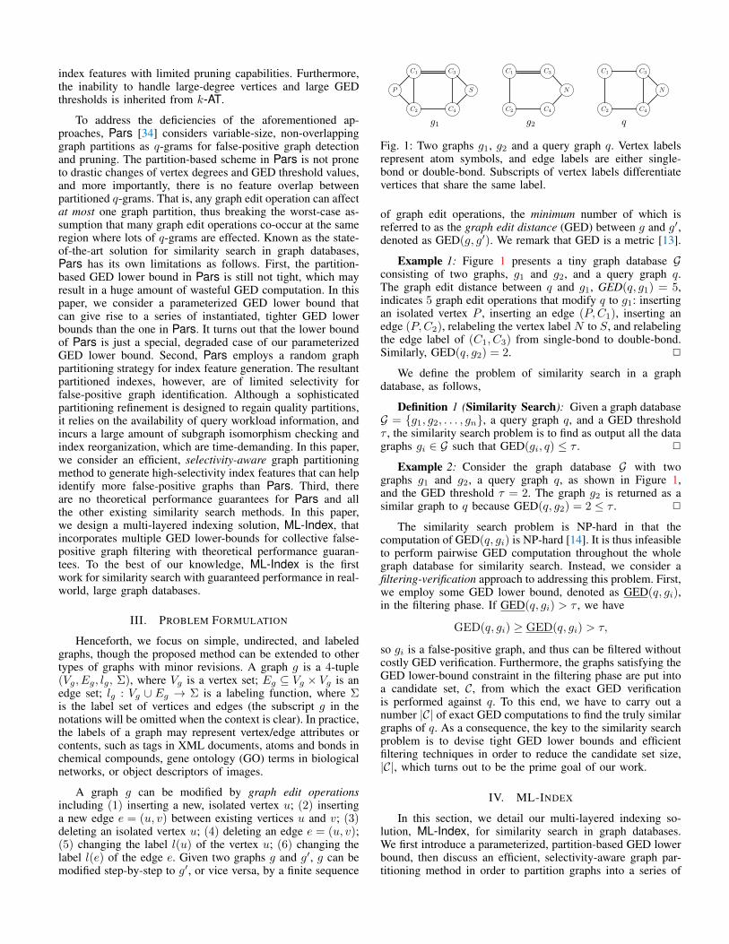
Fig. 2: The graph g1 in Figure 1 is partitioned into four half-edge graphs: P(g1) = {p1, p2, p3, p4}.

high-selectivity subgraph partitions, which comprise the mainindex features of ML-Index for the evaluation of GED lowerbounds. Finally, we design and implement ML-Index, uponwhich multiple partition-based GED lower bounds can beevaluated synergistically for false-positive graph identificationand filtering with theoretical performance guarantees.

A. Partition-based GED Lower Bounds

We first define half-edge graphs [34] that model andrepresent graph partitions and also index features of ML-Index.

Definition 2 (Half-edge Graph): A half-edge graph g =(Vg, Eg, lg,Σ), where Eg ⊆ Vg × (Vg ∪ {∗}), is a graphwith possible existences of half edges (u, ∗) ∈ Eg , whereone incident vertex u ∈ Vg is a definite vertex, but the othervertex (and its label) of the half edge is not explicitly specified,represented as ∗. 2

Definition 3 (Half-edge Subgraph Isomorphism):A half-edge graph g is a subgraph of another graph g′,denoted as g ⊆ g′, if there exists an injective subgraphisomorphism function f : Vg → Vg′ , such that (1)∀u ∈ Vg, f(u) ∈ Vg′ and lg(u) = lg′(f(u)); (2) ∀(u, v) ∈Eg, (f(u), f(v)) ∈ Eg′ and lg((u, v)) = lg′((f(u), f(v)));(3) ∀(u, ∗) ∈ Eg,∃w ∈ Vg′\f(Vg) s.t. (f(u), w) ∈ Eg′ andlg((u, ∗)) = lg′((f(u), w)). 2

If g ⊆ g′, g is a half-edge subgraph of g′, or a subgraph of g′for brevity. Intuitively, if g ⊆ g′, we say g is contained in g′, org′ contains g. We remark that half-edge subgraph isomorphismis NP-complete in that ordinary graphs without the specialvertex ∗ can be regarded as a special case of half-edge graphs,and the subgraph isomorphism problem for ordinary graphshas proven to be NP-complete [14].

Definition 4 (Graph Partitioning): A graph g can bepartitioned to a set P of collective exhaustive, mutuallyexclusive, and non-empty half-edge graphs as P(g) ={pi|

⋃i Vpi = Vg,

⋃iEpi ⊆ Eg ∪ Vg × {∗}, pi

⋂pj =

∅, ∀i, j, i 6= j}. P is called a partitioning of g. 2

Example 3: As shown in Figure 2, the graph g1 in Fig-ure 1 is partitioned into four half-edge graphs, p1, p2, p3, andp4. So P = {p1, p2, p3, p4} is one partitioning, among others,of g1. 2

Partitioning graphs into half-edge subgraphs has a clearadvantage for GED estimation: given any graph edit operation,it can only affect at most one half-edge graph partition. Asa result, we derive the following partition-based GED lowerbound:

Theorem 1: Consider a graph g that is partitioned to a setP(g) of (τ+k) half-edge graphs, where τ is the GED thresholdand k (k ≥ 1) is an integer parameter. Given the query graphq, if GED(g, q) ≤ τ , there must exist at least k partitions ofg, pi1 , . . . , pik ∈ P(g), that satisfy pil ⊆ q (1 ≤ l ≤ k). 2

Proof: Please refer to Appendix A.

Consider a data graph g ∈ G and a partitioning P(g) ={p1, . . . , pτ+k}. If pi ⊆ q, pi is called a matching partition.Otherwise, pi is a mismatching partition. According to The-orem 1, if the number of matching partitions of g w.r.t. q isless than k, the graph edit distance, GED(g, q), must be largerthan τ . Therefore, g is a false-positive graph and can be safelypruned without exact GED verification.

Example 4: Consider the graph database G = {g1, g2}and the query graph q as shown in Figure 1, and the GEDthreshold τ = 2. We set k = 2 such that g1 and g2 are par-titioned into (τ + k) = 4 partitions, respectively. Specifically,the partitioning of g1, P(g1), is shown in Figure 2. Becausethere exist three mismatching partitions w.r.t. q: p1, p2, andp4, g1 is thus a false-positive graph. However, no matter whatgraph partitioning methods applied on g2, we can always findat least k = 2 matching partitions. Therefore, g2 is a candidategraph that further needs exact GED verification. 2

Theorem 1 provides a parameterized, partition-based GEDlower bound that can immediately generate a series of newGED lower bounds by setting k with different values. Weremark that 1 ≤ k ≤ ming∈G(|Vg| − τ), and the newlygenerated GED lower bounds have varied filtering capabilities.When k = 1, the instantiated GED lower bound boils down toa special, degraded case [34]. Consider a graph g ∈ G whichis a false positive w.r.t. the query graph q. It is easy to find one(k = 1) matching partition given the (τ + 1) partitions of g.Once found, g will be treated as a candidate graph by mistake.When k > 1, however, g as a false-positive graph will morelikely be identified and filtered, as detecting k > 1 matchingpartitions from g becomes less likely than in the case of k = 1.This is demonstrated in the following theorem,

Theorem 2: Consider a false-positive graph g ∈ G(GED(q, g) > τ ) that is partitioned to P = {p1, . . . , pτ+1}and P ′ = {p′1, . . . , p′τ+k}, k > 1, respectively. If we assumegraph edit operations occur irrespective of g, the probability ofthe first k partitions of P ′ being matching partitions is smallerthan the probability of the first one partition of P being amatching partition. 2

Proof: Please refer to Appendix A.

If we partition graphs of G into (τ + k) partitions, wherek > 1, it is more likely to identify false-positive graphs fromG than the degraded case of k = 1. As a consequence, thegeneralized GED lower bound can be instantiated into a seriesof tigher lower bounds, when k > 1, with better filteringcapabilities for similarity search.

B. Selectivity-aware Graph Partitioning

Given a data graph g ∈ G, there exist a huge number ofways to partition g into (τ+k) partitions with varied sizes andstructures [6]. If not designed carefully, a partitioning method(e.g., random partitioning) may lead to graph partitions withlimited filtering capabilities. Therefore, graph partitioning alsoplays a critical role in evaluating partitioned-based GED lowerbounds for similarity search in graph databases.

Example 5: For the same problem setting as describedin Example 4, if g1 in Figure 1 is partitioned by a random

P

C1

C2

C3

C4

S P

C1

C2 C4

C3

S

p′1

p′2

p′3

p′4

Fig. 3: The graph g1 in Figure 1 is randomly partitioned intofour half-edge graphs, P ′(g) = {p′1, p′2, p′3, p′4}, with limitedselectivity.

partitioning method, P ′, into four half-edge graphs, p′1, p′2,p′3, and p′4, as shown in Figure 3, we note that both p′2 and p′3are matching partitions w.r.t. q, because p′2 ⊆ q and p′3 ⊆ q.Based on Theorem 1 (k = 2), g1 is a candidate graph, althoughit is in fact a false-positive graph and should be filtered if thepartitioning method P in Example 3 is employed. 2

In order to devise partitioning algorithms that lead topartitions with good filtering capabilities, we define the notionof selectivity for half-edge graph partitions. Consider anypartitioning scheme P that partitions a graph g into (τ + k)partitions, P = {p1, . . . , pτ+k}. We design a selectivityfunction s : pi ∈ P → R+ assigning for each partitionpi(1 ≤ i ≤ τ + k) a positive value, s(pi), indicating howselective pi will be as a mismatching partition (pi * q) ifg is a false-positive graph. Intuitively, the higher the valueof s(pi) is, the more probably pi is a mismatching partition,and the false-positive graph g will more easily be identifiedand filtered from G. To this end, the objective of a selectivity-aware partitioning P is to partition a graph g into (τ + k)partitions, which have the highest overall selectivity values.However, even for the simplest, balanced bi-partitioning case(P = {p1, p2}), the number of possible partitionings is(

|Vg||Vg|/2

)=

|Vg|!((|Vg|/2)!)2

≈ 2|Vg|√

2/(π|Vg|),

and finding the optimal selectivity-aware partitioning is NP-hard, which is polynomially reducible from the l-way graphpartitioning problem [5], [14].

In the following, we design an efficient selectivity-awaregraph partitioning method. We first model the selectivity ofgraph partitions based on the following heuristics:

1) Partition size: a larger-size partition pi is more likelyto be affected by graph edit operations, thus makingpi a mismatching partition. We thus consider thegraph size, (|Vpi | + |Epi |), as one aspect of theselectivity;

2) Vertex/Edge label frequency: vertices/edges of piwith small label frequencies in G may occur propor-tionally rarely in the query q. Therefore, a partitionpi containing low-frequency vertices/edges might bea mismatching partition, pi q. We thus considerthe average vertex/edge label frequencies as anotheraspect related to the selectivity of pi.

To incorporate both factors, we define the selectivity, s(pi), ofa partition pi as

s(pi) =|Vpi |+ |Epi |∑

v∈Vpif(lv)/|Vpi |+

∑e∈Epi

f(le)/|Epi |(1)

where f(·) is the vertex/edge label frequency in G. If thereexists a half-edge (v, ∗) in pi, its edge label frequency is

Algorithm 1: Selectivity-aware Graph PartitioningInput: a graph g ∈ G, GED threshold τ , parameter kOutput: The partitioning P(g) = {p1, . . . , pτ+k}

1 begin2 A Boolean vector B[·] : Vg → {true, false} where

∀v ∈ Vg, B[v]← false;3 Γ← ∅;4 for i← 1 to τ + k do5 Select v ∈ Vg where B(v) = false, pi ← {v};6 B(v)← true;7 for u ∈ N(v), B[u] = false, u 6∈ Γ do8 Γ← Γ ∪ {u};

9 while ∃v ∈ Γ do10 for i← 1 to τ + k do11 ∆i ← s(G[pi ∪ {v}])− s(pi);12 pi∗ ← G[pi∗ ∪ {v}] where i∗ = arg maxi ∆i;13 B(v)← true;14 for u ∈ N(v), B[u] = false, u 6∈ Γ do15 Γ← Γ ∪ {u};

16 while ∃(u, v) ∈ Eg, u ∈ pi, v ∈ pj , i 6= j do17 ∆i ← s(pi ∪ (u, ∗))− s(pi);18 ∆j ← s(pj ∪ (v, ∗))− s(pj);19 if ∆i ≥ ∆j then20 pi ← pi ∪ {(u, ∗)};21 else22 pj ← pj ∪ {(v, ∗)};

23 return P(g) = {p1, . . . , pτ+k};

estimated as

f(l(v,∗)) =

∑u∈N (v) f(l(v,u))

|N (v)|(2)

where N (v) is the set of neighboring vertices of v in G.

The selectivity-aware partitioning algorithm is presentedin Algorithm 1, which partitions a graph g ∈ G into (τ + k)partitions (half-edge graphs). We first create a Boolean vectorB[·] indicating for each vertex v ∈ Vg whether v has beenassigned to some partition, and B[v] is initialized to false(Line 2). We maintain another set, Γ, holding the unassignedvertices of g that will be processed immediately (Line 3). Next,we choose (τ + k) vertices as the initial seeds, which will beexpanded to the final (τ + k) partitions (Lines 4 − 6). Theneighboring vertices, N(·), of these seeds are added to Γ asthey will be considered for partition assignment in the next step(Lines 7− 8). Henceforth, we examine each vertex v ∈ Γ byevaluating the selectivity gain of assigning v to each existingpartition pi, denoted as

∆i = s(G[pi ∪ {v}])− s(pi), 1 ≤ i ≤ τ + k (3)

where G[pi ∪ {v}] denotes the induced subgraph if v andall its induced edges (u, v), u ∈ Vpi are inserted to thepartition pi (Lines 10 − 11). The vertex v will be assignedto the partition pi∗ which, with the addition of v (and itsinduced edges), has the largest selectivity gain, ∆i∗ (Line 12).After v has been assigned to some partition, all its unassignedneighboring vertices are added to Γ for further inspection

(Lines 14 − 15). When all vertices of g have been properlyassigned to the (τ + k) partitions, we then consider the edgesstraddling different partitions and assign them as half-edges toone of the participant partitions. The principle of assignmentis similar: for the edge (u, v) where u ∈ Vpi , v ∈ Vpj , i 6= j,we assign it to the partition that leads to a larger selectivitygain (Lines 16− 22).

We remark that the vertex/edge label frequencies can bepre-computed by scanning the graph database G once duringthe index construction phase. Therefore, the time complexity ofAlgorithm 1 is O((τ+k)|Vg|+|Eg|), or simply O(|Vg|+|Eg|)considering (τ + k) is a small value in similarity search.

C. The Multi-layered Index Structure

In order to filter false positive graphs from the graphdatabase G, we build an index structure upon which partition-based GED lower bounds can be evaluated in an efficient andcost-effective way. For each data graph g ∈ G, we partition itinto (τ + k) half-edge subgraphs, which constitute the basicindex features. In addition, for each partition p, we maintainthe following crucial information:

1) Inverted index: If p is a partition of the graph gi ∈ G,we maintain for p an inverted index, I(p), containingthe graph identifier i as p ⊆ gi. Given a query graphq, if p ⊆ q, we can quickly locate all the graphs fromI(p), each of which has p as a matching partition.Furthermore, by exploring all the indexed partitions,we can find graphs of G that contain at least kmatching partitions, which constitute the candidateset C for exact GED verification;

2) Graph profile: A common operation we have toperform frequently is to examine if p ⊆ q holds as amatching partition, or p * q as a mismatching pat-tern otherwise. This half-edge subgraph isomorphismtesting is time-consuming in practice. We thereforeconstruct a graph profile, R(p), for the partition pto facilitate this computation. R(p) maintains thevertex/edge label frequencies of p in a space-efficienthistogram. Before examining p ⊆ q, their graph pro-files, R(p) and R(q), are first compared bucket-wise:For each vertex/edge label in R(p), its frequencyshould be no more than that of the correspondingvertex/edge label in R(q), denoted as R(p) � R(q).Otherwise, we immediately know that p * q, and thecostly half-edge subgraph isomorphism computationcan be saved.

It is possible two partitions are graph isomorphic with eachother. We thus use the canonical DFS code [29] as a uniquerepresentation of graph partitions to ensure that two isomorphicpartitions will share one index entry represented by theircanonical DFS code.

The aforementioned index structure is a conventional, one-layer graph index designed for similarity search. However,it promises limited filtering capabilities due to the followingreasons. First, only a single GED lower bound is adoptedfor false-positive graph filtering. Although we can choose atight, partition-based GED lower bound (when k > 1) andtake advantage of high-selectivity index features generatedby the selectivity-aware graph partitioning method, there are

Algorithm 2: ML-Index ConstructionInput: Graph database GOutput: The multi-layer index ML-Index

1 begin2 for i← 1 to L do3 A hash structure, Hi : p→ (I(p),R(p)), is

initialized as ∅;4 foreach g ∈ G do5 for i← 1 to L do6 Pi(g) = {pi1, . . . , piτ+ki};7 for l← 1 to τ + ki do

/* Inverted index */8 I(pil)← I(pil) ∪ {g};

/* Graph profile */9 R(pil)← a histogram of vertex/edge

label frequencies for pil;10 Hi(pil) = (I(pil),R(pil));

11 return ML-Index {H1, . . . ,HL};

still many false-positive graphs unidentified from the graphdatabase G. Second, and more importantly, there are no the-oretical tightness guarantees for GED lower bounds, whichtypically lead to unstable, and sometimes poor, similaritysearch performance in real-world graph databases.

In order to take advantage of multiple GED lower boundsand exert a collective filtering strategy, we design a multi-layered graph indexing structure, ML-Index, to enhance fil-tering capabilities with theoretical performance guarantees. InML-Index, we consider L different graph partitioning methods,P1, . . . ,PL, with each Pi partitioning g ∈ G into (τ +ki) par-titions, Pi(g) = {pi1, . . . , piτ+ki}. To this end, the partitioningmethod Pi, the instantiated GED lower bound (parameterizedby ki), and the resultant graph partitions (together with theirassociated inverted indexes and graph profiles) constitute theith layer of ML-Index. Namely, ML-Index consists of L layersof indexes, with each layer being responsible for the evaluationof the ith GED lower-bound. Given a query graph q, weexamine ML-Index layer-by-layer. Specifically, at the ith layer,we evaluate the ith GED lower bound parameterized by ki, andgenerate a candidate set Ci. A data graph g ∈ G is a candidategraph at the ith layer if and only if there exist at least kimatching partitions from g:

Ci = {g|∃ pil1 . . . , pilki⊆ g and q, g ∈ G} (4)

where pil∗ are the partitioned index features at the ith layer ofML-Index. As a result, the final candidate set C after all LGED lower bounds of ML-Index have been evaluated is

C =

L⋂i=1

Ci (5)

Given a graph g ∈ G, if it fails in the evaluation of a GEDlower-bound at any layer of ML-Index, it must be a false-positive graph, and can be safely filtered without exact GEDverification.

Algorithm 2 presents the index construction process forML-Index with L layers of partition-based indexes. Each layerof ML-Index is a hash structure,Hi(1 ≤ i ≤ L), that maintains

p11

......Layer 1

......

C

C C

O

I( )Inverted index

O C C

C

C

C

C

O

Graph profile

( , )k1P1

......

......

......Layer L( , )kLPL

......

......p1i

p21

p22

pL1

pLj

p1i

R( )p1i

g3

g5

Layer 2( , )k2P2

Fig. 4: The multi-layered index structure of ML-Index. Eachlayer i is featured a partitioning strategy Pi, the partitionedindex features {pi1, pi2, . . . , }, and an instantiated GED lowerbound parameterized by ki. Each index feature pij is associatedwith an inverted index I(pij) and a graph profile R(pij).

the correlation between a partition p and the associated invertedindex, I(p), and its graph profile, R(p) (Lines 2−3). We startwith a sequential scan of the graph database G, and for eachdata graph g ∈ G, we partition it using L different partitioningmethods1. Each partitioning Pi yields (τ +ki) partitions fromg, which constitute the index features at the ith layer of ML-Index (Lines 4−6). For each partition pil (1 ≤ l ≤ τ+ki), wefurther maintain its inverted index (Line 8) and its graph profile(Line 9), and associate them with pil in the hash structure Hi(Line 10). We remark that different partitioning methods mayresult in identical graph partitions (in terms of half-edge graphisomorphism) at different layers of ML-Index, we maintainonly one copy of the inverted index and the graph profileto save the index space. Figure 4 illustrates the schematicstructure of ML-Index.

The time complexity of Algorithm 2 is O(|G|×L×(O(P)+O(|Vg|+ |Eg|))), where O(P) is the average-time complexityof graph partitioning, and O(|Vg|+|Eg|) is the time complexityof graph profile construction for all partitions of g ∈ G. If theselectivity-aware graph partitioning (Section IV-B) is adopted,the time complexity of Algorithm 2 turns out to be O(|G| ×L × (|V | + |E|)), where (|V | + |E|) is the average size ofgraphs in G. The space complexity of ML-Index is O(L ×|F| × (|G|+ |Σ|)), where |F| is the average number of indexpartitions at each layer of ML-Index, and Σ is the label set ofvertices and edges of G.

Theorem 3: Consider a graph g ∈ G, which is a falsepositive w.r.t. the query graph q, i.e., GED(q, g) > τ . The prob-ability of g being identified as a false positive by ML-Indexgets exponentially large (approaching 1) w.r.t. the number Lof independent GED lower bounds in ML-Index. 2

Proof: Please refer to Appendix A.

Theorem 3 states that ML-Index is guaranteed to identifyfalse-positive graphs from G w.h.p. by crosschecking multipleindependent GED lower bounds. In order to secure the inde-pendency of the partition-based GED lower bounds in ML-Index, we consider the following strategies in index construc-tion. First, we randomly select initial seeds from g ∈ G whenapplying the selectivity-aware partitioning method at differentlayers of ML-Index. Second, we choose different values of theparameter ki at different layer i of ML-Index. This way, the

1Note that we can apply the same selectivity-aware partitioning algorithmwith different initial seeds (by random selection), and different values of theparameter ki, thus resulting in L different sets of partitioned index features.

Algorithm 3: Similarity Search AlgorithmInput: Graph database G, query graph q, GED

threshold τ , ML-Index {H1, . . . ,HL}Output: O = {g|GED(g, q) ≤ τ, g ∈ G}

1 begin/* Candidate Generation */

2 Create an array A that maintains for each graphg ∈ G the number of matching partitions w.r.t. q;

3 for i← 1 to L do4 foreach g ∈ G do5 A[g]← 0;6 for p ∈ Hi do7 if R(p) � R(q) and (p ⊆ q) then8 foreach g ∈ I(p) do9 A[g]← A[g] + 1;

10 Ci ← ∅;11 foreach g ∈ G do12 if A[g] ≥ ki then13 Ci ← Ci ∪ {g};

14 C ←⋂Li=1 Ci;

/* GED Verification */15 O ← ∅;16 foreach g ∈ C do17 if GED(g, q) ≤ τ then18 O ← O ∪ {g};

19 return The result set O;

index partitions and the GED lower-bound constraints will varysignificantly across different layers of ML-Index. As a result,ML-Index has the theoretical tightness guarantee for the GEDlower bound, which was not promised in the existing, state-of-the-art similarity search solutions.

We also remark that ML-Index is a generalized graphindexing framework. The GED lower bounds in ML-Index arenot confined to partitioned-based lower bounds, so any existingGED lower bound can be synergistically incorporated in ML-Index to enable a powerful, collective filtering strategy towardsbringing a significant false-positive reduction for similaritysearch with theoretical performance guarantees.

V. SIMILARITY SEARCH ALGORITHM

After ML-Index is built from G, we can use it to answersimilarity search queries, as detailed in Algorithm 3. We firstcreate an array A[·] to maintain for each data graph g ∈ G,the number of matching partitions w.r.t. the query q (Line 2),and it is initialized to 0 (Lines 4− 5). At the ith layer of ML-Index (1 ≤ i ≤ L), we evaluate for each partitioned indexfeature p if p ⊆ q is satisfied (the graph profile checking,R(p) � R(q), is performed first to short-circuit the costlyhalf-edge subgraph isomorphism testing, p ⊆ q). If p ⊆ q istrue, p is a matching partition w.r.t. q, and it is also a half-edge subgraph of all the data graphs g ∈ G in p’s invertedindex, I(p). We thus increment A[g], accordingly (Lines 6−9).Based on Theorem 1, the candidate set at the ith layer of ML-Index, Ci, includes all the data graphs with no less than kimatching partitions, where ki is the instantiated GED lower-

bound parameter at the ith layer of ML-Index (Lines 10−13).After this layer-by-layer evaluation, the final candidate set, C,contains the data graphs satisfying all L disparate GED lower-bounds specified in ML-Index (Line 14). Finally, we adoptsome exact GED computational method to achieve the finalresults, O, from C (Lines 15− 19).

To examine the time complexity of Algorithm 3, we con-sider the following critical factors: (1) Tiso : the average timecomplexity of half-edge subgraph isomorphism from indexfeature p to the query q, p ⊆ q; (2) Tged : the averagetime complexity of exact GED computation, GED(q, g), whereg ∈ G; and (3) To : all the other time consumed forinitialization and set-based operations. As a result, the overallruntime cost of Algorithm 3 can be formulated as

T = |L⋃i=1

Hi| ∗ Tiso + |L⋂i=1

Ci| ∗ Tged + To. (6)

Specifically, the first component, |⋃Li=1Hi| ∗ Tiso, represents

the overall time to generate the candidate sets at different layersof ML-Index, while the second component, |

⋂Li=1 Ci| ∗ Tged,

is the overall time for GED verification. Former empiricalstudies have demonstrated that Tiso is typically three orders ofmagnitude less than Tged in real-world graphs [34]. Therefore,the main computational bottleneck lies in the GED verificationcomponent, |

⋂Li=1 Ci| ∗ Tged, and the key to enhancing simi-

larity search performance is to reduce the candidate set size,|C| = |

⋂Li=1 Ci|, which is also the goal of ML-Index. We

also note that by introducing the multi-layered index structurefor ML-Index, we have to spend extra space for new indexfeatures and extra time for half-edge subgraph isomorphismtestings. However, the significant gain in false-positive graphreductions has far outweighed such marginal cost, as reportedin Section VI.

VI. EXPERIMENTS

A. Graph Databases

We consider three publicly available graph databases tobenchmark different similarity search methods. The details ofgraph databases are summarized as follows,

1) AIDS: this is an antivirus screen chemical com-pound database from the Developmental Therapeu-tics Program at NCI/NIH2. There are 42, 687 graph-structured chemical compounds with 25.6 verticesand 27.6 edges by average, and 62 vertex labels (likeelements C, O, N, and P) and 3 edge labels in total;

2) PROTEIN: this is a protein graph database from theProtein Data Bank3 containing 600 graphs with 32.6vertices and 62.1 edges by average. There are 3 vertexlabels and 5 edge labels in this database. The graphsare denser and less label-informative than those in theAIDS database;

3) GRAPHGEN: this is a synthetic graph generatorthat creates large collections of labeled graphs4. Thegenerator is regulated by a series of parameters: the

2dtp.nci.hih.gov/docs/aids/aids data.html3www.iam.unibe.ch/fki/databases/iam-graph-database4www.cse.ust.hk/graphgen

number of graphs, |G|, the average size of each graphin terms of the number of edges, |E|, the numberof unique vertex/edge labels, |Σ|, and the averagedensity of graphs, defined as d = 2|E|/|V |(|V | − 1).If not specified explicitly otherwise, the default pa-rameters are set as: |G| = 10K, |E| = 40, d = 0.1,|Σ| = 4/4 denoting there are 4 distinct vertex labelsand 4 distinct edge labels, respectively.

The query set Q is generated by randomly sampling 100graphs from each graph database, respectively. That is, querygraphs in Q have similar structure/label characteristics as thedata graphs in the corresponding graph databases.

B. Experimental Setup

We carry out experimental studies for ML-Index in com-parison with Pars [34], which has outperformed other existingsimilarity search methods [37], [28], [35], [27], and been byfar the most efficient algorithm. In particular, we consider thefollowing algorithms in the experimental studies,

1) Pars[34]: the state-of-the-art graph indexing methodadopting a single, degraded GED lower bound (k =1) and random partitioning for index generation andsimilarity search;

2) Selectivity: a single-layer graph indexing methodusing the generalized GED lower bound with aninstantiated parameter k > 1 (Theorem 1), and theselectivity-aware graph partitioning (Algorithm 1) forindex generation and similarity search;

3) ML-Index-L: a multi-layered graph indexing methodcomprising L distinct layers, each of which representsa distinct partition-based GED lower bound param-eterized by ki, and a selectivity-aware partitioningmethod, Pi, for index generation. We set L = 4 inreal-world graph databases, and L = 3 in syntheticgraph databases (When L is set with other values, wehave witnessed similar experimental findings, whichare omitted for brevity).

We consider the following performance evaluation metricsin the experimental studies: (1) Index construction cost,including the number |F| of partitioned index features, thein-memory index size M , and the index construction time T ;(2) Candidate set size, |C|, which is the most critical indicatorof the similarity search performance. The results reported hereare the average candidate set size for 100 queries in the queryset Q; (3) Query execution time, consisting of the time forcandidate generation and the time for exact GED verification,is the real response time for similarity search. Again, thetime reported here is the average response time of 100 givenqueries in Q. In our experiments, we use the state-of-the-artmethod [22] for exact GED verification.

All our experiments were carried out on an Intel i73.20GHz quad-core PC with 8GB memory running Windows7 operating system. The algorithms are implemented in C++and compiled in Microsoft Visual Studio 2015.

C. Experiments for Index Construction

First of all, we evaluate the index construction cost ofdifferent methods in different graph databases. Note that all

50K

100K

150K

200K

250K

1 2 3 4 5 6

Num

ber

of I

ndex

Fea

ture

s |F

|

GED Threshold τ

ParsSelectivity

ML-Index-2ML-Index-3

ML-Index-4

(a) |F| vs. τ (AIDS)

10

20

30

40

50

60

70

80

90

100

1 2 3 4 5 6

Inde

x Si

ze (

MB

ytes

)

GED Threshold τ

ParsSelectivity

ML-Index-2ML-Index-3

ML-Index-4

(b) M vs. τ (AIDS)

500

1000

1500

2000

2500

3000

1 2 3 4 5 6

Inde

x C

onst

ruct

ion

Tim

e (S

ec.)

GED Threshold τ

ParsSelectivity

ML-Index-2ML-Index-3ML-Index-4

(c) T vs. τ (AIDS)

0K

5K

10K

15K

20K

1 2 3 4 5 6

Num

ber

of I

ndex

Fea

ture

s |F

|

GED Threshold τ

ParsSelectivity

ML-Index-2

ML-Index-3ML-Index-4

(d) |F| vs. τ (PROTEIN)

0.5

1

1.5

2

1 2 3 4 5 6

Inde

x Si

ze (

MB

ytes

)

GED Threshold τ

ParsSelectivity

ML-Index-2

ML-Index-3ML-Index-4

(e) M vs. τ (PROTEIN)

0

0.5

1

1.5

2

1 2 3 4 5 6

Inde

x C

onst

ruct

ion

Tim

e (S

ec.)

GED Threshold τ

ParsSelectivity

ML-Index-2ML-Index-3ML-Index-4

(f) T vs. τ (PROTEIN)

0K

100K

200K

300K

400K

500K

600K

700K

800K

10K 20K 40K 60K 80K

Num

ber

of I

ndex

Fea

ture

s |F

|

Graph Database Size

ParsSelectivity

ML-Index-2ML-Index-3

(g) |F| vs. |G|

0

20

40

60

80

100

120

10K 20K 40K 60K 80K

Inde

x Si

ze (

MB

ytes

)

Graph Database Size

ParsSelectivity

ML-Index-2ML-Index-3

(h) M vs. |G|

0

10

20

30

40

50

60

70

80

90

10K 20K 40K 60K 80K

Inde

x C

onst

ruct

ion

Tim

e (S

ec.)

Graph Database Size

ParsSelectivity

ML-Index-2ML-Index-3

(i) T vs. |G|

40K

60K

80K

100K

120K

140K

160K

0.1 0.2 0.3 0.4 0.5

Inde

x Pa

rtiti

on N

umbe

r |F

|

Graph Density

ParsSelectivity

ML-Index-2ML-Index-3

(j) |F| vs. d

4

6

8

10

12

14

16

18

20

0.1 0.2 0.3 0.4 0.5

Inde

x Si

ze (

MB

ytes

)

Graph Density

ParsSelectivity

ML-Index-2ML-Index-3

(k) M vs. d

5

10

15

20

0.1 0.2 0.3 0.4 0.5

Inde

x C

onst

ruct

ion

Tim

e (S

ec.)

Graph Density

ParsSelectivity

ML-Index-2ML-Index-3

(l) T vs. d

50K

100K

150K

200K

250K

4/4 6/6 8/8 10/10

Inde

x Pa

rtiti

on N

umbe

r |F

|

Graph Labels |Σ|

ParsSelectivity

ML-Index-2ML-Index-3

(m) |F| vs. |Σ|

5

10

15

20

25

4/4 6/6 8/8 10/10

Inde

x Si

ze (

MB

ytes

)

Graph Labels |Σ|

ParsSelectivity

ML-Index-2ML-Index-3

(n) M vs. |Σ|

2

4

6

8

10

12

4/4 6/6 8/8 10/10

Inde

x C

onst

ruct

ion

Tim

e (S

ec.)

Graph Labels |Σ|

ParsSelectivity

ML-Index-2ML-Index-3

(o) T vs. |Σ|Fig. 5: Index construction cost in terms of the number of index features, |F|, the index size M (in megabytes), and the indexconstruction time T (in seconds) for different similarity search methods in different graph databases.

graph indexes are pre-built offline, given a graph database, G,and we consider the GED threshold, τ , with practically smallvalues (τ ≤ 6), as users are typically more inclined to searchfor similar graphs from graph databases.

We first examine the index construction cost in the AIDSgraph database. The number |F| of index features, the indexsize M , and the index construction time T of different methodsare illustrated in Figure 5(a), (b), and (c), respectively. InFigure 5(a), by varying the values of τ from 1 up to 6,we recognize that the numbers of index features, |F|, ofthe one-layer indexing methods, Pars and Selectivity, arefairly stable and close with each other, while |F| of themulti-layered indexing approaches, ML-Index-2, ML-Index-3, and ML-Index-4, decrease steadily. This is because agrowing number of selectivity-aware partitions in the multi-layered indexes turn out to be identical (in terms of half-edgesubgraph isomorphism), and their inverted indexes and graphprofiles can be reused across different layers of ML-Index, thusresulting in succinct index structures. This is further verifiedin terms of the index size, M (in megabytes), as shown inFigure 5(b). Even for the largest index, ML-Index-4, withfour layers of partitioned index features, it only consumesless than 80 megabytes, which is very cost-effective, andcan safely reside in memory. As to the index constructiontime T (in seconds) in Figure 5(c), we find that the multi-layered index ML-Index can be built efficiently. In particular,the index construction time T for multi-layered indexes isslightly greater than the construction time for single-layerindexing methods (T for ML-Index-4 is within 2.5x of T forSelectivity, given different values of τ ). With the increase ofτ , this gap of index construction time becomes marginal. Thisis mainly because when τ gets larger, each data graph g ∈ G isaccordingly partitioned into a larger number (τ+k) of smaller-

size partitions, thus leading to a speedup in half-edge subgraphisomorphism computation, which typcailly takes more than90% of the total index construction time.

We then examine the index construction cost in the PRO-TEIN graph database, the graphs of which are dense and withfew vertex/edge labels. The experimental results are illustratedin Figure 5(d)-(f). Here we witness similar trends and findingsas the ones from the AIDS database, with one exception thatthere are much fewer numbers of identical index partitionsshared by different layers of ML-Index, thus leading to asteady growth of the number of index features, |F|, w.r.t. τ , asshown in Figure 5(d). However, the memory M consumedby different graph indexes is still very small (less than 2megabytes even for ML-Index-4), as shown in Figure 5(e), andall indexes can be successfully constructed within 2 seconds,as shown in Figure 5(f).

We further evaluate the index construction cost on a seriesof synthetic graph databases generated by GRAPHGEN, andset τ = 5 by default in the following experiments. Figure 5(g)-(i) present the scalability results of index construction fordifferent methods. By varying the number of data graphs, |G|,from 10K up to 80K, we recognize that the number of indexfeatures, |F|, the index size M , and the index constructiontime T all grow linearly, exhibiting excellent scalability forall different graph indexing methods. For the largest graphdatabase with 80K graphs, the size of ML-Index-3 is 131megabytes, and it can be efficiently built within 90 seconds.

We then tune the graph density parameter, d, to gen-erate graph databases with varied graph densities, and theexperimental results for index construction are illustrated inFigure 5(j)-(l). When d increases from 0.1 to 0.5, the numberof index features, |F|, decreases steadily for Selectivity, ML-

0K

5K

10K

15K

20K

25K

30K

35K

40K

45K

1 2 3 4 5 6

Can

dida

te S

et S

ize

|C|

GED Threshold τ

ParsSelectivity

ML-Index-2ML-Index-3ML-Index-4

Real

(a) |C| vs. τ (AIDS)

0

50

100

150

200

250

1 2 3 4 5 6

Can

dida

te S

et S

ize

|C|

GED Threshold τ

ParsSelectivity

ML-Index-2ML-Index-3ML-Index-4

Real

(b) |C| vs. τ (PROTEIN)

0K

10K

20K

30K

40K

50K

10K 20K 40K 60K 80K

Can

dida

te S

et S

ize

|C|

Graph Database Size |G|

ParsSelectivity

ML-Index-2ML-Index-3

Real

(c) |C| vs. |G|

0K

2K

4K

6K

8K

10K

12K

0.1 0.2 0.3 0.4 0.5

Can

dida

te S

et S

ize

|C|

Graph Density

ParsSelectivity

ML-Index-2

ML-Index-3Real

(d) |C| vs. d

0K

1K

2K

3K

4K

5K

6K

7K

8K

9K

4/4 6/6 8/8 10/10

Can

dida

te S

et S

ize

|C|

Graph Labels |Σ|

ParsSelectivity

ML-Index-2ML-Index-3

Real

(e) |C| vs. |Σ|

100

101

102

103

104

105

1 2 3 4 5 6

Run

time

(sec

.)

GED Threshold τ

Pars

Selectivity

ML-Index-2

ML-Index-3

ML-Index-4

Can. Gen.

(f) Runtime (AIDS)

10-2

10-1

100

101

102

1 2 3 4 5 6

Run

time

(sec

.)

GED Threshold τ

Pars

Selectivity

ML-Index-2

ML-Index-3

ML-Index-4

Can. Gen.

(g) Runtime (PROTEIN)

10-1

100

101

102

103

104

10K 20K 40K 60K 80K

Run

time

(sec

.)

Graph Database Size |G|

Pars

Selectivity

ML-Index-2

ML-Index-3

Can. Gen.

(h) Runtime vs. |G|

100

101

102

103

104

0.1 0.2 0.3 0.4 0.5

Run

time

(sec

.)

Graph Density d

Pars

Selectivity

ML-Index-2

ML-Index-3

Can. Gen.

(i) Runtime vs. d

10-1

100

101

102

103

104

4/4 6/6 8/8 10/10

Run

time

(sec

.)

Graph Labels |Σ|

Pars

Selectivity

ML-Index-2

ML-Index-3

Can. Gen.

(j) Runtime vs. |Σ|Fig. 6: The similarity search performance in terms of the candidate set size, |C|, and the overall runtime, T .

Index-2, and ML-Index-3, because a growing number ofselectivity-aware partitions turn out to be identical, whichare graph partitions shared by dense graphs in the graphdatabase. As a result, the index size M decreases steadily aswell. However, the index construction time T increases as ittypically takes more time to partition denser graphs.

Finally, we examine the index construction cost w.r.t. thelabel set size, |Σ|. We generate a series of graph databases witha varied number of vertex/edge labels, and construct graphindexes in these graph databases. The experimental results arepresented in Figure 5(m)-(o). We note that when there are moredistinct vertex/edge labels in the graph database, both |F| andM grows slightly larger, due primarily to a more diverse setof index features generated from the graph database. However,the index construction time T is very stable for all differentgraph indexing methods.

D. Experiments for Similarity Search

We then report our experimental studies for the similaritysearch performance of different methods in different graphdatabases. We consider the candidate set size, |C|, as the prin-cipal indicator for similarity search performance. Furthermore,we also report the overall runtime concerning both candidategeneration and exact GED verification, which is also the realresponse time for similarity search in graph databases.

Figure 6(a) illustrates the candidate set size, |C|, w.r.t.the GED threshold, τ , for different methods in the AIDSdatabase. We also include the size, |O|, of the similarity searchresults to demonstrate the ultimate goal we strive to attain(colored in pink triangles). We have the following importantfindings in the experimental studies. First of all, the valuesof |C| for Selectivity (colored in red circle) are consistentlysmaller than those for Pars (colored in green square), withan average reduction of 30% false-positive graphs in thecandidate set. The reason is two-fold. First, the generalizedGED lower bound with parameter k > 1 is tighter than thedegraded one (k = 1). Second, the selectivity-aware parti-tioning method in Selectivity is more effective than randompartitioning in Pars toward generating high-selectivity indexpartitions, which further help filter false-positive graphs duringcandidate generation. More importantly, we recognize that

the multi-layered indexing approaches, including ML-Index-2, ML-Index-3, and ML-Index-4, have achieved significantfalse-positive graph reductions during candidate generation.With the increase of the number L of layers in ML-Index, wefind |C| is guaranteed to reduce consistently, indicating thatthe multi-layered indexing method, ML-Index, has excellentfiltering capabilities, and can bring guaranteed improvementfor false-positive graph reduction in comparison to the single-layer graph indexing methods such as Pars and Selectivity.In particular, ML-Index-4 is the most effective method whosecandidate sets, C, are 2.5x to 10.7x smaller than the onesreturned by the state-of-the-art method, Pars.

The same experiments are carried out in the PROTEINdatabase, and the results are presented in Figure 6(b). It canbe witnessed that, given different values of τ , the multi-layered indexing methods, ML-Index-2, ML-Index-3, and ML-Index-4, achieve significant and consistent false-positive graphreductions, compared with the single-layer indexing methods.Specifically, the candidate sets, C, of ML-Index-4 are 3.4xup to 17.6x smaller than the ones returned by Pars, leadingto significant performance gains for similarity search givendifferent values of τ .

We further evaluate the candidate set sizes, |C|, in a seriesof synthetic graph databases. First of all, we examine thescalability results for similarity search by varying the numberof graphs ranging from 10K up to 80K in the graph databaseG, and report the candidate set sizes, |C|, for different methods,as shown in Figure 6(c). We note that, with a growth of thenumber of graphs in G, the number of candidate graphs, |C|,returned by Pars increases significantly, which will incur alarge amount of costly GED computation. However, when weintroduce the multi-layered index structure in ML-Index, asignificant portion of false-positive graphs are identified andfiltered even in very large graph databases. In particular, ML-Index-4 achieves at least an order of magnitude improvementfor false-positive graph reductions, compared with Pars, ingraph databases of different sizes.

We then generate a series of graph databases (|G| = 10K)with varied graph densities d ranging from 0.1 up to 0.5,and examine the similarity search performance in these graphdatabases. The experimental results are reported in Figure 6(d).We recognize that when graphs become dense, the numbers

|C| of candidate graphs returned by different similarity searchmethods turn out to increase significantly. The reason is that,given a dense graph g ∈ G, some of its (τ+k) graph partitionsbecome dense accordingly. As a result, the probability ofmore than one graph edit operations arising from a densepartition, pi, increases as well. However, once identified as amismatching partition, pi is only counted as one mismatchingpartition in the GED lower bound evaluation, though theremight be multiple graph edit operations co-occur within pi.This phenomenon indicates that the detection of false positivegraphs becomes difficult for dense graphs. However, even inthis hard case, ML-Index-4 still outperforms Pars, meaningthat it is beneficial to crosscheck multiple GED lower boundsto ensure effective false-positive reductions especially in thegraph databases with many dense graphs.

We also examine how the number of vertex/edge labels,|Σ|, of a graph database is related to |C|, and the results arepresented in Figure 6(e). When |Σ| increases, a significantreduction of |C| has been recognized for all different methods.Interestingly enough, when |Σ| = 6/6 (and larger), ML-Index-2 and ML-Index-3 can successfully identify and filter all false-positive graphs from C. Namely, C = O. This indicates that theconsideration of vertex/edge labels in the modeling and designof the selectivity-aware graph partitioning method turns out tobe effective, which leads to high-selectivity index partitionsfrom graph databases, and results in significant reductions offalse-positive graphs during similarity search.

We finally evaluate the overall runtime cost of all similaritysearch methods in different graph databases, and the results areillustrated in Figure 6(f)-(j) (Note that the experimental settingsare the same as in the corresponding experimental studies for|C|, respectively). The similarity search response time reportedhere comprise both the time for candidate generation (coloredin grey), and the time for exact GED verification. We note thatthe time spent for candidate generation is at most several sec-onds, which is marginal in comparison with the time spent forexact GED verification. In the two real-world graph databases,AIDS (Figure 6(f)) and PROTEIN (Figure 6(g)), the multi-layered indexing method, ML-Index-4, achieves an order ofmagnitude improvement in the similarity search performance,compared with the state-of-the-art method, Pars, especiallywhen the GED threshold, τ , is small (τ ≤ 3). Meanwhile, in aseries of synthetic graph databases characterized by the graphdatabase size |G| (Figure 6(h)), graph density d (Figure 6(i)),and the number of vertex/edge labels |Σ| (Figure 6(j)), thesearch performance gap between ML-Index-3 and Pars canbe as large as two orders of magnitude. This further verifiesthat our multi-layered graph indexing approach, ML-Index, isan efficient and high-performance similarity search methodin real-world and synthetic graph databases under differentexperimental settings.

VII. CONCLUSION

The similarity search problem plays a fundamental andcritical role in managing and querying graph-structured data,and has found widely varying applications in real-world large-scale graph databases. In this paper, we considered the simi-larity search problem that is defined on the graph edit distance(GED) constraint, and further proposed a new, multi-layeredgraph indexing solution, ML-Index, to address this challenging

problem in graph databases. We employed a parameterized,partition-based GED lower bound for false-positive graphidentification and filtering, and designed a selectivity-awaregraph partitioning algorithm for high-quality index featuregeneration. We further incorporated and crosschecked multipleinstantiated GED lower bounds in ML-Index such that false-positive graphs can be filtered with theoretical performanceguarantees. The experimental studies on both real and syn-thetic graph databases have demonstrated that ML-Index isan efficient and cost-effective indexing method, which hassignificantly outperformed the state-of-the-art method, Pars,for similarity search in large-scale graph databases.

REFERENCES

[1] C. C. Aggarwal and H. Wang. Managing and Mining Graph Data.Springer Inc., 2010.

[2] P. Barcelo Baeza. Querying graph databases. In Proceedings of the32nd Symposium on Principles of Database Systems (PODS’13), pages175–188, 2013.

[3] H. M. Berman, J. Westbrook, Z. Feng, G. Gilliland, T. N. Bhat,H. Weissig, I. N. Shindyalov, and P. E. Bourne. The protein data bank.Nucleic Acids Res, 28:235–242, 2000.

[4] S. Berretti, A. Del Bimbo, and E. Vicario. Efficient matching andindexing of graph models in content-based retrieval. IEEE Trans.Pattern Anal. Mach. Intell., 23(10):1089–1105, 2001.

[5] C.-E. Bichot and P. Siarry. Graph Partitioning. Wiley, 2011.

[6] A. Buluc, H. Meyerhenke, I. Safro, P. Sanders, and C. Schulz. Recentadvances in graph partitioning. ArXiv e-prints, 2013.

[7] H. Bunke. On a relation between graph edit distance and maximumcommon subgraph. Pattern Recogn. Lett., 18(9):689–694, 1997.

[8] H. Bunke. Error correcting graph matching: On the influence of theunderlying cost function. IEEE Trans. Pattern Anal. Mach. Intell.,21(9):917–922, 1999.

[9] H. Bunke and K. Shearer. A graph distance metric based on the maximalcommon subgraph. Pattern Recogn. Lett., 19(3-4):255–259, 1998.

[10] D. Conte, P. Foggia, C. Sansone, and M. Vento. Thirty years ofgraph matching in pattern recognition. International Journal of PatternRecognition and Artificial Intelligence, 18(3):265–298, 2004.

[11] D. J. Cook and L. B. Holder. Mining Graph Data. John Wiley & Sons,2006.

[12] S. Fankhauser, K. Riesen, and H. Bunke. Speeding up graph editdistance computation through fast bipartite matching. In Proceedingsof the 8th International Conference on Graph-based Representations inPattern Recognition (GBRPR’11), pages 102–111, 2011.

[13] X. Gao, B. Xiao, D. Tao, and X. Li. A survey of graph edit distance.Pattern Anal. Appl., 13(1):113–129, 2010.

[14] M. R. Garey and D. S. Johnson. Computers and Intractability; A Guideto the Theory of NP-Completeness. W. H. Freeman & Co., New York,NY, USA, 1990.

[15] K. Gouda and M. Arafa. An improved global lower bound for graphedit similarity search. Pattern Recogn. Lett., 58:8–14, 2015.

[16] H. He and A. K. Singh. Graphs-at-a-time: query language and accessmethods for graph databases. In Proceedings of the 2008 ACM SIGMODinternational conference on Management of data (SIGMOD’08), pages405–418, 2008.

[17] H. W. Kuhn and B. Yaw. The hungarian method for the assignmentproblem. Naval Res. Logist. Quart, pages 83–97, 1955.

[18] L. Libkin, W. Martens, and D. Vrgoc. Querying graphs with data. J.ACM, 63(2):14:1–14:53, 2016.

[19] M. Neuhaus and H. Bunke. Bridging the Gap Between Graph EditDistance and Kernel Machines. World Scientific Publishing, 2007.

[20] H. Ogata, S. Goto, K. Sato, W. Fujibuchi, H. Bono, and M. Kanehisa.KEGG: kyoto encyclopedia of genes and genomes. Nucleic AcidsResearch, 27(1):29–34, 1999.

[21] S. Ranu, M. Hoang, and A. Singh. Answering top-k representativequeries on graph databases. In Proceedings of the 2014 ACM SIGMODInternational Conference on Management of Data (SIGMOD’14), pages1163–1174, 2014.

[22] K. Riesen, S. Emmenegger, and H. Bunke. A novel software toolkitfor graph edit distance computation. In 9th International Workshop onGraph-Based Representations in Pattern Recognition, pages 142–151,2013.

[23] H. Shang, X. Lin, Y. Zhang, J. X. Yu, and W. Wang. Connected sub-structure similarity search. In Proceedings of the 2010 ACM SIGMODInternational Conference on Management of Data (SIGMOD’10), pages903–914, 2010.

[24] Z. Sun, H. Wang, H. Wang, B. Shao, and J. Li. Efficient subgraphmatching on billion node graphs. Proc. VLDB Endow., 5(9):788–799,2012.

[25] Y. Tian, R. C. Mceachin, C. Santos, D. J. States, and J. M. Patel.SAGA: A subgraph matching tool for biological graphs. Bioinformatics,23(2):232–239, 2007.

[26] E. Ukkonen. Approximate string-matching with q-grams and maximalmatches. Theor. Comput. Sci., 92(1):191–211, 1992.

[27] G. Wang, B. Wang, X. Yang, and G. Yu. Efficiently indexing largesparse graphs for similarity search. IEEE Trans. on Knowl. and DataEng., 24(3):440–451, 2012.

[28] X. Wang, X. Ding, A. K. H. Tung, S. Ying, and H. Jin. An efficientgraph indexing method. In Proceedings of the 2012 IEEE 28thInternational Conference on Data Engineering (ICDE’12), pages 210–221, 2012.

[29] X. Yan and J. Han. gSpan: Graph-based substructure pattern mining.In Proceedings of the 2002 IEEE International Conference on DataMining (ICDM’02), pages 721–724, 2002.

[30] X. Yan, P. S. Yu, and J. Han. Substructure similarity search in graphdatabases. In Proceedings of the 2005 ACM SIGMOD InternationalConference on Management of Data (SIGMOD’05), pages 766–777,2005.

[31] Y. Yuan, G. Wang, J. Y. Xu, and L. Chen. Efficient distributed subgraphsimilarity matching. The VLDB Journal, 24(3):369–394, 2015.

[32] Z. Zeng, A. K. H. Tung, J. Wang, J. Feng, and L. Zhou. Comparingstars: On approximating graph edit distance. Proc. VLDB Endow.,2(1):25–36, 2009.

[33] S. Zhang, J. Yang, and W. Jin. SAPPER: Subgraph indexing andapproximate matching in large graphs. Proc. VLDB Endow., 3(1-2):1185–1194, 2010.

[34] X. Zhao, C. Xiao, X. Lin, Q. Liu, and W. Zhang. A partition-basedapproach to structure similarity search. PVLDB, 7(3):169–180, 2013.

[35] X. Zhao, C. Xiao, X. Lin, and W. Wang. Efficient graph similarityjoins with edit distance constraints. In Proceedings of the 2012 IEEE28th International Conference on Data Engineering (ICDE’12), pages834–845, 2012.

[36] X. Zhao, C. Xiao, X. Lin, W. Wang, and Y. Ishikawa. Efficientprocessing of graph similarity queries with edit distance constraints.The VLDB Journal, 22(6):727–752, 2013.

[37] W. Zheng, L. Zou, X. Lian, D. Wang, and D. Zhao. Graph similaritysearch with edit distance constraint in large graph databases. InProceedings of the 22nd ACM International Conference on Conferenceon Information & Knowledge Management (CIKM’13), pages 1595–1600, 2013.

[38] G. Zhu, X. Lin, K. Zhu, W. Zhang, and J. X. Yu. TreeSpan:Efficiently computing similarity all-matching. In Proceedings of the2012 ACM SIGMOD International Conference on Management of Data(SIGMOD’12), pages 529–540, 2012.

[39] Y. Zhu, L. Qin, J. X. Yu, and H. Cheng. Finding top-k similar graphs ingraph databases. In Proceedings of the 15th International Conferenceon Extending Database Technology (EDBT’12), pages 456–467, 2012.

APPENDIX

Proof of Theorem 1. We assume, by contradiction, that thereare less than k partitions of g that are half-edge subgraphisomorphic to q. Namely, there are more than (τ +k)−k = τ

partitions that are not half-edge subgraph isomorphic to q. Foreach pi of these τ partitions where pi ( q, we need at leastone graph edit operation to modify pi in order to modify g toq as a consequence, thus amounting up to more than τ graphedit operations, which is in contradiction to the known factthat GED(g, q) ≤ τ . 2

Proof of Theorem 2. Based on the assumption that all graphedit operations occur irrespectively of g, we cast the GEDproblem into the classic balls-and-bins model, where graphedit operations correspond to m = GED(q, g) balls, and (τ+k)partitions correspond to n = τ + k bins. Such m balls will beplaced into n bins, and a matching partition pi ⊆ q (1 ≤ i ≤τ + k) corresponds to an empty bin because there is no graphedit operation occurring in pi. Since any ball is placed intoa bin with an equal probability of 1/n, the probability of thefirst bin out of (τ + 1) bins being empty is

(1− 1

n)m = (

τ

τ + 1)GED(q,g)

while the probability of the first k bins out of (τ + k) binsbeing empty is

(1− k

n)m = (

τ

τ + k)GED(q,g)

Because GED(q, g) > τ ≥ 0, we remark that when k > 1

(τ

τ + k)GED(q,g) < (

τ

τ + 1)GED(q,g)

2

Proof of Theorem 3. Given the false-positive graph g, wedenote the probability of g being detected as a false positiveby the i-th GED lower bound at the i-th layer (1 ≤ i ≤ L) ofML-Index is Pri(g). So, the probability of g that fails to bedetected and filtered at the i-th layer of ML-Index is 1−Pri(g).Analogously, the probability of g satisfying all L GED lower-bounds at L different layers of ML-Index while still not beingdetected as a false positive is

∏Li=1(1 − Pri(g)). Therefore,

the probability of g being identified as a false positive by ML-Index is

1−L∏i=1

(1− Pri(g)). (7)

Assume that ML-Index adopts the naive random partition-ing method at all L different layers for graph partitioning andindex generation, and we further assume Pri(g) = 1/2 forall 1 ≤ i ≤ L. That is, the probability of whether g can besuccessfully identified as a false-positive graph, or not, at anylayer of ML-Index is half-half. (Noth that the values of GEDlower-bound parameters, ki, can be different, thus resulting indifferent index partitions with varied filtering capabilities atdifferent layers of ML-Index, and if we choose the selectivity-aware graph partitioning method, as opposed to the randompartitioning, the probability Pri(g) can be significantly higher).Then, the probability of g being identified as a false positivegraph by ML-Index is

1−L∏i=1

(1− 1

2) = 1− 1

2L,

which can be exponentially high and approaches 1, when thenumber L of index layers of ML-Index is set large. 2