Sim ultaneous Measurement - Reed College · Sim ultaneous Measurement of ... b y Arth urs and Kelly...

Simultaneous Measurement

of

Noncommuting Quantum Observables

Nicholas Wheeler

October 2012

Introduction. In 1965, E. Arthurs and J. L. Kelly, Jr.—who were employedas engineers at Bell Lab—published in BSTJ Briefs a short paper1 bearinga title “On the simultaneous measurement of conjugate observables” whichmost quantum physicists could be expected to find perplexing. Within a fewmonths C. Y. She and H. He!ner devised an alternative approach2 to thetheory of simultaneous measurement that reproduced the results first obtainedby Arthurs and Kelly, and by about 1980 the subject—stimulated mainly bythe practical needs of quantum opticians and the development of quantuminformation theory—had begun to generate wide interest.3

That early work took John von Neumann’s idealized theory of quantummeasurement as its point of departure, but more recently the theory ofgeneralized (non-ideal) quantum measurement has been brought into play. Itis from that point of view that S. M. Barnett approaches the subject,4 andit is Barnett’s brief survey (intended to illustrate the utility of the positiveoperator-valued measure (POVM) concept) that has motivated the followingdiscussion.

1 Bell Systems Technical Journal 44, 725–729 (1965). This was a journalseldom consulted by most physicists (it ceased publication in 1983), though itwas the journal in which the results of the Davisson-Germer electron di!ractionexperiment were first reported (1928), the journal in which Claude Shannonpublished his “A mathematical theory of communication” (1948), the journalin which W. Boyle and G. E. Smith announced their invention of the charge-coupled device (1970) and in which many other important developments werefirst reported.

2 “Simultaneous measurement of noncommuting observables,”Phys.Rev.152,1103–1110 (1966).

3 For major references see the bibiography in Ingrid Olson, “Simultaneousmeasurement of conjugate observables” (Reed College Thesis, 2006).

4 Quantum Information (2009), pages 97–98.

2 Simultaneous measurement of noncommuting observables

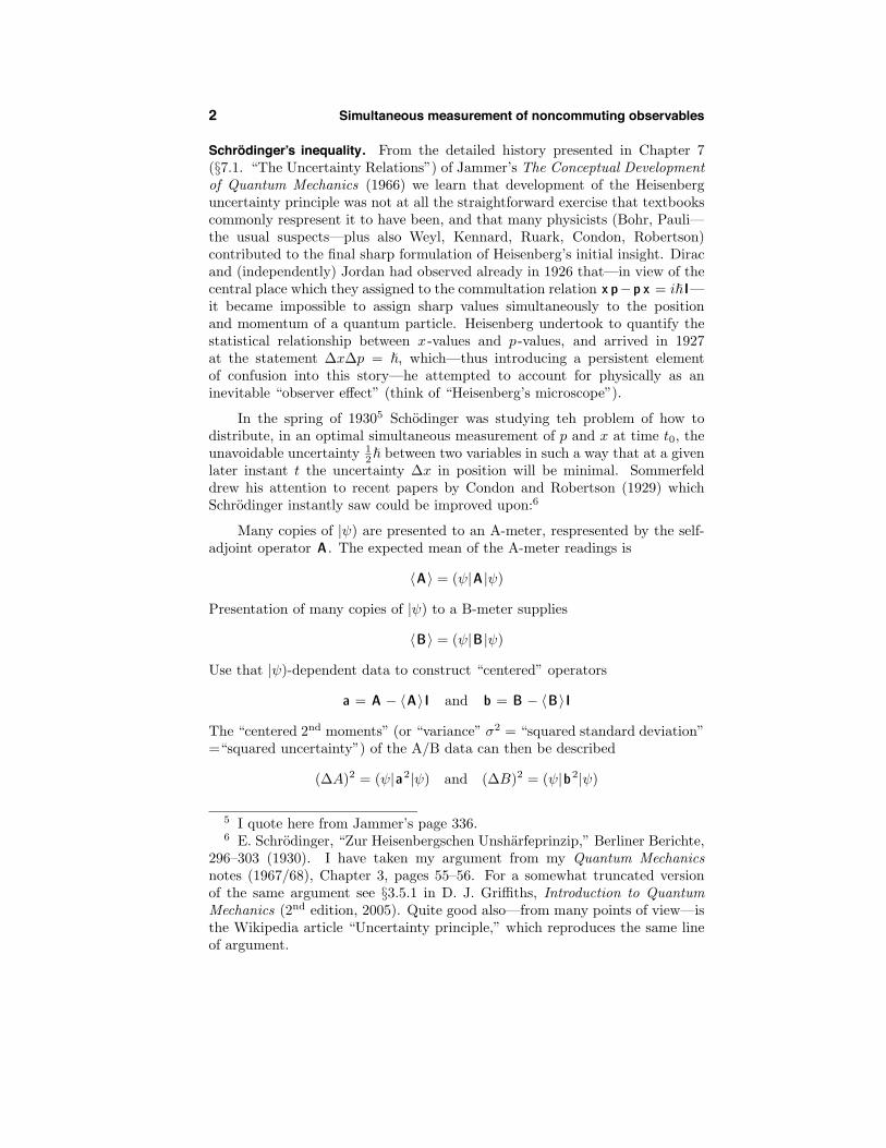
Schrodinger’s inequality. From the detailed history presented in Chapter 7(§7.1. “The Uncertainty Relations”) of Jammer’s The Conceptual Developmentof Quantum Mechanics (1966) we learn that development of the Heisenberguncertainty principle was not at all the straightforward exercise that textbookscommonly respresent it to have been, and that many physicists (Bohr, Pauli—the usual suspects—plus also Weyl, Kennard, Ruark, Condon, Robertson)contributed to the final sharp formulation of Heisenberg’s initial insight. Diracand (independently) Jordan had observed already in 1926 that—in view of thecentral place which they assigned to the commultation relation x p! p x = i! I—it became impossible to assign sharp values simultaneously to the positionand momentum of a quantum particle. Heisenberg undertook to quantify thestatistical relationship between x-values and p -values, and arrived in 1927at the statement "x"p = !, which—thus introducing a persistent elementof confusion into this story—he attempted to account for physically as aninevitable “observer e!ect” (think of “Heisenberg’s microscope”).

In the spring of 19305 Schodinger was studying teh problem of how todistribute, in an optimal simultaneous measurement of p and x at time t0, theunavoidable uncertainty 1

2! between two variables in such a way that at a givenlater instant t the uncertainty "x in position will be minimal. Sommerfelddrew his attention to recent papers by Condon and Robertson (1929) whichSchrodinger instantly saw could be improved upon:6

Many copies of |!) are presented to an A-meter, respresented by the self-adjoint operator A . The expected mean of the A-meter readings is

"A# = (!|A |!)

Presentation of many copies of |!) to a B-meter supplies

"B# = (!|B |!)

Use that |!)-dependent data to construct “centered” operators

a = A ! "A# I and b = B ! "B# I

The “centered 2nd moments” (or “variance” "2 = “squared standard deviation”=“squared uncertainty”) of the A/B data can then be described

("A)2 = (!|a2|!) and ("B)2 = (!|b2|!)

5 I quote here from Jammer’s page 336.6 E. Schrodinger, “Zur Heisenbergschen Unsharfeprinzip,” Berliner Berichte,

296–303 (1930). I have taken my argument from my Quantum Mechanicsnotes (1967/68), Chapter 3, pages 55–56. For a somewhat truncated versionof the same argument see §3.5.1 in D. J. Gri#ths, Introduction to QuantumMechanics (2nd edition, 2005). Quite good also—from many points of view—isthe Wikipedia article “Uncertainty principle,” which reproduces the same lineof argument.

Schrodinger’s inequality 3

Define|a) = a |!) and |b) = b |!)

Then by the Cauchy-Schwarz

("A)2("B)2 = (a|a)(b|b)$ (a|b)(b|a) = |(a|b)|2 with equality i! |a) % |b)

= |(!|a b |!)|2

Writea b = a b + b a

2+ i a b ! b a

2i

and notice that the self-aqjointness of a and b implies that of both 12 [a , b ]+

and 12i [a , b ]!. We therefore have

("A)2("B)2 $!!!"

a b + b a2

#+ i

"a b ! b a

2i

#!!!2

="

a b + b a2

#2+

"a b ! b a

2i

#2

By quick calculation

a b ± b a =$

A B + B A ! 2A"B# ! 2B"A# + 2"A#"B#A B ! B A

so"a b ± b a# =

$"A B + B A# ! 2"A#"B#"A B ! B A#

which gives Schrodinger’s inequality

("A)2("B)2 $"

A B ! B A2i

#2+

%"A B + B A

2

#! "A#"B#

&2(1.1)

$ greater of$"

A B ! B A2i

#2,

%"A B + B A

2

#! "A#"B#

&2'

(1.2)

In the most familiar instance we therefore have

("x)2("p)2 $"

x p ! p x2i

#2+

%"x p + p x

2

#! "x#"p#

&2

$"

x p ! p x2i

#2=

"i! I2i

#2= (!/2)2

&"x"p $ 1

2!

In classical statistics, if x and y are random variables then one has (for allm and n)

"xmyn# = "xm#"yn# i! x ane y are statistically independent

The number "xy # ! "x#"y # provides therefore a leading indicator of the extentto which x and y are statistically dependent or correlated. On the right side


of (1) we encounter just such a construction

CAB [|!)] '"

a b + b a2

#=

"A B + B A

2

#! "A#"B# (2)

which it becomes natural in this light to call the “quantum correlationcoe#cient.”7

If A and B commute then (1.2) supplies

("A)2("B)2 $("A B# ! "A#"B#

)2

The eigenvectors (but not the eigenvalues) of A and B are in this case shared.If |!) is such a shared eigenvector (A |!) = #|!) and B |!) = $|!)) then

("A)2("B)2 $ [#$ ! #$ ]2 = 0= 0 because "A = "B = 0

But linear combinations of such (orthogonal) eigenvectors give "A "B > 0.Suppose, for example, that |!) = cos % |!1) + sin % |!2). Then

CAB [|!)] = (#1$1 cos2 % + #2$2 sin2 %)

! (#1 cos2 % + #2 sin2 %)($1 cos2 % + $2 sin2 %)

= (#1 ! #2)($1 ! $2) cos2 % sin2 %

which give back the preceding result as a degenerate special case (set % = n&/2with n = 0,±1,±2, . . .).

More interesting are results that follow from the assumption that A and Bare conjugate:

A B ! B A = i I

Introduce operators

W = 1"2(A + iB) and W+ = 1"

2(A ! iB)

which—since not self-adjoint—do not represent observables, but are the key toall that follows. From

W W+ = 12 (A A ! iA B + iB A + B B) = 1

2 (A A + B B + I)W+W = 1

2 (A A + iA B ! iB A + B B) = 12 (A A + B B ! I)

obtainW W+ ! W+W = I =(

$W W+ = W+W + IW+W = W W+ ! I

7 See page 202 inD. Bohm,Quantum Mechanics (1951). Generally A B )= B A .In (2) we are told to “split the di!erence.”


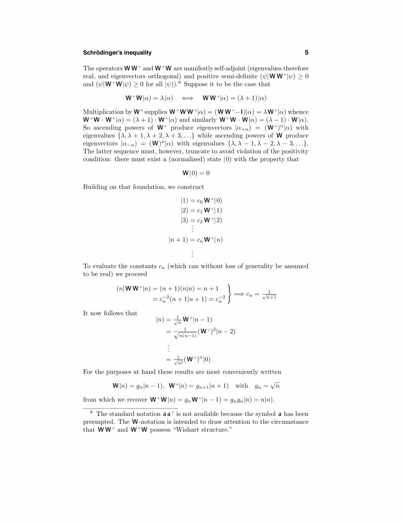
The operators W W+ and W+W are manifestly self-adjoint (eigenvalues thereforereal, and eigenvectors orthogonal) and positive semi-definite (!|W W+|!) $ 0and (!|W+W |!) $ 0 for all |!)).8 Suppose it to be the case that

W+W |#) = ' |#) *( W W+|#) = (' + 1) |#)

Multiplication by W+ supplies W+W W+|#) = (W W+! I)|#) = 'W+|#) whenceW+W · W+|#) = (' + 1) · W+|#) and similarly W+W · W |#) = (' ! 1) · W |#).So ascending powers of W+ produce eigenvectors |#+n) = (W+)n|#) witheigenvalues {', ' + 1, ' + 2, ' + 3, . . .} while ascending powers of W produceeigenvectors |#!n) = (W)n|#) with eigenvalues {', ' ! 1, ' ! 2, ' ! 3, . . .}.The latter sequence must, however, truncate to avoid violation of the positivitycondition: there must exist a (normalized) state |0) with the property that

W |0) = 0

Building on that foundation, we construct

|1) = c0 W+|0)|2) = c1 W+|1)|3) = c2 W+|2)

...|n + 1) = cn W+|n)

...

To evaluate the constants cn (which can without loss of generality be assumedto be real) we proceed

(n|W W+|n) = (n + 1)(n|n) = n + 1

= c!2n (n + 1|n + 1) = c!2

n

*=( cn = 1"

n+1

It now follows that|n) = 1"

nW+|n ! 1)

= 1+n(n!1)

(W+)2|n ! 2)

...= 1"

n!(W+)n|0)

For the purposes at hand these results are most conveniently written

W |n) = gn|n ! 1), W+|n) = gn+1|n + 1) with gn =+

n

from which we recover W+W |n) = gn W+|n ! 1) = gngn|n) = n|n).

8 The standard notation a a+ is not available because the symbol a has beenpreempted. The W -notation is intended to draw attention to the circumstancethat W W+ and W+W possess “Wishart structure.”


Variants of the preceding algebra are encountered in many quantummechanical contexts, all of which derive from Dirac’s approach to the harmonicoscillator problem.9 It is central to quantum optics (quantized oscillatorymodes of the radiation field),10 And it provides the formal model upon whichWitten’s “supersymmetric quantum mechanics” is based.11 But the immediatepoint of the exercise emeerges when we look back again to Schrodinger’sinequality (1). If the state presented repeatedly to the A-meter on Monday—and to the B-meter on Tuesday—is |n), and if A and B are conjugate([A , B ] = i I) then

("A)2("B)2 $ 14 +

+CAB [|n)]

,2

whereCAB [|n)] = 1

2 (n|A B + B A |n) ! (n|A |n)(n|B |n)

But fromA = 1"

2(W+ + W) and B = i 1"

2(W+ ! W)

we obtainA B + B A = i(W+W+ ! W W)

so12

CAB [|n)] = i 12

-(n|W+W+ ! W W |n) ! (n|W+ + W |n)(n|W+ ! W |n)

.

= i 12

-gn+1gn+2(n|n + 2) ! gn!1gn(n|n ! 2)

!(gn+1(n|n + 1) + gn(n|n ! 1)

)(gn+1(n|n + 1) ! gn(n|n ! 1)

).

= 0 by (n|m) = (nm (3)

For such states we therefore have

(n|A |n) = (n|B |n) = 0 and "A"B $ 12

The inequality can, however, be sharpened; from

(n|A2|n) = (n|B2|n) = 12 (n|W+W + W W+|n) + two terms that vanish

= 12

(gngn + gn+1gn+1

)(n|n)

= 12 (2n + 1)

9 §34, Principles of Quantum Mechanics (3rd edition, 1947). For an accountof some elegant elaborations of the method due to Schwinger see Chapter 0,pages 40–42 in my Advanced Quantum Topics (2000).

10 See, for example, §3.1.1 in Yoshihisa Yamamoto & Atac Imamoglu,Mesoscopic Quantum Optics (1999).

11 See Christopher Lee, “Supersymmetric quantum mechanics” (Reed CollegeThesis, 1999), which provides an elaborate bibliography.

12 If n = 0 or 1 some of the terms in the following expression—namely g!1,|!1) and |!2)—are undefined, but those formal artifacts all vanish, essentiallybecause Wp|0) = 0 : p = 1, 2, . . . .


we obtain"A"B = n + 1

2 $ 12

It is no accident that those numbers are proportional to the energy eigenvaluesEn = !)(n + 1

2 ) of a quantum oscillator.

The states |n) acquire importance partly (as in oscillator theory) from thecircumstance that they are eigenstates of W+W and W W+, but more generallyfrom (3); they are minimal uncertainty states that in quantum mechanicsengender wavepackets of “minimal dispersion”(see Gri#ths6, §3.5.2) and inquantum optics13 are called “coherent states.”

The simplest possible non-commutation relation [A , B ] = i I (from whichthe preceding discussion proceeded) does not admit of finite-dimensionalrealization (compare the traces of the left and right sides of [A, B ] = i I).But finite-dimensional quantum mechanics presents many contexts in whichSchrodinger’s inequality proves valuable. Most commonly those arise when onehas in hand either a trace-wise orthonormal basis {E1, E2, . . . , EN2} in the spaceof N , N hermitian matrices

A =N

2/

j=1

ajEj with ak = 1N

trAEk by 1N

trEjEk = (jk

or a set {F1, F2, . . . , Fn} of hermitian matrices that is closed under commutation(in short, a Lie algebra):

[Fi, Fj ] =/

k

cik

jFk

Look, for example, to the Pauli matrices

""0 =0

1 00 1

1, ""1 =

00 11 0

1, ""2 =

00 !ii 0

1, ""3 =

01 00 !1

1

which possess both of the aforementioned properties: they are trace-wiseorthonormal

12 tr ""m""n = (mn

and since multiplicatively closed

""0""n = ""n : n = 0, 1, 2, 3""j""k = (jk""0 + i*jkl""l : {j, k, l} = 1, 2, 3

are closed also under commutation: [""j , ""k ] = 2i*jkl""l. Suppose

A = a1""1 + a2""2 + a3""3 = aaa···"" and B = bbb···""

13 See C. C. Gerry & P. L. Knight, Introductory Quantum Optics (2005),Chapter 3.


Then AB = (aaa···bbb)""0 + i(aaa , bbb)···"" supplies

AA = (aaa···aaa)""0 and BB = (bbb···bbb)""0

AB + BA = 2(aaa···bbb)""0

AB ! BA = 2i(aaa , bbb)···""

and we have "A# =2

ak"""k# = "aaa···""# and "B# = "bbb···""# whence

("A)2("B)2 =((aaa···aaa) ! "aaa···""#2

)((bbb···bbb) ! "bbb···""#2

)(4.1)

while the Schrodinger inequality supplies a statement with quite a di!erentappearance:

("A)2("B)2 $3(aaa , bbb)···""

42 +((aaa···bbb) ! "aaa···""#"bbb···""#

)2 (4.2)

Butwhen(withMathematica’s assistance) I usedrandomlyselected real 3-vectorsaaa and bbb to construct hermitian matrices A and B I was surprised to find thatfor every the normalized complex 2-vector |!) the expressions on the right sidesof (4.1) and (4.2) are identical ; we have stumbled upon a curious identity

(aaa···aaa)(bbb···bbb) ! (aaa···bbb)2 = (bbb···bbb)"aaa···""#2 + (aaa···aaa)"bbb···""#2 +3(aaa , bbb)···""

42

! 2(aaa···bbb)"aaa···""#"bbb···""# (5.1)

In the case A = ""1, B = ""2 the preceding identity assumes the (strange but)suggestively simple form

1 = (!|""1|!)2 + (!|""2|!)2 + (!|""3|!)2 : all |!) (5.2)

I am satisfied on the basis of exhaustive numerical evidence that the identities(5) are both correct, which means that the $ in (4.2) should always be readas equality. . . for, as it happens, a very simple reason. The $ in question wasinherited from Cauchy-Schwarz, and reduces to = if and only if

|#) ' A|!) ! (!|A|!) · |!) % |$ ) ' B|!) ! (!|B|!) · |!)

From (!|#) = (!|$) = 0 we learn that both of those vectors are orthogonalto |!), which in 2-space means that they are proportional: |#) % |$ ). We arebrought thus to the striking conclusion that when a randomly selected qubit |!)is presented repeatedly first to an arbitrarily designed A-meter and then—ina separate run—to an arbitrarily designed B-meter, analysis of the data thusgenerated invariably shows the product "A"B to be minimal.14 In higher-dimensional contexts automatic minimality is lost, for a reason now evident.

14 When we wrote A = aaa···"" and B = bbb···"" we tacitly assumed the matricesA and B to be traceless, but it is now clear that invariable minimality persistseven in the absence of tracelessness.

What does Schrodinger’s inequality signify? 9

Suppose the states presented to our meters are not identical, but are drawnfrom the mixed ensemble described by the density operator !. Review of itsderivation shows that Schrodinger’s inequality (1) remains in force, provided

"XXX# = (!|XXX|!) is reinterpreted to mean tr(!XXX)

Note in this regard that the e!ect state superposition |!) !- c1|!1) + c2|!2)—which sends pure states to pure states—is non-linear

(!|XXX|!) - c1c1(!1|XXX|!1) + c1c2(!1|XXX|!2) + c2c1(!2|XXX|!1) + c2c2(!2|XXX|!2)

while the e!ect of mixing ! !- p1!1 + p2!2 is linear

tr(!XXX) !- p1tr(!1XXX) + p2tr(!2XXX)

Non-linear e!ects do, however, enter into the description of CAB [p1!1 + p2!2]via the "A#"B# term; “mixtures of minimal states”15 are not minimal.

What does Schrodinger’s inequality signify? Present copies of |!) (else statesdrawn from the mixed ensemble !) many times to an A-meter and from themeter readings {a1, a2, . . . , amany} compute the emperical mean a and thecentered moments

(a ! a)p : p = 2, 3, 4, . . .

of which "A# and3(A ! "A#)p

4= (!|

5A ! (!|A |!)

6p|!) else tr5!(A ! tr!A)p

6

by the Born Rule provide theoretical estimates. Do the same—in a separateexperimental run—with a B-meter. The Schrodinger inequality (1) describes aninevitable relationship among the lowest-order moments {"Ap#, "Bp#} : p = 1, 2,the statement of which requires however that one have access also to data

"C#, "D# with C = 12i (A B ! B A), D = 1

2 (A B + B A)

acquired from two additional experiments.

There is, of course, no end to the list {A , B , C , D , E , F , G , . . .} ofobservables of which one could construct moments of all orders, and indeed;quantum mechanics can in its entirety be portrayed as a “theory of interactivemoments.”16 Schrodinger’s “binary preoccupation”—his interest in a universalrelationship among the lowest-order moments of a pair of observables—would inthis light seem arbitrarily restrictive but for the clarity of its conceptual roots.

15 I place the phrase between quotation marks because actually it does notmake unambiguous sense to speak of the states from which a quantum mixtureshas been assembled.

16 See my Advanced Quantum Topics(2000), Chapter 2, pages 51–60.


The Hamiltonian formulation of classical mechanics is erected upon the notionthat dynamical variables occur in conjugate pairs {q, p}—a notion which leadsnaturally (via the Poisson bracket) to the more general concept of conjugateobservables. Heisenberg’s early e!orts led Born (1926) to the realization thatin quantum theory the role of the classical variables {q, p} is taken over byobjects {q , p} that fail to commute, and that the statement q p ! p q = i! Imust lie at the foundation of any mature quantum theory, from which Dirac(and independently Jordan) promptly drew the qualitative conclusion (1926)that “one cannot answer any question on the quantum theory which refers[simultaneously] to numerical values of both q and p.” Heisenberg undertook(1927) to quantify that assertion, and by a Fourier-analytic argument17 wasled to a statement "q"p = ! for which he then considered himself obligedto provide a physical explanation. This led Heisenberg and others (Ruark,Kennard) to inquire closely into the physics of measurement (and to attemptsto design experiments that would achieve "q"p < !)—an e!ort from which weinherit the “Heisenberg microscope.” Meanwhile, Condon and Robertson werelooking more closely to the purely mathematical ramifications18 of [q , p ] = i! Iand, more generally, of [A , B ] = i! I . Robertson—who by 1929 had !(x) andthe rest of the Schrodinger formalism at his disposal—obtained

7 8!#(A ! A0)2!dx

9 127 8

!#(B ! B0)2!dx

9 12

$ 12i

8!#[A , B ]! dx

&"x"p $ 1

2!

and it was from Robertson’s argument that Schrodinger took the clues that ledto (1).

While arguments involving devices like Heisenberg’s microscope do allude—if in a contingent, phenomenological way—to the simultaneous measurementof x and p, Schrodinger’s does not, except in this sense: it alludes to properties“simultaneously latent” in |!), and placed him in position to describe the states—solutions of Cx p [|!)] = 0—which, when subjected to the multi-measurementprotocol described previously, can be expected to yield results "x and "p forwhich "x"p = 1

2! is realized. The individual measurements contemplated inthat protocol are idealized von Neumann (projective) measurements, each ofwhich prepares one or another of the eigenstates of x else p (more generally Aelse B), but none of which prepares |!min).

Schrodinger did not contemplate a simultaneous measurement of x and p,so had nothing to about either how such a measurement might be undertakenor what might in principle be its optimal result. The first to do so were Arthursand Kelly.1 Their paper—partly because of its terse obscurtity—inspired other

17 See Jammer, page 327.18 It was unclear at the time whether Heisenberg had touched upon a

fundamental feature of quantum physics or merely an artifact of the quantumformalism that was struggling to take shape.

Simultaneous measurement according to Arthurs & Kelly 11

authors to devise alternative approaches19 to solution of the simultaneousmeasurement problem, all of which involve “generalized measurements” of oneform or another; i.e., relaxation of von Neumann’s projection postulate:accepting that conjugate observables do not admit of simultaneousmeasurement with ideal devices, one undertakes to do the best that can bedone with imperfect/noisy devices. I sketch several of those approaches to thesolution of that problem in the next few sections of this paper.20

Simultaneous measurement according to Arthurs & Kelly. The system S underobservation and a pair of detectors D1 and D2 comprise a composite system

S = S . D1 . D2

We might, for concreteness, suppose S to be an oscillator; more critically, weconsider D1 and D2 to be free-particle-like, except that “position” refers nownot to the position of a particle but to the position of a “pointer.” The initialstate of the composite system is assumed to have the disentangled structure

|$)before = |!) . |+1) . |+2) ' |!)|+1)|+2)

which in the space/space/space representation becomes

(q, x, y|$)before = !(q) . +1(x) . +2(y) ' !(q)+1(x)+2(y)

Measurement is accomplished by brief (time-reversible) unitary evolution

|$)before !- |$)t = U(t)|$)before

where

U(t) = e!iH t with H = 1!

+! '1(q . p1 . I) + '2(p . I . p2)

,

19 See, for example, C. Y. She & H. He!ner2; S. L. Braunstein, C. M. Caves& G. J. Milburn, “Interpretation for a positive P representation,” Phys. Rev A43, 1153-1159 (1991); Stig Stenholm, “Simultaneous measurement of conjugatevariables,” Annals of Physics 218, 223-254 (1992); M. G. Raymer, “Uncertaintyprinciple for joint measurement of noncommuting variables,” AJP 62, 986-993(1994); U. Leonhardt, Measuring the Quantum State of Light (1997), Chapter 6;Yoshihisa Yamamoto & Atac Imamoglu,10 §1.4.

20 A notational remark: I have (following Schrodinger) previously writtenA and B to emphasize that the operators in question are general; i.e., thatthey may or may not be conjugate. I will henceforth write X and P when Iwant to emphasize that the operators in question are assumed to be conjugate,though they may or may not (but in physical applications usually will) signify“position” and “momentum.” Traditionally I have reserved double-struckcharacters A, B, etc. for use when I wanted to emphasize that the objectsin question were matrices. But I am at risk of running out of symbols, soabandon that convention.


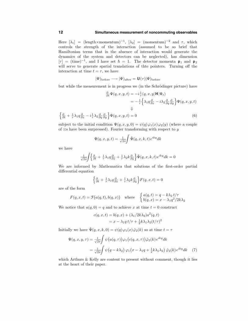
Here ['1] = (length,momentum)!1, ['2] = (momentum)!2 and , , whichcontrols the strength of the interaction (assumed to be so brief thatHamiltonian terms that in the absence of interaction would generate thedynamics of the system and detectors can be neglected), has dimension[, ] = (time)!1, and I have set ! = 1. The detector momenta p1 and p2

will serve to generate spatial translations of thte pointers. Turning o! theinteraction at time t = , , we have

|$)before !- |$)after = U(,)|$)before

but while the measurement is in progress we (in the Schrodinger picture) have""t$(q, x, y, t) = !i 1

! (q, x, y|H |$t)

= ! 1!

-'1q

""x ! i'2

""q

""y

.$(q, x, y, t)

&-""t + 1

! '1q""x ! i 1

! '2""q

""y

.$(q, x, y, t) = 0 (6)

subject to the initial condition $(q, x, y, 0) = !(q)+1(x)+2(y) (where a coupleof .s have been surpressed). Fourier transforming with respect to y

$(q, x, y, t) = 1"2#

8$(q, x, k, t)eikydk

we have

1"2#

8 -""t + 1

! '1q""x + 1

! '2k""q

.$(q, x, k, t)eikydk = 0

We are informed by Mathematica that solutions of the first-order partialdi!erential equation

-""t + 1

! '1q""x + 1

! '2k""q

.F (q, x, t) = 0

are of the form

F (q, x, t) = F5a(q, t), b(q, x)

6where

$a(q, t) = q ! k'2 t/,b(q, x) = x ! '1q2/2k'2

We notice that a(q, 0) = q and to achieve x at time t = 0 construct

c(q, x, t) = b(q, x) + ('1/2k'2)a2(q, t)

= x ! '1q t/, + 12k'1'2(t/,)2

Initially we have $(q, x, k, 0) = !(q)+1(x) +2(k) so at time t = ,

$(q, x, y, ,) = 1"2#

8!

5a(q, ,)

6+1

5c(q, x, ,)

6+2(k)eikydk

= 1"2#

8!

5q ! k'2

6+1

5x ! '1q + 1

2k'1'2

6+2(k)eikydk (7)

which Arthurs & Kelly are content to present without comment, though it liesat the heart of their paper.


Arthurs & Kelly assume plausibly that the initial states of the detectorsare centered-Gaussian:

+1(x) =%

1"2#$1

e!12 (x/$1)

2& 1

2and +2(y) =

%1"

2#$2e!

12 (y/$2)

2& 1

2

To this they bring the ad hoc assumption—which will acquire motivation in thecourse of their argument—that the Gaussians are “balanced” in the sense that"1"2 = 1

4 . Writing "1 = (4"2)–1 = 12

+b (Arthurs and Kelly call b the “balance

parameter”) we have

+1(x) =: 2

&b

;14e!x2/b and +2(y) =

:2b&

;14e!by2

= 1"2#

8+2(k) eikydk

+2(k) =: 1

2&b

;14e!k2/4b

giving

$(q, x, y, ,) = 1"2#

8!

5a(q, ,)

6+1

5c(q, x, ,)

6+2(k)eikydk

= (1/8&3b)14 ·8

!5q ! k'2

6+1

5x ! '1q + 1

2k'1'2

6e!k2/4b eikydk

The '-parameters were introduced for dimensional reasons, but to simplify thenotation we henceforth assume the numerical values of both to be unity; then

= C1(b)·8

!5q ! k

6+1

5x ! q + 1

2k6e!k2/4b eikydk (8)

with C1(b) = (1/8&3b) 14 .21 Write k - - = q ! k to introduce an alternative

variable of integration, get

= C1·8

!(-) +1

5x ! 1

2 (q + -)6e!(q!%)2/4bei(q!%)yd-

/

|$(q, x, y, ,)| = C1·!!!!8

!(-) +1

5x ! 1

2 (q + -)6e!(q!%)2/4be!i%yd-

!!!!

Drawing upon the assumed Gaussian structure of +1(x) we obtain

= C1

: 2&b

;14!!!!8

!(-) exp$! (x ! q)2 + (- ! x)2

2b

'e!i%yd-

!!!!

= C2 exp$! (x ! q)2

2b

'·!!!!8

!(-) exp$! (- ! x)2

2b

'e!i%yd-

!!!!

with C2 = C1 · (2/&b) 14 = (2/&2b) 1

2 .

21 I am indebted to Ray Mayer for the following line of argument (note tapedto my door, 31 October 2012).


The position/momentum operators of the detector system D1 commutewith those of D1, so projective measurements of the pointer positions x and yare compatable (can be performed simultaneously) and it makes sense to speakof the joint distribution P (x, y), which is itself a conditional distribution; wehave

P (x, y) '8

|$(q, x, y, ,)|2dq

= C 22

8exp

$! (x ! q)2

b

'dq ·

!!!!8

!(-) exp$! (- ! x)2

2b

'e!i%yd-

!!!!2

= C3 ·!!!!8

!(q) exp$! (q ! x)2

2b

'e!i q ydq

!!!!2

(9.1)

with C3 = C 22

+&b =

<1/4&3b and where in the final equation I have adjusted

the name - - q of the integration variable.

Had we (so far as S is concerned) elected to work not in the q -representationbut in the p -representation—writing .(p, x, y, t) to describe the state of thecomposite system—the Schrodinger equation (again set ! = '1 = '2 = 1) wouldhave read -

""t ! i 1

!""p

""x ! 1

! p ""y

..(p, x, y, t) = 0

Fourier transforming with respect now to x

.(q, x, y, t) = 1"2#

8.(p, k, y, t)eikxdk

we have -""t + 1

! k ""p ! 1

! p ""y

..(p, k, y, t) = 0

.(p, k, y, 0) = /(p) +1(k) +2(y)

giving (again with Mathematica’s assistance)

.(p, x, y, t) = 1"2#

8/(p ! 1

! kt) +1(k) +2(y + 1! pt ! 1

2!2 kt2)eikxdk

&

= 1"2#

8/(p ! k) +1(k) +2(y + p ! 1

2k)eikxdk at t = ,

Again invoke the assumption that the intitial detector states are Gaussian

+1(k) =:

b2&

;14e!

bk24 and +2(y) =

:2b&

;14e!by2

and obtain (after a change of variables k - p ! - and some simplification)

|.(p, x, y, ,)| = C4

!!!!8

/(-) exp$! b(y + q)2 + b(- + y)2

2

'e!i%xd-

!!!!

= C4 exp$! b(y + p)2

2

'·!!!!8

!(-) exp$! b(- + y)2

2

'e!i%xd-

!!!!


where C4 = b/2&2. Therefore

P (x, y) =8

|.(p, x, y, ,)|2dp

= C5 ·!!!!8

/(p) exp$! b(p + y)2

2

'e!ipxdp

!!!!2

(9.2)

whereC5 = C 2

4

8exp

-! b(y + p)2

.dp =

<b/4&3

and in (9.2) I have again adjusted the name - - p of the integration variable.22Equations (9) say the same thing in di!erent ways.

Assume by way of example23 that initially

!(q) =: 1

2&"2

;14e!q2/4$2

=+

Gaussian

0

/(p) =:2"2

&

;14e!p2$2

Looking to |!(q)|2 and |/(p)|2 we see that the data generated when q and pare subjected to independent projective measurements are expected to havevariances

" 2q = "2 and " 2

p = 1/4"2

We expect by the Heisenberg uncertainty principle to have "q"p $ 12 (recall

! = 1) but in the present instance have "q"p = 12 since !(q) is a minimally

dispersive state. Whether we work from (9.1) or (9.2), we find

P (x, y) = "+

2b&(b + 2"2)

exp$! x2 + 2b"2y2

b + 2"2

'

and verify that==

P (x, y)dxdy = 1. The associated marginal distributions are

Q(x) =8

P (x, y)dy = 1<&(b + 2"2)

exp$! x2

b + 2"2

'

P (y) =8

P (x, y)dx =+

2b"2<

&(b + 2"2)exp

$! 2b"2 y2

b + 2"2

'

22 To obtain the Schrodinger equation (6)—which agrees with Arthurs &Kelly—I have been obliged to introduce a minus sign into the interactionHamiltonian H which is absent from A & K. And because in the momentumrepresentation q becomes !i0p (A & K appear to have overlooked the minussign) I at (9.2) have exp{!b(p + y)2/2} instead of their exp{!b(p ! y)2/2}.

23 This example has been selected because it leads to integrals that can bedone in closed form.


which are in this instance seen to be Gaussian:

Q(x) = 1<2&" 2

x

e!x2/2$ 2x with " 2

x = "2 + 12b

P (y) = 1>2&" 2

y

e!y2/2$ 2y with " 2

y ="2 + 1

2b

2b"2= 1

4

(("2)–1 + ( 1

2b)–1)

So when {q , p} are subjected to a series of simultaneous A&K-measurementsand the resulting detector pointer-positions {x, y} measured projectively, theexpected variances of the latter data are

" 2x = " 2

q + 12b

" 2y = " 2

p + 12b–1

*(10)

Fromd(" 2

x" 2y )

db= b2 ! 4"2

8b2"2= 0 =( 1

2b = "2

we discover (compare "q"p $ 12 ) that

"x"y $ 1 (11)

with equality if and only if the balance parameter b and ! -structure stand inthe tuned relationship b = 2"2.

The product structure that was assumed to pertain initially to $(q, x, y, t)was seen at (8) to have been lost during the course of the dynamical interactionof the system and detectors; the states of S and {D1,D1} have become entangled.At the completion of the A & K measurement that caused the detector pointersto register {xm, ym} the post-measurement state of S is

!after(q ; xm, ym) = N –1$(q, xm, ym, ,) with N =7 8

|$(q, xm, ym, ,)|2dq

912

where by (8)

$(q, xm, ym, ,) = C2 exp$! (xm ! q)2

2b+ iqym

'

·8

!(-) exp$! (- ! xm)2

2b

'e!i%ymd-

The integral is a complex number: call it Aei&. We now have

$(q, xm, ym, ,) = C2 exp$! (xm ! q)2

2b+ iqym

'Aei&

and the normalization factor becomes

N = C2

7 8exp

$! (xm ! q)2

b

'dq

912

A = C2(&b)14 A


giving

!after(q ; xm, ym) =! 1

"b

"14

exp#! (q ! xm)2

2b+ iqym

$· e!i! (12.1)

where the final phase factor is unphysical and can be discarded. Fouriertransforming to the momentum representation, we get

#after(p ; xm, ym) =!

b"

"14

exp#! b(p ! ym)2

2! ipxm

$· ei(xmym!!) (12.2)

where again the phase factor can be discarded. The states (12) are readily seento be normalized:

%|!after(q ; xm, ym)|2dq =

%|#after(p ; xm, ym)|2dp = 1. The

associated probability densities are Gaussian

|!after(q ; xm, ym)|2 =! 1

"b

"12

exp#! (q ! xm)2

b

$(13.1)

|#after(p ; xm, ym)|2 =!

b"

"12

exp&! b(p ! ym)2

'(13.2)

with variances ! 2q = 1

2b and ! 2p = 1

2b –1 that (for a familiar Fourier-analyticreason, nothing more profound) satisfy !q!p = 1

2 .

The idealized projective action of an A -meter can, as we have seen, bedescribed

|!)before !" |!)after = some normalized eigenvector |a) of A

The initial state |!)before is destroyed by the measurement process, and theprepared state |!)after conveys no indication of what |!)before might have been,conceals no “memory” of |!)before.24 Note that the states (12) prepared by theA & K procedure are similar in that regard: they contain no reference to thepre-measurement S-state !(q). Note also that (13) supplies

limb"0

|!after(q ; xm, ym)|2 = $(q ! xm)

limb"0

|#after(p ; xm, ym)|2 = 0

of which the former can be interpreted to refer to the result of a projective

24 From the statistical structure of indefinitely many such measurementsone can constuct estimates of the real numbers |(a|!)before|, but from thatinformation it is still not possible in the absence of all complex phase data toreconstruct

|!)before =(

|a)da(a|!)before

E!orts to “measure the quantum state of S” would appear therefore to be funda-mentally misguided unless one is prepared to bring into play ideas and methodsthat lie beyond the reach of the von Neumann formalism. In Ulf Leonhardt’sMeasuring the Quantum State of Light (1997) the method is tomographic.


q -measurement, and the latter to provide indication that after such ameasurement the expected value of p is indeterminate. The situation is reversedin the limit b # $.

The fact that xm and ym enter in distinctive ways into (12.1) is easilyunderstood. At ym = 0 we have

!after(q ; xm, 0) =! 1

"b

"14

exp#! (q ! xm)2

2b

$

= Gaussian wavepacket in q-space

Introduction of the factor exp)iq ym

*serves to “launch” the wavepacket.25

The circumstance that q and p enter jointly into the A & K formalismbrings to mind Wigner’s “phase space formulation of quantum mechanics,”wherein to every !(q) is associated a “Wigner quasi-distribution”26

P"(q, p) = ("!)–1(

!#(q + %) e2 i! p# !(q ! %) d%

Feeding (10.1) into the integral (with ! again set to unity) we compute

= " –1 exp#! (q ! xm)2

b

$ (exp

#! %2 ! i2b(p ! ym)%

b

$d%

= exp#! (q ! xm)2

b! b(p ! ym)2

$(14)

which could hardly be prettier. We verify that%%

P"(q, p)dqdp = 1 and observethat the Wigner distribution (14) is in fact a proper distribution: it becomesnowhere negative. The distribution (14) is encountered at (30) on page 14 ofthe notes just cited26 and at (3.35) on page 48 of Leonhardt’s monograph.24

The Arthurs/Kelly paper provides a solitary reference to the literature,that being to vonNeumann’s Mathematical Foundations ofQuantumMechanics.Quoting from their introductory paragraph, “Just as von Neumann uses an idealmeasurement together with an interaction to explain an indirect observation, weuse ideal measurements together with interactions to explain the simultaneousmeasurement of an observable and its conjugate.” The argument to which theyallude appears on the final three pages of von Neumann’s classic monograph, atthe end of his Chapter VI: “The Measuring Process.” I provide now an accountof von Neumann’s argument, phrased so as to facilitatte comparison with theargument devised by Arthurs & Kelly.

Write "(q, x, t) to describe the devolving state of the composite systemthat consists of S (initial state !(q)) and a solitary detector D (initial state#(x1)). The dynamical interaction is driven by a Hamiltonian of the form

25 See (25) page 9 in my “Gaussian wavepackets” (1998).26 See Advanced Quantum Topics (2000), Chapter 2, page 10.


H = ! 1$ q % p1

The Schrodinger equation27 reads i&t" = ! 1$ q(i&x)" or

)&t + 1

$ q&x

*" = 0

solutions of which are of the form F+q, x! 1

$ q t,, which at t = 0 becomes F

+q, x

,.

So"(q, x, t) = !(q)#

+x ! 1

$ q t,

&= !(q)#(x ! q) at t = '

in which the S and D variables have become entangled. Assume that the initial(pre-measurement) states !(q) and #(x) normalized. Then

|"(q, x, 0)|2 = 1 !!!!!!!!!!!!!!!!"evolution is unitary

|"(q, x, t)|2 = |!(q)|2 · |#(x ! q)|2 = 1

and the marginal q -probability is

P (q) = |!(q)|2(

|#(x ! q)|2dx = |!(q)|2

von Neumann remarks parenthetically that because q and x are continuous theycan be measured “with arbitrary but not with absolute precision.” Suppose #(x)is—like (say) a narrow Gaussian—non-zero only in the immediate neighborhoodof the origin (!$ < x < +$). Suppose, moreover, that a projective inspectionof the detector at time ' shows the pointer to be at xm. We can conclude thatthe post-measurement probability density |!after(q)|2 is localized at q ' xm

( xm+%

xm!%|!after(q)|2 dq ' 1

and that the prepared state !after(q) of S is of the form

!after(q) = f(q) i!(q)

where concening the localized function we know only that

( xm+%

xm!%f2(q)dq '

( +$

!$f2(q)dq = 1

while ((q) remains entirely undetermined.

27 I write p1 to distinguish the momentum of D from that of S, but will dropthe pedanatic subscript from x1. As has been our custom, we set ! = 1, thoughin the present instance the ! -factors would cancel anyway.


Abstract essentials of theArthurs/Kelly formalism. Familiarly, one cannot assignsimultaneously precise values to the position and momentum of a quantumstate because [q , p ] (= 0 .28 Arthurs & Kelly, building upon the frameworkerected by von Neumann, looked therefore to the construction of states to whichsimultaneously imprecise position/momentum values can be assigned in a best-possible way.29 In the final paragraphs of their paper they sketch an abstractgeneralization of their simultaneous measurement procedure. Leonhardt, in§6.1.1 of Chapter 6 (“Simultaneoous measurment of position and momentum”)in the monograph previously cited,24 presents a clarified paraphrase of the A/Kargument upon which I base the following remarks.

Introduce near-variants of q and p

Q = q + A

P = p + B

where the “noise terms” A and B model the imprecision which we propose tointroduce into the measurement process. Impose upon {Q , P} the simultaneousmeasureability requirement [Q , P ] = [q , p ]+[q , B ]+[A , p ]+[A , B ] = 0 , which(recall ! = 1) we write

[A , B ] = !i I ! [q , B ] ! [A , p ] (15)

Look now to the noisy analog #2Q#2P of #2q#2p ) 14 . We have

#2Q =-(q + A)2

.!

-q + A

.2

=-q2

.!

-q.2 +

-q A

.!

-q.-

A.

+-A q

.!

-A

.-q.

+-A2

.!

-A

.2

and if we impose upon the noise operator A the (plausible?) assumption thatfor all states *A+ = *q A+ = *A q+ = 0 obtain (compare (10))

#2Q = #2q +-A2

.(16.1)

Similarly#2P = #2p +

-B2

.(16.2)

Therefore

#2Q#2P = #2q #2p + 2#2q

-B2

.+ #2p

-A2

.

2+

-A2

.-B2

.

Leonhardt draws at this point upon the fact the if a and b are non-negative realnumbers then

a + b2

),

ab : “arithmetic mean dominates geometric mean”

with equality if and only if a = b (this is the simplest instance of a large class

28 That statement pertains, of course, to any pair (or expanded set) of non-commutative observables, whether or not they happen to be “conjugate” in thesense [A , B ] = i I .

29 Look back, in this light, to (12).

Abstract essentials of the Arthurs/Kelly formalism 21

of lovely inequalities of which the Wikipedia article “Inequality of arithmeticand geometric means” provides a good account) . . . to write

#2Q#2P ) #2q #2p + 2 #q#p/-

A2.-

B2.

+-A2

.-B2

.

=0#q #p +

/-A2

.-B2

. 12

-

#Q#P ) 12 +

/-A2

.-B2

.

with equality if and only if #2q-B2

.= #2p

-A2

.. Retaining the presumption

that *A+ = *B+ = 0 we have #2A =-A2

.and #2B =

-B2

., so by Schrodinger’s

inequality (1.1)-A2

.-B2

.)

2[A , B ]

2i

32

which by (15) becomes

=0!

-i I

.!

-[q , B ]

.+

-[p , A ]

.

2i

12

=4! 1

2 ! 0 + 052

= 14 (17)

giving

#Q #P ) #q #p + 12 (18)

) 1

We have here reproduced—by a relatively more abstract/general line ofargument—a fundamental result that on page 16 was phrased )x)y ) 1. Itserves to quantify the price one necessarily pays for simultaneous measurement.

The quantum states (12) that result from application of the A/K modelof a simultaneous measurement process are “minimal dispersion” states, in thesense mentioned on page 7. They give rise to Wigner distributions (14) thatserve via

b–1(x ! xm)2 + b(p ! ym)2 = constantto inscribe {xm, ym}-centered curves on phase space—curves that are circularif b = 1 and otherwise elliptical (“squeezed”). Noting the structural similarityof (10) and (16), we observe the the product of the dangling terms in (10) is( 12b)( 1

2b–1) = 14 while the associated product in (16) is (in the optimal case:

see (17))-A2

.-B2

.= 1

4 . Since the shape of the Wigner ellipse is controlledby b =

6( 12b)/( 1

2b–1)71/2 it becomes natural to assign similar significance to the

ratio6-

A2.8-

B2.71/2, which by Leonhardt’s optimality condition #2q

-B2

.=

#2p-A2

.becomes

6#q/#p

71/4. And indeed, what Leonhardt and others callthe “sqeezing parameter” is defined

* = 14 log(#p/#q) = 1

4 log+-

B2.8-

A2.,

= 0 in the circular case (no sqeezing)


Simultaneous measurements of conjugate observables are necessarilyimperfect measurements. The question arises: Can the formal devices employedby Arthurs and Kelly be used to describe imperfect measurements of a singleobservable—a noisy von Neumann process? Write

Q = q + A

-Q2 = q2 + q A + A q + A2

Assume (as Arthurs/Kelly did) that *A+ = *q A+ = *A q+ = 0 for all |!). Then

#2Q = #2q + #2A

Such a theory is too impoverished to set a natural bound on #2A. And it exposeswith stark clarity a problem that bedevils also Arthurs/Kelly’s formal theory ofsimultaneous measurement: If (as was implicitly assumed at every step, as whenwe appealed to Schrodinger’s inequality) A refers to a self-adjoint operator

A =(

|a)a da(a|

then how is it possible to achieve *A+ = 0 for all |!)? That would require thatevery |!) lies in the null space of A (e!ectively: A = 0), and would entail

#2A = *A2+ = 0

I am inclined, therefore, to dismiss Arthurs/Kelly’s formal theory as a suggestivehoax, a provocative idea that stands in need of more careful development.Curiously, the fundamental defect to which I have drawn attention does notappear to o!end Leonhardt, whose frequent reference to “fluctuations” seemsintended to forgive all sins.

Arthurs/Kelly’s dynamical model is susceptible to criticisms of a di!erentsort. Since presented as the analysis of an idealized “gedanken experiment,” wecan dismiss as irrelevant the circumstance that A/K provide no indication ofhow their interaction Hamiltonian might be realized physically, or of how theinteraction is to be switched o! at time t = ' .30 More significantly, their ad hocassumption that the initial detector states are balanced Gaussians remains—though central to the analytical details of their paper—quite unmotivated.

Construction of conjugate pairs & the number-phase problem. Can Arthurs/Kelly’s gedanken experiment be realized as a physical experiment? In apedagogical paper—valuable not least for its extensive bibliography, and inwhich no actual experimental results are reported—Michael Raymer31 shows

30 The latter criticism can be made also of von Neumann’s model, and ofmany theoretical contributions to the quantum computation literature.

31 “Uncertainty principle for joint measurement of noncommuting variables,”AJP 62, 986-993 (1994).

Construction of conjugate pairs & the number-phase problem 23

how a simple single slit set-up might be used to accomplish a simultaneousmeasurement of position and momentum. Raymer emphasizes that suchmeasurements are necessarily imprecise measurements. He proceeds withoutexplicit reference to the Hamiltonian-generated interaction of system (in thisinstance a projected particle) and detectors by means of a formalism that is, asit happens, quite similar in its essentials to the formalism I once had occasionto sketch,32 but which he works out in much greater detail than I attempted,and carries to a point where he becomes able establish contact with Arthurs &Kelly.

Quantum optics provides the conceptual and experimental apparatus thatis used most commonly to probe the foundations of quantum theory.33 Itis, therefore, not surprising that Leonhardt devotes the greater part of hisfinal Chapter 6 (“Simultaneous measurement of position and momentum”)to discussion of some relevant quantum optical issues. Central to quantumoptical theory are non-hermitian operators {ak, ak

+} that permit one to movearound in the Foch space of quantum field modes. Those operators satisfycommutations relations of a form [a , a+] = I identical to the [W , W+] = Isatisfied by operators that were encountered already on page 4. Running inreverse the remark that motivated the introduction of W , we observe that thehermitian operators

q = 1%2(W+ + W) and p = i 1%

2(W+ ! W)

are conjugate[q , p ] = i I

and (when decorated with suitably-dimensioned factors) can be interpreted tocomprise “position” and “momentum” operators in whatever context they arise.In quantum optics one writes

X1 = 1%2(a+ + a) and X2 = i 1%

2(a+ ! a)

and calls {X1, X2} “quadrature operators.”34

32 “Quantum measurement with imperfect devices,” notes for a Reed CollegePhysics Seminar presented 16 February 2000. See also my “First steps towarda theory of imperfect meters” on pages 10-11 in “Generalized QuantumMeasurement: Imperfect Meters and POVMs” (September 2012).

33 Raymer—prolific founding director of the Oregon Center for Optics—isa leading experimentalist in the field, which may account for his interest inthe work of Arthurs & Kelly; shortly before the 1996 AJP paper was writtenhe and his group had completed some trail-blazing in a closely related area:see M. Beck, D. T. Smithey, J. Cooper & M. G. Raymer, “Experimentaldetermination of number-phase uncertainty relations,” Opt. Lett 18, 1259(1993); “Measurement of number-phase uncertainty relations of optical fields,”Phys. Rev. A 48, 3159 (1993).

34 See, for example, C. Gerry & P. Knight, Introductory Quantum Optics(2005), page 17. The X i are, in e!ect, conjugate coordinates of the “fieldoscillators” (oscillatory field modes).


Experimentalists—whether they propose to proceed quantum optically ofmechanically—might look to established uncertainty relations

position -momentumtime -energy

angle -angular momentumphase -number

for contexts within which to work. Relatedly, they might notice that conjugateoperators q and p can be used to construct conjugate pairs

Q = Q(q , p) and P = P (q , p)

in a seemingly infinitely many ways, of which some will be more useful thanothers. For example,

[q , p ] = i I =.#

[Q , P ] = i I with Q = q + f(p), P = p[Q , P ] = i I with Q = q , P = p + g(q)

But Weyl showed long ago that it all realizations of the fundamentalcommutator are unitarily equivalent: it is always possible to write

Q = U q U –1, P = U p U –1 with U unitary

(good news, since otherwise quantum mechanics would split into disjointfragments). If, for example, we set U = eiG(q ) we get Q = q and P =p + G&(q). There are, however, aspects of the {q , p} !" {Q , P} process thatmerit closer scrutiny. Here, since commutators become Poisson brackets in theclassical limit, the classical theory of canonical transformations provides usefulguidance. Look, for example, to the Hamiltonian dynamics of a free particle:H(q, p) = 1

2mp2. Energy E is conserved, H(q, p) = E inscribes a curve (actuallya straight line of constant p =

,2mE ) on the phase plane, along which the state

point moves with constant velocity v =9

2E/m, so

T (q, p) = transit time {0, p} !" {q, p}

= q92E/m

= mq/p

Looking to the “time-energy bracket” (analog of the “position-momentumbracket35)

[T (q, p), H(q, p)] = &T&q

&H&p

! &H&q

&T&p

we find by computation that T (q, p) and H(q, p) are conjugate observables:

[T (q, p), H(q, p)] = 1

35 Note that dimensionally [time · energy] = [length · momentum] = [action].


We are motivated by this result to introduce quantum observables36

H = 12m p2 and T = m 1

2 (q p –1 + p –1 q)

where we have used the simplest means to “hermitianize” T . Drawing formallyupon the identity [A , B C ] = [A , B ]C + B [A , C ] we compute

[T , H ] = [q , p ] = i I

This attractive result is, however, subject to several serious criticisms. In thefirst place, we have too casually assumed that [p2, pn] = 0 remains valid evenwhen n < 0. In the Schrodinger representation we expect to have p –1 =

% q,or actually p –1 =

% qa since indefinite integrals are defined only to within an

additive constant. But

&q

( q

af(q)dq !

( q

a&qf(q)dq = f(a)

so [p , p –1]f(q) = 0 pertains only to functions that vanish at the fiducial point:f(a) = 0. More generally, [pn, p –1]f(q) = 0 i! f (n!1)(a) = 0. And we confrontalso a second problem: for H and T to be of any quantum mechanical utilitythey must be self-adjoint. From

&(!&#) ! &(#&!) = !&2# ! #&2!

we see that H is self-adjoint (!|H#) = (#|H!) only with respect to functionsthat satisfy boundary conditions that insure

( b

a

)&(! &#) ! &(#&!)

*dq =

)! &# ! #&!

*:::b

a= 0

which is achieved most simply (and most commonly) by imposition of periodicor box boundary conditions. The self-adjointness of the time operator Timposes, however, a condition( b

a!(q)

0q

( q

a#(x)dx+

( q

ax #(x)dx

1dq =

( b

a#(q)

0q

( q

a!(x)dx+

( q

ax !(x)dx

1dq

the implications of which are much more obscure, but which appears on its faceto be much more restrictive. Moreover, T |') = +|') in the q-representationreads 0

q

( q

a'(x)dx +

( q

ax '(x)dx

1= +'(q)

-2q ' &(q) + 3'(q) = +' &&(q)

36 It is my dim recollection that the following T operator was considered longago by Bohm and Aharanov.


Mathematica reports that solutions are linear combinations

'(q) = c1HermiteH[! 32 , q/

,+] + c2Hypergeometric1F1[ 34 , 1

2 , q2/+]

of Hermite “polynomials” of a negative fractional order and of a certainconfluent hypergeometric function. But both are seen when plotted to betoo unruly to make sense of. And anyway, what meaning could one attachto a temporal eigenvalue, or a temporal eigenfunction? Pretty clearly, theconditions which insure the self-adjointness of H do not—even in this simplest ofcases—imply the automatic self-adjointness of T . We therefore cannot concludefrom Schrodinger’s inequality that #H#T ) 1

2!.

Look more generally to the classical system

H(q, p) = 12mp2 + U(q)

Energy conservation E = 12mq2 + U(q) leads to the transit-time construction37

(dt =

/m2

(19

E ! U(x)dx

which motivates the definition

T (q, p) =/

m2

( q 19H(q, p) ! U(x)

dx

Computation now as before supplies [T (q, p), H(q, p)] = 1. In the associatedquantum theory we have H = H(q , p) = 1

2m p2+U(q), but the specific meaningof

T =/

m2

( q 19H(q , p) ! U(x) I

dx

is not obvious,38 nor is it clear how one would undertake to demonstrate theconjugacy of {T , H}. It is, however, already clear that we cannot expect T tobe self-adjoint with respect to the functions that render H self-adjoint.

Look now more particularly to the classical oscillator: U(q) = 12m,2q2.

From E = 12mp2 + 1

2m,2q2 we see that at the turning points (where p = 0 andthe energy is entirely potential) E = 1

2m,2a2 where a is the amplitude of theoscillation. The transit time 0 " q / a is

T (q, p) =/

m2

( q

0

1/H ! 1

2m,2x2dx

::::H= 1

2m p2+ 12 m&2q2

= 1, arctan(m, q/p)

37 See my Classical Mechanics (1983/84), page 269.38 The Weyl transform (see Advanced Quantum Topics (2000), Chapter 2,

pages 4-7) supplies one possible way to proceed T (q, p)"T , but while attractivein principal it looks to be unworkable in the present general context.


Set m = , = 1 to reduce notational clutter, get

H(q, p) = 12 (q2 + p2)

T (q, p) = arctan(q/p)

and verify that the Poisson bracket [T, H ] = 1. The equations

H(q, p) = constant and T (q, p) = constant

inscribe circles/rays on the phase plane, so the canonical transformation

{q, p} !" {T (q, p), H(q, p)}

is in e!ect a transformation from Cartesian to polar coordinates. Oscillators are“clocks,” in the sense that the moving phase point {q(t), p(t)} traces a circular(generally elliptical) orbit with constant (energy-independent) angular velocity;Hamilton’s canonical equations d

dtA = [A, H ] supply

ddtT = [T, H ] = 1 =. Tt = T0 + t

so in this context “time” and “angle” are equivalent notions.39 Useful insightinto the origin of the conjugacy statement [T, H ] = 1 follows from theobservation that if %(q, p) = q/p then

[%, H ] = 1 + %2

More generally, we have—either by direct calculation or by appeal to the generalidentity [A, g(B)] = [A, B]g &(B)

[%n, H ] = n(%n!1 + %n+1) : n = 1, 2, 3, . . .

We have arctan % = % ! 13%3 + 1

5%5 ! 17%7 + · · · =

;$n=0(!)n 1

2n+1% 2n+1 so

[;N

n=0(!)n 12n+1% 2n+1, H ] = 1 + (!)N% 2N+2

While limN'$

(expression on the left) = [arctan %, H], it would be di$cult to arguethat the expression on the right " 1. This appears to comprise yet anotherindication that time/angle observables are pathological beasts.

Turning now to the associated quantum theory,40 from

q = 1%2(a+ + a)

p = i 1%2(a+ ! a)

<0.

=a = 1%

2(q + ip)

a+ = 1%2(q ! ip)

39 When we reinstate the dimensioned physical parameters {m, ,} we getTt = T0 + , t; “time” and “angle” become dimensionally distinct, but retaintheir proportionality.

40 I borrow material from pages 4–7, but with notation adjusted

{A , B , W , W+} " {q , p , a , a+}

to conform to quantum optical convention.


we haveN = a+a = 1

2 (q2 + p2 ! I) = H ! 12 I = a a+ ! I

which di!ers from H only by an additive (zero-point energy) term, and inquantum optical (bosonic quantum field-theoretic) contexts is called the“number operator.” It’s eigenvalues n = {0, 1, 2, . . .} indicate how many fieldquanta occupy the mode in question. The conjugate operator " is interpretedto refer not to “time” but to angular “phase.” One might expect to be able towrite

[", N ] = i I with " = arctan #

# = 12 (q p –1 + p –1 q)

but several serious problems immediately arise: (i ) The meaning of

p –1 = !i%

2(a+ ! a)–1

is unclear. (ii) To lend meaning to the symbol arctan # we might write

arctan # = limN'$

N>

n=0

(!)n 12n+1 # 2n+1

but then confront

[", H ] = limN'$

N>

n=0

(!)n 12n+1 [# 2n+1, H ]

Iteration of the general identity [A , B C ] = [A , B ]C + B [A , C ] supplies

[# 2n+1, H ] =2n>

k=0

# k[#, H ]# 2n!k

Non-commutivity has produced here such a mess that it appears to be unfeasibleto demonstrate even formally (convergence questions aside) that [", H ] = i I .(iii) If " is so complicated as it now appears to be then proof (in whateversense turns out to be meaningful) of the self-adjointness of " appears to bequite out of the question.

Many attempts to solve the “phase operator problem” have been devisedover the years.41 I mention only one. In the paper42 in which Dirac reportedhis first attempt to construct a quantum electrodynamics he assumed that it ispossible to write

a+ =,

N ei! 0. a = e!i!,

N (19)

41 For an exhaustive review, see P. Carruthers & M. M. Nieto, “Phase andangle variables in quantum mechanics,” Rev. Mod. Phys. 40, 411-440 (1968).A very nice brief account can be found in §2.7 of Gerry & Knight.31

42 Proc. Roy. Soc. (London) A114, 243 (1927).


which presumes "+ = ". Then a+a = N while a a+ ! a+a = I becomes

e!i! Nei! ! N = I

giving e!i! N ! Ne!i! = e!i!. Expand the exponentials and get

! i[", N ] ! 12! ["

2, N ] + i 13! ["

3, N ] + 14! ["

4, N ] ! · · ·= I ! i" ! 1

2!"2 + i 1

3!"3 + 1

4!"4 ! · · ·

Identification of the leading terms supplies

[", N ] = i I

from which it follows that ["k, N ] = ik"k!1, which serve to establish

kth term on left = kth term on right : k = 2, 3, 4, . . .

Dirac’s argument achieves its elegance by postulating the existence of hermitianoperators

,N and " such that a+ =

,N ei!, but has nothing to say about their

explicit construction and supplies no explicit proof of self-adjointness. And, aswas first pointed out by L. Susskin & J. Glogower,43 Dirac’s argument leads tocontradictions. The root problem, as I see it, is that ei! = N! 1

2 a+ requiresN! 1

2 a+ to be unitary. Buta N –1 a+ (= I

because N =;$

0 |n)n(n| and N |0) = 0 imply that N is singular: N –1 does notexist. Dirac’s assumption (19) is untenable.

The short of it is this: In the absence well-defined self-adjoint “time” and“phase” operators T and "—conjugate respectively to the Hamiltonian andnumber operators H and N —it is impossible to construe statements of the forms#E#T ) 1

2! and #N #- ) 12! to be instances of Schrodinger’s inequality.

And it certainly impossible to contemplate the “simultaneous measurement”of energy/time or number/phase. Indeed, it is impossible to speak of “timemeasurements” or “phase measurements” in any standard quantum mechanicalsense. The above uncertainty relations—which (particularly the former) areof undeniably great practical importance—must arise from considerations andprocedures entirely separate from those of quantum measurement theory.33The problems that bedevil the construction of T and " have been seen to beessentially identical. It is—when one thinks about it—not clear what it wouldmean to “measure T ,” and is presumably equally unclear what it would meanto “measure "”: the announcements of detectors are spectrally based, and inthe absence of an operator there is no spectrum. For a recent contribution to

43 Physics 1, 49 (1964). J. S. Bell published his “On the Einstein PodolskyRosen paradox” on pages 195-200 in the same volume of that now-defunctjournal.


to the quantum theory of time operators, see C. M Bender & M. Gianfreda,“Matrix representation of the time operator.44 Michael Nieto45 has provideda useful (if amusingly informal) summary of the substance and recent history(through 1992) of work on the quantum phase problem.

One final remark before we take leave of this topic: It is interesting thatthe classical theory of angle variables (London’s “Winklevariablen”) is so muchmore tractable than its quantum counterpart. Look, for example,37 to the3-component of angular momentum

L3 = x1p2 ! x2p1

Introduce angles(3 = arctan(x1/x2).3 = arctan(p1/p2)

and verify by Poisson bracket evaluation that (3 and .3 are both conjugate toL3 : [L3, (3] = [L3, .3] = 1. Therefore #3 = (3 ! .3 commutes with L3:

[L3, #3] = 0

Drawing upon the identity

arctan(a) ! arctan(b) = arctan!

a ! b1 + ab

"

we find#3 = arctan

!x1p2 ! x2p1

x1p1 + x2p2

"

We observe finally that

[(3, .3] = x1p1 + x2p2

(x21 + x2

2)(p21 + p2

2)

44 http://arxiv.org/abs/1201.3838. This 13-page paper is dated 18 Jan 2012.Google reports the existence of quite an extensive time operator literature.

45 “Quantum phase & quantum phase operators: some physics and somehistory,” http://arxiv.org/abs/hep -th/9304036 (8 Apr 1993). Nieto reportsthat Susskind & Glogower’s discovery of the defect in Dirac’s argument wasanticipated by F. London, “Winkelvariable und kanonische Transformationenin der Undulationsmechanik,” Zeitscrhift fur Physik 40,193 (1927). Here again,Google reports the existence of an extensive literature.

Sim ultaneous Measurement - Reed College · Sim ultaneous Measurement of ... b y Arth urs and Kelly...

Documents

Transcript of Sim ultaneous Measurement - Reed College · Sim ultaneous Measurement of ... b y Arth urs and Kelly...