Abstract

In this paper, we propose a new approach to camera

calibration from silhouettes under circular motion with minimal data. We exploit the mirror symmetry property and derive a common homography that relates silhouettes with epipoles under circular motion. With the epipoles determined, the homography can be computed from the frontier points induced by epipolar tangencies. On the other hand, given the homography, the epipoles can be located directly from the bi-tangent lines of silhouettes. With the homography recovered, the image invariants under circular motion and camera parameters can be determined. If the epipoles are not available, camera parameters can be determined by a low-dimensional search of the optimal homography in a bounded region. In the degenerate case, when the camera optical axes intersect at one point, we derive a closed-form solution for the focal length to solve the problem. By using the proposed algorithm, we can achieve camera calibration simply from silhouettes of three images captured under circular motion. Experimental results on synthetic and real images are presented to show its performance.

1. Introduction Camera calibration from uncalibrated image sequences

without using any specific calibration patterns can be classified into two camps; namely, the feature-based and silhouette-based approaches. In the feature-based approach, structure from motion (SfM) algorithm [20] determines the camera information and the 3D structure of the object simultaneously from the feature correspondences. In the silhouette-based approach, the cameras are first calibrated from the object silhouettes and then the volumetric description, intersection [1] or the image-based visual hull (IBVH) [2] techniques are applied for object modeling.

It takes more efforts to calibrate cameras in general motion from silhouettes [18, 19] than feature points. Boyer [19] proposed a quantitative and qualitative criterion for measuring the silhouette consistency from viewing cones

(or named visual cones), but the estimated results heavily depend on the initial parameters. Sinha et al. [18] proposed a camera calibration method from dynamic silhouettes. The key step is to robustly compute the epipolar geometry from two views. Therefore, dynamic silhouettes are needed for providing enough constraints.

Additional constraints on camera motion, such as circular motion, can facilitate the camera calibration. It may seem to be a restriction to assume the camera motion to be circular motion. However, in real applications, such as 3D digitization in digital museum, 3D object reconstruction from a circular motion sequence is a practical and widely used approach for generating 3D models and a number of 3D reconstruction methods focused on circular motion have been proposed, including the feature-based [3,4,5,6,7] and silhouette-based [8,9,12,13,14,15] methods.

In this paper, we deal with the problem of camera calibration from silhouettes under circular motion. Different from previous silhouette-based methods based on surface of revolution (SoR), the proposed approach can be applied with very few sparsely located views to calibrate the cameras. We introduce the concept of mirror symmetry property [16,17] into circular motion and derive the property that images under circular motion share a common homography that relates silhouettes with epipoles. With this property, epipoles can be located directly from the silhouettes and then the remaining camera parameters can be recovered.

In addition, in the degenerate case, when the optical axes of all cameras intersect at one point, for a reference camera, the projection of x-axis direction in an image, or named x-axis vanishing point, is an infinite point, which influences the calibration process. For this degenerate case, we derive a closed-form solution to determine the focal length by using the epipoles between three images captured under circular motion.

This paper is focused on the problem of camera calibration from silhouettes instead of features, thus it is particularly useful when it is difficult to establish accurate feature correspondences from texture-less, transparent, translucent, or reflective objects, such as jadeite material.

The remainder of this paper is organized as follows. We review some previous works in section 2. Section 3

Silhouette-Based Camera Calibration from Sparse Views under Circular Motion

Po-Hao Huang Shang-Hong Lai Computer Vision Laboratory

Department of Computer Science, National Tsing Hua University, Hsinchu, Taiwan {even, lai}@cs.nthu.edu.tw

978-1-4244-2243-2/08/$25.00 ©2008 IEEE

describes the circular motion geometry. In section 4, we present how to apply the mirror symmetry property to formulate the common homography. The proposed camera calibration algorithm from silhouettes under circular motion is described in section 5. Experimental results on both synthetic and real data are given in section 6. Finally, we conclude this paper in section 7.

2. Previous works For camera calibration under circular motion, the

feature-based [3,4,5,6,7] and silhouette-based [8,9,12,13,14,15] approaches have been proposed.

In the feature-based approaches, Fitzgibbon et al. [3] computed the fundamental matrices and trifocal tensors to uniquely determine the rotation angles. The reconstruction is determined up to a two-parameter family. Jiang et al. [4,5] further developed a method that avoids the computation of multi-view tensors to recover the circular motion geometry by either fitting conics to tracked points in at least five images or computing a plane homography from minimally two points in four images. Cao et al. [6] aimed at the problem of varying focal lengths under circular motion with a constant but unknown rotation angle. With the invariance of the essential matrix, the ratio of varying focal lengths can be determined. Zhong and Hung [7] proposed a circular projective reconstruction method.

In the silhouette-based approaches, Mendonca and Cipolla [8] addressed the problem of estimating the epipolar geometry from contours in the affine and circular motion cases. For the circular motion case, the relation between the epipolar tangencies and the image of rotation axis is used to define a cost function. Under the assumption of constant rotation angle, they iteratively minimize the cost function to determine the two common epipoles between adjacent images. Huang and Lai [15] further extended this method to determine the focal length. In [9], Mendonca et al. exploited the symmetry properties of the SoR swept out by the rotating object to obtain an initial guess of image invariants, followed by several one-dimensional searching steps to obtain the epipolar geometry. However, it still requires the knowledge of the camera intrinsic parameters in advance to recover the rotation angles and the object structure. Zhang et al. further extended this method to achieve auto-calibration [12] and formulated the circular motion as 1D camera geometry to achieve more robust motion estimation [13].

Most of the silhouette-based methods are based on the SoR to obtain an initial guess of image invariants, thus it is infeasible to deal with sparsely located images. Wong et al. [10,11] presented a method based on two epipolar tangencies between image pairs to deal with this problem, but it requires the camera intrinsic parameters to be known

in advance and needs to solve a high-dimensional optimization problem with non-trivial initialization. The method described in [15] could deal with this problem to achieve auto-calibration. Nevertheless, it is restricted to the constant interval angle assumption. Recently, Hernandez et al. [14] defined the silhouette coherence that uses the entire visible silhouettes, not only the tangencies, to measure the silhouette consistency. Cameras are calibrated by maximizing the silhouette coherence and good results could be obtained when the errors of the initial interval angles are within 15 degrees. However, a roughly initial guess for camera parameters is still needed.

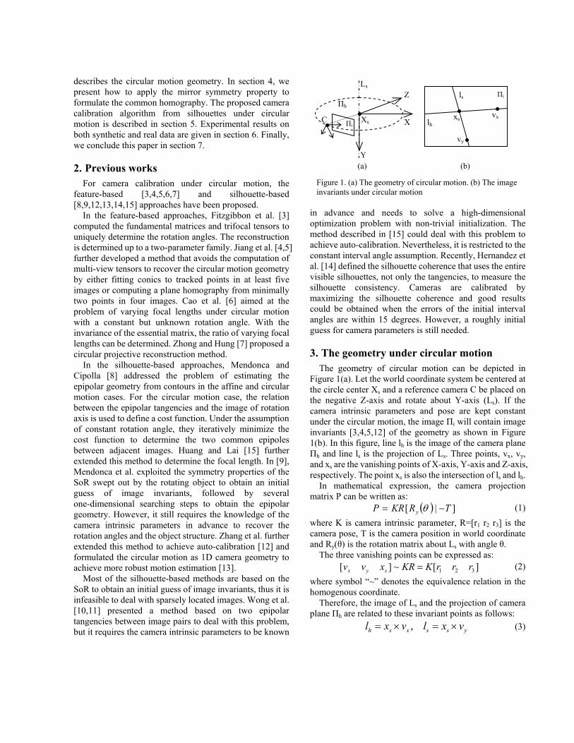
3. The geometry under circular motion The geometry of circular motion can be depicted in

Figure 1(a). Let the world coordinate system be centered at the circle center Xs and a reference camera C be placed on the negative Z-axis and rotate about Y-axis (Ls). If the camera intrinsic parameters and pose are kept constant under the circular motion, the image Πi will contain image invariants [3,4,5,12] of the geometry as shown in Figure 1(b). In this figure, line lh is the image of the camera plane Πh and line ls is the projection of Ls. Three points, vx, vy, and xs are the vanishing points of X-axis, Y-axis and Z-axis, respectively. The point xs is also the intersection of ls and lh.

In mathematical expression, the camera projection matrix P can be written as:

( ) ]|[ TRKRP y −= θ (1)

where K is camera intrinsic parameter, R=[r1 r2 r3] is the camera pose, T is the camera position in world coordinate and Ry(θ) is the rotation matrix about Ls with angle θ. The three vanishing points can be expressed as:

][~][ 321 rrrKKRxvv syx = (2)

where symbol “~” denotes the equivalence relation in the homogenous coordinate. Therefore, the image of Ls and the projection of camera plane Πh are related to these invariant points as follows:

,h s x s s yl x v l x v= × = × (3)

(a) (b)

Xs

Z

Figure 1. (a) The geometry of circular motion. (b) The image invariants under circular motion

Πh

C X

Y

Ls

Πi

Πi

lh

ls

xs

vy

vx

4. Homography from mirror symmetry In this section, we describe how to apply the mirror

symmetry property to derive the plane homography that relates the object contours with epipoles.

4.1. Epipolar geometry from mirror reflection As described in [16,17], the corresponding geometry

established by placing a plane mirror in the scene can be illustrated as a bird’s eye view in Figure 2(a). In the figure, Πm is the mirror plane, X is an object point and its reflection X’ could be imagined as a virtual point at the opposite side of the mirror plane. C represents the real camera with the associated image plane denoted by Πi. Similarly, there exists a virtual camera V on the other side of mirror and its projection onto Πi, which is the epipole denoted by e. Because of mirror reflection, the projection of X’ onto camera C can be regarded as the projection of X onto camera V. Therefore, the two view geometry for a camera with a plane mirror is established.

For simplicity, we denote an object silhouette in the image plane of camera C as SC. In this setting, the image plane Πi contains two silhouettes, real SC and reflected SV, as depicted in Figure 2(b). The major property is that the epipole e can be located by the outer tangent lines of the two silhouettes, SC and SV, and the tangent points, for instance xc and xv, will be considered as the corresponding points (see [16,17] for details).

4.2. Circular motion and mirror reflection The geometry under the setting of plane mirrors is

similar to the circular motion. To be more specific, the relationship is illustrated in Figure 3. In Figure 3(a), C1 and C2 denote two instances of the camera under circular motion. Imagine that there is a plane mirror Πm, which is parallel to and passes through the rotation axis, to be placed in the middle of two camera centers. According to the mirror symmetry property, there is a virtual camera V2, which is the reflection of camera C1 according to Πm, centered at the same position of camera C2. Therefore, we can relate the epipole eC2, which is the projection of C2 onto

C1, with silhouettes SC1 and SV2 by the following equation:

( ) 0212 =×⋅ VCTC xxe (4)

where xC1 and xV2 is a pair of corresponding points from the tangencies of silhouettes SC1 and SV2.

Similarly, camera V2 can be regarded as the reflection of camera C2 according to another mirror plane Πn. To be more specific, we enlarge this part in Figure 3(b). In this figure, Πc and Πv are the image planes of cameras C and V, respectively. Because of the coincident camera center of cameras C and V, silhouettes SC and SV can be transformed with each other via a non-singular 3x3 homography H [20].

From mathematical derivation, the camera projection matrices for cameras C and V can be expressed as:

( ) ]|[ TRKRP yC −= θ (5)

( ) ]|[ TRKRP yV −Σ= θ (6) where Σ = diag([-1 1 1]).

Suppose the projections of an object point X onto cameras C and V are denoted by xc and xv, respectively. The relation between the corresponding image points can be expressed as:

1v c c~ Tx KR R K x Hx−Σ = (7)

The homography H only involves the constant camera intrinsic parameters and camera pose. Thus, all cameras under circular motion share the common homography. Substituting equation (7) into equation (4) leads to

( ) 0212 =×⋅ CCTC Hxxe (8)

Similarly, we can derive the following relation ( ) 0121 =×⋅ CC

TC Hxxe (9)

For any two views under circular motion, a pair of correspondence points with two epipoles can provide two linear constraints on H according to equation (8) and (9). With enough constraints, H can be linearly determined by the least-square estimation.

On the other hand, given the homography H, a silhouette can be transformed to its reflected silhouette. Therefore, the epipoles of any two views can be determined from the bi-tangent lines of one of the silhouettes and the transformed silhouette of the other one.

(a) (b)

C1 C2

V2

Πm

θ

visual cone

Πn

Xs 2θ

C3

C V

ΠcΠv

H

Πn

Figure 3. The geometry relationship between the circular motion and the mirror reflection.

(a) (b)

Πm

Πi

e bi-tangent lines

real silhouette (SC)

reflected silhouette (SV)

X X’

V e C

Figure 2. (a) The bird’s eye view of the two view geometry generate by a plane mirror. (b) Epipole and bi-tangent lines.

xv xc

In addition, equation (8) can be rewritten as follow: ( ) 0][ 221 =× CC

TC xHex (10)

Therefore, the fundamental matrix can be expressed as: HeF C ×= ][ 2 (11)

The derived equations are similar to those in [9,20]. However, the property is derived from the mirror symmetry property. Therefore, we have a new observation that the epipoles of two views under circular motion can be directly located instead of performing one-dimensional search [9].

4.3. Homography and image invariants With the pole-polar relationship, we can show that

s xl vω= (12)

where 1TK Kω − −= is the image of the absolute conic. The homography H derived in the previous section can

be further used to relate to the image invariants as follow:

sTx

TsxTT

lvlvIKrKrIKRKRH 22 1

111 −=−=Σ= −− (13)

Therefore, if there is knowledge about vx or ls, equation (8) and (9) can also be applied to determine the unknown part with a linear solution.

5. Camera Calibration In this section, we discuss how to estimate the camera

parameters by using the proposed property and how to determine the focal length under the degenerate case. We assume the optical centers coincide with the image centers, and the camera intrinsic parameter has only one unknown, i.e. the focal length.

5.1. Recovery of the homography If the epipoles are available, the tangent points of

silhouettes induced by the epipoles are considered as point correspondences, and equation (8) and (9) are used to compute the homography H. One way to extract the epipoles from object silhouettes can be found in [8].

If the epipoles are not available, a low-dimensional search of the optimal H in a bounded region is performed. As given in equation (7), H contains four parameters which are focal length, denoted by f, and three rotation angles, denoted by θx, θy and θz, respectively, of the camera pose. In fact, H is independent of the rotation angle of x-axis because of the following relation:

( ) ( ) Σ=Σ Txxxx RR θθ (14)

Thus, the number of unknowns of H is reduced to three. Under circular motion, all cameras are positioned on the

same plane, which is Πh as shown in Figure 1(a), and their projections, which are epipoles, are co-linear. The homography H can hence be determined by minimizing the

distance from the epipoles to the co-linear line, lh, and the cost function is defined as follow:

( ) ( ) ( )( )( )∑

∈

+=SSS

hjihijzyji

ledistledistfCost ,

,,,, θθ (15)

where the function dist( ) gives the distance from a point to a line, the set S contains all silhouette pairs and eab denotes the epipole which is the projection of camera Cb onto Ca.

As described in section 4.2, the epipoles of a pair of images can be located from a given H and the epipole co-linear line, lh, is computed by a least-square line fitting. Unfortunately, under a given focal length, the error function is complex as shown in Figure 4. Figure 4(a) is the error function of the rotation angles within +/- 20 degrees of the ground truth and Figure 4(b) is that within +/- 1 degree. Thus, the optimization methods will be easily trapped into local minima without very good initialization. However, the values of the unknowns can be bounded within a reasonable range. The optimal H can be searched discretely in a finite parameter spaces.

In practice, a candidate list of H with the cost smaller than a predefined threshold, which can be set to the average cost, will be kept because of the noise. The final solution is chosen with the smallest error in the epipolar tangency constraints, whose detailed description can be found in [10].

5.2. Recovery of the image invariants When the homography H is obtained, the epipoles of a

pair of views can be determined. The line lh is determined via line fitting of epipoles. The line ls is determined via line fitting of the intersections of the corresponding epipolar lines [8]. The point xs hence can be computed from the intersection of lh and ls. The point vx is computed from equation (12) given f and ls or from equation (8), (9) and (13) when the epipoles are available.

5.3. Recovery of the focal length If the homography H is determined via a bounded-search

process, the focal length is therefore determined. If it is determined via given epipoles, with the recovered image

(a) (b)

Figure 4.The error function of different parameters of H.

invariants, vx and ls will provide two constraints to the image of the absolute conic as expressed in equation (12). The focal length can therefore be computed by solving two quadratic equations.

5.4. Recovery of the camera pose From equation (2), camera pose R can be computed by

132

113

111

1,

1,

rrr

xKxKr

vKvKr

ss

xx

×=

±==

±==−−

−−

ββ

αα

(16)

Notice that, the sign of rotation axis has no difference for projection to the image coordinates, but back-projection of image points will lead to a sign ambiguity. This ambiguity can be resolved by back-projecting the epipole, which is obtained from images, and checking the sign with the corresponding camera position. Finally, the overall optimal orthogonalization is done by SVD.

5.5. Recovery of the rotation angle about Ls The inscribed angle theorem of circle states that an

inscribed angle is exactly half the corresponding central angle. As shown in Figure 3(a), we have

23121 2 CCCCXC s ∠=∠ (17) where C3 is an arbitrary camera on the circle.

In this case, the rotation angle about Ls between cameras C1 and C2 can be obtained by calculating the angle between the back-projection lines of the corresponding epipoles of cameras C1 and C2 in the image of camera C3 as follow:

( )21

11

231 , eKeKangCCC −−=∠ (18) where e1 and e2 are epipoles of C1 and C2 in the image of C3.

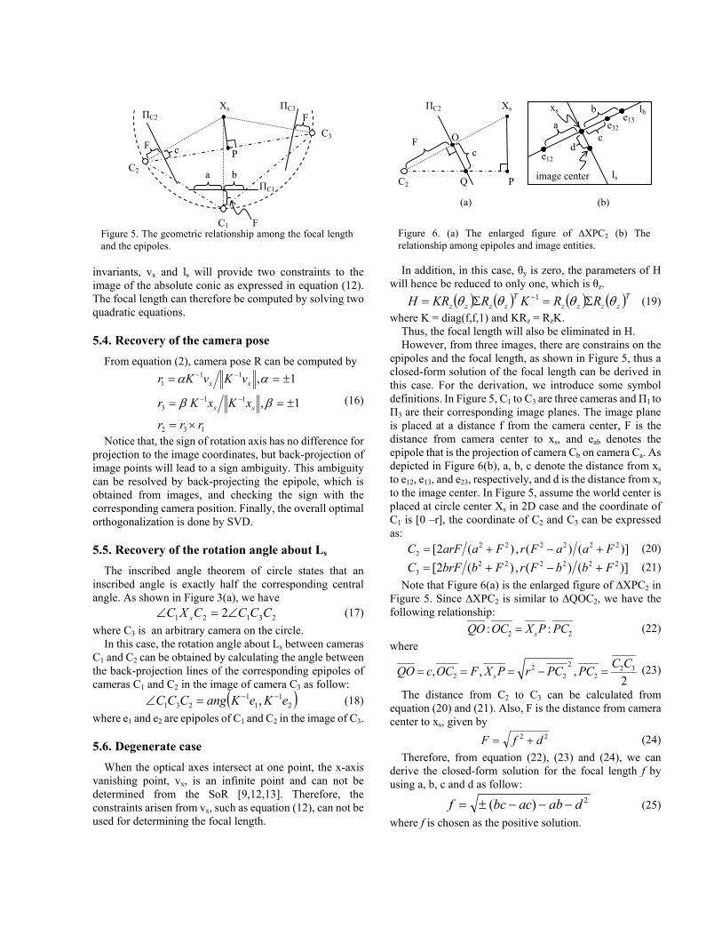
5.6. Degenerate case When the optical axes intersect at one point, the x-axis

vanishing point, vx, is an infinite point and can not be determined from the SoR [9,12,13]. Therefore, the constraints arisen from vx, such as equation (12), can not be used for determining the focal length.

In addition, in this case, θy is zero, the parameters of H

will hence be reduced to only one, which is θz. ( ) ( ) ( ) ( )Tzzzz

Tzzzz RRKRKRH θθθθ Σ=Σ= −1 (19)

where K = diag(f,f,1) and KRz = RzK. Thus, the focal length will also be eliminated in H. However, from three images, there are constrains on the epipoles and the focal length, as shown in Figure 5, thus a closed-form solution of the focal length can be derived in this case. For the derivation, we introduce some symbol definitions. In Figure 5, C1 to C3 are three cameras and Π1 to Π3 are their corresponding image planes. The image plane is placed at a distance f from the camera center, F is the distance from camera center to xs, and eab denotes the epipole that is the projection of camera Cb on camera Ca. As depicted in Figure 6(b), a, b, c denote the distance from xs to e12, e13, and e23, respectively, and d is the distance from xs to the image center. In Figure 5, assume the world center is placed at circle center Xs in 2D case and the coordinate of C1 is [0 –r], the coordinate of C2 and C3 can be expressed as:

])()(,)(2[ 2222222 FaaFrFaarFC +−+= (20)

])()(,)(2[ 2222223 FbbFrFbbrFC +−+= (21)

Note that Figure 6(a) is the enlarged figure of ∆XPC2 in Figure 5. Since ∆XPC2 is similar to ∆QOC2, we have the following relationship:

2 2 : :sQO OC X P PC= (22) where

22 2 32 2 2, , ,

2sC CQO c OC F X P r PC PC= = = − = (23)

The distance from C2 to C3 can be calculated from equation (20) and (21). Also, F is the distance from camera center to xs, given by

22 dfF += (24) Therefore, from equation (22), (23) and (24), we can

derive the closed-form solution for the focal length f by using a, b, c and d as follow:

2)( dabacbcf −−−±= (25) where f is chosen as the positive solution.

Figure 5. The geometric relationship among the focal length and the epipoles.

C1

C2

C3

F

a b ΠC1

ΠC3 ΠC2

F c

Xs

P

F

(a) (b)

Figure 6. (a) The enlarged figure of ∆XPC2 (b) The relationship among epipoles and image entities.

a b

image center

c

ls

d

xs

e12

e32e13

C2 P

Xs ΠC2

Q

O F c

lh

In addition to the case with a rotationally symmetric object, another degenerate case occurs when the contact points of the epipolar planes with the object lie on the rotation axis. In this case, points xc and xv, depicted in Figure 2(b), are identical and the derived constraint cannot be used. However, this problem can be avoided by putting the object away from the rotation axis. The expense is to sacrifice image resolution for the object, which is not a problem for a high-resolution camera.

6. Experimental results In this section, both synthetic and real data are used to

evaluate the proposed algorithm. For each test image sequence, only the silhouettes, instead of feature correspondences, are used for camera calibration.

6.1. Synthetic data In this part, the Stanford bunny model is used to generate

100 data sets to test the algorithm. The model is projected to each image, with the coordinates of all pixels rounded, and then the convex hull algorithm is applied to find the silhouette. Each test set contains 12 images of size 800x600 pixels with interval angle 30 degrees. The value of focal length and the camera pose are randomly generated. The range of f is 1500~5000 pixels, θx is within -10~-50 degrees, θy and θz are within -5~5 degrees. For each test, the number of images used for the reconstruction is randomly chosen from 3 to 6.

The experimental results are shown in Table 1. In this Table, # is the number of images used and Δθi is the average error of the interval angles. The errors of angles are represented in degrees. The error in focal length is computed by taking the focal length difference divided by the ground truth.

For the experiment with the degenerate case, we generate another 100 data sets based on the same setting as the previous ones except fixing θy to 0 degree. In this experiment, the number of images used for reconstruction is set to 3 and the estimated results are listed in Table 2.

6.2. Real data In the experiment on real data set, we provide three kinds

of image sequences. All sequences are sparsely located under circular motion and are not suitable for producing SoR. We applied the proposed algorithm to estimate the camera parameters and then minimized the epipolar tangency constraints [10] for all pairs of views to refine the camera parameters.

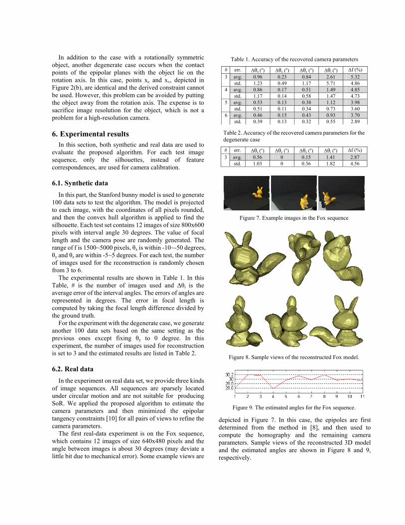
The first real-data experiment is on the Fox sequence, which contains 12 images of size 640x480 pixels and the angle between images is about 30 degrees (may deviate a little bit due to mechanical error). Some example views are

depicted in Figure 7. In this case, the epipoles are first determined from the method in [8], and then used to compute the homography and the remaining camera parameters. Sample views of the reconstructed 3D model and the estimated angles are shown in Figure 8 and 9, respectively.

Figure 9. The estimated angles for the Fox sequence.

Figure 8. Different poses of the constructed 3D model.

Figure 8. Sample views of the reconstructed Fox model.

Figure 7. Example images in the Fox sequence

Table 2. Accuracy of the recovered camera parameters for the degenerate case

# err. Δθx (o) Δθy (o) Δθz (o) Δθi (o) Δf (%)avg. 0.56 0 0.15 1.41 2.87 3std. 1.03 0 0.36 1.82 4.56

Table 1. Accuracy of the recovered camera parameters

# err. Δθx (o) Δθy (o) Δθz (o) Δθi (o) Δf (%)avg. 0.96 0.23 0.84 2.61 5.32 3std. 1.23 0.49 1.17 5.71 4.86 avg. 0.86 0.17 0.51 1.49 4.85 4std. 1.17 0.14 0.58 1.47 4.73 avg. 0.53 0.13 0.38 1.12 3.98 5std. 0.51 0.11 0.34 0.73 3.60 avg. 0.46 0.15 0.43 0.93 3.70 6std. 0.39 0.13 0.32 0.55 2.89

The second experiment is on the crystal apple sequence

as depicted in Figure 10. Notice that the object is made of glass and it is almost impossible to establish feature correspondences in this case. In this part, six images of size 640x480 pixels with different interval angles are chosen. The estimated results are shown in Figure 11 and 12. Figure 12 shows the ground truth angles in black and the reconstructed values in white. We can see the estimated angles are quite close to the true angles.

Finally, we show the experiment on the horse sequence [11], which contains 14 images of size 640x480 pixels. The sequence was taken under an approximately circular motion and the rectified step makes this sequence become a degenerate case. We chose 3 images, as shown in Figure 13, with their optical axes approximately intersecting at a point, for reconstruction. The comparison of the estimated focal length and the ground truth is listed in Table 3.

In Table 3, ‘GT’ means the ground truth, ‘Ini.’ is the focal length estimated by the proposed method, and ‘Opt.’ is the refined focal length estimate after minimizing the overall epipolar tangency error. The error of the initial estimated focal length is about 5.3% compared to the ground truth. Sample views of the reconstructed 3D model are shown in Figure 14. Because it is reconstructed from 3 views only, the results may seem to be rough. In [11], the camera intrinsic parameters are obtained from off-line calibration. For the proposed method, the camera is auto-calibrated.

6.3. Comparison with Other Methods The proposed method is also compared with the methods

proposed in [10] and [12] in the following experiments.

First, the head image sequence in [10] was used for

reconstruction. The sample views of the reconstructed model and the estimated angles are shown in Figure 15(a) and 16, respectively. In [10], the focal length was calibrated off-line, while the proposed method auto-calibrated the camera. The RMS error of interval angles in [10] is 0.2131o and it is 0.1015o by using the proposed method. In addition, we applied the proposed algorithm to four example images of the vase sequence that were directly clipped from [9] and enlarged to the size of 640x480 pixels. The reconstructed model is shown in Figure 15(b) and the comparison of the estimated focal length with [12] and the ground truth is listed in Table 4. As shown in Table 4, our estimated error is about 4% compared to the ground truth. Notice that, we only used 4 clipped and enlarged images to calibrate the camera instead of the original 18 images used in [12]. It is obvious that more correct results could be obtained when more views are used. However, our proposed method can still work well when only very few sparse views are available, while the previous silhouette-based algorithms are not feasible for this kind of sequences.

Figure 13. Images chosen from the horse sequence

Figure 15. Sample views of the reconstructed (a) Head model and (b) Vase model.

(a) (b)

Table 3. Comparison of the recovered focal length with the ground truth for the degenerate case.

Method GT Proposed Ini. Proposed Opt.f 684.98 723.29 664.85

Figure 14. Sample views of the reconstructed horse model.

Figure 12. The estimated interval angles between images

Figure 11. Sample views of the reconstructed Apple model.

Figure 10. Example images in the crystal apple sequence

7. Conclusion In this paper, we introduced the concept of mirror

symmetry property into circular motion and provide a new observation that the epipoles can be located directly from the silhouettes by using the derived homography under circular motion. With this proposed algorithm, the camera can be calibrated from the silhouettes of sparse views, which can be as small as three, under circular motion. This is quite different from the previous silhouette-based methods, which need dense (the interval angle smaller than 20 degrees) and complete (make a turn) image sequences to generate SoR. In addition, we derived a closed-form solution for focal length under the degenerate case when the camera optical axes intersect at one point.

Experimental results on synthetic and real data sets are presented to demonstrate the performance of the proposed algorithm. Although the epipoles and the geometry under circular motion can be well determined for the feature-based methods, the silhouette-based approach has its advantage when the feature correspondences could not be reliably established, which is very common in practice. Previous silhouette-based methods can produce good camera calibration results only with dense views. By using the proposed algorithm, the camera calibration from silhouettes at very sparse views becomes feasible.

Acknowledgements This work was supported by National Science Council, Taiwan, under the grant NSC 96-2221-E-007-043.

References [1] G. G. Slabaugh, W. B. Culbertson, T. Malzbender, and R. W.

Schafer, A survey of methods for volumetric scene reconstruction from photographs, In Proc. Int. Workshop on Volume Graphics, 81-100, 2001.

[2] W. Matusik, C. Buehler, R. Raskar, S. J. Gortler and L. McMillan, Image-based visual hulls, In Proc. SIGGRAPH, 369-374, 2000.

[3] A. W. Fitzgibbon, G. Cross, and A. Zisserman, Automatic 3D model construction for turn-table sequences, In Proc. 3D Structure from Multiple Images of Large-Scale Environments, 155-170, 1998.

[4] G. Jiang, H.T. Tsui, L. Quan, and A. Zisserman, Single axis geometry by fitting conics, IEEE Trans. Pattern Analysis Machine Intelligence, 25(10):1343-1348, 2002.

[5] G. Jiang, L. Quan, H.T. Tsui, Circular motion geometry using minimal data, IEEE Trans. Pattern Analysis Machine Intelligence, 26(6):721-731, 2004.

[6] X. Cao, J. Xiao, H. Foroosh, and M. Shah, Self-calibration from turn-table sequences in presence of zoom and focus, Computer Vision and Image Understanding, 102(3):227-237, 2006.

[7] H. Zhong and Y. S. Hung, Multi-stage 3D reconstruction under circular motion, Image and Vision Computing, 25(11): 1814-1823, 2007.

[8] P. R. S. Mendonca, and R. Cipolla, Estimation of epipolar geometry from apparent contours: affine and circular motion cases, In Proc. Computer Vision Pattern Recognition, 1:9-14, 1999.

[9] P. R. S. Mendonca, K.-Y. K. Wong, and R. Cipolla, Epipolar geometry from profiles under circular motion, IEEE Trans. Pattern Analysis Machine Intelligence, 23(6):604-616, 2001.

[10] K.-Y. K. Wong, P. R. S. Mendonca, and R. Cipolla, Structure and motion estimation from apparent contours under circular motion, Image and Vision Computing, 20(5):441-448, 2002.

[11] K.-Y. K. Wong and R. Cipolla, Reconstruction of sculpture from its profiles with unknown camera positions, IEEE Trans. on Image Processing, 13(3):381-389, 2004.

[12] H. Zhang, G. Zhang, and K.-Y. K. Wong, Auto-calibration and motion recovery from silhouettes for turntable sequences, In Proc. British Machine Vision Conference, 1:79-88, 2005.

[13] G. Zhang, H. Zhang, and K.-Y. K. Wong, 1D camera geometry and its application to circular motion estimation, In Proc. British Machine Vision Conference, 1:67-76, 2006.

[14] C. Hernandez, F. Schmitt, and R. Cipolla, Silhouette coherence for camera calibration under circular motion, IEEE Trans. Pattern Analysis Machine Intelligence, 29(2):343-349, 2007.

[15] P.-H. Huang and S.-H. Lai, Camera calibration from silhouette under incomplete circular motion with a constant interval angle, In Proc. Asian Conference on Computer Vision, 1:106-115, 2007.

[16] K. Forbes, F. Nicolls, G. de Jager and A. Voigt, Shape-from-silhouette with two mirrors and an uncalibrated camera, In Proc. 9th European Conference on Computer Vision, 2:165-178, 2006.

[17] P.-H. Huang and S.-H. Lai, Contour-based structure from reflection, In Proc. Computer Vision Pattern Recognition, 1:379-386, 2006.

[18] S. N. Sinha, M. Pollefeys and L. McMillian, Camera network calibration from dynamic silhouettes, In Proc. Computer Vision and Pattern Recognition, 1:195-202, 2004.

[19] E. Boyer, On using silhouettes for camera calibration, In Proc. Asian Conference on Computer Vision, 1-10, 2006

[20] R. Hartley and A. Zisserman, Mutliple View Geometry, Cambridge University Press, 2000.

Table 4. Comparison of the recovered focal length with the ground truth and the method by Zhang et al. [12].

Method GT Zhang et al.[12] Proposed Opt. # - 18 4 f 2389.8 2370.7 2288.4

Figure 16. The estimated interval angles between images.