Signals and Systems Lecture 7: Laplace Transformele.aut.ac.ir/~abdollahi/Lec_7_S12.pdf · Outline...
48
Outline Introduction Analyzing LTI Systems with LT Geometric Evaluation Unilateral LT Feed Back Applications State Space Signals and Systems Lecture 7: Laplace Transform Farzaneh Abdollahi Department of Electrical Engineering Amirkabir University of Technology Winter 2012 Farzaneh Abdollahi Signal and Systems Lecture 7 1/48
Transcript of Signals and Systems Lecture 7: Laplace Transformele.aut.ac.ir/~abdollahi/Lec_7_S12.pdf · Outline...
Outline Introduction Analyzing LTI Systems with LT Geometric Evaluation Unilateral LT Feed Back Applications State Space Representation
Signals and SystemsLecture 7: Laplace Transform
Farzaneh Abdollahi
Department of Electrical Engineering
Amirkabir University of Technology
Winter 2012
Farzaneh Abdollahi Signal and Systems Lecture 7 1/48
Outline Introduction Analyzing LTI Systems with LT Geometric Evaluation Unilateral LT Feed Back Applications State Space Representation
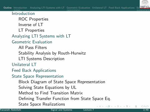
IntroductionROC PropertiesInverse of LTLT Properties
Analyzing LTI Systems with LT
Geometric EvaluationAll Pass FiltersStability Analysis by Routh-HurwitzLTI Systems Description
Unilateral LT
Feed Back Applications
State Space RepresentationBlock Diagram of State Space RepresentationSolving State Equations by ULMethod to Find Transition MatrixDefining Transfer Function from State Space Eq.State Space Realizations
Farzaneh Abdollahi Signal and Systems Lecture 7 2/48
Outline Introduction Analyzing LTI Systems with LT Geometric Evaluation Unilateral LT Feed Back Applications State Space Representation
IntroductionI We had defined est as a basic function for CT LTI systems,s.t.
est → H(s)est
I In Fourier transform s = jω
I In Laplace transform s = σ + jωI By Laplace transform we can
I Analyze wider range of systems comparing to Fourier TransformI Analyze both stable and unstable systems
I The bilateral Laplace Transform is defined:
X (s) =
∫ ∞−∞
x(t)e−stdt
⇒ X (σ + jω) =
∫ ∞−∞
[x(t)e−σt ]e−jωtdt
= F{x(t)e−σt}Farzaneh Abdollahi Signal and Systems Lecture 7 3/48
Outline Introduction Analyzing LTI Systems with LT Geometric Evaluation Unilateral LT Feed Back Applications State Space Representation
Region of Convergence (ROC)
I Note that: X (s) exists only for a specific region of s which is calledRegion of Convergence (ROC)
I ROC: is the s = σ + jω by which x(t)e−σ converges:ROC : {s = σ + jω s.t.
∫∞−∞ |x(t)e−σt |dt <∞}
I Roc does not depend on ωI Roc is absolute integrability condition of x(t)e−σt
I If σ = 0, i,e, s = jω X (s) = F{x(t)}I ROC is shown in s-plane
I The coordinate axes are Re{s} along the horizontal axis and Im{s}along the vertical axis.
Farzaneh Abdollahi Signal and Systems Lecture 7 4/48
Outline Introduction Analyzing LTI Systems with LT Geometric Evaluation Unilateral LT Feed Back Applications State Space Representation
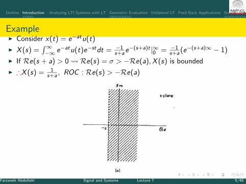
ExampleI Consider x(t) = e−atu(t)
I X (s) =∫∞−∞ e−atu(t)e−stdt = −1
s+ae−(s+a)t |∞0 = −1
s+a(e−(s+a)∞ − 1)
I If Re(s + a) > 0 Re(s) = σ > −Re(a),X (s) is bounded
I ∴X (s) = 1s+a , ROC : Re(s) > −Re(a)
Farzaneh Abdollahi Signal and Systems Lecture 7 5/48
Outline Introduction Analyzing LTI Systems with LT Geometric Evaluation Unilateral LT Feed Back Applications State Space Representation
Example
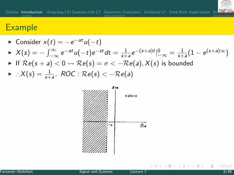
I Consider x(t) = −e−atu(−t)
I X (s) = −∫∞−∞ e−atu(−t)e−stdt = 1
s+ae−(s+a)t |0−∞ = 1
s+a(1− e(s+a)∞)
I If Re(s + a) < 0 Re(s) = σ < −Re(a),X (s) is bounded
I ∴X (s) = 1s+a , ROC : Re(s) < −Re(a)
Farzaneh Abdollahi Signal and Systems Lecture 7 6/48
Outline Introduction Analyzing LTI Systems with LT Geometric Evaluation Unilateral LT Feed Back Applications State Space Representation
I In the recent two examples two different signals had similar Laplacetransform but with different Roc
I To obtain unique x(t) both X (s) and ROC is required
I If x(t) is defined as a linear combination of exponential functions, itsLaplace transform (X (s)) is rational
I In LTI expressed in terms of linear constant-coefficient differentialequations, Laplace Transform of its impulse response (its transferfunction) is rational
I X (s) = N(s)D(s)
I Roots of N(s) zeros of X(s); They make X(s) equal to zero.I Roots of D(s) poles of X(s); They make X(s) to be unbounded.
Farzaneh Abdollahi Signal and Systems Lecture 7 7/48
Outline Introduction Analyzing LTI Systems with LT Geometric Evaluation Unilateral LT Feed Back Applications State Space Representation
I To study the stability of LTI systems zeros and poles are illustrated ins-plane (pole-zero plot)
I number of poles and zeros are equal for −∞ to ∞I Consider degree of D(s) (# of poles): m; degree of N(s) (# of zeros): nI If m < n There are n −m = k poles in ∞I If m > n There are m − n = k zeros in ∞
Farzaneh Abdollahi Signal and Systems Lecture 7 8/48
Outline Introduction Analyzing LTI Systems with LT Geometric Evaluation Unilateral LT Feed Back Applications State Space Representation
ROC Properties
I ROC only depends on σI In s-plane Roc is strips parallel to jω axis
I If X (s) is rational, Roc does not contain any poleI Since D(s) = 0, makes X (s) unbounded
I If x(t) is finite duration and is absolutely integrable, then ROC is entires-plane
I If x(t) is right sided and Re{s} = σ0 ∈ ROC then ∀s Re{s} > σ0 ∈ROC
I If x(t) is left sided and Re{s} = σ0 ∈ ROC then ∀s Re{s} ≤ σ0 ∈ ROC
I If x(t) is two sided and Re{s} = σ0 ∈ ROC then ROC is a strip ins-plane including Re{s} = σ0
Farzaneh Abdollahi Signal and Systems Lecture 7 9/48
Outline Introduction Analyzing LTI Systems with LT Geometric Evaluation Unilateral LT Feed Back Applications State Space Representation
ROC Properties
I If X (s) is rationalI the ROC is bounded between poles or extends to infinity,I no poles of X (s) are contained in ROCI If x(t) is right sided, then ROC is in the right of the rightmost poleI If x(t) is left sided, then ROC is in the left of the leftmost pole
I If ROC includes jω axis then x(t) has FT
Farzaneh Abdollahi Signal and Systems Lecture 7 10/48
Outline Introduction Analyzing LTI Systems with LT Geometric Evaluation Unilateral LT Feed Back Applications State Space Representation
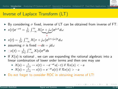
Inverse of Laplace Transform (LT)
I By considering σ fixed, inverse of LT can be obtained from inverse of FT:
I x(t)e−σt = 12π
∫∞−∞ X (σ + jω︸ ︷︷ ︸
s
)e jωtdω
I x(t) = 12π
∫∞−∞ X (σ + jω)e(σ+jω)tdω
I assuming σ is fixed ds = jdω
I ∴x(t) = 12πj
∫∞−∞ X (s)estds
I If X (s) is rational , we can use expanding the rational algebraic into alinear combination of lower order terms and then one may use
I X (s) = 1s+a x(t) = −e−atu(−t) if Re{s} < −a
I X (s) = 1s+a x(t) = e−atu(t) if Re{s} > −a
I Do not forget to consider ROC in obtaining inverse of LT!
Farzaneh Abdollahi Signal and Systems Lecture 7 11/48
Outline Introduction Analyzing LTI Systems with LT Geometric Evaluation Unilateral LT Feed Back Applications State Space Representation
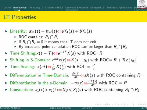
LT Properties
I Linearity: ax1(t) + bx2(t)⇔aX1(s) + bX2(s)I ROC contains: R1
⋂R2
I If R1
⋂R2 = ∅ it means that LT does not exit
I By zeros and poles cancelation ROC can be larger than R1
⋂R2
I Time Shifting:x(t − T )⇔e−sTX (s) with ROC=R
I Shifting in S-Domain: es0tx(t)⇔X (s − s0) with ROC= R +Re{s0}I Time Scaling: x(at)⇔ 1
|a|X ( sa) with ROC = Ra
I Differentiation in Time-Domain: dx(t)dt ⇔sX (s) with ROC containing R
I Differentiation in the s-Domain: −tx(t)⇔dX (s)ds with ROC = R
I Convolution: x1(t) ∗ x2(t)⇔X1(s)X2(s) with ROC containing R1 ∩ R2
Farzaneh Abdollahi Signal and Systems Lecture 7 12/48
Outline Introduction Analyzing LTI Systems with LT Geometric Evaluation Unilateral LT Feed Back Applications State Space Representation
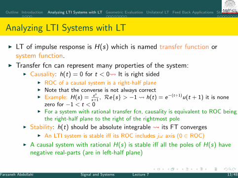
Analyzing LTI Systems with LT
I LT of impulse response is H(s) which is named transfer function orsystem function.
I Transfer fcn can represent many properties of the system:I Causality: h(t) = 0 for t < 0 It is right sided
I ROC of a causal system is a right-half planeI Note that the converse is not always correctI Example: H(s) = es
s+1, Re{s} > −1 h(t) = e−(t+1)u(t + 1) it is none
zero for −1 < t < 0I For a system with rational transfer fcn, causality is equivalent to ROC being
the right-half plane to the right of the rightmost pole
I Stability: h(t) should be absolute integrable its FT convergesI An LTI system is stable iff its ROC includes jω axis (0 ∈ ROC)
I A causal system with rational H(s) is stable iff all the poles of H(s) havenegative real-parts (are in left-half plane)
Farzaneh Abdollahi Signal and Systems Lecture 7 13/48
Outline Introduction Analyzing LTI Systems with LT Geometric Evaluation Unilateral LT Feed Back Applications State Space Representation
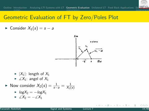
Geometric Evaluation of FT by Zero/Poles Plot
I Consider X1(s) = s − a
I |X1|: length of X1
I ]X1: angel of X1
I Now consider X2(s) = 1s−a = 1
X1(s)
I logX2 = −logX1
I ]X2 = −]X1
Farzaneh Abdollahi Signal and Systems Lecture 7 14/48
Outline Introduction Analyzing LTI Systems with LT Geometric Evaluation Unilateral LT Feed Back Applications State Space Representation
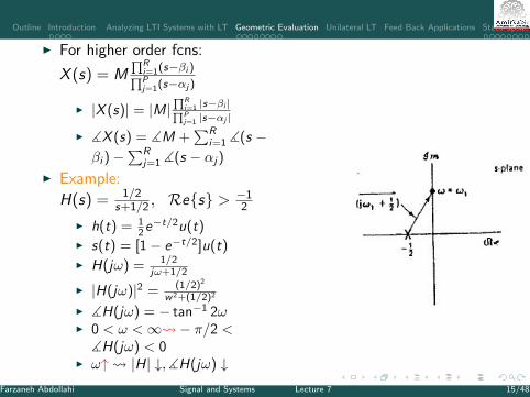
I For higher order fcns:
X (s) = M∏R
i=1(s−βi )∏Pj=1(s−αj )
I |X (s)| = |M|∏R
i=1 |s−βi |∏Pj=1 |s−αj |
I ]X (s) = ]M +∑R
i=1](s −βi )−
∑Rj=1 ](s − αj)
I Example:
H(s) = 1/2s+1/2 , Re{s} >
−12
I h(t) = 12e−t/2u(t)
I s(t) = [1− e−t/2]u(t)I H(jω) = 1/2
jω+1/2
I |H(jω)|2 = (1/2)2
w2+(1/2)2
I ]H(jω) = − tan−1 2ωI 0 < ω <∞ − π/2 <]H(jω) < 0
I ω↑ |H| ↓,]H(jω) ↓Farzaneh Abdollahi Signal and Systems Lecture 7 15/48
Outline Introduction Analyzing LTI Systems with LT Geometric Evaluation Unilateral LT Feed Back Applications State Space Representation
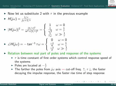
I Now let us substitute 2 with τ in the previous example
I H(jω) = 1/τjω+1/τ
I |H(jω)|2 = (1/τ)2
w2+(1/τ)2 =
1 ω = 01√2
ω = 1τ
1τω ω � 1
τ
I ]H(jω) = − tan−1 τω =
0 ω = 0−π4 ω = 1
τ−π2 ω � 1
τ
I Relation between real part of poles and response of the systemsI τ is time constant of first order systems which control response speed of
the systemsI Poles are located at − 1
τI The farther the poles from jω axis cut-off freq. ↑, τ ↓, the faster
decaying the impulse response, the faster rise time of step response
Farzaneh Abdollahi Signal and Systems Lecture 7 16/48
Outline Introduction Analyzing LTI Systems with LT Geometric Evaluation Unilateral LT Feed Back Applications State Space Representation
Farzaneh Abdollahi Signal and Systems Lecture 7 17/48
Outline Introduction Analyzing LTI Systems with LT Geometric Evaluation Unilateral LT Feed Back Applications State Space Representation
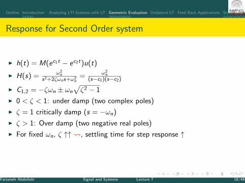
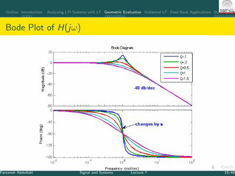
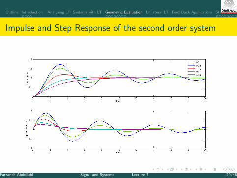
Response for Second Order system
I h(t) = M(ec1t − ec2t)u(t)
I H(s) = ω2n
s2+2ζωns+ω2n
= ω2n
(s−c1)(s−c2)
I C1,2 = −ζωn ± ωn
√ζ2 − 1
I 0 < ζ < 1: under damp (two complex poles)
I ζ = 1 critically damp (s = −ωn)
I ζ > 1: Over damp (two negative real poles)
I For fixed ωn, ζ ↑↑ , settling time for step response ↑
Farzaneh Abdollahi Signal and Systems Lecture 7 18/48
Outline Introduction Analyzing LTI Systems with LT Geometric Evaluation Unilateral LT Feed Back Applications State Space Representation
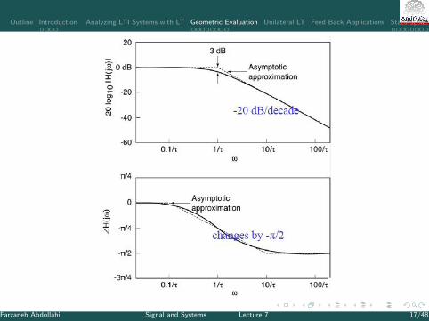
Bode Plot of H(jω)
Farzaneh Abdollahi Signal and Systems Lecture 7 19/48
Outline Introduction Analyzing LTI Systems with LT Geometric Evaluation Unilateral LT Feed Back Applications State Space Representation
Impulse and Step Response of the second order system
Farzaneh Abdollahi Signal and Systems Lecture 7 20/48
Outline Introduction Analyzing LTI Systems with LT Geometric Evaluation Unilateral LT Feed Back Applications State Space Representation
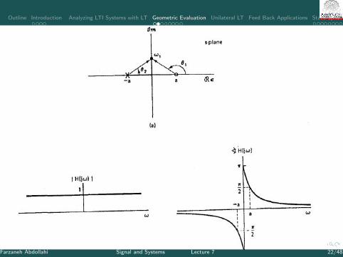
All Pass Filters
I Passes the signal in all freqs. with a little decreasing/increasing themagnitude
I Why do we use all-pass filters?
I H(s) = s−as+a Re{s} > −a, a > 0
I |H(ω)| = 1
I ]H(jω) = θ1 − θ2 = π − 2θ2 = π − 2tan−1(ωa ) =
π ω = 0π2 ω = a0 ω � a
Farzaneh Abdollahi Signal and Systems Lecture 7 21/48
Outline Introduction Analyzing LTI Systems with LT Geometric Evaluation Unilateral LT Feed Back Applications State Space Representation
Farzaneh Abdollahi Signal and Systems Lecture 7 22/48
Outline Introduction Analyzing LTI Systems with LT Geometric Evaluation Unilateral LT Feed Back Applications State Space Representation
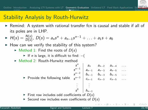
Stability Analysis by Routh-Hurwitz
I Remind: A system with rational transfer fcn is causal and stable if all ofits poles are in LHP.
I H(s) = N(s)D(s) , D(s) = ans
n + an−1sn−1 + . . .+ a1s + a0
I How can we verify the stability of this system?I Method 1: Find the roots of D(s)
I If n is large, it is difficult to find: −(
I Method 2: Routh-Hurwitz method
I Provide the following table
sn an an−2 an−4 . . .sn−1 an−1 an−3 an−5 . . .sn−2 bn−1 bn−3 bn−5 . . .sn−3 cn−1 cn−3 cn−5 . . .
......
s0 hn−1
I First row includes odd coefficients of D(s)I Second row includes even coefficients of D(s)
Farzaneh Abdollahi Signal and Systems Lecture 7 23/48
Outline Introduction Analyzing LTI Systems with LT Geometric Evaluation Unilateral LT Feed Back Applications State Space Representation
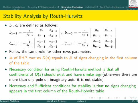
Stability Analysis by Routh-Hurwitz
I bi , ci are defined as follows:
bn−1 = − 1an−1
∣∣∣∣ an an−2
an−1 an−3
∣∣∣∣ , bn−3 = − 1an−1
∣∣∣∣ an an−4
an−1 an−5
∣∣∣∣cn−1 = − 1
bn−1
∣∣∣∣ an−1 an−3
bn−1 bn−3
∣∣∣∣ , cn−3 = − 1bn−1
∣∣∣∣ an−1 an−5
bn−1 bn−5
∣∣∣∣I Follow the same rule for other rows parameters
I # of RHP root os D(s) equals to # of signs changing in the first columnof the table
I Necessary condition for using Routh-Horwitz method is that allcoefficients of D(s) should exist and have similar sign(otherwise there aremore than one pole on imaginary axis, it is not stable)
I Necessary and Sufficient conditions for stability is that no signs changingappears in the first column of the Routh-Horwitz table
Farzaneh Abdollahi Signal and Systems Lecture 7 24/48
Outline Introduction Analyzing LTI Systems with LT Geometric Evaluation Unilateral LT Feed Back Applications State Space Representation
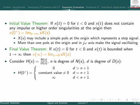
I Initial Value Theorem: If x(t) = 0 for t < 0 and x(t) does not containany impulse or higher order singularities at the origin thenx(0+) = lims→∞ sX (s)
I X (s) may include a simple pole at the origin which represents a step signal.I More than one pole at the origin and in jω axis make the signal oscillating
I Final Value Theorem: If x(t) = 0 for t < 0 and x(t) is bounded whent →∞ then x(∞) = lims→0 sX (s)
I Consider H(s) = N(s)D(s) , n is degree of N(s), d is degree of D(s):
I H(0+) =
0 d > n + 1constant value 6= 0 d = n + 1
∞ d < n + 1
Farzaneh Abdollahi Signal and Systems Lecture 7 25/48
Outline Introduction Analyzing LTI Systems with LT Geometric Evaluation Unilateral LT Feed Back Applications State Space Representation
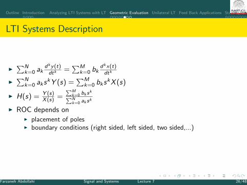
LTI Systems Description
I∑N
k=0 akdky(t)dtk
=∑M
k=0 bkdkx(t)dtk
I∑N
k=0 akskY (s) =
∑Mk=0 bks
kX (s)
I H(s) = Y (s)X (s) =
∑Mk=0 bk s
k∑Nk=0 ak s
k
I ROC depends onI placement of polesI boundary conditions (right sided, left sided, two sided,...)
Farzaneh Abdollahi Signal and Systems Lecture 7 26/48
Outline Introduction Analyzing LTI Systems with LT Geometric Evaluation Unilateral LT Feed Back Applications State Space Representation
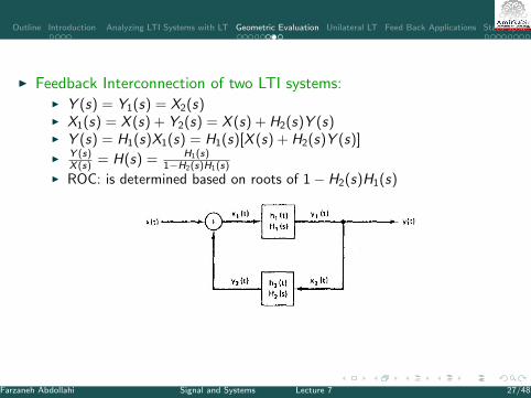
I Feedback Interconnection of two LTI systems:I Y (s) = Y1(s) = X2(s)I X1(s) = X (s) + Y2(s) = X (s) + H2(s)Y (s)I Y (s) = H1(s)X1(s) = H1(s)[X (s) + H2(s)Y (s)]I Y (s)
X (s) = H(s) = H1(s)1−H2(s)H1(s)
I ROC: is determined based on roots of 1− H2(s)H1(s)
Farzaneh Abdollahi Signal and Systems Lecture 7 27/48
Outline Introduction Analyzing LTI Systems with LT Geometric Evaluation Unilateral LT Feed Back Applications State Space Representation
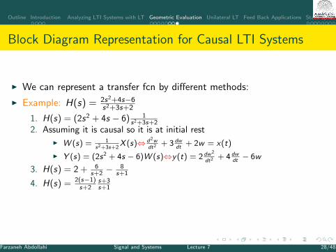
Block Diagram Representation for Causal LTI Systems
I We can represent a transfer fcn by different methods:
I Example: H(s) = 2s2+4s−6s2+3s+2
1. H(s) = (2s2 + 4s − 6) 1s2+3s+2
2. Assuming it is causal so it is at initial rest
I W (s) = 1s2+3s+2
X (s)⇔ d2wdt2 + 3 dw
dt+ 2w = x(t)
I Y (s) = (2s2 + 4s − 6)W (s)⇔y(t) = 2 dw2
dt2 + 4 dwdt− 6w
3. H(s) = 2 + 6s+2 −
8s+1
4. H(s) = 2(s−1)s+2
s+3s+1
Farzaneh Abdollahi Signal and Systems Lecture 7 28/48
Outline Introduction Analyzing LTI Systems with LT Geometric Evaluation Unilateral LT Feed Back Applications State Space Representation
Unilateral LT
I It is used to describe causal systems with nonzero initial conditions:X (s) =
∫∞0− x(t)e−stdt = UL{x(t)}
I If x(t) = 0 for t < 0 then X (s) = X (s)
I Unilateral LT of x(t) = Bilateral LT of x(t)u(t−)
I If h(t) is impulse response of a causal LTI system then H(s) = H(s)
I ROC is not necessary to be recognized for unilateral LT since it is alwaysa right-half plane
I For rational X (s), ROC is in right of the rightmost pole
Farzaneh Abdollahi Signal and Systems Lecture 7 29/48
Outline Introduction Analyzing LTI Systems with LT Geometric Evaluation Unilateral LT Feed Back Applications State Space Representation
Similar Properties of Unilateral and Bilateral LTI Convolution: Note that for unilateral LT, If both x1(t) and x2(t) are zero
for t < 0, then X (s) = X1(s)X2(s)
I Time Scaling
I Shifting in s domain
I Initial and Finite Theorems: they are indeed defined for causal signals
I Integrating:∫ t
0− x(τ)dτ = x(t) ∗ u(t)UL⇔X (s)U(s) = 1
sX (s)I The main difference between UL and LT is in time differentiation:
I UL{ dx(t)dt } =
∫∞0−
dx(t)dt e−stdt
I Use the rule∫fdg = fg −
∫gdf
I ∴UL{ dx(t)dt } = s
∫∞0− x(t)e−stdt + x(t)e−st |∞0− = sX (s)− x(0−)
I UL{ dx(t)dt } = sX (s)− x(0−)
I UL{ d2x(t)dt2 } =UL{ d
dt {dx(t)dt }} = s(sX (s)− x(0−))− x(0−) =
s2X (s)− sx(0−)− x(0−)I Follow the same rule for higher derivatives
Farzaneh Abdollahi Signal and Systems Lecture 7 30/48
Outline Introduction Analyzing LTI Systems with LT Geometric Evaluation Unilateral LT Feed Back Applications State Space Representation
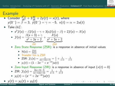
ExampleI Consider d2y
dt2 + 3dydt + 2y(t) = x(t), where
y(0−) = β = 3, y(0−) = γ = −5, x(t) = α = 2u(t)I Take UL:
I s2Y(s)− βY(s)− γ + 3(sY(s)− β) + 2Y(s) = X (s)
I Y(s) =β(s + 3) + γ
s2 + 3s + 2︸ ︷︷ ︸ZIR
+X (s)
s2 + 3s + 2︸ ︷︷ ︸ZSR
I Zero State Response (ZSR): is a response in absence of initial values
I H(s) = Y(s)X (s)
I Transfer fcn is ZSRI ZSR: Y1(s) = α
s(s+1)(s+2)= 1
s+ 1
s+2− 2
s+1
I y1(t) = (1− 2e−t + e−2t)u(t)
I Zero Input Response (ZIR): is a response in absence of input (x(t) = 0)I ZIR: Y2(s) = 3(s+3)−5
(s+1)(s+2) = 1s+1 + 2
s+2
I y2(t) = (e−t + 2e−2t)u(t)
I y(t) = y1(t) + y2(t)Farzaneh Abdollahi Signal and Systems Lecture 7 31/48
Outline Introduction Analyzing LTI Systems with LT Geometric Evaluation Unilateral LT Feed Back Applications State Space Representation
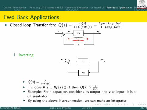
Feed Back ApplicationsI Closed loop Transfer fcn: Q(s) = G(s)
1+G(s)H(s) = Open loop Gain1−Loop Gain
1. Inverting
I Q(s) = K1+Kp(s)
I If choose K s.t. Kp(s)� 1 then Q(s) ' 1p(s)
I Example: For a capacitor, consider i as output and v as input, it is adifferentiator
I By using the above interconnection, we can make an integrator
Farzaneh Abdollahi Signal and Systems Lecture 7 32/48
Outline Introduction Analyzing LTI Systems with LT Geometric Evaluation Unilateral LT Feed Back Applications State Space Representation
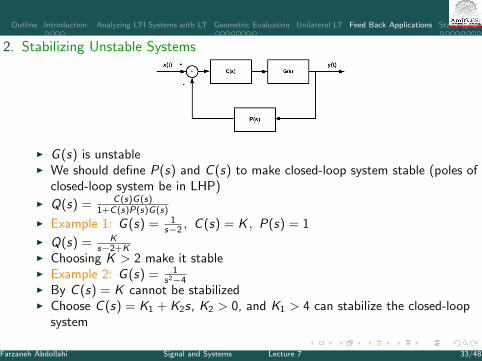
2. Stabilizing Unstable Systems
I G (s) is unstableI We should define P(s) and C (s) to make closed-loop system stable (poles of
closed-loop system be in LHP)I Q(s) = C(s)G(s)
1+C(s)P(s)G(s)
I Example 1: G (s) = 1s−2 , C (s) = K , P(s) = 1
I Q(s) = Ks−2+K
I Choosing K > 2 make it stableI Example 2: G (s) = 1
s2−4I By C (s) = K cannot be stabilizedI Choose C (s) = K1 + K2s, K2 > 0, and K1 > 4 can stabilize the closed-loop
system
Farzaneh Abdollahi Signal and Systems Lecture 7 33/48
Outline Introduction Analyzing LTI Systems with LT Geometric Evaluation Unilateral LT Feed Back Applications State Space Representation
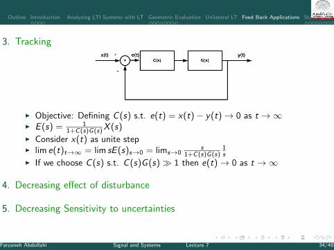
3. Tracking
I Objective: Defining C (s) s.t. e(t) = x(t)− y(t)→ 0 as t →∞I E (s) = 1
1+C(s)G(s)X (s)I Consider x(t) as unite stepI lim e(t)t→∞ = lim sE (s)s→0 = lims→0
s1+C(s)G(s)
1s
I If we choose C (s) s.t. C (s)G (s)� 1 then e(t)→ 0 as t →∞
4. Decreasing effect of disturbance
5. Decreasing Sensitivity to uncertainties
Farzaneh Abdollahi Signal and Systems Lecture 7 34/48
Outline Introduction Analyzing LTI Systems with LT Geometric Evaluation Unilateral LT Feed Back Applications State Space Representation
State Space Representation
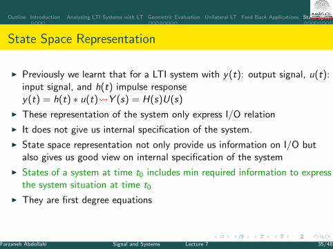
I Previously we learnt that for a LTI system with y(t): output signal, u(t):input signal, and h(t) impulse responsey(t) = h(t) ∗ u(t) Y (s) = H(s)U(s)
I These representation of the system only express I/O relation
I It does not give us internal specification of the system.
I State space representation not only provide us information on I/O butalso gives us good view on internal specification of the system
I States of a system at time t0 includes min required information to expressthe system situation at time t0
I They are first degree equations
Farzaneh Abdollahi Signal and Systems Lecture 7 35/48
Outline Introduction Analyzing LTI Systems with LT Geometric Evaluation Unilateral LT Feed Back Applications State Space Representation
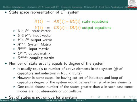
I State space representation of LTI system
X (t) = AX (t) + BU(t) state equations
Y (t) = CX (t) + DU(t) output equationsI X ∈ Rn: state vectorI U ∈ Rm: input vectorI Y ∈ Rp output vectorI An×n: System MatrixI Bn×m: input matrixI C p×n: output matrixI Dp×m: coupling matrix
I Number of state usually equals to degree of the systemI It usually equals to number of active elements in the system (# of
capacitors and inductors in RLC circuits)I However in some cases like having cut-set of inductors and loop of
capacitors degree of the system would be less than # of active elementsI One could choose number of the states greater than n in such case some
modes are not observable or controllable
I Set of states is not unique for a systemFarzaneh Abdollahi Signal and Systems Lecture 7 36/48
Outline Introduction Analyzing LTI Systems with LT Geometric Evaluation Unilateral LT Feed Back Applications State Space Representation
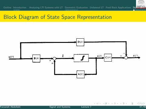
Block Diagram of State Space Representation
Farzaneh Abdollahi Signal and Systems Lecture 7 37/48
Outline Introduction Analyzing LTI Systems with LT Geometric Evaluation Unilateral LT Feed Back Applications State Space Representation
Solving State Equations by UL
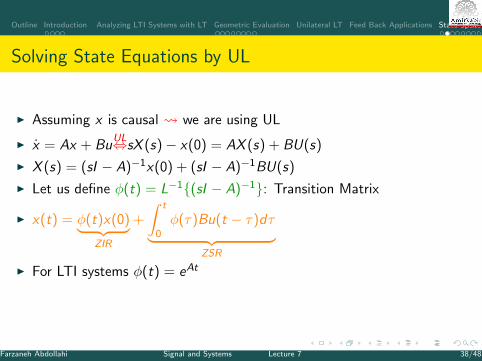
I Assuming x is causal we are using UL
I x = Ax + BuUL⇔sX (s)− x(0) = AX (s) + BU(s)
I X (s) = (sI − A)−1x(0) + (sI − A)−1BU(s)
I Let us define φ(t) = L−1{(sI − A)−1}: Transition Matrix
I x(t) = φ(t)x(0)︸ ︷︷ ︸ZIR
+
∫ t
0φ(τ)Bu(t − τ)dτ︸ ︷︷ ︸
ZSR
I For LTI systems φ(t) = eAt
Farzaneh Abdollahi Signal and Systems Lecture 7 38/48
Outline Introduction Analyzing LTI Systems with LT Geometric Evaluation Unilateral LT Feed Back Applications State Space Representation
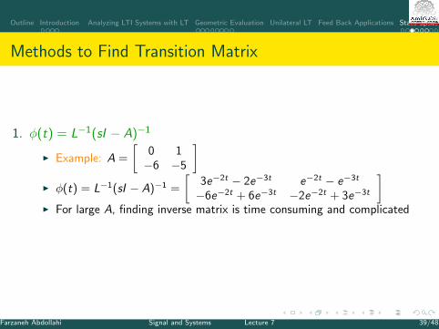
Methods to Find Transition Matrix
1. φ(t) = L−1(sI − A)−1
I Example: A =
[0 1−6 −5
]I φ(t) = L−1(sI − A)−1 =
[3e−2t − 2e−3t e−2t − e−3t
−6e−2t + 6e−3t −2e−2t + 3e−3t
]I For large A, finding inverse matrix is time consuming and complicated
Farzaneh Abdollahi Signal and Systems Lecture 7 39/48
Outline Introduction Analyzing LTI Systems with LT Geometric Evaluation Unilateral LT Feed Back Applications State Space Representation
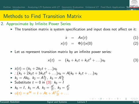
Methods to Find Transition Matrix
2. Approximate by Infinite Power SeriesI The transition matrix is system specification and input does not affect on it:
x = Ax(t) (1)
x(t) = Φ(t)x(0) (2)
I Let us represent transition matrix by an infinite power series:
x(t) = (k0 + k1t + k2t2 + . . .)x0 (3)
I x(t) = (k1 + 2k2t + . . .)x0
I ∴(k1 + 2k2t + 3k3t2 + . . .)x0 = A(k0 + k1t + . . .)x0
I k1 = Ak0, k2 = A k1
2 , k3 = A k2
3I Substitute t = 0 in (3): k0 = II k0 = I , k1 = A, k2 = A2
2! , k3 = A3
3!
I φ(t) = eAt = I + At + A2 t2
2! + . . .
Farzaneh Abdollahi Signal and Systems Lecture 7 40/48
Outline Introduction Analyzing LTI Systems with LT Geometric Evaluation Unilateral LT Feed Back Applications State Space Representation
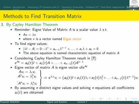
Methods to Find Transition Matrix
3. By Cayley Hamilton TheoremI Reminder: Eigne Value of Matrix A is a scalar value λ s.t.
I Av = λvI where v is a vector named Eigne vector
I To find eigne values:I |λI − A| = 0 λn + an−1λ
n−1 + . . .+ a1λ+ a0 = 0I The above equation is named characteristic equation of matrix A
I Considering Cayley Hamilton Theorem result in [?]:eAt = a0(t)I + a1(t)A + . . .+ an−1(t)An−1
I Eigne vector of matrix A is eigne vector ofeAt
Avi = λiviA2vi = λ2
i vi...Anvi = λni vi
⇒ eλi tvi = (a0(t)I+a1(t)λi +a2(t)λ2i +. . .+an−1(t)λn−1)vi
I By assuming n distinct eigne values and solving n equations all coefficientsai (t) are obtained
Farzaneh Abdollahi Signal and Systems Lecture 7 41/48
Outline Introduction Analyzing LTI Systems with LT Geometric Evaluation Unilateral LT Feed Back Applications State Space Representation
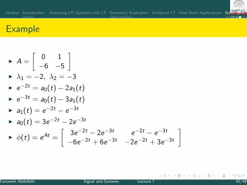
Example
I A =
[0 1−6 −5
]I λ1 = −2, λ2 = −3
I e−2t = a0(t)− 2a1(t)
I e−3t = a0(t)− 3a1(t)
I a1(t) = e−2t − e−3t
I a0(t) = 3e−2t − 2e−3t
I φ(t) = eAt =
[3e−2t − 2e−3t e−2t − e−3t
−6e−2t + 6e−3t −2e−2t + 3e−3t
]
Farzaneh Abdollahi Signal and Systems Lecture 7 42/48
Outline Introduction Analyzing LTI Systems with LT Geometric Evaluation Unilateral LT Feed Back Applications State Space Representation
Defining Transfer Function from State Space Eq.
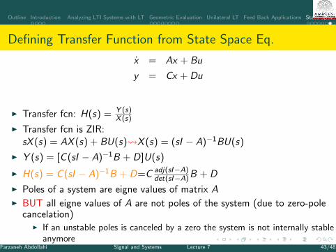
x = Ax + Bu
y = Cx + Du
I Transfer fcn: H(s) = Y (s)X (s)
I Transfer fcn is ZIR:sX (s) = AX (s) + BU(s) X (s) = (sI − A)−1BU(s)
I Y (s) = [C (sI − A)−1B + D]U(s)
I H(s) = C (sI − A)−1B + D=C adj(sI−A)det(sI−A)B + D
I Poles of a system are eigne values of matrix AI BUT all eigne values of A are not poles of the system (due to zero-pole
cancelation)I If an unstable poles is canceled by a zero the system is not internally stable
anymoreFarzaneh Abdollahi Signal and Systems Lecture 7 43/48
Outline Introduction Analyzing LTI Systems with LT Geometric Evaluation Unilateral LT Feed Back Applications State Space Representation
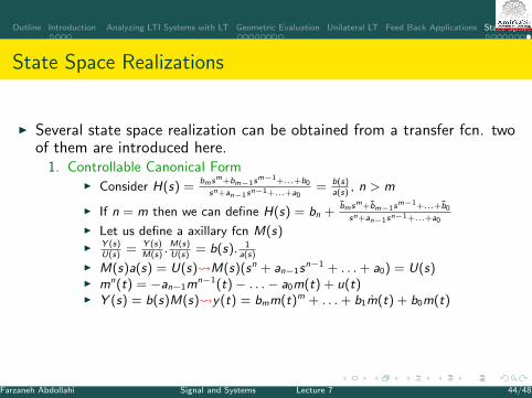
State Space Realizations
I Several state space realization can be obtained from a transfer fcn. twoof them are introduced here.
1. Controllable Canonical FormI Consider H(s) =
bmsm+bm−1sm−1+...+b0
sn+an−1sn−1+...+a0= b(s)
a(s), n > m
I If n = m then we can define H(s) = bn +bmsm+bm−1s
m−1+...+b0
sn+an−1sn−1+...+a0
I Let us define a axillary fcn M(s)I Y (s)
U(s)= Y (s)
M(s).M(s)U(s)
= b(s). 1a(s)
I M(s)a(s) = U(s) M(s)(sn + an−1sn−1 + . . .+ a0) = U(s)
I mn(t) = −an−1mn−1(t)− . . .− a0m(t) + u(t)
I Y (s) = b(s)M(s) y(t) = bmm(t)m + . . .+ b1m(t) + b0m(t)
Farzaneh Abdollahi Signal and Systems Lecture 7 44/48
Outline Introduction Analyzing LTI Systems with LT Geometric Evaluation Unilateral LT Feed Back Applications State Space Representation
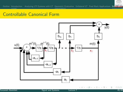
Controllable Canonical Form
Farzaneh Abdollahi Signal and Systems Lecture 7 45/48
Outline Introduction Analyzing LTI Systems with LT Geometric Evaluation Unilateral LT Feed Back Applications State Space Representation
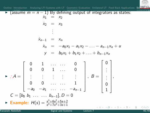
I (assume m = n − 1) By defining output of integrators as states:x1 = x2
x2 = x3
...
xn−1 = xn
xn = −a0x1 − a1x2 − . . .− an−1xn + u
y = b0x1 + b1x2 + . . .+ bn−1xn
I ∴A =
0 1 . . . . . . 00 0 1 . . . 0...
......
......
0 0 . . . . . . 1−a0 −a1 . . . . . . −an−1
, B =
0......01
,
C = [b0 b1 . . . . . . bn−1],D = 0
I Example: H(s) = s3+6s2+5s+2s3+7s2+3s+1
Farzaneh Abdollahi Signal and Systems Lecture 7 46/48
Outline Introduction Analyzing LTI Systems with LT Geometric Evaluation Unilateral LT Feed Back Applications State Space Representation
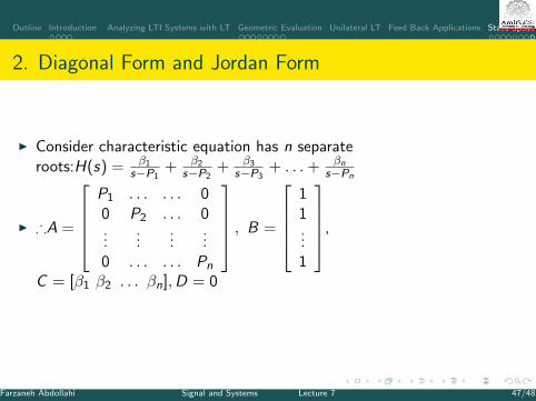
2. Diagonal Form and Jordan Form
I Consider characteristic equation has n separateroots:H(s) = β1
s−P1+ β2
s−P2+ β3
s−P3+ . . .+ βn
s−Pn
I ∴A =
P1 . . . . . . 00 P2 . . . 0...
......
...0 . . . . . . Pn
, B =
11...1
,
C = [β1 β2 . . . βn],D = 0
Farzaneh Abdollahi Signal and Systems Lecture 7 47/48
Outline Introduction Analyzing LTI Systems with LT Geometric Evaluation Unilateral LT Feed Back Applications State Space Representation
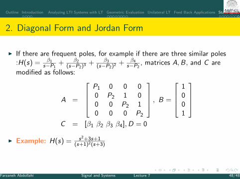
2. Diagonal Form and Jordan Form
I If there are frequent poles, for example if there are three similar poles:H(s) = β1
s−P1+ β2
(s−P2)3 + β3
(s−P2)2 + β4s−P2
, matrices A,B, and C are
modified as follows:
A =
P1 0 0 00 P2 1 00 0 P2 10 0 0 P2
, B =
1001
C = [β1 β2 β3 β4],D = 0
I Example: H(s) = s2+3s+1(s+1)2(s+3)
Farzaneh Abdollahi Signal and Systems Lecture 7 48/48