SIGNALS AND SYSTEMS LABORATORY - …site.iugaza.edu.ps/mbohisi/files/2016/09/Experiment-5.pdf ·...

Islamic University Of Gaza

Faculty of Engineering

Electrical Engineering department

SIGNALS AND SYSTEMS

LABORATORY

Signals And Systems Lab EELE (3110)

Page 1 of 21

Experiments #5

Signal generation system using LabView & MatLab

1) Introduction:

In signals and systems lab, (M-File) coding is widely used specially by using MatLab program, but there is new program called LabView program with its module called MathScript can also use to writing (M-File) coding.

MathScript is a feature of the newer versions of LabView that allows one to include M-File within its graphical environment. As a result, one can perform hybrid programming, that is, a combination of textual and graphical programming, when using this feature.

This lab provides an introduction to MathScript or M-File textual coding.

The MathScript is an interactive window or node on the LabView which shown in Figure 5.1, consists of a Command Window, an Output Window and a MathScript Window.

The Command Window interface allows one to enter commands and debug script or

to view help statements for built-in functions.

The Output Window is used to view output values.

The MathScript Window interface to display variables and command history as well

as edit scripts, with script editing, one can execute a group of commands or textual

statements.

Note:

- The MathScript has the same commands and functions which the MatLab has.

- Back to experiments 1&2 and execute its commands and functions by using

MathScript window. - To show the MathScript window open new VI and press (Ctrl-E) to open a block

diagram window then choose (Tools MathScript window).


Page 2 of 21

A LabView MathScript node represents the textual M-File code via a blue rectangle as shown

in Figure 5.2, its inputs and outputs are defined on the border of this rectangle for transferring

data between the graphical environment and the textual code.

For example, as indicated in Figure 5.2, the input variables on the left side, namely X and Y

transfer values to the M-File script, and the output variables on the right side, Sum and

Average, transfer values to the graphical environment, this process allows M-File script

variables to be used within the LabView graphical programming environment.

Figure 5.1: LabView MathScript Interactive window

Output Window MathScript Window

Command Window


Page 3 of 21

Figure 5.2: The MathScript node Interface

2) LabView MathScript and Hybrid Programming:

Back to the functions and operations code in experiments one & two, these code we can use it in MathScript node as using in MatLab.

The LabView MathScript feature can be used to perform hybrid programming, in other words, a combination of textual M-Files and graphical objects. Normally, it is easier to carry out math operations via M-files while maintaining user interfacing, interactivity and analysis in the more intuitive graphical environment of LabView. Textual M-File codes can be typed in or copied and pasted into LabView MathScript nodes.

2.1) Find the Sum and Average Using Hybrid Programming:

In this example we will be compute the sum and the average for two input numeric numbers, adding MathScript into block diagram by right clicking (programming structures MathScript) to create MathScript node.

The inputs to this program consist of x and y, to add these inputs, right-click on the left border of the MathScript node and choose the Add Input option as shown in figure 5.3.


Page 4 of 21

Figure 5.3: Adding input and creating numeric control

After adding these inputs, create controls to change the inputs interactively via the front panel, by right-clicking on the right border choose add outputs option and select undetected. An important issue to consider is the selection of output data type, the outputs of the Sum and Average VI are scalar quantities, choose data types by right- clicking on an output and selecting the choose Data Type option, finally, add numeric indicator into front panel see figure 5.4 to show the complete program.

Figure 5.4: complete front panel and complete block diagram


Page 5 of 21

2.2) Building a Signal Generation System:

In this part of experiment we will try to generate a signal by using two different program LabView and MatLab which have common issue which is Textual M-File codes.

There are a very important signals called (useful signals), which are Step, Ramp and Impulse function so we can write an expression for any signal as linear combination of these useful signals, after defined its expression.

To be able to write its expression we need first to know their mathematical definition

1) Unit Step Function:

( ) = { 0 , < 0

1 , ≥ 0

2) Ramp Function:

( ) = {0 , < 0

, ≥ 0

3) Unit Impulse Function:

( ) = {0 , ≠ 0

, = 0


Page 6 of 21

BY MatLab Program:

Now, we will be write the definition of these signals using M-File function type which discussed in experiment #2 and save them with their names to be able to recall them.

For simulation purposes, a representation of time (t) is needed, note that the time scale is continuous while computer programs operate in a discrete fashion, this simulation can be achieved by considering a very small time interval.

For example, if a 1-second duration signal in millisecond increments (time interval of 0.001 second) is considered, then one sample every 1 millisecond and a total of 1000 samples are generated for the entire signal.

It is important to note that there is a finite number of samples for a continuous-time signal, and, to differentiate this signal from a discrete-time signal, one must assign a much higher number of samples per second (very small time interval).

1) Unit Step Function:

Open new M-File to write the expression of Unit-Step function as a function in MatLab as shown in figure 5.5.

Figure 5.5: Textual M-file code for Unit step function

We can represent the unit-step function by using command (hardlim (t)) in the command window or M-File.


Page 7 of 21

2) Ramp Function:

Open new M-File to write the expression of Ramp function as a function in MatLab as shown in figure 5.6.

Figure 5.6: Textual M-file code for Ramp function

We can represent the unit-step function by using command (poslin (t)) in the command window or M-File.

3) Unit Impulse Function:

Open new M-File to write the expression of Unit-Impulse function as a function in MatLab as shown in figure 5.7.


Page 8 of 21

Figure 5.7: Textual M-file code for Unit Impulse function

We can represent the Impulse function by using the same definition of Unit-Impulse function but divide the amplitude on delta (d = (1/delta)*…).

Now, we will test these expression and show the output from each one then test the properties of signals (shift, inversion, scaling) on these functions and plot the output.

- Examples: - Sketch the unit step function u(t) and shift it to right by one:

Figure 5.8: Textual M-File code for unit step function U(t)


Page 9 of 21

Unit-Step Function

1.5

1

0.5

0

-0.5 -2 -1.5 -1 -0.5 0

Time

0.5 1 1.5 2

Shifted Unit-Step Function

1.5

1

0.5

0

-0.5 -2 -1.5 -1 -0.5 0 0.5

Time

1 1.5 2 2.5 3

Figure 5.9: The output signal for U(t)

Figure 5.10: Textual M-File code for unit step function U(t-1)

Figure 5.11: The output signal for U(t-1)

Am

plit

ud

e

Am

plit

ude

of 21


- Sketch the following signal using MatLab program:

Figure 5.12: Textual M-File code for the Upper signal

Figure 5.13: The output signal for y (t)

Given Signal

1.5

1

0.5

0

-0.5 -2 -1.5 -1 -0.5 0

Time

0.5 1 1.5 2

Am

plit

ude

of 21


- Sketch the following signal using MatLab program:

Figure 5.14: Textual M-File code for the Upper signal

of 21


Given Signal

4

3.5

3

2.5

2

1.5

1

0.5

0

-0.5

-2 0 2 4

Time

6 8 10

Figure 5.15: The output signal for y (t)

BY LabView Program:

As we say before we can use the LabView program to write M-File code and execute it using hybrid program techniques, by using an extension Module called MathScript Module (install it as you install the LabView).

As we said before the MathScript has two types (window, node), now we will be use the two type to write the mathematical definition for useful function which shown before.

Let we see how we can write the mathematical definition for useful function

- First we need to define these function using MathScript window and write the M- File code for each function and save it is specific folder to be call it and any time by its name.

- So, let we start by Unit-step function and write its textual M-File code after we open the MathScript window and create a new Script file which will be start by function word to be a Function in LabView.

Am

plit

ude

of 21


1) Unit-Step Function:

Open a new Blank VI file and go to block diagram then select (Tools MathScript window) and wait until initializing finish then select script icon.

Now, start the M-file by word “Function” to be function file, then write the standard form of Function as shown in figure 5.16.

Figure 5.16: Textual M-File code for Unit-Step function

There a very important step which is determine the path of folder that contain the M- files for functions to be able to call the function at any time by its name, so to do that you need to make the following instructions:

- Save the M-file of the function at any folder or location and keep its path in your

mind.

- Then select (File LabView MathScript properties) or press (Ctrl+I) then

select (MathScript: search paths).

- Then press on the first icon to add folder.

- Then open the path of the folder which content the M-File of functions and press

on (current folder) icon.

- Then press on (Apply and save) icon.

- Now, we can call any function on MathScript window or node from this folder.

- You can make another path to save on it as the previous steps.

of 21


Figure 5.17: LabView MathScript properties dialog window

2) Ramp Function:

Open a new script file by press on (New Script) icon, then start this file by Function word to be function M-file and then write the mathematical definition for Ramp function as shown in Figure 5.18.

Figure 5.18: Textual M-File code for Ramp Function

Note:

When you to save the script file select (File save script as) to correctly save, because if you press on the save icon in the ribbon bar the new file will be save on the old one.

of 21


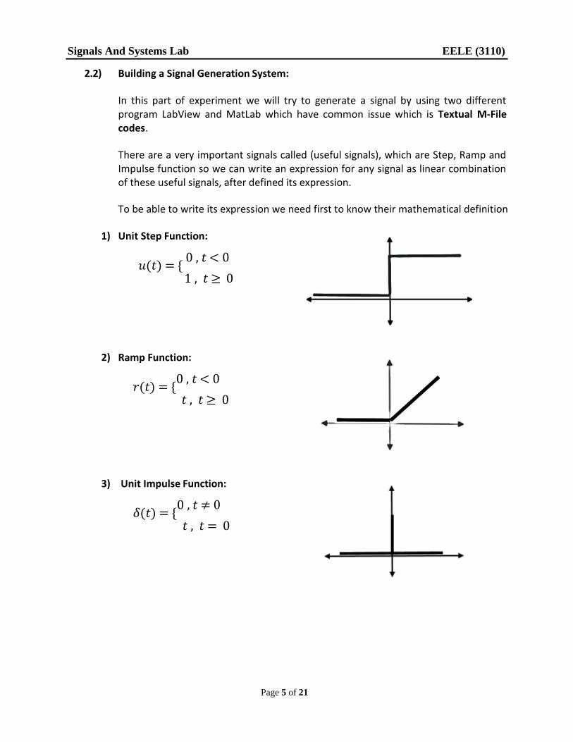
3) Unit-Impulse Function:

Open a new script file by press on (New Script) icon, then start this file by Function word to be function M-file and then write the mathematical definition for unit- Impulse function which is construct from linear combination of unit step function as shown in figure 5.19.

Figure 5.19: Textual M-File code for Unit-Impulse function

We can represent the Impulse function by using the same definition of Unit-Impulse function but divide the amplitude on delta (d = (1/delta)*…).

Now, we will test these expression and show the output from each one then test the properties of signals (shift, inversion, scaling) on these functions and plot the output.

- Example: - Sketch the following signal using MathScript window:

First by using MathScript window:

of 21


Figure 5.20: Textual M-file code for the upper signal

Figure 5.21: The output signal which match the upper one

of 21


Second way by using another type MathScript Node:

Open a new blank VI and go to block diagram window by press (Ctrl-E) then right clicking on white area to open function palette (programming structures MathScript Node) then determine the specific area you want and add its as you add while loop and for loop.

As we said before the right boundary is input wall and the left boundary is output wall so, you can create an input or an output on these walls by right click on it and choose add input the write its name inside the rectangular which appear on the wall.

Now, let we see how we can use the graphical interface environment and the MathScript code together to make hybrid program.

Note that you can called the function from this node and use the same code which use in the previous example (Ctrl-C & Ctrl-V) on the MathScript node but here we will be use the graphical interface to input value of dt and display the output on oscilloscope without plot command as shown in figure 5.22.

Figure 5.22: The block diagram for the VI that plot the upper signals

Figure 5.23: The front panel for VI that plot the upper signals

of 21


In the previous example we use a new waveform graph that called (Express XY graph) to sketch the relation between the two values which are (Time & Amplitude) where time variable (t) we defined in M-File code not the real time in LabView, so if you try to use waveform graph with the same definition for t it will be consider as time shift because the time axis in waveform graph always start from zero, that mean there is no negative value in its axis.

If you try to turn off the automatic scale in the waveform graph for x-axis (time) the signal will be start from zero, if you want to use this type of an indicator you should be defined the time variable to start from zero another case the signal will be shift by the value in negative.

An example on the previous notes, if you defined a variable t as start from -2 so the signal will be shift to right by 2 as shown in figure 5.24.

Explain: if we consider the variable t has this interval (t=-2:0.001:2) so the waveform graph consider t as (t=0:0.001:4).

Figure 5.24: display signal using waveform graph

As you see the time axis divide from (0 to 6000), so now you ask yourself from where it’s come, the answer we say before now in the previous example which is sketch the two signal we defined t from -1:0.001:5 so your rang length equal 6 and the increment dt=0.001 that mean you have 1000 sample/sec (1/dt) and the length equal 6 sec, so you have in this range 6000 samples (1000*6) that equal the total samples.

of 21


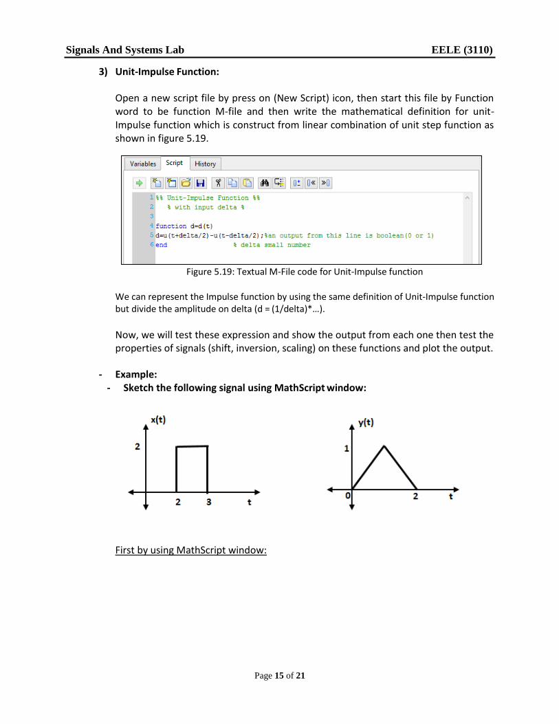
- Building a Periodic Signal Generation System Using Hybrid Programming:

This system involves generating a periodic signal in textual mode and displaying it in graphical mode, modify the shape of the signal (sine, square, triangle or sawtooth) as well as its frequency and amplitude by using appropriate front panel controls.

The block diagram and front panel of this system using a LabView MathScript node are shown in Figure 5.25 and Figure 5.26, respectively.

The front panel includes the following three controls:

- Waveform type: Select the shape of the input waveform as either sine, square, triangular or sawtooth waves.

- Amplitude: Control the amplitude of the input waveform. - Frequency: Control the frequency of the input waveform.

To build the front panel interface as shown in figure5.26, add two Knob one for amplitude and another for frequency, then choose (Text ring) from text control library to select the type of signal generated.

Now, how we can enter the data in this icon by right clicking on it and choose (properties Edit Items Insert) then insert the item like (sin, square, …….) and give each item value as (0, 1 ,2 ,…..) as shown in the figure 5.27.

Figure 5.27: The properties dialog window for ring control

of 21


Figure 5.26: The front panel for signal generation system

Figure 5.25: the block diagram for signal generation system

The new function is called build waveform and it has two input (y, dt) and the output is the graph of output signal with it increment value.

of 21


Exercises:

1) Sketch a signal x(t) which has the following expression by using MatLab program:

( ) = {

0 , < 0 2 , 0 ≤ < 1

2 − +1, ≥ 1

And answer into the following question:

a. Find the even part of this function and sketch it. b. Find the odd part of this function and sketch it. c. Then verify if (original signal= even + odd signal) satisfy or not.

2) Design a different type of filters (Low pass, Band pass, High pass) with varying parameter using MathScript node, and I want to be able to change these parameter (t0, t1) and choose the filter type from front panel.

Note: to test your program use sinusoidal signal with time interval (0 to 4π)

Figure 5.28: An illustration graph for the upper exercise

SIGNALS AND SYSTEMS LABORATORY - …site.iugaza.edu.ps/mbohisi/files/2016/09/Experiment-5.pdf ·...

Documents

Transcript of SIGNALS AND SYSTEMS LABORATORY - …site.iugaza.edu.ps/mbohisi/files/2016/09/Experiment-5.pdf ·...