Signal Processing of FMCW Synthetic Aperture Radar...

“prova˙tesi” — 2006/8/20 — 21:49 — page i — #1�

�

�

�

�

�

�

�

Signal Processing of FMCW Synthetic Aperture

Radar Data

“prova˙tesi” — 2006/8/20 — 21:49 — page ii — #2�

�

�

�

�

�

�

�

The pictures on the cover are FMCW SAR images produced with and withoutusing the range frequency non-linearity correction algorithm developed by theauthor. (See also figure 7.11 of this thesis).

“prova˙tesi” — 2006/8/20 — 21:49 — page iii — #3�

�

�

�

�

�

�

�

Signal Processing of FMCW Synthetic Aperture

Radar Data

Proefschrift

ter verkrijging van de graad van doctoraan de Technische Universiteit Delft,

op gezag van de Rector Magnificus prof.dr.ir. J.T. Fokkema,voorzitter van het College voor Promoties,

in het openbaar te verdedigen op maandag 2 oktober 2006 om 15:00 uur

door

Adriano METALaurea di dottore in Ingegneria delle Telecomunicazioni

Universita’ degli Studi di Roma “La Sapienza”

geboren te Pontecorvo, Italie.

“prova˙tesi” — 2006/8/20 — 21:49 — page iv — #4�

�

�

�

�

�

�

�

Dit proefschrift is goedgekeurd door de promotor:Prof.ir. P. HoogeboomProf.dr.ir. L.P. Ligthart

Samenstelling promotiecomissie:

Rector Magnificus, voorzitterProf.ir. P. Hoogeboom Technische Universiteit Delft, promotorProf.dr.ir. L.P. Ligthart, Technische Universiteit Delft, promotorProf.dr. C. Baker, University College LondonProf.dr. A. Moreira, DLR Institut fur Hochfrequenztechnik und RadarsystemeProf.dr. S. Vassiliadis, Technische Universiteit DelftDr.ir. R.F. Hanssen, Technische Universiteit DelftDrs. W. Pelt, Ministerie van Defensie

This research was supported by the Dutch Technology Foundation STW, applied sciencedivision NWO and the technology programme of the Ministry of Economic Affairs. Theproject was granted under number DTC.5642.The work was furthermore supported by TNO Defence, Security and Safety.

ISBN 907692810XSignal Processing of FMCW Synthetic Aperture Radar Data.Dissertation at Delft University of Technology.Copyright c© 2006 by A. Meta.

All rights reserved. No parts of this publication may be reproduced or transmitted in anyform or by any means, electronic or mechanical, including photocopy, recording, or anyinformation storage and retrieval system, without permission in writing from the author.

“prova˙tesi” — 2006/8/20 — 21:49 — page v — #5�

�

�

�

�

�

�

�

to our little Andrea

“prova˙tesi” — 2006/8/20 — 21:49 — page vi — #6�

�

�

�

�

�

�

�

“prova˙tesi” — 2006/8/20 — 21:49 — page vii — #7�

�

�

�

�

�

�

�

CONTENTS vii

Contents

1 Introduction 11.1 Research motivation . . . . . . . . . . . . . . . . . . . . . . . . . . . . . . . 21.2 Research objectives . . . . . . . . . . . . . . . . . . . . . . . . . . . . . . . 21.3 Novelties and main results . . . . . . . . . . . . . . . . . . . . . . . . . . . 31.4 Outline of the thesis . . . . . . . . . . . . . . . . . . . . . . . . . . . . . . . 4References . . . . . . . . . . . . . . . . . . . . . . . . . . . . . . . . . . . . . . . 5

2 FMCW radar and SAR overview 72.1 The FMCW radar principle . . . . . . . . . . . . . . . . . . . . . . . . . . . 72.2 The Synthetic Aperture Radar principle . . . . . . . . . . . . . . . . . . . . 9

2.2.1 Range migration . . . . . . . . . . . . . . . . . . . . . . . . . . . . 102.2.2 Motion errors . . . . . . . . . . . . . . . . . . . . . . . . . . . . . . 10

References . . . . . . . . . . . . . . . . . . . . . . . . . . . . . . . . . . . . . . . 11

3 Range processing in FMCW 133.1 Introduction . . . . . . . . . . . . . . . . . . . . . . . . . . . . . . . . . . . 133.2 Linear deramped FMCW signals . . . . . . . . . . . . . . . . . . . . . . . . 14

3.2.1 Stationary targets . . . . . . . . . . . . . . . . . . . . . . . . . . . . 153.2.2 Moving targets . . . . . . . . . . . . . . . . . . . . . . . . . . . . . 16

3.3 Non-linearities in FMCW signals . . . . . . . . . . . . . . . . . . . . . . . . 163.4 Non-linearity correction . . . . . . . . . . . . . . . . . . . . . . . . . . . . . 17

3.4.1 Algorithm overview . . . . . . . . . . . . . . . . . . . . . . . . . . 193.4.2 Analytical development . . . . . . . . . . . . . . . . . . . . . . . . 213.4.3 Simulation . . . . . . . . . . . . . . . . . . . . . . . . . . . . . . . 223.4.4 Frequency non-linearity estimation . . . . . . . . . . . . . . . . . . 24

3.5 Linear SFCW signal . . . . . . . . . . . . . . . . . . . . . . . . . . . . . . 253.6 Randomized non-linear SFCW . . . . . . . . . . . . . . . . . . . . . . . . . 26

3.6.1 Non linear deramping technique . . . . . . . . . . . . . . . . . . . . 263.6.2 Stationary targets . . . . . . . . . . . . . . . . . . . . . . . . . . . . 283.6.3 Moving targets . . . . . . . . . . . . . . . . . . . . . . . . . . . . . 293.6.4 Influence of hardware non ideality . . . . . . . . . . . . . . . . . . . 31

3.7 Summary . . . . . . . . . . . . . . . . . . . . . . . . . . . . . . . . . . . . 32

“prova˙tesi” — 2006/8/20 — 21:49 — page viii — #8�

�

�

�

�

�

�

�

viii CONTENTS

References . . . . . . . . . . . . . . . . . . . . . . . . . . . . . . . . . . . . . . . 33

4 Cross-range imaging with FMCW SAR 354.1 Introduction . . . . . . . . . . . . . . . . . . . . . . . . . . . . . . . . . . . 354.2 Signal processing aspects . . . . . . . . . . . . . . . . . . . . . . . . . . . . 364.3 Analytical development . . . . . . . . . . . . . . . . . . . . . . . . . . . . . 394.4 Stripmap FMCW SAR simulation . . . . . . . . . . . . . . . . . . . . . . . 404.5 Spotlight FMCW SAR . . . . . . . . . . . . . . . . . . . . . . . . . . . . . 414.6 Digital beam forming FMCW SAR . . . . . . . . . . . . . . . . . . . . . . . 424.7 Summary . . . . . . . . . . . . . . . . . . . . . . . . . . . . . . . . . . . . 46References . . . . . . . . . . . . . . . . . . . . . . . . . . . . . . . . . . . . . . . 46

5 Moving Targets and FMCW SAR 495.1 Introduction . . . . . . . . . . . . . . . . . . . . . . . . . . . . . . . . . . . 495.2 Moving target Doppler spectrum . . . . . . . . . . . . . . . . . . . . . . . . 505.3 MTI with linear triangular FMCW SAR . . . . . . . . . . . . . . . . . . . . 515.4 MTI with randomized non-linear SFCW SAR . . . . . . . . . . . . . . . . . 555.5 Summary . . . . . . . . . . . . . . . . . . . . . . . . . . . . . . . . . . . . 60References . . . . . . . . . . . . . . . . . . . . . . . . . . . . . . . . . . . . . . . 60

6 FMCW SAR demonstrator system 616.1 Introduction . . . . . . . . . . . . . . . . . . . . . . . . . . . . . . . . . . . 616.2 Front-end . . . . . . . . . . . . . . . . . . . . . . . . . . . . . . . . . . . . 62

6.2.1 Steering signal . . . . . . . . . . . . . . . . . . . . . . . . . . . . . 636.2.2 Predistorted linearization . . . . . . . . . . . . . . . . . . . . . . . . 63

6.3 Noise power calculation . . . . . . . . . . . . . . . . . . . . . . . . . . . . . 676.3.1 Thermal noise . . . . . . . . . . . . . . . . . . . . . . . . . . . . . . 686.3.2 Phase noise . . . . . . . . . . . . . . . . . . . . . . . . . . . . . . . 696.3.3 Quantization noise . . . . . . . . . . . . . . . . . . . . . . . . . . . 706.3.4 Total noise . . . . . . . . . . . . . . . . . . . . . . . . . . . . . . . 70

6.4 Experimental tests . . . . . . . . . . . . . . . . . . . . . . . . . . . . . . . . 706.4.1 Noise laboratory measurements . . . . . . . . . . . . . . . . . . . . 716.4.2 Phase measurements . . . . . . . . . . . . . . . . . . . . . . . . . . 71

6.5 Summary . . . . . . . . . . . . . . . . . . . . . . . . . . . . . . . . . . . . 71References . . . . . . . . . . . . . . . . . . . . . . . . . . . . . . . . . . . . . . . 72

7 Flight test campaign results 737.1 Introduction . . . . . . . . . . . . . . . . . . . . . . . . . . . . . . . . . . . 737.2 Overview of the flight campaign . . . . . . . . . . . . . . . . . . . . . . . . 747.3 Non-linearities correction . . . . . . . . . . . . . . . . . . . . . . . . . . . . 78

7.3.1 First example . . . . . . . . . . . . . . . . . . . . . . . . . . . . . . 787.3.2 Second example . . . . . . . . . . . . . . . . . . . . . . . . . . . . 817.3.3 Third example . . . . . . . . . . . . . . . . . . . . . . . . . . . . . 83

“prova˙tesi” — 2006/8/20 — 21:49 — page ix — #9�

�

�

�

�

�

�

�

CONTENTS ix

7.4 High resolution images . . . . . . . . . . . . . . . . . . . . . . . . . . . . . 857.5 Medium resolution images . . . . . . . . . . . . . . . . . . . . . . . . . . . 877.6 Low resolution image . . . . . . . . . . . . . . . . . . . . . . . . . . . . . . 907.7 Resolution comparison . . . . . . . . . . . . . . . . . . . . . . . . . . . . . 927.8 Triangular FMCW SAR test . . . . . . . . . . . . . . . . . . . . . . . . . . 957.9 Summary . . . . . . . . . . . . . . . . . . . . . . . . . . . . . . . . . . . . 98References . . . . . . . . . . . . . . . . . . . . . . . . . . . . . . . . . . . . . . . 98

8 Conclusions and discussion 998.1 Contributions of this research . . . . . . . . . . . . . . . . . . . . . . . . . . 998.2 Recommendations . . . . . . . . . . . . . . . . . . . . . . . . . . . . . . . . 1008.3 Related works at other institutes . . . . . . . . . . . . . . . . . . . . . . . . 101References . . . . . . . . . . . . . . . . . . . . . . . . . . . . . . . . . . . . . . . 101

A Non-linear Frequency Scaling Algorithm for FMCW SAR data 103A.1 Introduction . . . . . . . . . . . . . . . . . . . . . . . . . . . . . . . . . . . 103A.2 Deramped non-linear FMCW SAR signal . . . . . . . . . . . . . . . . . . . 104A.3 Frequency non-linearity, Doppler shift and range cell migration correction . . 106A.4 Summary . . . . . . . . . . . . . . . . . . . . . . . . . . . . . . . . . . . . 107References . . . . . . . . . . . . . . . . . . . . . . . . . . . . . . . . . . . . . . . 107

List of acronyms 109

List of symbols 111

Summary 115

Samenvatting 117

Author’s publications 119

Acknowledgements 121

About the author 123

“prova˙tesi” — 2006/8/20 — 21:49 — page x — #10�

�

�

�

�

�

�

�

x CONTENTS

“prova˙tesi” — 2006/8/20 — 21:49 — page 1 — #11�

�

�

�

�

�

�

�

1

Chapter 1

Introduction

In the field of airborne earth observation, there is special attention for compact, cost effective,high resolution imaging sensors. Such sensors are foreseen to play an important role insmall-scale remote sensing applications, such as the monitoring of dikes, watercourses, orhighways. Furthermore, such sensors are of military interest; reconnaissance tasks could beperformed with small unmanned aerial vehicles (UAVs), reducing in this way the risk forone’s own troops.

In order to be operated from small, even unmanned, aircrafts, such systems must consumelittle power and be small enough to fulfill the usually strict payload requirements. Moreover,to be of interest for the civil market, a reasonable cost is mandatory.

Radar-based sensors have advantages over optical systems in their all weather capabilityand in the possibility to operate through smoke and at night. However, radar sensors used forimaging purposes exhibit relative low resolution in the cross-range or azimuth dimension, andfurthermore it gets coarser with increasing distance due to the constant antenna beamwidth.This limitation is overcome by Synthetic Aperture Radar (SAR) techniques. Such techniqueshave already been successful employed in the field of radar earth observation by using co-herent pulse radars. However, pulse radar systems are usually very complex instruments, andneither low cost nor compact. The fact that they are quite expensive makes them less suitablefor low-cost, civil applications, while their bulkiness could prevent them from being chosenfor UAV or small aircraft solutions.

Frequency Modulated Continuous Wave (FMCW) radar systems are, instead, generallycompact and relatively cheap to purchase and to exploit. FMCW radars consume little powerand, due to the fact that they are continuously operating, they can transmit a modest power,which makes them very interesting for military applications. Consequently, FMCW radartechnology is of interest for both civil and military airborne earth observation applications,specially in combination with high resolution SAR techniques. The novel combination ofFMCW technology and SAR techniques leads to the development of a small, lightweight,and cost-effective high resolution imaging sensor.

“prova˙tesi” — 2006/8/20 — 21:49 — page 2 — #12�

�

�

�

�

�

�

�

2 Chapter 1 . Introduction

1.1 Research motivation

SAR techniques have been successfully applied in combination with coherent pulse radars.Also the concept of synthetic aperture with FMCW sensors has already been put forward inliterature, [1] [2], and some experimental systems have been described, [3] [4]. However,the practical feasibility of an airborne FMCW SAR was not evident; the experimental sensorsdescribed in literature were, in fact, radars mounted on rail supports operating in ground SARconfigurations and at short distances. These FMCW radars could perform measurements ineach position of the synthetic aperture and then be moved to the next one. As in conventionalpulse SAR systems, the stop-and-go approximation could be used; such an approximationassumes the radar platform stationary during the transmission of the electromagnetic pulseand the reception of the corresponding echo. The approximation is valid for conventionalpulse systems because the duration of the transmitted waveform is relatively short and, ofcourse, is also valid for ground FMCW SAR where the radar can be actually fixed in a pre-determined position while making the measurements. For airborne FMCW radars, however,the stop-and-go approximation can be not valid anymore because the platform is actuallymoving while continuously transmitting. A complete model for the deramped FMCW SARsignal derived without using the stop-and-go approximation was missing in the literature.

In addition to the particular signal aspects relative to the combination of FMCW tech-nology and SAR techniques, the use of FMCW radars for high resolution and long rangeapplications was not evident. In practical FMCW sensors, in fact, the presence of unwantednon-linearities in the frequency modulation severely degrades the radar performances forlarge distances. Again, proper processing methods to overcome such limitation due to fre-quency non-linearities were not available to the scientific community.

Therefore, the area of FMCW SAR airborne observation and related signal processingaspects was a very novel field of research. At the International Research Centre for Telecom-munications and Radar (IRCTR) of the Delft University of Technology, a project was initiatedto investigate the feasibility of FMCW SAR in the field of airborne earth observation and todevelop proper processing algorithms to fully exploit the capability of such sensors.

1.2 Research objectives

Following from the motivations previously discussed, the first main objective of the projectwas to develop special processing SAR algorithms which could take into account the peculiarcharacteristics of an FMCW sensor. The features of major interest were: the presence offrequency non-linearities in the transmitted waveform and the fact that the FMCW sensor iscontinuously transmitting. The non-linearities represent a difference between an ideal andactual system, while the continuous motion has to be faced even when using sensors withperformance close to the ideal. In the literature, some non-linearity correction algorithmswere available, however they work only for very limited range intervals and, furthermore,require a reference point in each interval. For larger distance applications, as in the casefor SAR, the use of these algorithms is not efficient neither robust. In FMCW SAR, the

“prova˙tesi” — 2006/8/20 — 21:49 — page 3 — #13�

�

�

�

�

�

�

�

1.3 Novelties and main results 3

fact that the radar is continuously transmitting while moving means that the stop-and-goapproximation used for the derivation of conventional SAR algorithms could not be anymorevalid. These aspects needed to be analyzed and solutions had to be provided.

The continuous transmission, on the other hand, can be used as an advantage in differentother applications, as Moving Target Indication (MTI). In fact, in FMCW sensors, the pulseduration is considerably longer than in pulse radars, and therefore a better range frequencyresolution is possible. The combination of this property and the possibility of using differentkind of modulations (linear and non-linear) was investigated to see whether some FMCWSAR properties could be used to enhance the indication of moving targets.

The other main objective of the project was to show the practicability of FMCW SARunder operational circumstances. Therefore, concurrently with the signal processing algo-rithms elaboration, the development of a fully operational airborne demonstrator system andan X-band radar front-end was started at the Delft University of Technology. A complete anddetailed sensor model was required in order to estimate and analyze the performances of thesystem during the operational mode. In addition, the demonstrator system had to prove thatan FMCW SAR sensor can indeed be operated in an efficient and cost effective manner froma very small airborne platform. The work for the initial requirements to the FMCW SARsystem, the acquisition design and the development of the controlling software has been doneby dr.ir. J.J.M. de Wit within the framework of the project [5]. This part will not be treated inthis thesis.

1.3 Novelties and main results

Corresponding to the objectives set by the research project, the following novelties and mainresults have been reached and are presented in this thesis:

• Non-linearity correction. The author has developed a very innovative processing solu-tion, which completely solves the problem of the presence of frequency non-linearitiesin FMCW SAR. It corrects for the non-linearity effects for the whole range profile inone step, and it allows perfect range focusing, independently of the looking angle. Theproposed method operates directly on the deramped data and it is very computationallyefficient (Chapter 3, Section 3.4).

• Deramping technique for non-linear Stepped Frequency Continuous Wave (SFCW)signals. An extension to non-linear continuous signals of the deramping technique,commonly used in linear FMCW sensors, has been developed. With the proposed ex-tension, the great reduction in terms of sampling requirements can be achieved alsowhen using non-linear waveforms, at the cost of increased computation (Chapter 3,Section 3.6.1).

• A complete FMCW SAR signal model. The author has derived a detailed analyticalmodel for the FMCW SAR signal in the two-dimensional frequency domain. Based

“prova˙tesi” — 2006/8/20 — 21:49 — page 4 — #14�

�

�

�

�

�

�

�

4 Chapter 1 . Introduction

on this model, proper algorithms are developed which guarantee the best performanceswhen processing FMCW SAR data (Chapter 4).

• MTI with slope diversity in linear FMCW SAR. The author has exploited the possibilityof using triangular modulation for MTI by producing two images, respectively withthe upslope and downslope part of the transmitted waveform. Based on the FMCWSAR signal model, interferometric techniques on the pair of images can be used tohelp distinguishing moving targets from stationary clutter (Chapter 5, Section 5.3).

• MTI with randomized SFCW SAR. Based on the non-linear deramping technique previ-ously proposed, the author has analyzed how randomized non-linear SFCW SAR canbe used for MTI purposes (Chapter 5, Section 5.4).

• Detailed system model. A complete model description of the X-band FMCW SARfront-end system developed at the IRCTR, Delft University of Technology, has beenprovided. The system has been extensively tested by the author together with P. Hakkartand W.F. van der Zwan through ground and laboratory measurements, the results show-ing very good consistency with the developed model (Chapter 6).

• First demonstration of an X-band FMCW SAR. A flight test campaign has been orga-nized during the last part of 2005. The results were very successful. The feasibility ofan operational cheap FMCW SAR under practical circumstances has been proved.

• High resolution FMCW SAR images. Thanks to the special algorithms developed,FMCW SAR images with 45 cm times 25 cm resolution (including windowing) havebeen obtained for the first time.

1.4 Outline of the thesis

The remaining of this thesis is divided in seven chapters: in the first four, the theory ofFMCW SAR is introduced. Subsequently, the experimental system built at the IRCTR isdescribed; the methods previously developed are validated by processing real FMCW SARdata collected during the flight test campaign organized in the last part of 2005. The thesis isorganized as follows:

Chapter 2 provides a short overview of the FMCW radar and SAR principles. It introducesaspects which are then more deeply analyzed and discussed in the subsequent chapters.

Chapter 3 deals with the range processing of FMCW data and presents a novel processingsolution, which completely solves the frequency non-linearity problem. It corrects forthe non-linearity effects for the whole range profile and Doppler spectrum in one step,it operates directly on the deramped data and it is very computationally efficient. Non-linear SFCW modulation is also treated in the chapter; a novel deramping techniqueextended to the case of non-linear signals is introduced. With the extended deramping

“prova˙tesi” — 2006/8/20 — 21:49 — page 5 — #15�

�

�

�

�

�

�

�

1.4 References 5

technique proposed here, a reduced sampling frequency as for the linear case can beused also for randomized SFCW signals, at the cost of increased computation.

Chapter 4 derives a complete analytical model of the FMCW SAR signal description in thetwo-dimensional frequency domain, starting from the deramped signal and without us-ing the stop-and-go approximation. The model is then applied to stripmap, spotlightand single transmitter/multiple receiver Digital Beam Forming (DBF) synthetic aper-ture operational modes. Specially in the last two cases, the effects of the motion duringthe transmission and reception of the pulse can become seriously degrading for theSAR image quality, if not compensated.

Chapter 5 exploits the peculiar characteristics of the complex FMCW SAR image for Mov-ing Target Indication purposes. Two MTI methods are proposed in the chapter. Thefirst is based on the frequency slope diversity in the transmitted modulation by usinglinear triangular FMCW SAR. The second makes use of the Doppler filtering propertiesof randomized SFCW modulations.

Chapter 6 describes the X-band radar front-end developed at the Delft University of Tech-nology. A detailed system model is provided in order to estimate and analyze theperformance of the demonstrator system. Laboratory and ground based measurementsshow very good consistency with the calculated values, validating the model descrip-tion.

Chapter 7 presents the results obtained from the FMCW SAR flight test campaign orga-nized during the last part of 2005. Thanks to the special algorithms which have beendeveloped during the research project and described in the previous chapters, FMCWSAR images with a measured resolution up to 45 cm times 25 cm (including window-ing) were obtained for the first time. Several tests performed during the flight campaign(imaging at different resolutions, varying the incident angle, MTI experiment) are re-ported and discussed.

Chapter 8 summarizes the main results of the study which have led to this thesis; addition-ally, it draws conclusions and gives some recommendations for future work. Finally,as a demonstration of the increasing interest in FMCW SAR from the scientific andindustry community, the chapter reports some related works started at other institutes.

References

[1] H. D. Griffiths, “Synthetic Aperture Processing for Full-Deramp Radar,” IEE ElectronicLetters, vol. 24, no. 7, pp. 371–373, Mar. 1988.

[2] M. Soumekh, “Airborne Synthetic Aperture Acoustic Imaging,” IEEE Trans. on ImageProcessing, vol. 6, no. 11, pp. 1545–1554, Nov. 1997.

“prova˙tesi” — 2006/8/20 — 21:49 — page 6 — #16�

�

�

�

�

�

�

�

6 REFERENCES

[3] G. Connan, H. D. Griffiths, P. V. Brennan, D. Renouard, E. Barthlmy, and R. Garello,“Experimental Imaging of Internal Waves by a mm-Wave Radar,” in Proc. MTS/IEEEOceans ’98, Nice, France, Sept. 1998, pp. 619–623.

[4] Y. Yamaguchi, “Synthetic Aperture FM-CW Radar Applied to the Detection of ObjectsBuried in Snowpack,” IEEE Trans. Geosci. Remote Sensing, vol. 32, no. 1, pp. 11–18,Jan. 1994.

[5] J. J. M. de Wit, Development of an Airborne Ka-Band FM-CW Synthetic Aperture Radar.Delft University of Technology, Ph. D. thesis, 2005.

“prova˙tesi” — 2006/8/20 — 21:49 — page 7 — #17�

�

�

�

�

�

�

�

7

Chapter 2

FMCW radar and SAR overview

The chapter provides a short overview of the FMCW radar and SAR principles; it introduces aspects

which are then deeply analyzed and discussed in the following of the thesis.

2.1 The FMCW radar principle

FMCW is a continuous wave (CW) radar which transmits a frequency modulated (FM) signal[1]. In linear FMCW radars, the used modulation is usually a sawtooth. The ramp is alsoknown as a chirp, fig. 2.1(a). Objects illuminated by the antenna beam scatter part of thetransmitted signal back to the radar, where a receiving antenna collects this energy. The timethe signal travels to an object, or target, at a distance r and comes back to the radar is givenby:

τ =2r

c(2.1)

where c is the speed of light. In a homodyne FMCW receiver, the received signal is mixedwith a replica of the transmitted waveform and low pass filtered. This process is usually calledstretching or deramping. The resulting output is called the beat (or intermediate frequency)signal. From fig. 2.1(b), it can be seen that the frequency of the beat signal is directly pro-portional to the target time delay, and hence to the distance. The beat frequency is expressedas:

fb =B

PRIτ (2.2)

where B is the transmitted bandwidth given by the frequency sweep and PRI is the pulserepetition interval. In order to compress the range response, a Fourier transform is performedon the beat signal (fig. 2.1(c)), making the signal content available in the frequency domain.The response of a single target is qualitatively shown in fig. 2.1(d). A practical resulting signalfrom an FMCW sensor is the superposition of different sinusoidal signals, corresponding tothe environment being illuminated by the radar waves. In this case, the sidelobes of a strongtarget response could cover the signal of a weaker scatterer. Windowing the signal before

“prova˙tesi” — 2006/8/20 — 21:49 — page 8 — #18�

�

�

�

�

�

�

�

8 Chapter 2 . FMCW radar and SAR overview

applying the Fourier transform can reduce the sidelobe level at the expense of a broadeningof the main lobe. If a target is moving while being illuminated by the radar, its radial velocity

Time

Am

plit

ude

(a) Amplitude plot of a chirp signal. Thefrequency is linearly increasing with time

Time

Fre

quen

cy

PRI

fb τB

(b) Frequency plot of the chirp signal. Thereceived signal (dashed) is a delay versionof the transmitted (solid)

Time

Am

plit

ude

(c) Beat signal representation in the timedomain. The signal frequency is propor-tional to the scatterer distance.

Frequency, Range

Am

plit

ude

(d) Beat signal representation in the fre-quency domain. The frequency axis can bedirectly associated with range.

Figure 2.1: Overview of the linear FMCW radar principle.

component causes an additional Doppler frequency shift superimposed on the beat frequencydue to the actual distance, leading to an invalid range measurement. The Doppler shift isgiven by:

fD =2vr

λ(2.3)

“prova˙tesi” — 2006/8/20 — 21:49 — page 9 — #19�

�

�

�

�

�

�

�

2.2 The Synthetic Aperture Radar principle 9

where vr is the velocity in the radial direction and λ is the wavelength of the transmittedsignal.

2.2 The Synthetic Aperture Radar principle

In conventional Real Aperture Radar (RAR) systems, the azimuth resolution deteriorates withincreasing distances due to the constant antenna beamwidth. The RAR azimuth resolutionδazRARis given as:

δazRAR ≈ θazR (2.4)

in which θaz is the azimuth 3-dB antenna beamwidth and R is the target distance. It canbe noticed that in RAR systems the azimuth resolution is range dependent. The antennabeamwidth is related to the antenna length laz by:

θaz ≈ λ

laz(2.5)

As can be seen from (2.4) and (2.5), the azimuth resolution improves as the antenna lengthincreases. In synthetic aperture radar a large antenna length is synthesized by making use ofthe motion of the radar platform [2]. The platform on which the SAR is mounted is usually anaircraft or satellite. In order to review the SAR principle we will use a stripmap configuration.Its geometry and the radar position relative to the ground is shown in fig. 2.2. A burst of pulses

Figure 2.2: Stripmap SAR geometry.

is transmitted by the side-looking antenna pointed to the ground and the backscattered powerof each pulse is collected. The SAR is a coherent system, which means it retains the amplitudeand phase of the responses at each position as the radar moves. Due to the radar platformmotion, a stationary target is seen from different angles, which determines a variation of theradial velocity between the radar and the target. The Doppler shift induced by the radialvelocity varies approximately linearly with time (at least for narrow beamwidth systems),

“prova˙tesi” — 2006/8/20 — 21:49 — page 10 — #20�

�

�

�

�

�

�

�

10 Chapter 2 . FMCW radar and SAR overview

therefore the collected target response exhibits a Doppler bandwidth which is determined bythe variation of the angle under which the target is illuminated by the antenna beamwidth:

BD = fDmax− fDmin

≈ 2v

λsin θaz (2.6)

where v is radar velocity. As in conventional pulse compression techniques, this frequencybandwidth determines a temporal resolution equal to:

δT =1

BD(2.7)

The temporal resolution is directly related to the obtainable SAR along-track resolution bythe aircraft velocity:

δaz = vδT =v

BD(2.8)

=λ

2 sin θaz≈ λ

2θaz=

laz

2(2.9)

These are two important expressions for the theoretical azimuth resolution obtainable witha SAR system. Equation (2.9) states that the SAR azimuth resolution is independent of therange and it improves by decreasing the antenna length. This can be intuitively explainedbecause a smaller antenna has a larger beamwidth and therefore a larger Doppler bandwidthis available, as described by the other expression for the azimuth resolution, (2.8). However,reducing the antenna size also decreases its gain.

2.2.1 Range migration

One consideration has to be made about the theoretical SAR resolution. In order to achievethe maximum resolution, the full Doppler bandwidth has to be processed. As the platformmoves by, the distance between the target and the radar changes, producing the signal Dopplerbandwidth. This range variation can be larger than the range resolution, causing the targetresponse to migrate through different resolution cells. This phenomenon is called RangeCell Migration (RCM). Furthermore, the range migration depends on the distance and this iswhat makes the SAR reconstruction an inherent two-dimensional inversion problem. Rangemigration correction is an important step in SAR processing algorithms in order to producehigh quality images, and the way it is performed distinguishes one algorithm from one other.We will see in chapter 4 how FMCW signals can influence the range migration correctionstep when compared to conventional pulse SAR systems.

2.2.2 Motion errors

Synthetic aperture techniques simulate a long array antenna by means of the radar motion.However, in order to achieve the theoretical resolution, the platform motion has to be accu-rately known. Motion errors distort the phase history of the received signal; furthermore,they cause the amplitude response to move along a different path compared to the ideal range

“prova˙tesi” — 2006/8/20 — 21:49 — page 11 — #21�

�

�

�

�

�

�

�

2.2 References 11

migration path that it would have when no motion errors were present. Failing in correctlyremoving motion error distortions causes resolution degradation both in range (because allthe target energy will not be confined to one resolution cell) and in cross-range (because thesignal phase history will be different from the phase of the reference function). SAR sys-tems are provided with motion sensors in order to reconstruct the platform path; however,usually the accuracy of the reconstructed path is not sufficient in order to get the maximumachievable SAR resolution. Motion data are used to perform a first removal of the motionerror effects, and then SAR algorithms process the collected raw data to produce SAR im-ages. Next, autofocus techniques, working directly on the produced complex SAR product,are used to eliminate the residual phase errors, leading therefore to a better focused image.

References

[1] M. I. Skolnik, Introduction to Radar Systems. McGraw-Hill, Inc., 1980.

[2] J. C. Curlander and R. N. McDonough, Synthetic Aperture Radar : Systems and SignalProcessing. John Wiley & Sons, Inc., 1991.

“prova˙tesi” — 2006/8/20 — 21:49 — page 12 — #22�

�

�

�

�

�

�

�

12 REFERENCES

“prova˙tesi” — 2006/8/20 — 21:49 — page 13 — #23�

�

�

�

�

�

�

�

13

Chapter 3

Range processing in FMCW

The chapter deals with range processing of FMCW data. Using linear modulation, the range com-

pression is achieved by deramping techniques. However, one limitation is the well known presence

of non-linearities in the transmitted signal. This results in contrast and range resolution degradation,

especially when the system is intended for long range applications. The chapter presents a novel pro-

cessing solution, which completely solves the non-linearity problem. It corrects for the non-linearity

effects for the whole range profile and Doppler spectrum in one step, differently from the algorithms

described in literature so far, which work only for very short range intervals. The proposed method

operates directly on the deramped data and it is very computationally efficient. Non linear SFCW

modulation is also treated in this chapter; a novel deramping technique extended to the case of non

linear signals is introduced. The extended deramping technique proposed here allows to use a reduced

sampling frequency as for the linear case also for randomized SFCW signals, at the cost of increased

computation.

3.1 Introduction

In FMCW sensors, the radar is continuously transmitting and frequency modulation on thetransmitted signal is used to measure the distance of a scattering object. In linear FMCW, thederamping technique is often adopted for range processing in order to drastically reduce thesampling frequency. However, such a technique properly works only if the signal frequencyramp is linear. The presence of non-linearities in the transmitted waveform deteriorates therange resolution when the deramping technique is used, because non-linearities spread thetarget energy through different frequencies [1] [2]. This problem was actually limiting theuse of high resolution FMCW systems to short range applications, specially when using cheapcomponent solutions.

A new algorithm has been invented which completely removes the non-linearity effectsin the range response. While existing algorithms work only for limited range intervals, theproposed method is effective for the whole range profile and it is very computationally effi-cient.

The novel method is based on the fact that the deramping accounts for the compression

“prova˙tesi” — 2006/8/20 — 21:49 — page 14 — #24�

�

�

�

�

�

�

�

14 Chapter 3 . Range processing in FMCW

of the linear part of the signal; therefore, the only part which still needs to be processed witha reference function is the non linear term. Depending on the non-linearity bandwidth, thesampling frequency has to be increased (if necessary) only to satisfy the Nyquist requirementsfor the non linear term. In order to correct for the spreading in the range profile by a singlereference function, the algorithm makes the non-linearity effects range independent.

Another novel aspect discussed in the chapter is the extension of the deramping techniqueto non-linear signals. Linear frequency modulation offers the advantage of using derampingtechnique and therefore reducing the sampling requirements. Range information is obtainedperforming a Fast Fourier Transform (FFT) on the collected data [3]. However, if the signalis not linear (as it is the case for randomized stepped frequency modulation), the FFT on thecollected data fails in reconstructing the range information. The data have to be reassembledin order to compensate for the random subpulse sequence order. This operation depends onthe target time delay. Moreover, if the delay is larger than the subpulse duration, also a phaseshift multiplication is needed. The extended deramping technique proposed here allows touse a reduce sampling frequency as for the linear case also for randomized SFCW signals, atthe cost of increased computation.

The following section 3.2 describes the deramped FMCW signal, assuming that the trans-mitted signal is a linear chirp and then introducing non-linearities in section 3.3. Successively,sections 3.4.1 and 3.4.2 first present an overview of the algorithm and then derive an analyticaldevelopment assuming the non-linearities as known. Simulation results prove the effective-ness of the proposed method in section 3.4.3. The assumption that the non-linearities areknown is overcome in section 3.4.4, where an estimate directly from the deramped data isdiscussed. This approach offers the advantage that no additional complex circuit in the hard-ware is required and that it can be applied directly on the collected data. Chapter 7 reportsresults of the algorithm applied to real data. Successively, in section 3.5 and 3.6 linear andrandomized stepped modulation are introduced and a new deramping technique for non-linearSFCW is presented.

3.2 Linear deramped FMCW signals

This section introduces linear FMCW signals and how their properties are exploited by thederamping, or stretching, technique in order to perform the range compression. Usually, therange compression is obtained through matched filtering operation. After a transmitted wave-form is sent, the received signal is sampled with a frequency satisfying the Nyquist theoremand successively convoluted with a replica of the transmitted signal. However, when linearfrequency modulated signals are used, under certain circumstances discussed in the follow-ing section, the deramping technique allows much lower sampling requirements, leading toa smaller data rate to be handled and to a simpler circuitry. In the following, stationary andmoving target cases are analyzed.

“prova˙tesi” — 2006/8/20 — 21:49 — page 15 — #25�

�

�

�

�

�

�

�

3.2 Linear deramped FMCW signals 15

3.2.1 Stationary targets

When a linear frequency modulation is applied to continuous wave radars, the transmittedsignal can be expressed as:

st lin(t) = exp(j2π(fct +12αt2)) (3.1)

where fc is the carrier frequency, t is the time variable varying within the Pulse RepetitionInterval (PRI ) and α is the frequency sweep rate equal to the ratio of the transmitted band-width B and the PRI . The received signal is a delayed version of the transmitted (amplitudevariations are not considered in the derivation):

sr lin(t) = exp(j2π(fc(t − τ) +12α(t − τ)2)) (3.2)

where τ is the time delay. The transmitted and received signals are then mixed, generatingthe intermediate frequency (or beat) signal:

sif lin(t) = exp(j2π(fcτ + αtτ − 12ατ2)) (3.3)

The beat signal is a sinusoidal signal with frequency proportional to the time delay, andtherefore to the target range:

fb = ατ =2α

cr (3.4)

The range resolution is directly proportional to the frequency resolution δfb, and thereforeinversely to the observation time:

δr =δfbc

2α=

c

2PRI α=

c

2B(3.5)

and, of course, it just depends on the processed bandwidth. It is important to note that thesampling requirements are not dictated by the transmitted bandwidth, but by the maximumrange of interest, or, more precisely, by the range interval Δr which has to be measured. Infact, the bandwidth BIF of the intermediate frequency signal is given by:

BIF = fbmax− fbmin

= α(τmax − τmin) =2α

c(rmax − rmin) =

2α

cΔr (3.6)

The maximum unambiguous range Ru is determined by the sampling frequency fs, becauseit limits the maximum measurable beat frequency. If a complex sampling frequency is con-sidered, from (3.4) follows:

Ru =fsc

2α(3.7)

This is the main difference compared to conventional pulse systems where the unambiguousrange is determined by the PRI . However, with FMCW sensors, the first part of the beatsignal is discarded, for the presence of high frequency components, and the ranges of interestare limited in such a way that the processed part of the beat signal is not less than 80% of thetotal pulse duration [4]. This in order to guarantee enough signal to noise ratio and resolution.

“prova˙tesi” — 2006/8/20 — 21:49 — page 16 — #26�

�

�

�

�

�

�

�


3.2.2 Moving targets

This section analyzes the response of a moving target illuminated by a linear FMCW wave-form. The difference with the stationary case previously discussed is the fact that the timedelay is not constant anymore but it varies with time. Within a single pulse, CW systems of-fer the advantage of observing the target for a much longer period compared to conventionalpulse sensors. This reflects a different response in linear FMCW radars, because the Dopplercomponent within one single pulse could be not negligible. The time delay of a moving targetwith a constant radial velocity vr is expressed by:

τ =2c(r + vrt) = τ0 +

2cvrt (3.8)

where τ0 is the equivalent constant time delay for a stationary target. Inserting (3.8) in (3.3)yields:

sif lin(t) = exp(j2π(fcτ0 +(ατ0 +2vr

cfc− 2αvrτ0

c)t− 1

2ατ2

0 +2α

c(vr− v2

r

c)t2)) (3.9)

The main contribution is the Doppler shift induced in the beat frequency:

fb ≈ ατ0 +2vr

cfc = ατ0 + fD (3.10)

where fD represents the Doppler frequency component, see (2.3). That means, the peakresponse is shifted with respect to the true position. Also important is to notice that quadraticterms introduce some defocusing in the response; however the peak amplitude is negligiblyaffected for moderate velocities. This is due to the Doppler tolerant characteristic of linearFM signals. As we will see in section 3.6, non-linear frequency modulations have differentproperties which can be exploited for moving target indication applications. In linear FMCW,the degradation of the response of a moving object is due to the fact that the target movesthrough different resolution cells within one single pulse time. Therefore, the degradationdepends on the target velocity, the PRI and the transmitted bandwidth.

3.3 Non-linearities in FMCW signals

When frequency non-linearities are present in the transmitted signal, the signal modulationis not an ideal chirp anymore; the phase of the signal can be described as the contributioncorresponding to an ideal chirp plus a non-linear error function ε(t):

st(t) = exp(j2π(fct +12αt2 + ε(t))) = st lin(t)sε(t) (3.11)

The last term sε(t), accounting for systematic non-linearities of the frequency modulation,limits the performance of conventional FMCW sensors. This phase distortion increases thespectral bandwidth of the response, resulting in range resolution degradation and losses interms of signal to noise ratio.

“prova˙tesi” — 2006/8/20 — 21:49 — page 17 — #27�

�

�

�

�

�

�

�

3.4 Non-linearity correction 17

The beat signal is represented by:

sif (t) = exp(j2π(fcτ+αtτ− 12ατ2+(ε(t)−ε(t−τ)))) = sif lin(t)sε(t)sε(t−τ)∗ (3.12)

Equation (3.12) differs from (3.3) in the presence of the last term (ε(t) − ε(t − τ)). Thisdifference results in a spreading of the target energy, deteriorating the range resolution andreducing the peak response. The algorithms correcting for the frequency non-linearities avail-able in literature, [5] [6], use the following:

εif (t, τref ) = (ε(t) − ε(t − τref )) ≈ τref ε′(t) (3.13)

which is valid for τ quite small. Then, the non-linearities in the beat signal are approximatedas:

εif (t, τ) ≈ εif (t, τref )τ

τref(3.14)

This assumption fails when the range interval of interest increases, as it is the case in SARapplications where the swath of interest is much larger compared to short range operationrequirements. In fact, the assumption that the non-linearity effects in the intermediate signallinearly depend on the time delay is valid only for small range intervals. The use of methodsbased on such an approximation, being range dependent, to compensate for frequency non-linearities in FMCW SAR, requires the separate processing of short intervals of the rangeprofiles, and therefore extremely increases the computational load.

Figure 3.1 shows an example where (3.14) does not correctly describe the real situation.It is evident that the resulting non-linearity effects in the intermediate signal of the two targetsare not similar; their dependence is not linear, but it depends on the particular shape of thenon-linearity in the transmitted signal.

3.4 Non-linearity correction

Non-linearities cause a range resolution and contrast degradation when the deramping tech-nique is used. For an ideal scatterer response, the beat frequency corresponding to the tar-get is not constant, resulting in a more broadened response after a Fourier transform. Thenon-linearities in the beat signal are the difference between the transmitted and received non-linearities; in the beat signal, their influence is therefore greater for larger distance. For shortdistance, the transmitted and received non-linearity phase difference is small and results ina compensation in great part of the original non-linearities. This can be seen in fig. 3.1,where the spreading of the beat signal is greater in the target response at larger distance thanat closer distance. Hardware and software approaches are known in literature to face theproblem. Hardware solutions include the use of a predistorted Voltage Controlled Oscillator(VCO) steering signal to have a linear FM output and complex synthesizer concepts withphase locked loop. However, the former approach fails when the external conditions, i.e. thetemperature, changes while the latter requires quite costly devices. The use of Direct Digital

“prova˙tesi” — 2006/8/20 — 21:49 — page 18 — #28�

�

�

�

�

�

�

�


Synthesizer (DDS) offers a quite cost effective solution [7], but the transmitted bandwidthcan still be limited when compared to the one obtained directly sweeping the VCO. Differentlocal oscillator could be used to transmit large bandwidth when using DDS solution, however,the system complexity is increased. Software solutions make use of some reference responseto estimate the frequency non-linearity directly from the acquired deramped data, and try tocompensate them using different methods: resampling of the data in order to have a linearbehavior [5], and matched filtering with a function estimated from the reference response[6]. However, these approaches are based on an approximation of the frequency non-linearityfunction, which limits their applicability to FMCW short range applications.

A novel algorithm has been invented within the framework of this research [8], whichcompletely removes the effects of the non-linearities in the beat signal, independently ofthe range and Doppler [9]. The proposed method is superior compared to the existing non-

Figure 3.1: Range dependent non-linear effects in the beat frequency signal.

“prova˙tesi” — 2006/8/20 — 21:49 — page 19 — #29�

�

�

�

�

�

�

�


linearity correction algorithms, because it can handle the complete range profile and there-fore it is not limited to short range intervals. It is very computational efficient and leads toexcellent non-linearity compensation. The following subsections give an overview of the al-gorithm, followed by an analytical development, simulation results and discussion of someimplementation details. The integration of the non-linearity correction in FMCW SAR algo-rithms is described in appendix A.

3.4.1 Algorithm overview

In this section a heuristic overview of the proposed method is given. In order to have agood understanding of how the algorithm works, it is preferable to have a clear visual rep-resentation of which is the distinct transmitted and received non-linearity contribution in theresulting beat signal non-linearities. Therefore, the present explanation uses an example ofnon-linear FMCW where the non-linearities are localized in a small part of the transmittedsignal, as depicted in fig. 3.2. Of course, the algorithm handles also non-linearities whoseduration is comparable to the pulse length, as it is in real situations.

The non-linearities present in the beat signal are the result of the interaction between thetransmitted and received non-linearities. The removal of the effects induced by the transmit-

Figure 3.2: Non-linear FMCW signal. The transmitted signal can be thought as the combination ofan ideal chirp (a) and a non-linear part (b). The received signal (c) and the transmitted are then mixed,producing the beat signal (d).

“prova˙tesi” — 2006/8/20 — 21:49 — page 20 — #30�

�

�

�

�

�

�

�


Figure 3.3: Diagram block of the non-linearity correction algorithm.

“prova˙tesi” — 2006/8/20 — 21:49 — page 21 — #31�

�

�

�

�

�

�

�


ted non-linearities is quite simple, because they are the same for all the targets, independentlyof the range distance. After this step, the remaining non-linearities are due only to the re-ceived signal, and therefore have the same shape for all ranges. It is as if the received signalis mixed with an ideal chirp and not with the transmitted signal. However, a straightforwardcorrection is not yet possible; in fact, in the time domain, the non-linearity position dependson the time of arrival of the received signal. This is due to the use of the deramping technique.

In order to remove the non-linearity term with a single reference function, without di-viding the range profile in small subparts, every dependence on the time delay needs to beeliminated. The Residual Video Phase (RVP) correction technique is then applied in orderto shift in time all the target responses, according to their time of arrival [10]. This effect isobtained through a frequency dependent filter; in fact, the time delay is proportional to therange and therefore to the frequency of the beat signal. Applying RVP correction induces adifferent time shift at every frequency. This results also in a distortion of the original non-linearities. The non-linearities spread the target response in range and therefore the RVPcorrection step applies different time shift delay to the energy of the same target. However,all the target responses are affected in the same way, and at this point all the non-linearitiescan be corrected by a multiplication with a single reference function, obtained by passing theoriginal non-linearity function through the RVP filter. After this last correction, all the non-linearity effects are completely removed, independently of the range for stationary targets. Ifthe frequency non-linearities are such that their Doppler compressed (or expanded) versionis quite different from the transmitted, the correction step can be performed in the Dopplerdomain. A Fourier transform over successive pulses can, in fact, discriminate the responsesaccording their Doppler components and therefore the required Doppler dependent correctioncan be applied [9]. The resulting beat frequency signal contains only linear frequency termsand its Fourier transform will result in a completely focused range profile.

3.4.2 Analytical development

The beat signal, in the general case when non-linearities are present, is described by (3.12).Assuming the non-linearity function sε(t) known (its estimation is discussed in section 3.4.4),the contribution to the beat signal non-linearities of the transmitted non-linearities can beeliminated by the following multiplication:

sif2 = sifsε(t)∗ = exp(j2π(fcτ + αtτ − 12ατ2 − ε(t − τ))) (3.15)

The remaining non-linearity term is now present only as part of the received signal. The sametechnique used for the Residual Video Phase removal can be used to induce a range dependenttime shift [10]. After obtaining a range profile Fourier transforming the beat signal, a rangedependent phase shift is applied. Subsequently, an inverse Fourier transform is performed toobtain again the beat signal:

sif3 = F−1{F{sif2} exp(jπf2

α)} ≈ exp(j2π(fcτ + αtτ − εRV P (t))) (3.16)

“prova˙tesi” — 2006/8/20 — 21:49 — page 22 — #32�

�

�

�

�

�

�

�


where the last phase term represents the non-linearities after they passed through the RVPfilter:

sε RV P = F−1{F{sε} exp(jπf2

α)} ≈ exp(j2πεRV P (t)) (3.17)

Now any non-linearity range dependency has been removed and therefore a simple mul-tiplication with sε RV P (t) completely eliminates any effect of the frequency non-linearity:

sif4 = sif3sε RV P = exp(j2π(fcτ + αtτ)) (3.18)

3.4.3 Simulation

In this section, simulation results are used to validate the analysis previously developed. AnFMCW sensor with a transmitted bandwidth of 244 MHz, carrier frequency of 10 GHz andPRI of 1.024 ms, resulting in a nominal frequency rate of 250 MHz/ms is simulated. Somenon-linearities have been introduced, as shown in fig. 3.4. Simulation results are shown infig. 3.5, where it can be seen how the algorithm correctly removes the non-linearity effects,independently of the range. The responses of two stationary targets at 999 m and 2001 mhave been simulated and the original non-linear range profile is presented in the first rowof fig. 3.5. After the removal of the transmitted non-linearities, the energy of the echoes isspread through a much larger bandwidth (second row of fig. 3.5). Finally, after RVP andreceived non-linearity correction, the target responses are perfectly focused, independentlyof the range (third row of fig. 3.5). In addition to a better range resolution, the non-linearitycorrection also improved the response peak level, and hence the signal to noise ratio, byapproximately 7 dB and 10 dB for the two targets, respectively.

0 0.1 0.2 0.3 0.4 0.5 0.6 0.7 0.8 0.9 1

2.3

2.35

2.4

2.45

2.5

2.55

x 1011

time − [ms]

Non

line

ar f

requ

ency

rat

e −

[Hz/

s]

Non linear frequency rate

nominalnon linear

Figure 3.4: Non-linear frequency rate.

“prova˙tesi” — 2006/8/20 — 21:49 — page 23 — #33�

�

�

�

�

�

�

�


0 500 1000 1500 2000 2500 3000−40

−35

−30

−25

−20

−15

−10

−5

0

range − [m]

Nor

mal

ized

pow

er −

[dB

]

Non linear response

980 1000 1020−40

−35

−30

−25

−20

−15

−10

−5

0

range − [m]

Nor

mal

ized

pow

er −

[dB

]

Non linear response

1980 2000 2020−40

−35

−30

−25

−20

−15

−10

−5

0

range − [m]

Nor

mal

ized

pow

er −

[dB

]

Non linear response

0 500 1000 1500 2000 2500 3000−40

−35

−30

−25

−20

−15

−10

−5

0

range − [m]

Nor

mal

ized

pow

er −

[dB

]

After non−linear ramping

800 1000 1200−40

−35

−30

−25

−20

−15

−10

−5

0

range − [m]

Nor

mal

ized

pow

er −

[dB

]After non−linear ramping

1800 2000 2200−40

−35

−30

−25

−20

−15

−10

−5

0

range − [m]

Nor

mal

ized

pow

er −

[dB

]

After non−linear ramping

0 500 1000 1500 2000 2500 3000−40

−35

−30

−25

−20

−15

−10

−5

0

range − [m]

Nor

mal

ized

pow

er −

[dB

]

After correction

980 1000 1020−40

−35

−30

−25

−20

−15

−10

−5

0

range − [m]

Nor

mal

ized

pow

er −

[dB

]

After correction

1980 2000 2020−40

−35

−30

−25

−20

−15

−10

−5

0

range − [m]

Nor

mal

ized

pow

er −

[dB

]

After correction

Figure 3.5: Range profile simulation results. The original non-linear responses of two stationarytargets is presented in the first row. After the removal of the transmitted non-linearity, the energy ofthe echoes is spread through a much larger bandwidth (second row). Finally, after RVP and receivednon-linearity correction, the responses are perfectly focused, independently of the range (third row).

“prova˙tesi” — 2006/8/20 — 21:49 — page 24 — #34�

�

�

�

�

�

�

�


0 0.1 0.2 0.3 0.4 0.5 0.6 0.7 0.8 0.9 1−4

−2

0

2

4

6

8

10

12

14

16x 10

6

normalized sweep time

unw

rapp

ed p

hase

− [

rad]

realestimated

(a)

−2.5 −2 −1.5 −1 −0.5 0 0.5 1 1.5 2 2.5−100

−90

−80

−70

−60

−50

−40

−30

−20

−10

Frequency − [MHz]N

orm

aliz

ed p

ower

− [

dB]

realestimated

(b)

Figure 3.6: Frequency non-linearity estimation. In (a) the phase estimation (dot-dashed line)is compared with the actual non-linear phase (solid line) of the error derivative, while in (b)the corresponding spectra of the non-linear terms are plotted.

3.4.4 Frequency non-linearity estimation

In the previous development, it has been assumed that the non-linear term ε(t) is known. Thissection will overcome this assumption and will describe how to estimate the non-linearitydirectly from the deramped data using a reference response at short distance, i.e. the responseof a delay line. The starting point is (3.13), which is rewritten here:

εif (t, τref ) = (ε(t) − ε(t − τref )) ≈ τref ε′(t) (3.19)

In order to isolate the delay line response, windowing has to be applied in the range profile.Usually, the initial part of the beat signal is discarded, because of the presence of high fre-quency components, influencing the resulting estimated phase at the beginning of the signal.An example is shown in fig. 3.6(a), which plots the actual and estimated first derivative of thenon-linear term ε(t). As can be noted, the estimation of ε′(t) differs considerably in the ini-tial part of the sweep. Indicating the estimated term as ε, the following expression correctlydescribes the estimation in the remaining part of sweep:

ε′(t) = ε′(t) + const (3.20)

When estimating the non-linear term

ε(t) =∫

ε′(t)dt (3.21)

the constant term in (3.20) will cause the presence of an unwanted linear phase term. Thecontribution of this term is the shift of the range profile, as shown in fig. 3.6(b), where the

“prova˙tesi” — 2006/8/20 — 21:49 — page 25 — #35�

�

�

�

�

�

�

�

3.5 Linear SFCW signal 25

Figure 3.7: Linear stepped FMCW signal. The waveform is composed of N subpulses of duration Ts

and constant frequency. The frequency is linearly increasing on a subpulse basis.

spectra of the actual and of the estimated non-linear term are plotted. The shift can be easilymeasured estimating the main peak position of the non-linearity spectrum and removed fromthe calculated non-linearity reference function.

3.5 Linear SFCW signal

Linear SFCW signals are a particular case of the linear FMCW modulation previously in-troduced. Theoretically, they can be thought as a discrete version of the linear FMCW: thefrequency of the signal is increasing with time in a stepwise way, as depicted in fig. 3.7.The CW pulse is represented as a sequence of N shorter subpulses, each having a constantfrequency and duration Ts. The range resolution is the same as for linear FMCW; for thedetermination of the maximum unambiguous range, the stepped modulation can be thoughtas a linear FMCW sampled with a frequency equal to 1/Ts, leading to:

Ru =c

2αTs=

c

2Δf=

cN

2B(3.22)

where Δf is the amount of frequency step and B the total bandwidth. A complex samplinghas been assumed. The corresponding unambiguous frequency is fu = 1/Ts = N/PRI .

“prova˙tesi” — 2006/8/20 — 21:49 — page 26 — #36�

�

�

�

�

�

�

�


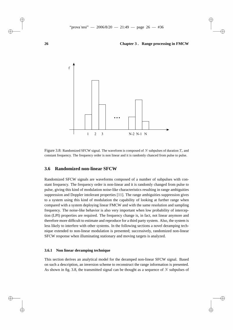
Figure 3.8: Randomized SFCW signal. The waveform is composed of N subpulses of duration Ts andconstant frequency. The frequency order is non linear and it is randomly chanced from pulse to pulse.

3.6 Randomized non-linear SFCW

Randomized SFCW signals are waveforms composed of a number of subpulses with con-stant frequency. The frequency order is non-linear and it is randomly changed from pulse topulse, giving this kind of modulation noise-like characteristics resulting in range ambiguitiessuppression and Doppler intolerant properties [11]. The range ambiguities suppression givesto a system using this kind of modulation the capability of looking at further range whencompared with a system deploying linear FMCW and with the same resolution and samplingfrequency. The noise-like behavior is also very important when low probability of intercep-tion (LPI) properties are required. The frequency change is, in fact, not linear anymore andtherefore more difficult to estimate and reproduce for a third party system. Also, the system isless likely to interfere with other systems. In the following sections a novel deramping tech-nique extended to non-linear modulation is presented; successively, randomized non-linearSFCW response when illuminating stationary and moving targets is analyzed.

3.6.1 Non linear deramping technique

This section derives an analytical model for the deramped non-linear SFCW signal. Basedon such a description, an inversion scheme to reconstruct the range information is presented.As shown in fig. 3.8, the transmitted signal can be thought as a sequence of N subpulses of

“prova˙tesi” — 2006/8/20 — 21:49 — page 27 — #37�

�

�

�

�

�

�

�

3.6 Randomized non-linear SFCW 27

duration Ts and constant frequency fn:

st(t) =N∑

n=1

u

(t − nTs

Ts

)exp

(j(2πfn(t − nTs) + φn)

)(3.23)

where u(t) is the step function defined as 1 for 0 ≤ t < 1 and 0 otherwise, while the phaseterm is equal to:

φn =∫ nTs

Ts

2πfndt (3.24)

in order to guarantee the continuity of the signal phase. The received signal is a delayedversion of the transmitted (any amplitude characteristic is discarded in the present derivation):

sr(t) =N∑

n=1

u

(t − nTs − τ

Ts

)exp

(j(2πfn(t − nTs − τ) + φn)

)(3.25)

In an homodyne receiver the received and transmitted signal are mixed, producing the inter-mediate frequency signal:

sif (t, τ) = st(t)sr(t)∗ =N∑

n=1

N∑k=1

u

(t − nTs

Ts

)u

(t − τ − kTs

Ts

)

exp(j(2π(fn(t − nTs) − fk(t − kTs − τ)) + φn − φk)

)(3.26)

If the sampling frequency is such that one sample is taken for every subpulse, the samplingtime can be written as t = mTs + t0 with 0 ≤ t0 < Ts and 0 ≤ m < N with m ∈ N:

sif (t = mTs + t0, τ) =N∑

n=1

N∑k=1

u

((m − n)Ts + t0

Ts

)u

((m − k)Ts + t0 − τ

Ts

)

exp(j(2π(fn(mTs + t0 − nTs)

−fk(mTs − kTs + t0 − τ)) + φn − φk))

(3.27)

Simplifying:

sif (t = mTs + t0, τ) =N∑

k=1

u

((m − k)Ts + t0 − τ

Ts

)

exp(j (2π (fmt0 − fk(mTs − kTs + t0 − τ)) + φn − φk)

)(3.28)

Expressing τ as lTs + τ0, with l ∈ N and 0 ≤ τ0 < Ts, the time delay is divided in parts,each one of duration equal to Ts. The intermediate frequency signal can be written in the

“prova˙tesi” — 2006/8/20 — 21:49 — page 28 — #38�

�

�

�

�

�

�

�


following way:

sif (t = mTs + t0, τ = lTs + τ0) =N∑

k=1

u

((m − k − l)Ts + t0 − τ0

Ts

)exp

(j(2π

(fmt0 − fk((m − k − l)Ts + t0 − τ0)) + φn − φk))

=

exp(j(2π((fm − fm−l)t0 + fm−lτ0) + φm − φm−l)

)(3.29)

From the previous equation it is clear that all the terms which do not carry any informationabout the target range have to be removed, in order to reconstruct the range information whenthe time delay is larger than the subpulse duration. The phase correction is performed by amultiplication with the following reference function:

exp(− j(2π(fm − fm−l)t0 + φm − φm−l)

)(3.30)

The resulting signal is:

exp(j2πfm−lτ0) (3.31)

Next, a reordering of the samples is performed, such that the corresponding subpulse fre-quency order is linear. This operation allows the use of an FFT to obtain the range profile.However, each of the reference function multiplication and reordering correctly reconstructsonly one part of the time delay profile, depending on the value of l. Each value of l corre-sponds to a constant range interval RTS

. To have the complete range profile, this operationhas to be performed varying the parameter l.

At the cost of increased computation, the described extension of the deramping techniqueto the randomized SFCW allows the use of such a technique not only for linear modulatedsignals, but also for nonlinear ones. The deramping method leads to a lower sampling rateand to a simpler hardware in the radar system: the receiver sampling frequency does not needto be higher than the complete bandwidth (complex sampling) of the transmitted signal, butit has to be only enough to have one sample for every subpulse.

However, some comments on the sampling frequency are required. If a sample is takenduring the transition of one frequency step in the received signal, the resulting phase couldbe not well determined. Having two complex samples per subpulse can solve the problem, atthe cost of an increased processing load.

Nevertheless, the sampling constraints can be drastically reduced especially for high res-olution systems.

3.6.2 Stationary targets

In order to validate the analytical development, a simulation analysis has been performed.A linear and randomized SFCW sequence have been generated with the parameters listedin tab. 3.1, in order to compare the two waveform responses.

“prova˙tesi” — 2006/8/20 — 21:49 — page 29 — #39�

�

�

�

�

�

�

�


Table 3.1: Waveform parameters and target distances for the non linear deramping simulations.

B 1 GHz Ru 150 m

N 1000 RTs150 m

Ts 1 μs target 1 50 m

PRI 1 ms target 2 225 m

PRF 1 kHz target 3 400 m

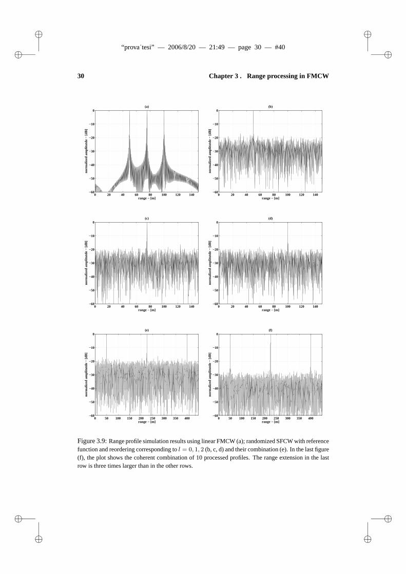
A bandwidth of 1 GHz is transmitted using 1000 subpulses, leading to an unambiguousrange (Ru) of 150 m for linear modulation. The subpulse duration is 1 μs, so the range profileis divided in parts (RTs

) of 150 m extension. It is interesting to note that Ru and RTscoincide

when 1/N = B/Ts, as it is the case in the example used for the simulation.Three stationary targets have been simulated with same power response at ranges such

that their time delay is within one, larger than one and larger than two subpulse duration,respectively. Results are reported in fig. 3.9. It can be seen that only the first target distance iscorrectly measured using a linear SFCW signal (fig. 3.9(a)). In fact, the distance of the othertwo targets is larger than the maximum unambiguous range Ru and therefore folded back.However, using a randomized SFCW, the range ambiguity is suppressed; only the target thatis in the range part correctly reconstructed by the particular phase correction and reorderingis imaged (fig. 3.9(b), 3.9(c), 3.9(d)). Finally, combining the results of the range processingfor different values of l, a complete range profile is obtained (fig. 3.9(e)).

When compared with the linear SFCW output, it is possible to observe the increase ofthe noise floor in the random modulation output, due to the presence of other targets. Infact, their energy is suppressed by spreading it over the range spectrum. Coherent averagingcan reduce this noise floor, as it is illustrated in fig. 3.9(f) where 10 processed sweeps areaveraged, because randomization destroys the sidelobe coherence from sweep to sweep [12],while preserving the target main lobe.

3.6.3 Moving targets

In this section, the response of a moving target illuminated by a randomized stepped fre-quency modulation is briefly mentioned. Opposite to linear modulations, non-linear signalshave the characteristic of being Doppler intolerant, which means that a moving target re-sponse amplitude can be much lower than the corresponding stationary case. The conceptis analytically described by the ambiguity function of the signal; for randomized non-linearstepped frequency it is expressed by:

|χ(τ, fD)|2 = |sinc(Bτ)sinc(fDTp)|2 (3.32)

“prova˙tesi” — 2006/8/20 — 21:49 — page 30 — #40�

�

�

�

�

�

�

�


0 20 40 60 80 100 120 140−60

−50

−40

−30

−20

−10

0

range − [m]

norm

aliz

ed a

mpl

itut

de −

[dB

]

(a)

0 20 40 60 80 100 120 140−60

−50

−40

−30

−20

−10

0

range − [m]

norm

aliz

ed a

mpl

itut

de −

[dB

]

(b)

0 20 40 60 80 100 120 140−60

−50

−40

−30

−20

−10

0

range − [m]

norm

aliz

ed a

mpl

itut

de −

[dB

]

(c)

0 20 40 60 80 100 120 140−60

−50

−40

−30

−20

−10

0

range − [m]

norm

aliz

ed a

mpl

itut

de −

[dB

]

(d)

0 50 100 150 200 250 300 350 400−60

−50

−40

−30

−20

−10

0

range − [m]

norm

aliz

ed a

mpl

itut

de −

[dB

]

(e)

0 50 100 150 200 250 300 350 400−60

−50

−40

−30

−20

−10

0

range − [m]

norm

aliz

ed a

mpl

itut

de −

[dB

]

(f)

Figure 3.9: Range profile simulation results using linear FMCW (a); randomized SFCW with referencefunction and reordering corresponding to l = 0, 1, 2 (b, c, d) and their combination (e). In the last figure(f), the plot shows the coherent combination of 10 processed profiles. The range extension in the lastrow is three times larger than in the other rows.

“prova˙tesi” — 2006/8/20 — 21:49 — page 31 — #41�

�

�

�

�

�

�

�


showing that the Doppler response is a sinc whose width depends on the pulse duration. Incontinuous wave systems, the pulse duration is equal to PRI , therefore the Doppler responsewill have nulls at multiples of PRF .

3.6.4 Influence of hardware non ideality

The previous section has developed an inversion scheme to reconstruct the range profile fromderamped randomized SFCW signals. Basically, when the time delay is larger than the sub-pulse duration, the intermediate frequency signal is undersampled. It can be reconstructedbecause the sequence of the pulse is known. However, the reference function in (3.30) re-quires the value of t0, that is the time instant the sample is taken.

When l is equal to zero (time delay shorter than the subpulse duration) the referencefunction is constant and in this case a simple reordering (and FFT) is enough for the rangereconstruction, but for other values of l the knowledge of the exact value of t0 is important.

By means of simulations, this section analyzes the effect of inaccurate knowledge of thesampling time, due to the jitter of the clock signal, for example. One target is simulated ata distance placed in the second part of the range profile (l = 1) and three range parts arereconstructed (l = 0, 1, 2), as shown in fig. 3.10; in this way the noise floor of the first andthird range part is due to the spreading of the target energy, while the noise floor in the secondrange part is due to the sampling inaccuracy.

Since the spreading induced noise is dominant, the sampling induced noise has to be

0 50 100 150 200 250 300 350 400

−250

−200

−150

−100

−50

0

range − [m]

norm

aliz

ed a

mpl

itut

de −

[dB

]

Figure 3.10: Simulation of only one target placed in the second part of the range profile. In the firstand third part the noise floor is due to the target energy spreading when the deramping is performed forother value of the parameter l in the reference function multiplication and reordering. When jitter ispresent, the noise floor in the second part will rise.

“prova˙tesi” — 2006/8/20 — 21:49 — page 32 — #42�

�

�

�

�

�

�

�


−12 −10 −8 −6 −4 −2 0−20

0

20

40

60

80

100

120

140

160

knj

SSN

R −

[dB

]

1 GHzl00 MHz

Figure 3.11: Spreading induced noise to jitter induced noise ratio plotted versus the knj value and fortwo different values of the transmitted bandwidth.

lower, and for this reason their ratio is used as description parameter. At least one sample persubpulse (complex sampling) has to be taken, therefore the following sampling frequency isused as reference:

fs =N

PRI(3.33)

The jitter is simulated as white noise with maximum amplitude equal to a fraction of thereference sampling frequency and added to the sampling time variable:

t0jitter = t0 + 10knj fswgn(t) (3.34)

where wgn(t) a unitary white gaussian noise function. Simulation results are reported infig. 3.11, where the spreading to sampling induced noise ratio (SSNR) is plotted versus theparameter knj of (3.34). Two curves are obtained, for a transmitted bandwidth of 100 MHzand 1 GHz, respectively, and with 1 MHz as reference sampling frequency (using a PRI of1 ms and N equal to 1000). It is shown how the SSNR increases for lower value of knj andfor lower transmitted bandwidth.

3.7 Summary

The chapter has described the range processing of FMCW data in a complete and detailedmanner. It presented a novel processing solution, developed within the framework of thisthesis, which completely removes the frequency non-linearity effects. It corrects for the non-linearity effects for the whole range profile at once, operates directly on the deramped data

“prova˙tesi” — 2006/8/20 — 21:49 — page 33 — #43�

�

�

�

�

�

�

�

3.7 References 33

and it is very computationally efficient. The removal of the defocusing is range and Dopplerindependent. The integration of the non-linearity correction in FMCW SAR algorithms isdescribed in appendix A. Non linear SFCW modulation has also been treated in the chapter; aderamping technique extended to the case of non linear signals has been introduced. With theextended deramping technique proposed here, reduced sampling frequency as for the linearcase can be used also for randomized SFCW signals, at the cost of increased computation.

References

[1] A. G. Stove, “Linear FM-CW Radar Techniques,” IEE Proc. Part F Radar Signal Pro-cess., vol. 139, no. 5, pp. 343–350, Oct. 1992.

[2] S. O. Piper, “Homodyne FM-CW Radar Resolution Effects with Sinusoidal Nonlinear-ities in the Frequency Sweep,” in Proc. IEEE Int. Radar Conf. ’95, Alexandria, USA,May 1995, pp. 563–567.

[3] D. E. Barrick, “FM-CW Radar Signals and Digital Processing,” in National Oceanicand Atmospheric Administration, Tech. Rep. AD-774-829, July 1973.

[4] S. O. Piper, “FMCW Linearizer Bandwidth Requirements,” in Proc. IEEE Radar Conf.’91, Mar. 1991, pp. 142–146.

[5] M. Vossiek, P. Heide, M. Nalezinski, and V. Magori, “Novel FMCW radar system con-cept with adaptive compensation of phase errors,” in Proc. European Microwave Conf.EuMC’96, Prague, Czech Republic, Sept. 1996, pp. 135–139.

[6] Z. Zhu, W. Yu, X. Zhang, and X. Qiu, “A Correction Method to Distortion in FM-CWImaging System,” in Proc. IEEE Aerospace Electronics Conf. NEACON’96, Dayton,USA, May 1996, pp. 323–326.

[7] M. Edrich, “Design Overview and Flight Test Results of the Miniaturised SAR SensorMISAR,” in Proc. EuRAD’04, Amsterdam, The Netherlands, Oct. 2004, pp. 205–208.

[8] A. Meta, P. Hoogeboom, and L. P. Ligthart, “Range non-linearities correction in FMCWSAR,” in Proc. IEEE Int. Geoscience and Remote Sensing Symp. IGARSS’06, Denver,CO, USA, July 2006.

[9] ——, “Range Frequency Non-linearity Correction for FMCW SAR,” European PatentApplication, no. 06076057.6, May 2006.

[10] W. G. Carrara, R. S. Goodman, and R. M. Majewski, Spotlight Synthetic ApertureRadar. Boston, Artech House Inc., 1995.

[11] J. E. Luminati, T. B. Hale, M. A. Temple, M. J. Havrilla, and M. E. Oxley, “DopplerAliasing Artifacts Filtering in SAR Imagery using randomized Stepped-FrequencyWaveforms,” IEE Electronic Letters, vol. 40, no. 22, pp. 1447–1448, Oct. 2004.

“prova˙tesi” — 2006/8/20 — 21:49 — page 34 — #44�

�

�

�

�

�

�

�

34 REFERENCES

[12] K. Morrison, “Increasing the Effective Bandwidth of an SF-CW SAR using FrequecyAgility,” in Proc. IEEE Int. Radar Conference, Arlington, USA, May 2005, pp. 201–205.

“prova˙tesi” — 2006/8/20 — 21:49 — page 35 — #45�

�

�

�

�

�

�

�

35

Chapter 4

Cross-range imaging with FMCW SAR

The conventional stop-and-go approximation used in pulse radar algorithms can be not valid anymore

in FMCW SAR applications, therefore the motion within the sweep needs to be taken into account. The

chapter presents an analytical development of the FMCW SAR signal model, starting from the deramped

signal and without using the stop-and-go approximation. The novel model is first validated with a

stripmap simulation and then applied to spotlight and single transmitter/multiple receiver Digital Beam

Forming (DBF) synthetic aperture operational modes. In the latter cases, the effect of the motion during

the transmission and reception of the pulse, if not compensated for, can become seriously degrading for

the SAR image quality.

4.1 Introduction

Synthetic Aperture Radar techniques allow a finer resolution in the cross-range direction bysimulating a long antenna array using a single moving sensor. The antenna is usually mountedon an aircraft or satellite, which provide the moving platform. Three categories of motion canbe distinguished during the SAR data collection [1]: motion occurring between successivetransmitted pulses, between transmission and reception of a pulse, and during transmissionand reception. Conventional monostatic SAR algorithms are based on the exploitation of thefirst kind of motion. The second category gives rise to bistatic effects while the motion duringtransmission and reception of the pulse is usually neglected. However, its effect becomesimportant when the pulse duration increases. This is the case when using FMCW radarsensors. They will play an important role in the airborne earth observation field where specialattention is devoted to lightweight, cost-effective imaging sensors of high resolution.

The aim of this chapter is to develop a complete FMCW SAR signal model which takesinto account also the effects of the motion during the sweep. Conventional SAR algorithmshave been developed for pulse radars and are not optimal for the FMCW case. Therefore,when using FMCW sensors, proper algorithms have to be used to achieve the expected re-sults with the maximum resolution. In [2], an algorithm processing FMCW SAR signals ispresented; however, it requires the complete bandwidth of the transmitted signal to be sam-pled and a single long FFT to be performed over the whole collected data for the processing.

“prova˙tesi” — 2006/8/20 — 21:49 — page 36 — #46�

�

�

�

�

�

�

�

36 Chapter 4 . Cross-range imaging with FMCW SAR

In contrast, an algorithm which uses the inherent FMCW deramp-on-receive operation [3] [4][5] is proposed here; in this way, the raw data bandwidth can be drastically reduced, speciallyfor high resolution systems.

The remainder of the chapter is divided into six sections. In section 4.2, a brief heuristicoverview of the FMCW SAR signal is described, indicating when conventional SAR algo-rithms cannot be used, while section 4.3 derives an analytical description of the FMCW SARsignal without any approximation. A stripmap FMCW SAR simulation is reported in sec-tion 4.4. Successively, in section 4.5 and 4.6 the model is applied to spotlight and singletransmitter/multiple receiver operational modes, respectively, where the effect of the motionduring the transmission and reception of the pulse can become seriously degrading for theSAR image quality if not compensated for. The chapter is finalized by section 4.7 whereconclusions are stated.

4.2 Signal processing aspects

For typical pulse SAR systems, the pulse length Tp is sufficiently short for the radar to beassumed stationary during the transmission and the reception of the signal. This is calledthe stop-and-go approximation: while the aircraft is flying it is as if it stops, sends a pulse,receives it and then moves to the next position. Conventional SAR algorithms use this as-sumption and the azimuth compression is achieved by using the geometry of the imagingscenario; the Doppler effect within the sweep is not important because the aircraft is assumedstationary. If the Pulse Repetition Interval is varied, while still properly sampling the in-stantaneous Doppler bandwidth, nothing changes for the SAR processing algorithm [6]. Infig. 4.1 a stripmap SAR geometry is illustrated: θaz is the antenna beamwidth, (x1, y1) arethe coordinates of the scene center, h is the flight altitude and R =

√h2 + y2

1 is the dis-tance between the aircraft trajectory and a parallel line passing through the scene center. If ascatterer is seen by the radar under a look angle γ, the Doppler frequency can be expressedas

fD =2v

cfr sin γ (4.1)

where c is the speed of light, fr is the transmitted frequency. Indicating with γmin and γmax

the minimum and maximum angle under which a scatterer is illuminated, we can introducethe instantaneous BDi and entire Doppler bandwidth BD, respectively defined as:

BDi ≈ 2v

cfc sin θaz (4.2)

BD =2v

cfc(sin γmax − sin γmin) (4.3)

where fc is the center frequency. In order to analyze the effects of the motion within thesweep in FMWC SAR configurations, it is convenient to define the following parameters, theduty cycle η, the oversampling factor μ and the instantaneous to entire Doppler bandwidth

“prova˙tesi” — 2006/8/20 — 21:49 — page 37 — #47�

�

�

�

�

�

�

�

4.2 Signal processing aspects 37

Figure 4.1: SAR system geometry.

ratio ξ, respectively, as:

η = Tp/PRI (4.4)

μ = PRF /BDi (4.5)

ξ = BDi/BD (4.6)

where PRF is the Pulse Repetition Frequency. Finally, we define:

K =BD

δfr(4.7)

as the ratio between the entire Doppler bandwidth and the range frequency resolution δfr,equal to 1/Tp. The parameter K indicates how much the Doppler frequency due to the motionwithin the pulse transmission is comparable to the frequency resolution, and therefore howgood it can be measured. Rearranging the expression in (4.7) in terms of the parametersintroduced above yields:

K =η

μξ(4.8)

Equation (4.8) directly relates K to the radar configuration (η) and SAR operational mode(μ, ξ). For typical pulsed SAR systems K � 1, but when K becomes closer to unity thestop-and-go approximation cannot be considered valid anymore. As we will see in section4.5 and 4.6, in spotlight and multiple tranmitter/receivers SAR modes, ξ and μ, respectively,

“prova˙tesi” — 2006/8/20 — 21:49 — page 38 — #48�

�

�

�

�

�

�

�


can be smaller than unity and, combined with the use of CW sensors (η equal to one), thatmeans the value of K can become even larger than one.

When the stop-and-go approximation is not valid, the frequency of the received signal isbetter described as shifted with respect to the transmitted by an amount equal to the Dopplerfrequency. Figure 4.2 shows qualitatively the signal support band in the two-dimensionalrange spatial frequency Kr and azimuth spatial frequency Kx domain for a wideband FMCWSAR. The support band will differ from the usual representation because it is squinted; how-ever, the most important aspect is that the ”frequency of the signal” in the two-dimensionalfrequency domain will also be shifted by the appropriate Doppler component.

Figure 4.2: Pulse SAR and FMCW SAR support band in the two-dimensional spatial frequency do-main. The squinting is exaggerated for purposes of clarity.

“prova˙tesi” — 2006/8/20 — 21:49 — page 39 — #49�

�

�

�

�

�

�

�

4.3 Analytical development 39

4.3 Analytical development

This section derives an analytical development for the description of the FMCW SAR signalin the two-dimensional frequency domain. The radar continuously transmits linear FM chirpshaving duration Tp equal to the PRI , chirp rate α = B/PRI , where B is the transmittedbandwidth and center frequency fc, see fig. 4.3. The transmitted frequency is expressed as:

fr = fc + αt (4.9)

where −PRI/2 ≤ t < PRI/2. In dechirp-on-receive systems, the received and transmittedsignal are mixed in order to reduce the required system sampling rate. The intermediatefrequency signal SIF output of the mixer is:

SIF = exp(

j2π

(fcτ + ατt − 1

2ατ2

))(4.10)

The last term is an unwanted phase term known as Residual Video Phase (RVP) [1]; it isusually negligible, or otherwise can be corrected. In the rest of the analysis, it is assumedremoved. A more general model including frequency non-linearities and RVP is derived inappendix A, where also a novel and efficient processing algorithm for FMCW SAR data isintroduced. The time delay τ due to a point target located in the center of the scene is:

τ =2r (R, x1, t

′)c

=2√

R2 + (vt′ − x1)2

c

=2√

R2 + (xn + vt − x1)2

c(4.11)

where t′ = Tn + t is the continuous time variable and Tn = nPRI , with n integer, is whatis usually referred to as slow time variable; xn = vTn is the position of the aircraft along its

Figure 4.3: Chirp pulse in the frequency-time domain. The received signal (dotted) is a delayedversion of the transmitted one (solid). If a Doppler effect is present, the received signal will be shiftedin frequency of an amount proportional to the instantaneous frequency (dashed).

“prova˙tesi” — 2006/8/20 — 21:49 — page 40 — #50�

�

�

�

�

�

�

�


ideal straight line path, at regular time intervals.

The intermediate frequency signal (without the RVP term) is written as:

SIF (Kr, xn) = exp (j2π (fcτ + ατt)) = exp (jKrr)

= exp(jKr

√R2 + (xn + vt − x1)2

)(4.12)

where the spatial range frequency is equal to:

Kr =4π

cfr =

4π

cα

(fc

α+ t

)= Krc + ΔKr (4.13)

where Krc is the central range spatial frequency and ΔKr is its variation around Krc. Inorder to obtain an expression for the FMCW SAR signal in the two-dimensional frequencydomain, a Fourier transform with respect to the variable xn is performed on (4.12) (from nowon we suppress the subscript n in the variable xn, and we refer to it simply as x):

Fx (SIF ) =∫

exp(jKr

√R2 + (x + vt − x1)2 − jKxx

)dx (4.14)

Using the substitution x′ = x + vt, the integral in (4.14) can be rewritten as:∫exp

(jKr

√R2 + (x′ − x1)2

)exp (−jKx(x′ − vt)) dx′ (4.15)

Bringing the exponential term exp(jKxvt) out of the integral and solving it by means of theprinciple of the stationary phase yields:

SIF (Kr,Kx) = exp (jKxvt) exp(jR

√K2

r − K2x − jKxx1

)(4.16)

Equation (4.16) describes the FMCW SAR signal in the two-dimensional spatial frequencydomain. It differs from the conventional description in the presence of the first exponentialterm. This is a space-invariant term that takes into account the motion within the sweep,leading to a more general solution.

The stop-and-go approximation assumes the radar stationary while transmitting and re-ceiving the pulse, so v is equal to zero; in (4.16) the first exponential term would disappearreverting to the conventional pulse SAR equation [1][2]. However, since the derived expres-sion is a more general description of the SAR signal, it has to hold also when the true velocityvalue is inserted. In fact, the variation of t is very small compared with the product Kxv inpulse radar cases and therefore the phase of the first exponential is practically constant.

4.4 Stripmap FMCW SAR simulation

For a first validation of the derivation, a stripmap FMCW SAR simulation of one targethas been carried out with the following parameters: carrier frequency fc = 10 GHz, trans-mitted bandwidth 500 MHz, PRI = 1 ms, antenna beamwidth 10o, squint angle 20o, target

“prova˙tesi” — 2006/8/20 — 21:49 — page 41 — #51�

�

�

�

�

�

�

�

4.5 Spotlight FMCW SAR 41

range distance R = 403 m and aircraft velocity v = 50 m/s, leading to a value of K equalto 0.46. After the raw data are generated according to (4.10), a range deskew operation isperformed to remove the RVP and then an FFT in the azimuth direction makes the signal inthe two-dimensional frequency domain available. In order to compare the conventional andthe described SAR model, the signal in the two-dimensional frequency domain is matchedfiltered with the conventional and proposed reference function for the range of the simulatedtarget. Figure 4.4(a) shows the real part after matched filtering with a reference function thatdoes not take into account the motion within the sweep (stop-and-go approximation) whilefig. 4.4(b) has been produced by filtering the signal with our proposed model expressed in(4.16). Only in the last picture the phase is practically constant, indicating that the referencefunction really matches the scatterer signal.

Doppler frequency − [Hz]

Ran

ge f

requ

ency

− [

GH

z]

(a)

700 800 900 1000 1100 1200 1300 1400 1500 16009.75

9.8

9.85

9.9

9.95

10

10.05

10.1

10.15

10.2


Ran

ge f

requ

ency

− [

GH

z](b)

700 800 900 1000 1100 1200 1300 1400 1500 16009.75

9.8

9.85

9.9

9.95

10

10.05

10.1

10.15

10.2

Figure 4.4: Stripmap simulation results: real part of the two-dimensional domain for a target in thescene center after conventional (a) and proposed (b) matched filtering.

4.5 Spotlight FMCW SAR

In spotlight mode SAR, the antenna beamwidth is not constrained to a fixed direction, but itcan be steered in order to illuminate a certain area for a longer period. In this way, the angleunder which a target can be observed is not limited by the antenna beamwidth and thereforea larger Doppler bandwidth is available, leading to a better achievable azimuth resolution.For a larger Doppler bandwidth, a larger PRF should be used in order to correctly sample theSAR signal. However, it is important to note that at every instant a sample is taken, the actualDoppler bandwidth observed by the SAR system is limited by the antenna beamwidth. ThePRF has to be high enough to sample this instantaneous bandwidth, therefore the bandwidthto take into account for the Nyquist theorem formulation is the instantaneous bandwidth andnot the complete Doppler bandwidth. In order to correctly reconstruct the Doppler band-width, the azimuth data are processed in a similar way to the ramping of the deramped rangesignal [7]. The technique is briefly reviewed. The SAR raw data are modulated in cross-range

“prova˙tesi” — 2006/8/20 — 21:49 — page 42 — #52�

�

�

�

�

�

�

�


direction by an hyperbolic function that depends on the range frequency Kr and target rangehistory:

s(Kr, x) = exp(jKr

√R2 + (x + vt − x1)2) (4.17)

In order to compress the signal bandwidth, the raw data are multiplied with the referencefunction:

sref (Kr, x) = exp(−jKr

√R2

0 + x2) (4.18)

where R0 is a reference range, i.e. the range at the center of the scene. This reference functionis sampled at the same frequency as the raw data, that is at PRF . The compressed signal

scomp(Kr, x) = s · sref (4.19)

has a reduced bandwidth and it can be used to reconstruct the original bandwidth. In fact, itis not aliased anymore and can be upsampled (using zero padding and FFT) at a frequencymPRF , with m large enough such that mPRF > BD. Finally, multiplying the upsampledcompressed signal with the reference function (also sampled now at mPRF ), the originalsignal is reconstructed without aliasing.

In such a scenario, the image degradation can be quite high if the effects of the motionwithin the sweep are not corrected for because the Doppler bandwidth can be larger than thePRF (ξ < 1, μ > 1), differently from the stripmap case. In fact, every time the Doppler band-width extends of a PRF value, the response in range direction migrates of one resolution cell.This is demonstrated in fig. 4.5 by means of simulated data, where the following parametersare used: carrier frequency fc = 10 GHz, transmitted bandwidth 500 MHz, PRI = 4 ms,illumination angle 20o, squint angle 10o, target range distance R = 120 m and aircraft ve-locity v = 40 m/s. The choice of these parameters results in a value of K equal to 3.64. Theparameter K does not depend on the target range value. Therefore, the low range value waschosen for the simulation only for computational reasons. Similar to the stripmap example,the raw data are first generated according to (4.10), processed in order to reconstruct the una-liased signal with the technique previously described, Fourier transformed with respect to thecross-range direction and finally matched filtered with both the conventional SAR referencesignal and the proposed one, expressed by (4.16). The results are shown in fig. 4.5, where theimprovements due to the proposed correction are clearly visible.

4.6 Digital beam forming FMCW SAR

Spotlight mode gives the advantage of higher cross range resolution compared to stripmapmode, at the expense of a reduced imaged area. In both the operational modes, the imageswath is limited by the PRF in conventional radars; its value is determined by the maximumallowable distance travelled by the radar platform between successive transmitted pulses andby the fact that the PRF has to be high enough to sample the instantaneous clutter Dopplerbandwidth.

“prova˙tesi” — 2006/8/20 — 21:49 — page 43 — #53�

�

�

�

�

�

�

�

4.6 Digital beam forming FMCW SAR 43


Ran

ge f

requ

ency

− [

GH

z]

(a)

0 100 200 300 400 500 600 700 800 9009.75

9.8

9.85

9.9

9.95

10

10.05

10.1

10.15

10.2


Ran

ge f

requ

ency

− [

GH

z]

(b)

0 100 200 300 400 500 600 700 800 9009.75

9.8

9.85

9.9

9.95

10

10.05

10.1

10.15

10.2

10.25

1290 1300 1310 1320 1330 1340

195

200

205

210

215

220

225

230

Ran

ge b

in

Cross−range bin

(c)

1290 1300 1310 1320 1330 1340185

190

195

200

205

210

215

220

225R

ange

bin

Cross−range bin

(d)

160 180 200 220 240 260−60

−50

−40

−30

−20

−10

0

Range bins

Nor

mal

ized

pow

er −

[dB

]

(e)

conventionalFMCW

1200 1250 1300 1350 1400−60

−50

−40

−30

−20

−10

0(f)

Cross−range bins

Nor

mal

ized

pow

er −

[dB

]

conventionalFMCW

Figure 4.5: Spotlight simulation results for K equal to 3.64; real part of the two-dimensional domainfor a target in the scene center after conventional (a) and proposed (b) matched filtering; contour plotsof the resulting point response (c, d) and range and cross-range profile comparison (e, f).

“prova˙tesi” — 2006/8/20 — 21:49 — page 44 — #54�

�

�

�

�

�

�

�


These limitations are overcome by using multiple channels in Digital Beam Forming SARconfiguration. In general, a DBF SAR consists of an array of transmitters and receivers. IfN is the number of receivers, at every instant, N data streams are recorded and from everychannel a SAR image can be produced. Proper processing of the N channels allows a low-ering of the PRF [8]. This means that a larger swath can be imaged, still correctly samplingthe clutter Doppler bandwidth. In fact, the signal from a single channel will be undersampledin the cross-track direction; however the complete Doppler spectrum can be reconstructed bycombining the information of the whole receive subarrays. Every transmitter/receiver bistaticconfiguration can be thought as a monostatic sensor placed in between them [9], and thereforeN samples are available at the same time in the spatial domain, allowing a PRF reductionof the same factor N . As shown in fig. 4.6 for a single transmitter/ multiple receivers case,the spatial sampling is reduced from di, the space one single antenna has moved during onesweep, to dN , the distance of two adjacent subarray phase center, after DBF processing.

In the present discussion, we will assume the aircraft velocity such that the resulting sam-ples are equally spaced in the azimuth direction. The removal of this limitation is treated inliterature [10], and is not relevant for the topic discussed in this section. The focus here is thefact that the PRF of the single channel is lower than the instantaneous clutter Doppler band-width (μ < 1). As described in the previous sections, this results in performance degradationswhen conventional SAR processing algorithms are used, neglecting therefore the effects ofthe motion during the sweep.

A simulation with the following parameters has been performed: single transmitter, 5receivers, carrier frequency fc = 40 GHz, transmitted bandwidth 500 MHz, PRI = 1 ms,

Figure 4.6: Digital beam forming principle.

“prova˙tesi” — 2006/8/20 — 21:49 — page 45 — #55�

�

�

�

�

�

�

�

4.6 Digital beam forming FMCW SAR 45


Ran

ge f

requ

ency

− [

GH

z]

(a)

−2500 −2000 −1500 −1000 −500 0 500 1000 1500 200039.75

39.8

39.85

39.9

39.95

40

40.05

40.1

40.15

40.2


Ran

ge f

requ

ency

− [

GH

z]

(b)

−2500 −2000 −1500 −1000 −500 0 500 1000 1500 200039.75

39.8

39.85

39.9

39.95

40

40.05

40.1

40.15

40.2

2 4 6 8 10 12 14 16 18 20

2

4

6

8

10

12

14

16

18

20

Cross−range bins

Ran

ge b

ins

(c)

2 4 6 8 10 12 14 16 18 20

2

4

6

8

10

12

14

16

18

20

Cross−range bins

Ran

ge b

ins

(d)

2 4 6 8 10 12 14 16 18 20−40

−35

−30

−25

−20

−15

−10

−5

0

Range bins

Nor

mal

ized

pow

er −

[dB

]

(e)

conventionalFMCW

2 4 6 8 10 12 14 16 18 20−40

−35

−30

−25

−20

−15

−10

−5

0

Cross−range bins

Nor

mal

ized

pow

er −

[dB

]

(f)

conventionalFMCW

Figure 4.7: Digital Beam Forming simulation results for K equal to 2.8; real part of the two-dimensional domain for a target in the scene center after conventional (a) and proposed (b) matchedfiltering; contour plots of the resulting point response (c, d) and range and cross-range profile compari-son (e, f).

“prova˙tesi” — 2006/8/20 — 21:49 — page 46 — #56�

�

�

�

�

�

�

�

46 REFERENCES

illumination angle 6o, range distance R = 300 m and aircraft velocity v = 100 m/s. Theresulting K is 2.8. Simulation outcomes are shown in fig. 4.7. The response behavior issimilar to the spotlight example of the previous section, but less accentuated due to a lowervalue of K.

4.7 Summary

In this chapter, the FMCW SAR signal description in the two-dimensional frequency domainhas been derived without any approximation. From this model an algorithm that corrects forthe motion within the sweep has been proposed. If conventional algorithms are used, themotion within the sweep is not taken into account and this results in resolution degradation.In FMCW SAR systems, the proposed correction leads to a better image quality. The effectsof the motion during transmission and reception of the pulse become noticeable when themaximum Doppler frequency is comparable to or larger than the range frequency resolution,equal to the PRF in CW systems. Therefore, in operational mode where the PRF can belower than the entire Doppler bandwidth, as can be the case for spotlight and multiple receiversystems, the degradation induced by the motion within the sweep can seriously decrease thequality of the image. Applying the model developed in the chapter, deramped linear FMCWSAR data can be correctly processed and theoretical results are obtained. The integration ofthe non-linearity correction in FMCW SAR algorithms is described in appendix A, leadingto a more general and efficient processing algorithm for FMCW SAR data.

References

[1] W. G. Carrara, R. S. Goodman, and R. M. Majewski, Spotlight Synthetic ApertureRadar. Boston, Artech House Inc., 1995.

[2] M. Soumekh, Fourier Array Imaging. Prentice Hall Inc., 1994.

[3] J. J. M. de Wit, A. Meta, and P. Hoogeboom, “Modified range-Doppler processing forfm-cw synthetic aperture radar,” IEEE Geosci. Remote Sensing Letters, vol. 3, no. 1, pp.83–87, Jan. 2006.

[4] A. Meta and P. Hoogeboom, “Signal Processing Algorithms for FMCW Moving TargetIndicator Synthetic Aperture Radar,” in Proc. IEEE Int. Geoscience and Remote SensingSymp. IGARSS’05, Seoul, Korea, July 2005, pp. 316–319.

[5] A. Meta, P. Hoogebbom, and L. P. Ligthart, “Correction of the effects induced by thecontinuous motion in FMCW SAR,” in Proc. IEEE Radar Conf. ’06, Verona, NY, USA,Apr. 2006, pp. 358–365.

[6] D. C. Munson and R. L. Visentin, “A Signal Processing View of Strip-Mapping Syn-thetic Aperture Radar,” IEEE Trans. on Acoustic Speech and Signal Processing, vol. 37,no. 12, pp. 2131–2147, Dec. 1989.

“prova˙tesi” — 2006/8/20 — 21:49 — page 47 — #57�

�

�

�

�

�

�

�

REFERENCES 47

[7] M. Soumekh, D. A. Nobles, M. C. Wicks, and G. R. J. Genello, “Signal Process-ing of Wide Bandwidth and Wide Beamwidth P-3 SAR Data,” IEEE Transactions onAerospace and Electronic Systems, vol. 37, no. 4, pp. 1122–1141, Oct. 2001.

[8] P. Barton, “Digital beam forming for radar,” IEE Proceedings, vol. 127, no. 4, Aug.1980.

[9] M. Soumekh, “Bistatic synthetic aperture radar inversion with application in dynamicobject imaging,” IEEE Transactions on Signal Processing, vol. 39, no. 9, pp. 2044–2055, Sept. 1991.

[10] M. Youwn, Digital Beam-Forming for High Resolution Wide Swath Real and SyntheticAperture Radar. Karlsruhe University, Ph. D. thesis, 2004.

“prova˙tesi” — 2006/8/20 — 21:49 — page 48 — #58�

�

�

�

�

�

�

�

48 REFERENCES

“prova˙tesi” — 2006/8/20 — 21:49 — page 49 — #59�

�

�

�

�

�

�

�

49

Chapter 5

Moving Targets and FMCW SAR

The chapter exploits the peculiar characteristics of the complex FMCW SAR image for Moving Target

Indication (MTI) purposes. Two SAR MTI methods are proposed. The first is based on the frequency

slope diversity in the transmitted modulation by using linear triangular FMCW SAR. The second makes

use of the Doppler filtering properties of randomized SFCW modulations.

5.1 Introduction

There is a need in several applications for the detection of ground moving targets and theestimation of their velocity. The motion of ground-based moving target such as car, truckor military vehicle, causes the radar signature of the moving target to shift outside of thenormal ground return of a imaging radar. The problem of detecting slow moving vehiclesin a land clutter environment is compounded by the fact that a significant portion of theuseful signal bandwidth from the antenna’s main lobe and sidelobe is often occupied by theground return. When a single channel radar is used, the minimum detectable velocity of thetarget must be high enough to be clear of the main lobe and sidelobe clutter for robust targetdetection. The moving target Doppler shift from the clutter region is caused by the radialvelocity component. Since the Doppler domain is sampled at the pulse repetition frequency,the available region extension is limited; moving targets with radial velocity high enough canhave their Doppler spectrum folded back in the clutter region, and therefore they cannot bediscriminated from stationary returns by frequency detection. Usually, in pulse SAR radars,the PRF can be chosen high enough for the unambiguous velocity to be less unlikely tooccur; however, a large pulse duration, and therefore a low PRF , is desirable in FMCW SARbecause this relaxes the sampling requirements and the circuitry complexity for a given rangeresolution and maximum range.

The chapter proposes two novel methods to discriminate moving targets which have theirDoppler spectrum folded back in the clutter region. The first is based on the frequency slopediversity in the transmitted modulation by using linear triangular FMCW SAR while thesecond makes use of the Doppler filtering properties of randomized SFCW modulations.

“prova˙tesi” — 2006/8/20 — 21:49 — page 50 — #60�

�

�

�

�

�

�

�

50 Chapter 5 . Moving Targets and FMCW SAR

5.2 Moving target Doppler spectrum

This section reviews the effects induced by the radial velocity component of a moving targeton its Doppler spectrum. A stripmap mode case is analyzed and the scenario is illustratedin fig 5.1. Clutter spectrum response is approximately a chirp-like spectrum, whose band-

Figure 5.1: Moving target with radial velocity component in a stripmap scenario.

width is proportional to the antenna beamwidth, centered around the Doppler centroid, equalto zero for broadside SAR mode. The movement of a target induces a Doppler frequencyproportional to the radial velocity, causing a shift of the target response. Figure 5.2(a) quali-tatively represents the Doppler spectrum of a scenario where clutter, a slow and a fast movingtarget are present. The bandwidth of the slow moving target is almost completely covered bythe clutter spectrum, while the fast moving target spectrum is in a clutter free region.

One simple MTI method makes use of the Doppler shift induced by the radial velocityof the moving target [1]. When the Doppler shift is high enough to have the moving targetspectrum outside the clutter region, the latter can be filtered out and only signatures of movingobjects remain in the SAR data. However, this technique has two limitations:

1. slow moving targets can be suppressed as well, since their spectrum can still be in theclutter region. This limitation is due to the fact that only one antenna is used. Withmore antennas, a spatial dimension is added to the range and Doppler information ofusual SAR images, allowing the discrimination between angle of arrival and Dopplerfrequency, therefore enhancing the separation between clutter and slow moving targets[2][3];

2. moving targets with Doppler shift multiple of PRF will have their spectrum foldedback into the clutter region. In fact, SAR data are sampled in the along track direction

“prova˙tesi” — 2006/8/20 — 21:49 — page 51 — #61�

�

�

�

�

�

�

�

5.3 MTI with linear triangular FMCW SAR 51

with a sampling frequency equal to PRF . That means, the accessible Doppler infor-mation is between ±PRF /2 and all the Doppler spectrum is mapped in this region,see fig. 5.2(b).

Figure 5.2: Doppler spectrum of clutter, a slow and a fast moving target.

Using a linear FMCW modulation, the Doppler region available for moving targets canbe increased by having a larger PRF . However, transmitting the same bandwidth and usingthe same sampling frequency, also the frequency rate of the chirp is increased of the samefactor therefore limiting the maximum range.

5.3 MTI with linear triangular FMCW SAR

This section provides a description of the effects of a moving target as they appear in anFMCW SAR image [4]; the results can be used to assist MTI capabilities. In conventionalSAR systems, it is known from literature [1], that a moving target, when compared to astationary target, is imaged smeared in range and shifted in azimuth because of its radialvelocity and defocused as a consequence of its cross-range velocity and radial acceleration.The main aspect of this section is to emphasize the effect of the target radial velocity vr on theFMCW SAR image. A broadside stripmap narrow-bandwidth and narrow-beamwidth case is

“prova˙tesi” — 2006/8/20 — 21:49 — page 52 — #62�

�

�

�

�

�

�

�


analyzed. The distance between the radar and the moving target is for a broadside mode:

r (R, x, t) =√

(R − vrt′)2 + (vt′ − x1)2

≈ R − ax − vrt +x2

2R= rst − ax − vrt (5.1)

where a = vr/v, rst = R + x2/2R is the equivalent range distance if the target is stationaryand the remaining variables are as defined in chapter 4. By using (5.1) in the equation forSIF , expressed in (4.12), yields:

SIF = exp (jKrr) ≈ exp (jKr (rst − ax − vrt))

≈ exp(

jKrc (rst − ax) + jΔKr

(rst − ax − fcvr

α

))(5.2)

After range compression, Fourier transforming the data with respect to the variable ΔKr, thefollowing is obtained:

s (r′, x) = sinc(

1ρr

(r′ −

(R − ax +

x2

2R− fcvr

α

)))

exp(

jKrc

(R − ax +

x2

2R

))(5.3)

where ρr = c/2B is the image range resolution. In the exponential in (5.3), the linear term inx causes the Doppler spectrum of the moving target to be shifted with respect to the stationarycase by an amount of fD = 2vr/λc, where λc is the wavelength at the carrier frequency. Thisleads to the well known displacement in azimuth Δx of the moving target when displayed ina SAR image:

Δx = Rvr

v=

Rλc

2vfD =

L

v

d

2fD = ρaz

fD

δfD(5.4)

where L is the SAR observation length for a distance R, d is the antenna length, ρaz is theazimuth resolution and δfD is the frequency resolution for the observation length L in theDoppler domain. If Δx is larger than L, the response in the image is shifted by [1]:

Δximag =((

Δx +L

2

)modulo L

)− L

2(5.5)

and this is due to the ambiguity of PRF in the measurement of the Doppler frequency. Fromthe sinc function in (5.3) it is possible to see that the term ax causes the range smearing ofthe moving target image, and that the term fcvr/α shifts the response in the range directionof:

ΔR =fcvr

α=

c

2B

fc

c2vrPRI = ρr

fD

PRF= ρr

fD

δfr(5.6)

where δfr is the range frequency resolution equal to the PRF (twice the PRF for symmetrictriangular modulations). The range shift is a typical characteristic of FMCW radars [5] and it

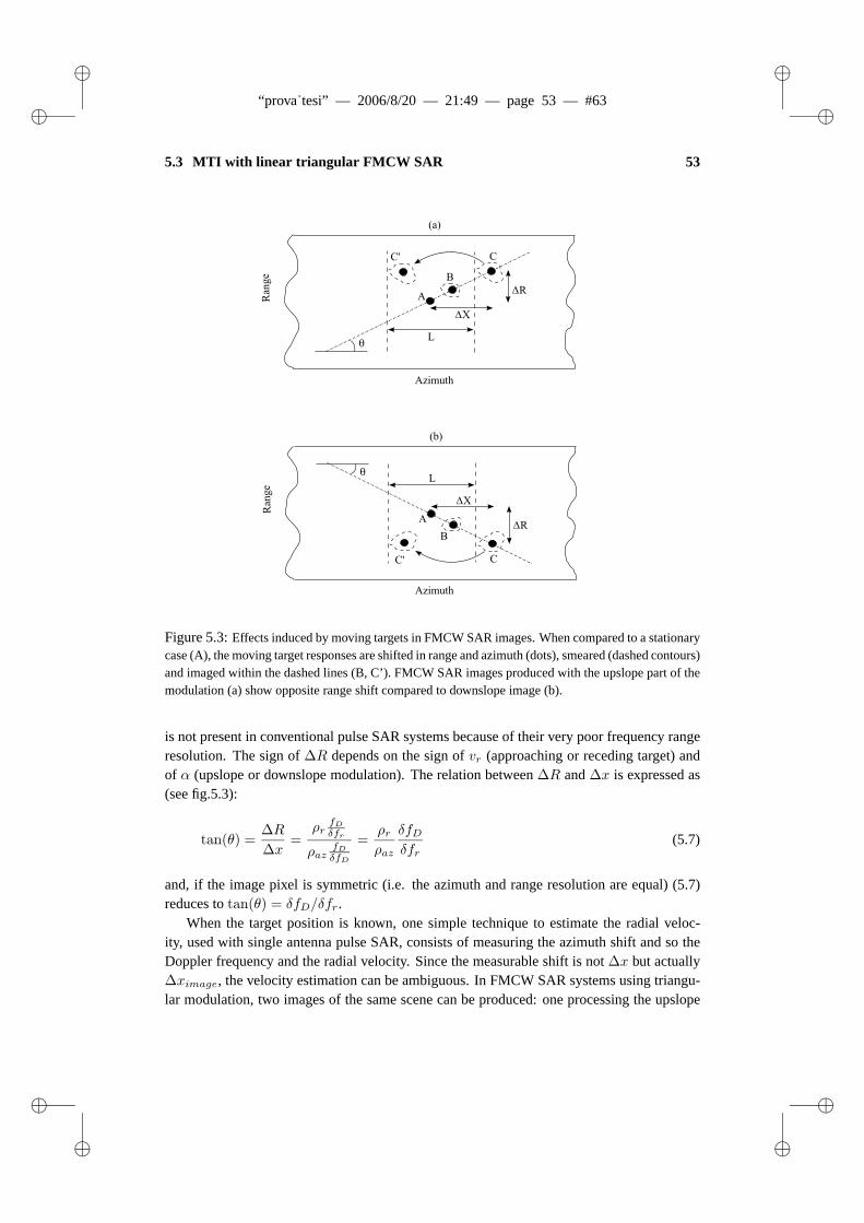
“prova˙tesi” — 2006/8/20 — 21:49 — page 53 — #63�

�

�

�

�

�

�

�

5.3 MTI with linear triangular FMCW SAR 53

Figure 5.3: Effects induced by moving targets in FMCW SAR images. When compared to a stationarycase (A), the moving target responses are shifted in range and azimuth (dots), smeared (dashed contours)and imaged within the dashed lines (B, C’). FMCW SAR images produced with the upslope part of themodulation (a) show opposite range shift compared to downslope image (b).

is not present in conventional pulse SAR systems because of their very poor frequency rangeresolution. The sign of ΔR depends on the sign of vr (approaching or receding target) andof α (upslope or downslope modulation). The relation between ΔR and Δx is expressed as(see fig.5.3):

tan(θ) =ΔR

Δx=

ρrfD

δfr

ρazfD

δfD

=ρr

ρaz

δfD

δfr(5.7)

and, if the image pixel is symmetric (i.e. the azimuth and range resolution are equal) (5.7)reduces to tan(θ) = δfD/δfr.

When the target position is known, one simple technique to estimate the radial veloc-ity, used with single antenna pulse SAR, consists of measuring the azimuth shift and so theDoppler frequency and the radial velocity. Since the measurable shift is not Δx but actuallyΔximage, the velocity estimation can be ambiguous. In FMCW SAR systems using triangu-lar modulation, two images of the same scene can be produced: one processing the upslope

“prova˙tesi” — 2006/8/20 — 21:49 — page 54 — #64�

�

�

�

�

�

�

�


part of the received signal and another one using the downslope. After correction of the mo-tion within the sweep described in chapter 4, stationary targets are imaged in the same wayin the two pictures, while the moving target has the same shift in the azimuth direction butopposite shift in the range direction. Once ΔR is estimated, Δx is derived from (5.7) andso the radial velocity estimated without ambiguity. This technique, like the previous one de-scribed for the pulse SAR system, works properly if the range shift can be observed, i.e. if themoving target is visible in both the images. In order to detect changes induced by the motionof the targets in the two images, standard interferometric deformation techniques can be used[6]. The processing block diagram is shown in fig. 5.4. An example of the application of themethod on real data is reported in section 7.8.

Figure 5.4: MTI with triangular FMCW modulation. The original raw data (a) is divided in twosequences containing the upslope (b) and downslope (c) part, respectively. From each of them, oneFMCW SAR image is produced and successively the two are processed using interferometric deforma-tion techniques in order to detect changes induced by moving targets.

“prova˙tesi” — 2006/8/20 — 21:49 — page 55 — #65�

�

�

�

�

�

�

�

5.4 MTI with randomized non-linear SFCW SAR 55

5.4 MTI with randomized non-linear SFCW SAR

Randomized non-linear SFCW signals have been introduced in section 3.6. This class ofmodulation can be described as noise like signals, which have the property of suppressingrange ambiguities and being Doppler intolerant. In [7], a randomized SFCW modulation hasbeen used in SAR imaging to mitigate the effects of Doppler aliasing due to the undersam-pling of the Doppler bandwidth, especially if the PRF is limited and the antenna beamwidthlarge. This technique is based on the fact that the stepped frequency order inside the pulseis randomly changed from pulse to pulse. After collection of an adequate number of pulses,signal compression leads to a composite ambiguity function equal to:

|χ(τ, fD)|2 = |sinc(Bτ)sinc(fDTp)|2 (5.8)

where B is the transmitted bandwidth, τ is the range time delay, fD the Doppler frequencyand Tp is the time duration of the complete stepped frequency waveform. In most of theusual applications, SAR Doppler aliasing artifacts occur at multiples of the PRF ; choosingTp equal to Pulse Repetition Interval (PRI = 1/PRF ), that means Continuous Wave (CW)operation mode, the artifacts will be removed by the range compression operation.

In the present section, the technique is extended to the case of moving targets [8]. It isknown from SAR literature [9] that imaging a moving target is equivalent to squint modeSAR processing of a stationary target. The equivalent squint angle depends on the targetvelocity; therefore, there are certain velocities that induce a squint angle such that the movingtarget Doppler bandwidth falls over (due to the undersampling) in the clutter region. It is notpossible to discriminate these moving targets using solely the Doppler information. However,with the randomized technique it is possible to produce an ambiguity function that minimizethe clutter return and enhance MTI capabilities.

The aim of this section is to describe how to use non-linear SFCW signals to enhancethe indication of a certain category of moving targets in SAR images using systems with asingle antenna. Using randomized SFCW signals, the composite ambiguity function is wellapproximated by (5.8), indicating that the nulls of the sinc function in the Doppler directionare placed at multiples of 1/Tp. In CW signals, the pulse duration is equal to the PRI andtherefore the nulls are at multiples of the PRF . In this way, range compressing the raw SARsignal (with matched filtering or with deramping technique described in section 3.6) with theproper Doppler frequency, it is possible to suppress the clutter return and to have only theDoppler region of interest. This is obtained multiplying the raw SAR data with the followingfunction:

exp(j2πfDt) (5.9)

where fD is the Doppler of interest and −PRI /2 < t < PRI /2. Successively, range andazimuth processing is performed.

In order to validate the concept, simulations have been performed. Ten stationary andmoving targets have been simulated with the parameters listed in tab. 5.1 and represented in

“prova˙tesi” — 2006/8/20 — 21:49 — page 56 — #66�

�

�

�

�

�

�

�


Table 5.1: Target scenario for the moving target simulations

Scatterer Range Azimuth Doppler

Number (m) (m) (PRF )

1 350 -3 0

2 340 3 0

3 300 -3 0

4 290 3 0

5 250 -3 0

6 240 3 0

7 270 -1 -0.5

8 310 -1 -1

9 305 2 0.5

10 260 2 1

Figure 5.5: Moving and stationary target scenario for the randomized SFCW SAR MTI simulation.

“prova˙tesi” — 2006/8/20 — 21:49 — page 57 — #67�

�

�

�

�

�

�

�


fig. 5.5, while the radar parameters are the same as reported in tab. 3.1, except the transmit-ted bandwidth, reduced to 100 MHz in this simulation. The radar platform velocity and theantenna beamwidth values have been set to 50 m/s and 8o, respectively. A broadside case hasbeen analyzed, and using a 10 GHz carrier frequency results in a clutter Doppler extensionof 500 Hz centered around zero Doppler. The moving targets travel along the radial directionwith velocities such that their spectrum is shifted by the amount reported in the last columnof tab. 5.1. Both linear and randomized SFCW signals have been generated; the azimuthcompression processes a bandwidth of 250 Hz centered around zero Doppler. Resulting SARimages are shown in fig. 5.6. In fig. 5.6(a), the image obtained using linear SFCW modu-lation is reproduced; it can be noticed that stationary targets are correctly imaged, as wellas target 8 and 10 (only some range blurring is observable, due to the range migration). Infact, the Doppler spectrum of target 8 and 10 is folded back in the clutter region and thereforetheir phase history matches the SAR reference compression function. This also means thatfiltering out the clutter region will suppress these two moving targets. Obviously, target 7and 9 are not imaged because their spectrum is outside the processed bandwidth; they can bedetected processing the remaining part of the Doppler spectrum.

Using randomized SFCW modulation, the Doppler filtering is performed directly dur-ing the range compression, reducing in this way aliasing problems. Results are reported infig. 5.6(b), 5.6(c) and 5.6(d): the three images have been produced centering the Dopplerregion of interest to zero, -PRF and +PRF , respectively. It is evident how the three differ-ent Doppler regions can be suppressed separately, enhancing in this way the moving targetindication capability.

A close up view of the normalized amplitude cross-range profile of the correspondingSAR images of fig. 5.6 is shown in fig. 5.7. The two curves are the responses of thestationary target 5 (solid line) and of the moving target 10 (dot-dashed line). By compar-ing fig. 5.7(b) with fig. 5.7(c) and fig. 5.7(d), clutter suppression can be quantified to beapproximately 25 dB.

“prova˙tesi” — 2006/8/20 — 21:49 — page 58 — #68�

�

�

�

�

�

�

�


Cross range − [m]

Ran

ge −

[m

]

(a)

−10 −5 0 5 10

200

220

240

260

280

300

320

340

360

380

400

Cross range − [m]

Ran

ge −

[m

]

(b)

−10 −5 0 5 10

200

220

240

260

280

300

320

340

360

380

400

Cross range − [m]

Ran

ge −

[m

]

(c)

−10 −5 0 5 10

200

220

240

260

280

300

320

340

360

380

400

Cross range − [m]

Ran

ge −

[m

]

(d)

−10 −5 0 5 10

200

220

240

260

280

300

320

340

360

380

400

Figure 5.6: Moving target simulations. SAR images produced when transmitting linear SFCW (a)and when using randomized SFCW with range compression relative to zero, minus one and plus onetime the PRF , (b), (c), (d) respectively. In the latter cases, it is possible to discriminate moving andstationary targets.

“prova˙tesi” — 2006/8/20 — 21:49 — page 59 — #69�

�

�

�

�

�

�

�


−2 0 2 4 6 8−50

−45

−40

−35

−30

−25

−20

−15

−10

−5

0

Cross range − [m]

Nor

mal

ized

am

plit

ude

− [d

B]

(a)

stationarymoving

−2 0 2 4 6 8−50

−45

−40

−35

−30

−25

−20

−15

−10

−5

0

Cross range − [m]

Nor

mal

ized

am

plit

ude

− [d

B]

(b)

stationarymoving

−2 0 2 4 6 8−50

−45

−40

−35

−30

−25

−20

−15

−10

−5

0

Cross range − [m]

Nor

mal

ized

am

plit

ude

− [d

B]

(c)

stationarymoving

−2 0 2 4 6 8−50

−45

−40

−35

−30

−25

−20

−15

−10

−5

0

Cross range − [m]

Nor

mal

ized

am

plit

ude

− [d

B]

(d)

stationarymoving

Figure 5.7: Moving target simulations. Close up view of the normalized amplitude cross-range profileof the corresponding SAR images of fig. 5.6. The two curves are the responses of the stationary targetat 250 m (solid line) and of the moving target at 260 m (dot-dashed line), target 5 and 10 in fig. 5.5respectively. In (a) the response of the SAR image obtained with linear SFCW is shown, while (b), (c),(d) report the response of the SAR images obtained with randomized SFCW with range compressionrelative to zero, minus one and plus one time the PRF , respectively.

“prova˙tesi” — 2006/8/20 — 21:49 — page 60 — #70�

�

�

�

�

�

�

�

60 REFERENCES

5.5 Summary

The chapter has described some peculiar characteristics of the complex FMCW SAR imagefor Moving Target Indication (MTI) purposes. Two SAR MTI methods have been proposed.The first is based on the frequency slope diversity in the transmitted modulation by using lin-ear triangular FMCW SAR. Two images are produced by separately processing the upslopeand downslope part of the received signal. Successively, deformation interferometric tech-niques are applied to the pair of images, discriminating moving targets from the stationaryclutter and solving the velocity ambiguity estimation.

The use of randomized SFCW signals, where the frequency order is randomly changedfrom pulse to pulse, has been proposed for enhancing the indication of moving target withDoppler shift multiples of the PRF and when single antenna systems are used. Clutter sup-pression of 25 dB has been shown, while still preserving the moving target response. Thesuppression is performed directly during the range compression, avoiding in this way spec-trum aliasing problems in the Doppler domain. Because SFCW signals are uncorrelated frompulse to pulse, the use of this kind of modulations also gives the capability to look at furtherrange, because the range ambiguities are suppressed as well.

References

[1] R. K. Raney, “Synthetic Aperture Imaging Radar and Moving Targets,” IEEE Transac-tions on Aerospace and Electronic Systems, vol. 7, no. 3, pp. 499–504, May 1971.

[2] R. Klemm, Principles of Space-Time Adaptive Processing. IEE-UK, 2002.

[3] J. R. Guerci, Space-Time Adaptive Processing for Radar. Artech House, 2003.



[6] R. F. Hanssen, Radar Interferometry. Kluwer Academic Publishers, 2001.

[7] J. E. Luminati, T. B. Hale, M. A. Temple, M. J. Havrilla, and M. E. Oxley, “DopplerAliasing Artifacts Filtering in SAR Imagery using randomized Stepped-Frequency Wave-forms,” IEE Electronic Letters, vol. 40, no. 22, pp. 1447–1448, Oct. 2004.

[8] A. Meta, P. Hoogeboom, and L. P. Ligthart, “Moving Target Indication enhancement inFMCW SAR using deramped randomized stepped-frequency signals,” in Proc. WaveformDiversity and Design Conf. WDDC’06, Lihue, HI, USA, Jan. 2006.

[9] M. Soumekh, Synthetic Aperture Radar Signal Processing with MATLAB Algorithms.John Wiley & Sons, Inc., 1999.

“prova˙tesi” — 2006/8/20 — 21:49 — page 61 — #71�

�

�

�

�

�

�

�

61

Chapter 6

FMCW SAR demonstrator system

The chapter describes the FMCW SAR demonstrator system, including a detailed analysis of the X-band

radar front-end, developed at the Delft University of Technology. A complete system model is pro-

vided in order to estimate and analyze the performances of the FMCW SAR demonstrator. Laboratory

measurements show very good consistency with the calculated values, validating therefore the model

description.

6.1 Introduction

One of the main objectives of the project was to show the feasibility of an FMCW SARoperated under practical conditions and that this aim could be reached with a cost effective,yet efficient, approach. Therefore, concurrently with the studies on the FMCW SAR digitalsignal processing algorithms described in the previous chapters, a complete SAR systemhas been developed at the IRCTR, Delft University of Technology. The work for the initialrequirements to the FMCW SAR system, the acquisition design and the development of thecontrolling software has been done by dr.ir. J.J.M. de Wit within the framework of the project,and the reader is referred to [1] [2] [3] for further details. The system overview is brieflyreviewed in this section in order to have a complete picture of the SAR demonstrator. Next,a detailed analysis of the 10 GHz radar front-end, developed within the framework of thisthesis, will be given in the remaining of the chapter.

In designing a SAR system, the operational modes in which the sensor operates and thecharacteristics of the aircraft which carries the sensor have to be taken into account. TheFMCW SAR demonstrator was meant to fly in a stripmap configuration and to be able tooperate in different resolution modes, up to 45 cm resolution in range as well in azimuth. Asmall aircraft was chosen as platform in order to show the feasibility of an FMCW SAR withsuch a kind of carrier. The Stemme S10 light motor glider, manufactured by Stemme GmbH,fulfills this requirement and provides a relatively cheap test aircraft. The S10 is a twin seat,light surveillance glider, with a maximum altitude of 7 km and a velocity which can varybetween 30 m/s and 60 m/s. The maximum payload is 50 kg and the complete demonstratorsystem had to be tailored to this constraint.

“prova˙tesi” — 2006/8/20 — 21:49 — page 62 — #72�

�

�

�

�

�

�

�

62 Chapter 6 . FMCW SAR demonstrator system

Figure 6.1: Block diagram of the FMCW SAR demonstrator system.

The core of the demonstrator system is a PXI chassis manufactured by National Instru-ments. This chassis includes an embedded controller, a waveform generator to control theFMCW front-end and a fast Analog to Digital Converter (ADC) board to sample the radardata. During the flights, the system can be monitored and controlled from the cockpit witha pocket PC [4]. The radar data are sampled at 5 MHz. The samples are stored as 16 bitsleading to a continuous data rate of 9.5 Mbytes/s [2]. Of the 16 bits, only 12 carry informa-tion and this number can be further reduced in a following improvement of the system. Ablock diagram of the complete FMCW SAR demonstrator system is shown in fig. 6.1. Forthe motor glider, standard under wing pods are available. The pods have a useful length of80 cm and a diameter of 35 cm. The FMCW SAR demonstrator has been fitted in such apod. However almost all the payload is constituted by the PXI chassis and the battery. Witha dedicated design, outside the scope of this thesis, the size and weight of the whole systemcan be drastically reduced.

6.2 Front-end

A diagram of the radar front-end is shown in fig. 6.2. The core of the device is an X-bandVCO; a voltage signal, generated by the Digital to Analog Converter (DAC), is used to steerthe VCO which produces the signal bandwidth directly in the RF frequency band. Beforeentering the VCO, the steering signal is filtered with a Low Pass Filter (LPF) in order toeliminate the peaks due to the quantized nature of waveform generator output and attenuatedto not damage the VCO. The output of the VCO feeds directly the transmitting antenna; asmall fraction of the transmitted signal is attenuated and sent through the delay line, a Sur-

“prova˙tesi” — 2006/8/20 — 21:49 — page 63 — #73�

�

�

�

�

�

�

�

6.2 Front-end 63

face Acoustic Wave (SAW) embedded in the front-end, which produces a delay of 0.5 μs,equivalent to a distance of 75 m. The SAW output is then connected to the receiver chain.The delay line response is used for internal calibration and for linearization purposes. The re-ceived signal intercepted by the antenna beam is amplified with a low noise amplifier (LNA)and mixed with part of the transmitted signal. The output of this process, the IntermediateFrequency (IF) signal, is successively high pass filtered in order to remove the strong directcoupled signal, which could saturate the sampling card, and amplified. Before being sampledby the acquisition card, which use a real sampling frequency of 5 MHz, the IF signal is lowpass filtered in order to meet the Nyquist sampling requirements. The sampled IF signal isthen processed via the algorithms described in chapter 3 in order to obtain the range infor-mation. An optimal design would have included also a pass band filter before the LNA, anda image rejection filter at the mixer stage. However, these components were not available atthe time of the assembling, and the obtainable improvement (noise level decreased of about5 db) was not crucial for proving the feasibility of an FMCW SAR.

6.2.1 Steering signal

In order to avoid problems related with the discrete nature of the steering signal, an ex-ternal voltage offset has been provided implementing an operational amplifier. In this waythe voltage excursion can be centered around the mean value required by the VCO. In thedemonstrator system, the maximum measurable frequency is 2.5 MHz; the discrete steeringsignal leads to a stepped frequency modulation whose unambiguous beat frequency is equalto fu = N/PRI , where N is the number of steps (see section 3.5). By using 12 bits for thesteering signal and a PRI of 1.024 ms (the longest used by the FMCW SAR demonstrator),the unambiguous beat frequency is equal to 4 MHz and therefore out of the frequency rangeof interest. Furthermore, the operational amplifier has a slew rate characteristic such thatit is insensitive to frequencies higher than 1 MHz; therefore the high frequency part of thesteering signal is filtered and any residual effect of the quantization is eliminated.

6.2.2 Predistorted linearization

In the system, a digital to analog converter reads a digital table whose values range from -1to 1, and produces an analog signal which, after being combined with an external offset, isused to steer the VCO. If s(t) is the signal table stored in the DAC memory, the frequency atthe output of the VCO can be expressed as:

fV CO(t) = fc + αt + e(t) = fc + αPRI

2s(t) + hnl(t) (6.1)

where e(t) is a zero mean function describing the frequency non-linearity at the VCO output,hnl(t) is a function accounting for the VCO non-linearity and t is varying within the periodtime interval.

If a reference signal is available, e.g. from a delay line, the range response of such asignal can be used to estimate the non-linearities, and to produce a new steering signal for the

“prova˙tesi” — 2006/8/20 — 21:49 — page 64 — #74�

�

�

�

�

�

�

�


Figure 6.2: Radar front-end diagram.

“prova˙tesi” — 2006/8/20 — 21:49 — page 65 — #75�

�

�

�

�

�

�

�

6.2 Front-end 65

Figure 6.3: The X-band radar front-end.

“prova˙tesi” — 2006/8/20 — 21:49 — page 66 — #76�

�

�

�

�

�

�

�


VCO which compensates for for the non-linearities. Writing the transmitted signal as:

sT (t) = exp(

j2π

∫fV CO(t) dt

)= exp

(j2π

∫(fc + αt + e(t)) dt

)(6.2)

and the reference as:

sref (t) = exp(

j2π

∫(fc + α(t − τref ) + e(t − τref )) dt

)(6.3)

the intermediate frequency signal can be expressed as:

sIF (t) = exp(

j2π

(ατt +

∫(e(t) − e(t − τref )) dt

))(6.4)

≈ exp(

j2π

(ατref t +

∫(τrefe′(t)) dt

))(6.5)

= exp (j2π(ατref t + τrefe(t))) = exp(j2πϕ(t)) (6.6)

After the division of the sweep time in short intervals, the beat frequency of the referencesignal as function of time can be estimated using a spectrogram, i.e. short time FFT. If theintervals are short enough, e(t) can be considered linear, and, in this case, a Fourier transformwill estimate the derivative of the function ϕ(t):

fb(t) =dϕ(t)2πdt

= ατ + τe′(t) (6.7)

Noting that the mean value of (6.7) is ατref and that τref is known, α and e′(t), and thereforealso e(t), can be estimated. From (6.1) e(t) can be expressed as:

e(t) = αPRI

2s(t) − αt + hnl(t)

= αPRI

2s(t) −

(α

PRI

2slin(t) + hnl(t)

)+ hnl(t)

= αPRI

2(s(t) − slin(t)) = α

PRI

2se(t) (6.8)

where slin(t) is the predistorted signal which, when applied to the VCO input, produces alinear frequency sweep (equal to αt) at its output, and se(t) is the correction to be applied tothe signal stored in the DAC memory.

The algorithm can be iteratively repeated in order to achieve a better performance. It hasbeen applied to real data collected with the radar front-end, where the reference signal wasthe delay line signal, and the results are shown in fig. 6.4. The reproduced range profiles havebeen obtained without applying any windowing. A 120 m cable was also connected fromthe transmitter output to the receiver input. After 5 iterations, the predistorted steering signalremoves the frequency non-linearities effects almost completely. If not performed beforeevery measurement, a drawback of this method (as well as of any other solution based on the

“prova˙tesi” — 2006/8/20 — 21:49 — page 67 — #77�

�

�

�

�

�

�

�

6.3 Noise power calculation 67

use of a predistorted signal for the non-linearity correction) is that the linearization degradesquite drastically as soon as the external conditions, e.g. temperature, change. If this is thecase, the post processing non-linearity correction algorithm, developed within the frameworkof this thesis and described in chapter 3, can be applied on the collected data.

0 100 200 300 400 500 600 700−120

−110

−100

−90

−80

−70

−60

−50

−40

−30

−20122147 − Iteration number: 0

Range − [m]

Pow

er −

[dB

m]

60 70 80 90 100 110 120 130−120

−110

−100

−90

−80

−70

−60

−50

−40

−30


Range − [m]

Pow

er −

[dB

m]

0 100 200 300 400 500 600 700−120

−110

−100

−90

−80

−70

−60

−50

−40

−30


Range − [m]

Pow

er −

[dB

m]

60 70 80 90 100 110 120 130−120

−110

−100

−90

−80

−70

−60

−50

−40

−30


Range − [m]

Pow

er −

[dB

m]

Figure 6.4: Linearization results. Range profiles of a reference delay line and a cable, which reproducepoint target responses placed at a distance of 75 m and 120 m, respectively. No windowing has beenapplied in order to reduce the sidelobes. After 5 iterations, the predistorted steering signal removes thefrequency non-linearities effects almost completely.

6.3 Noise power calculation

In this section, a complete and detailed noise power calculation for the X-band FMCW radarfront-end is derived analyzing the contribution of the thermal noise, phase noise and quanti-zation noise. Using the schematic receiver chain of fig. 6.5, the total gain and the total noisefigure of the whole receiver part is G = 47 dB and F ≈ 3.7 dB.

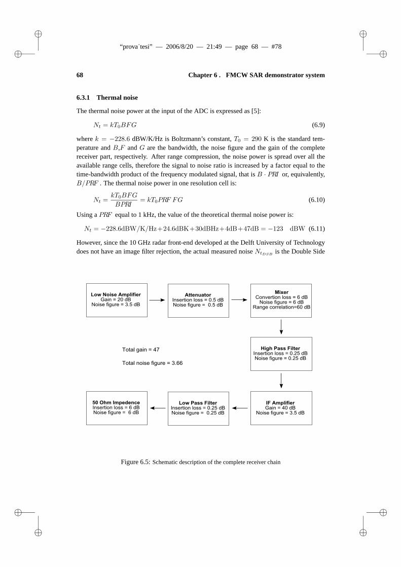
“prova˙tesi” — 2006/8/20 — 21:49 — page 68 — #78�

�

�

�

�

�

�

�


6.3.1 Thermal noise

The thermal noise power at the input of the ADC is expressed as [5]:

Nt = kT0BFG (6.9)

where k = −228.6 dBW/K/Hz is Boltzmann’s constant, T0 = 290 K is the standard tem-perature and B,F and G are the bandwidth, the noise figure and the gain of the completereceiver part, respectively. After range compression, the noise power is spread over all theavailable range cells, therefore the signal to noise ratio is increased by a factor equal to thetime-bandwidth product of the frequency modulated signal, that is B · PRI or, equivalently,B/PRF . The thermal noise power in one resolution cell is:

Nt =kT0BFG

BPRI= kT0PRF FG (6.10)

Using a PRF equal to 1 kHz, the value of the theoretical thermal noise power is:

Nt = −228.6dBW/K/Hz+24.6dBK+30dBHz+4dB+47dB = −123 dBW (6.11)

However, since the 10 GHz radar front-end developed at the Delft University of Technologydoes not have an image filter rejection, the actual measured noise NtDSB

is the Double Side

Figure 6.5: Schematic description of the complete receiver chain

“prova˙tesi” — 2006/8/20 — 21:49 — page 69 — #79�

�

�

�

�

�

�

�

6.3 Noise power calculation 69

Band (DSB), therefore 3 dB have to be added to the previous calculated value:

NtDSB= −120 dBW (6.12)

6.3.2 Phase noise

Because the front-end has two different antennas for the transmitting and the receiving part,the major contribution of the phase noise is determined by the coupling of the mixer. Thephase noise power related to the coupling of the mixer is [6]:

Np1 =PLONosc(fofs)

χ(6.13)

where PLO is the Local Oscillator (LO) signal power, Nosc is the oscillator phase noise at afrequency offset fofs relative to the carrier frequency and χ is the mixer isolation betweenthe RF and LO input signal. The phase noise is reduced due to the range correlation effect ifa fraction of the transmitted signal is used as LO signal [7]. The range correlation factor isequal to:

K2 = 4 sin(πfofsΔtpn) = 4 sin(πfofs2ΔRpn

c) (6.14)

in which Δtpn and ΔRpn are the time delay and the path of the mixer coupling. In fig. 6.6the range correlation factor is plotted as function of the coupling path (for constant frequencyoffset) and of the offset frequency (for constant coupling path).

After amplification, sampling and range compression, assuming the oscillator phase noiseconstant in a frequency bandwidth equal to the PRF , the phase noise power in one resolutioncell is:

Np = Np1PRF K2Gm (6.15)

0 5 10 15 20 25 30 35 40 45 50−90

−80

−70

−60

−50

−40

−30

Range − [cm]

Att

enua

tion

− [

dB]

Range correlation factor for fofs

= 1 MHz

0 0.5 1 1.5 2 2.5−120

−110

−100

−90

−80

−70

−60

−50

Frequency offset − [MHz]

Att

enua

tion

− [

dB]

Range correlation factor for ΔRpn

= 2 cm

Figure 6.6: Range correlation factor for the phase noise power as function of the path length (for aconstant frequency offset of 1 MHz) and of the frequency offset (for a constant path length of 2 cm).

“prova˙tesi” — 2006/8/20 — 21:49 — page 70 — #80�

�

�

�

�

�

�

�


where Gm is the gain of the receiver chain without the LNA, that is starting from the mixer.For the 10 GHz radar front-end, the following parameters hold for the calculation of thephase noise: PLO = -21 dBW, Nosc(1 MHz) = -113dBc/Hz, χ = -40dB, K2 ≈ -60dB (at 1MHz and assuming for the mixer a coupling path of 2 cm) and Gm = 27. Using (6.13) and(6.15) yields to:

Np = −21dBW − 113dBc/Hz − 40dB + 30dBHz − 60dB + 27dB

= −177 dBW (6.16)

For the final calculation, the same discussion done for the thermal noise holds for the phasenoise. The Double Side Band phase noise NpDSB

is 3 dB higher than the previously calcu-lated:

NpDSB= −174 dBW (6.17)

6.3.3 Quantization noise

The quantization noise can be expressed as:

Nq =q2

12(6.18)

where q is the quantization interval, and after range compression:

Nq =q2

12PRF

B(6.19)

The dynamic range of the system ADC is 0.4 Vpp and 12 bits are used (q = 0.4V/212), sofrom (6.19) the following value for the quantization noise in one resolution cell is obtained:

Nq = 2(−3.97 − 36.12) − 10.79 + 30 − 86.9 = −147.87 dBW (6.20)

6.3.4 Total noise

Combining (6.11), (6.16) and (6.20), the total noise power in one resolution cell, after sam-pling of the IF signal and range compression, equals to:

Ntot = NpDSB+ NpDSB

+ Nq ≈ −120dBW = −90 dBmW (6.21)

6.4 Experimental tests

Several tests and measurements have been carried out in order to verify the consistency ofthe front-end model previously developed. In the following subsections, laboratory measure-ments of the noise level and phase stability are reported.

“prova˙tesi” — 2006/8/20 — 21:49 — page 71 — #81�

�

�

�

�

�

�

�

6.5 Summary 71

6.4.1 Noise laboratory measurements

A measurement of the total system noise power Ntot with the transmitting antenna switchedoff has been performed. In this configuration only the noise and the delay line responsecontribute to the range profile. The results are presented in fig. 6.7; no windowing has beenapplied. The measurements show a noise level around -87.5 dB, a value very close to theexpected for the total noise power. The measured difference is around 2.5 dB. Also the delayline peak response, around -59 dB, matches very well the predicted power.

0 0.5 1 1.5 2 2.5−140

−130

−120

−110

−100

−90

−80

−70

−60

−50

−40Noise measurement, single pulse

Frequency − [MHz]

Abs

olut

e po

wer

− [

dBm

]

0 0.5 1 1.5 2 2.5−140

−130

−120

−110

−100

−90

−80

−70

−60

−50

−40Noise measurement, average power

Frequency − [MHz]

Abs

olut

e po

wer

− [

dBm

]

Figure 6.7: Noise power measurement results, with the delay line response present. In (a) a singleprocessed sweep is shown, while (b) presents the response after incoherent averaging of 1024 sweeps,corresponding to 1 second of data acquisition.

6.4.2 Phase measurements

A phase stability analysis has been performed on the collected data observing the behavior ofthe phase of the delay line response from sweep to sweep. Results are shown in fig. 6.8. Thestandard deviation of the phase has been calculated and corresponds to 0.119 radians. Addi-tionally, measurements with the 1 MHz filtering removed have been performed and reportedin the figure, where a slight phase degradation is noticeable.

6.5 Summary

The chapter has described the complete FMCW SAR system developed at the IRCTR, DelftUniversity of Technology. Particularly, a detailed analysis of the 10 GHz radar front-end, de-veloped within the work of this thesis, has been provided. Noise power calculations, based onthe schematic chain of the front-end, correspond very well with the laboratory measurements.

“prova˙tesi” — 2006/8/20 — 21:49 — page 72 — #82�

�

�

�

�

�

�

�

72 REFERENCES

0 0.5 1 1.5 2−4

−3

−2

−1

0

1

2

3

4Phase stability (0.11966), 1 MHz filter

Time − [s]

Pha

se −

[ra

d]

0 0.5 1 1.5 2−4

−3

−2

−1

0

1

2

3

4Phase stability (0.14809), no filter

Time − [s]

Pha

se −

[ra

d]

Figure 6.8: Filter effects on the phase stability.

References

[1] J. J. M. de Wit, Development of an Airborne Ka-Band FM-CW Synthetic Aperture Radar.Delft University of Technology, Ph. D. thesis, 2005.

[2] J. J. M. de Wit and P. Hoogeboom, “High-Rresolution Airborne FM-CW SAR: Designand Processing Aspects,” in Proc. European Conf. Synthetic Aperture Radar EUSAR’02,Cologne, Germany, June 2002, pp. 163–166.

[3] J. F. M. Lorga, A. Meta, J. J. M. de Wit, P. Hoogeboom, and J. A. Mulder, “AirborneFM-CW SAR and Integrated Navigation System Data Fusion,” in Proc. AIAA Guidance,Navigation, Control Conf. GNC’05, San Francisco, USA, Aug. 2005, pp. 201–205.

[4] D. Kalloemisier, Remote Control Software voor de FM-CW SAR Demonstrator. TUDelft - IRCTR, Tech. Rep. IRCTR-SH-013-03, 2003.


[6] W. P. Robins, Phase Noise in Signal Sources. Peter Peregrinus, London, 1982.

[7] M. C. Budge and M. P. Burt, “Range Correlation Effects in Radar,” in Proc. IEEE Nat.Radar Conf. ’93, Lynnfield, USA, Apr. 1993, pp. 212–216.

“prova˙tesi” — 2006/8/20 — 21:49 — page 73 — #83�

�

�

�

�

�

�

�

73

Chapter 7

Flight test campaign results

The chapter presents an overview of the FMCW SAR flight test campaign organized during the last

part of 2005 and the results obtained. Thanks to the special algorithms which have been developed

during the research project and described in the previous chapters, FMCW SAR images with a measured

resolution up to 45 cm times 25 cm (including Hamming windowing) were produced. Several tests

performed during the flight campaign (imaging at different resolutions, varying the incident angle, MTI

experiment) are reported and discussed. For the first time, high resolution SAR images have been

produced with an FMCW radar based on a simple VCO technology and the outstanding improvements

achievable with the invented frequency non-linearity correction algorithm have been demonstrated with

real data.

7.1 Introduction

An airborne flight test campaign has been organized and carried out in October 2005, at theStrausberg airport, east of Berlin. The aim of the campaign was to show the practicability ofan FMCW SAR and provide images of high resolution. The data acquired are of very highinterest: they represent one of the very first FMCW SAR data collection and have been usedto verify the developed algorithms on real data.

The 10 GHz FMCW SAR demonstrator system developed and built at the IRCTR, DelftUniversity of Technology, and described in the previous chapter, was brought to Strausbergwhere Stemme GmbH is located. The company was asked to provided the S10 light motorglider used for the flight test campaign. The particular aircraft was chosen because it couldprovide the means to prove that an airborne FMCW SAR can be operated with such a kind ofcarrier and because it was a very relatively cheap test aircraft.

Several runs were flown over the Strausberg urban area and rural fields. Different inci-dent angles, resolution and altitude configuration were tried; some tests illuminating a high-way were performed in order to validate MTI algorithms and the FMCW SAR model. Theflight campaign was very successful [1]. The following sections report FMCW SAR im-ages obtained processing the data collected during the campaign, resolution performance andcomparison with optical pictures. The algorithms described in the previous chapters have

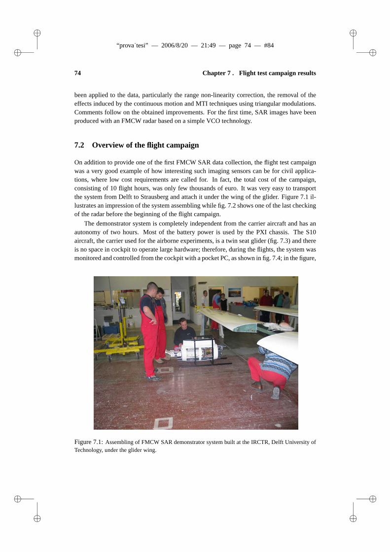
“prova˙tesi” — 2006/8/20 — 21:49 — page 74 — #84�

�

�

�

�

�

�

�

74 Chapter 7 . Flight test campaign results

been applied to the data, particularly the range non-linearity correction, the removal of theeffects induced by the continuous motion and MTI techniques using triangular modulations.Comments follow on the obtained improvements. For the first time, SAR images have beenproduced with an FMCW radar based on a simple VCO technology.

7.2 Overview of the flight campaign

On addition to provide one of the first FMCW SAR data collection, the flight test campaignwas a very good example of how interesting such imaging sensors can be for civil applica-tions, where low cost requirements are called for. In fact, the total cost of the campaign,consisting of 10 flight hours, was only few thousands of euro. It was very easy to transportthe system from Delft to Strausberg and attach it under the wing of the glider. Figure 7.1 il-lustrates an impression of the system assembling while fig. 7.2 shows one of the last checkingof the radar before the beginning of the flight campaign.

The demonstrator system is completely independent from the carrier aircraft and has anautonomy of two hours. Most of the battery power is used by the PXI chassis. The S10aircraft, the carrier used for the airborne experiments, is a twin seat glider (fig. 7.3) and thereis no space in cockpit to operate large hardware; therefore, during the flights, the system wasmonitored and controlled from the cockpit with a pocket PC, as shown in fig. 7.4; in the figure,

Figure 7.1: Assembling of FMCW SAR demonstrator system built at the IRCTR, Delft University ofTechnology, under the glider wing.

“prova˙tesi” — 2006/8/20 — 21:49 — page 75 — #85�

�

�

�

�

�

�

�

7.2 Overview of the flight campaign 75

Figure 7.2: Checking FMCW SAR demonstrator system.

the main power switch, used to turn the system and the radar front-end on and off, is alsovisible. Figure 7.5 shows a picture of the FMCW SAR pod taken from the cockpit during anoperational flight. During the flight stops, the system battery could be recharged; furthermore,additional checking and changing, i.e. varying the configuration antenna incident angle, couldbe performed very easily, see fig. 7.6.

In the flight test campaign, no motion sensors were installed in the demonstrator system,therefore the SAR images reported in this chapter have been obtained applying autofocusingtechniques. Hamming windowing is used both in range and in azimuth in order to reduce thesidelobe levels, at the cost of a coarser resolution.

“prova˙tesi” — 2006/8/20 — 21:49 — page 76 — #86�

�

�

�

�

�

�

�


Figure 7.3: Preparation for one flight with the twin seat S10 motor glider.

Figure 7.4: The Pocket PC used to control the FMCW SAR demonstrator system and the main switchare visible.

“prova˙tesi” — 2006/8/20 — 21:49 — page 77 — #87�

�

�

�

�

�

�

�

7.2 Overview of the flight campaign 77

Figure 7.5: FMCW SAR demonstrator system during one operational flight.

Figure 7.6: FMCW SAR demonstrator system during one flight stop. Battery charging and additionalchecking or changing could be easily performed.

“prova˙tesi” — 2006/8/20 — 21:49 — page 78 — #88�

�

�

�

�

�

�

�


7.3 Non-linearities correction

A novel and efficient processing technique for the frequency non-linearity correction has beenintroduced in chapter 3. It has been applied to the real data collected during the flight testcampaign resulting in outstanding improvements in the FMCW SAR images, both in termsof resolution and signal to noise ratio. Three representative examples are reported here.

7.3.1 First example

The first example is about results obtained with data collected during a flight with a mediumresolution configuration, transmitting a bandwidth of 260 MHz. The phase non-linearity esti-mation and the corresponding spectrum are shown in fig. 7.7, while fig. 7.8 illustrates the SARimages produced with and without frequency non-linearity correction. The improvements areclearly visible. In the lower-right part of the SAR images a bright scatterer response is visi-ble. The response of this point of opportunity is used to quantify the improvement achievedwith the non-linearity correction. Figure 7.9(a) shows the range profile obtained without thenon-linearity correction, while results obtained with the correction applied are reported infig. 7.9(b). The peak level increases of almost 7 dB while the integrated sidelobe level (ISL)improves of approximately 9.2 dB. The ISL shall here mean the square root of the ratio of theintegrated sidelobe power (ISP) of the response to the power in the main lobe of the response.Since the analyzed response is the echo of a point of opportunity, the integrated power con-tained in an area of three resolution cells around the maximum peak has been used as mainlobe power. The results of the analysis are summarized in tab. 7.1.

−6 −4 −2 0 2 4 6

x 10−4

0

5000

10000

15000

Time − [ms]

Phas

e −

[ra

d]

−1.5 −1 −0.5 0 0.5 1 1.5−20

−10

0

10

20

30

40

50

Beat frequency − [MHz]

Nor

mal

ized

am

plitu

de −

[dB

]

Figure 7.7: First example. Phase of the estimated non-linearity and corresponding spectrum.

“prova˙tesi” — 2006/8/20 — 21:49 — page 79 — #89�

�

�

�

�

�

�

�

7.3 Non-linearities correction 79

Figure 7.8: First example. Results of the non-linearity correction algorithm applied to FMCW SARdata collected with the medium resolution configuration. Slant range is on the vertical axis.

“prova˙tesi” — 2006/8/20 — 21:49 — page 80 — #90�

�

�

�

�

�

�

�


620 630 640 650 660 670 680 690 70030

40

50

60

70

80

90

Nor

mal

ized

am

plitu

de −

[dB

]

Slant range − [m]

(a)

620 630 640 650 660 670 680 690 70030

40

50

60

70

80

90

Nor

mal

ized

am

plitu

de −

[dB

]

Slant range − [m]

(b)

Figure 7.9: First example. Range profiles of a point of opportunity visible in the lower-right part of theSAR image shown in fig. 7.8: in (a) without the non-linearity correction and in (b) with the correction.An increased peak level and an improved integrated sidelobe level can be noticed.

Table 7.1: Results for the point of opportunity analysis.

without correction with correction

Peak level [dB] 77.62 84.40

ISP [dB] 86.95 71.90

ISL [dB] 2.72 -6.40

Range resolution at -3 dB [m] 1.2 1.2

Range resolution at - 10 db [m] 17 3.7

“prova˙tesi” — 2006/8/20 — 21:49 — page 81 — #91�

�

�

�

�

�

�

�


7.3.2 Second example

The second example is about data collected one hour later than the case described in theprevious example, with exactly the same configuration. However, from fig. 7.10, it is possibleto see that the estimated non-linearity spectrum is different from the one reported in fig. 7.7.The external conditions changed within one hour. Figure 7.11 shows the improvements onthe SAR image due to the frequency non-linearity correction.

−6 −4 −2 0 2 4 6

x 10−4

−2

−1.8

−1.6

−1.4

−1.2

−1

−0.8

−0.6

−0.4

−0.2

0x 10

4

Time − [ms]

Phas

e −

[ra

d]

−1.5 −1 −0.5 0 0.5 1 1.5−10

0

10

20

30

40

50


Nor

mal

ized

am

plitu

de −

[dB

]

Figure 7.10: Second example. Phase of the estimated non-linearity and corresponding spectrum.

“prova˙tesi” — 2006/8/20 — 21:49 — page 82 — #92�

�

�

�

�

�

�

�


Figure 7.11: Second example. Results of the non-linearity correction algorithm applied to FMCWSAR data collected with the medium resolution configuration. Slant range is on the vertical axis.

“prova˙tesi” — 2006/8/20 — 21:49 — page 83 — #93�

�

�

�

�

�

�

�


7.3.3 Third example

The last example reports the non-linearity estimation (fig. 7.7) and the effects of its correctionon the SAR image (fig. 7.11) collected over a forest area with a low resolution configurationwith a transmitted bandwidth of 130 MHz and PRI of 0.5 ms. Since the non-linearities areestimated from a delay line embedded in the front-end, it is not necessary to have point targetresponses in the SAR image.

The three examples demonstrate that the non-linearity has to be estimated for every datafile, because even small changes in external conditions can drastically affect the behavior ofthe VCO.

−3 −2 −1 0 1 2 3 4

x 10−4

−1800

−1600

−1400

−1200

−1000

−800

−600

−400

−200

0

200

Time − [ms]

Phas

e −

[ra

d]

−1.5 −1 −0.5 0 0.5 1 1.5−20

−10

0

10

20

30

40

50


Nor

mal

ized

am

plitu

de −

[dB

]

Figure 7.12: Third example. Phase of the estimated non-linearity and corresponding spectrum.

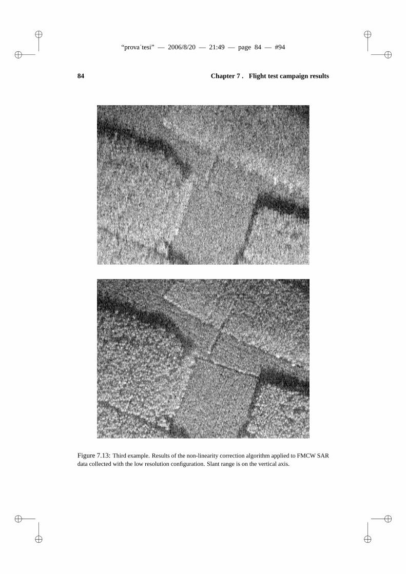
“prova˙tesi” — 2006/8/20 — 21:49 — page 84 — #94�

�

�

�

�

�

�

�


Figure 7.13: Third example. Results of the non-linearity correction algorithm applied to FMCW SARdata collected with the low resolution configuration. Slant range is on the vertical axis.

“prova˙tesi” — 2006/8/20 — 21:49 — page 85 — #95�

�

�

�

�

�

�

�

7.4 High resolution images 85

7.4 High resolution images

Some data at high resolution have been collected during a flight over the area near the Straus-berg airport with the following flight and radar configuration:

altitude 240 m;

incident angle 55o;

Range bandwidth 520 MHz;

Pulse duration 1 ms;

Maximum range 721 m.

Two images are reproduced in fig. 7.14 and fig. 7.15. After non-linearity correction, theprocessed SAR bandwidth has been set to 200 Hz, and an averaging of 16 cells in the crossdirection has been performed in order to reduce the speckle. In fig. 7.15, the response of acorner reflector is visible belove the crossing-roads. The resolution profiles are reported infig. 7.16, which show an obtained resolution of 45 cm in slant range times 25 cm in cross-range. The slant range resolution is slightly poorer than the theoretical 30 cm mainly becauseof Hamming windowing which reduces the sidelobe level to -40 dB but also introduces aresolution degradation of approximately a factor of 1.5.

Figure 7.14: High resolution image.

“prova˙tesi” — 2006/8/20 — 21:49 — page 86 — #96�

�

�

�

�

�

�

�



35536036537037538038539030

40

50

60

70

80

90

Slant range − [m]

Nor

mal

ized

am

plitu

de −

[dB

]

1565157015751580158515901595160030

40

50

60

70

80

90

Cross−range − [m]

Nor

mal

ized

am

plitu

de −

[dB

]

Figure 7.16: Range and cross-range profile of the corner reflector response in the high resolutionimage.

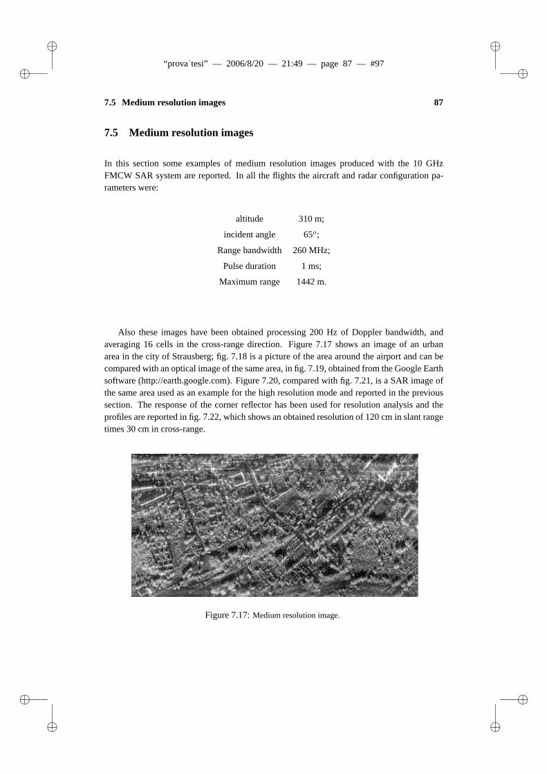
“prova˙tesi” — 2006/8/20 — 21:49 — page 87 — #97�

�

�

�

�

�

�

�

7.5 Medium resolution images 87

7.5 Medium resolution images

In this section some examples of medium resolution images produced with the 10 GHzFMCW SAR system are reported. In all the flights the aircraft and radar configuration pa-rameters were:

altitude 310 m;

incident angle 65o;


Pulse duration 1 ms;


Also these images have been obtained processing 200 Hz of Doppler bandwidth, andaveraging 16 cells in the cross-range direction. Figure 7.17 shows an image of an urbanarea in the city of Strausberg; fig. 7.18 is a picture of the area around the airport and can becompared with an optical image of the same area, in fig. 7.19, obtained from the Google Earthsoftware (http://earth.google.com). Figure 7.20, compared with fig. 7.21, is a SAR image ofthe same area used as an example for the high resolution mode and reported in the previoussection. The response of the corner reflector has been used for resolution analysis and theprofiles are reported in fig. 7.22, which shows an obtained resolution of 120 cm in slant rangetimes 30 cm in cross-range.

Figure 7.17: Medium resolution image.

“prova˙tesi” — 2006/8/20 — 21:49 — page 88 — #98�

�

�

�

�

�

�

�



Figure 7.19: Google image.

“prova˙tesi” — 2006/8/20 — 21:49 — page 89 — #99�

�

�

�

�

�

�

�

7.5 Medium resolution images 89



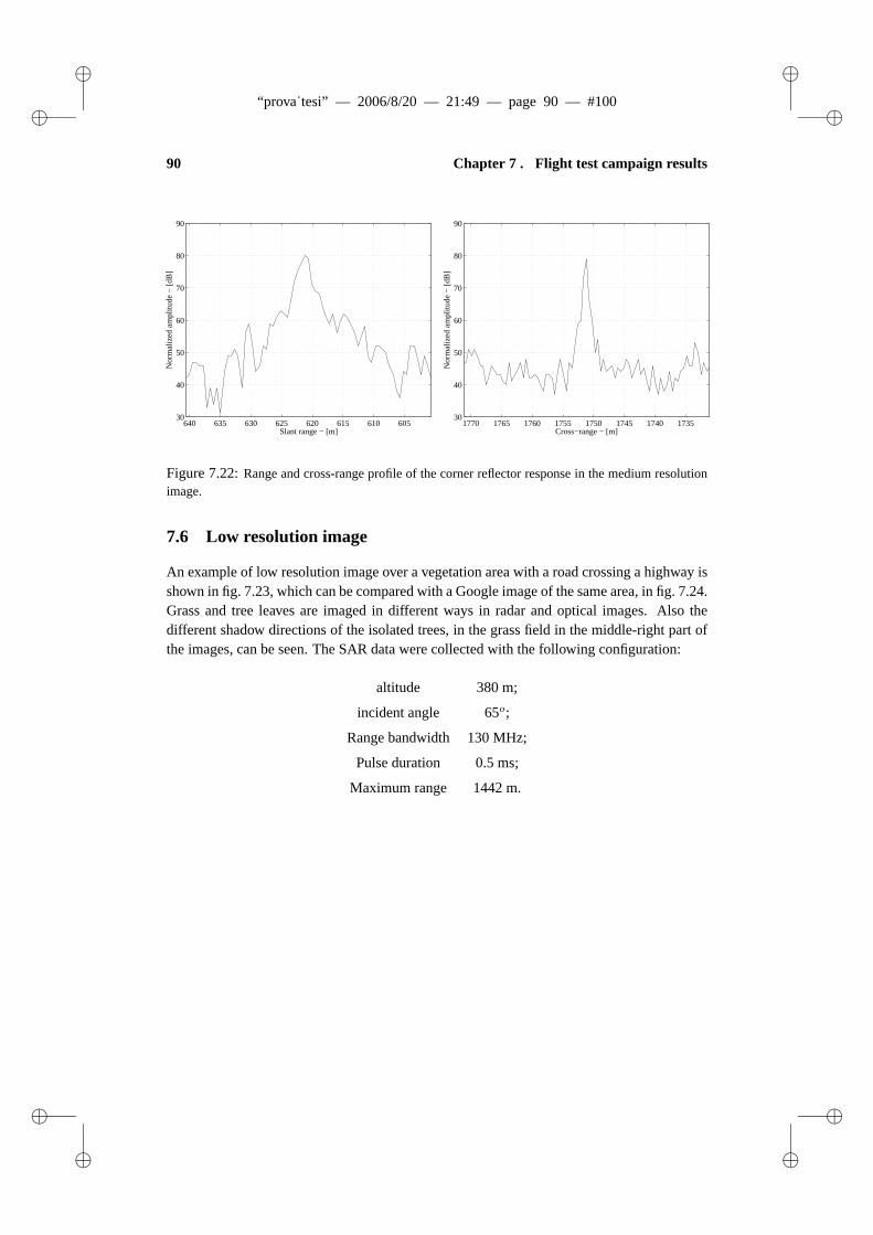
“prova˙tesi” — 2006/8/20 — 21:49 — page 90 — #100�

�

�

�

�

�

�

�


60561061562062563063564030

40

50

60

70

80

90

Slant range − [m]

Nor

mal

ized

am

plitu

de −

[dB

]

1735174017451750175517601765177030

40

50

60

70

80

90

Cross−range − [m]

Nor

mal

ized

am

plitu

de −

[dB

]

Figure 7.22: Range and cross-range profile of the corner reflector response in the medium resolutionimage.

7.6 Low resolution image

An example of low resolution image over a vegetation area with a road crossing a highway isshown in fig. 7.23, which can be compared with a Google image of the same area, in fig. 7.24.Grass and tree leaves are imaged in different ways in radar and optical images. Also thedifferent shadow directions of the isolated trees, in the grass field in the middle-right part ofthe images, can be seen. The SAR data were collected with the following configuration:

altitude 380 m;

incident angle 65o;


Pulse duration 0.5 ms;


“prova˙tesi” — 2006/8/20 — 21:49 — page 91 — #101�

�

�

�

�

�

�

�

7.6 Low resolution image 91

Figure 7.23: Low resolution image.


“prova˙tesi” — 2006/8/20 — 21:49 — page 92 — #102�

�

�

�

�

�

�

�


7.7 Resolution comparison

Several flights with different resolution configurations were flown over the same region aroundthe airport area. A close view of the SAR images on the same building area at low, mediumand high resolution is reported in fig. 7.25, fig. 7.26, fig. 7.27, respectively.

Figure 7.25: Low resolution image.

It can be seen how the details become clearer and sharper with increasing resolution.Finally, a corresponding optical image, taken from the glider cockpit with an optical cameraduring one of the flights, is shown in fig. 7.28. In the upper right corner of the image, parkedcars are visible. In the high resolution FMCW SAR image they are clearly detected anddiscriminated.

“prova˙tesi” — 2006/8/20 — 21:49 — page 93 — #103�

�

�

�

�

�

�

�

7.7 Resolution comparison 93


“prova˙tesi” — 2006/8/20 — 21:49 — page 94 — #104�

�

�

�

�

�

�

�



Figure 7.28: Optical camera image.

“prova˙tesi” — 2006/8/20 — 21:49 — page 95 — #105�

�

�

�

�

�

�

�

7.8 Triangular FMCW SAR test 95

7.8 Triangular FMCW SAR test

Data acquired transmitting a triangular modulation were used to verify the FMCW SARmodel developed in chapter 4 and the MTI algorithm using frequency slope diversity de-scribed in chapter 5. In triangular modulation, the frequency rate α of the upslope part isthe opposite of the downslope. If not corrected for, the motion within the sweep will haveopposite effects in the SAR images produced with the two different parts of the modulation,as described in (4.16), reformulated here exploiting the term α:

SIF (Kr,Kx) = exp (jKxvt) exp j(R

√K2

r − K2x − Kxx1

)

= exp(

jKxvKr − Krc

4πα

)exp j

(R

√K2

r − K2x − Kxx1

)(7.1)

After correction of the effects induced by the continuous motion within the sweep, thestationary clutter in the two images has to be imaged exactly in the same way if flying alongto a straight line. During this test, the radar was moving at around 33 m/s, the antenna aper-ture beamwidth was 20o, and the duration of the transmitted 130 MHz triangular modulationperiod 1 ms (half for the upslope and half for the downslope). Therefore, for each image,the value of K (introduced in chapter 4, (4.7)) is approximately equal to 0.4. The amplitudeimage obtained with the upslope part is illustrated in fig. 7.29.

Figure 7.29: Results of the flight test transmitting 130 MHz triangular modulation showing the up-slope image amplitude where the part within the rectangular frame has been used for the subsequentinterferogram comparison.

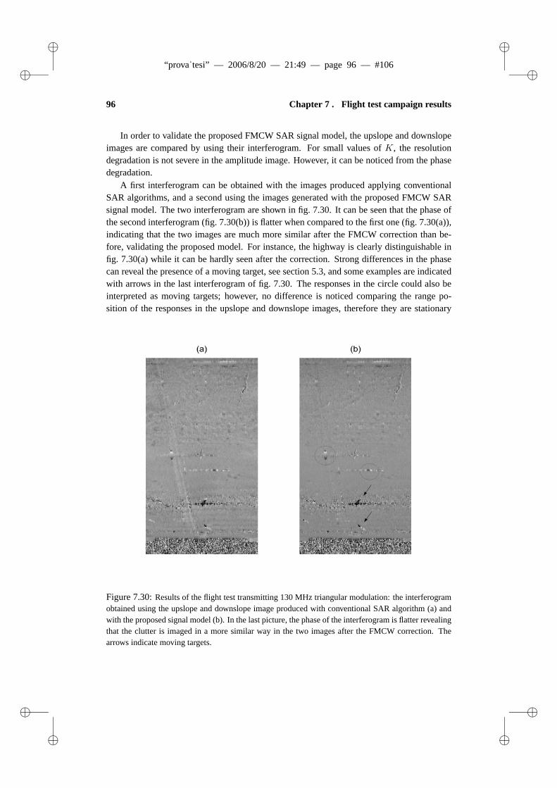
“prova˙tesi” — 2006/8/20 — 21:49 — page 96 — #106�

�

�

�

�

�

�

�


In order to validate the proposed FMCW SAR signal model, the upslope and downslopeimages are compared by using their interferogram. For small values of K, the resolutiondegradation is not severe in the amplitude image. However, it can be noticed from the phasedegradation.

A first interferogram can be obtained with the images produced applying conventionalSAR algorithms, and a second using the images generated with the proposed FMCW SARsignal model. The two interferogram are shown in fig. 7.30. It can be seen that the phase ofthe second interferogram (fig. 7.30(b)) is flatter when compared to the first one (fig. 7.30(a)),indicating that the two images are much more similar after the FMCW correction than be-fore, validating the proposed model. For instance, the highway is clearly distinguishable infig. 7.30(a) while it can be hardly seen after the correction. Strong differences in the phasecan reveal the presence of a moving target, see section 5.3, and some examples are indicatedwith arrows in the last interferogram of fig. 7.30. The responses in the circle could also beinterpreted as moving targets; however, no difference is noticed comparing the range po-sition of the responses in the upslope and downslope images, therefore they are stationary

Figure 7.30: Results of the flight test transmitting 130 MHz triangular modulation: the interferogramobtained using the upslope and downslope image produced with conventional SAR algorithm (a) andwith the proposed signal model (b). In the last picture, the phase of the interferogram is flatter revealingthat the clutter is imaged in a more similar way in the two images after the FMCW correction. Thearrows indicate moving targets.

“prova˙tesi” — 2006/8/20 — 21:49 — page 97 — #107�

�

�

�

�

�

�

�

7.8 Triangular FMCW SAR test 97

Figure 7.31: Schematic representation of the moving target experiment. The two cars are driving onthe highway.

targets. Additionally, this was confirmed by ground truth. The particular response of thesestrong stationary targets in the interferogram, similar to a moving target response, is due tothe fact that part of the processed target energy is coming from the antenna sidelobes. There-fore, the Doppler response of these stationary targets contains also energy folded back in theclutter bandwidth, which disturbs the phase response in the final SAR image. Remainingphase discrepancies could be due to a not completely exact motion compensation; in fact, thedemonstrator system was not provided with motion sensors and therefore the SAR process-ing relays entirely on autofocusing techniques, which can assure a good image focusing butcannot guarantee an accurate flight geometry reconstruction.

A quantitative analysis has been performed for the responses of the two moving targetsindicated with an arrow in fig. 7.30 in order to calculate their velocity. The PRF ambiguityhas been resolved measuring the range displacement nv , in terms of resolution cells, of theresponse in the upslope and downslope FMCW SAR images. The Doppler frequency of thetarget is finally obtained using also the ambiguous Doppler information estimated from the

Table 7.2: Results for the moving target analysis.

target 1 target 2

Slant range [m] 450 540

Ground range [m] 241 383

Elevation angle [o] 32.4 45.3

nv 1 1

Measured Doppler [Hz] -200 100

Target Doppler [Hz] 800 1100

Ground velocity [km/h] 82.4 85.4

“prova˙tesi” — 2006/8/20 — 21:49 — page 98 — #108�

�

�

�

�

�

�

�

98 REFERENCES

spectrum response. An inclination of 12o between the highway and the cross track directionhas been assumed, as shown in fig. 7.8, for the calculation of the target ground velocity. Theresults of the analysis are consistent with the illuminated scenario and are reported in tab. 7.2.

7.9 Summary

The chapter has presented an overview of the FMCW SAR flight test campaign organized dur-ing the last part of 2005 and the results obtained. Thanks to the special algorithms which havebeen developed during the research project and described in the previous chapters, FMCWSAR images with a measured resolution up to 45 cm times 25 cm (including Hamming win-dowing) were obtained. During the campaign, the system was not provided with motionsensors therefore a complete motion compensation has not be performed. The SAR process-ing relied on autofocusing techniques which can achieve a good cross-range focusing.

Several tests performed during the flight campaign (imaging at different resolutions,varying the incident angle, triangular modulation experiment for MTI and validation of theFMCW SAR model) are reported and discussed. For the first time, SAR images have beenproduced with an FMCW radar based on a simple VCO technology and the outstanding im-provements achievable with the invented frequency non-linearities correction algorithm havebeen demonstrated with real data.

References

[1] A. Meta, P. Hakkaart, F. V. der Zwan, P. Hoogeboom, and L. P. Ligthart, “First demonstra-tion of an X-band airborne FMCW SAR,” in Proc. European Conf. on Synthetic ApertureRadar EUSAR’06, Dresden, Germany, May 2006.

“prova˙tesi” — 2006/8/20 — 21:49 — page 99 — #109�

�

�

�

�

�

�

�

99

Chapter 8

Conclusions and discussion

Synthetic Aperture Radar is very successfully used in many earth observation applications.Operating existing SAR systems, however, are quite costly, which makes them an unlikelychoice for extensive applications requiring frequent revisits. Additionally, their use is prob-lematic in many military tasks where very compact and lightweight high-resolution imagingsystems are required, which can operate independently of the weather conditions and sunillumination.

The combination of FMCW technology and SAR techniques offers a solution to the in-creasing request for low cost, compact imaging sensors with high resolution. FMCW radarsoperate with a low transmission power and their raw data bandwidth is drastically reduced ascompared to conventional SAR systems.

With the work described in the thesis, the practical feasibility of an airborne FMCW SARhas been demonstrated. Algorithms for the proper processing of FMCW SAR data, whichresult in outstanding improvements when compared with conventional methods, allowed theuse of very simple and cheap technology. The contents of this thesis represent an importantcontribution to the development of compact, low cost imaging sensors with high resolution.The author aimed to provide the scientific community with a complete and detailed analysisof the FMCW SAR signal and the proper tools to process it.

8.1 Contributions of this research

Within the framework of the project, the following novelties and main results have beenreached and have been presented in the thesis:

Non-linearity correction. A novel processing solution, which completely solves the prob-lem of the presence of frequency non-linearities in FMCW SAR, has been invented. It cor-rects the non-linearity effects for the whole range profile at once, and it allows a perfectrange focussing. The proposed method operates directly on the deramped data and it is verycomputationally efficient [1].

A complete FMCW SAR signal model. A detailed analytical description for the FMCWSAR signal in the two-dimensional frequency domain has been presented. Based on this

“prova˙tesi” — 2006/8/20 — 21:49 — page 100 — #110�

�

�

�

�

�

�

�

100 Chapter 8 . Conclusions and discussion

model, proper algorithms have been developed which guarantee the best performance whenprocessing FMCW SAR data. The results of their use on real data proved their validity [2].

MTI with frequency modulated CW SAR. Two SAR MTI methods are proposed. Thefirst is based on the frequency slope diversity in the transmitted modulation by using lineartriangular FMCW SAR [3]. The second makes use of the Doppler filtering properties ofrandomized SFCW modulations [4].

First demonstration of an X-band FMCW SAR. A flight campaign has been organizedduring the last part of 2005 to test the 10 GHz FMCW radar front-end developed at theIRCTR. The feasibility of an operational FMCW SAR under practical circumstances hasbeen demonstrated and one of the very first FMCW SAR data collection has been acquired.The results were very successful. Thanks to the special algorithms developed, high resolutionFMCW SAR images have been obtained for the first time using a simple front-end based oncheap FMCW technology [5].

8.2 Recommendations

The development of new algorithms for the proper processing of FMCW SAR data and apractical implementation of an FMCW SAR system have been presented in the thesis. Duringthe research stage, a number of new problems have been identified, which require furtherstudies. A list of new directions to be investigated include:

• evaluation of the robustness of the SAR MTI algorithm based on triangular FMCWpresented in section 5.3.

• validation with real data of the proposed deramping technique described in section 3.6.1and of the MTI applications of the randomized SFCW signals proposed in section 5.4.

• investigation of the use of DDS technology for randomized SFCW signals and, in gen-eral, for CW noise radars. DDS can offer a great versatility for many signal processingtechniques which require high precise deterministic waveforms.

• study of a bistatic dechirp-on-receive FMCW SAR configuration. Having a receivingantenna on a separate carrier can eliminate the constraint of limited maximum rangein conventional monostatic FMCW radar, imposed by the coupling of transmitting andreceiving chain.

• analysis of adaptive FMCW waveforms for in-flight autofocusing. For instance, thecommonly used adaptation of the PRF to account for along track velocity errors inconventional SAR involves a change of the frequency rate in FMCW sensors, if aconstant transmitted bandwidth is wanted. An adapted version of the non-linearitycorrection algorithm described in chapter 3 could be used.

“prova˙tesi” — 2006/8/20 — 21:49 — page 101 — #111�

�

�

�

�

�

�

�

8.3 Related works at other institutes 101

8.3 Related works at other institutes

That FMCW SAR will play an in increasing important role in future small, low-cost imagingradar applications is additionally demonstrated by the fact that, very recently, other instituteshave developed systems or started concept studies on SAR based on FMCW technology. Abrief description of them follows.

MISAR system [6]; it is a miniaturized FMCW SAR designed by EADS (European Aero-nautic Defence System) in Ulm, Germany. It can be carried by a small UAV. Raw data aretransmitted to the ground, with standard video links, where they are successively processed.The system operates at 35 GHz and produces images with a resolution up to 0.5 m x 0.5 m.

3D imaging radar ARTINO [7]; at FGAN (Forschungsgesellschaft fur Angewandte Natur-wissenschaften) in Wachtberg, Germany, a 3D FMCW radar concept is being developed un-der the name ARTINO. The main idea of the system is the use of a linear array of nadirpointing antennas for across-track imaging. It operates at Ka band and it is designed for UAVapplications.

BYU microSAR [8]; developed by Brigham Young University, USA, it is a low costFMCW SAR system intended for operations on a small UAV. Raw data are stored on acompact flash disk and processed off-line. The front-end operates at 5.4 GHz transmittinga bandwidth of 80 MHz and it irradiates 1 W power through a patch antenna.

ONERA 3D FMCW SAR [9]; similar to the ARTINO project, it is a 3D SAR for radarimagery being developed by ONERA, France. It also works at Ka band and is foreseen to bedeployed on a similar Stemme motor glider as the one used for the TU Delft FMCW SARflight test campaign.

References


[2] A. Meta, P. Hoogebbom, and L. P. Ligthart, “Correction of the effects induced by thecontinuous motion in FMCW SAR,” in Proc. IEEE Radar Conf. ’06, Verona, NY, USA,Apr. 2006, pp. 358–365.


[4] A. Meta, P. Hoogeboom, and L. P. Ligthart, “Moving Target Indication enhancement inFMCW SAR using deramped randomized stepped-frequency signals,” in Proc. WaveformDiversity and Design Conf. WDDC’06, Lihue, HI, USA, Jan. 2006.

“prova˙tesi” — 2006/8/20 — 21:49 — page 102 — #112�

�

�

�

�

�

�

�

102 REFERENCES

[5] A. Meta, P. Hakkaart, F. V. der Zwan, P. Hoogeboom, and L. P. Ligthart, “First demonstra-tion of an X-band airborne FMCW SAR,” in Proc. European Conf. on Synthetic ApertureRadar EUSAR’06, Dresden, Germany, May 2006.

[6] M. Edrich, “Design Overview and Flight Test Results of the Miniaturised SAR SensorMISAR,” in Proc. EuRAD’04, Amsterdam, The Netherlands, Oct. 2004, pp. 205–208.

[7] M. Weiss and J. Ender, “A 3d imaging radar for small unmanned airplanes - ARTINO,”in Proc. EuRAD’05, Paris, France, Oct. 2005, pp. 229–232.

[8] E. Zaugg, D. Hudson, and D. Long, “The BYU mSAR: a small, student-built for UAV op-eration,” in Proc. IEEE Int. Geoscience and Remote Sensing Symp. IGARSS’06, Denver,USA, July 2006.

[9] R. Giret, H. Jeuland, and P. Enert, “A study ofa 3D-SAR concept for a millimiter-waveimaging radar onboard an UAV,” in Proc. EuRAD’04, Amsterdam, The Netherlands, Oct.2004, pp. 201–204.

“prova˙tesi” — 2006/8/20 — 21:49 — page 103 — #113�

�

�

�

�

�

�

�

103

Appendix A

Non-linear Frequency Scaling Algorithm forFMCW SAR data

This appendix presents a novel approach for processing data acquired with FMCW dechirp-on-receive

systems by using a non-linear frequency scaling algorithm. The presented material is taken from [1].

The range frequency non-linearity correction, the Doppler shift induced by the continuous motion and

the range migration removal are performed in the same step in the wavenumber domain with an efficient

solution. The cross-range focusing is then achieved with conventional matched filtering.

A.1 Introduction

FMCW sensors can continuously transmit linear chirps, and the use of dechirp-on-receiveconfigurations allows an high reduction of the sampling frequency. As described in chapter 3non-linearities deteriorate the range resolution when deramping techniques are used becausethey spread the target energy through different frequencies.

For the processing of SAR data, several algorithms have been developed and each ofthem has different characteristics which make them appropriate for different applications.Particularly, the frequency scaling algorithm (FSA) can process deramped data [2] and it isable to correct the range migration without using interpolations.

The novel approach presented in the appendix aims to combine the non-linearity correc-tion, developed by the author within the framework of the thesis, the FSA and the removalof the FMCW Doppler shift. Both non-linearity correction and FSA are based on residualvideo phase removal, therefore this property can be exploited to integrate the algorithms anddecrease the, already low, computational load. The result is the non-linear frequency scalingalgorithm, which is presented in this appendix. It has a computational load nearly equal to theconventional method, with the advantage of additionally correcting the Doppler shift effectinduced by the continuous motion and the frequency non-linearity degradation. Therefore,the proposed algorithm is very suitable for the processing of FMCW SAR data.

The remaining of the appendix is structured in three sections. Section A.2 derives thewavenumber domain deramped FMCW signal taking into account the range frequency non-

“prova˙tesi” — 2006/8/20 — 21:49 — page 104 — #114�

�

�

�

�

�

�

�

104 Appendix A . Non-linear Frequency Scaling Algorithm for FMCW SAR data

linearities and without using the stop-and-go approximation. Next, the combination of theFMCW Doppler shift, frequency non-linearity and range migration correction is described insection A.3. Finally, conclusions are stated in section A.4.

A.2 Deramped non-linear FMCW SAR signal

This section derives an analytical description of the deramped FMCW SAR signal in thetwo-dimensional frequency domain including the range frequency non-linearities and with-out using the stop-and-go approximation. The radar continuously transmits linear FM chirpshaving duration Tp equal to the pulse repetition interval PRI , chirp rate α = B/PRI , whereB is the transmitted bandwidth and center frequency fc. The transmitted frequency is ex-pressed as:

fr = fc + αt + e(t) (A.1)

where −PRI/2 ≤ t < PRI/2 and e(t) is the frequency non-linearity term, which is un-wanted. In dechirp-on-receive systems, the received and transmitted signal are mixed inorder to reduce the required system sampling rate. In a stripmap configuration with the radarflying along a straight path, the target time delay is:

τ =2c

√R2 + v2(t + T )2 (A.2)

where R is the distance of closest approach, v is the aircraft velocity and T is the slow timevariable. The deramped FMCW SAR signal can be described by:

s(t, T ) = exp(−j2π(fcτ + ατt − 12ατ2 + e(t) − e(t − τ))) (A.3)

The first exponential term is the azimuth phase history; the second term is the range signalwhile the third term is the residual video phase. The last two terms of (A.3) represent theunwanted contribution of the frequency non-linearities; e(t) can be directly measured or es-timated from the raw data [3] and is assumed known in the rest of the analysis. Frequencynon-linearities seriously degrade the system performances if not corrected for. Applying aFourier transform with respect to the variable T to (A.3), and after developing the calcula-tions, the signal in the range-Doppler domain can be expressed as:

s(t, fD) ≈(

exp[−j

4πRβ(fD)λ

]exp

[−j

4παR

cβ(fD)t

]

exp(j2πfDt) exp[j

(e(t) − e

(t − 2R

cβ(fD)

))]

src(t, fD;R))∗ exp(−jπαt2) (A.4)

where ∗ represents the convolution operation. Differently from [2], the expression in (A.4) in-cludes the non-linearity and the Doppler shift terms The Doppler frequency fD varies within:

−PRF

2+ fDc ≤ fD ≤ PRF

2+ fDc (A.5)

“prova˙tesi” — 2006/8/20 — 21:49 — page 105 — #115�

�

�

�

�

�

�

�

A.2 Deramped non-linear FMCW SAR signal 105

where PRF is the pulse repetition frequency and fDc is the Doppler centroid. The first twoterms of (A.4) represent the azimuth phase history and the range modulation. The factorβ(fD) describes the range cell migration as a function of the Doppler frequency:

β(fD) =

√1 − f2

Dλ2

4v2(A.6)

The third and fourth terms are the consequences of the continuous motion within the sweep,which introduces a Doppler shift, and of the presence of range frequency non-linearities. Themodified non-linear frequency scaling algorithm differs from its conventional method for theability to remove the effects of the aforementioned two terms.

The src(t, fD;R) term in (A.4) is the secondary range compression and its expressioncan be found in [2], for instance.

Figure A.1: Schematic representation of the non-linear frequency scaling algorithm. 1) raw dataof three point scatterers. 2) Frequency scaling, Doppler shift, and transmitted non-linearity referencefunction. 3) Signal data after the multiply with the first reference function. 4) Residual video phasecorrection function. 5) Signal data after residual video phase correction. 6) Removal of the spreadinginduced by the frequency scaling and by the received non-linearity. 7) Signal after complete non-linearfrequency scaling. Range time is on the horizontal axis whereas vertical axes represent range frequency.In 2) and 6) dashed curves indicate the dependency on the Doppler frequency.

“prova˙tesi” — 2006/8/20 — 21:49 — page 106 — #116�

�

�

�

�

�

�

�

106 Appendix A . Non-linear Frequency Scaling Algorithm for FMCW SAR data

A.3 Frequency non-linearity, Doppler shift and range cell migrationcorrection

The non-linearity and RCM removal are obtained through the exploitation of the residualvideo phase. The two corrections are achieved at the same step. In fact, the frequency scalingcan be thought as a special case of frequency non-linearity correction, namely a linear case.Additionally, also the Doppler shift effects, induced by the continuous motion within thesweep, can be corrected at this stage.

The first step is a multiply of (A.4) with the following reference function:

H1(t, fD) = exp[−j(2πfDt + e(t) − παt2(1 − β(fD)))

](A.7)

which removes the Doppler shift, the transmitted non-linearity and scales the frequency. Suc-cessively, the signal is Fourier transformed with respect to t and multiplied with the RVPcorrection term:

H2(f, fD) = exp[−j

πf2

αβ(fD)

](A.8)

An inverse Fourier transform brings the signal back to the time domain:

s(t, fD) = exp[−j

4πRβ(fD)λ

]exp

[−j

4παR

ct

]

exp[−jπαt2(β(fD)2 − β(fD))

]exp [−jeRV P (t)] src(t, fD;R) (A.9)

where eRV P represents the non-linearity after it passed through the RVP filter. Finally, a lastreference function

H3(t, fD) = exp[jπαt2(β(fD)2 − β(fD))

]exp [jeRV P (t)] (A.10)

multiplies (A.9) removing the, now equalized, spreading of the peak response induced by thefrequency scaling and by the non-linearities. After this last step, the following expressiondescribes the resulting signal:

s(t, fD) = exp[−j

4πRβ(fD)λ

]exp

[−j

4παR

ct

]src(t, fD;R) (A.11)

At this point, conventional steps can be performed to achieve secondary range compressionand successively azimuth focusing. In the derivation, a reference range equal to zero hasbeen used; when needed, expressions with a different value of the reference range can be eas-ily derived. The proposed modified non-linear frequency scaling algorithm is very suitablefor the processing of FMCW SAR data. In fact, it corrects, with practically no additionalcomputational cost when compared with the conventional frequency scaling algorithm, theDoppler shift induced by the continuous motion in FMCW SAR and, particularly important,

“prova˙tesi” — 2006/8/20 — 21:49 — page 107 — #117�

�

�

�

�

�

�

�

A.4 Summary 107

the degradation caused by the frequency non-linearities. This last characteristic, in fact, al-lows the use of very simple and cheap sensors which can generate the transmitted modulationdirectly in the radio frequency band. A schematic representation of the algorithm is illus-trated in fig A.1. When applied to real data, the algorithm has produced similar images tothose presented in chapter 7 but with less computations.

A.4 Summary

This appendix has presented a modified non-linear frequency scaling algorithm for process-ing FMCW SAR data acquired with dechirp-on-receive systems. The range frequency non-linearity correction, the Doppler shift induced by the continuous motion and the range migra-tion removal are performed at the same step in the wavenumber domain with a very efficientsolution. The computational load of the described non-linear frequency scaling algorithm ispractically the same as the conventional one. Therefore, the proposed method is very suitablefor the processing of FMCW SAR data. The cross-range focusing is then performed withconventional matched filtering.

References

[1] A. Meta, P. Hoogeboom, and L. P. Ligthart, “Non-linear Frequency Scaling Algorithmfor FMCW SAR Data,” in Proc. EuRAD’06, Manchester, UK, Sep. 2006.

[2] J. Mittermayer, A. Moreira, and O. Loffeld, “Spotlight SAR Data Processing Using theFrequency Scaling Algorithm,” IEEE Trans. on Geoscience and Remote Sensing, vol. 37,no. 5, pp. 2198–2214, Sep. 1999.


“prova˙tesi” — 2006/8/20 — 21:49 — page 108 — #118�

�

�

�

�

�

�

�

108 REFERENCES

“prova˙tesi” — 2006/8/20 — 21:49 — page 109 — #119�

�

�

�

�

�

�

�

109

List of acronyms

ADC Analog to Digital ConverterDBF Digital Beam FormingCW Continuous WaveDAC Digital to Analog ConverterDDS Direct Digital SynthesizerDLR Deutsches Zentrum fur Luft-und Raumfahrt (German Aerospace Center)EADS European Aeronautic Defence and Space companyFFT Fast Fourier TransformFGAN Forschungsgesellschaft fur Angewandte Naturwissenschaften

(Research Establishment for Applied Science)FM Frequency ModulatedFMCW Frequency Modulated Continuous WaveFSA Frequency Scaling AlgorithmIF Intermediate FrequencyIRCTR International Research Centre for Telecommunications and RadarISL Integrated Sidelobe LevelISP Integrated Sidelobe PowerLNA Low Noise AmplifierLO Local OscillatorLPF Low Pass FilterLPI Low Probability of InterceptionMTI Moving Target IndicatorPRF Pulse Repetition FrequencyPRI Pulse Repetition IntervalRF Radio FrequencyRVP Residual Video PhaseSAR Synthetic Aperture RadarSAW Surface Acoustic WaveSFCW Stepped Frequency Continuous WaveSSNR Spreading to Sampling induced Noise RatioUAV Unmanned Aerial VehicleVCO Voltage Controlled Oscillator

“prova˙tesi” — 2006/8/20 — 21:49 — page 110 — #120�

�

�

�

�

�

�

�

110 List of acronyms

“prova˙tesi” — 2006/8/20 — 21:49 — page 111 — #121�

�

�

�

�

�

�

�

111

List of symbols

B transmitted bandwidthBD entire Doppler bandwidthBDi instantaneous Doppler bandwidthc speed of lightdi space one single antenna has moved during one sweepdN space between two adjacent subarray phase centere frequency non-linearityf frequencyfb beat frequencyfbmax

maximum beat frequencyfbmin

minimum beat frequencyfc carrier frequencyfD Doppler frequencyfDmax

maximum Doppler frequencyfDmin

minimum Doppler frequencyfn subpulse constant frequencyfr transmitted frequencyfs sampling frequencyfu unambiguous frequencyF . Fourier transform operatorF−1. Inverse Fourier transform operatorhnl VCO frequency non-linearity functionknj jitter noise factorK FMCW SAR parameterKc carrier range spatial frequencyKr range spatial frequencyKx cross-range spatial frequencyh flight heightlaz antenna length in the azimuth directionL SAR observation lengthnv number of range cell difference in triangular modulation MTIN subpulse number or number of antennas

“prova˙tesi” — 2006/8/20 — 21:49 — page 112 — #122�

�

�

�

�

�

�

�

112 List of symbols

r slant rangeR slant range of closest approachRu unambiguous ranges steering signalse steering correction signalsif intermediate frequency signalsif lin linear intermediate frequency signalslin steering signal producing a VCO linear outputst transmitted signalsε frequency non-linearity signalsε RV P frequency non-linearity signal after RVPt time within the pulseTp pulse durationTs subpulse durationx radar cross-range positionx1 cross-range coordinate of the scene centery1 range coordinate of the scene centerv aircraft velocityvr radial velocityα frequency sweep rateβ range migration factorγ look angleγmax maximum look angleγmin minimum look angleδaz azimuth resolutionδfb beat frequency resolutionδfr range frequency resolutionδr slant range resolutionδT slow time resolutionΔf frequency stepΔX azimuth displacement for moving targetΔXimag azimuth displacement for moving target in the SAR imagesΔR range displacement for moving target in the SAR imagesε non-linear error functionεif intermediate frequency non-linear error functionεRV P non-linear error function after RVP correctionε estimated non-linear error functionη duty cycleθ displacement slope of moving target in FMCW SAR imagesθaz azimuth 3-dB antenna beamwidthλ wavelengthλc carrier wavelength

“prova˙tesi” — 2006/8/20 — 21:49 — page 113 — #123�

�

�

�

�

�

�

�

113

μ oversampling factorξ instantaneous to entire Doppler bandwidth ratioρr range SAR resolutionρaz azimuth SAR resolutionτ time delayτref reference time delayτmax maximum time delayτmin minimum time delayτ0 constant time delayφn initial subpulse phaseχ(τ, fD) square root of the ambiguity function

“prova˙tesi” — 2006/8/20 — 21:49 — page 114 — #124�

�

�

�

�

�

�

�

114 List of symbols

“prova˙tesi” — 2006/8/20 — 21:49 — page 115 — #125�

�

�

�

�

�

�

�

115

Summary

In the field of airborne earth observation there is special attention to compact, cost effective,high resolution imaging sensors. Such sensors are foreseen to play an important role insmall-scale remote sensing applications, such as the monitoring of dikes, watercourses, orhighways. Furthermore, such sensors are of military interest; reconnaissance tasks could beperformed with small unmanned aerial vehicles (UAVs), reducing in this way the risk forone’s own troops.

In order to be operated from small, even unmanned, aircrafts, such systems must consumelittle power and be small enough to fulfill the usually strict payload requirements. Moreover,to be of interest for the civil market, cost effectiveness is mandatory.

Frequency Modulated Continuous Wave (FMCW) radar systems are generally compactand relatively cheap to purchase and to exploit. They consume little power and, due to thefact that they are continuously operating, they can transmit a modest power, which makesthem very interesting for military operations. Consequently, FMCW radar technology is ofinterest for civil and military airborne earth observation applications, specially in combinationwith high resolution Synthetic Aperture Radar (SAR) techniques. The novel combination ofFMCW technology and SAR techniques leads to the development of a small, lightweight andcost-effective high resolution imaging sensor.

SAR techniques have been successfully applied in combination with coherent pulse radars.Also the concept of synthetic aperture with FMCW sensors has already been put forward inliterature, and some experimental systems have been described. However, the practical fea-sibility of an airborne FMCW SAR was not evident; the experimental sensors described inliterature were, in fact, radars mounted on rail supports operating in ground SAR configura-tions and at short distances. The FMCW radars could perform measurements in each positionof the synthetic aperture and then be moved to the next one. As in conventional pulse SARsystems, the stop-and-go approximation could be used; such an approximation assumes theradar platform stationary during the transmission of the electromagnetic pulses and the re-ception of the corresponding echoes. For airborne FMCW radars, however, the stop-and-goapproximation can be not valid anymore because the platform is actually moving while con-tinuously transmitting. A complete model for the deramped FMCW SAR signal was missingin the literature.

In addition to the particular signal aspects relative to the combination of FMCW technol-ogy and SAR techniques, the use of FMCW radars for long range high resolution applications

“prova˙tesi” — 2006/8/20 — 21:49 — page 116 — #126�

�

�

�

�

�

�

�

116 Summary

was not evident. In practical FMCW sensors, specially when using cheap components, thepresence of unwanted non-linearities in the frequency modulation severely degrades the radarperformances for long distances. Again, proper processing methods to overcome such limi-tation due to frequency non-linearities were not available to the scientific community.

Therefore, the area of FMCW SAR airborne observation and related signal processingaspects was a very novel field of research. At the International Research Centre for Telecom-munications and Radar (IRCTR) of the Delft University of Technology, a project was initiatedto investigate the feasibility of FMCW SAR in the field of airborne earth observation and todevelop proper processing algorithms to fully exploit the capability of such sensors.

Within the framework of the project, the following novelties and main results have beenreached and are presented in the thesis:

Non-linearities correction. The author has developed a very novel processing solution,which completely solves the problem of the presence of frequency non-linearities in FMCWSAR. It corrects for the non-linearity effects for the whole range profile at once, and it allowsa perfect range focussing, independently of the looking angle. The proposed method operatesdirectly on the deramped data and it is very computationally efficient.

A complete FMCW SAR signal model. The author has proposed a detailed analyticalmodel for the FMCW SAR signal in the two-dimensional frequency domain. Based on thismodel, proper algorithms have been developed which guarantee the best performance whenprocessing FMCW SAR data.

Moving Target Indication (MTI) with frequency modulated CW SAR. Two SAR MTImethods are proposed. The first is based on the frequency slope diversity in the transmit-ted modulation by using linear triangular FMCW SAR, while the second makes use of theDoppler filtering properties of randomized SFCW modulations.

First demonstration of an X-band FMCW SAR. A flight test campaign has been organizedduring the last part of 2005. The results were very successful. The feasibility of an operationalFMCW SAR based on cheap components has been proved under practical circumstances.Thanks to the special algorithms developed, FMCW SAR images with a measured 45 cmtimes 25 cm resolution (including windowing) were obtained for the first time.

“prova˙tesi” — 2006/8/20 — 21:49 — page 117 — #127�

�

�

�

�

�

�

�

117

Samenvatting

In het veld van airborne aardobservatie is er bijzondere aandacht voor compacte, rendabele,hoge resolutie beeldvorming sensoren. Deze sensoren zullen in de toekomst een belangrijkerol spelen in kleine remote sensing toepassingen, zoals het controleren van dijken, waterwe-gen of snelwegen. Tevens zijn zulke sensoren interessant voor militaire doeleinden; verken-nings taken kunnen worden uitgevoerd met kleine onbemande vliegtuigen, hiermee wordt hetgevaar voor de eigen troepen verkleind.

Om het mogelijk te maken om zulke systemen te besturen vanuit kleine, zelfs onbemandevliegtuigen, moeten deze weinig energie verbruiken en klein genoeg zijn om aan de striktelaadvermogens eisen te voldoen. Tevens moet het rendabel zijn voor de niet-militaire markt.

Frequency Modulated Continuous Wave (FMCW) radar systemen zijn over het algemeencompact en betrekkelijk goedkoop om aan te schaffen en te exploiteren. Ze verbruiken weinigenergie en tengevolge van het feit dat ze constant in gebruik zijn, kunnen ze maar een beschei-den vermogen uitzenden, die deze systemen heel interessant maakt voor militaire operaties.Derhalve is FMCW radar technologie interessant voor airborne aard observatie toepassingen,speciaal in combinatie met hoge resolutie Synthetic Aperture Radar (SAR) technieken. Devernieuwende combinatie van FMCW technologie en SAR technieken leidt tot het ontwikke-len van een kleine, lichtgewicht en rendabele hoge resolutie beeldverwerkingssensor.

SAR technieken zijn succesvol toegepast in combinatie met coherente puls radars. Ookis het concept van synthetic aperture met FMCW-sensoren reeds behandeld in de literatuuren zijn er enkele experimentele systemen beschreven. De praktische haalbaarheid van eenluchtmobiele FMCW SAR was echter niet direct duidelijk; de experimentele sensoren die inde literatuur beschreven werden, waren in feite radars gemonteerd op ‘rail supports’, oper-erend in grondgebonden SAR-configuraties en op korte afstanden. De FMCW radars kondenin elke positie van de ‘synthetic aperture’ metingen verrichten en daarna verplaatst wordennaar de volgende. Zoals bij conventionele puls SAR systemen kon de stop-and-go benaderinggebruikt worden; zo’n benadering neemt aan dat het radarplatform niet beweegt gedurendehet uitzenden van de elektromagnetische pulsen en het ontvangen van de corresponderendeechos. Echter, voor luchtmobiele FMCW-radars kan de stop-and-go benadering niet meergeldig zijn, omdat het platform in werkelijkheid beweegt terwijl het continu uitzendt. Eencompleet model voor het deramped FMCW SAR signaal ontbrak in de literatuur.

Naast de specifieke signaalaspecten met betrekking tot de combinatie van FMCW tec-nologie en SAR technieken, was het gebruik van FMCW radars voor lange afstands hoge

“prova˙tesi” — 2006/8/20 — 21:49 — page 118 — #128�

�

�

�

�

�

�

�

118 Samenvatting

resolutie toepassingen niet vanzelfsprekend. In praktische FMCW sensoren, in het bijzon-der wanneer goedkope componenten worden gebruikt, doet de aanwezigheid van ongewenstenon-lineariteiten in de frequentie modulatie ernstige afbreuk aan het resultaat van de radar oplange afstanden. Ook in dit geval waren goede verwerkingsmethoden om zulke beperkingenals gevolg van frequentie non-lineariteiten op te heffen niet beschikbaar in de wetenschap-pelijke gemeenschap.

Dus, het gebied van FMCW SAR airborne observatie en aanverwante signal process-ing aspekten was een heel nieuw veld van onderzoek. In het International Research Centrefor Telecommunications and Radar (IRCTR) van de Technische Universiteit in Delft, is eenproject geinitierd om de uitvoerbaarheid van FMCW SAR te onderzoeken op het gebied vanairborne aard observatie.

In het kader van het project zijn verscheidene innovatieve signaalverwerkingstechniekenen een gedetailleerd FMCW SAR signaalmodel ontwikkeld. Deze technieken en het modelworden uitgebreid beschreven in dit proefschrift.

Methode om niet-lineariteiten te corrigeren. De auteur heeft een nieuwe methode on-twikkeld waarmee het probleem van niet-lineariteiten in de frequentiezwaai voor FMCWsystemen opgelost kan worden. Met deze methode kan een afstandsprofiel in een keer gecor-rigeerd worden en is perfecte focusering van het afstandsprofiel mogelijk, onafhankelijk vande invalshoek van de radarbundel. De gepresenteerde methode werkt direct op de gedemod-uleerde afstandsdata en vergt weinig rekenkracht.

Gedetailleerd FMCW SAR signaalmodel. De auteur heeft een gedetailleerd analytischFMCW SAR signaalmodel ontwikkeld in het twee-dimensionale frequentiedomein. Metbehulp van dit model zijn nieuwe SAR signaalverwerkingsalgorithmen uitgewerkt speciaaltoegespitst op FMCW SAR data.

MTI met frequentie gemoduleerde CW SAR. Er worden twee SAR MTI methoden voor-gesteld. De eerste is gebaseerd op de ‘frequency slope diversity” in de uitgezonden modulatiedoor gebruik te maken van lineaire driehoekvorm FMCW SAR, terwijl de tweede gebruikmaakt van de Doppler filtering eigenschappen van ‘randomized’ SFCW modulatie.

Eerste demonstratie van een X-band FMCW SAR. Een meetcampagne, om onder prak-tische omstandigheden de toepasbaarheid van een operationele, met standaardcomponentengebouwde, FMCW SAR te testen, was uitgevoerd in 2005. De resultaten waren erg goed.Door toepassing van speciale algoritmes konden voor het eerst beelden worden verkregenmet een nauwkeurigheid van 25 bij 45 cm.

“prova˙tesi” — 2006/8/20 — 21:49 — page 119 — #129�

�

�

�

�

�

�

�

119

Author’s publications

Patent

[1] A. Meta, P. Hoogeboom and L.P. Ligthart, “Range Frequency non-linearity correctionfor FMCW SAR”, European Patent Application No. 06076057.6, May 2006.

Journals

[2] A. Meta, P. Hoogeboom and L.P. Ligthart, “Signal Processing for FMCW SAR”, inIEEE Trans. Geoscience Remote Sensing, submitted.

[3] J.J.M. de Wit, A. Meta and P. Hoogeboom, “Modified Range-Doppler Processing forFM-CW Synthetic Aperture Radar”, IEEE Geoscience and Remote Sensing Letters,vol. 3, no. 1, Jan. 2006, pp. 83-87.

Conferences

[4] A. Meta, P. Hoogeboom and L.P. Ligthart, “Non-linear Frequency Scaling Algorithmfor FMCW SAR Data”, in Proc. European Radar Conference EuRAD’06, Manchester,UK, Sep. 2006, in press.

[5] A. Meta, P. Hoogeboom and L.P. Ligthart, “Range non-linearities correction in FMCWSAR”, in Proc. IEEE Int. Geoscience and Remote Sensing Symp. IGARSS’06, Denver,CO, USA, July 2006.

[6] A. Meta, P. Hakkaart, F. van der Zwan, P. Hoogeboom and L.P. Ligthart, “First demon-stration of an X-band airborne FMCW SAR,” in Proc. European Conf. on SyntheticAperture Radar EUSAR’06, Dresden, Germany, May 2006.

[7] A. Meta, P. Hoogebbom and L. P. Ligthart, “Correction of the effects induced by thecontinuous motion in FMCW SAR,” in Proc. IEEE Radar Conf. ’06, Verona, NY,USA, Apr. 2006, pp. 358-365.

[8] A. Meta, P. Hoogeboom and L. P. Ligthart, “Moving Target Indication enhancement inFMCW SAR using deramped randomized stepped-frequency signals,” in Proc. Wave-form Diversity and Design Conf. WDDC’06, Lihue, HI, USA, Jan. 2006.

“prova˙tesi” — 2006/8/20 — 21:49 — page 120 — #130�

�

�

�

�

�

�

�

120 Author’s publications

[9] A. Meta, J.F.M. Lorga, J.J.M. de Wit and P. Hoogeboom, “Motion Compensation fora High Resolution Ka-band Airborne FM-CW SAR,” in Proc. European Radar Conf.EuRAD ’05, Paris, France, Oct. 2005, pp. 391-394.

[10] A. Meta and P. Hoogeboom, “Signal Processing for High Resolution FMCW SAR andMoving Targets,” in Proc. Int. Radar Symp. IRS ’05, Berlin, Germany, Sep. 2005, pp.127-132.

[11] J.F.M. Lorga, A. Meta, J.J.M. de Wit, P. Hoogeboom and J.A. Mulder, “Airborne FM-CW SAR and Integrated Navigation System Data Fusion,” in Proc. AIAA Guidance,Navigation, Control Conf. GNC’05, San Francisco, USA, Aug. 2005, pp. 201-205.

[12] A. Meta and P. Hoogeboom, “Signal Processing Algorithms for FMCW Moving Tar-get Indicator Synthetic Aperture Radar,” in Proc. IEEE Int. Geoscience and RemoteSensing Symp. IGARSS’05, Seoul, Korea, July 2005, pp. 316-319.

[13] A. Meta and P. Hoogeboom, “Development of Signal Processing Algorithms for Highresolution Airborne Millimeter Wave FMCW SAR,” in Proc. IEEE Int. Radar Conf.’05, Arlington, U.S.A., May 2005, pp. 326-331.

[14] P. Hoogeboom, J.J.M. de Wit, A. Meta and J. Figueras i Ventura, “FM-CW BasedMiniature SAR Systems for Small UAV’s,” in Proc. NATO SET-092 Symposium on Ad-vanced Sensor Payloads for Unmanned Aerial Vehicles, Lisboa, Portugal, May 2005,pp. 26.1-26.12.

[15] A. Meta, J.J.M. de Wit and P. Hoogeboom, “Development of High Resolution Air-borne Millimeter Wave FM-CW SAR,” in Proc. European Radar Conf. EuRAD’04,Amsterdam, The Netherlands, Oct. 2004, pp. 209-212.

[16] A. Meta and P. Hoogeboom, “High Resolution Airborne FMCW SAR: PreliminaryResults,” in Proc. European Conf. on Synthetic Aperture Radar EUSAR ’04, Neu-Ulm, Germany, May 2004, vol. 1, pp. 183-186.

[17] J.J.M. de Wit, A. Meta and P. Hoogeboom, “First Airborne FM-CW SAR Campaign:Preliminary Results,” in Proc. Int. Radar Symp. IRS ’04, Warszawa, Poland, May2004, pp. 165-170.

[18] A. Meta and P. Hoogeboom, “Time Analysis and Processing of FM-CW SAR signals,”in Proc. Int. Radar Symp. IRS’03, Dresden, Germany, Sept. 2003, pp. 263-268.

[19] A. Meta and P. Hoogeboom, “High Resolution Airborne FM-CW SAR: Digital SignalProcessing Aspects,” in Proc. Int. Geoscience and Remote Sensing Symp. IGARSS’03, Toulouse, France, July 2003, vol. VI, pp. 4074-4076.

“prova˙tesi” — 2006/8/20 — 21:49 — page 121 — #131�

�

�

�

�

�

�

�

121

Acknowledgements

I would like to express my gratitude to all those who helped to make this Ph.D. thesis possible.First of all, I would like to thank my supervisors Prof. Peter Hoogeboom and Prof. Leo

Ligthart for having given me the possibility of working on the FMCW SAR project.At IRCTR, I am very grateful to Jacco de Wit for the nice time we had working to-

gether and for all he did in designing and assembling the acquisition and controlling partof the FMCW SAR system within the frame of his Ph.D. Additionally, his dissertation wasa valuable starting point for the writing of this thesis. The technical assistance received byPaul Hakkaart and Fred van der Zwan in building the FMCW front-end is very appreciated.Without this in-house work, most of the results of the thesis would not have been reached.

At TNO Defence, Securety and Safety I would like to acknowledge Matern Otten, Wimvan Rossum and Wouter Vlothuizen for the time they spent with me in very useful discussionsabout SAR related subjects.

Hartmut Winter, pilot of Stemme company, is gratefully thanked for his help during thepreparation of the test campaign. During the measurements, I certainly liked the experienceof being his passenger in the Stemme S10 motor glider.

I want to thank Jose Lorga from Aerospace faculty of TU Delft for having provided themotion sensors he was working on. Although the IMU-FMCW SAR joint experiment failedto produce good results during the 2004 flight campaign, it provided very good experience.

I would like to express my gratitude to my colleagues at IRCTR. I enjoyed working in thenice, international and stimulating atmosphere they contribute to create. The weekly IRCPRis certainly a good memory I have of these four years in Delft.

I appreciate the assistance provided by Laura Bauman, Mia van der Voort and DominiqueMeijer. They have been always very kind in helping me with all administrative matters.

Outside the working hours, I was never alone and for this I thank all the friends of Delft,particularly Marco Pausini and George Papaefthymiou for having agreed to serve as “paran-imf” during my Ph.D. defense. And, of course, my friends from Roccasecca, which were(and are!) always close to me in spite of the distance.

Finally, I am indebted to Verena for her understanding and for all the time I stole fromher. The future with our little Andrea is a long journey; sometimes it will be difficult, but nogreat and challenging experience is easy.

Adriano MetaDelft, 8 August 2006

“prova˙tesi” — 2006/8/20 — 21:49 — page 122 — #132�

�

�

�

�

�

�

�

122 Acknowledgements

“prova˙tesi” — 2006/8/20 — 21:49 — page 123 — #133�

�

�

�

�

�

�

�

123

About the author

Adriano Meta was born in Pontecorvo, Italy, on August 8, 1978. He received his Laureadegree in Telecommunication Engineering from University of Rome “La Sapienza”, Italy,in 2002, completing the whole programme in four years and an half with the maximumgrade, within the best 0.5% of the students. In 2000, he spent a fruitful academic year at GentUniversity of Technology, Belgium, within the framework of the Erasmus project.

He joined the International Research Centre for Telecommunications and Radar at DelftUniversity of Technology, The Netherlands, in 2002 where he started working towards hisPh.D. degree. Adriano Meta is author of almost 20 papers on FMCW SAR signal processingfor some of which he was awarded the Best Student Paper prize. A patent application ispending on the FMCW SAR frequency non-linearity correction he developed.

He has attended the post lauream Aerospace School, University of Rome “La Sapienza”,Italy.

He is currently employed at the DLR (Deutsches Zentrum fur Luft und Raumfahrt - Ger-man Aerospace Center) in Oberpfaffenhofen, Germany, where is involved in the TerraSAR-Xproject.

Awards

Best Student Paper Award, European Conf. on Synthetic Aperture Radar EUSAR’06, Dres-den, Germany, May 2006.Awarded for the article entitled: “First demonstration of an X-band airborne FMCW SAR”.

Second Student Paper Award, IEEE Int. Geoscience and Remote Sensing Symp. IGARSS’06,Denver, CO, USA, July 2006.Awarded for the article entitled: “Range non-linearities correction in FMCW SAR”.

Best Student Paper Award, Waveform Diversity and Design Conf. WDDC’06, Lihue, HI,USA, Jan. 2006.Awarded for the article entitled: “Moving Target Indication enhancement in FMCW SARusing deramped randomized stepped-frequency signals”.

Signal Processing of FMCW Synthetic Aperture Radar...

Documents

Transcript of Signal Processing of FMCW Synthetic Aperture Radar...