THESIS

SIGNAL FRACTION ANALYSIS AND ARTIFACT REMOVAL IN EEG

Submitted by

James N. Knight

Department of Computer Science

In partial fulfillment of the requirements

for the Degree of Master of Science

Colorado State University

Fort Collins, Colorado

Fall 2003

ABSTRACT OF THESIS

SIGNAL FRACTION ANALYSIS AND ARTIFACT REMOVAL IN EEG

The presence of artifacts, such as eye blinks, in electroencephalographic (EEG) recordings obscures

the underlying processes and makes analysis difficult. Large amounts of data must often be discarded

because of contamination by eye blinks, muscle activity, line noise, and pulse signals. To overcome

this difficulty, signal separation techniques are used to separate artifacts from the EEG data of

interest. The maximum signal fraction (MSF) transformation is introduced as an alternative to the

two most common techniques: principal component analysis (PCA) and independent component

analysis (ICA). A signal separation method based on canonical correlation analysis (CCA) is also

considered. The method of delays is introduced as a technique for dealing with non-instantaneous

mixing of brain and artifact source signals. The signal separation methods are compared on a

series of tests constructed from artificially generated data. A novel method of comparison based

on the classification of mental task data for a brain-computer interface (BCI) is also pursued. The

results show that the MSF transformation is an effective technique for removing artifacts from EEG

recordings. The performance of the MSF approach is comparable with ICA, the current state of the

art, and is faster to compute. It is also demonstrated that certain artifacts can be removed from

EEG data without negatively impacting the classification of mental tasks.

James N. KnightDepartment of Computer ScienceColorado State UniversityFort Collins, Colorado 80523Fall 2003

ii

ACKNOWLEDGMENTS

Nullum enim officium referenda gratia magis necessarium est. —Cicero

I would like to thank Dr. Charles Anderson for his many directions, suggestions, and corrections.

Without his guidance, I do not believe this thesis would have been completed. Dr. Michael Kirby

deserves many thanks for introducing me to many of these fascinating topics and nudging me onto

this path. I am also grateful to Dr. Wim Bohm for serving on my committee. This work was funded

by the National Science Foundation on Grant #0208958.

iii

TABLE OF CONTENTS

1 Introduction 1

1.1 Artifacts . . . . . . . . . . . . . . . . . . . . . . . . . . . . . . . . . . . . . . . . . . . 3

1.2 Previous Work on Artifact Removal . . . . . . . . . . . . . . . . . . . . . . . . . . . 4

2 Mathematical Background 7

2.1 Principal Component Analysis . . . . . . . . . . . . . . . . . . . . . . . . . . . . . . 7

2.2 Signal Fraction Analysis . . . . . . . . . . . . . . . . . . . . . . . . . . . . . . . . . . 10

2.3 Canonical Correlation Analysis . . . . . . . . . . . . . . . . . . . . . . . . . . . . . . 14

2.4 Independent Component Analysis . . . . . . . . . . . . . . . . . . . . . . . . . . . . . 16

2.5 The Method of Delays . . . . . . . . . . . . . . . . . . . . . . . . . . . . . . . . . . . 21

2.6 Classification . . . . . . . . . . . . . . . . . . . . . . . . . . . . . . . . . . . . . . . . 22

3 Methods 24

3.1 EEG Data . . . . . . . . . . . . . . . . . . . . . . . . . . . . . . . . . . . . . . . . . . 24

3.2 Using Linear Transformations to Remove Artifacts . . . . . . . . . . . . . . . . . . . 25

3.3 Characteristics of the Signal Separation Methods . . . . . . . . . . . . . . . . . . . . 27

3.4 Comparing Artifact Removal Methods . . . . . . . . . . . . . . . . . . . . . . . . . . 28

4 Results 32

4.1 A Test on Simple Signals . . . . . . . . . . . . . . . . . . . . . . . . . . . . . . . . . 32

4.2 Artificially Mixed EEG . . . . . . . . . . . . . . . . . . . . . . . . . . . . . . . . . . 34

4.3 Artificially Mixed EEG with Propagation Delay . . . . . . . . . . . . . . . . . . . . . 40

4.4 Classification Comparison . . . . . . . . . . . . . . . . . . . . . . . . . . . . . . . . . 41

iv

4.5 Line Noise . . . . . . . . . . . . . . . . . . . . . . . . . . . . . . . . . . . . . . . . . . 46

4.6 Computation Time . . . . . . . . . . . . . . . . . . . . . . . . . . . . . . . . . . . . . 50

4.7 Other GSVD Applications . . . . . . . . . . . . . . . . . . . . . . . . . . . . . . . . . 50

5 Conclusions 53

5.1 Discussion . . . . . . . . . . . . . . . . . . . . . . . . . . . . . . . . . . . . . . . . . . 53

5.2 Future Work . . . . . . . . . . . . . . . . . . . . . . . . . . . . . . . . . . . . . . . . 54

REFERENCES 56

A Common Spatial Patterns 60

v

LIST OF FIGURES

1.1 A four second sample of EEG data. . . . . . . . . . . . . . . . . . . . . . . . . . . . . 2

1.2 Artifact Waveforms . . . . . . . . . . . . . . . . . . . . . . . . . . . . . . . . . . . . . 3

1.3 Overlap of eye blink and eye movement artifacts. . . . . . . . . . . . . . . . . . . . . 4

2.1 The SVD transformation of a small EEG sample. . . . . . . . . . . . . . . . . . . . . 8

2.2 The topographic scalp maps of the SVD decomposition. . . . . . . . . . . . . . . . . 9

2.3 The MSF transformation of a small EEG sample. . . . . . . . . . . . . . . . . . . . . 11

2.4 The topographic scalp maps of the MSF decomposition. . . . . . . . . . . . . . . . . 12

2.5 The CCA transformation of a small EEG sample. . . . . . . . . . . . . . . . . . . . . 16

2.6 The topographic scalp maps of the CCA decomposition. . . . . . . . . . . . . . . . . 17

2.7 The ICA transformation of a small EEG sample. . . . . . . . . . . . . . . . . . . . . 18

2.8 The topographic scalp maps of the ICA decomposition. . . . . . . . . . . . . . . . . 19

2.9 The statistical distributions of two artifact signals. . . . . . . . . . . . . . . . . . . . 21

3.1 International 10-20 electrode placement system. . . . . . . . . . . . . . . . . . . . . . 24

3.2 A small sample of filtered EEG data. . . . . . . . . . . . . . . . . . . . . . . . . . . . 27

3.3 The MSF transformation of lagged EEG data. . . . . . . . . . . . . . . . . . . . . . . 28

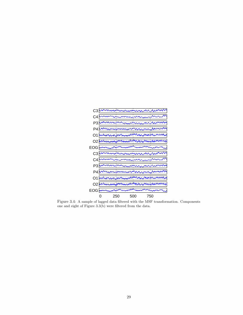
3.4 A sample of filtered lagged data. . . . . . . . . . . . . . . . . . . . . . . . . . . . . . 29

3.5 Correlations between EEG channels and the EOG channel. . . . . . . . . . . . . . . 30

3.6 Correlations between EEG channels and the EOG channel after eye blink removal. . 31

4.1 Boxplot of results on artificial data test. . . . . . . . . . . . . . . . . . . . . . . . . . 34

4.2 Performance of signal separation methods versus the length of the training signals. . 35

4.3 Boxplots of average signal correlations for three different training signal sizes. . . . . 36

vi

4.4 Boxplots of the separation performance on artificially mixed EEG data. . . . . . . . 38

4.5 Separation performance on artificially mixed EEG data versus the length of the train-

ing signals. . . . . . . . . . . . . . . . . . . . . . . . . . . . . . . . . . . . . . . . . . 39

4.6 Boxplots of separation performance on artificially mixed EEG data with time delayed

artifact propagation. . . . . . . . . . . . . . . . . . . . . . . . . . . . . . . . . . . . . 42

4.7 Separation performance versus training signal length for artificially mixed EEG data

with time delayed artifact propagation. . . . . . . . . . . . . . . . . . . . . . . . . . . 43

4.8 Average classification performance of EEG windows. . . . . . . . . . . . . . . . . . . 45

4.9 Average classification performance of EEG windows with eye blink and pulse artifacts

removed. . . . . . . . . . . . . . . . . . . . . . . . . . . . . . . . . . . . . . . . . . . . 47

4.10 Relative 60 Hz power in a set of EEG signals. . . . . . . . . . . . . . . . . . . . . . . 48

4.11 Relative 60 Hz power in the ICA components and filtered data. . . . . . . . . . . . . 48

4.12 Relative 60 Hz power in the MSF components and filtered data. . . . . . . . . . . . 48

4.13 Relative 60 Hz power in the MSF components and filtered data. . . . . . . . . . . . 49

4.14 Sine and cosine parts of the 60 Hz signal. . . . . . . . . . . . . . . . . . . . . . . . . 49

4.15 Run time for GSVD and extended Infomax versus number of samples and channels. 51

4.16 A proof of concept for a GSVD artifact filter. . . . . . . . . . . . . . . . . . . . . . . 52

vii

LIST OF TABLES

4.1 A comparison of signal separation methods on a simple artificial data set. . . . . . . 33

4.2 A comparison of signal separation methods on artificially mixed EEG data. . . . . . 38

4.3 A comparison of signal separation methods on artificially mixed EEG data with time

delayed artifact propagation. . . . . . . . . . . . . . . . . . . . . . . . . . . . . . . . 41

4.4 The means and maximum values over the classification modes. . . . . . . . . . . . . 44

4.5 Removing two artifacts: The means and maximum values over the classification modes. 46

viii

Chapter 1

Introduction

The electroencephalogram (EEG) was first measured in humans by Hans Berger in 1929. Electrical

impulses generated by nerve firings in the brain diffuse through the head and can be measured by

electrodes placed on the scalp. The EEG gives a coarse view of neural activity and has been used to

non-invasively study cognitive processes and the physiology of the brain. The analysis of EEG data

and the extraction of information from this data is a difficult problem. This problem is exacerbated

by the introduction of extraneous biologically generated and externally generated signals into the

EEG.

A current line of research involving EEG data is the development of brain-computer interfaces

(BCIs). A brain-computer interface has been defined as a “communication system that does not

depend on the brain’s normal output pathways of peripheral nerves and muscles” [56]. BCI research

aims at allowing users, typically people with motor disabilities, to communicate, via a computer,

through their EEG signals. To increase the effectiveness of BCI systems it is necessary to find

methods of increasing the signal-to-noise ratio (SNR) of the observed EEG signals. In the context

of EEG driven BCIs, the signal is endogenous brain activity measured as voltage changes at the

scalp while noise is any voltage change generated by other sources. These noise, or artifact, sources

include: line noise from the power grid, eye blinks, eye movements, heart beat, breathing, and

other muscle activity. Some artifacts, such as eye blinks, produce voltage changes of much higher

amplitude than the endogenous brain activity. In this situation the data must be discarded unless

the artifact can be removed from the data. Figure 1.1 shows an example of four seconds of EEG

data recorded at 250 samples per second from seven sites. The two spikes are the effect of eye blinks

on the recorded data. The electrical fluctuations caused by brain activity and recorded as EEG are

generally in the range of -50 to 50 microvolts, µV . Eye blinks have a higher amplitude and often

have voltages of over 100 µV .

One design of an EEG BCI system involves the classification of different mental tasks (e.g. mental

1

C3

C4

P3

P4

O1

O2

0 250 500 750 1000

EOG

Figure 1.1: A four second sample of EEG data. Electrodes are labeled according to theInternational 10-20 system shown in Figure 3.1.

multiplication or 3-D object visualization) for use in decision making [33, 3, 35]. Artifacts, even of

low amplitude, can lead to problems in this system. Consider the following scenario:

1. A BCI system is developed based on two mental tasks: mental arithmetic and imagined letter

writing.

2. The data collected to train the system contains a heart beat artifact signal.

3. The person’s heart rate is correlated with the particular mental task. For example, mental

arithmetic increases the heart rate compared to imagined letter writing. The mental task

classifier uses this difference to distinguish the two tasks.

4. While the system is in use the user wishes to make a decision corresponding to the imagined

letter writing task. For some reason the user’s heart rate is above normal and so the mental

activity is classified as mental arithmetic and an incorrect action is taken by the BCI system.

Removing signals not generated by brain activity can decrease the likelihood of this type of problem.

Even when artifacts are not correlated with tasks, they make it difficult to extract useful information

from the data.

In this thesis, novel methods of artifact removal, derived as the solutions to certain optimiza-

tion problems, are considered. The focus of this work is the use of the Maximum Signal Fraction

transformation in artifact removal. This technique is compared with the most common approaches

2

that involve the use of principal component analysis and the extended Infomax independent compo-

nent analysis algorithm [30, 31]. The mathematical development of the artifact removal techniques

considered is presented in Chapter 2. A few ideas about comparing artifact removal methods and

studying their properties are presented in Chapter 3. The experimental results are presented in

Chapter 4, and the conclusions are given in Chapter 5. Types of EEG artifacts and previous work

on their removal are considered in the next section.

1.1 Artifacts

Contamination of EEG data can occur at many points during the recording process. Most of the

artifacts considered here are biologically generated by sources external to the brain. Improving

technology can decrease externally generated artifacts, such as line noise, but biological artifact

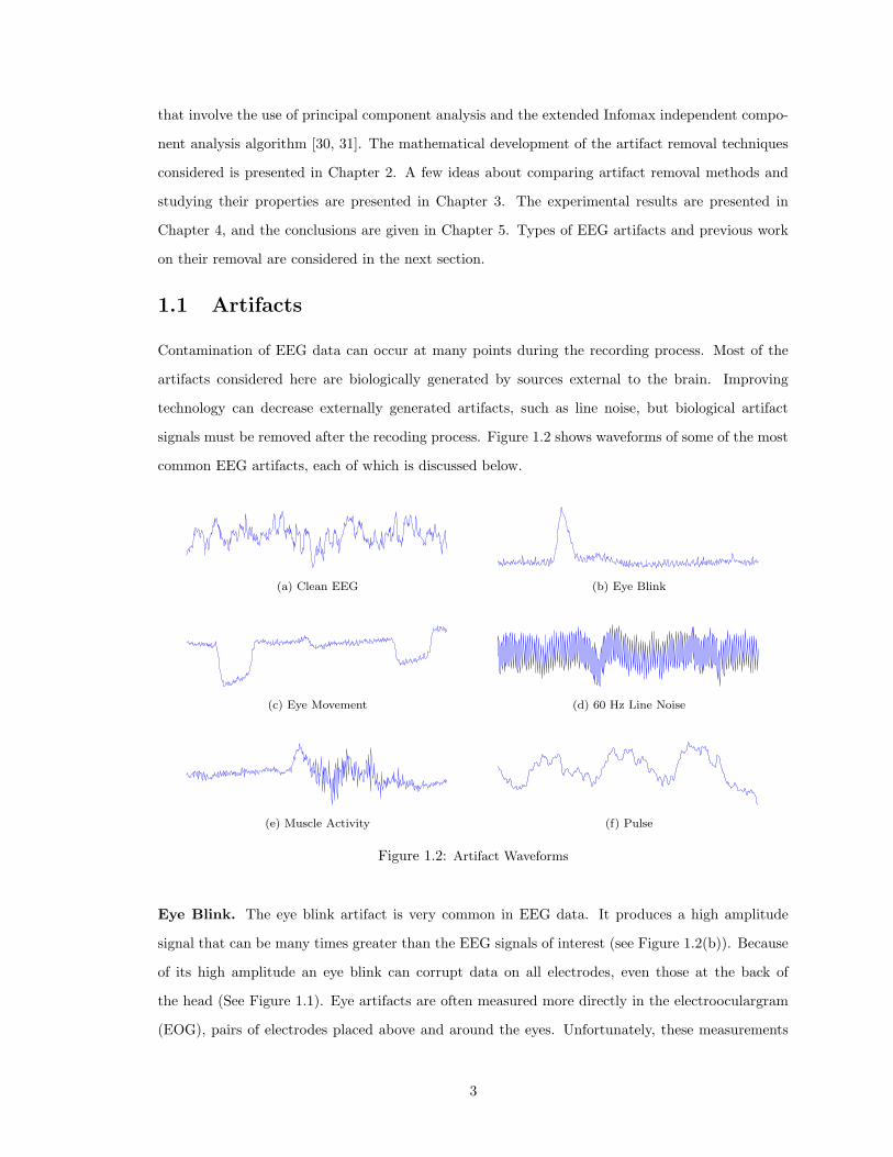
signals must be removed after the recoding process. Figure 1.2 shows waveforms of some of the most

common EEG artifacts, each of which is discussed below.

(a) Clean EEG (b) Eye Blink

(c) Eye Movement (d) 60 Hz Line Noise

(e) Muscle Activity (f) Pulse

Figure 1.2: Artifact Waveforms

Eye Blink. The eye blink artifact is very common in EEG data. It produces a high amplitude

signal that can be many times greater than the EEG signals of interest (see Figure 1.2(b)). Because

of its high amplitude an eye blink can corrupt data on all electrodes, even those at the back of

the head (See Figure 1.1). Eye artifacts are often measured more directly in the electrooculargram

(EOG), pairs of electrodes placed above and around the eyes. Unfortunately, these measurements

3

are contaminated with EEG signals of interest and so simple subtraction is not a removal option

even if an exact model of EOG diffusion across the scalp is available [31].

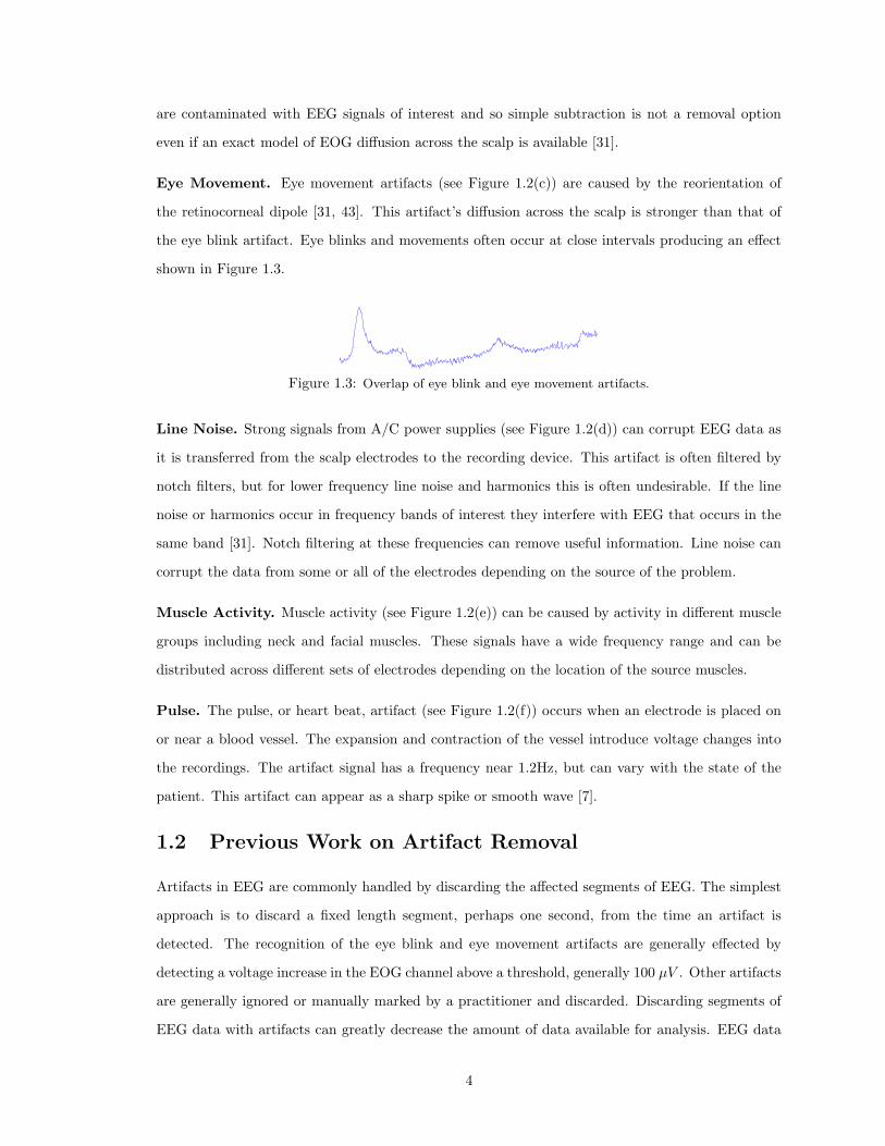
Eye Movement. Eye movement artifacts (see Figure 1.2(c)) are caused by the reorientation of

the retinocorneal dipole [31, 43]. This artifact’s diffusion across the scalp is stronger than that of

the eye blink artifact. Eye blinks and movements often occur at close intervals producing an effect

shown in Figure 1.3.

Figure 1.3: Overlap of eye blink and eye movement artifacts.

Line Noise. Strong signals from A/C power supplies (see Figure 1.2(d)) can corrupt EEG data as

it is transferred from the scalp electrodes to the recording device. This artifact is often filtered by

notch filters, but for lower frequency line noise and harmonics this is often undesirable. If the line

noise or harmonics occur in frequency bands of interest they interfere with EEG that occurs in the

same band [31]. Notch filtering at these frequencies can remove useful information. Line noise can

corrupt the data from some or all of the electrodes depending on the source of the problem.

Muscle Activity. Muscle activity (see Figure 1.2(e)) can be caused by activity in different muscle

groups including neck and facial muscles. These signals have a wide frequency range and can be

distributed across different sets of electrodes depending on the location of the source muscles.

Pulse. The pulse, or heart beat, artifact (see Figure 1.2(f)) occurs when an electrode is placed on

or near a blood vessel. The expansion and contraction of the vessel introduce voltage changes into

the recordings. The artifact signal has a frequency near 1.2Hz, but can vary with the state of the

patient. This artifact can appear as a sharp spike or smooth wave [7].

1.2 Previous Work on Artifact Removal

Artifacts in EEG are commonly handled by discarding the affected segments of EEG. The simplest

approach is to discard a fixed length segment, perhaps one second, from the time an artifact is

detected. The recognition of the eye blink and eye movement artifacts are generally effected by

detecting a voltage increase in the EOG channel above a threshold, generally 100 µV . Other artifacts

are generally ignored or manually marked by a practitioner and discarded. Discarding segments of

EEG data with artifacts can greatly decrease the amount of data available for analysis. EEG data

4

collected from children is especially problematic in this respect [16].

The first attempts at removing artifacts focused on eye blinks. Regression using the EOG channel

was attempted in the time and frequency domain [23, 21, 50, 54, 55]. These methods all rely on a

clean measure of the artifact signal to be subtracted out. Since the EOG is contaminated with EEG

signals, the regression of ocular artifacts has the undesired effect of removing EEG signals from the

observations. Regression techniques are the most common type of artifact removal in use. Recent

reviews can be found in [14, 15].

Kenemans et al. [34] give a general lagged regression model

eeg(t) = EEG(t)−T∑

g=0

βgeog(t− g),

where eeg(t) and eog(t − g) are the recorded EEG and EOG information at times t and t − g,

respectively. EEG(t) represents the uncorrupted EEG at time t, and βg measures the effect of the

EOG on eeg(t) at time t − g. Jung et al. [31] used this regression model for a baseline artifact

removal method.

More recently, multivariate statistical analysis techniques, such as principal component analysis,

have been used to separate and remove noise signals from the brain activity of interest [6, 40, 31,

32, 44, 13, 51]. This approach assumes EEG observations are generated by the linear mixing of a

number of source signals, X = SA, where Xp×n is the matrix of p, n-dimensional, observations,

Sp×m is the matrix of source signals, and Am×n is the mixing matrix. The original signals, S, and

the mixing matrix, A, are approximated by some signal separation algorithm. Recovered signals,

columns of S, that capture artifact information are removed, by setting Si = 0 where i is an artifact

column, to form S. A cleaned set of observations is then obtained by remixing the new set of signals,

X = SA. The general assumptions of this approach are:

1. the number of sources is less than or equal to the number of observations, m ≤ n;

2. the mixing is linear, X = SA; and

3. the mixing is instantaneous, X(t) = S(t)A.

Each method of signal separation applies its own assumptions as well. As discussed in Section 2.4,

independent component analysis assumes that the underlying sources are temporally independent.

Principal component analysis (see Section 2.1), on the other hand, assumes that the signals are

temporally and spatially uncorrelated.

Comparisons of artifact removal using different transformations can be found in [30, 52]. Vigon

et al. [52] compared four methods for artifact removal by artificially mixing an artifact signal from

5

one subject with a set of EEG signals from another subject. The artificial mixing matrices were

chosen to approximate mixing in the scalp. The authors found that the two independent component

analysis methods studied, Infomax and Jade [11], were significantly better than principal component

analysis and simple EOG subtraction. Performance was measured using the mean squared error

between the true artifact signal and the extracted artifact signal. Significance was measured using

an F-statistic and Tukey’s studentized range test [52]. It is not known how well artificially mixing

a signal from one subject with those of another subject approximates the actual circumstances of

artifact contamination of EEG.

The common spatial patterns (CSP) technique was used by Koles [36] to remove abnormal

components from an EEG recording. The CSP method requires the use of two data sets. The first

data set was an EEG signal contaminated by eye blink and muscle activity. The second set consisted

of data from 80 patients and was considered a true EEG signal. No quantitative evaluation was done

on the removal but it was visually observed that the artifacts were extracted into a small number

of components that would allow their removal.

Components are generally selected for removal by visual inspection, but in online filtering sys-

tems, artifact recognition is important for achieving the automatic removal of artifact signals. One

approach to recognition of noise components is based on measuring structure in the signal. The

fractal dimension and a metric based on auto-regressive (AR) coefficients have been used for this

purpose [13, 51]. Eye blinks and heart beats were found to have consistent fractal dimensions on the

data studied [51]. Jung [31] suggests that the spectral structure might be distinct for certain artifact

components (e.g., line noise) and that this would allow for automatic removal of these artifacts.

Kalman filters and extended Kalman filters have also been used for artifact detection with success

depending heavily on the artifact type [47, 45]. This approach was most successful at recognizing

one second windows containing muscle and movement artifacts.

We focus on the signal separation approach to artifact removal and present a comparison of several

methods: principal components analysis, maximum signal fraction analysis, canonical correlation

analysis, and independent component analysis. These signal separation techniques are introduced

in the next chapter. Comparison with other artifact removal approaches is left for future work.

6

Chapter 2

Mathematical Background

The mathematics needed for the artifact removal methods in this study are presented here. EEG

data will be represented by the matrix Xp×n where p is the number of samples and n is the number

of electrodes. Each column of X contains the data recorded from a single electrode and each row

is the data from all electrodes at one point in time. X (i) will represent the ith row, henceforth,

a data point, and Xi will be the ith column, a signal or channel. Each of the transformations

described below are applied to a small sample of EEG, shown in Figure 1.1, for illustrative purposes.

The columns of the mixing matrix A can be viewed as topographic maps on the scalp showing

the influence of each recovered source signal on the observations at each electrode. The EEGLAB

Matlab toolbox[17] was used to generate these scalp plots.

2.1 Principal Component Analysis

Principal component analysis (PCA) can be developed from many different points of view, but it

will be most useful in the context of artifact removal to view PCA as an optimization problem.

PCA finds a linear transformation of a data set that maximizes the variance of the transformed

variables subject to orthogonality constraints on the transformation and transformed variables. The

transformation is found by solving the following optimization problem:

maxα‖Xα‖2 = max

αα′X ′Xα subject to α′α = 1. (2.1)

The solution, α, gives the linear combination of the observations with maximum variance. The

complete set of solutions can be defined recursively by

maxα

α⊥α1,...,αk

α′X ′Xα subject to α′α = α′1α1 = . . . = α′kαk = 1 for k < rank(X).

7

The solutions to this problem are the eigenvectors of X ′X which can be found by solving the

eigenvalue problem

X ′Xα = λα

where α is an eigenvector and λ is the corresponding eigenvalue [24]. Since the optimization problem

in Equation (2.1) is convex, it has a single optimum. It is well known that solving Equation (2.1)

for all eigenvectors is equivalent to computing the singular value decomposition (SVD) of X

Xp×n

= Up×p

Σp×n

V ′n×n

,

where the columns of V , the right singular vectors, are the eigenvectors of X ′X [24]. The transfor-

mation X = XV produces a new set of orthogonal variables ordered by decreasing variance. Figure

2.1 shows the SVD defined transformation on a four second sample of EEG data. The columns of X

are shown and the first component has the most variance. Figure 2.2 shows the extracted signals, X,

and the influence of these signals on the observations at each electrode. These weightings are given

by the approximated mixing matrix V −1 = V ′. The effect of the spatial orthogonality constraint

can be seen in the topographic maps for Signal 6. Signal 6 has an effect on the observations at the

P3, C4, and EOG electrodes, but not at its other neighboring electrodes. The spatial distribution

of this extracted signal clearly indicates that it is not a true source signal in the EEG.

C3

C4

P3

P4

O1

O2

0 250 500 750 1000

EOG

(a) EEG

1

2

3

4

5

6

0 250 500 750 1000

7

(b) SVD

Figure 2.1: The SVD transformation of a small EEG sample.

8

1

2

3

4

5

6

0 250 500 750 1000

7

Figure 2.2: The topographic scalp maps of the SVD decomposition.

9

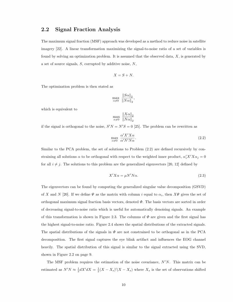
2.2 Signal Fraction Analysis

The maximum signal fraction (MSF) approach was developed as a method to reduce noise in satellite

imagery [22]. A linear transformation maximizing the signal-to-noise ratio of a set of variables is

found by solving an optimization problem. It is assumed that the observed data, X, is generated by

a set of source signals, S, corrupted by additive noise, N ,

X = S +N.

The optimization problem is then stated as

maxα6=0

‖Sα‖2‖Nα‖2

,

which is equivalent to

maxα6=0

‖Xα‖2‖Nα‖2

if the signal is orthogonal to the noise, S ′N = N ′S = 0 [25]. The problem can be rewritten as

maxα6=0

α′X ′Xα

α′N ′Nα. (2.2)

Similar to the PCA problem, the set of solutions to Problem (2.2) are defined recursively by con-

straining all solutions α to be orthogonal with respect to the weighted inner product, α′iX′Xαj = 0

for all i 6= j. The solutions to this problem are the generalized eigenvectors [20, 12] defined by

X ′Xα = µN ′Nα. (2.3)

The eigenvectors can be found by computing the generalized singular value decomposition (GSVD)

of X and N [20]. If we define Ψ as the matrix with column i equal to αi, then XΨ gives the set of

orthogonal maximum signal fraction basis vectors, denoted Φ. The basis vectors are sorted in order

of decreasing signal-to-noise ratio which is useful for automatically denoising signals. An example

of this transformation is shown in Figure 2.3. The columns of Φ are given and the first signal has

the highest signal-to-noise ratio. Figure 2.4 shows the spatial distributions of the extracted signals.

The spatial distributions of the signals in Φ are not constrained to be orthogonal as in the PCA

decomposition. The first signal captures the eye blink artifact and influences the EOG channel

heavily. The spatial distribution of this signal is similar to the signal extracted using the SVD,

shown in Figure 2.2 on page 9.

The MSF problem requires the estimation of the noise covariance, N ′N . This matrix can be

estimated as N ′N ≈ 12dX

′dX = 12 (X − Xs)

′(X − Xs) where Xs is the set of observations shifted

10

C3

C4

P3

P4

O1

O2

0 250 500 750 1000

EOG

(a) EEG

1

2

3

4

5

6

0 250 500 750 1000

7

(b) MSF

Figure 2.3: The MSF transformation of a small EEG sample.

forward by one time step [22]. This method of estimating the noise requires certain assumptions

which can be seen by expanding dX ′dX:

dX ′dX = (X −Xs)′(X −Xs)

= (S +N − Ss −Ns)′(S +N − Ss −Ns)

= ((S − Ss) + (N −Ns))′((S − Ss) + (N −Ns))

= (S − Ss)′(S − Ss) + (N −Ns)′(S − Ss)

+(S − Ss)′(N −Ns) + (N −Ns)′(N −Ns).

Under the assumption that S ′N = N ′S = 0 the middle terms become zero. Expanding the last term

gives

dX ′dX ≈ (S − Ss)′(S − Ss) + (N −Ns)′(N −Ns)

≈ (S − Ss)′(S − Ss) +N ′N −Ns′N −N ′Ns +Ns′Ns.

Assuming that the noise is temporally uncorrelated, Ns′N = N ′Ns = 0. Since N ′N ≈ Ns

′Ns,

1

2dX ′dX ≈ N ′N + (S − Ss)′(S − Ss).

If the signal is smooth then S−Ss will be near zero and the last term will drop out and give a good

estimate of the noise. It has been observed that this technique can produce good results even when

11

1

2

3

4

5

6

0 250 500 750 1000

7

Figure 2.4: The topographic scalp maps of the MSF decomposition.

12

the assumptions are met only approximately [26].

As noted above the solution to the maximum signal fraction problem can be found by the

generalized singular value decomposition. By considering the covariance matrices of two classes of

data rather than the signal and noise covariance, a more general procedure can be developed. Let

A and B be the two classes of data. The GSVD decomposition can be defined as

Ap×n

= Up×p

Cp×n

X ′n×n

Bq×n

= Vq×q

Sq×n

X ′n×n

where C2 + S2 = I [20]. Since the GSVD yields a joint diagonalization of A′A and B′B as

A′A = XC2X ′

B′B = XS2X ′,

a useful observation can be made about the projections UC and V S. The variance of A captured

in UC decreases from the left column to the right column while the variance of B captured in V S

decreases from right to left. The coordinate that captures the most variance of A captures the least

variance of B, and vice versa, because of the constraint that C2+S2 = I. When A = X and B = N ,

we can say that the first columns of UC capture most of the signal, while the last columns of V S

capture most of the noise. This approach has been called common spatial patterns (CSP) [18, 46,

42, 41] and appears to have been first used in the context of EEG analysis by Koles [36, 48, 37]. See

Appendix A for the relation of CSP, as presented in [36], and the GSVD.

Another view of the MSF, important to artifact removal, is developed by noting that the MSF

transform is, under certain assumptions, equivalent to second order blind source separation (BSS)

[25, 26]. Assuming that dS ′dS = I where dS = (S −Ss) and that S′S = λs 6= σI, with λs diagonal,

then solving Problem (2.3) gives the solutions, S and A, to the BSS problem

Xp×n

= Sp×n

An×n

.

Letting A = Ψ †, where Ψ is the matrix of solutions to Problem (2.3) and Ψ † is its pseudo-inverse,

gives the desired solution [25].

The mixing matrix A can be found by solving for the components of its SVD, A = UAΣAV′A.

The derivation here follows [25] and [26]. Consider dX ′dX under the model assumption X = SA,

and note that

dX ′dX = A′dS′dSA = A′A = VAΣ2AV

′A

13

with the assumption that dS ′dS = I. Applying the whitening transformation, VAΣ−1A , to X yields

X = XVAΣ−1A = SAVAΣ

−1A = SUAΣAV

′AVAΣ

−1A = SUA.

Using the assumption that S ′S = λs, UA is found by

X ′X = U ′AS′SUA = U ′AλsUA.

Since λs 6= σI, it does not commute with UA, and the source signals, S, can be found by

S = XVAΣ−1A U ′A = SA−1.

The connection to MSF can be made by solving Problem (2.2) by a double whitening process,

similar to the computation of A above. First, compute the SVD decomposition

dX = U1Σ1V′1

and note that by applying the whitening transformation, V1Σ−11 , to X and dX, the Problem (2.2)

can be transformed into

maxα 6=0

α′Σ−11 V ′1X

′XV1Σ−11 α

α′Σ−11 V ′1dX

′dXV1Σ−11 α

= maxα 6=0

α′X ′Xα

α′α.

As discussed in Section 2.1, the solutions to the above problem are found by computing the SVD of

X:

X = U2Σ2V′2 .

The set of solutions in V2 must be transformed back into the original space. The solutions to the

original MSF problem are

Ψ ≡ V1Σ−11 V2.

Finally, note that V2 = U ′A and V1Σ−11 = VAΣ

−1A which gives

Ψ = VAΣ−1A U ′A = A†

such that XΨ = SAA† = S.

2.3 Canonical Correlation Analysis

Canonical correlation analysis (CCA) is a method of extracting similarity between two data sets. In

this section it is assumed that the set of EEG observations has been partitioned into two sets, X

and Y , perhaps left hemisphere electrodes and right hemisphere electrodes. CCA finds two linear

14

transformations, one for X and the other for Y , that maximize the correlation of X and Y in the

new coordinates.

Given two sets of observations Xp×n1and Yp×n2

, consider the linear projections a = Xψa and

b = Y ψb. The correlation between a and b is given by

ρ(a, b) =E{ab}

√

E{a2}E{b2}=

ψTaXTY ψb√

ψTaXTXψa

√ψTb Y

TY ψb.

The canonical correlations are given by maximizing ρ(a, b) over all non-zero linear projections

maxψa,ψb 6=0

ψTaXTY ψb√

ψTaXTXψa

√ψTb Y

TY ψb. (2.4)

The solutions, Ψa and Ψb, can be found using the QR decompositions of X and Y [57]. Let

X = QxRx and Y = QyRy with Qx and Qy orthogonal and Rx and Ry upper triangular. Take the

SVD of Q′xQy

Q′xQy = ECF ′

and the canonical correlations are given by the diagonal elements of C. The transformations Ψa and

Ψb are found by taking Ψa = R−1x E and Ψb = R−1

y F . The transformed data can be computed by

taking X = XΨa = QxRxΨa = QxE and Y = Y Ψb = QyRyΨb = QyF . The columns of, X and Y ,

are ordered by decreasing cross-correlation.

CCA can be used for signal separation by taking as X and Y a data matrix X and a shifted

version of itself, Xs, respectively [10, 9]. In this context the CCA optimization criterion results

in projections that maximize the autocorrelation of the projected signals. Under the assumption

that the signals are orthogonal, S ′S = 0, the autocorrelation of a mixture of the signals is bounded

by the maximum autocorrelation of the individual signals [10]. A projection that maximizes the

autocorrelation of the data in new coordinates will separate the signals because of this constraint.

The CCA transformation was applied to the sample EEG used in the previous examples. Shown in

Figure 2.5 is X, which will be used for all of the experiments (rather than Y ). Figure 2.6 shows the

topographic maps associated with each extracted signal. The spatial distributions of these signals

are very similar to those extracted by the MSF method.

In this context there is a strong similarity between the optimization criteria for CCA and MSF.

Given enough data and letting Y = Xs, it can be assumed that X ′X = Xs′Xs and that ψa = ψb.

Now Equation (2.4) is

maxψa 6=0

ψTaXTXT

s ψa

ψTaXTXψa

. (2.5)

The solution is a projection that maximizes the 1-lag autocorrelation of the projected variable. Now

15

C3

C4

P3

P4

O1

O2

0 250 500 750 1000

EOG

(a) EEG

2

3

4

5

6

0 250 500 750

7

1

(b) CCA

Figure 2.5: The CCA transformation of a small EEG sample.

consider the MSF optimization problem

maxψ 6=0

ψTXTXψ

ψTNTNψ. (2.6)

Maximizing the inverse of Equation (2.6) gives the same solutions in opposite order. Letting N TN =

12 (X −Xs)

T (X −Xs) gives

maxψ 6=0

ψTNTNψ

ψTXTXψ= max

ψ 6=0

12ψ

T (XTX +XTXs +XTs X +XT

s Xs)ψ

ψTXTXψ

= maxψ 6=0

ψT (XTX + 12X

TXs +12X

Ts X)ψ

ψTXTXψ

= 1 +maxψ 6=0

ψT ( 12X

TXs +12X

Ts X)ψ

ψTXTXψ

which is clearly related to the CCA optimization problem in (2.4). The similarity in the optimization

criteria and the fact that both methods perform second-order blind signal separation under similar

assumptions gives strong evidence for believing that they will perform similarly in the artifact

removal task.

2.4 Independent Component Analysis

Whereas PCA, MSF, and CCA extract uncorrelated signals that optimize some criterion, indepen-

dent component analysis (ICA) is defined as extracting independent signals from a data set. The

16

1

2

3

4

5

6

0 250 500 750 1000

7

Figure 2.6: The topographic scalp maps of the CCA decomposition.

17

problem is formulated by assuming that a set of observations, X, is generated by a linear mixing,

SA, of a set of independent signals, S, by a mixing matrix A. An unmixing matrix, W , is found

by optimizing some measure of the independence of the unmixed signals, XW . Since orthogonal

transformations of Gaussian variables do not change their distributions, all but one of the sources, S,

must be non-Gaussian in order for A to be well determined [28]. An example of the signals extracted

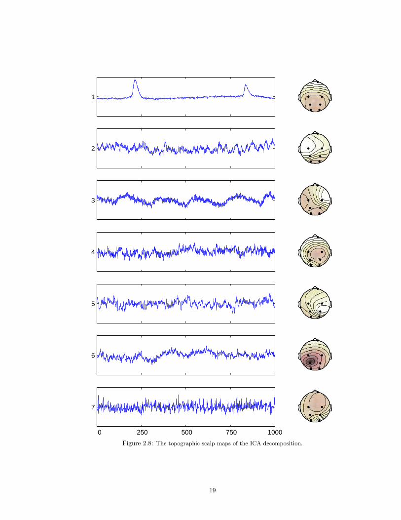
by the extended Infomax method, described below, is given in Figure 2.7. The spatial distributions

of the signals, taken from W−1, are shown in Figure 2.8. Similar to the MSF method, ICA only

requires that the matrix W be invertible.

C3

C4

P3

P4

O1

O2

0 250 500 750 1000

EOG

(a) EEG

2

3

4

5

6

0 250 500 750 1000

7

1

(b) Infomax

Figure 2.7: The ICA separation of a four second EEG sample.

The difficulty with ICA is that measuring independence is computationally intractable. This

leads to the need for approximate measures of independence of which there are many. One approach,

used in the Infomax algorithm, is to minimize the mutual information between the recovered signals,

XW . This can be approximated by maximizing the mutual information between the set of inputs,

X and the outputs, XW [5]. The solution derived uses a gradient-based search through the space of

unmixing matrices, W . The gradient descent search is an iterative process and makes the Infomax

more time consuming to compute than any of the previously discussed methods.

The description here follows the development in [39]. Given a set of independent source signals,

18

1

2

3

4

5

6

0 250 500 750 1000

7

Figure 2.8: The topographic scalp maps of the ICA decomposition.

19

S, the probability density function can be written as

p(S) =

N∏

j=1

pj(Sj).

The observations are generated byX = SA and the mutual information between the observed signals

is given by

I(X) =

∫

p(X) logp(X)

∏Ni=1 pi(Xi)

dX

and measures the divergence of p(X) from the factored distribution,∏Ni=1 pi(Xi), that assumes the

observation variables are independent. The mutual information, I(X) equals zero when the signals

in X are independent. Given an unmixing matrix, W , a new set of signals, X is obtained through

X = XW = SAW . The goal of ICA is to find a matrix, W , so that the new signals have I(X) = 0.

To find W , a maximum likelihood learning rule is derived by taking

p(X) = |detW | p(X) = |detW |N∏

i=1

pi(Xi).

The log likelihood of p(X) is given by

L(X,W ) = log |detW |+N∑

i=1

log pi(Xi).

Bell and Sejnowski derived the maximum likelihood learning rule in the original Infomax ICA paper

[5],

∆W ∝[

(W ′)−1 − φ(X)X ′]

with

φ(X) = −∂p(X)

∂X

p(X).

This learning rule was subsequently improved in [2] by using the natural gradient,

∆W ∝ ∂L(X,W )

∂WW ′W =

[

I − φ(X)X ′]

W.

The natural gradient gives much faster convergence and does not require the computation of W−1

at every iteration.

Since pi(Xi) is unknown, φ(X) is approximated by a non-linear function, g(X). The choice of

function is important to the success of the separation [39]. A common choice is to let g(X) = 2 tanh X

which allows for the separation of super-Gaussian sources [27]. A method for separating both super-

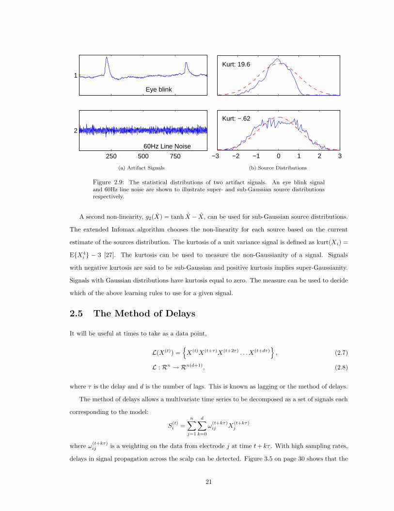
and sub-Gaussian sources was derived in [39]. Examples of super- and sub-Gaussian sources are

given in Figure 2.9.

20

1

250 500 750

2

Eye blink

60Hz Line Noise

(a) Artifact Signals

−3 −2 −1 0 1 2 3

Kurt: 19.6

Kurt: −.62

(b) Source Distributions

Figure 2.9: The statistical distributions of two artifact signals. An eye blink signaland 60Hz line noise are shown to illustrate super- and sub-Gaussian source distributionsrespectively.

A second non-linearity, g2(X) = tanh X − X, can be used for sub-Gaussian source distributions.

The extended Infomax algorithm chooses the non-linearity for each source based on the current

estimate of the sources distribution. The kurtosis of a unit variance signal is defined as kurt(Xi) =

E{X4i } − 3 [27]. The kurtosis can be used to measure the non-Gaussianity of a signal. Signals

with negative kurtosis are said to be sub-Gaussian and positive kurtosis implies super-Gaussianity.

Signals with Gaussian distributions have kurtosis equal to zero. The measure can be used to decide

which of the above learning rules to use for a given signal.

2.5 The Method of Delays

It will be useful at times to take as a data point,

L(X(t)) ={

X(t)X(t+τ)X(t+2τ) . . . X(t+dτ)}

, (2.7)

L : Rn → Rn(d+1), (2.8)

where τ is the delay and d is the number of lags. This is known as lagging or the method of delays.

The method of delays allows a multivariate time series to be decomposed as a set of signals each

corresponding to the model:

S(t)i =

n∑

j=1

d∑

k=0

ω(t+kτ)ij X

(t+kτ)j

where ω(t+kτ)ij is a weighting on the data from electrode j at time t+ kτ . With high sampling rates,

delays in signal propagation across the scalp can be detected. Figure 3.5 on page 30 shows that the

21

maximum correlation between the occipital electrodes, O1 and O2, and the EOG channel occurs not

instantaneously, at shift 0, but in the negative 2 to 4 shift range representing 8 to 16 micro-seconds.

Thus, the eye blink signal takes a small number of time steps to reach the back of the head. Lagging

the observations is a way of taking this effect into account when performing analysis of EEG data.

Taken’s theorem [49] also provides an argument for this embedding of the data. Assuming that

the EEG is generated by a dynamical system, a reconstruction of the dynamics of this system can

be obtained by including enough lags. If the trajectory lies on a D dimensional set, then d > 2D is a

sufficient embedding dimension (number of lags) to reconstruct the system [49, 1]. This embedding

may provide information that allows for better artifact removal.

2.6 Classification

BCI systems require the classification of different EEG patterns for the transfer of information from

brain to computer. The analysis of classification methods is not important to this work so a simple

classifier will be used. The Bayes optimal classifier is based on the likelihood ratio of class probability

distributions [19]. For Gaussian distributions the optimal classifier is defined by the discriminant

functions

gi(x) = −1

2(x− µi)′Σ−1

i (x− µi)−1

2log |Σi|+ logP (ωi),

where P (ωi) is the prior probability for class i, µi is the class mean, and Σi is the class covariance,

which must be invertible. A point x is assigned to class i if gi(x) > gj(x) ∀ j 6= i. This is known as

the quadratic discriminant classifier because the discriminant function is quadratic in x.

The raw EEG signals do not contain enough discriminatory information to be correctly classified

by mental task with the quadratic discriminant classifier [35]. A representation that has successfully

been used in classifying mental tasks involves creating overlapping windows of data and using some

or all of the right singular vectors of each window as a point in classification space [35, 4]. EEG

signals recorded at six locations were partitioned into windows of 1/2 second of data, sampled at

250Hz, that overlap by 1/4 second. It was also observed in [35] that lagging the data can increase

classification accuracy. The algorithm below represents the number of lags by d. The representation

is generated by:

For all windows, X125×6(d+1)

Take the SVD of X125×6(d+1) = UΣ V ′ where V ∈ R6(d+1)×6(d+1)

Let Y = [V ′k1V′k2. . . V ′kn ], where Vki is a column of V

22

End

The discriminant function is determined by the set of points, Y , in R6n(d+1) and their labels.

Recent results show this to be an effective classification technique for spontaneous EEG data [35].

In Section 4.4 each column of V is used independently to produce 6(d+ 1) classification results.

23

Chapter 3

Methods

3.1 EEG Data

EEG is most commonly recorded according to the international 10-20 electrode placement system

shown in Figure 3.1 [29]. The 10-20 system was developed to standardize the collection of EEG and

facilitate the comparison of studies performed at different laboratories. When only a few channels of

EEG are collected the electrodes are placed at a subset of the sites. For example, Figure 1.1 on page

2 shows data collected from only six electrodes and an EOG channel. The EOG channel generally

consists of two electrodes referenced to each other. The recorded signal is obtained by subtracting

a signal measured below the eye from one measured above the eye.

Figure 3.1: The International 10-20 electrode placement system.

The data used in the following chapter and shown in the examples of the previous chapter was

recorded in 1988 by Zachary Keirn for his Masters Thesis in Electrical Engineering, at Purdue

24

University [33]. The recordings were referenced with electrically linked mastoid recordings at A1

and A2 and recorded at six sites: C3, C4, P3, P4, O1, and O2. A bank of Grass 7P511 amplifiers

with bandpass settings of 0.1 to 100 Hz was used to record the data. The data was stored at 250

samples per second and digitized with twelve bits of accuracy. Sets of ten second trials were recorded

for each of five mental tasks: resting task, imagined letter writing, mental multiplication, visualized

counting, and geometric object rotation. The tasks were chosen in an attempt to illicit different

spatial patterns which could be used for classification. For the experiments with artificially mixed

EEGs described in Sections 4.2 and 4.3, data from subjects one and two was used. In Section 4.4

data from subject one for the imagined letter writing and visualized counting tasks was used.

For the imagined letter writing task, the subject was asked to compose a letter without vocalizing

the composition. In subsequent trials the subject was asked to continue the letter from a previous

stopping point. In the visual counting task each subject was asked to visualize numbers being

written on a blackboard, with each number being erased before the following number was written.

The subjects were asked not to vocalize the numbers and to start each trial where the previous left

off.

3.2 Using Linear Transformations to Remove Artifacts

The use of linear transformations for artifact removal was briefly described in Section 1.2. Here the

mathematical techniques described in the previous chapter are discussed in the context of artifact

removal.

The principal component analysis technique, or equivalently, the singular value decomposition

(SVD), is limited in its signal separation capabilities by the simultaneous constraints of temporal and

spatial orthogonality. For an artifact signal to be separated by the SVD, it must have high variance

or it will be mixed with other components. For some large amplitude eye blinks this assumption

may be met, but the SVD will generally not be successful at removing other lower amplitude artifact

signals.

The maximum signal fraction (MSF) transform enforces temporal decorrelation of the extracted

components but only constrains the spatial patterns to forming an invertible matrix. The optimiza-

tion criteria used to derive this technique allows the sorting of the transformed signals in order of

decreasing signal-to-noise ratio. The ordering can be used to help automatically denoise signals

since low signal-to-noise ratio components can be filtered out. Eye blink artifacts tend to have high

signal-to-noise ratios and are generally the first or second component.

The canonical correlation analysis (CCA) approach to signal separation requires that the signals

25

to be separated have different 1-lag autocorrelation structures. This assumption should be met

for most artifacts since they have quite different time courses, see Figure 1.2. It should be noted

that in preliminary studies the CCA approach produced signals very similar to those extracted by

the MSF transform. The signals were also sorted in the same order and the signal-to-noise ratios

were similar to the canonical correlations. Some of this may be explained by the similarity of the

optimization criteria mentioned in the previous section, but there is also a relationship between the

autocorrelation and signal-to-noise ratio pointed out in [8].

The Infomax ICA algorithm assumes that the underlying sources of interest are temporally in-

dependent. When studying spontaneous EEG activity, this assumption should be safe since there

are no specific external stimuli causing the generation of specific time locked EEG patterns. The ex-

tended Infomax algorithm which can extract sub-Gaussian sources, such as 60Hz line noise, requires

the computation of the kurtosis of the extracted signals. This computation requires at least 2000

data samples for accurate computation [17]. This requirement is not always met in the experiments,

but does not seem to have an extreme effect on the performance.

Given a set of EEG observations Xp×n and a transformation matrix Wn×n computed using one

of the methods in Chapter 2, the estimated source signals are obtained by S = XW . Artifact

components are visually selected for removal and are set to zero by taking S(i) = 0. This operation

can be represented as a right multiplication by a matrix Z where Zii = 1 if a signal is not an artifact,

Zii = 0 if signal i is an artifact, and Zij = 0 for all i 6= j. The modified version of S is given by

S = SZ. The filtered data can be computed by inverting the unmixing transformation,

X = SW−1 = SZW−1.

Substituting XW for S gives

X = SZW−1 = XWZW−1 = XP,

where the artifact filter, P , is defined by P = WZW−1. Applying this transformation to X, or a

new data set, by X = XP , has the same effects as setting columns of S to zeros and inverting the

transformation by SW−1 (see Section 1.2). This algorithm for the construction of artifact filters will

be used in Chapter 4 where the different methods are compared. For illustrative purposes, consider

the example MSF transform in Figure 2.3. The first signal is marked as an eye blink artifact and

the first column of Ψ is set to zero. Then the artifact filter, P , is defined by P = ΨZΨ−1. The

filtered data, XP , is shown in Figure 3.2. Visual inspection suggests that much of the eye blinks at

samples 225 and 800 has been removed from the data.

26

C3

C4

P3

P4

O1

O2

0 250 500 750 1000

EOG

(a) EEG

C3

C4

P3

P4

O1

O2

0 250 500 750 1000

EOG

(b) MSF Filtered Data

Figure 3.2: An example of data filtered using the MSF method.

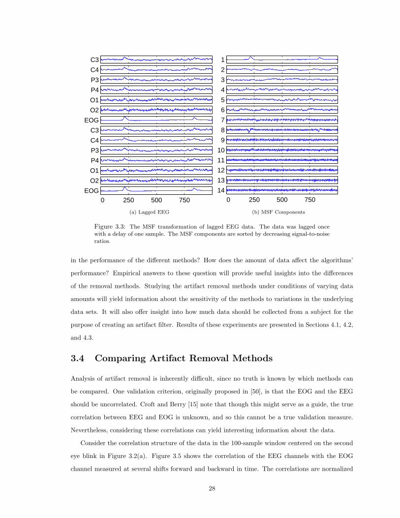
As discussed in Section 2.5, it may be beneficial to combine the method of delays with the artifact

removal approach described above. An example is given to illustrate the process and the problems

involved. Figure 3.3 shows the data from Figure 1.1 lagged once with a delay of one and the MSF

components of this data set. Components one and eight were removed as described in the previous

paragraph, and the filtered set of data in Figure 3.4 was obtained. The two sets of filtered channels

are not the same, so the problem is to decide which set of filtered data channels to use in subsequent

analysis. In all of the experiments involving filtered lagged data, the first set of filtered signals is

chosen. The problem of which set to choose, or whether to possibly average the sets, is left for

future research. Section 3.4 gives example that illustrates why lagging EEG data may be beneficial

for artifact removal.

3.3 Characteristics of the Signal Separation Methods

Before studying the artifact removal methods on real EEG data, it will be useful to study certain

characteristics of the signal separation methods used for artifact removal on simple data. With

simple data, the true solution is known so there is a baseline for comparing the techniques. Analysis

will be performed in three different scenarios: mixing of artificial signals, artificial mixing of EEG

data, and artificial mixing of EEG with propagation delay of the artifact signal. How well do the

separated signals correlate with the original signals? Are there statistically significant differences

27

C3

C4

P3

P4

O1

O2

EOG

C3

C4

P3

P4

O1

O2

0 250 500 750EOG

(a) Lagged EEG

1

2

3

4

5

6

7

8

9

10

11

12

13

0 250 500 75014

(b) MSF Components

Figure 3.3: The MSF transformation of lagged EEG data. The data was lagged oncewith a delay of one sample. The MSF components are sorted by decreasing signal-to-noiseratios.

in the performance of the different methods? How does the amount of data affect the algorithms’

performance? Empirical answers to these question will provide useful insights into the differences

of the removal methods. Studying the artifact removal methods under conditions of varying data

amounts will yield information about the sensitivity of the methods to variations in the underlying

data sets. It will also offer insight into how much data should be collected from a subject for the

purpose of creating an artifact filter. Results of these experiments are presented in Sections 4.1, 4.2,

and 4.3.

3.4 Comparing Artifact Removal Methods

Analysis of artifact removal is inherently difficult, since no truth is known by which methods can

be compared. One validation criterion, originally proposed in [50], is that the EOG and the EEG

should be uncorrelated. Croft and Berry [15] note that though this might serve as a guide, the true

correlation between EEG and EOG is unknown, and so this cannot be a true validation measure.

Nevertheless, considering these correlations can yield interesting information about the data.

Consider the correlation structure of the data in the 100-sample window centered on the second

eye blink in Figure 3.2(a). Figure 3.5 shows the correlation of the EEG channels with the EOG

channel measured at several shifts forward and backward in time. The correlations are normalized

28

C3

C4

P3

P4

O1

O2

EOG

C3

C4

P3

P4

O1

O2

0 250 500 750EOG

Figure 3.4: A sample of lagged data filtered with the MSF transformation. Componentsone and eight of Figure 3.3(b) were filtered from the data.

29

so that the autocorrelation of the EOG channel is one at shift zero. Channels C4 and P4 are

maximized at shift zero and have the highest correlations with the EOG channel. The maximum

correlations in the other channels are lower and decrease with distance from the EOG electrodes.

Figure 3.6 shows the correlation structure of the same eye blink for the MSF filtered data in Figure

3.2. In most of the channels the correlation with the EOG channel has been greatly decreased. This

might signify successful artifact removal, but, as mentioned above, it is difficult to make this claim

with certainty because of the contamination of the EOG channel with EEG data.

−10 −5 0 5 100

0.2

0.4

0.6

0.8

1Cross Correlation with the EOG Channel

Cor

rela

tion

Shift

C3C4P3P4O1O2

Figure 3.5: The structure of the correlations between EEG channels and the EOG chan-nel provides useful information about the eye blink artifact. The cross correlations werecomputed across -10 to 10 sample shifts of the EEG channels with respect to the EOGchannel. A maximum correlation at a negative shift means the signal is preceded by theEOG channel.

As a brief aside, note that Figure 3.5 shows the maximum correlation occurs at up to a four sample

negative shift from the EOG channel. This implies that the EOG signal is delayed as it propagates

through the scalp, up to 16 micro-seconds, and brings into question the third assumption, that

the signals are instantaneously mixed, as discussed in Section 1.2. This observation suggests that

combining the maximum signal fraction method with lagged data might improve artifact removal

performance. Also, note the cyclic The cyclic structure of the correlations in Figure 3.6 are the

result of 60 Hz line noise not seen until the eye blink was removed.

A novel approach to comparing artifact removal methods is developed using the mental task

classification problem: artifact methods are compared in an indirect fashion by their effect on the

classification of different tasks. Removing artifacts reveals the true underlying mental activity which

30

−10 −5 0 5 100

0.2

0.4

0.6

0.8

1Cross Correlation with the EOG Channel

Shift

Cor

rela

tion

C3C4P3P4O1O2

Figure 3.6: Correlation structure of sample in Figure 1.1 after the eye blink has beenremoved using the MSF transformation. The maximum correlations have decreased and aperiodic structure, caused by 60Hz line noise is revealed.

is assumed to be more strongly correlated with a given mental task than the artifact corrupted

data. Removing these extraneous noise signals should improve the classification performance on

windows of data containing artifacts. Artifact removal should not negatively affect classification

of those data windows that do no contain artifact signals. When an algorithm negatively impacts

classification accuracy, comparison becomes more difficult because it cannot be determined whether

the classification algorithm was relying on artifacts for discrimination or whether the artifact remover

has removed discriminatory information from the underlying brain data. Nevertheless, changes in

classification rates can be used to discern information about the different artifact removers and about

the interplay between artifact removal and classification of mental task data in general. Results of

this experiment are presented in Section 4.4.

31

Chapter 4

Results

The present chapter explores the different artifact removal methods described in the previous two

chapters. The hypothesis is that the maximum signal fraction (MSF) transform can perform as

well as the extended Infomax (ICA) approach in this domain. The experiments that follow provide

evidence that the MSF method can be used to successfully remove artifacts from EEG and that it

may have benefits over the ICA method. Both the ICA and MSF approaches are shown to remove

artifacts from EEG data without negatively impacting classification of mental task data. It is also

observed that combining lagging with the MSF transform is more successful at removing line noise

than the ICA algorithm.

The first three sections present experiments involving artificially generated data sets. Separation

of artificially mixed signals is considered under varying amount of data and performance is measured

using correlation with the known solution. In the fourth section, an analysis is presented on the

mental task classification problem. Section 4.5 considers removal of the line noise artifact using

the MSF transform and ICA. The time for computing the MSF and ICA transforms is explored in

Section 4.6. The last section considers other approaches to using the GSVD for artifact removal.

4.1 A Test on Simple Signals

An initial comparison of the signal separation methods used for artifact removal was made on sets of

artificial signals. The signals were generated by mixing a sine wave, a cosine wave, and a Gaussian

noise signal, each of 900 samples. The frequencies of the sine and cosine wave was varied from

0.4 Hz to 5 Hz, assuming a 250 Hz sampling frequency, over 200 trials. The mixing matrix was

also varied with each trial and the Gaussian noise signal was randomly generated for each of the

trials. The signal separation methods were applied to each trial and the correlations of the extracted

signals with the true signals were recorded. The means and standard deviations of the correlations

32

are shown in Table 4.1. The table shows that the SVD performs about 10% worse than the other

methods. The MSF, CCA, and ICA methods perform similarly, but note that the MSF and CCA

methods have lower variance and better performance separating the Gaussian noise signal than does

ICA.

Sin Cos Gaussian Noise AveSVD 0.9145 (0.0885) 0.8728 (0.1037) 0.8661 (0.1139) 0.8845 (0.0765)MSF 0.9948 (0.0243) 0.9913 (0.0394) 0.9989 (0.0011) 0.9950 (0.0186)CCA 0.9941 (0.0309) 0.9925 (0.0305) 0.9989 (0.0011) 0.9952 (0.0168)ICA 0.9947 (0.0239) 0.9931 (0.0288) 0.9909 (0.0418) 0.9929 (0.0236)

Table 4.1: A comparison of signal separation methods on a simple artificial data set. Themeans are given with the standard deviations in parentheses. The correlation betweeneach extracted signal and the original signal was measured.

The box plot in Figure 4.1 shows the complete set of results for the 200 trials. The median is

the centerline of the box, and the angled lines show the confidence interval around the median. The

ends of the box represent the inter-quartile range of the data set. The lines extending above and

below the box show the extent of the rest of the data, and outliers are shown as plus marks. In

this experiment it is difficult to differentiate the MSF, CCA, and ICA methods. The SVD method

has noticeably lower average performance and more variance than the other methods. This is to

be expected since, as discussed previously, the SVD can only perform signal separation under strict

assumptions. It was included here as a baseline measure to compare the other methods against.

A second experiment was performed by varying the amount of data given to the algorithms for

learning a separation transform. The number of samples was varied from 50 to 850 in increments

of 50. At each number of samples, the mean separation performance on the three signals was

averaged over a set of windows of the given number of samples. The set of windows was generated

by starting with the first sample and moving the beginning of the window forward by ten samples

until the end of a window passed the end of the signal. For example, at a sample size of 850, a

set of six windows is generated with the ranges: (1,850), (11,860), (21,870), (31,880), (41,890), and

(51,900). These mean values were measured over 200 generations of the data as in the previous

experiment. The median results and 95% confidence intervals for each method are shown in Figure

4.2. The SVD’s performance improves little as the length of the training signals is increased. We

conjecture that this can be explained by considering the subspaces defined by the SVD. These

subspaces are relatively simple and, thus, can be defined by a small number of points. The ICA

method shows constant improvement as the size of the training signals is increased. Infomax ICA

relies on the statistical distributions of the signals to separate signal mixtures and more observations

33

SVD MSF CCA ICA0.6

0.65

0.7

0.75

0.8

0.85

0.9

0.95

1

Mea

n C

orre

latio

n

Figure 4.1: A boxplot of average correlations of the three signals, separated by the fourdifferent methods, with the true signals. The MSF, CCA, and ICA approaches all havesimilar median values and distributions. The SVD has a lower median value and a widerdistribution.

should always improve the distribution estimates. As previously mentioned, the extended Infomax

algorithm requires the computation of the kurtosis of each signal and that the accuracy of this

computation is only guaranteed for signal lengths of more than 2,000 samples [17].

Box plots of the average correlations are given for training signal lengths of 200, 400, and 800

samples in Figure 4.3. Although the MSF, CCA, and ICA methods performed similarly in the previ-

ous experiment, decreasing the amount of data has a significant negative impact on the performance

of ICA. For training signals of 200 observations, ICA has a large amount of variance and performs

worse in the mean than the other three methods. MSF and CCA also show decreased performance

and more variance on the shorter training signals. As noted previously, the performance of the SVD

does not vary much with the changing observation lengths, and Figure 4.3 shows that the variance

in the solutions changes little as well.

4.2 Artificially Mixed EEG

Here the analysis follows [52] and introduces a known ocular artifact signal into an EEG signal by an

artificial mixing process. An artificial signal s ∈ Rp×1 was mixed with a six channel EEG recording,

R ∈ Rp×6, to derive a new set of observations, X ∈ Rp×7.

34

0 100 200 300 400 500 600 700 800 9000.65

0.7

0.75

0.8

0.85

0.9

0.95

1

SVDMSFCCAICA

Figure 4.2: Performance of the four signal separation methods versus the length of thetraining signals. The median values and 95% confidence intervals are shown for the averageseparated signal correlations. The signals were separated using transformation derivedfrom windows of the data of the length, given on the x-axis.

35

SVD MSF CCA ICA

0.6

0.7

0.8

0.9

1

Cor

rela

tion

(a) Sample Size: 200pts

SVD MSF CCA ICA

0.6

0.7

0.8

0.9

1

Cor

rela

tion

(b) Sample Size: 400pts

SVD MSF CCA ICA

0.6

0.7

0.8

0.9

1

Cor

rela

tion

(c) Sample Size: 800pts

Figure 4.3: Boxplots of average signal correlations for three different training signal sizes.These boxplots are comparable with the boxplot in Figure 4.1.

36

The data was generated by

X =

(

R

s

)

A

where

A =

1 0 0 0 0 0 0.10 1 0 0 0 0 00 0 1 0 0 0 00 0 0 1 0 0 00 0 0 0 1 0 00 0 0 0 0 1 00.6 0.5 0.3 0.25 0.15 0.15 1

.

The artifact signal is mixed with all of the EEG signals and decreases is power toward the back of

the head. EEG data from a frontal site was mixed into the artifact signal to simulate contamination

of the EOG channel by EEG data.

Each artifact removal method from the previous section was applied to the generated data set

and the maximum correlation of the extracted signals with the true artifact signal was measured.

The set of artifact removal methods was expanded to include the MSF with one, two, and three lags

of delay one. In a preliminary study the extended Infomax ICA method was applied to lagged data

and performed poorly on this experiment and the next. For this reason ICA is not applied to lagged

data for this study, but it is discussed in the future work section.

Results were collected over all pairs of EEG and EOG data from six, ten second, artifact free

EEG trials and six, ten second, EOG trials containing eye blinks and eye movements. The EEG

trials were taken from one subject and the EOG trials were taken from another subject to ensure

statistical independence of the artifact signal. Performance was also measured by applying the

learned unmixing matrix to all combinations of the remaining EEG and EOG trials, resulting in

900 test samples and 36 training samples. The means and standard deviations of the results on

the training and testing sets are given in Table 4.2. All of the methods perform similarly on the

training and test sets. The SVD out performs the MSF and CCA methods in this example. The

best separation was achieved by the MSF combined with data with two lags. The MSF with lagged

data and ICA do not appear to be significantly different in the mean performance.

The results, given as a box plot it Figure 4.4, show the SVD performing poorly at extracting the

artificially mixed artifact. The MSF and CCA methods have similarly long tails in their distributions

and perform worse in the median than even the SVD. The MSF with lagged data and the ICA method

all perform well on both the training data and the testing data. The MSF with data lagged two and

three times have the least variance across the training and testing sets of any of the methods.

Figure 4.5 gives median results for the separation performance of each method when the length

37

Train TestSVD 0.9146 (0.0481) 0.9184 (0.0307)MSF 0.8852 (0.2645) 0.8875 (0.2586)MSF1 0.9676 (0.0695) 0.9770 (0.0381)MSF2 0.9830 (0.0106) 0.9832 (0.0094)MSF3 0.9788 (0.0116) 0.9787 (0.0114)CCA 0.8759 (0.2712) 0.8832 (0.2613)ICA 0.9805 (0.0216) 0.9773 (0.0271)

Table 4.2: A comparison of signal separation methods on artificially mixed EEG data.The means and standard deviations are given for the correlation of the extracted artifactwith the known artifact signal.

SVD MSF MSF1 MSF2 MSF3 CCA ICA

0.6

0.7

0.8

0.9

1

Cor

rela

tion

(a) Train Data: 36 Samples

SVD MSF MSF1 MSF2 MSF3 CCA ICA

0.6

0.7

0.8

0.9

1

Cor

rela

tion

(b) Test Data: 900 Samples

Figure 4.4: The boxplots of the separation performance on artificially mixed EEG data.Results on the training data and on test signals are given and have similar distributions.

38

0 500 1000 1500 2000 25000.9

0.91

0.92

0.93

0.94

0.95

0.96

0.97

0.98

0.99

1

SVD

MSF

MSF1

MSF2

MSF3 CCA

ICA

(a) Train Set

0 500 1000 1500 2000 25000.9

0.91

0.92

0.93

0.94

0.95

0.96

0.97

0.98

0.99

1

SVD

MSF

MSF1

MSF2

MSF3 CCA

ICA

(b) Test Set

Figure 4.5: Separation performance on artificially mixed EEG data versus the length ofthe training signals. The median values are shown, but the 95% confidence are removedfor readability.

39

of the training signal is varied. The MSF with two and three lags plateaus at window lengths of

around 1,000 observations. This is similar to the behavior of the SVD described in the previous

experiment. A similar explanation can be proposed for this behavior in the MSF. The GSVD

defines subspaces relating the signal and noise spaces. We conjecture that these subspaces can be

completely determined by less than the 2,500 observations. The subspaces define by the GSVD are

more complex than those of the SVD. This might explain their slower rates of convergence to their

best solutions. The lagged data also increases the amount of information in each data point and

could contribute to the two and three lagged MSF algorithms converging before the one lag and

standard MSF.

4.3 Artificially Mixed EEG with Propagation Delay

The data for this experiment was generated similarly to the previous experiment, but the artifact

signal was delayed as it moved backward across the scalp. The artificial mixing process, given below,

introduces a small lag into the propagation of the artifact in order to simulate the effect of delay

in the diffusion of ocular artifact signals through the head. The experiments from the previous

section were repeated with the new data set. The EOG signal is delayed by one time step at the P4

electrode, and two steps at the O1 and O2 electrodes. The other four channels are mixed as in the

previous section.

(C3) X1 = R1 + 0.6s

(C4) X2 = R2 + 0.5s

(P3) X3 = R3 + 0.3s

(P4) X(0)4 = R

(0)4 , X

(i)4 = R

(i)4 + 0.25s(i−1) where 0 < i <= p

(O1) X(0)5 = R

(0)5 , X

(1)5 = R

(1)5 , X

(i)5 = R

(i)5 + 0.15s(i−2) where 1 < i <= p

(O2) X(0)6 = R

(0)6 , X

(1)6 = R

(1)6 , X

(i)6 = R

(i)6 + 0.15s(i−2) where 1 < i <= p

(EOG) X7 = s+ 0.1R1

Results are given in Table 4.3 for the 36 training trials and 900 test trials generated as in the

previous section. The means and standard deviations for the extracted artifact signal’s correlation

with the true signal are shown. Note the increased mean performance and decreased variance in the

MSF and CCA methods for this data set. The lagged MSF and ICA methods perform similarly in

this experiment as in the previous one.

Standard box plots are shown for this same data in Figure 4.6. A much narrower distribution

of correlations for the MSF and CCA methods can be seen. There is a marked improvement in

separation performance when lagging is combined with the MSF transform. The results for the

40

Train TestSVD 0.9144 (0.0486) 0.9183 (0.0310)MSF 0.9276 (0.1392) 0.9396 (0.0965)MSF1 0.9859 (0.0096) 0.9862 (0.0072)MSF2 0.9850 (0.0088) 0.9848 (0.0086)MSF3 0.9816 (0.0101) 0.9814 (0.0103)CCA 0.9287 (0.1341) 0.9429 (0.0860)ICA 0.9802 (0.0219) 0.9771 (0.0273)

Table 4.3: A comparison of signal separation methods on a data set generated by artifi-cially mixing an artifact into a set of EEG signals with propagation delay. The means aregiven with the standard deviations in parentheses.

MSF with the three different lags have a narrow distribution and high median values. The ICA

method has a similarly high median correlation but a wider distribution. There is little difference

between the performance on the testing and training set which suggests that methods that perform

well are correctly approximating the original mixing process. The SVD, MSF, CCA, and ICA

methods without lagged data can only approximate the mixing process because of the delay in the

artifact propagation.

4.4 Classification Comparison

As discussed in the previous chapter, artifact removal methods can be compared indirectly by consid-

ering classification of mental task data before and after artifact removal. All of the transformations

analyzed in the previous section are considered here. Data was taken from a single subject perform-

ing two mental tasks: imagined letter writing and visual counting. These two tasks are described in

Section 3.1. The classification approach was described in Section 2.6 and more details can be found

in [35]. A two-lag classification was done which resulted in classification results for 18 modes (6

channels × 3 samples). The data was classified on one-second windows each containing 250 samples.

Five ten second trials from each task, all recorded on the same day, were used to train and test the

classifier. The two trials from each task with the least visible artifacts were set aside as the training

data for the classifier. One of the remaining trials from each task was used to find an artifact filter

and the other trials were used to test the classifier. Classification performance was averaged over

the nine combinations of trials for learning the artifact filter. The two trials held out to define the

artifact filter were concatenated and unmixed with the different transformations. Ocular artifacts

in the unmixed signals were selected for removal visually. After these components were selected for

removal the artifact filter was constructed as described in Section 3.2. The artifact filter was then

applied to each window of the training and testing sets, and the filtered data was used to train and

test the classifier.

41

SVD MSF MSF1 MSF2 MSF3 CCA ICA

0.6

0.7

0.8

0.9

1

Cor

rela

tion

(a) Train Data: 36 Samples

SVD MSF MSF1 MSF2 MSF3 CCA ICA

0.6

0.7

0.8

0.9

1

Cor

rela

tion

(b) Test Data: 900 Samples

Figure 4.6: The boxplots of separation performance on artificially mixed EEG data withtime delayed artifact propagation. The correlation of the signal most similar to the artifi-cially introduced artifact signal is the measurement of interest.

42

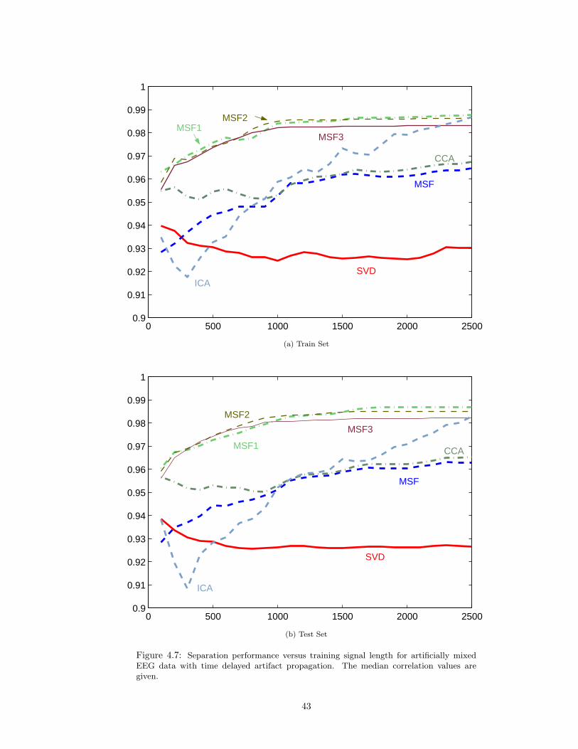
0 500 1000 1500 2000 25000.9

0.91

0.92

0.93

0.94

0.95

0.96

0.97

0.98

0.99

1

SVD ICA

MSF

CCA

MSF3 MSF1

MSF2

(a) Train Set

0 500 1000 1500 2000 25000.9

0.91

0.92

0.93

0.94

0.95

0.96

0.97

0.98

0.99

1

MSF

MSF1

MSF2

MSF3

ICA

CCA

SVD

(b) Test Set

Figure 4.7: Separation performance versus training signal length for artificially mixedEEG data with time delayed artifact propagation. The median correlation values aregiven.

43

In the analysis of classification algorithms it is necessary to have a validation set as well as a test

set. One of the test trials could be used as a validation set and the other as a training set. Once the

classifier has been trained on the two trials of the training set, each window in the validation set is

classified. This results in a classification rate for each of the modes. The mode resulting in the best

classification rates on the validation set is used to classify the test set. The resulting classification

rate is reported and used for comparison and analysis. The primary goal of this experiment is to

assess the effect of artifact removal on classification performance. So, a simpler method is used

to train and test the classifier. The windows in the train and test sets are recombined into two

groups: windows with eye blinks (EOG channel crosses 100 µV ) and windows without eye blinks.

Classification accuracy is reported on these two groups. This allows the effect of artifact removal

on these two groups of data to easily studied. Although this is not the correct method of testing

classification methods, it is more useful in comparing the effect of artifact removal methods on EEG

data.

Figure 4.8 shows the classification results for the 18 modes on the one-second windows that

contained eye blinks, detected using a 100 µV threshold, and those that did not. Classification

results are given for unfiltered data and data filtered with the seven different algorithms. The

measurement shown is the average percentage of windows correctly classified from both the training

and testing sets. In Mode 6, the sixth column, of Figure 4.8(a), the classification rate was 100% for

all filtering methods except the MSF with one lag. Similarly high performance is seen in Mode 6

of the windows without eye blinks, Figure 4.8(b), where all but the SVD and ICA have a 100%

classification rate. Mode 9 of Figure 4.8(a) is an example of filtering improving performance on

windows containing eye blinks. Classification was improved to 100% with data filtered by the MSF

with two and three lags.

Blink Mean Blink Max No Blink Mean No Blink MaxNONE 0.9810 1.0000 0.9724 1.0000SVD 0.9819 1.0000 0.9707 0.9991MSF 0.9765 1.0000 0.9710 0.9983MSF1 0.9770 1.0000 0.9709 0.9983MSF2 0.9779 1.0000 0.9731 1.0000MSF3 0.9752 1.0000 0.9729 1.0000CCA 0.9738 1.0000 0.9701 0.9983ICA 0.9806 1.0000 0.9715 0.9974

Table 4.4: The means and maximum values over the classification modes for each artifactremoval method and the unfiltered data.

It was noticed in preliminary studies that the MSF and ICA methods remove a pulse artifact

from the data used in this experiment. See Component 3 of Figure 2.7 on page 18 for an example

44

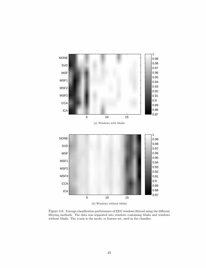
5 10 15

NONE

SVD

MSF

MSF1

MSF2

MSF3

CCA

ICA0.87

0.88

0.89

0.9

0.91

0.92

0.93

0.94

0.95

0.96

0.97

0.98

0.99

1

(a) Windows with blinks

5 10 15

NONE

SVD

MSF

MSF1

MSF2

MSF3

CCA

ICA0.87

0.88

0.89

0.9

0.91

0.92

0.93

0.94

0.95

0.96

0.97

0.98

0.99

1

(b) Windows without blinks

Figure 4.8: Average classification performance of EEG windows filtered using the differentfiltering methods. The data was separated into windows containing blinks and windowswithout blinks. The x-axis is the mode, or feature set, used in the classifier.

45

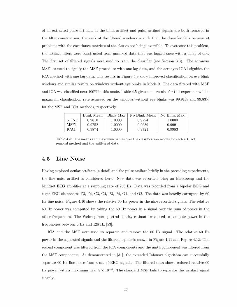
of an extracted pulse artifact. If the blink artifact and pulse artifact signals are both removed in

the filter construction, the rank of the filtered windows is such that the classifier fails because of

problems with the covariance matrices of the classes not being invertible. To overcome this problem,

the artifact filters were constructed from unmixed data that was lagged once with a delay of one.

The first set of filtered signals were used to train the classifier (see Section 3.3). The acronym

MSF1 is used to signify the MSF procedure with one lag data, and the acronym ICA1 signifies the

ICA method with one lag data. The results in Figure 4.9 show improved classification on eye blink

windows and similar results on windows without eye blinks in Mode 9. The data filtered with MSF

and ICA was classified near 100% in this mode. Table 4.5 gives some results for this experiment. The

maximum classification rate achieved on the windows without eye blinks was 99.91% and 99.83%

for the MSF and ICA methods, respectively.

Blink Mean Blink Max No Blink Mean No Blink MaxNONE 0.9810 1.0000 0.9724 1.0000MSF1 0.9752 1.0000 0.9689 0.9991ICA1 0.9874 1.0000 0.9721 0.9983

Table 4.5: The means and maximum values over the classification modes for each artifactremoval method and the unfiltered data.

4.5 Line Noise

Having explored ocular artifacts in detail and the pulse artifact briefly in the preceding experiments,

the line noise artifact is considered here. New data was recorded using an Electrocap and the

Mindset EEG amplifier at a sampling rate of 256 Hz. Data was recorded from a bipolar EOG and

eight EEG electrodes: F3, F4, C3, C4, P3, P4, O1, and O2. The data was heavily corrupted by 60

Hz line noise. Figure 4.10 shows the relative 60 Hz power in the nine recorded signals. The relative

60 Hz power was computed by taking the 60 Hz power in a signal over the sum of power in the

other frequencies. The Welch power spectral density estimate was used to compute power in the

frequencies between 0 Hz and 128 Hz [53].

ICA and the MSF were used to separate and remove the 60 Hz signal. The relative 60 Hz

power in the separated signals and the filtered signals is shown in Figure 4.11 and Figure 4.12. The

second component was filtered from the ICA components and the ninth component was filtered from

the MSF components. As demonstrated in [31], the extended Infomax algorithm can successfully

separate 60 Hz line noise from a set of EEG signals. The filtered data shows reduced relative 60

Hz power with a maximum near 5 × 10−5. The standard MSF fails to separate this artifact signal

cleanly.

46

5 10 15

NONE

MSF1

ICA1

0.87

0.88

0.89

0.9

0.91

0.92

0.93

0.94

0.95

0.96

0.97

0.98

0.99

(a) Windows with blinks

5 10 15

NONE

MSF1

ICA1

0.87

0.88

0.89

0.9

0.91

0.92

0.93

0.94

0.95

0.96

0.97

0.98

0.99

1

(b) Windows without blinks

Figure 4.9: Average classification performance of EEG windows filtered using the MSFand ICA methods with data lagged once with delay one. Eye blink and pulse artifactswere visually selected for removal.

47

EOG F3 F4 C3 C4 P3 P4 O1 O20

1

2

3

4

5x 10

−3

Rel

ativ

e 60

Hz

Pow

er

Figure 4.10: Relative 60 Hz power in a set of EEG signals.

1 2 3 4 5 6 7 8 9

Rel

ativ

e 60

Hz

Pow

er

1 2 3 4 5 6 7 8 90

1

2

3

4

5x 10

−3R

elat

ive

60H

z P

ower

Figure 4.11: Relative 60 Hz power in the ICA components and filtered data.

1 2 3 4 5 6 7 8 9

Rel

ativ

e 60

Hz

Pow

er

EOG F3 F4 C3 C4 P3 P4 O1 O20

1

2

3

4

5x 10

−3

Rel

ativ

e 60

Hz

Pow

er

Figure 4.12: Relative 60 Hz power in the MSF components and filtered data.

48

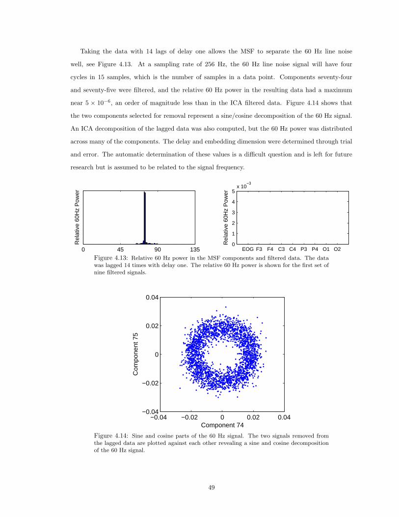
Taking the data with 14 lags of delay one allows the MSF to separate the 60 Hz line noise

well, see Figure 4.13. At a sampling rate of 256 Hz, the 60 Hz line noise signal will have four

cycles in 15 samples, which is the number of samples in a data point. Components seventy-four

and seventy-five were filtered, and the relative 60 Hz power in the resulting data had a maximum

near 5 × 10−6, an order of magnitude less than in the ICA filtered data. Figure 4.14 shows that

the two components selected for removal represent a sine/cosine decomposition of the 60 Hz signal.

An ICA decomposition of the lagged data was also computed, but the 60 Hz power was distributed

across many of the components. The delay and embedding dimension were determined through trial

and error. The automatic determination of these values is a difficult question and is left for future

research but is assumed to be related to the signal frequency.

0 45 90 135

Rel

ativ

e 60

Hz

Pow

er

EOG F3 F4 C3 C4 P3 P4 O1 O20

1

2

3

4

5x 10

−3

Rel

ativ

e 60

Hz

Pow

er

Figure 4.13: Relative 60 Hz power in the MSF components and filtered data. The datawas lagged 14 times with delay one. The relative 60 Hz power is shown for the first set ofnine filtered signals.

−0.04 −0.02 0 0.02 0.04−0.04

−0.02

0

0.02

0.04

Component 74

Com

pone

nt 7

5

Figure 4.14: Sine and cosine parts of the 60 Hz signal. The two signals removed fromthe lagged data are plotted against each other revealing a sine and cosine decompositionof the 60 Hz signal.

49

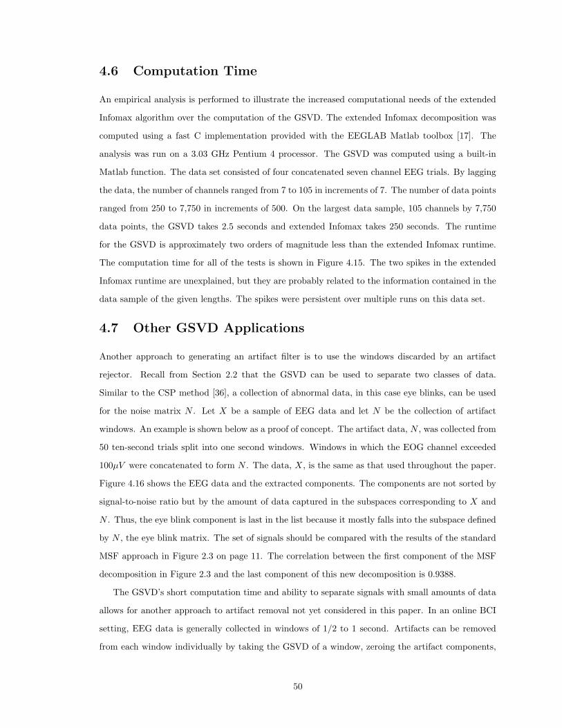
4.6 Computation Time

An empirical analysis is performed to illustrate the increased computational needs of the extended

Infomax algorithm over the computation of the GSVD. The extended Infomax decomposition was

computed using a fast C implementation provided with the EEGLAB Matlab toolbox [17]. The

analysis was run on a 3.03 GHz Pentium 4 processor. The GSVD was computed using a built-in

Matlab function. The data set consisted of four concatenated seven channel EEG trials. By lagging

the data, the number of channels ranged from 7 to 105 in increments of 7. The number of data points

ranged from 250 to 7,750 in increments of 500. On the largest data sample, 105 channels by 7,750

data points, the GSVD takes 2.5 seconds and extended Infomax takes 250 seconds. The runtime

for the GSVD is approximately two orders of magnitude less than the extended Infomax runtime.

The computation time for all of the tests is shown in Figure 4.15. The two spikes in the extended

Infomax runtime are unexplained, but they are probably related to the information contained in the

data sample of the given lengths. The spikes were persistent over multiple runs on this data set.

4.7 Other GSVD Applications

Another approach to generating an artifact filter is to use the windows discarded by an artifact

rejector. Recall from Section 2.2 that the GSVD can be used to separate two classes of data.

Similar to the CSP method [36], a collection of abnormal data, in this case eye blinks, can be used

for the noise matrix N . Let X be a sample of EEG data and let N be the collection of artifact

windows. An example is shown below as a proof of concept. The artifact data, N , was collected from

50 ten-second trials split into one second windows. Windows in which the EOG channel exceeded

100µV were concatenated to form N . The data, X, is the same as that used throughout the paper.

Figure 4.16 shows the EEG data and the extracted components. The components are not sorted by

signal-to-noise ratio but by the amount of data captured in the subspaces corresponding to X and

N . Thus, the eye blink component is last in the list because it mostly falls into the subspace defined

by N , the eye blink matrix. The set of signals should be compared with the results of the standard

MSF approach in Figure 2.3 on page 11. The correlation between the first component of the MSF

decomposition in Figure 2.3 and the last component of this new decomposition is 0.9388.

The GSVD’s short computation time and ability to separate signals with small amounts of data

allows for another approach to artifact removal not yet considered in this paper. In an online BCI

setting, EEG data is generally collected in windows of 1/2 to 1 second. Artifacts can be removed

from each window individually by taking the GSVD of a window, zeroing the artifact components,

50

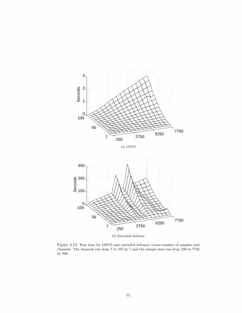
2502750

52507750

7

56

1050

1

2

3S

econ

ds

(a) GSVD

2502750

52507750

7

56

1050

150

300

450

Sec

onds

(b) Extended Infomax

Figure 4.15: Run time for GSVD and extended Infomax versus number of samples andchannels. The channels run from 7 to 105 by 7 and the sample sizes run from 250 to 7750by 500.

51

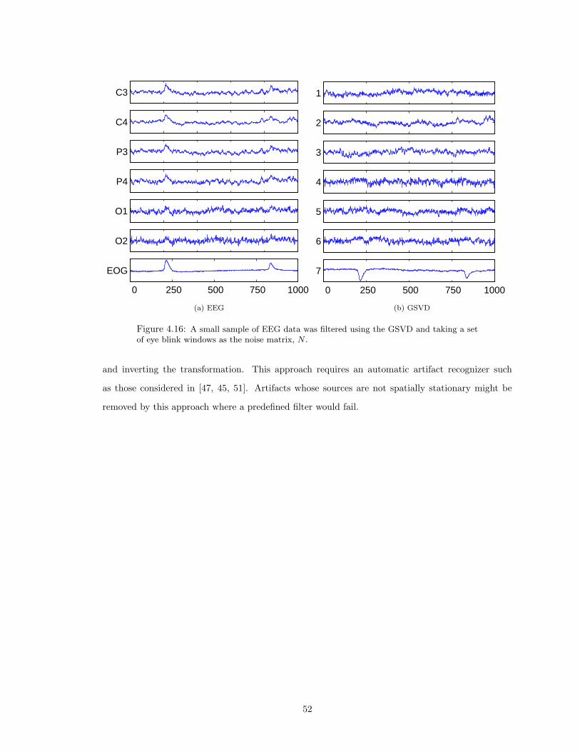
C3

C4

P3

P4

O1

O2

0 250 500 750 1000

EOG

(a) EEG

1

2

3

4

5

6

0 250 500 750 1000

7

(b) GSVD

Figure 4.16: A small sample of EEG data was filtered using the GSVD and taking a setof eye blink windows as the noise matrix, N .

and inverting the transformation. This approach requires an automatic artifact recognizer such

as those considered in [47, 45, 51]. Artifacts whose sources are not spatially stationary might be

removed by this approach where a predefined filter would fail.

52

Chapter 5

Conclusions

5.1 Discussion

Several experiments in the previous section explored the performance of different signal separa-

tion techniques on artificial data sets. The experiments reveal significant differences between the

maximum signal fraction (MSF) approach and the extended Infomax independent component anal-

ysis algorithm (ICA). The MSF signal separation method, combined with lagged data, successfully

separated the artificial mixtures using less data than Infomax. In Section 4.3, the methods were

compared on a data set into which a known artifact signal had been mixed and delayed at electrodes

in the back of the head. Performance of the methods was measured by correlation of the extracted

signal with the true artifact signal. The medians of this measure over several data sets fall into three

groups. The MSF with lags and ICA perform similarly when the full data set is used for training.

The MSF without lags and the canonical correlation analysis (CCA) method have close medians

that are less than the first group but greater than the SVD. When the length of the training signal

is halved, ICA falls into the MSF and CCA group.

By comparing classification of mental task data before and after artifact removal, a novel ap-

proach to comparing artifact removal methods was developed. The artifact removal focused on

ocular artifacts and classification was analyzed on two groups of data: the one second windows

with ocular artifacts and the set of windows without detectable ocular artifacts. Classification was

performed on 18 different feature sets which resulted in 18×2 classification values for each artifact

removal method. The SVD slightly improved average performance on the part of the data with

eye blinks; all other methods decreased average performance, although only slightly. A maximum

classification rate of 100% was achieved on the raw eye blink windows as well as in all of the filtered

sets. On the set of windows without eye blinks, the MSF with two and three lags improved average

performance and were the only methods, along with the unfiltered data, to achieve maximum classi-

53

fication of 100%. Performance was very similar among all methods, but this suggests that the MSF

with lagged observations may outperform the more computationally intensive ICA approach. The

key result of this experiment was that certain artifacts could be removed from a data set without

seriously decreasing classification performance.

Further experiments showed that the MSF was much easier to compute than the extended In-

fomax decomposition and that it could be used in other ways to remove artifacts. Much of the

previous work on artifact removal has focused on the extended Infomax method as an improvement

over principal component analysis. The MSF performs similarly to the Infomax method and better

in situations where limited data is available. The methods provide different characterizations of

EEG data. Infomax describes the data as a set of temporally independent signals, and MSF de-

composes the data as a set of sources ordered by signal-to-noise ratio. For certain artifacts, such

as eye blinks, it is important to remember that noise may be EEG data, since the artifact has high

amplitude. The combination of the MSF method and lagged data is novel in this context and im-

proves separation performance. Infomax can also be combined with lagged data, but it was found to

perform poorly on the artificial data experiments. It is possible that the artificial artifact signal was

split into two independent components and performed poorly because the methods were compared

by measuring the maximum correlation of one extracted signal with the true artifact signal. The

interaction between Infomax and lagged data is an open question.

5.2 Future Work

Many questions have been generated by the work presented in this thesis. The relation between

MSF analysis and ICA was only considered empirically, but a theoretical analysis might also provide

insight. A connection between the mutual information of a signal and a corrupted version of itself

and the signal-to-noise ratio of the corrupted signals exists for Gaussian signals [38]. Since ICA can

be seen as a maximization of the mutual information between a set of observations and a transformed

set of signals, this may be a useful place to begin the analysis. Mutual information, signal-to-noise

ratios, and canonical correlations all have relationships that might provide insight into the connection

between MSF and ICA through canonical correlation analysis.

The relationship between the SVD and the GSVD in terms of how much data is needed to

determine the transformations defined by these two methods is also an question that should be

answered. The SVD and GSVD are subspace methods and the subspaces defined by each method

have an effect on determining the transformations. The combination of lagging and GSVD was seen

to decrease the number of data points needed to define the MSF transformation. Lagging increases

54

the amount of information contained in each sample which may be the source of this phenomenon.

The ability to compute the MSF transform rapidly allows for the possibility of defining a unique

artifact filter for each window of EEG as it is collected. If the windows are large enough to completely

determine the filter then this approach may be superior to the static filter method. Certain artifacts,

such as muscle artifacts and external electrical signals, can be spatially non-stationary. This makes

them impossible to filter with a static filter unless the training data for the filter contains instances

of all the spatial locations of the artifact. Removing artifacts on a per window basis can overcome

this problem. Deciding on a minimum window size requires an answer to the question considered in

the previous paragraph.

A general question that should be more carefully considered is the necessity of artifact removal

in a BCI system. The classification experiments showed that removing artifacts did not improve

performance, but the experiments did give evidence that the classifier was successfully classifying

the underlying EEG data and not artifacts. More analysis into the effect of artifacts on mental task

classification will help to determine the importance of artifact removal in BCI systems.

55

REFERENCES

[1] H.D.I. Abarbanel. Analysis of Observed Chaotic Data. Springer-Verlag, New York, 1996.

[2] S. Amari. Natural gradient works efficiently in learning. Neural Computation, 10(2):251–276,1998.

[3] C. Anderson, E. Stolz, and S. Shamsunder. Multivariate autoregressive models for classifi-cation of spontaneous electroencephalogram during mental tasks. IEEE Transactions onBiomedical Engineering, 45(3):277–286, 1998.

[4] C.W. Anderson and M.J. Kirby. EEG subspace representations and feature selection for brain-computer interfaces. In Proceedings of the 1st IEEE Workshop on Computer Vision andPattern Recognition for Human Computer Interaction (CVPRHCI), Madison, Wisconsin,June 2003.

[5] A.J. Bell and T.J. Sejnowski. An information maximisation approach to blind separation andblind deconvolution. Neural Computation, 7(6):1129–1159, 1995.

[6] P. Berg and M. Scherg. Dipole models of eye activity and its application to the removal ofeye artifacts from the EEG and MEG. Clinical Physics and Physiological Measurements,12(Supplement A):49–54, 1991.

[7] W.T. Blume, M. Kaibara, and G.B. Young. Atlas of Adult Electroencephalography. LippincottWilliams and Wilkins, Philadelphia, 2002.

[8] M. Borga. Learning Multidimensional Signal Processing. PhD thesis, Linkoping University,S-581 83 Linkoping, Sweden, 1998.

[9] M. Borga, O. Friman, P. Lundberg, and H. Knutsson. A canonical correlation approach toexploratory data analysis in fMRI. In Proceedings of the ISMRM Annual Meeting, Honolulu,Hawaii, May 2002.

[10] M. Borga and H. Knutsson. A canonical correlation approach to blind source separation. Tech-nical Report LiU-IMT-EX-0062, Department of Biomedical Engineering, Linkping Univer-sity, 2001.

[11] J.-F. Cardoso. High-order contrasts for independent component anslysis. Neural Computation,11(1):157–192, 1999.

[12] M.T. Chu, R.E. Funderlic, and G.H. Golub. On a variational formulation of the generalizedsingular value decomposition. SIAM J. Matrix Anal. and App., 18(4):1082–1092, 1997.

[13] A. Cichocki and S. Vorobyov. Application of ICA for automatic noise and interference can-cellation in multisensory biomedical signals. In Proceedings of the Second InternationalWorkshop on ICA and BSS, pages 621–626, June 2000.

[14] R. J. Croft and R. J. Barry. EOG correction: Which regression should we use? Psychophysi-ology, 37:123–125, 2000.

[15] R. J. Croft and R. J. Barry. Removal of ocular artifact from the EEG: a review. ClinicalNeurophysiology, 30(1):5–19, 2000.

56

[16] Dr. Patti Davies. Personal communication. Occupational Therapy Department, Colorado StateUniversity.

[17] A. Delorme and S. Makeig. EEGLAB: an open source toolbox for analysis of single-trial eegdynamics including independent component analysis. Journal of Neuroscience Methods, InPress.

[18] G. Dornhege, B. Blankertz, and G. Curio. Speeding up classification of multi-channel brain-computer interfaces: Common spatial patterns for slow cortical potentials. In Proceedings ofthe 1st International IEEE EMBS Conference on Neural Engineering, pages 591–594, 2003.

[19] R. O. Duda and P. E. Hart. Pattern Classification and Scene Analysis. Wiley, New York, 1973.

[20] G.H. Golub and C.F. van Loan. Matrix Computations. Johns Hopkins University Press, Balti-more, 1996.

[21] G. Gratton, M.G. Coles, and E. Donchin. A new method for off-line removal of ocular artifact.Electroencephalography and Clinical Neurophysiology, 55:468–484, 1983.

[22] A.A. Green, M. Berman, P. Switzer, and M.D. Craig. A transformation for odering multispectraldata in terms of image quality with implications for noise removal. IEEE Transactions onGeoscience and Remote Sensing, 26(1):65–74, January 1988.

[23] S.A. Hillyard and R. Galambos. Eye-movement artifact in the CNV. Electroencephalographyand Clinical Neurophysiology, 28:173–182, 1970.

[24] R.A. Horn and C.R. Johnson. Matrix Analysis. Cambridge University Press, Cambridge, UK,1985.

[25] D.R. Hundley, M.J. Kirby, and M. Anderle. A solution procedure for blind signal separationusing the maximum noise fraction approach: algorithms and examples. In Proceedings ofthe Conference on Independent Component Analysis, pages 337–342, December 2001.

[26] D.R. Hundley, M.J. Kirby, and M. Anderle. Blind source separation using the maximum signalfraction approach. Signal Processing, 82:1505–1508, 2002.

[27] A. Hyvarinen, J. Karhunen, and E. Oja. Independent Component Analysis. John Wiley & Sons,New York, 2001.

[28] A. Hyvarinen and E. Oja. Independent component analysis: Algorithms and applications.Neural Networks, 13(4-5):411–430, 2000.

[29] H.H. Jasper. The ten-twenty electrode system of the international federation. Electroen-cephalography and Clinical Neurophysiology, 10:371–373, 1958.

[30] T-P. Jung, C. Humphries, M. Lee, V. Iragui, S. Makeig, and T. Sejnowski. Removing elec-troencephalographic artifacts: Comparison between ICA and PCA. In IEEE InternationalWorkshop on Neural Networks for Signal Processing, pages 63–72, 1998.

[31] T-P. Jung, C. Humphries, T.W. Lee, M.J. McKeown, V. Iragui, S. Makeig, and T.J. Sejnowski.Removing electroencephalographic artifacts by blind source separation. Psychophysiology,37:163–178, 2000.

[32] T-P. Jung, S. Makeig, M. Westerfield, J. Townsend, E. Courchesne, and T.J. Sejnowski. Re-moval of eye activity artifacts from visual event-related potentials in normal and clinicalsubjects. Clinical Neurophysiology, 111(10):1745–58, 2000.

[33] Z.A. Keirn and J.I. Aunon. A new mode of communication between man and his surroundings.IEEE Transactions on Biomedical Engineering, 37(12):1209–1214, December 1990.

[34] J.L. Kenemans, P. Molenaar, M.N. Verbaten, and J.L. Slangen. Removal of the ocular artifactfrom the EEG: a comparison of time and frequency domain methods with simulated andreal data. Psychophysiology, 28:114–121, 1991.

[35] M.J. Kirby and C.W. Anderson. Geometric analysis for the characterization of nonstationarytime-series. In E. Kaplan, J. Marsden, and K.R. Sreenivasan, editors, Springer AppliedMathematical Sciences Series Celebratory Volume for the Occasion of the 70th Birthday ofLarry Sirovich, chapter 8, pages 263–292. Springer-Verlag, 2003.

57

[36] Z.J. Koles. The quantitative extraction and topographic mapping of the abnormal componentsin the clinical EEG. Electroencephalography and Clinical Neurophysiology, 79:440–447, 1991.

[37] Z.J. Koles and A.C.K. Soong. EEG source localization: implementing the spatio-temoral de-composition approach. Electroencephalography and Clinical Neurophysiology, 107:343–352,1998.

[38] S. Kullback. Information Theory and Statistics. Wiley, New York, 1959.

[39] T.-W. Lee, M. Girolami, and T.J. Sejnowski. Independent component analysis using an ex-tended infomax algorithm for mixed sub-gaussian and super-gaussian sources. Neural Com-putation, 11(2):417–441, 1999.

[40] S. Makeig, A.J. Bell, T-P. Jung, and T.J. Sejnowski. Independent component analysis of elec-troencephalographic data. In D. Touretzky, M. Mozer, and M. Hasselmo, editors, Advancesin neural information processing systems, volume 8, pages 145–151, Cambridge, MA, 1996.The MIT Press.

[41] D.J. McFarland, L.M. McCane, S.V. David, and J.R. Wolpaw. Spatial filter selection for EEG-based communication. Electroencephalography and Clinical Neurophysiology, 103(3):386–394, 1997.

[42] J. Muller-Gerking, G. Pfurtscheller, and H. Flyvbjerg. Designing optimal spatial filters forsingle-trial EEG classification in a movement task. Clinical Neurophysiology, 110:787–798,1999.

[43] D.A. Overton and C. Shagass. Distribution of eye movement and eye blink potentials over thescalp. Electroencephalography and Clinical Neurophysiology, 27:546, 1969.

[44] M. Potter, N. Gadhok, and W. Kinsner. Separation performance of ICA on simulated EEGand ECG signals contaminated by noise. Canadian Journal of Electrical and ComputerEngineering, 27(3):123–127, July 2002.

[45] M. Rahalova, P. Sykacek, M. Koska, and G. Dorffner. Detection of the EEG artifacts by themeans of the (extended) Kalman filter. Measurement Science Review, 1(1):59–62, 2001.

[46] H. Ramoser, J. Muller-Gerking, and G. Pfurtscheller. Optimal spatial filtering of single trialEEG during imagined hand movement. IEEE Transactions on Rehabilitation Engineering,8(4):441–446, December 2000.

[47] A. Schlogl, P. Anderer, S.J. Roberts, M. Pregenzer, and G. Pfurtscheller. Artefact detectionin sleep EEG by the use of Kalman filtering. In Proceedings EMBEC’99, Part II, pages1648–1649, Vienna, Austria, November 1999.

[48] A.C.K. Soong and Z.J. Koles. Principal-component localization of the sources of the backgroundEEG. IEEE Transactions on Biomedical Engineering, 42(1):59–67, January 1995.

[49] F. Takens. Detecting strange attractors in turbulence. In D.A. Rand and L.S. Young, editors,Dynamical Systems and Turbulence, Lecture Notes in Mathematics 898. Springer-Verlag,New York, 1981.

[50] R. Verleger, T. Gasser, and J. Mocks. Correction of EOG artifacs in event-related potentials ofEEG: Aspects of reliability and validity. Psychophysiology, 19:472–480, 1982.

[51] S. Verobyov and A. Cichocki. Blind noise reduction fo multisensory signals using ICA andsubspace filtering, with application to EEG analysis. Biological Cybernetics, 86:293–303,2002.

[52] L. Vigon, M.R. Saatchi, J.E.W. Mayhew, and R. Fernandes. Quantitative evaulation of tech-niques for ocular artefact removal. IEE Proc.-Sci. Meas. Technol., 147(5), September 2000.

[53] P.D. Welch. The use of fast fourier transform for the estimation of power spectra: A methodbased on time averaging over short, modified periodograms. IEEE Transactions on AudioElectroacoustics, 15(2):70–73, June 1967.

58

[54] J.L. Whitton, F. Lue, and H. Moldofsky. A spectral method for removing eye-movement ar-tifacts from the EEG. Electroencephalography and Clinical Neurophysiology, 44:735–741,1978.

[55] J.C. Woestenburg, M.N. Verbaten, and J.L. Slangen. The removal of the eye-movement artifactfrom the EEG by regression analysis in the frequency domain. Biological Physiology, 16:127–147, 1983.

[56] J.R. Wolpaw, N. Birbaumer, W.J. Heetderks, D.J. McFarland, P.H. Peckham, G. Schalk,E. Donchin, L.A. Quatrano, C.J. Robinson, and T.M. Vaughan. Brain-computer interfacetechnology: A review of the first international meeting. IEEE Transactions on Rehabilita-tion Engineering, 8(2):164–173, June 2000.

[57] H. Zha. The Singular Value Decompositions Theory, Algorithms and Applications. PhD thesis,Pennsylvania State University, University Park, PA 16802, March 1993.

59

Appendix A

Common Spatial Patterns

This breif appendix is included to establish the connection between the common spatial patterns

(CSP) procedure and the generalized singular value decomposition (GSVD). Following [36], let Ap×n,

Bq×n be observations of two classes of data. Then the covariances are given by

Ra = A′A, and Rb = B′B

The sum of these covariance matrtices can be deomposed as

Rc ≡ Ra +Rb = UcλcUc′

and gives a whitening matrix

P = λ− 1

2

c Uc′.

Define two new matrices

Sa ≡ PRaP′ = (PA′)′(AP ) and Sb ≡ PRbP

′ = (PB′)′(BP ). (A.1)

The matrices, Sa and Sb have the same eigenvectors

Sa = QΨaQ′ and Sb = QΨbQ

′. (A.2)

The columns of the matrix W defined as

W = Q′P

are the common spatial patterns. The two data sets can be projected into the common spatial

pattern coordinates by AW ′ and BW ′.

The GSVD decomposes the two matrices as

A = UCX ′ and B = V SX ′,

60

with C2 + S2 = I and U and V orthogonal rectangular matrices [20]. Note that C2 = Ψa and

S2 = Ψb because of the relation between the GSVD of A and B and the generalized eigen-problem

associated with A′A and B′B [20]. It follows that

Ra = A′A = XC ′U ′UCX ′ = XCICX ′ = XC2X ′ (A.3)

and similarly for Rb. From equations A.1 and A.2 we can write Ra (similarly for Rb) as

Ra = P−1QΨaQ′P−T = (P−1Q)Ψa(P

−1Q)′ (A.4)

and then note that (A.3) and (A.4) imply

U = AX−TC−1 = AP ′Q−TΨ− 1

2

a .

Since Q is unitary, Q−T = Q and U = AP ′QΨ− 1

2

a so that U is equivalent to AW ′ within a scaling

of the columns.

61