Sierra Nevada-Southern Cascades (SNSC) Region Air ... · PDF fileSierra Nevada-Southern...

Sierra Nevada-Southern Cascades (SNSC) Region Air Contaminants Research and Monitoring Report

Prepared by:

Staci L. Simonich, Oregon State University

Leora Nanus, San Francisco State University

July 1, 2012

for the SNSC Steering Committee, including:

National Park Service; U.S. Forest Service; U.S. Fish & Wildlife Service; U.S. Geological Survey; USDA Natural Resources Conservation Board; U.S. Environmental Protection Agency; and the California Environmental Protection Agency, Air Resources Board, and Air Pollution Control Districts

ii

Contents Figures ........................................................................................................................................................ iv

Tables ......................................................................................................................................................... vii

1. Introduction ............................................................................................................................................. 1

1.1. Statement of Intent ............................................................................................................................. 1

1.2. Background ........................................................................................................................................ 1

1.3. Research Questions .......................................................................................................................... 2

1.4. Study Region ..................................................................................................................................... 3

1.5. Air Toxics Included in Report ............................................................................................................. 7

1.6. Air Masses Arriving to the SNSC Region .......................................................................................... 7

2. Air Toxics in the SNSC Region .............................................................................................................. 9

2.1. Current Use Pesticides (CUPs) ......................................................................................................... 9

2.2. Historic Use Pesticides (HUPs) ....................................................................................................... 15

2.3. Polychlorinated Biphenyls (PCBs) ................................................................................................... 37

2.4. Polycyclic Aromatic Hydrocarbons (PAHs) ...................................................................................... 38

2.5. Mercury ............................................................................................................................................ 39

2.6. Emerging Contaminants .................................................................................................................. 47

3. Ecosystem Indicators Used for Measuring Air Toxics in the SNSC Region ................................... 48

3.1. Atmospheric ..................................................................................................................................... 48

3.2. Aquatic ............................................................................................................................................. 49

3.3. Terrestrial ......................................................................................................................................... 50

4. Spatial Distribution of Air Toxics in Different Ecosystem Indicators .............................................. 54

4.1. Fish .................................................................................................................................................. 60

4.2. Surface Water .................................................................................................................................. 68

4.3. Snow ................................................................................................................................................ 76

4.4. Vegetation ........................................................................................................................................ 84

4.5. Air and Sediment ............................................................................................................................. 91

4.6. Amphibians ...................................................................................................................................... 94

5. Potential Ecosystem Impacts in the SNSC Region ........................................................................... 96

5.1. Bioaccumulation ............................................................................................................................... 96

5.2. Reproductive Disruption ................................................................................................................... 96

5.3. Immune Suppression ....................................................................................................................... 97

6. Recommendations ................................................................................................................................ 99

7. Outreach and Education..................................................................................................................... 100

8. Next Steps ............................................................................................................................................ 103

iii

8.1. Recommended Actions .................................................................................................................. 103

8.2. Suggested Methods ....................................................................................................................... 103

9. Conclusion ........................................................................................................................................... 105

10. Literature References ....................................................................................................................... 106

Appendix A. SNSC Toxics Funding Plan ............................................................................................. 114

Appendix B. SNSC Steering Committee .............................................................................................. 117

Appendix C. Laboratories used in previous studies .......................................................................... 118

Appendix D. Annotated Bibliography .................................................................................................. 119

Appendix E. Abbreviations ................................................................................................................... 123

iv

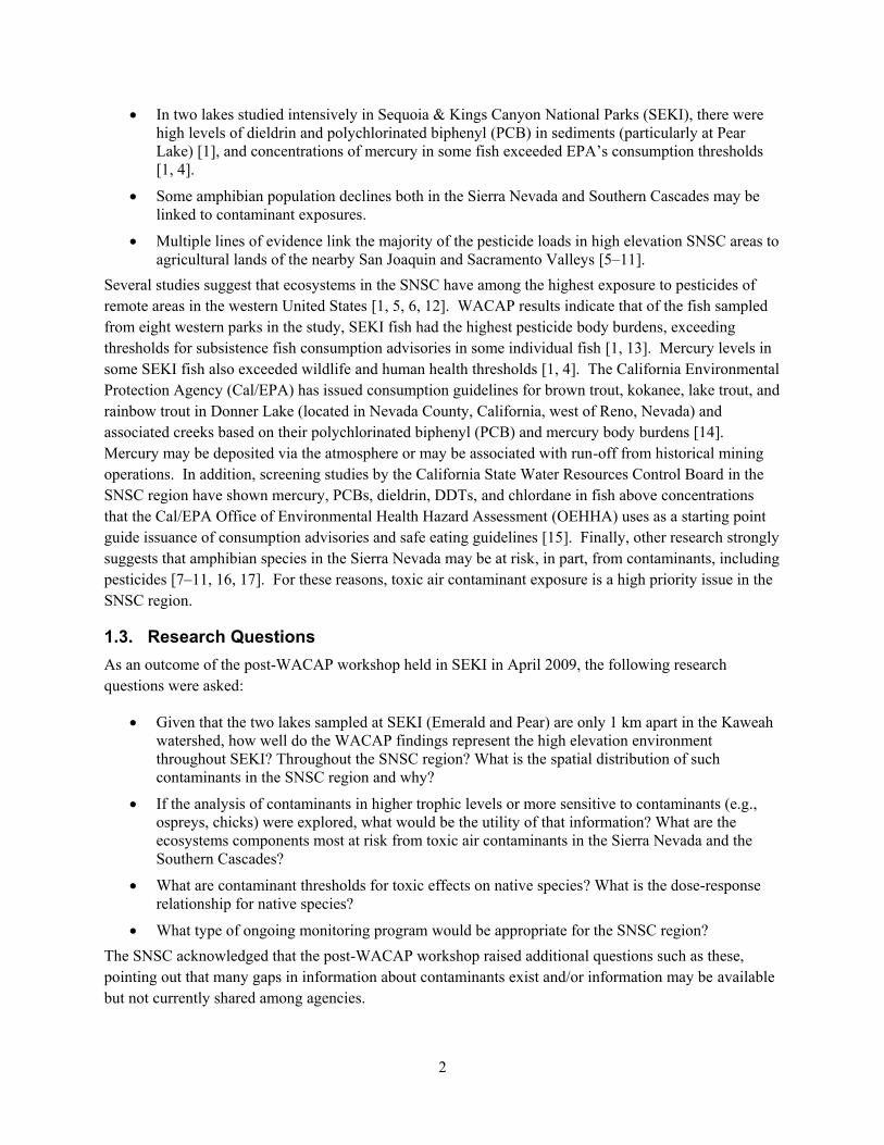
Figures Figure 1. Land ownership in the Sierra Nevada and Southern Cascades study region. .................... 4

Figure 2. Agricultural Pesticide Use in California by Township, 2009. ................................................ 5

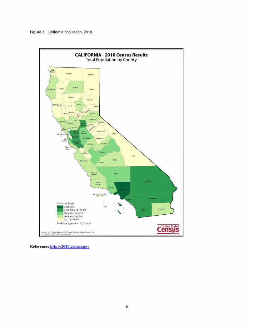
Figure 3. California population, 2010. ...................................................................................................... 6

Figure 4. WACAP 1, 5, and 10 day air mass back trajectories for SEKI [1]. ......................................... 8

Figure 5. Fish pesticide concentrations in western U.S. national parks, including SEKI, YOSE, and LAVO, from WACAP [1], compared to EPA human health thresholds [35]. ....................................... 19

Figure 5.1 Hexachlorobenzene (HCB) ................................................................................................... 19

Figure 5.2 Alpha-Hexachlorocyclohexane (α-HCH) .............................................................................. 20

Figure 5.3 Lindane (γ-HCH) ................................................................................................................... 20

Figure 5.4 Dacthal .................................................................................................................................. 21

Figure 5.5 Chlorpyrifos ........................................................................................................................... 21

Figure 5.6 Heptachlor epoxide ............................................................................................................... 22

Figure 5.7 Chlordanes ........................................................................................................................... 22

Figure 5.8 Dieldrin .................................................................................................................................. 22

Figure 5.9 Endosulfans .......................................................................................................................... 23

Figure 5.10 Mirex ................................................................................................................................... 24

Figure 5.11 pp’ DDE* ............................................................................................................................. 24

Figure 5.12 Methoxychlor ...................................................................................................................... 25

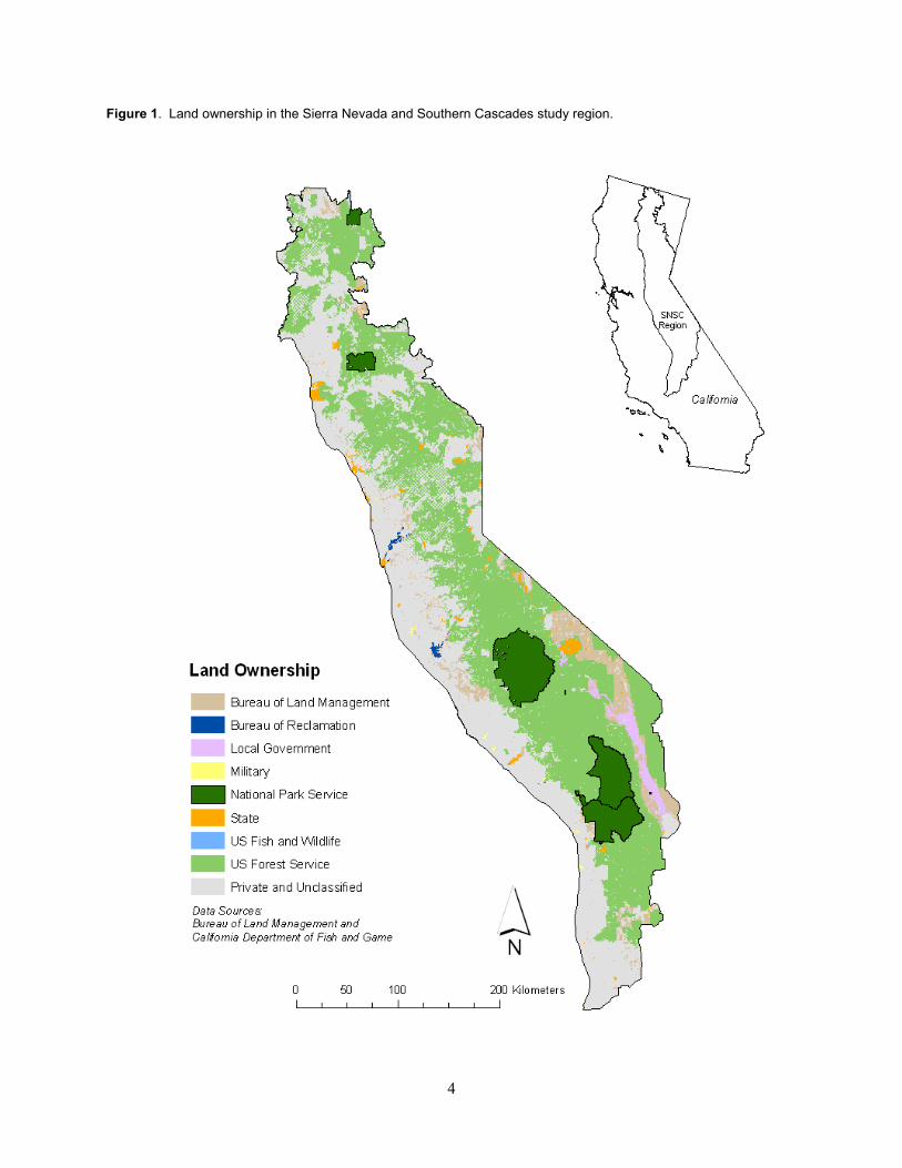
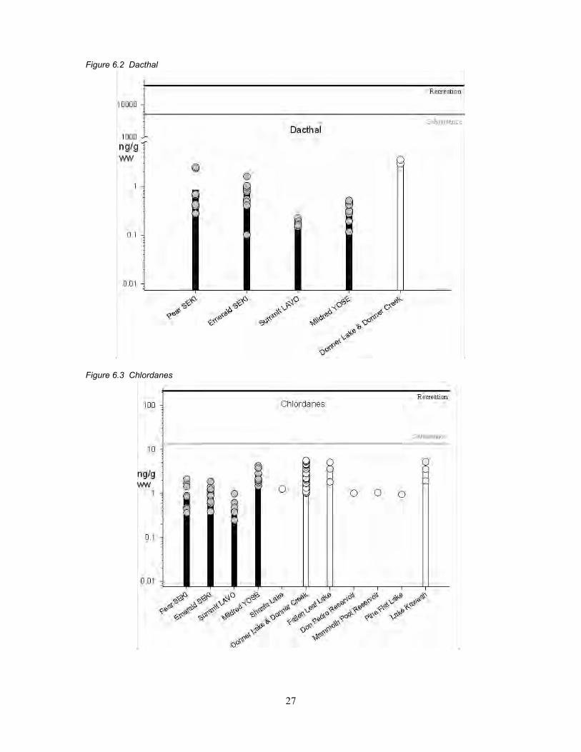
Figure 6. Fish pesticide and PCB concentrations in the SNSC region compared to human health thresholds [15, 35]. ................................................................................................................................... 26

Figure 6.1 Hexachlorobenzene (HCB) ................................................................................................... 26

Figure 6.2 Dacthal .................................................................................................................................. 27


Figure 6.4 Dieldrin .................................................................................................................................. 28

Figure 6.5.1 pp’ DDE ............................................................................................................................. 28

Figure 6.5.2 pp’ DDE ............................................................................................................................. 29

Figure 6.5.3 pp’ DDE ............................................................................................................................. 29

Figure 6.6.1 Total PCBs ......................................................................................................................... 30

Figure 6.6.2 Total PCBs ........................................................................................................................ 30

Figure 7. Fish HUP concentrations in western U.S. national parks (including SEKI, YOSE, and LAVO) measured by WACAP [1], compared to piscivorous wildlife health thresholds [48, 49]. ...... 31


Figure 7.2 Dieldrin .................................................................................................................................. 32

Figure 7.3 pp’ DDE ................................................................................................................................ 32

v

Figure 8. Fish HUP and PCB concentrations in the SNSC region [1, 15] compared to piscivorous wildlife health thresholds [48, 49]. .......................................................................................................... 33


Figure 8.2 Dieldrin .................................................................................................................................. 34

Figure 8.3.1 pp’ DDE ............................................................................................................................. 34

Figure 8.3.2 pp’ DDE ............................................................................................................................. 35

Figure 8.3.3 pp’ DDE ............................................................................................................................. 35



Figure 9. PAHs in snowpack, lichen, and surficial sediment of WACAP lake catchments. ............. 39

Figure 10. Average concentrations and fluxes of mercury across WACAP parks and media. ....... 41

Figure 11. Mercury concentrations in fish from western U.S. national parks [1], including SEKI, compared to human and piscivorous wildlife health thresholds [1, 4, 49]. ........................................ 42

Figure 12. Mercury concentrations in fish from the SNSC region [1, 15] compared to EPA human health and piscivorous wildlife thresholds [48, 49]. .............................................................................. 43

Figure 12.1 SEKI lakes vs. Medicine Lake–Stampede Reservoir ......................................................... 43

Figure 12.2 SEKI lakes vs. Bowman Lake–Lake Combie ..................................................................... 44

Figure 12.3 SEKI lakes vs. Loon Lake–Pinecrest.................................................................................. 44

Figure 12.5 SEKI lakes vs. Lake McSwain–Brite Valley Lake ............................................................... 45

Figure 13. Sampling locations and sample type for toxic air contaminants in the SNSC region (1990–2009). ............................................................................................................................................... 56

Figure 14. Sampling locations and sample type for toxic air contaminants at national parks in the SNSC region (1990–2009). ........................................................................................................................ 57

Figure 14.1 Yosemite National Park. ..................................................................................................... 57

Figure 14.3 Sequoia and Kings Canyon National Parks. ...................................................................... 58

Figure 14.4 Lassen Volcanic National Park. .......................................................................................... 59

Figure 15. Fish sampling sites in the SNSC region (2001–2009). ....................................................... 61

Figure 16. Total mercury concentrations in fish (2001–2009). ............................................................ 62

Figure 17. Polychlorinated Biphenyls (PCBs) detection in fish (2001–2009). ................................... 63

Figure 18. Chlorpyrifos detection in fish (2001–2009). ........................................................................ 64

Figure 19. Dieldrin concentrations in fish (2001–2009). ....................................................................... 65

Figure 20. Endosulfan detection in fish (2001–2009). .......................................................................... 66

Figure 21. Dacthal detection in fish (2001–2009). ................................................................................. 67

Figure 22. Surface water sampling sites (1997–2009). ......................................................................... 69

Figure 23. Endosulfan detection in surface water (1997–2009). ......................................................... 70

Figure 24. Chlorpyrifos concentration in surface water (1997–2009). ................................................ 71

Figure 25. Dieldrin detection in surface water (2002–2009). ................................................................ 72

vi

Figure 26. Dacthal detection in surface water (2002–2009). ................................................................ 73

Figure 27. Total mercury concentrations in surface water (1999–2009). ........................................... 74

Figure 28. Polychlorinated Biphenyls (PCBs) detection in surface water (2002–2009). .................. 75

Figure 29. Snow sampling sites (2002–2009). ....................................................................................... 77

Figure 30. Endosulfan concentrations in snow (2002–2009). .............................................................. 78

Figure 31. Dieldrin concentrations in snow (2002–2009). .................................................................... 79

Figure 32. Chlorpyrifos concentrations in snow (2002–2009). ............................................................ 80

Figure 33. Dacthal concentrations in snow (2002–2009). .................................................................... 81

Figure 34. Total mercury concentrations in snow (2002–2009). ......................................................... 82

Figure 35. Polychlorinated Biphenyls (PCBs) detection in snow (2002–2009). ................................. 83

Figure 36. Vegetation sampling sites (2002–2009). .............................................................................. 85

Figure 37. Endosulfan detection in vegetation (2002–2009). ............................................................... 86

Figure 38. Chlorpyrifos detection in vegetation (2002–2009). ............................................................. 87

Figure 39. Dieldrin detection in vegetation (2002–2009). ..................................................................... 88

Figure 40. Dacthal detection in vegetation (2002–2009). ..................................................................... 89

Figure 41. Polychlorinated Biphenyls (PCBs) detection in vegetation (2002–2009). ........................ 90

Figure 42. Air and dry deposition sampling sites (1990–2009). .......................................................... 92

Figure 43. Sediment sampling sites (2002–2009). ................................................................................ 93

Figure 44. Amphibian sampling sites (1997–2005). .............................................................................. 95

vii

Tables Table 1. The top current use pesticides (CUPs) by pounds used in California and evidence of atmospheric long-range transport, bioaccumulation, and effects on organisms as documented in the literature. ............................................................................................................................................. 11

Table 2. OEHHA human health Fish Contaminant Goals (FCGs) and Advisory Tissue Levels (ATLs) for fish concentrations of air toxics (ng/g wet weight) used by SWAMP [15] and the percent of SNSC region fish measured by SWAMP [15] and WACAP [1] that exceed the value. .................. 17

Table 3. EPA human health thresholds for subsistence and recreational fishing for fish concentrations of air toxics (ng/g wet weight) used by WACAP [1, 13] and the percent of SNSC region fish measured by SWAMP [15] and WACAP [1] that exceed the value. .................................. 18

Table 5. Recent mercury health thresholds for humans and piscivorous wildlife and percent of SNSC fish [1, 15] that exceed the threshold........................................................................................... 46

Table 6. Ecosystem indicators previously used for air toxics monitoring in the SNSC region. ..... 52

Table 7. Potential ecosystem impacts from air toxics in SNSC. ......................................................... 98

Table 8. Outreach products for communicating threats from contaminants in the SNSC. ........... 101

SNSC Toxics Steering Committee Agency Potential Funding Sources ............................................ 115

1

1. Introduction 1.1. Statement of Intent The objective of this report is to provide land managers and the public with spatial and temporal data and information about the threats of toxic air contaminants on sensitive receptors in the Sierra Nevada-Southern Cascades (SNSC) region. Sensitive receptors in the SNSC include lakes, streams, sediments, vegetation, amphibians, fish, wildlife, and humans. Report findings are based on maps of sensitive resources and existing contaminant data specifically regarding pesticides, industrial by-products, and mercury. SNSC resource managers can use the report as a foundation to address threats of contaminant deposition to SNSC ecosystems. This final report identifies:

1. The most sensitive ecological end points affected by toxic air contaminants; 2. Opportunities and recommendations for appropriately scaled research and monitoring of toxic air

contaminants; and 3. Outreach and education products to inform the public, agencies and regulators about the existing

threats to natural resources and human health resulting from the deposition and accumulation of toxic air contaminants.

The target audiences for this research and monitoring report are Federal land managers (National Park Service, NPS; US Forest Service, FS; US Fish & Wildlife Service, FWS) and regulatory agency staff (e.g., US Environmental Protection Agency, EPA), as well as staff of other agencies and Tribes in the State of California, including California Environmental Protection Agency (Cal/EPA), who are charged with preserving and protecting ecosystems, wildlife, and humans against exposure to toxic airborne contaminants. The results of this report will provide a framework for NPS, FS, and FWS managers to tier from when developing research and monitoring strategies to protect resources and people. The development and engagement of a multi-agency SNSC Air Contaminants Research and Monitoring Steering Committee (Steering Committee) ensures this project has broad land management and public applicability. The Steering Committee initiated development of this report so to better define the total suite of contaminants-related information that exists for the SNSC geographic area. This information will better equip land managers and policy makers for effective decision making.

1.2. Background The Western Airborne Contaminants Assessment Project (WACAP) was a six year study conducted by the NPS, the US Environmental Protection Agency (EPA),and other agency and university partners from 2001–2007 [1, 2]. The following summary statements, based on information provided by WACAP scientists and others involved in toxics research and monitoring in California [3], were agreed on at the post-WACAP Workshop held at Sequoia National Park in April 2009:

WACAP and other EPA, US Geological Survey (USGS), and State of California air contaminants research and monitoring projects have documented the presence and impact of airborne contaminants to ecosystems in the SNSC region.

Results suggest that high altitude ecosystems in this region have elevated levels of contaminants in fish, sediments, and conifer needles.

2

In two lakes studied intensively in Sequoia & Kings Canyon National Parks (SEKI), there were high levels of dieldrin and polychlorinated biphenyl (PCB) in sediments (particularly at Pear Lake) [1], and concentrations of mercury in some fish exceeded EPA’s consumption thresholds [1, 4].

Some amphibian population declines both in the Sierra Nevada and Southern Cascades may be linked to contaminant exposures.

Multiple lines of evidence link the majority of the pesticide loads in high elevation SNSC areas to agricultural lands of the nearby San Joaquin and Sacramento Valleys [5–11].

Several studies suggest that ecosystems in the SNSC have among the highest exposure to pesticides of remote areas in the western United States [1, 5, 6, 12]. WACAP results indicate that of the fish sampled from eight western parks in the study, SEKI fish had the highest pesticide body burdens, exceeding thresholds for subsistence fish consumption advisories in some individual fish [1, 13]. Mercury levels in some SEKI fish also exceeded wildlife and human health thresholds [1, 4]. The California Environmental Protection Agency (Cal/EPA) has issued consumption guidelines for brown trout, kokanee, lake trout, and rainbow trout in Donner Lake (located in Nevada County, California, west of Reno, Nevada) and associated creeks based on their polychlorinated biphenyl (PCB) and mercury body burdens [14]. Mercury may be deposited via the atmosphere or may be associated with run-off from historical mining operations. In addition, screening studies by the California State Water Resources Control Board in the SNSC region have shown mercury, PCBs, dieldrin, DDTs, and chlordane in fish above concentrations that the Cal/EPA Office of Environmental Health Hazard Assessment (OEHHA) uses as a starting point guide issuance of consumption advisories and safe eating guidelines [15]. Finally, other research strongly suggests that amphibian species in the Sierra Nevada may be at risk, in part, from contaminants, including pesticides [7–11, 16, 17]. For these reasons, toxic air contaminant exposure is a high priority issue in the SNSC region.

1.3. Research Questions As an outcome of the post-WACAP workshop held in SEKI in April 2009, the following research questions were asked:

Given that the two lakes sampled at SEKI (Emerald and Pear) are only 1 km apart in the Kaweah watershed, how well do the WACAP findings represent the high elevation environment throughout SEKI? Throughout the SNSC region? What is the spatial distribution of such contaminants in the SNSC region and why?

If the analysis of contaminants in higher trophic levels or more sensitive to contaminants (e.g., ospreys, chicks) were explored, what would be the utility of that information? What are the ecosystems components most at risk from toxic air contaminants in the Sierra Nevada and the Southern Cascades?

What are contaminant thresholds for toxic effects on native species? What is the dose-response relationship for native species?

What type of ongoing monitoring program would be appropriate for the SNSC region? The SNSC acknowledged that the post-WACAP workshop raised additional questions such as these, pointing out that many gaps in information about contaminants exist and/or information may be available but not currently shared among agencies.

3

1.4. Study Region The SNSC study region is shown in Figure 1 and includes Bureau of Land Management, USDA Forest Service (Eldorado, Inyo, Klamath, Lake Tahoe Basin, Lassen, Modoc, Plumas, Sequoia, Shasta-Trinity, Sierra, Stanislaus, Tahoe), National Park Service (SEKI, YOSE, and LAVO), US Fish & Wildlife Service refuges, California State Lands Commission, as well as other local public and private lands. Much of the SNSC region is adjacent to major agricultural areas, including the San Joaquin Valley (Figure 2), and areas with high population densities (Figure 3). Some air toxics, such as agricultural use pesticides, are used and emitted from agricultural areas, while other air toxics, such as polycyclic aromatic hydrocarbons, polychlorinated biphenyls, flame retardants, perfluorinated compounds and domestic use pesticides, are emitted from urban areas.

4

Figure 1. Land ownership in the Sierra Nevada and Southern Cascades study region.

5

Figure 2. Agricultural Pesticide Use in California by Township, 2009.

The color red indicates annual pound usage pesticide. The lightest red represents 0 to 3.4 pounds, medium red represents 3.4 to 68.4 pounds, and darkest red represents 68.4 + pounds used. (http://www.ehib.org/tool.jsp?tool_key=18)

http://www.ehib.org/tool.jsp?tool_key=18

6

Figure 3. California population, 2010.

Reference: http://2010.census.gov

http://2010.census.gov/

7

1.5. Air Toxics Included in Report This report focuses on the emission (regional and global), occurrence and toxicological relevance of organic air toxics and mercury with respect to the SNSC region. These air toxics were selected because they bioaccumulate in ecosystems and can cause toxicological effects. The organic air toxics include current use pesticides (CUPs), historic use pesticides (HUPs), emissions from incomplete combustion (polycyclic aromatic hydrocarbons, PAHs), PCBs, flame retardants (including polybrominated diphenyl ethers, PBDEs), and other emerging contaminants such as perfluorinated compounds (PFCs). These air toxics are emitted from both urban areas (PAHs, PCBs, PBDEs, PFCs, and domestic use pesticides) and rural areas (agricultural use pesticides).

1.6. Air Masses Arriving to the SNSC Region Figure 4 shows the clustering of 1, 5, and 10 day air mass back trajectories arriving at SEKI from 1998–2005 [1]. The trajectories shown in Figure 4 for SEKI represent the SNSC region because the model used (NOAA’s HYSPLIT model) has limited spatial resolution at the scale of the SNSC region [1]. The SNSC region is influenced by both regional (California, Oregon and Nevada) air masses and trans-Pacific air masses (Figure 4). The relative contribution of air toxics from regional air masses compared to trans-Pacific air masses is largely dependent on the strength of regional sources and proximity to the SNSC region. For example, the contribution of trans-Pacific sources to CUP and HUP deposition in SEKI seasonal snow pack was estimated to be 0–10% because of the close proximity of SEKI to the agriculturally intensive San Joaquin Valley and the episodic nature of trans-Pacific atmospheric transport [5, 6]. Jaffe et al. estimated that Asian anthropogenic emissions of mercury account for 7–20% of all mercury deposition in North America, in part because of its persistence in the atmosphere [18]. The relative contribution of local point sources of mercury in California (including cement plants [19], historical mining and wildfires [20–22]) is not well understood. However, the NPS is currently working to present EPA modeled data on the total (wet and dry) deposition of mercury to national parks (and the SNSC region), and to present USGS results regarding the risk of methylmercury in national park (and SNSC) ecosystems (http://www.nature.nps.gov/air/AQBasics/mercury.cfm). Finally, it has been estimated that Asian sources contributed 40–90% of the mineral dust in SEKI during July 2008 and 10–30% of the mineral dust in August and September 2008 [23].

http://www.nature.nps.gov/air/AQBasics/mercury.cfm

8

Figure 4. WACAP 1, 5, and 10 day air mass back trajectories for SEKI [1].

Each cluster represents the average transport pathway for a group of individual trajectories. Clusters are sorted from shortest (A) to longest (F) and correspond to the labeled cluster on the left-hand side of the figure. The bars represent the percent of trajectories in each cluster out of the total number of clusters calculated (2,922 from 1998–2005). The light blue color represents winter, light green represents spring, dark green represents summer and orange represents autumn. The dark blue dot is the percent of total precipitation that each cluster represents.

9

2. Air Toxics in the SNSC Region 2.1. Current Use Pesticides (CUPs) In general, CUPs have been designed and regulated to be less persistent and less mobile than historically used pesticides (HUPs). However, some CUPs have been measured in SNSC ecosystems (primarily SEKI, YOSE, and/or LAVO ecosystems), including: chlorpyrifos, chlorothalonil, trifluralin, malathion, simazine, propargite, dacthal, diazinon, endosulfan, parathion, methoxychlor, lindane, and triallate (Table 1) [1, 5–8, 13, 24–29]. In addition, some CUPs—pendimethalin, metolachlor, dimethoate, carbaryl, myclobutanil, propiconazole, linuron, methyl parathion, metribuzin, atrazine, phorate, disulfoton, dimethenamid, alachlor, ethion, terbufos, imidan, and cyanazine—have not been detected in the SNSC region but have been detected in other remote ecosystems. This is because: (1) research has not been conducted on these CUPs in the SNSC region, and/or (2) the pounds used in California were too low to result in measurable concentrations.

Table 1 shows the top CUPs applied in California in 2009, based on pounds used [30]. Table 1 also lists other CUPs that have been shown in the literature to undergo long-range atmospheric transport to remote ecosystems and their corresponding pounds used in California in 2009 [30]. Additional information in Table 1 includes, if the CUP was included as a WACAP analyte [1], if the CUP is included in the California Department of Pesticide Regulation air monitoring plan [30], and if there is evidence for atmospheric long-range transport of the CUP based on reported measurements of the CUP in remote ecosystems. CUPs used upwind of the SNSC region volatilize at the time of application and afterward, are transported and deposited to remote ecosystems [6]. CUPs are also released from terrestrial ecosystems during fires [31, 32]. The potential for CUPs to bioaccumulate in organisms, based on chemical structure and/or reports of measurement in organisms is also reported in Table 1. Finally, Table 1 contains information on CUPs expected to cause effects on organisms based on chemical structure, literature, or material safety data sheet, and information on the analytical method used to measure the CUP in the environment.

SNSC ecosystem studies outside of SEKI, YOSE, and LAVO have not generally included the measurement of CUPs (Section 4). However, endosulfan and dacthal were analyzed in fish as part of the Surface Water Ambient Monitoring Program (SWAMP), but concentrations were below the detection limit of the analytical methods used [15]. In contrast, endosulfan, dacthal, and chlorpyrifos were measured in fish above the detection limit in SEKI, YOSE, and LAVO by WACAP (Section 4 and Figure 5). This difference between the SWAMP and WACAP results is likely not because the SEKI, YOSE, and LAVO fish have higher CUP concentrations than the SWAMP fish, but because different laboratories made the respective measurements, using different analytical methods and detection limits.

Very few CUPs have been analyzed for in snow, surface water, and vegetation in the SNSC region outside of SEKI, YOSE, and LAVO (Section 4) even though both endosulfan and dacthal were measured above their detection limits in these matrices in SEKI, YOSE, and LAVO. Chlorpyrifos was measured both above and below the detection limit in snow, surface water, and vegetation in SEKI, YOSE, and LAVO. Figure 5 shows that the endosulfan, dacthal, and chlorpyrifos fish concentrations in SEKI, YOSE, and LAVO are similar to, or slightly higher than, western U.S. national parks in other geographic locations. This comparison helps put the range of SNSC fish CUP concentrations into perspective with other remote sites in the Western U.S. Figure 6 shows that the dacthal fish concentrations measured by

10

SWAMP in Donner Lake and Donner Creek are comparable to the concentrations measured in SEKI, YOSE, and LAVO fish. Only the SWAMP data above the detection limit is shown in Figure 6. Along with SNSC fish, endosulfan, chlorpyrifos, diazinon, and dacthal have been measured in SNSC amphibians, primarily in SEKI and YOSE [7, 8, 11, 17, 33, 34].

Although some CUPs are detected in fish collected from the SNSC region, their concentrations in fish do not currently exceed EPA guidelines for subsistence or recreational fishing by humans (Figures 5 and 6). Additionally, established wildlife contaminant health thresholds for most CUPs have not been developed [13, 35, 36]. In fact, the EPA recommends that only endosulfans, chlorpyrifos, diazinon, disulfoton, ethion, terbufos, and oxyfluorfen be measured in fish for evaluation against contaminant health thresholds because of their low bioaccumulation potential [36]. However, dated lake sediment cores from Pear and Emerald Lakes in SEKI and sediment cores from 19 lakes in YOSE, show that the deposition of CUPs to these ecosystems has continued to increase since they were first registered for use [1, 27] and that degradation, at least in the sediments, appears to be minimal. Therefore, it is possible that sediments are a source of CUPs to bioaccumulation pathways within these lakes.

Because the ecosystem impacts and environmental transport of a new pesticide cannot be fully known at the time of pesticide registration, new (and old) CUPs are a potential threat to SNSC ecosystems. However, if CUPS are identified in SNSC ecosystems and cause ecosystem effects, their use can be restricted. As a result, their concentrations in the environment (and associated effects) will decrease more rapidly than HUPs have because CUPs are generally less persistent in the environment.

Recommendations: Given the proximity of the SNSC region to major agricultural areas and the increased use of pesticides over time, it is recommended that CUPs and their breakdown products be included in future monitoring strategies, along with HUPs. CUP pounds used in California, literature reports of their presence in other remote ecosystems, and potential toxicological effects on organisms all require further study. Future analyte lists may warrant expansion to include more CUPs, especially those that have been measured in other remote ecosystems and are used in California. These CUPs include: pendimethalin, metolachlor, dimethoate, carbaryl, myclobutanil, propiconazole, linuron, methyl parathion, metribuzin, atrazine, phorate, disulfoton, dimethenamid, alachlor, ethion, terbufos, imidan, and cyanazine (Table 1).

Potential Outcome: If CUPs and their effects on organisms are identified in SNSC ecosystems, information regarding how measured concentrations compare to literature values, or information about direct effects in these ecosystems, can be used in regulatory processes to restrict the use of certain CUPs and to reduce their potential impact. A recent example of this is the use of WACAP data by EPA as contributing to the decision to phase-out the use of endosulfan in the U.S.

11

Table 1. The top current use pesticides (CUPs) by pounds used in California and evidence of atmospheric long-range transport, bioaccumulation, and effects on organisms as documented in the literature.

Other CUPs that have shown the potential for long-range transport are listed in the second half of the table, along with the pounds used in California in 2009. The pesticides (active ingredient) are listed in the table in order of amount used in California in 2009. ‘NI’ indicates no information is available. Pounds used for 2009 are the most recent data available [30]. ‘GC/MS’ indicates can be measured by gas chromatographic mass spectrometry. Reference numbers for the relevant literature are given in brackets. Open spaces in the table indicate the information was not assessed because the CUP does not undergo long-range transport.

Current Use Pesticide (CUP)

CAS Number Pounds Used in CA in 2009[30]

WACAP Analyte [1]?

Included in CA DPR Air Monitoring Plan?[37]

Evidence of Long Range Transport (LRT)?

If LRT–Potential for Bioaccumu-lation?

If LRT–Effects on Organisms?

If LRT–Analytical Method?

TOP CALIFORNIA CURRENT USE PESTICIDES BY POUNDS USED IN 2009 [30]:

Metam-Sodium 137-42-8 8,824,058 No No No NI NI NI

Glyphosate 1071-83-6 6,397,538 No No No NI NI NI

Chloropicrin 76-06-2 5,685,770 No Yes No NI NI NI

Potassium N-Methyldithiocarbamate 137-41-7 4,102,241 No No No NI NI NI

Propanil 709-98-8 1,904,607 No No No NI NI NI

Pendimethalin 40487-42-1 1,796,366 No No Svalbard Ice Cap[38] Yes Yes GC/MS

Chlorpyrifos 2921-88-2 1,235,481 Yes Yes

SEKI and YOSE and LAVO–WACAP[1] + others[5, 6, 8, 11, 13, 24, 26–29, 33, 35, 38–42]

Yes Yes GC/MS

Oxyfluorfen 42874-03-3 952,131 No Yes No NI NI NI

Paraquat Dichloride 1910-42-5 870,705 No No No NI NI NI

Chlorothalonil 37223-69-1 709,125 No Yes SEKI[28, 33, 40] + others[42] Yes Yes GC/MS

Maneb 12427-38-2 692,329 No No SEKI–[26] NI NI NI

Diuron 330-54-1 615,314 No Yes No NI NI NI

12



WACAP Analyte [1]?






Ziram 137-30-4 538,446 No No No NI NI NI

Trifluralin 1582-09-8 530,491 Yes Yes SEKI–WACAP + others[1, 28, 41, 42] [13, 26]

Yes Yes GC/MS

Malathion 121-75-5 528,196 Yes Yes SEKI–WACAP + others[1, 26, 28, 39] Yes Yes GC/MS

Oryzalin 19044-88-3 522,825 No Yes No NI NI NI

Glufosinate 77182-82-2 461,577 No No No NI NI NI

Simazine 122-34-9 415,136 Yes Yes SEKI –[25] Yes Yes GC/MS

Propargite 2312-35-8 380,106 No Yes SEKI –[25] Yes Yes GC/MS

Captan 133-06-2 325,464 No No No NI NI NI

Metolachlor 87392-12-9 304,751 No Yes Svalbard Ice Cap[43] + others[41, 42] Yes Yes GC/MS

Thiobencarb 28249-77-6 278,938 No No No NI NI NI

Permethrin 52645-53-1 278,229 No Yes No NI NI NI

Mancozeb 8018-01-7 277,572 No No No NI NI NI

Dimethoate 60-51-5 250,979 No Yes Svalbard Ice Cap[38, 43] Yes Yes GC/MS

Iprodione 36734-19-7 247,128 No Yes No NI NI NI

Methomyl 16752-77-5 220,860 No No No NI NI NI

MCPA 94-74-6 203,524 No No No NI NI NI

Ethephon 16672-87-0 202,123 No No No NI NI NI

Imidacloprid 138261-41-3 196,048 No No No NI NI NI

Chlorthal-Dimethyl Dacthal (DCPA) 1861-32-1 157,068 Yes Yes

SEKI and YOSE and LAVO–WACAP + others[1, 5, 6, 8, 13, 25, 27, 35, 40, 41]

Yes Yes GC/MS

Bifenthrin 82657-04-3 148,634 No No No NI NI NI

Methoxyfenozide 161050-58-4 142,924 No No No NI NI NI

13



WACAP Analyte [1]?






Boscalid 188425-85-6 142,393 No No No NI NI NI

Diazinon 333-41-5 141,366 Yes Yes SEKI-WACAP[1] + others[29] [11, 26, 28, 39, 43]

Yes Yes GC/MS

Phosmet 732-11-6 132,528 No Yes No NI NI NI

Carbaryl 63-25-2 130,981 No No ROMO and GLAC [40] Yes Yes GC/MS

Cyprodinil 121552-61-2 121,062 No No No NI NI NI

EPTC 759-94-4 116,031 Yes Yes No NI NI NI

Acephate 30560-19-1 112,251 No Yes No NI NI NI

Hexazinone 51235-04-2 111,310 No No No NI NI NI

Propamocarb 25606-41-1 105,879 No No No NI NI NI

OTHER CURRENT USE PESTICIDES WITH MEASURED LONG RANGE TRANSPORT:

Myclobutanil 88671-89-0 58,881 No No Canadian rain and air[42] Yes Yes GC/MS

Propiconazole 60207-90-1 55,009 No No Canadian rain and air[42] Yes Yes GC/MS

Linuron 330-55-2 50,523 No No Canadian rain and air[42] Yes Yes GC/MS

Endosulfan 115-29-7 41,724 Yes Yes

SEKI and YOSE and LAVO– WACAP[1] + others[5, 6, 8, 11, 13, 25–28, 35, 40, 42]

Yes Yes GC/MS

Methyl Parathion 298-00-0 25,357 Yes No Austfonna Ice Core Yes Yes GC/MS

Metribuzin 21087-64-9 22,770 Yes No Devon ice cap-Arctic[41] Yes Yes GC/MS

Atrazine 1912-24-9 22,187 Yes No ROMO and GLAC–Mast et al.[40] + others[42–44] Yes Yes GC/MS

Phorate 298-02-2 15,291 No No Devon ice cap-Arctic[41] Yes Yes GC/MS

Disulfoton 298-04-4 8,330 No No Svalbard Ice Cap[38, 43] Yes Yes GC/MS

Dimethenamid 87674-68-8 1,528 No No Canadian rain and air[42] Yes Yes GC/MS

Alachlor 15972-60-8 246 Yes No Svalbard Ice Cap[38, 43] Yes Yes GC/MS

Parathion 56-38-2 117 Yes No Sierra Nevada Mtns.[29] Yes Yes GC/MS

14



WACAP Analyte [1]?






Ethion 563-12-2 28 Yes No Austfonna ice core Yes Yes GC/MS

Methoxychlor 72-43-5 8 Yes No

SEKI and YOSE and LAVO- WACAP[1, 13] + others[35]; Devon ice cap-Arctic[41]

Yes Yes GC/MS

Lindane 58-89-9 8 Yes No SEKI–WACAP[1] + others[5, 6, 28, 41] Yes Yes GC/MS

Prometon 1610-18-0 1 Yes No No NI NI NI

Terbufos 13071-79-9 NI No No Svalbard Ice Cap[38] Yes Yes GC/MS

Imidan 732-11-6 NI No No Svalbard Ice Cap[38, 43] Yes Yes GC/MS

Etridiazole 2593-15-9 NI Yes No No NI NI NI

Pebulate 1114-71-2 NI Yes No No NI NI NI

Triallate 2303-17-5 NI Yes No SEKI-WACAP[1, 13] Yes Yes GC/MS

Cyanazine 21725-46-2 NI Yes No Isle Royale, Lake Superior[44] Yes Yes GC/MS

Acetochlor 34256-82-1 NI Yes No No NI NI NI

Propachlor 1918-16-7 NI Yes No No NI NI NI

15

2.2. Historic Use Pesticides (HUPs) Historic use pesticides (HUPs), including chlordanes, dieldrin, DDTs, nonachlors, heptachlors, and hexachlorobenzene, have been measured in fish throughout the SNSC region but in surface water, snow, vegetation and sediment primarily in SEKI, YOSE and LAVO ecosystems (Section 4) [1, 5–8, 13, 25, 27, 45]. Along with SNSC fish, DDTs, chlordanes, HCHs, and nonachlors, have been measured in SNSC amphibians [7, 8, 11, 17, 33, 34, 46]. These same HUPs were measured in fish collected throughout the SNSC ecosystem by SWAMP [15].

Figure 5 shows that the hexachlorobenzene, alpha-HCH, heptachlor epoxide, chlordane, dieldrin, mirex, DDE, and methoxychlor fish concentrations in SEKI, YOSE, and LAVO are similar to, or slightly higher than, other western U.S. national parks. This comparison helps put the range of SNSC fish HUP concentrations into perspective with other remote sites in the Western U.S. Figure 6 shows that, in cases where fish HUP concentrations were above the detection limit, the HCB, chlordane, dieldrin, and DDE concentrations in SWAMP fish collected from the SNSC region were comparable to the fish concentrations in SEKI, YOSE, and LAVO. As with CUPs, only the SWAMP fish data above the detection limit are shown in Figure 6. The HUP detection limits for the SWAMP fish are likely higher than the detection limits for the WACAP fish in SEKI, YOSE, and LAVO because different laboratories and analytical methods were used.

Studies indicate that HUPs continue to be deposited to the SNSC region through wet deposition (snow and rain) [5, 6, 27] and dry deposition, but that this deposition has decreased since these pesticides were banned from use in the U.S. [1]. As part of WACAP, Hageman and Simonich et al. determined that there is a high correlation between the HUP concentrations and fluxes in seasonal snowpack in Western U.S. national parks and the historic cropland intensity within 150 km of the parks [5, 6]. Using a series of different western U.S. national parks, with different surrounding cropland intensities and measured HUP and CUP concentrations in seasonal snowpack, they determined that 95–100% of the HUPs (and CUPs) deposited to SEKI are the result of regional atmospheric transport surrounding SEKI and not trans-Pacific atmospheric transport from Asia [5, 6]. For HUPs, this occurs because of their continued persistence in surrounding agricultural soils from past use, followed by their volatilization from these soils, and their transport and deposition to remote SNSC ecosystems [5, 6]. HUPs are also released from terrestrial ecosystems during forest fires [31, 32]

Some individual fish collected from Emerald Lake and Pear Lake in SEKI, Summit Lake in LAVO, Mildred Lake in YOSE, and SWAMP fish from the SNSC region had DDE and dieldrin concentrations that exceeded EPA human health guidelines for subsistence and recreational fishing [13, 35]. Screening studies by the California State Water Resources Control Board in the SNSC region (i.e., SWAMP) have shown dieldrin, DDTs, and chlordane in fish above concentrations that the Cal/EPA Office of Environmental Health Hazard Assessment (OEHHA) uses as a starting point to determine whether to issue consumption advisories and safe eating guidelines [15]. Figure 5 shows the fish concentrations of dieldrin, DDTs, and chlordane as measured in western U.S. national parks (including parks from the SNSC region) with respect to human health thresholds for these HUPs. Figure 6 shows both WACAP and SWAMP data for the fish HUP concentration in the SNSC region.

Table 2 shows different human health thresholds for chlordanes, DDTs, and dieldrin in fish as chosen by the California OEHHA and used by SWAMP [15, 47]. Table 2 also indicates the percentage of SNSC region fish measured by SWAMP and WACAP that exceeded each threshold. The Fish Contaminant

16

Goals (FCGs) are described as “estimates of contaminant levels in fish that pose no significant health risk to humans consuming sport fish at a standard consumption rate of one serving per week (or eight ounces–before cooking–per week, or 32 g/day), prior to cooking, over a lifetime and can provide a starting point for OEHHA to assist other agencies that wish to develop fish tissue-based criteria with a goal toward pollution mitigation or elimination” [15, 47]. FCGs are used to prevent consumers from being exposed to more than the daily reference dose for non-carcinogens or to a risk level greater than 1 x 10-6 for carcinogens (not more than one additional cancer case in a population of 1 million people consuming fish at the given consumption rate over a lifetime) [15, 47]. The OEHHA Advisory Tissue Levels (ATLs) are provided for three servings per week, two servings per week, and for no consumption.

Table 3 shows the human health thresholds for chlordanes, DDTs, and dieldrin for recreational and subsistence fish consumers as chosen by EPA and used by WACAP [1, 13]. Table 3 also shows the percentage of SNSC region fish measured by SWAMP and WACAP that exceeded each threshold. Contaminant specific health thresholds are calculated fish contaminant concentrations that will likely lead to contaminant consumption exceeding EPA Integrated Risk Information System (IRIS) reference doses or acceptable cancer risk levels for individual contaminants only. These threshold calculations assume typical recreation or subsistence fish consumption [1, 13]. EPA default recreational (17.5 g of fish per day) and subsistence fishing consumption rates (142 g of fish per day), adult body mass (70 kg individuals), and acceptable risk levels (lifetime excess cancer risk of 1:100,000) are used to calculate the contaminant health thresholds and lake specific advisory fish consumption limits [1, 13]. Contaminant health thresholds for recreational fishing are adjusted to account for differences between the measured whole fish semi-volatile organic compound (SOC) concentrations and likely exposure in trimmed and cooked fish fillets by increasing the contaminant threshold by 32%, to account for an average 32% reduction in air toxics exposure estimated to be achieved by trimming and cooking using EPA recommended values. Subsistence fishing health thresholds are not adjusted for reductions from whole fish SOC concentrations since subsistence consumption patterns are highly variable and often include the whole fish (soups, stews, etc.)[1, 13].

In comparing Tables 2 and 3, it is clear that the OEHHA and EPA human health thresholds are not the same. However, the OEHHA FCG’s are similar to the EPA subsistence fishing consumption patterns assuming additive cancer risk and the OEHHA’s Advisory Tissue Levels (ATL’s) for three servings per week are similar to the EPA recreational fishing consumption patterns assuming additive cancer risk. In general, the EPA thresholds are slightly lower (and more protective) than the OEHHA’s values. As a result, the percentage of fish measured by SWAMP and WACAP in the SNSC region that exceed a given health threshold is slightly larger when EPA health thresholds are used. For example the percentage of fish exceeding the EPA dieldrin threshold for subsistence fishing consumption patterns is 44% and it is 40% for the OEHHA dieldrin FCG. However, if one government agency within the SNSC region uses the EPA dieldrin threshold for subsistence fish consumption and another government agency within the SNSC region uses the OEHHA dieldrin ATL for two servings per week, the exceedance varies from 44% for the former threshold to 11% for the latter.

Finally, there are no established HUP wildlife health thresholds for the SNSC region, including for piscivorous wildlife. WACAP used chlordane, dieldrin, and DDT thresholds for piscivorous wildlife known to occur in the majority of national parks (kingfisher, mink, and river otter) and where nonlethal end points were used as indicators of a negative effect [1, 13, 48, 49]. Corresponding thresholds for piscivorous fish have not been established. Figure 7 shows the fish concentrations of chlordane, dieldrin,

17

and DDTs with respect to these wildlife thresholds for western U.S. national parks, for comparison to the SNSC region. Figure 8 shows the data for the SNSC region only, including SWAMP and WACAP data. In addition, Table 4 shows the percentage of SNSC fish measured to date that exceed various piscivorous wildlife thresholds for chlordanes, DDTs, and dieldrin. No individual fish exceeded the dieldrin wildlife thresholds. However, approximately 10% of the individual fish measured in the SNSC region exceeded the chlordane and DDT thresholds for Kingfisher.

Recommendations: HUPs continue to be deposited in SNSC ecosystems as a result of past use (and continued persistence) in agricultural soils in California. Although, the deposition of HUPs to the SNSC region is not expected to increase in the future, future studies that continue to measure HUPs in fish collected from the SNSC region would ensure that the public is aware of any potential risks associated with consumption of fish from this region. In addition, comparing and analyzing the differences between the OEHHA and EPA fish consumption thresholds for the protection of human health is recommended. Given the sometimes significant differences between the human health thresholds, it is important that consistent thresholds be applied by government agencies throughout the SNSC region. At a minimum, it is recommended that the human health thresholds employed by an agency be disclosed to the public when data are reported. Additionally, it is important that consistent wildlife health thresholds are developed and utilized by government agencies throughout the SNSC region. In cooperation with the Steering Committee, wildlife toxicology experts can apply existing data on the wildlife species present in the SNSC region and documented health impacts from contaminants to develop wildlife health thresholds for the region. This work would improve understanding of HUPs on wildlife and improve the ability of agencies to protect sensitive populations.

Potential Outcome: If HUP concentrations exceed human and wildlife health thresholds, the public can be notified of the potential risk and steps can be taken to minimize wildlife exposure.

Table 2. OEHHA human health Fish Contaminant Goals (FCGs) and Advisory Tissue Levels (ATLs) for fish concentrations of air toxics (ng/g wet weight) used by SWAMP [15] and the percent of SNSC region fish measured by SWAMP [15] and WACAP [1] that exceed the value.

*SWAMP data only.

Air Toxic OEHHA Fish Contaminant Goals (ng/g)

% of SNSC Fish exceed-ing

OEHHA Advisory Tissue Level (3 servings / week) (ng/g)


OEHHA Advisory Tissue Level (2 servings / week) (ng/g)


OEHHA Advisory Tissue Level (no consump-tion) (ng/g)


Chlordanes 5.6 0.56 190 0 280 0 560 0 DDTs 21 0 520 0 1000 0 2100 0 Dieldrin 0.46 40.0 15 11.1 23 11.1 46 6.1 PCBs* 3.6 2.5* 21 0.5* 42 0.2* 120 0* Mercury 220 52.5 70 81.1 150 62.2 440 5.8

18

Table 3. EPA human health thresholds for subsistence and recreational fishing for fish concentrations of air toxics (ng/g wet weight) used by WACAP [1, 13] and the percent of SNSC region fish measured by SWAMP [15] and WACAP [1] that exceed the value.

Air Toxic EPA additive cancer risk–subsistence fishing (ng/g)

% of SNSC Fish exceeding

EPA additive cancer risk-recreational fishing (ng/g)


Chlordanes 14 0.56 170 0

DDTs 14 0.56 170 0

Dieldrin 0.31 44 3.7 18.9

Table 4. Piscivorous wildlife risk values for consuming fish (ng/g wet weight) [48] and the percent of SNSC region fish measured by SWAMP [15] and WACAP [1] that exceed the value.

Air Toxic Mink (ng/g) % of SNSC Fish exceeding

Kingfisher (ng/g)


Chlordanes 830 0 4.5 9.5 DDTs 360 0 20 9.7 Dieldrin 20 0 360 0 PCBs 130 0 440 0

19

Figure 5. Fish pesticide concentrations in western U.S. national parks, including SEKI, YOSE, and LAVO, from WACAP [1], compared to EPA human health thresholds [35].

Top of bar indicates the mean concentration of all fish measured in the lake and the symbols represent the concentrations of individual fish. The bars for SEKI, LAVO and YOSE are highlighted in black because they are within the SNSC region. HUPs include HCB (hexachlorobenzene), α-HCH (alpha-hexachlorocyclohexane), chlordanes, dieldrin, mirex, heptachlor epoxide, and DDE. CUPS include γ-HCH (lindane), dacthal, chlorpyrifos, endosulfans, and methoxychlor. Contaminant thresholds are from EPA: The recreation threshold is based on consumption of 17.5 g of fish per day and the subsistence threshold is based on consumption of 142 g of fish per day. “*” indicates non-detects. Fish PCB concentrations are not included because of the limited number of PCB congeners measured in fish from national parks as part of WACAP.

Figure 5.1 Hexachlorobenzene (HCB)

Pear SEKI

Emerald SEKI

Mills ROMO

LonePine ROMO

LP19 MORA

Golden MORA

Hoh OLYM

PJ OLYM

Oldman GLAC

Snyder GLAC

McLeod DENA

Wonder DENA

Matcharak G

AAR

Burial NOAT

Tanada WRST

Copper WRST

Sand GRSD

Summit LAVO

Mildred YOSE

Dream ROMO

Haynach ROMO

Haiyaha Lake

Lone Pine ROMO

Nanita ROMO

Spirit Lake ROMO

Ypsilon ROMO

ng/gww

0.01

0.1

1

10

Recreation

Subsistence

HCB

20

Figure 5.2 Alpha-Hexachlorocyclohexane (α-HCH)

* *

Lake, Park

Pear SEKI

Emerald SEKI

Mills ROMO

LonePine ROMO

LP19 MORA

Golden MORA

Hoh OLYM

PJ OLYM

Oldman GLAC

Snyder GLAC

McLeod DENA

Wonder DENA

Matcharak G

AAR

Burial NOAT

Tanada WRST

Copper WRST

Sand GRSD

Summit LAVO

Mildred YOSE

Dream ROMO

Haynach ROMO

Haiyaha Lake

Lone Pine ROMO

Nanita ROMO

Spirit Lake ROMO

ng/gww

0.01

0.1

1

10 Recreation

Subsistence

-HCH

Figure 5.3 Lindane (γ-HCH)

Pear SEKI

Emerald SEKI

Mills ROMO

LonePine ROMO

LP19 MORA

Golden MORA

Hoh OLYM

PJ OLYM

Oldman GLAC

Snyder GLAC

McLeod DENA

Wonder DENA

Matcharak G

AAR

Burial NOAT

Tanada WRST

Copper WRST

Sand GRSD

Summit LAVO

Mildred YOSE

Dream ROMO

Haynach ROMO

Haiyaha Lake

Lone Pine ROMO

Nanita ROMO

Spirit Lake ROMO

Ypsilon ROMO

ng/gww

0.001

0.01

0.1

100

1000 Recreation

Subsistence

*** * * * * * * **

-HCH

21

Figure 5.4 Dacthal

Pear SEKI

Emerald SEKI

Mills ROMO

LonePine ROMO

LP19 MORA

Golden MORA

Hoh OLYM

PJ OLYM

Oldman GLAC

Snyder GLAC

McLeod DENA

Wonder DENA

Matcharak G

AAR

Burial NOAT

Tanada WRST

Copper WRST

Sand GRSD

Summit LAVO

Mildred YOSE

Dream ROMO

Haynach ROMO

Haiyaha Lake

Lone Pine ROMO

Nanita ROMO

Spirit Lake ROMO

Ypsilon ROMO

ng/gww

0.01

0.1

1

1000

10000

Recreation

SubsistenceDacthal

Figure 5.5 Chlorpyrifos

Pear SEKI

Emerald SEKI

Mills ROMO

LonePine ROMO

LP19 MORA

Golden MORA

Hoh OLYM

PJ OLYM

Oldman GLAC

Snyder GLAC

McLeod DENA

Wonder DENA

Matcharak G

AAR

Burial NOAT

Tanada WRST

Copper WRST

Sand GRSD

Summit LAVO

Mildred YOSE

Dream ROMO

Haynach ROMO

Haiyaha Lake

Lone Pine ROMO

Nanita ROMO

Spirit Lake ROMO

Ypsilon ROMO

ng/gww

0.001

0.01

0.1

1

1000

10000 Recreation

Subsistence

* *

Chlorpyrifos

22

Figure 5.6 Heptachlor epoxide

* * * * * * * * * *

Pear SEKI

Emerald SEKI

Mills ROMO

LonePine ROMO

LP19 MORA

Golden MORA

Hoh OLYM

PJ OLYM

Oldman GLAC

Snyder GLAC

McLeod DENA

Wonder DENA

Matcharak G

AAR

Burial NOAT

Tanada WRST

Copper WRST

Sand GRSD

Summit LAVO

Mildred YOSE

Dream ROMO

Haynach ROMO

Haiyaha Lake

Lone Pine ROMO

Nanita ROMO

Spirit Lake ROMO

Ypsilon ROMO

ng/gww

0.01

0.1

1

10Recreation

Subsistence

Heptachlor epoxide

Figure 5.7 Chlordanes

Pear SEKI

Emerald SEKI

Mills ROMO

LonePine ROMO

LP19 MORA

Golden MORA

Hoh OLYM

PJ OLYM

Oldman GLAC

Snyder GLAC

McLeod DENA

Wonder DENA

Matcharak G

AAR

Burial NOAT

Tanada WRST

Copper WRST

Sand GRSD

Summit LAVO

Mildred YOSE

Dream ROMO

Haynach ROMO

Haiyaha Lake

Lone Pine ROMO

Nanita ROMO

Spirit Lake ROMO

Ypsilon ROMO

ng/gww

0.01

0.1

1

10

100Recreation

Subsistence

Chlordanes

Figure 5.8 Dieldrin

23

Pear SEKI

Emerald SEKI

Mills ROMO

LonePine ROMO

LP19 MORA

Golden MORA

Hoh OLYM

PJ OLYM

Oldman GLAC

Snyder GLAC

McLeod DENA

Wonder DENA

Matcharak G

AAR

Burial NOAT

Tanada WRST

Copper WRST

Sand GRSD

Summit LAVO

Mildred YOSE

Dream ROMO

Haynach ROMO

Haiyaha Lake

Lone Pine ROMO

Nanita ROMO

Spirit Lake ROMO

ng/gww

0.01

0.1

1

10

Recreation

Subsistence

Dieldrin

Figure 5.9 Endosulfans

Pear SEKI

Emerald SEKI

Mills ROMO

LonePine ROMO

LP19 MORA

Golden MORA

Hoh OLYM

PJ OLYM

Oldman GLAC

Snyder GLAC

McLeod DENA

Wonder DENA

Matcharak G

AAR

Burial NOAT

Tanada WRST

Copper WRST

Sand GRSD

Summit LAVO

Mildred YOSE

Dream ROMO

Haynach ROMO

Haiyaha Lake

Lone Pine ROMO

Nanita ROMO

Spirit Lake ROMO

Ypsilon ROMO

ng/gww

0.01

0.1

1

1000

10000Recreation

Subsistence

Endosulfans

24

Figure 5.10 Mirex

Pear SEKI

Emerald SEKI

Mills ROMO

LonePine ROMO

LP19 MORA

Golden MORA

Hoh OLYM

PJ OLYM

Oldman GLAC

Snyder GLAC

McLeod DENA

Wonder DENA

Matcharak G

AAR

Burial NOAT

Tanada WRST

Copper WRST

Sand GRSD

Summit LAVO

Mildred YOSE

Dream ROMO

Haynach ROMO

Haiyaha Lake

Lone Pine ROMO

Nanita ROMO

Spirit Lake ROMO

Ypsilon ROMO

ng/gww

0.01

0.1

1

10

100 Recreation

Subsistence

* *

Mirex

Figure 5.11 pp’ DDE*

Pear SEKI

Emerald SEKI

Mills ROMO

LonePine ROMO

LP19 MORA

Golden MORA

Hoh OLYM

PJ OLYM

Oldman GLAC

Snyder GLAC

McLeod DENA

Wonder DENA

Matcharak G

AAR

Burial NOAT

Tanada WRST

Copper WRST

Sand GRSD

Summit LAVO

Mildred YOSE

Dream ROMO

Haynach ROMO

Haiyaha Lake

Lone Pine ROMO

Nanita ROMO

Spirit Lake ROMO

Ypsilon ROMO

ng/gww

0.01

0.1

1

10

100Recreation

Subsistence

pp DDE

*pp’ DDE is the form of DDT most often found in fish. It is generally abbreviated as DDE throughout this report.

25

Figure 5.12 Methoxychlor

Pear SEKI

Emerald SEKI

Mills ROMO

LonePine ROMO

LP19 MORA

Golden MORA

Hoh OLYM

PJ OLYM

Oldman GLAC

Snyder GLAC

McLeod DENA

Wonder DENA

Matcharak G

AAR

Burial NOAT

Tanada WRST

Copper WRST

Sand GRSD

Summit LAVO

Mildred YOSE

Dream ROMO

Haynach ROMO

Haiyaha Lake

Lone Pine ROMO

Nanita ROMO

Spirit Lake ROMO

Ypsilon ROMO

ng/gww

0.01

0.1

1

10

1000

10000 Recreation

Subsistence

* * * * **

Methoxychlor

26

Figure 6. Fish pesticide and PCB concentrations in the SNSC region compared to human health thresholds [15, 35].

Top of bar indicates the mean concentration of all fish measured in the lake and the symbols represent the concentrations of individual fish. The bars for SEKI, LAVO and YOSE are highlighted in black and the remaining bars are fish concentrations from reference [15] for SWAMP sites within the SNSC region. Only SWAMP data above the detection limit was plotted. The fish DDE and PCB concentrations are shown in multiple graphs because many of the SWAMP sites had fish DDE and PCB concentrations above the detection limit. Compounds include HCB (hexachlorobenzene), chlordanes, dieldrin, DDE, dacthal, and PCBs [15]. The fish PCB concentrations from SEKI, YOSE, and LAVO are not compared to the SWAMP PCB fish concentrations because of measurement differences. Only SWAMP PCB data above the detection limit are plotted. PCB thresholds are from OEHHA (as in Table 2 – FCG (4 ng/g) and ATLs (3 servings/week: 21 ng/g; 2 servings/week: 42 ng/g; no consumption: 120 ng/g)), and the other contaminant thresholds are from EPA (recreation threshold based on consumption of 17.5 g of fish per day; subsistence threshold based on consumption of 142 g of fish per day).

Figure 6.1 Hexachlorobenzene (HCB)

27

Figure 6.2 Dacthal


28

Figure 6.4 Dieldrin

Figure 6.5.1 pp’ DDE

29



30

Figure 6.6.1 Total PCBs


31

Figure 7. Fish HUP concentrations in western U.S. national parks (including SEKI, YOSE, and LAVO) measured by WACAP [1], compared to piscivorous wildlife health thresholds [48, 49].

Top of bar indicates the mean concentration of all fish measured in the lake and the symbols represent the concentrations of individual fish. The bars for SEKI, LAVO and YOSE are highlighted in black because they are within the SNSC region. HUPs include chlordanes, dieldrin, and DDE.


32

Figure 7.2 Dieldrin

Figure 7.3 pp’ DDE

33

Figure 8. Fish HUP and PCB concentrations in the SNSC region [1, 15] compared to piscivorous wildlife health thresholds [48, 49].

Top of bar indicates the mean concentration of all fish measured in the lake and the symbols represent the concentrations of individual fish. The bars for SEKI, LAVO and YOSE are highlighted in black and the remaining bars are fish concentrations from reference [15] for SWAMP sites within the SNSC region. Only SWAMP data above the detection limit was plotted. The fish DDE and PCB concentrations are shown in multiple graphs because many of the SWAMP sites had fish DDE and PCB concentrations above the detection limit. Compounds include chlordanes, dieldrin, DDE and PCBs [15]. The fish PCB concentrations from SEKI, YOSE, and LAVO are not compared to the SWAMP PCB fish concentrations because of measurement differences (see text).


34

Figure 8.2 Dieldrin


35



36



37

2.3. Polychlorinated Biphenyls (PCBs) Similar to pesticides, PCBs are ubiquitous in SNSC ecosystems and have been measured in the same matrices as HUPs, including fish, snow, vegetation, sediments, and amphibians (Section 4) [8, 33]. Other than in fish, PCBs have not been measured in the SNSC region outside of SEKI, YOSE, and LAVO (Section 4).

PCBs have been banned from manufacture in the U.S. since 1979 but continue to persist primarily in urban areas due to their presence in transformers, other electrical equipment, and paints. While PCBs continue to be deposited in SNSC ecosystems (measured in precipitation in SEKI and YOSE [1, 27]), it is unclear if the deposition of PCBs is increasing, decreasing, or staying the same. Sediment cores collected from lakes in SEKI and YOSE show mixed results with regard to surficial sediment layers being higher or lower in PCB concentrations than lower sediments within the same core [1, 27]. This may be a result of measurements near the detection limit of the analytical method or due to the slow release of PCBs from sources in California. In general, PCB emissions are not expected to increase in the future because of their ban. However, PCBs are released from terrestrial ecosystems during forest fires [31, 32]. PCBs have not been shown to undergo significant trans-Pacific atmospheric transport because there was limited use of PCBs in Asia compared to the rest of the northern hemisphere [1, 13, 27, 31, 33, 50–52].

PCBs have been measured by SWAMP in fish collected throughout the SNSC region and in SEKI, YOSE, and LAVO fish by WACAP at concentrations above and below the detection limit (Section 4). Forty-four PCB congeners were measured in the SWAMP fish, while 7 PCB congeners were measured in WACAP fish. Because of this measurement difference, the SWAMP fish PCB concentrations should not be directly compared to the WACAP fish PCB concentrations. SWAMP PCB fish concentrations are shown in Figure 6, Figure 8, and Table 2. WACAP PCB fish concentrations are not shown.

The California EPA has issued consumption guidelines for brown trout, kokanee, lake trout, and rainbow trout in Donner Lake and associated creeks based on their concentrations of PCBs [14]. In addition, screening studies by the California State Water Resources Control Board in the SNSC region have shown PCBs in fish above concentrations that the OEHHA uses as a starting point to determine whether to issue consumption advisories and safe eating guidelines [15].

Table 2 shows the fish tissue PCB concentrations for the two types of human health thresholds for concern chosen by the OEHHA and used by SWAMP: FCGs and ATLs [15, 47]. Table 2 also shows the percentage of SNSC region fish measured by SWAMP that exceeded the listed threshold. These data are also presented in Figures 6.6.1 and 6.6.2. Because a limited number of PCBs were targeted for measurement in WACAP, the EPA human health thresholds for PCBs were not used in WACAP.

Finally, there are no established PCB health thresholds for piscivorous wildlife in the SNSC region. Figures 8.4.1 and 8.4.2 show the SWAMP fish PCB concentrations (above the detection limit) in comparison to total PCB health thresholds for kingfisher, mink, and river otter [1, 13, 48, 49]. In addition, Table 4 shows the percentage of SWAMP fish that exceed the piscivorous wildlife thresholds for PCBs. No individual fish exceeded the PCB piscivorous wildlife thresholds.

Recommendations: PCBs continue to be deposited in SNSC ecosystems primarily due to their past use in urban areas in California. Although the deposition of PCBs to the SNSC region is not expected to increase in the future, it is recommended that future studies continue measuring PCBs in fish collected

38

from the SNSC region. This work will ensure that the public is aware of any potential risks associated with consumption of fish from this region. In addition, it is recommended that the SNSC Steering Committee select consistent wildlife and human health thresholds for use within the SNSC region and lands. It is important that these consistent thresholds are applied by different government agencies throughout the SNSC region.

Potential Outcome: If PCB concentrations in fish collected from the SNSC region exceed consumption guidelines, the public can be notified of the potential risk. The SNSC Steering Committee may be able to guide the development of wildlife thresholds for PCBs that can be used to assess wildlife risk in the future.

2.4. Polycyclic Aromatic Hydrocarbons (PAHs) PAHs are emitted from all combustion sources (e.g., autos, wood burning, power plants) and continue to be emitted in the U.S., although U.S. emissions have decreased in the past 25 years. China is now the world’s largest emitter of PAHs and the episodic trans-Pacific atmospheric transport of PAHs to the U.S. West Coast has been documented (primarily in the Spring) [32, 53, 54]. Nevertheless, trans-Pacific transport contributes less than 10% annually, and PAHs emitted within California are likely the major source of PAHs to the SNSC region. PAHs are also emitted during forest fires [31, 32].

PAHs are likely ubiquitous in SNSC ecosystems but have only been explicitly studied at SEKI, YOSE, and LAVO in snow, fish, sediment, amphibians, and vegetation (Section 4) [1, 8, 13, 55]. PAHs were measured in YOSE lake water using semi-permeable membrane devices (SPMDs) [27] and low PAH concentrations have been measured in SNSC amphibians [8]. PAHs were not measured in fish collected by SWAMP.

Figure 9 shows that the PAH flux and concentrations in SEKI, YOSE, and LAVO are comparable to other western national parks studied in WACAP, with the exception of Glacier National Park (GLAC) [1, 55]. GLAC had unusually high PAH concentrations that are attributed to the presence of a local aluminum smelter [1, 55]. Dated sediment cores from Pear and Emerald Lakes in SEKI showed that PAH deposition to these lakes has been decreasing over the past 25 years [1].

Although PAHs are potent carcinogens, they are metabolized and hence do not bioaccumulate and biomagnify to the degree that hydrophobic CUPs, HUPs, and PCBs do in higher organisms, such as fish and amphibians. The PAH concentrations in SEKI, YOSE, and LAVO do not currently exceed any human consumption guidelines [13] and piscivorous wildlife health thresholds for PAHs have not been established. However, PAHs can have varying effects on wildlife including inhibited reproduction, delayed emergence, liver abnormalities, immune system impairments, and mortality.

Recommendations: PAHs continue to be deposited in SNSC ecosystems primarily due to current emissions from combustion sources (autos, trucks, wood burning, forest fires, and power plants) within California, with a small contribution from trans-Pacific transport. The deposition of PAHs to the SNSC region will increase in the future if the population of California increases and PAH emissions from autos, trucks, wood burning and power plants do not decrease. Because the PAH concentrations in SNSC fish do not currently exceed human health thresholds, it is recommended that future studies include PAHs in their measurements only when potential new PAH point sources are identified or the contribution of urban areas to pollutants in the SNSC region is of concern.

39

Potential Outcome: Not routinely measuring PAHs in the SNSC region may free up funds for the measurement of other emerging air toxics of interest.

Figure 9. PAHs in snowpack, lichen, and surficial sediment of WACAP lake catchments.

Sampling sites in the SNSC region (SEKI) are shown with the darkest bars. Snowpack samples were not collected at Hoh Lake and PJ Lake because of reduced snowpack. ‘nd’ indicates not detected and ‘nm’ indicates not measured because samples were not available for collection. Snowpack data for all sampling locations were collected in 2003. Lichen and sediment samples were collected from Emerald, Pear, Mills, and Lone Pine Lake in 2003; McLeod, Wonder, Matcharak, and Burial Lake in 2004; and LP19, Golden, Hoh, PJ, Oldman, and Snyder Lake in 2005. (Figure taken from reference [55].)

2.5. Mercury Mercury (including methylmercury) is ubiquitous in SNSC ecosystems [1, 4, 14, 15, 56–60] and has been measured in fish, amphibians, surface water, snow, vegetation, and sediment in SNSC ecosystems [1, 5–8, 13, 15, 25, 27, 45, 61] (Section 4). Other than mercury measurements in fish collected by SWAMP, mercury has not been extensively measured in other matrices outside of SEKI, YOSE, and LAVO (Section 4). A study measuring over 300 fish samples collected from the Tuolumne River watershed (YOSE) for mercury and testing air samples for mercury has been funded by the City of San Francisco and is currently underway. A separate NPS/USGS study is also analyzing mercury in fish from SEKI, YOSE, LAVO, and other western national parks. In addition, songbirds are being assessed for mercury from YOSE in collaboration with the Biodiversity Research Institute. Songbirds are important indicators of mercury in the terrestrial ecosystem.

The mercury concentrations in lichen, snow, fish, and surficial sediment in SEKI are comparable to U.S. national parks in other geographic locations (Figures 10 and 11). This comparison helps put the range of

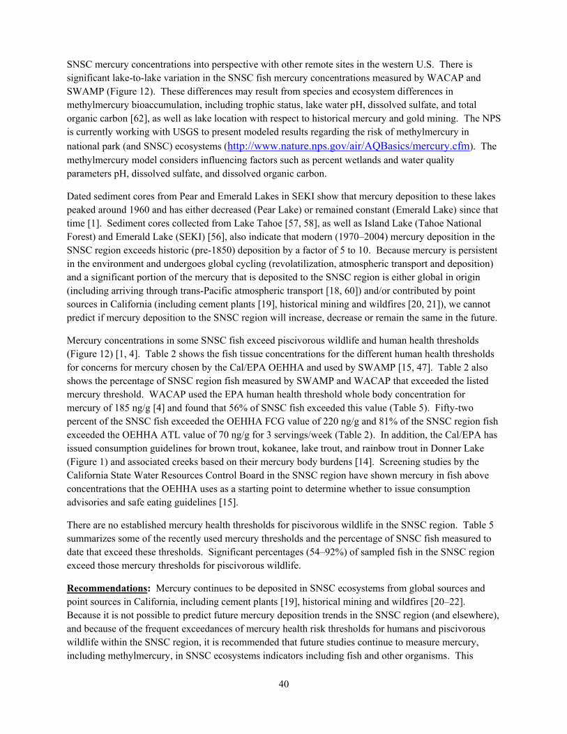
40

SNSC mercury concentrations into perspective with other remote sites in the western U.S. There is significant lake-to-lake variation in the SNSC fish mercury concentrations measured by WACAP and SWAMP (Figure 12). These differences may result from species and ecosystem differences in methylmercury bioaccumulation, including trophic status, lake water pH, dissolved sulfate, and total organic carbon [62], as well as lake location with respect to historical mercury and gold mining. The NPS is currently working with USGS to present modeled results regarding the risk of methylmercury in national park (and SNSC) ecosystems (http://www.nature.nps.gov/air/AQBasics/mercury.cfm). The methylmercury model considers influencing factors such as percent wetlands and water quality parameters pH, dissolved sulfate, and dissolved organic carbon.

Dated sediment cores from Pear and Emerald Lakes in SEKI show that mercury deposition to these lakes peaked around 1960 and has either decreased (Pear Lake) or remained constant (Emerald Lake) since that time [1]. Sediment cores collected from Lake Tahoe [57, 58], as well as Island Lake (Tahoe National Forest) and Emerald Lake (SEKI) [56], also indicate that modern (1970–2004) mercury deposition in the SNSC region exceeds historic (pre-1850) deposition by a factor of 5 to 10. Because mercury is persistent in the environment and undergoes global cycling (revolatilization, atmospheric transport and deposition) and a significant portion of the mercury that is deposited to the SNSC region is either global in origin (including arriving through trans-Pacific atmospheric transport [18, 60]) and/or contributed by point sources in California (including cement plants [19], historical mining and wildfires [20, 21]), we cannot predict if mercury deposition to the SNSC region will increase, decrease or remain the same in the future.

Mercury concentrations in some SNSC fish exceed piscivorous wildlife and human health thresholds (Figure 12) [1, 4]. Table 2 shows the fish tissue concentrations for the different human health thresholds for concerns for mercury chosen by the Cal/EPA OEHHA and used by SWAMP [15, 47]. Table 2 also shows the percentage of SNSC region fish measured by SWAMP and WACAP that exceeded the listed mercury threshold. WACAP used the EPA human health threshold whole body concentration for mercury of 185 ng/g [4] and found that 56% of SNSC fish exceeded this value (Table 5). Fifty-two percent of the SNSC fish exceeded the OEHHA FCG value of 220 ng/g and 81% of the SNSC region fish exceeded the OEHHA ATL value of 70 ng/g for 3 servings/week (Table 2). In addition, the Cal/EPA has issued consumption guidelines for brown trout, kokanee, lake trout, and rainbow trout in Donner Lake (Figure 1) and associated creeks based on their mercury body burdens [14]. Screening studies by the California State Water Resources Control Board in the SNSC region have shown mercury in fish above concentrations that the OEHHA uses as a starting point to determine whether to issue consumption advisories and safe eating guidelines [15].

There are no established mercury health thresholds for piscivorous wildlife in the SNSC region. Table 5 summarizes some of the recently used mercury thresholds and the percentage of SNSC fish measured to date that exceed these thresholds. Significant percentages (54–92%) of sampled fish in the SNSC region exceed those mercury thresholds for piscivorous wildlife.

Recommendations: Mercury continues to be deposited in SNSC ecosystems from global sources and point sources in California, including cement plants [19], historical mining and wildfires [20–22]. Because it is not possible to predict future mercury deposition trends in the SNSC region (and elsewhere), and because of the frequent exceedances of mercury health risk thresholds for humans and piscivorous wildlife within the SNSC region, it is recommended that future studies continue to measure mercury, including methylmercury, in SNSC ecosystems indicators including fish and other organisms. This

http://www.nature.nps.gov/air/AQBasics/mercury.cfm

41

research will ensure that the public is aware of potential risks associated with consumption of fish from this region and that wildlife health is protected. Insectivorous organisms such as songbirds should also be included in assessments to account for the terrestrial ecosystem. Mercury concentrations in blood and feather, for instance, can be compared to effects thresholds (e.g., nesting success). In addition, more detailed studies identifying all significant point sources of mercury within California and opportunities to reduce mercury emissions are advised. Moreover, it is recommended that the differences between the OEHHA and EPA fish consumption thresholds for the protection of human health be compared and analyzed, and that wildlife health thresholds be developed for standard use. The Steering Committee could apply the results of such an analysis to recommend standard wildlife and human health thresholds for use within the SNSC region and lands.

Potential Outcome: If the point sources of mercury within California are identified and their emissions reduced, it may reduce the deposition of mercury to SNSC ecosystems. If mercury concentrations in fish collected from the SNSC region exceed consumption guidelines, the public can be notified of the potential risk. Developing and/or adopting mercury thresholds protective of piscivorous and insectivorous wildlife (e.g., fish-eating fish, insect-eating songbirds), would aid land and wildlife management agencies efforts to safeguard natural ecosystems.

Figure 10. Average concentrations and fluxes of mercury across WACAP parks and media.

Figure taken from reference [1]. Snow data include fluxes (ng/m2/yr) in blue and concentrations (ng/L) in gray. Fish data are for whole fish. Sediment data are reported as focusing factor-corrected (FF) flux for surficial sediment only. N = no data.

42

Figure 11. Mercury concentrations in fish from western U.S. national parks [1], including SEKI, compared to human and piscivorous wildlife health thresholds [1, 4, 49].

Top of bar indicates the mean concentration of all fish measured in the lake and the symbols represent the concentrations of individual fish. Figure adapted from reference [1].

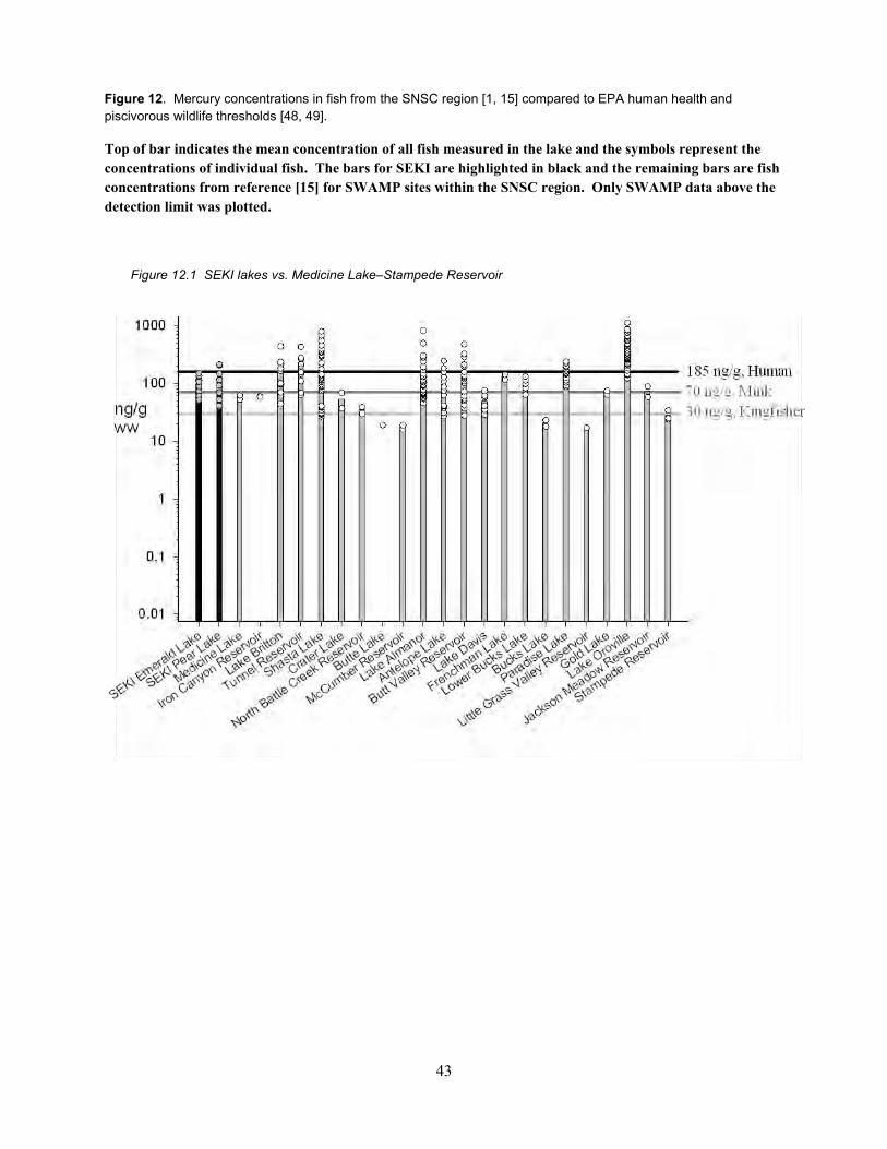
43

Figure 12. Mercury concentrations in fish from the SNSC region [1, 15] compared to EPA human health and piscivorous wildlife thresholds [48, 49].

Top of bar indicates the mean concentration of all fish measured in the lake and the symbols represent the concentrations of individual fish. The bars for SEKI are highlighted in black and the remaining bars are fish concentrations from reference [15] for SWAMP sites within the SNSC region. Only SWAMP data above the detection limit was plotted.

Figure 12.1 SEKI lakes vs. Medicine Lake–Stampede Reservoir

44

Figure 12.2 SEKI lakes vs. Bowman Lake–Lake Combie

Figure 12.3 SEKI lakes vs. Loon Lake–Pinecrest

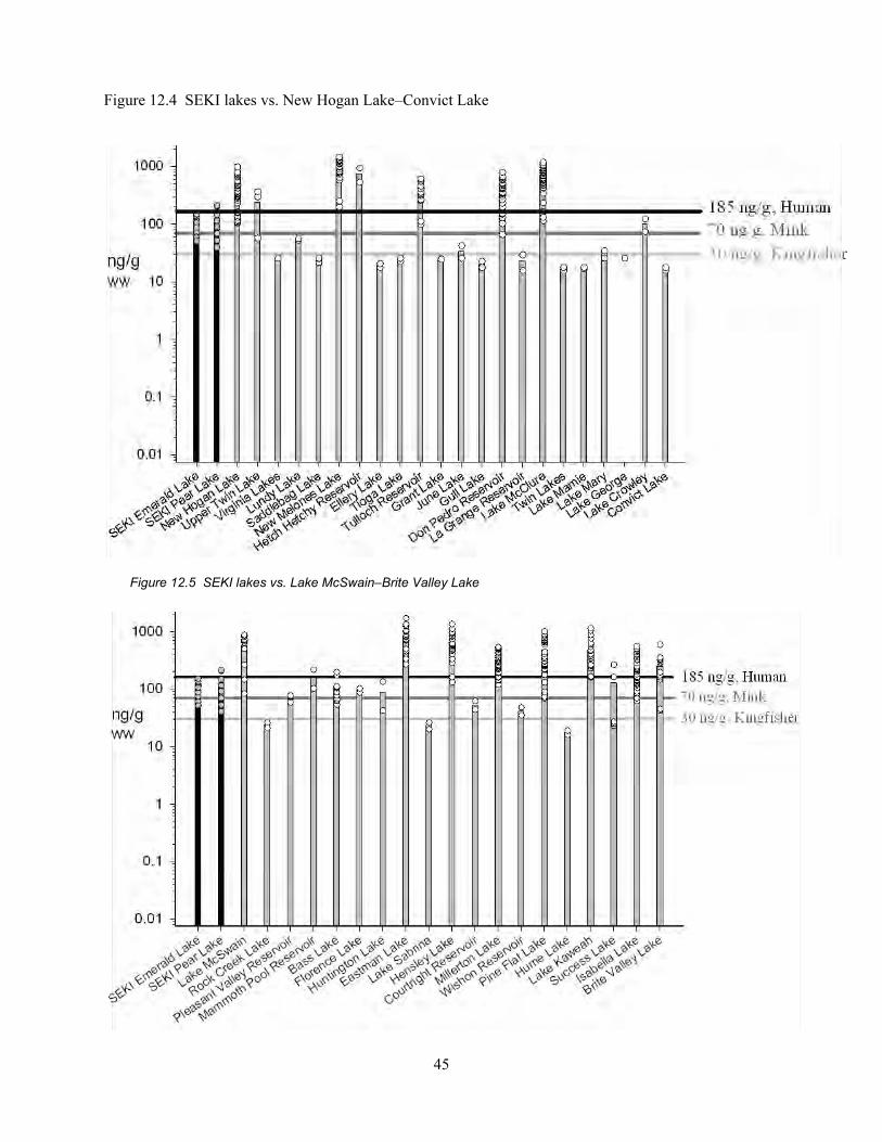
45

Figure 12.4 SEKI lakes vs. New Hogan Lake–Convict Lake

Figure 12.5 SEKI lakes vs. Lake McSwain–Brite Valley Lake

46

Table 5. Recent mercury health thresholds for humans and piscivorous wildlife and percent of SNSC fish [1, 15] that exceed the threshold.

Species Mercury Concentration in Fish–wet wt

% of SNSC Fish Exceeding Threshold Source of Health Threshold

Humans 300 ng/g fillet, 185 ng/g whole 56 EPA[64]

Piscivorous Wildlife 270 ng/g fillet, 150 ng/g whole 62 EPA[64]

Piscivorous Fish ~500 ng/g muscle, 200 ng/g whole 54 Beckvar et al.[65], Dillon et al. [66],

Sandheinrich et al.[67]

Piscivorous Wildlife—Otter 100 ng/g whole 74 Lazorchak et al.[49]

Piscivorous Wildlife—Mink 70 ng/g whole 81 Lazorchak et al.[49], Walters et al.

[68]

Piscivorous Wildlife—Belted Kingfisher

30 ng/g whole 92 Lazorchak et al.[49], Walters et al. [68]

47

2.6. Emerging Contaminants Emerging contaminants of interest in the SNSC region include polybrominated diphenyl ether (PBDE) flame retardants, as well as perfluorinated compounds (PFCs). These compounds are used in a wide variety of consumer products (including fabrics and electronics) and their emissions tend to be highest in urban areas.

Relatively few measurements have been made on these compounds in the SNSC region and the measurements that have been made were in SEKI (fish and sediment) and YOSE [1, 27]. PBDEs were measured in fish and dated sediment cores collected from Emerald and Pear Lakes in SEKI as part of WACAP [1]. PBDEs were measured in YOSE but the concentrations in blank samples were similar to the concentrations in actual samples and the data were not interpreted [27]. PBDEs were not measured in fish collected by SWAMP. The PBDE concentrations in SEKI fish were comparable to other WACAP parks and did not exceed human health thresholds [1, 13]. Wildlife contaminant health thresholds have not been established for PBDEs. PBDEs were detected in the Emerald Lake sediment core but not in the Pear Lake sediment core and no temporal trend was obvious [1]. PFCs are not known to have been measured in SNSC ecosystems.

Because of recent U.S. legislation to phase-out and/or restrict the use of some PBDEs and PFCs, their deposition to SNSC ecosystems is expected to remain constant and/or decline in the future. However, it is possible that new chemical replacements in consumer products may also undergo deposition to SNSC ecosystems.

Recommendations: PBDEs (and likely PFCs) undergo deposition to SNSC ecosystems from use in urban areas of California. Limited data indicate that the PBDE concentrations in SNSC fish do not currently exceed human health thresholds. Unless health thresholds for these chemicals change, it is recommended that SNSC researchers stay informed of the literature on deposition of other emerging pollutants to remote ecosystems (including the Arctic) instead of making additional measurements of PBDEs (and PFCs) in SNSC ecosystems. This could be done by contracting a literature review of emerging pesticides of concern and evaluating the risk to SNSC ecosystems on a 5–10 year cycle.

Potential Outcome: If changes in the deposition of emerging pollutants are observed in other remote ecosystems (such as the Arctic) new studies on emerging pollutants can be established in the SNSC region.

48

3. Ecosystem Indicators Used for Measuring Air Toxics in the SNSC Region The different ecosystem indicators (different environmental media) used in SNSC studies to study air toxics, air toxics measured by these indicators, as well as their advantages and disadvantages are summarized in Figure 6.

3.1. Atmospheric Ideally, active air sampling would be used to quantitatively measure air toxics in the SNSC region atmosphere with high spatial and temporal resolution. However, significant challenges presented with mountainous terrain and the limited availability of electricity to run active air samplers have prevented this except in locations near buildings with electricity, such as at the IMPROVE (Interagency Monitoring of Protected Visual Environments) sites (http://vista.cira.colostate.edu/improve/). To increase the spatial resolution of air toxics measurements in the SNSC region, scientists have used passive air sampling devices (PASDs), lichen, conifer needles, snow, and rain to measure air toxics in the SNSC region (Table 6).

As part of WACAP, CUPs, HUPs, PCBs, and PAHs were measured in lichen, conifer needles, snowpack, and XAD-based PASDs collected from 19 different U.S. national parks (including SEKI, YOSE, and LAVO) in order to compare the magnitude and mechanism of air toxics accumulation in the different passive sampling media [69]. Lichen accumulated the highest concentrations, in part because of its long (and unknown) exposure period, while PASDs accumulated the lowest concentrations. However, only the PASD concentrations can be used to calculate an average atmospheric gas-phase concentration because the sampling rates are known and the media is uniform. Of the passive air sampling media measured, only lichen and snowpack accumulation profiles were found to be statistically significantly correlated with each other because they both accumulate air toxics present in the atmospheric particle-phase. This suggests that needles and PASDs represent a different composition of the atmosphere than lichen and snowpack and that the interpretation of which air toxics are present is dependent on the type of passive sampling media used. All four passive sampling media preferentially accumulated compounds with relatively low air-water partition coefficients, while snowpack accumulated compounds with higher log octanol-air partition coefficients compared to the other media. Lichen showed a greater accumulation of particle-phase PAHs relative to needles.

The proper selection of passive air sampling media for measuring CUPs, HUPs, PCBs, PAHs, and mercury is dependent on the study design; including

the geographic location of the study (presence of vegetation, ambient temperature, and ease of access),

the air toxics of interest (vapor pressure and whether the air toxic is present in the gas or particle phases), and

the exposure time period of interest (season, as well as the duration and accuracy of knowing the exposure time period) [69].

If average concentrations of gas-phase air toxics in air are needed, then PASDs should be used because their sampling rates are known for many air toxics. Precipitation, especially snow, is an important route of deposition of air toxics to SNSC ecosystems. Therefore, annual snowpack is a useful indicator of

http://vista.cira.colostate.edu/improve/

49

which air toxics are entering SNSC ecosystems, especially during the spring snowmelt. Conifer needles and lichens are useful for comparing the relative concentrations of air toxics among different sites and are relatively easy to collect. However, they cannot be used to determine the actual concentrations in air because their sampling rates (and age of lichen) are not known.

As part of WACAP, mercury was measured in annual snowpack, conifer needles, and lichen in SEKI [1] and mercury has been measured in snow collected from the Sagehen basin in the central Sierra Nevada [60]. In addition, a National Atmospheric Deposition Program (NADP)–Mercury Deposition Network (MDN) site currently exists at SEKI to measure mercury in wet precipitation (http://nadp.sws.uiuc.edu/mdn/) [59]. Atmospheric mercury speciation is also being measured at YOSE as part of a study seeking to identify potential sources of airborne mercury and its deposition through California and Nevada.

Recommendation: Although wet deposition of air toxics through rainfall occurs, it is recommended that annual snowpack be used to determine the annual input of air toxics to SNSC ecosystems because it is an important route of atmospheric deposition and scavenges a wide array of air toxics from the atmosphere (both gas-phase and particle-phase and mercury as well as organic air toxics). It is also likely the major route of deposition for SNSC cold, high elevation ecosystems [27]. However, annual snowpack is more difficult to collect than some of the other passive sampling media and does not provide an actual measure of concentration in the atmosphere. Passive air samplers are being developed for mercury and may be of use in the SNSC region for the validation of future mercury deposition models. The proper selection of passive air sampling media is ultimately dependent on the study design as outlined above.

Potential Outcome: Measurement of air toxics in annual snowpack, and associated atmospheric modeling, will provide temporal information on which air toxics are being deposited to SNSC ecosystems and how deposition is changing over time.

3.2. Aquatic Surface water (generally lake water), sediment cores, and surficial sediment have been used as abiotic indicators to determine which air toxics are accumulating in SNSC aquatic ecosystems (Table 6). These abiotic indicators are useful because they provide information on what aquatic organisms are exposed to via the aquatic ecosystem. In general, sediments have much higher concentrations of air toxics than surface water because most hydrophobic organic air toxics (and methylmercury) preferentially accumulate in sediment rather than in water. In addition, dated sediment cores can provide useful information on the temporal deposition of air toxics to aquatic ecosystems but are challenging to collect from deep lakes.

Fish and amphibians have been frequently used in the SNSC region as biotic indicators to determine the bioaccumulation, biomagnification, and potential health effects of air toxics in SNSC aquatic ecosystems (Table 6). Fish generally have higher concentrations of air toxics (and methylmercury) than amphibians because fish have higher lipid concentrations. Some species of fish also represent the top of the aquatic food web and are consumed by humans and/or piscivorous wildlife, presenting an important trophic link to human and wildlife health. Regardless, amphibians and other aquatic organisms are sensitive to air toxics and warrant further study and protection, especially those species that have undergone population

http://nadp.sws.uiuc.edu/mdn/

50

declines. Only one study has looked at the accumulation of mercury in a piscivorous bird species, Western Grebes, collected from the SNSC region [70]. Other piscivorous birds including eagles, osprey, and the common loon have been utilized in studies from regions outside the SNSC. Moreover, aquatic invertebrate like the dragonfly larvae (Odonata: anisoptera) are being explored as sentinel species for mercury contamination, including in national parks.

Recommendation (1): In view of the preferential accumulation of air toxics (and methylmercury) in sediments and fish, as compared to water, and the relevance of fish to human and piscivorous wildlife health, fish are good ecosystem indicators to measure in SNSC aquatic ecosystems. Given that some SNSC fish currently exceed human and wildlife consumption thresholds for some air toxics (mercury, dieldrin, DDTs, chlordanes, and PCBs), it is especially important to understand (and be able to predict) the spatial distribution of these exceedances. Dragonfly larvae and piscivorous bird species may also be used as an indicator for mercury in aquatic ecosystems.

Recommendation (2): Unfortunately, it is not currently possible to predict the spatial variation in air toxics bioaccumulation in aquatic ecosystems within the SNSC region and additional research is needed in this area. Examples of this type of research are the dragonfly larvae studies and mercury ecosystem models being developed for national parks (and the SNSC region) by the USGS.

Potential Outcome: Understanding the spatial variation of air toxics bioaccumulation in SNSC aquatic food webs may allow for the prediction of which lakes will contain fish that exceed human and piscivorous wildlife consumption thresholds. Resource managers could use these predictions to conduct more comprehensive sampling of biotic resources in these selected areas.

3.3. Terrestrial Conifer needles and lichen have not only been used as indicators for measuring air toxics in the atmosphere, but they are also indicators for measuring air toxics in the terrestrial ecosystem because they are a part of the terrestrial ecosystem and are eventually incorporated into SNSC region soils [1] (Table 6).

It should be noted that, to date, soils have not been used to study the spatial distribution of CUPs, HUPs, PCBs, and mercury in SNSC terrestrial ecosystems. However, soils are high in organic matter that binds these air toxics and accumulates air toxics over decades from decaying vegetation (resulting in higher air toxics concentrations than the vegetation itself) [1]. Soils are also relatively easy to collect. Mercury was measured in soils collected from the Sagehen basin in the central Sierra Nevada [60]. To date, the accumulation of mercury in insectivorous bird species has not been studied in the SNSC region, yet an assessment of mercury in songbirds at YOSE and other western national parks is underway. Similar studies on songbirds in the Northeastern U.S. suggest that these bird groups are important indicators for mercury in terrestrial ecosystems [95].

Recommendations: Predicting the spatial variation in air toxics bioaccumulation in terrestrial ecosystems within the SNSC region is not currently possible and additional research is needed in this area. If concerns about the loading and flux of air toxics to SNSC terrestrial ecosystems arise, soils may be useful as an indicator for measuring air toxics in terrestrial ecosystems, especially for CUPs, HUPs, PCBs, and mercury. Insectivorous songbirds may also be used as an indicator for mercury in terrestrial ecosystems.

51

Potential Outcome: Understanding the spatial distribution of air toxics in SNSC terrestrial ecosystems will allow prediction of which terrestrial ecosystems will have the highest air toxics concentrations.

52

Table 6. Ecosystem indicators previously used for air toxics monitoring in the SNSC region.

Ecosystem Indicator Which Air Toxics Can Be Measured? Advantages Disadvantages

Air

(Active and Passive Air Sampling Devices)[1, 8, 24, 26, 29, 69, 71–74]

Pesticides Passive-gas Phase

PAHs only Active–gas and

particle phase PAHs PCBs Mercury

Uniformly made Can calculate atmospheric

concentration directly Active–accumulates episodic

(24 hr) transport Passive–accumulation over 1

to 12 month deployment periods

2 trips/sample–deploy and collect

Passive-low concentrations and samples only gas phase pollutants

Active–requires electricity

Vegetation

(Lichen and Conifer Needles)[1, 24, 27, 55, 69]

Pesticides All PAHs PCBs Mercury

Part of terrestrial ecosystem Conifer needles may be

dated High concentrations Accumulation over organism

life-span

Cannot directly calculate an atmospheric concentration

Difficult to measure in matrix

Species differences in accumulation

Snow

[1, 5, 6, 27–29, 45, 51, 55, 59, 60, 69]


Net deposition to ecosystem Major route of deposition in

Fall/Winter/Spring Accumulation over snow

accumulation period

Low concentrations Large volumes (50L)

needed for low detection limits

Rain

[27–29, 59]


Net deposition to ecosystem Major route of deposition in

Summer

Episodic so difficult to collect

Large volumes (20L) needed

Surface Water

[1, 25–27, 51, 60, 75]


CUPs present in summer Exposure route to aquatic

organisms

Very low concentrations

Large volumes needed (>50L or long SPMD exposure periods) for low detection limits

Accumulation over residence time of lake

Lake Sediment Cores

[1, 55–58]

Pesticides All PAHs PCBs PBDE flame

retardants Mercury

Historical and present day deposition comparison possible

Higher concentrations

Difficult to collect Must be dated

Surficial Lake Sediment

[1, 8, 27, 45, 55, 75]


Easy to collect Exposure route to aquatic

organisms Higher concentrations

Mix of historical and present deposition (no dating)

53

Ecosystem Indicator Which Air Toxics Can Be Measured? Advantages Disadvantages

Fish

[1, 4, 13–15, 33, 35, 45, 50, 51, 76, 77]

Pesticides All PAHs PCBs PBDE flame

retardants Mercury

Part of aquatic ecosystem Higher concentrations Fish consumption advisories

for HUPs, some CUPs and Mercury

Standard methods and more routine measurement

Accumulation over organism life-span

Variability in bioaccumulation due to species and ecosystem differences

Amphibians

[7–11, 16, 17, 33, 34, 46, 61, 78]


Part of terrestrial and aquatic ecosystems

Some species are endangered/threatened


Low concentrations Variability in

bioaccumulation due to species and ecosystem differences

Species/stage that is common and easy to sample is short lived

Birds

[70] Mercury

Part of terrestrial and/or aquatic ecosystem

Blood is relatively easy to collect and can be measured for Mercury [79]


Potential for migration and exposure in different geographic locations

Variability in bioaccumulation due to species and ecosystem differences

Reference numbers for relevant literature are given in brackets.

54

4. Spatial Distribution of Air Toxics in Different Ecosystem Indicators The spatial extent of sites sampled over the past two decades (1990–2009) with available data on air toxics in fish, surface water, vegetation, snow, air, sediments, and amphibians in the SNSC region are shown in Figure 13. The ecosystem indicator with the greatest spatial coverage across the SNSC study area is fish, followed by surface water and vegetation (Figure 13). Multiple air toxics studies conducted in YOSE, SEKI, and LAVO from 1990–2009 included additional ecosystem indicators and represent widespread spatial distribution within NPS boundaries (Figures 14.1, 14.2, and 14.3). When all ecosystem indicators are combined there is widespread spatial coverage of air toxics data in the SNSC region (Figure 13), particularly for FS and NPS lands. To further assess the spatial distribution of available air toxics data in the SNSC region, maps have been developed for each individual ecosystem indicator. These maps were created by compiling available air toxics data from previous studies, summarized spatially and temporally in the annotated bibliography (Figures 13, 14; Appendix D). Additionally, concentration maps have been developed for available data on dominant CUPs (endosulfan, chlorpyrifos, dacthal), HUPs (dieldrin), mercury, and PCBs for each ecosystem indicator and are discussed in the following sections.

The spatial distribution of air toxics in the SNSC region is dependent upon: 1) variation in atmospheric concentrations and deposition, and 2) variation in air toxics accumulation in ecosystems. In order to evaluate the spatial variation in air toxics atmospheric concentrations and deposition, ecosystem indicators that are directly linked to the atmosphere, such as air and precipitation, should be used. In order to evaluate the spatial variation in the combined effects of variation in air toxics atmospheric concentrations and deposition and accumulation in aquatic and terrestrial ecosystems, ecosystem indicators such as annual snowpack, biota, sediments, and soils should be used. Annual snowpack is affected by aging processes (including volatilization and chemical reactions) over time so that the spatial variation in air toxics concentrations or fluxes in snowpack may be a function of both atmospheric deposition and the ecosystem (including shade and topography). Other significant within ecosystem factors that can influence the spatial distribution of air toxics include species differences, trophic differences, and differences in organic matter content. However, when evaluating the spatial distribution of air toxics, it is best to compare the same ecosystem indicator (including species if applicable), collected at the same time at different sites, and air toxics measurements made, preferably, in the same laboratory. This will help to minimize variation due to species, temporal, and laboratory differences.

A comparison of CUP, HUP, PCB, and PAH concentrations in tadpole and surficial sediment measured in the same laboratory and collected across the Lassen and Klamath regions (Pseudacris regilla) [34], Yosemite National Park (Pseudacris sierra) [80], and Sequoia and Kings Canyon National Parks (Pseudacris sierra) [7] sheds light on the spatial distribution of air toxics in tadpoles and surficial sediments from north to south within the SNSC region. In general, the concentrations of CUPs and HUPs appear to increase from north to south within the SNSC region, with the highest concentrations in Sequoia and Kings Canyon National Parks. A similar north to south spatial trend within the Sierra Nevada Mountains was identified for DDE in frogs in 1970 [46]. The PAH concentrations appear to be highest in the central SNSC region, with the highest concentrations in Yosemite National Park, while the PCB concentrations do not appear to show a spatial trend. However, a more detailed analysis of these data and

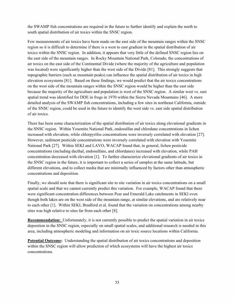
55

the SWAMP fish concentrations are required in the future to further identify and explain the north to south spatial distribution of air toxics within the SNSC region.

Few measurements of air toxics have been made on the east side of the mountain ranges within the SNSC region so it is difficult to determine if there is a west to east gradient in the spatial distribution of air toxics within the SNSC region. In addition, it appears that very little of the defined SNSC region lies on the east side of the mountain ranges. In Rocky Mountain National Park, Colorado, the concentrations of air toxics on the east side of the Continental Divide (where the majority of the agriculture and population was located) were significantly higher than the west side of the Divide [81]. This strongly suggests that topographic barriers (such as mountain peaks) can influence the spatial distribution of air toxics in high elevation ecosystems [81]. Based on these findings, we would predict that the air toxics concentrations on the west side of the mountain ranges within the SNSC region would be higher than the east side because the majority of the agriculture and population is west of the SNSC region. A similar west vs. east spatial trend was identified for DDE in frogs in 1970 within the Sierra Nevada Mountains [46]. A more detailed analysis of the SWAMP fish concentrations, including a few sites in northeast California, outside of the SNSC region, could be used in the future to identify the west side vs. east side spatial distribution of air toxics.

There has been some characterization of the spatial distribution of air toxics along elevational gradients in the SNSC region. Within Yosemite National Park, endosulfan and chlordane concentrations in lichen increased with elevation, while chlorpyrifos concentrations were inversely correlated with elevation [27]. However, sediment pesticide concentrations were inversely correlated with elevation with Yosemite National Park [27]. Within SEKI and LAVO, WACAP found that, in general, lichen pesticide concentrations (including dacthal, endosulfans, and chlordanes) increased with elevation, while PAH concentration decreased with elevation [1]. To further characterize elevational gradients of air toxics in the SNSC region in the future, it is important to collect a series of samples at the same latitude, but different elevations, and to collect media that are minimally influenced by factors other than atmospheric concentrations and deposition.

Finally, we should note that there is significant site to site variation in air toxics concentrations on a small spatial scale and that we cannot currently predict this variation. For example, WACAP found that there were significant concentration differences between Pear and Emerald Lake catchments in SEKI even though both lakes are on the west side of the mountain range, at similar elevations, and are relatively near to each other [1]. Within SEKI, Bradford et al. found that the variation on concentrations among nearby sites was high relative to sites far from each other [8].

Recommendation: Unfortunately, it is not currently possible to predict the spatial variation in air toxics deposition in the SNSC region, especially on small spatial scales, and additional research is needed in this area, including atmospheric modeling and information on air toxic source locations within California.

Potential Outcome: Understanding the spatial distribution of air toxics concentrations and deposition within the SNSC region will allow prediction of which ecosystems will have the highest air toxics concentrations.

56

Figure 13. Sampling locations and sample type for toxic air contaminants in the SNSC region (1990–2009).

References: [1, 4–8, 10, 13, 16, 17, 24–27, 29, 33–35, 50, 60, 75, 76, Appendix D]

57

Figure 14. Sampling locations and sample type for toxic air contaminants at national parks in the SNSC region (1990–2009).

Figure 14.1 Yosemite National Park.

References: [1, 16, 27, 35, 75, Appendix D]

58

Figure 14.3 Sequoia and Kings Canyon National Parks.

References: [1, 6, 8, 16, 17, 25, 26, 29, 50, Appendix D]

59

Figure 14.4 Lassen Volcanic National Park.

References: [1, 34, 35, 75, Appendix D]

60

4.1. Fish Air toxics sampling in fish has fairly even spatial distribution throughout the SNSC region. Fish sampling from SWAMP, studies within the National Parks, and data compiled from relevant literature contribute to this picture of sampling in the region (Figure 15) [1, 35, 50, 75, Appendix D].

Mercury was detected in all fish sampled in the SNSC region from 2001–2009, ranging in concentration from 0.1–2 µg ww (Figure 16) [1, 75, Appendix D]. Higher mercury concentrations were detected at lower elevations outside National Park boundaries [75].

PCBs, ranging from 0–56 ng/g ww, were detected within National Park boundaries and also in the surrounding area (Figure 17) [1, 35, 50, 75]. There is no clear spatial pattern for PCBs detected in SNSC fish.

Chlorpyrifos was detected in fish at higher elevations within NPS boundaries (Figure 18) [1, 35]. However, few fish samples were analyzed for chlorpyrifos as part of SWAMP [75], which limits the spatial extent of available data. Dieldrin and endosulfan showed variable spatial patterns. Dieldrin was detected in many fish sampled in the SNSC region including fish from high-elevation sites in LAVO, YOSE, and SEKI (Figure 19) [1, 35, 75]. However, only 3 sites had dieldrin concentrations in fish greater than 1 ng/g ww. The highest concentration of dieldrin in fish (>10 ng/g ww) was found in SEKI [1, 35, 75]. Endosulfan was detected in fish from LAVO, YOSE, and SEKI but was not detected outside of NPS boundaries (Figure 20) [1, 35, 75]. Dacthal was also detected in fish in LAVO, YOSE, and SEKI (Figure 21) [1, 35, 75].

Fish collected from the SNSC region do not exceed EPA health guidelines or OEHHA human health FCGs for chlordanes, DDTs, or PCBs (Tables 2 and 3; Section 2.2). However, approximately 6 % of SNSC fish measured by SWAMP and WACAP exceed the threshold value of OEHHA FCGs for dieldrin and mercury (Table 2; Section 2.2). Future studies are expected to improve the spatial distribution of data on CUPs, HUPs, PCBs, and mercury in fish in LAVO, YOSE, and SEKI, and continue to measure air toxics in fish throughout the SNSC region.

61

Figure 15. Fish sampling sites in the SNSC region (2001–2009).

References: [1, 35, 50, 75]

62

Figure 16. Total mercury concentrations in fish (2001–2009).

References: [1, 75]

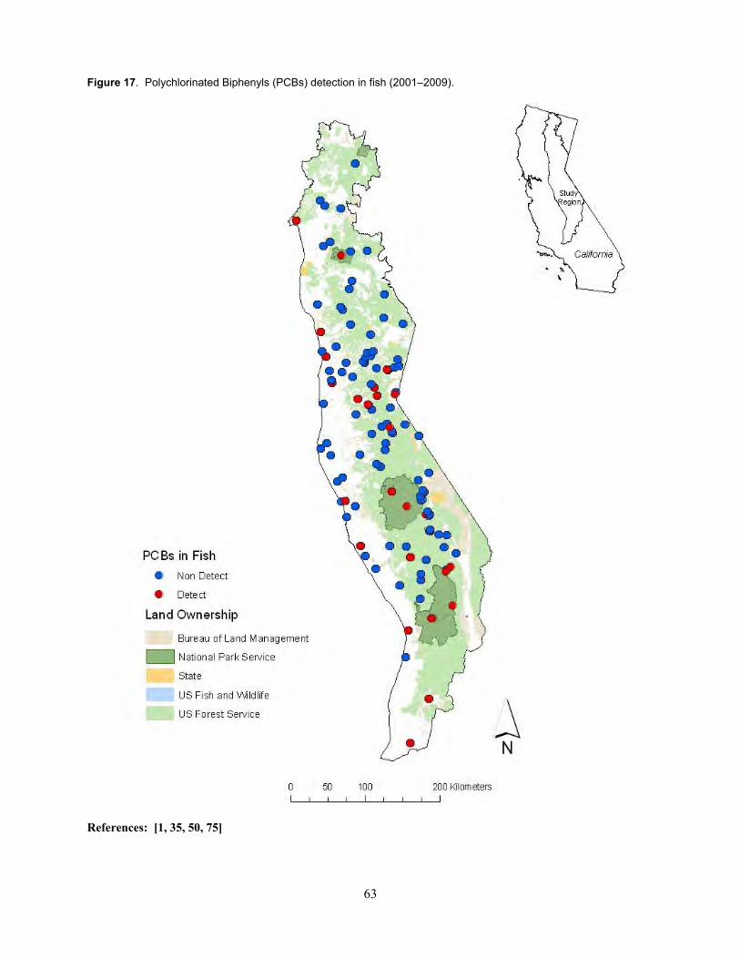
63

Figure 17. Polychlorinated Biphenyls (PCBs) detection in fish (2001–2009).

References: [1, 35, 50, 75]

64

Figure 18. Chlorpyrifos detection in fish (2001–2009).

References: [1, 35, 75]

65

Figure 19. Dieldrin concentrations in fish (2001–2009).


66

Figure 20. Endosulfan detection in fish (2001–2009).


67

Figure 21. Dacthal detection in fish (2001–2009).


68

4.2. Surface Water The majority of surface water sites with available air toxics data in the SNSC region (1997–2009) are located in LAVO, SEKI, and YOSE [Figure 22] [1, 25–27, Appendix D]. Surface water data for CUPs, HUPs, PCBs, and mercury are available for YOSE, SEKI, and outside the SEKI boundary in the southern Sierra Mountains, but not in LAVO [1, 25-27, 51, 60, 75].

In general, the highest concentrations of air toxics and most frequent detections are in SEKI, followed by YOSE and LAVO. (LAVO, however, only has available data for mercury concentrations in surface water.) Endosulfan was detected in all surface waters with available air toxics data in SEKI and YOSE with concentrations ranging from detection to 24.8 ng/L (Figure 23) [1, 25–27]. The high endosulfan concentrations (>1 ng/L) are along an elevational transect in SEKI that extends beyond the NPS boundary (Figure 23). In general, endosulfan concentrations increase with decreasing elevation [1, 25–27]. Chlorpyrifos was not detected in YOSE surface water and was detected in SEKI (Figure 24) [1, 25–27], with a maximum concentration > 100 ng/L. Sites with relatively high concentrations of chlorpyrifos in surface water were collected in 1997 [27]. Dieldrin was detected in SEKI and at two sites in YOSE (Figure 25) [1, 27]. Dacthal was detected in all surface water samples in both YOSE and SEKI and ranged in concentration from 0.02 ng/L to 0.52 ng/L (Figure 26) [1, 27]. Total mercury concentrations were highest in SEKI, with a maximum concentration of 3.0 ng/L (Figure 27) [1, Appendix D]. PCBs were not detected in surface waters in YOSE, but low levels were detected at Emerald Lake (0.4 ng/L) and Pear Lake (0.4 ng/L) in SEKI (Figure 28) [1, 27]. To increase the spatial distribution of data on air toxics in SNSC surface waters, it is recommended that future studies include areas that extend beyond NPS boundaries in the southern Sierra Mountains where detections of air toxics are more frequent and concentrations are higher. However, because of low concentrations due to low water solubility and temporal variability, as well as high detection limits, measuring air toxics including CUPs, HUPs, and PCBs in SNSC surface waters is not a priority.

69

Figure 22. Surface water sampling sites (1997–2009).

References: [1, 25–27]

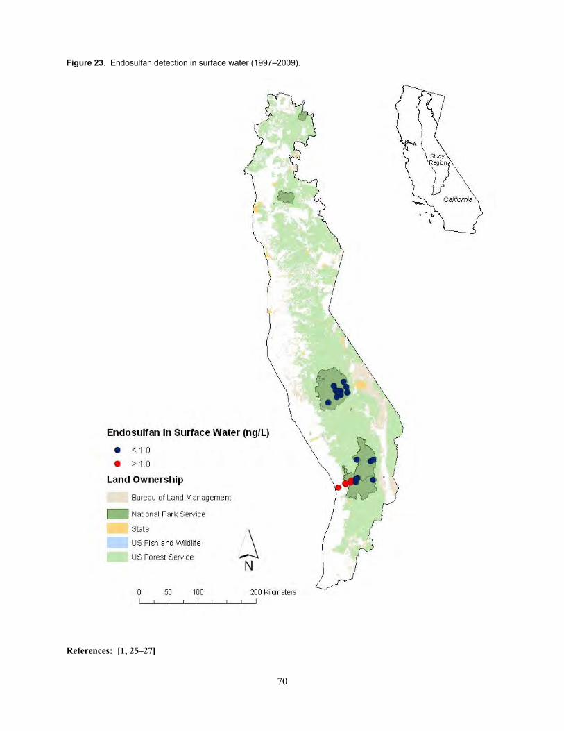
70

Figure 23. Endosulfan detection in surface water (1997–2009).


71

Figure 24. Chlorpyrifos concentration in surface water (1997–2009).


72

Figure 25. Dieldrin detection in surface water (2002–2009).

References: [1, 27]

73

Figure 26. Dacthal detection in surface water (2002–2009).

References: [1, 27]

74

Figure 27. Total mercury concentrations in surface water (1999–2009).

References: [1, Appendix D]

75

Figure 28. Polychlorinated Biphenyls (PCBs) detection in surface water (2002–2009).

References: [1, 27]

76

4.3. Snow In the SNSC region, available data on air toxics in snow from 2002–2009 includes NPS sites in SEKI and YOSE, and a non-NPS site at Sagehen in the central Sierra Nevada (Figure 29) [1, 5, 6, 27, Appendix D]. Endosulfan, chlorpyrifos, dacthal, dieldrin, and mercury were detected in snow at high-elevation sites in SEKI and YOSE (Figures 29–35). In general, the difference in chemical concentrations in snow between YOSE and SEKI was low [1, 5, 6, 27]. Endosulfan and chlorpyrifos yielded higher concentrations in snow in YOSE than SEKI with concentrations ranging from detection to over 3 ng/L (Figures 30 and 32) [1, 5, 6, 27]. Dieldrin concentrations in snow ranged from detection to 2 ng/L, with higher concentrations detected in SEKI (Figure 31) [1, 5, 6, 27]. Dacthal concentrations in snow ranged from detection to over 3 ng/L with high concentrations in both SEKI and YOSE (Figure 33) [1, 5, 6, 27]. Mercury concentrations in snow ranged from detection to over 1.5 ng/L with the highest concentrations at Sagehen and levels up to 1.5 ng/L in YOSE and SEKI (Figure 34) [1, 5, 6, 27]. PCBs were not detected in snow in the SNSC region (Figure 35) [1, 27].

More sampling sites are needed to model toxic air contaminant deposition for the SNSC region using chemical concentrations in snow. This is due to limited data available on pesticides and mercury in snowpack, and poor spatial distribution of sites across the SNSC region, particularly for areas that extend beyond YOSE and SEKI boundaries. It may be possible to model toxic air contaminant deposition in snow for a smaller area such as YOSE.

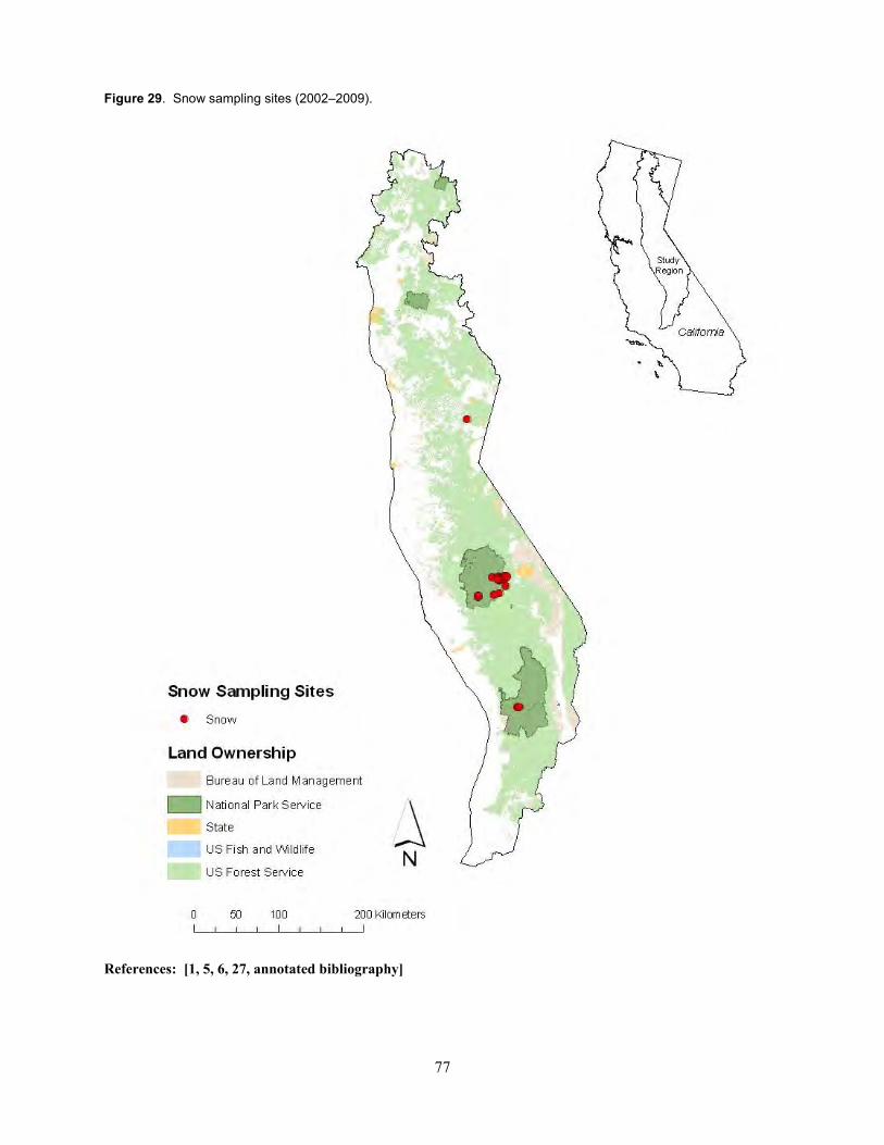
77

Figure 29. Snow sampling sites (2002–2009).

References: [1, 5, 6, 27, annotated bibliography]

78

Figure 30. Endosulfan concentrations in snow (2002–2009).

References: [1, 5, 6, 27]

79

Figure 31. Dieldrin concentrations in snow (2002–2009).


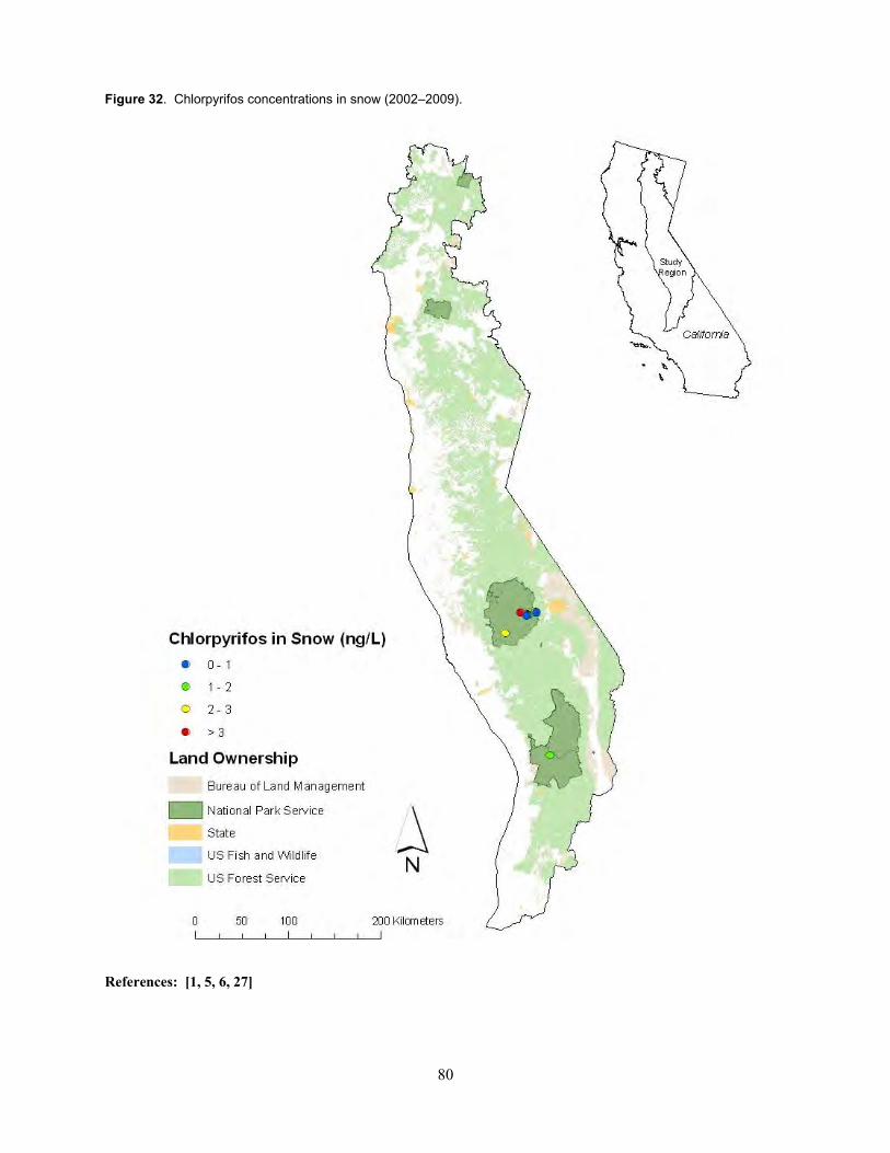
80

Figure 32. Chlorpyrifos concentrations in snow (2002–2009).


81

Figure 33. Dacthal concentrations in snow (2002–2009).


82

Figure 34. Total mercury concentrations in snow (2002–2009).

References: [1, Appendix D]

83

Figure 35. Polychlorinated Biphenyls (PCBs) detection in snow (2002–2009).


84

4.4. Vegetation The spatial distribution of air toxics sampled in vegetation in the SNSC region is shown in Figure 36 [1, 27, Appendix D]. Available data on air toxics in vegetation (i.e., lichen, conifer needles) in the SNSC region include sites in SEKI, YOSE, and LAVO (Figure 36), with no sites outside NPS boundaries.

For the following figures (37–41), vegetation includes both lichen and conifer needles and is indicated as detect if at least one type of vegetation has an air toxic detected [1, 27]. Endosulfan detections in vegetation in the SNSC region are shown in Figure 37 [1, 27]. All vegetation sampled in SEKI, YOSE, and LAVO had detections for endosulfan, with the exception of one conifer needle sample in SEKI [1]. The same conifer needle sample also had no detect for chlorpyrifos, dieldrin, and dacthal [1]. Chlorpyrifos was detected in vegetation at all sites in SEKI and LAVO, and the majority of sites in YOSE (Figure 38) [1, 27]. Dieldrin was also detected in vegetation in SEKI, LAVO, and sites in YOSE (Figure 39) [1, 27]. Dacthal was detected at all vegetation sites in SNSC (Figure 40) [1, 27]. PCBs were detected in SEKI and LAVO, but PCBs were not detected in vegetation for many sites in YOSE (Figure 41) [1, 27]. The spatial extent of data on mercury in vegetation in the SNSC region is limited, though vegetation may not be the best indicator for deposition or bioaccumulation of mercury (written commun., Tarnay). However, mercury was detected in lichen in SEKI [1]. To increase the spatial distribution of air toxics data in the SNSC region in the terrestrial ecosystem, it is recommended that vegetation be collected in areas that extend beyond YOSE, SEKI, and LAVO.

85

Figure 36. Vegetation sampling sites (2002–2009).

References: [1, 27, Appendix D]. Note: Vegetation includes lichen and conifer needles.

86

Figure 37. Endosulfan detection in vegetation (2002–2009).

References: [1, 27]. Note: Vegetation includes lichen and conifer needles.

87

Figure 38. Chlorpyrifos detection in vegetation (2002–2009).


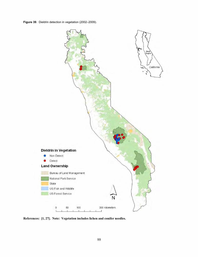
88

Figure 39. Dieldrin detection in vegetation (2002–2009).


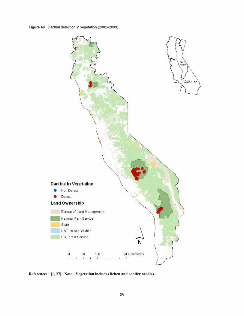
89

Figure 40. Dacthal detection in vegetation (2002–2009).


90

Figure 41. Polychlorinated Biphenyls (PCBs) detection in vegetation (2002–2009).


91

4.5. Air and Sediment Air toxics sampled in air in the SNSC region were collected from active and passive air monitors located in YOSE, LAVO, SEKI, and in the southern Sierra Mountains from 1990–2009 [1, 8, 26, 29] (Figure 42). Dry deposition monitoring sites are also included in Figure 42 as data representing the portion of atmospheric deposition that settles as dust or deposits on surfaces (e.g., vegetation, snow) during periods of no precipitation. Available data on air toxics in surface sediment and lake sediment cores [1, 8, 27, 34] are shown in Figure 43. Spatially distributed air toxics data from air and sediment samples were reported during a 2005 study at 28 SEKI site locations shown in Figures 42 and 43 [8]. CUPs, HUPs, and PCBs were detected frequently at low concentrations in sediment in 2005 in SEKI, and endosulfan was detected in air [8]. In WACAP, low level concentrations of endosulfan, PCBs, and dacthal were detected in air in LAVO, SEKI, and YOSE [1].

Recent work on air toxics in surface sediment sampled in 2008 and 2009 in YOSE found low concentrations to non-detects at sites shown in Figure 43 [27], however there was an inverse correlation with elevation. The spatial extent of available data on air toxics in air and surface sediment is limited in the SNSC region and could be expanded to gain a better understanding of current and future conditions.

92

Figure 42. Air and dry deposition sampling sites (1990–2009).

References: [1, 8, 26, 29].

93

Figure 43. Sediment sampling sites (2002–2009).

References: [1, 8, 27, 34]

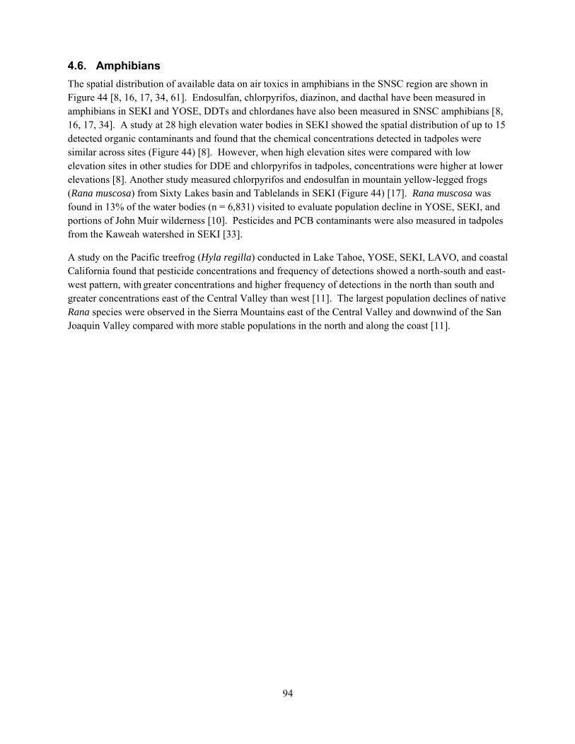
94

4.6. Amphibians The spatial distribution of available data on air toxics in amphibians in the SNSC region are shown in Figure 44 [8, 16, 17, 34, 61]. Endosulfan, chlorpyrifos, diazinon, and dacthal have been measured in amphibians in SEKI and YOSE, DDTs and chlordanes have also been measured in SNSC amphibians [8, 16, 17, 34]. A study at 28 high elevation water bodies in SEKI showed the spatial distribution of up to 15 detected organic contaminants and found that the chemical concentrations detected in tadpoles were similar across sites (Figure 44) [8]. However, when high elevation sites were compared with low elevation sites in other studies for DDE and chlorpyrifos in tadpoles, concentrations were higher at lower elevations [8]. Another study measured chlorpyrifos and endosulfan in mountain yellow-legged frogs (Rana muscosa) from Sixty Lakes basin and Tablelands in SEKI (Figure 44) [17]. Rana muscosa was found in 13% of the water bodies (n = 6,831) visited to evaluate population decline in YOSE, SEKI, and portions of John Muir wilderness [10]. Pesticides and PCB contaminants were also measured in tadpoles from the Kaweah watershed in SEKI [33].

A study on the Pacific treefrog (Hyla regilla) conducted in Lake Tahoe, YOSE, SEKI, LAVO, and coastal California found that pesticide concentrations and frequency of detections showed a north-south and east-west pattern, with greater concentrations and higher frequency of detections in the north than south and greater concentrations east of the Central Valley than west [11]. The largest population declines of native Rana species were observed in the Sierra Mountains east of the Central Valley and downwind of the San Joaquin Valley compared with more stable populations in the north and along the coast [11].

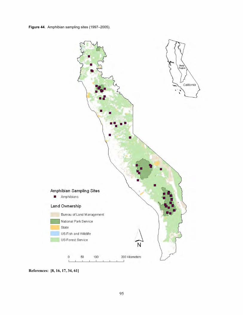
95

Figure 44. Amphibian sampling sites (1997–2005).

References: [8, 16, 17, 34, 61]

96

5. Potential Ecosystem Impacts in the SNSC Region Table 7 lists SNSC ecosystem indicators, potential ecosystem impacts, and the air toxics that have been linked to ecosystem impacts. The potential impacts of air toxics on organisms have been more commonly documented in laboratory studies. However, in some cases, these impacts have also been documented in the field. We highlight below three types of ecosystem impacts.

5.1. Bioaccumulation The bioaccumulation of air toxics has been documented in both aquatic and terrestrial ecosystems in the SNSC region (Table 7). The effects of bioaccumulation of air toxics in ecosystems include: fish concentrations that exceed human and piscivorous wildlife consumption thresholds (including piscivorous fish), biomagnification in piscivorous and insectivorous bird species, and ecosystem level impacts (including changes in the aquatic and terrestrial ecosystem structure). Ultimately, the result of bioaccumulation of organic air toxics and methylmercury in individual organisms can lead to reproductive disruption and immune suppression. In addition, WACAP documented that the bioaccumulation of methylmercury in fish was linked to the presence of macrophage aggregates in fish kidney and spleen, including in brook trout collected from SEKI [1, 4].

Less is known about the potential impacts of bioaccumulation in SNSC terrestrial ecosystems. Although air toxics are generally less bioavailable in terrestrial ecosystems than in aquatic ecosystems, the concentrations of air toxics in litter-fall and soils can be quite high and pesticide concentrations can approach concentrations that are applied to crops [1]. Potentially, these high concentrations could impact the microbial community structure of SNSC soils and other terrestrial organisms, such as songbirds.

5.2. Reproductive Disruption Several air toxics, including DDTs, chlordanes, endosulfans, and PCBs, have been shown to act as endocrine disruptors in laboratory studies. Endocrine disruption may result in intersex fish (fish with the presence of both male and female reproductive structures in the same animal) and/or elevated concentrations of the estrogen-responsive protein vitellogenin [1, 76]. WACAP identified intersex male cutthroat trout and brook trout with elevated vitellogenin concentrations with frequencies of 9–33% in Rocky Mountain and Glacier national parks [1, 76]. However, SEKI fish did not show evidence of intersex or elevated vitellogenin concentrations [1, 76].

Fish collected from YOSE (4 females, 5 males, and 1 intersex male from Mildred Lake) and LAVO (4 females, 4 males, and 0 intersex male from Summit Lake) were analyzed for the same list of organic air toxics as WACAP and the presence or absence of intersex was determined in each of the fish (Figure 5) [35]. Out of a total of 53 fish collected from five different U.S. national parks (Great Sand Dunes, GRSA; Lassen Volcanic, LAVO; Rocky Mountain, ROMO; Wrangell-St. Elias, WRST; and Yosemite, YOSE) and analyzed for the organic air toxics, 8 fish were intersex males. Seven intersex males were collected from ROMO and one intersex male was collected from YOSE [35].

These studies suggest that the Rocky Mountain region has a higher incidence of intersex males than the SNSC region. The reason for this is unknown and cannot be simply linked to the concentration of endocrine disrupting air toxics in the fish because male fish collected from the SNSC region had similar concentrations to intersex male fish collected from the Rocky Mountain region (Figure 5). In addition,

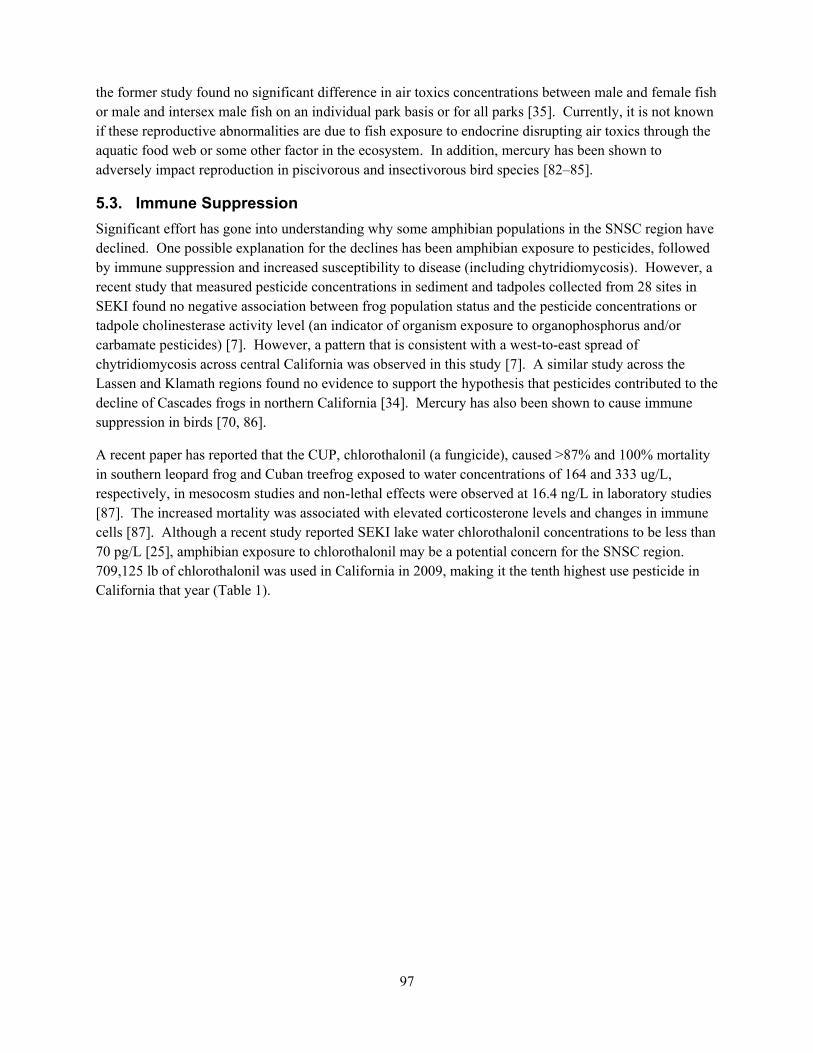
97

the former study found no significant difference in air toxics concentrations between male and female fish or male and intersex male fish on an individual park basis or for all parks [35]. Currently, it is not known if these reproductive abnormalities are due to fish exposure to endocrine disrupting air toxics through the aquatic food web or some other factor in the ecosystem. In addition, mercury has been shown to adversely impact reproduction in piscivorous and insectivorous bird species [82–85].

5.3. Immune Suppression Significant effort has gone into understanding why some amphibian populations in the SNSC region have declined. One possible explanation for the declines has been amphibian exposure to pesticides, followed by immune suppression and increased susceptibility to disease (including chytridiomycosis). However, a recent study that measured pesticide concentrations in sediment and tadpoles collected from 28 sites in SEKI found no negative association between frog population status and the pesticide concentrations or tadpole cholinesterase activity level (an indicator of organism exposure to organophosphorus and/or carbamate pesticides) [7]. However, a pattern that is consistent with a west-to-east spread of chytridiomycosis across central California was observed in this study [7]. A similar study across the Lassen and Klamath regions found no evidence to support the hypothesis that pesticides contributed to the decline of Cascades frogs in northern California [34]. Mercury has also been shown to cause immune suppression in birds [70, 86].

A recent paper has reported that the CUP, chlorothalonil (a fungicide), caused >87% and 100% mortality in southern leopard frog and Cuban treefrog exposed to water concentrations of 164 and 333 ug/L, respectively, in mesocosm studies and non-lethal effects were observed at 16.4 ng/L in laboratory studies [87]. The increased mortality was associated with elevated corticosterone levels and changes in immune cells [87]. Although a recent study reported SEKI lake water chlorothalonil concentrations to be less than 70 pg/L [25], amphibian exposure to chlorothalonil may be a potential concern for the SNSC region. 709,125 lb of chlorothalonil was used in California in 2009, making it the tenth highest use pesticide in California that year (Table 1).

98

Table 7. Potential ecosystem impacts from air toxics in SNSC.

Ecosystem Indicators Potential Ecosystem Impact Which Air Toxics?

Vegetation

Bioaccumulation[1, 69] Deposition to terrestrial ecosystem

through litter-fall[1] Potential effects on soil microbe

population[1] Re-release from forest fires[32]

Pesticides[1, 69] PCBs[1] Mercury [1]

Fish

Bioaccumulation[1, 4, 13–15, 33, 35, 45, 76, 77, 88]

Possible exceedances of human health and wildlife health consumption guidelines[1, 13–15, 35]

Enhanced vitellogenin and intersex in male fish[1, 35, 76]

Reduced reproduction[1, 88] Macrophage aggregates in kidney and

spleen of fish[1, 4] Changes in behavior and development

[88]

Pesticides[1, 13–15, 33, 35, 45, 76]

PBDE flame retardants [1, 13] PCBs [1, 14, 15, 33, 35, 50] Mercury[1, 4, 14, 15, 77, 88] Endocrine disrupting

compounds[1, 13, 76]

Amphibians

Bioaccumulation[7, 8, 16, 17, 33] Decreased growth and development[78] External abnormalities Impaired reproduction Immune suppression Depressed cholinesterase activity[7, 11,

78] Death[78, 87]

Pesticides[7–10, 16, 17, 33, 34, 78, 87]

PCBs [8, 16, 33, 34] Mercury [61, 89]

Birds

Bioaccumulation [79, 82–85, 90–92] Impaired reproduction [82–85, 93] Motor skill impairment [82] Changes in neurochemical receptors

and enzymes [94] Immune Suppression [70, 86]

Mercury [70, 79, 82–86, 90–92, 94]

Pesticides [93]

Ecosystem Dynamics Bioaccumulation[1] Reduced Reproduction[1] Disruption of food web[1] Change in ecosystem structure[1]

Pesticides[1] Mercury

Reference numbers for the relevant literature are given in brackets above.

99

6. Recommendations 1. Expand future analyte lists to include more CUPs, especially those that have been measured in

other remote ecosystems and are used in California. These CUPs include: pendimethalin, metolachlor, dimethoate, carbaryl, myclobutanil, propiconazole, linuron, methyl parathion, metribuzin, atrazine, phorate, disulfoton, dimethenamid, alachlor, ethion, terbufos, imidan, and cyanazine (Table 1).

2. Continue to measure HUPs, PCBs, and mercury in fish collected from the SNSC region in future studies and use this information to inform the public of any potential risks associated with consumption of fish from this region.

3. Compare and analyze the differences between the OEHHA and EPA fish consumption thresholds for the protection of human health. The SNSC Steering Committee can then recommend thresholds for use within the SNSC region and lands.

4. Develop fish consumption thresholds for the protection of piscivorous wildlife health in the SNSC region using available data on health effects and the piscivorous wildlife species present in the SNSC region. Wildlife toxicology experts can aid in examining existing concentrations of contaminants in SNSC fish, and other biota, in comparison to relevant impact thresholds.

5. Include PAHs in the analyte suite of SOCs in fish only when potential new PAH point sources are identified or the contribution of urban areas to pollutants in the SNSC region is the focus of the research. PAH concentrations in SNSC fish do not currently exceed consumption guidelines.

6. Stay informed of the literature on the deposition of emerging pollutants to remote ecosystems (including the Arctic) instead of making additional measurements of PBDEs (and PFCs) to SNSC ecosystems, unless consumption guidelines for PBDEs change.

7. Use annual snowpack to estimate the annual input of air toxics to the SNSC ecosystems because it is an important route of atmospheric deposition to SNSC cold, high elevation ecosystems and scavenges a wide array of air toxics from the atmosphere (both gas-phase and particle-phase pollutants and mercury as well as organic air toxics). However, keep in mind that the selection of the proper passive air sampling media (snow, rain, vegetation, and/or man-made passive air sampler) is study dependent.

8. Support additional research, including atmospheric modeling on air toxic source locations within California, in order to improve predictions of spatial variation in air toxics deposition in the SNSC region. Passive air samplers are being developed for mercury and may be of use in the SNSC region for the validation of mercury deposition models.

9. Use fish as an indicator for measuring air toxics in aquatic ecosystems given relevance for human and piscivorous wildlife health. Piscivorous bird species may also be used as an indicator for mercury in aquatic ecosystems.

10. Support additional research to improve the ability to predict spatial variation in air toxics bioaccumulation in aquatic ecosystems within the SNSC region. Examples of this type of research are the mercury ecosystem models being developed for (and beyond) the SNSC region by the USGS and NPS.

11. Support additional research to improve the ability to predict spatial variation in air toxics bioaccumulation in terrestrial ecosystems within the SNSC region. Consider soils as an indicator for measuring CUPs, HUPs, and PCBs in terrestrial ecosystems. Insectivorous bird species may be used as an indicator for mercury in terrestrial ecosystems.

12. Include more sampling sites to model toxic air contaminant deposition for the SNSC region using chemical concentrations in snow. Improve spatial distribution of sites across the SNSC region, particularly for areas beyond YOSE and SEKI boundaries.

100

7. Outreach and Education Communicating the facts of contaminant presence, threats, and effects in the Sierra Nevada–Southern Cascades (SNSC) region is essential to fostering awareness about the issues. Developing and distributing a common interagency message through communication products creates a foundation for an environmentally-informed culture, including decision-makers. Social and environmental responsibilities are powerful components in ecological stewardship and are essential to reducing contaminant concerns (and other environmental threats) in the region and beyond.

There are numerous outreach avenues and products to consider, many of which are contingent on what audience the product intends to serve. The SNSC Contaminant Workshop held in 2009 and its subsequent meeting report (http://www.nature.nps.gov/air/Studies/air_toxics/wacap/snWorkshop/docs/SNSCC_Meeting_Report_8-31-09.pdf) described possible options. The SNSC Toxics Group, the interagency contaminants group that grew out of the workshop and continued coordinating related contaminant efforts (including the development of this SNSC Research & Monitoring Report), discussed how best to communicate findings from the SNSC Report, and developed the below list of outreach products. Table 8 is a guideline for suggested products (but is not meant to indicate the intended completion of all products).

http://www.nature.nps.gov/air/Studies/air_toxics/wacap/snWorkshop/docs/SNSCC_Meeting_Report_8-31-09.pdf

http://www.nature.nps.gov/air/Studies/air_toxics/wacap/snWorkshop/docs/SNSCC_Meeting_Report_8-31-09.pdf

101

Table 8. Outreach products for communicating threats from contaminants in the SNSC.

Outreach Product Description Audience Projected Date of

Completion Responsible Parties

Fact Sheet for general public

A 1 -page summary describing contaminants, source and transport of contaminants in the region, related threats to human and wildlife health, and what individuals and society in general can do about it.

Visitors to parks, forests, refuges, state lands, etc.; general public

Draft: Sept. 2012 Final: Nov. 2012

FWS (C. Johnson) FS (T. Procter) NPS (C. Flanagan) State (B. Brodberg) + interpretive writer/editors

Fact Sheet for regulators/ policy makers

1–2 page summary of the Report, with more technical description of contaminants, source and transport of contaminants in the region, related threats to human and wildlife health, and how policy/regulation can help to address it.

Agencies, policy-makers; CARB, scientists

Draft: Sept. 2012 Final: Nov. 2012

FWS (C. Johnson) FS (T. Procter) NPS (C. Flanagan) State (B. Brodberg)

Webinar

Interagency, online 1–2 hour meeting where PIs of SNSC Report present integral information regarding report, answering questions regarding how staff should handle the findings

SNSC Committee members and interested agency staff Aug./Sept. 2012

NPS (J. Rocchio/C. Flanagan) PIs (Nanus/Simonich)

Webpages Layered information allowing users to drill down for increasingly complex and area-specific information

Visitors to parks, forests, refuges, state lands, etc. General public including students, teachers; scientists.

2012

NPS FS FWS State (Monitoring Council, and/or SWAMP)

WebMap

An interactive, dynamic map hosted on-line that spatially integrates data regarding SNSC air toxics sample locations compiled as a result of the SNSC Report. Data from Pacific Northwest to be included.

Wide-ranging: agencies; policy-makers; California Air Resources Board (CARB); interested public; scientists

2012 NPS (C. Flanagan) PIs (Nanus/Simonich)

Podcast A 2–3 minute script about air toxics in the region that is storyboarded and available online.

Visitors to parks, forests, refuges, state lands, etc. General public including students, teachers; scientists.

2012 NPS (Elizabeth Munding) Others (?)

102

Outreach Product Description Audience Projected Date of

Completion Responsible Parties

Training materials for agency staff

Fact sheets and webinars; and in addition, to elucidate certain themes, topics, and analogies: images, references, maps, talking points, etc.

Public information officers; outreach and educational-outreach staff; interpretive rangers/naturalists; wilderness rangers

2012–on an as needed basis

NPS FS FWS State (Bob Brodberg)

Educational curriculum

Specific lessons and materials for a series of grades tied directly to the most recent CA State curriculum standards.

Teachers, school districts, students in a range of grades. 2012–2013

NPS FS FWS State

Wayside exhibits Information integrated into thematic, interpretive outdoor panels in locations that are relevant to the topic.

visitors to parks, forests, refuges, state lands, etc. 2013 Park interpreters/designers.

Contract fabricators.

Interactive Module

A computer program that illustrates and conceptualizes contaminant sources in the region, transport, and threats to the ecosystem. Such a program could be linked into current interactive, air quality-related kiosks (e.g. SEKI) or accessed via the internet

Dependent upon venue of deployment: visitors to parks, forests, refuges, state lands, etc.; If via the internet, wide-ranging: policy-makers; general public including scientists, students, teachers; scientists.

2013–?

NPS (J. Winchester, or other agency interpretive specialist) + NPS science communicators, interpretive writers

103

8. Next Steps Summarized below is a list of recommended actions and suggested methods regarding a contaminants research strategy for the SNSC region. Both actions and methods from the report can be considered in future project design phases.

8.1. Recommended Actions Continue to measure HUPs, PCBs, and mercury in fish collected from the SNSC region in future

studies and apply this information in order to inform the public of any potential risks associated with consumption of fish from this region.

Support additional research to improve the ability to predict spatial variation in air toxics bioaccumulation in aquatic ecosystems within the SNSC region. An example of this type of research is the mercury sensitivity model being developed for national parks, including the SNSC region, by the USGS and NPS.

Support additional research to improve the ability to predict spatial variation in air toxics bioaccumulation in terrestrial ecosystems within the SNSC region. Consider soils as an indicator for measuring CUPs, HUPs, and PCBs in terrestrial ecosystems. Insectivorous bird species may be used as an indicator for mercury in terrestrial ecosystems.

Support additional research, including atmospheric modeling on air toxic source locations within California in order to improve predictions of spatial variation in air toxics deposition in the SNSC region. Passive air samplers are being developed for mercury and may be of use in the SNSC region for the validation of mercury deposition models.

Develop fish consumption thresholds for the protection of piscivorous wildlife health in the SNSC region using available data on health effects and the piscivorous wildlife species present in the SNSC region. Wildlife toxicology experts can aid in examining existing concentrations of contaminants in SNSC fish, and other biota, in comparison to relevant impact thresholds.

Compare and analyze the differences between the OEHHA and EPA fish consumption thresholds for the protection of human health. The SNSC Steering Committee can then recommend thresholds for use within the SNSC region and lands.

8.2. Suggested Methods Use annual snowpack to estimate the annual input of air toxics to the SNSC ecosystems. Because

it is an important route of atmospheric deposition to SNSC cold, high elevation ecosystems and scavenges a wide array of air toxics from the atmosphere (both gas-phase and particle-phase pollutants and mercury as well as organic air toxics). However, the selection of the proper passive air sampling media (snow, rain, vegetation, and/or man-made passive air sampler) is study dependent.

Use fish as an indicator for measuring air toxics in aquatic ecosystems given relevance for human and piscivorous wildlife health. In instances where fish collections are too logistically difficult or populations are too sensitive to sample, consider dragonfly larvae as a surrogate for mercury contamination. Piscivorous bird species may also be used as an indicator for mercury in aquatic ecosystems.

Include PAHs in their measurements only when potential new PAH point sources are identified or the contribution of urban areas to pollutants in the SNSC region is the focus of the research, because PAH concentrations in SNSC fish do not currently exceed consumption guidelines.

104

Expand future analyte lists to include more CUPs, especially those that have been measured in other remote ecosystems and are used in California. These CUPs include: pendimethalin, metolachlor, dimethoate, carbaryl, myclobutanil, propiconazole, linuron, methyl parathion, metribuzin, atrazine, phorate, disulfoton, dimethenamid, alachlor, ethion, terbufos, imidan, and cyanazine (Table 1).

Stay informed of the literature on the deposition of emerging pollutants to remote ecosystems (including the Arctic) instead of making additional measurements of PBDEs (and PFCs) to SNSC ecosystems, unless consumption guidelines for PBDEs change.

The issue of where to sample, that includes a rigorous statistical design, should be employed. For example, identifying 50 random sites to sample would permit extrapolation, with known confidence, to the entire study area. One could identify all permanent lakes greater than, for example, 2 ha in area as the population of interest, and then define a random sample from this set. Moreover, one could spread the sampling period over a 3-year period with a small number of sites (e.g., N=5) sampled every year. This would be reasonable and would provide a good example of temporal variation. Tony Olsen (EPA/NHEERL, phone 541-754-4790) has created such designed for a myriad of successful studies–generally at no cost.

From this report, it is expected that interested organizations and researchers will incorporate the research and monitoring recommendations in subsequent studies of air contaminants in the SNSC region. Such entities can work with the SNSC Steering Committee to take advantage of potential funding sources (Appendix A) and implement components of this report. The SNSC Steering Committee can also assist with distribution of anticipated communication and outreach products.

105

9. Conclusion This report thoroughly assesses existing research and monitoring data for toxic airborne contaminants in ecosystems of California’s Sierra Nevada-Southern Cascades region. The recommendations in the report provide resource managers, regulatory agencies, and the public valuable information about conditions and trends, both spatially and temporally, of toxic airborne contaminants and associated risks to sensitive receptors including humans. Results of the project also reveal data gaps with respect to toxic airborne constituents, exposure to sensitive receptors, and extent of the region covered. This assessment provides impetus to initiate additional air contaminants research and monitoring studies in the SNSC region, and it provides a valuable resource to reference when developing a sampling design for such projects.

106

10. Literature References 1. Landers, D. H.; Simonich, S. L.; Jaffe, D.; Geiser, L.; Campbell, D. H.; Schwindt, A.; Schreck, C.; Kent, M.; Hafner, W.; Taylor, H. E.; Hageman, K.; Usenko, S.; Ackerman, L.; Schrlau, J.; Rose, N.; Blett, T.; Erway, M. M., The Fate, Transport, and Ecological Impacts of Airborne Contaminants in Western National Parks (USA). In U.S. Environmental Protection Agency, ORD, NHEERL, Western Ecology Division, Ed. Corvallis, Oregon, 2008.

2. Landers, D. H.; Simonich, S. M.; Jaffe, D.; Geiser, L.; Campbell, D. H.; Schwindt, A.; Schreck, C.; Kent, M.; Hafner, W.; Taylor, H. E.; Hageman, K.; Usenko, S.; Ackerman, L.; Schrlau, J.; Rose, N.; Blett, T.; Erway, M. M., The Western Airborne Contaminant Assessment Project (WACAP): An Interdisciplinary Evaluation of the Impacts of Airborne Contaminants in Western US National Parks. Environmental Science & Technology 2010, 44, (3), 855–859.

3. Flanagan, C., Sierra Nevada-Southern Cascades Contaminants (SNSCC) Workshop Meeting Report-A Strategy for Science and Outreach. In Division, N.-A. R., Ed. National Park Service: 2009.

4. Schwindt, A. R.; Fournie, J. W.; Landers, D. H.; Schreck, C. B.; Kent, M. L., Mercury concentrations in Salmonids from western U.S. national parks and relationships with age and macrophage aggregates (vol 42, pg 1365, 2008). Environmental Science & Technology 2008, 42, (8), 3118–3118.

5. Hageman, K. J.; Simonich, S. L.; Campbell, D. H.; Wilson, G. R.; Landers, D. H., Atmospheric deposition of current-use and historic-use pesticides in snow at national parks in the Western United States. Environmental Science & Technology 2006, 40, (10), 3174–3180.

6. Hageman, K. J.; Hafner, W. D.; Campbell, D. H.; Jaffe, D. A.; Landers, D. H.; Simonich, S. L. M., Variability in Pesticide Deposition and Source Contributions to Snowpack in Western US National Parks. Environmental Science & Technology 2010, 44, (12), 4452–4458.

7. Bradford, D. F.; Knapp, R. A.; Sparling, D. W.; Nash, M. S.; Stanley, K. A.; Tallent-Halsell, N. G.; McConnell, L. L.; Simonich, S. M., Pesticide Distributions and Population Declines of California, USA, Alpine Frogs, Rana Muscosa and Rana Sierrae. Environmental Toxicology and Chemistry 2011, 30, (3), 682–691.

8. Bradford, D. F.; Stanley, K.; McConnell, L. L.; Tallent-Halsell, N. G.; Nash, M. S.; Simonich, S. M., Spatial Patterns of Atmospherically Deposited Organic Contaminants at High Elevation in the Southern Sierra Nevada Mountains, California, USA. Environmental Toxicology and Chemistry 2010, 29, (5), 1056–1066.

9. Davidson, C., Declining downwind: Amphibian population declines in california and historical pesticide use. Ecological Applications 2004, 14, (6), 1892–1902.

10. Davidson, C.; Knapp, R. A., Multiple stressors and amphibian declines: Dual impacts of pesticides and fish on yellow-legged frogs. Ecological Applications 2007, 17, (2), 587–597.

11. Sparling, D. W.; Fellers, G. M.; McConnell, L. L., Pesticides and amphibian population declines in California, USA. Environmental Toxicology and Chemistry 2001, 20, (7), 1591–1595.

12. Wania, F.; Daly, G. L., Organic contaminants in mountains. Environmental Science & Technology

2005, 39, (2), 385–398.

107

13. Ackerman, L. K.; Schwindt, A. R.; Koch, D. C.; Blett, T. F.; Schreck, C. B.; Kent, M. L.; Landers, D. H.; Simonich, S. L. M., Atmospherically deposited PBDEs, pesticides, PCBs, and PAHs in Western US National Park fish: Concentrations and consumption guidelines. Environmental Science &

Technology 2008, 42, (7), 2334–2341.

14. Lim, L.; Brodberg, R.; Gassel, M.; Klasing, S., Health Advisory and Safe Eating Guidelines for Fish from Donner Lake (Nevada County, CA). In Pesticide and Environmental Toxicology Branch, O. o. E. H. H. A., California Environmental Protection Agency, Ed. Sacramento, CA, 2011.

15. Davis, J. A.; Melwani, A. R.; Bezalel, S. N.; Hunt, J. A.; Ichikawa, G.; Bonnema, A.; Heim, W.; Crane, D.; Swenson, S.; Lamerdin, C.; Stephenson, M., Contaminants in Fish from California Lakes and Reservoirs, 2007–2008: Summary Report on a Two-Year Screening Survey. A Report of the Surface Water Ambient Monitoring Program (SWAMP). In Board, C. S. W. R. C., Ed. Sacramento, CA, 2010.

16. Angermann, J. E.; Fellers, G. M.; Matsumura, F., Polychlorinated biphenyls and toxaphene in Pacific tree frog tadpoles (Hyla regilla) from the California Sierra Nevada, USA. Environmental

Toxicology and Chemistry 2002, 21, (10), 2209–2215.

17. Fellers, G. M.; McConnell, L. L.; Pratt, D.; Datta, S., Pesticides in mountain yellow-legged frogs (Rana muscosa) from the Sierra Nevada Mountains of California, USA. Environmental Toxicology and

Chemistry 2004, 23, (9), 2170–2177.

18. Jaffe, D.; Strode, S., Sources, fate and transport of atmospheric mercury from Asia. Environmental

Chemistry 2008, 5, (2), 121–126.

19. Rothenberg, S. E.; Mckee, L.; Gilbreath, A.; Yee, D.; Connor, M.; Fu, X. W., Wet deposition of mercury within the vicinity of a cement plant before and during cement plant maintenance. Atmospheric

Environment 2010, 44, (10), 1255–1262.

20. Finley, B. D.; Swartzendruber, P. C.; Jaffe, D. A., Particulate mercury emissions in regional wildfire plumes observed at the Mount Bachelor Observatory. Atmospheric Environment 2009, 43, (38), 6074–6083.

21. Rothenberg, S. E.; Kirby, M. E.; Bird, B. W.; DeRose, M. B.; Lin, C. C.; Feng, X. B.; Ambrose, R. F.; Jay, J. A., The impact of over 100 years of wildfires on mercury levels and accumulation rates in two lakes in southern California, USA. Environmental Earth Sciences 2010, 60, (5), 993–1005.

22. Gustin, M. S.; Coolbaugh, M. F.; Rytuba, J. J., Annual emissions of mercury to the atmosphere from natural sources in Nevada and California. Environmental Geology 2002, 42, (4), 338–349.

23. Vicars, W. C.; Sickman, J. O., Mineral dust transport to the Sierra Nevada, California: Loading rates and potential source areas. Journal of Geophysical Research-Biogeosciences 2011, 116.

24. Aston, L. S.; Seiber, J. N., Fate of summertime airborne organophosphate pesticide residues in the Sierra Nevada mountains. Journal of Environmental Quality 1997, 26, (6), 1483–1492.

25. Bradford, D. F.; Heithmar, E. M.; Tallent-Halsell, N. G.; Momplaisir, G. M.; Rosal, C. G.; Varner, K. E.; Nash, M. S.; Riddick, L. A., Temporal Patterns and Sources of Atmospherically Deposited Pesticides in Alpine Lakes of the Sierra Nevada, California, USA. Environmental Science & Technology

2010, 44, (12), 4609–4614.

108

26. LeNoir, J. S.; McConnell, L. L.; Fellers, G. M.; Cahill, T. M.; Seiber, J. N., Summertime transport of current-use pesticides from California's Central Valley to the Sierra Nevada Mountain Range, USA. Environmental Toxicology and Chemistry 1999, 18, (12), 2715–2722.

27. Mast, M. A.; Alvarez, D. A.; Zaugg, S., Deposition and Accumulation of Airborne Organic Comtaminants in Yoesmite National Park, California, 2008–09. Environ. Tox. Chem. 2012, 31, (3), 524–533.

28. McConnell, L. L.; LeNoir, J. S.; Datta, S.; Seiber, J. N., Wet deposition of current-use pesticides in the Sierra Nevada mountain range, California, USA. Environmental Toxicology and Chemistry 1998, 17, (10), 1908–1916.

29. Zabik, J. M.; Seiber, J. N., Atmospheric Transport of Organophosphate Pesticides from California Central Valley to the Sierra–Nevada Mountains. Journal of Environmental Quality 1993, 22, (1), 80–90.

30. Summary of Pesticide Use Report Data 2009. In California Environmental Protection Agency, D. o. P. R., Ed. Sacramento, CA, 2010.

31. Primbs, T.; Piekarz, A.; Wilson, G.; Schmedding, D.; Higginbotham, C.; Field, J.; Simonich, S. M., Influence of Asian and Western United States urban areas and fires on the atmospheric transport of polycyclic aromatic hydrocarbons, polychlorinated biphenyls, and fluorotelomer alcohols in the Western United States. Environmental Science & Technology 2008, 42, (17), 6385–6391.

32. Genualdi, S. A.; Killin, R. K.; Woods, J.; Wilson, G.; Schmedding, D.; Simonich, S. L. M., Trans-Pacific and Regional Atmospheric Transport of Polycyclic Aromatic Hydrocarbons and Pesticides in Biomass Burning Emissions to Western North America. Environmental Science & Technology 2009, 43, (4), 1061–1066.

33. Datta, S.; Hansen, L.; McConnell, L.; Baker, J.; LeNoir, J.; Seiber, J. N., Pesticides and PCB contaminants in fish and tadpoles from the Kaweah River basin, California. Bulletin of Environmental

Contamination and Toxicology 1998, 60, (6), 829–836.

34. Davidson, C.; Stanley, K.; Simonich, S. M., Contaminant Residues and Declines of the Cascades Frog (Rana cascadae) in the California Cascades, USA. Environ. Tox. Chem. 2012, in press.

35. Simonich, S. L.; Schrlau, J.; Schreck, C.; Kent, M., Extent of Endocrine Disruption in Fish of the Western and Alaskan National Parks. In University, O. S., Ed. National Park Service: Corvallis, Oregon, 2011.

36. U.S. Environmental Protection Agency, O. o. W., Office of Science and Technology, Guidance for Assessing Chemical Contaminant Data for Use in Fish Advisories. In Washington, D.C., 2000.

37. Neal, R.; Segawa, R.; Wofford, P., Pesticide Air Monitoring Network Monitoring Plan. In Regulation, D. o. P., Ed. California, 2010.

38. Hermanson, M. H.; Isaksson, E. H.; Teixeira, C.; Muir, D. C. G.; Compher, K. M.; Li, Y. F.; Igarashi, I.; Kamiyama, K., Current-use and legacy pesticide history in the Austfonna ice cap, Svalbard, Norway. Environmental Science & Technology 2005, 39, (21), 8163–8169.

39. Raina, R.; Hall, P.; Sun, L. N., Occurrence and Relationship of Organophosphorus Insecticides and Their Degradation Products in the Atmosphere in Western Canada Agricultural Regions. Environmental

Science & Technology 2010, 44, (22), 8541–8546.

109

40. Mast, M. A.; Foreman, W. T.; Skaates, S. V., Current-use pesticides and organochlorine compounds in precipitation and lake sediment from two high-elevation national parks in the Western United States. Archives of Environmental Contamination and Toxicology 2007, 52, (3), 294–305.

41. Hoferkamp, L.; Hermanson, M. H.; Muir, D. C. G., Current use pesticides in Arctic media; 2000–2007. Science of the Total Environment 2010, 408, (15), 2985–2994.

42. Muir, D.; Kurt-Karakus, P. B.; Teixeira, C.; Small, J.; Bidleman, T. F., Current-Use Pesticides in Inland Lake Waters, Precipitation, and Air from Ontario, Canada. Environmental Toxicology and

Chemistry 2011, 30, (7), 1539–1548.

43. Ruggirello, R. M.; Hermanson, M. H.; Isaksson, E.; Teixeira, C.; Forsstrom, S.; Muir, D. C. G.; Pohjola, V.; van de Wal, R.; Meijer, H. A. J., Current use and legacy pesticide deposition to ice caps on Svalbard, Norway. Journal of Geophysical Research-Atmospheres 2010, 115.

44. Thurman, E. M.; Cromwell, A. E., Atmospheric transport, deposition, and fate of triazine herbicides and their metabolites in pristine areas at Isle Royale National Park. Environmental Science & Technology

2000, 34, (15), 3079–3085.

45. Genualdi, S. A.; Hageman, K. J.; Ackerman, L. K.; Usenko, S.; Simonich, S. L. M., Sources and Fate of Chiral Organochlorine Pesticides in Western Us National Park Ecosystems. Environmental

Toxicology and Chemistry 2011, 30, (7), 1533–1538.

46. Cory, L.; Fjeld, P.; Serat, W., Distribution Patterns of Ddt Residues in Sierra-Nevada Mountains. Pesticides Monitoring Journal 1970, 3, (4), 204-&.

47. Klasing, S.; Brodberg, R., Development of Fish Contaminant Goals and Advisory Tissue Levels for Common Contaminants in California Sport Fish: Chlordane, DDTs, Dieldrin, Methylmercury, PCBs, Selenium, and Toxaphene. In Assessment, C. O. o. E. H. H., Ed. Sacramento, CA, 2008.

48. Blocksom, K. A.; Walters, D. M.; Jicha, T. M.; Lazorchak, J. M.; Angradi, T. R.; Bolgrien, D. W., Persistent organic pollutants in fish tissue in the mid-continental great rivers of the United States. Science

of the Total Environment 2010, 408, (5), 1180–1189.

49. Lazorchak, J. M.; McCormick, F. H.; Henry, T. R.; Herlihy, A. T., Contamination of Fish in Streams of the Mid-Atlantic Region: An Approach to Regional Indicator Selection and Wildlife Assessment. Environ. Tox. Chem. 2003, 22, (3), 545–553.

50. Ohyama, K.; Angermann, J.; Dunlap, D. Y.; Matsumura, F., Distribution of polychlorinated biphenyls and chlorinated pesticide residues in trout in the Sierra Nevada. Journal of Environmental

Quality 2004, 33, (5), 1752–1764.

51. Datta, S.; McConnell, L. L.; Baker, J. E.; Lenoir, J.; Seiber, J. N., Evidence for atmospheric transport and deposition of polychlorinated biphenyls to the Lake Tahoe basin, California-Nevada. Environmental Science & Technology 1998, 32, (10), 1378–1385.

52. Primbs, T.; Wilson, G.; Schmedding, D.; Higginbotham, C.; Simonich, S. M., Influence of Asian and Western United States agricultural areas and fires on the atmospheric transport of pesticides in the Western United States. Environmental Science & Technology 2008, 42, (17), 6519–6525.

53. Simonich, S. M.; Primbs, T.; Piekarz, A.; Wilson, G.; Schmedding, D.; Higginbotham, C.; Field, J., Influence of Asian and Western United States urban areas and fires on the atmospheric transport of

110

polycyclic aromatic hydrocarbons, polychlorinated biphenyls, and fluorotelomer alcohols in the Western United States. Environmental Science & Technology 2008, 42, (17), 6385–6391.

54. Council, N. R., Global Sources of Local Pollution: An Assessment of Long-Range Transport of Key Air Pollutants to and from the United States. In The National Academies Press: Washington, D.C., 2010.

55. Usenko, S.; Hageman, K. J.; Schrlau, J. E.; Geiser, L.; Campbell, D. H.; Appleby, P. G.; Landers, D. H.; Simonich, S. L. M., Sources and Deposition of Polycyclic Aromatic Hydrocarbons to Western US National Parks. Environmental Science & Technology 2010, 44, (12), 4512–4518.

56. Sanders, R. D.; Coale, K. H.; Gill, G. A.; Andrews, A. H.; Stephenson, M., Recent increase in atmospheric deposition of mercury to California aquatic systems inferred from a 300-year geochronological assessment of lake sediments. Applied Geochemistry 2008, 23, (3), 399–407.

57. Heyvaert, A. C.; Reuter, J. E.; Slotton, D. G.; Goldman, C. R., Paleolimnological reconstruction of historical atmospheric lead and mercury deposition at Lake Tahoe, California-Nevada. Environmental


58. Drevnick, P. E.; Shinneman, A. L. C.; Lamborg, C. H.; Engstrom, D. R.; Bothner, M. H.; Oris, J. T., Mercury Flux to Sediments of Lake Tahoe, California-Nevada. Water Air and Soil Pollution 2010, 210, (1–4), 399–407.

59. Gay, D. A.; Prestbo, E. M., Wet deposition of mercury in the US and Canada, 1996–2005: Results and analysis of the NADP mercury deposition network (MDN). Atmospheric Environment 2009, 43, (27), 4223–4233.

60. Fain, X.; Obrist, D.; Pierce, A.; Barth, C.; Gustin, M. S.; Boyle, D. P., Whole-watershed mercury balance at Sagehen Creek, Sierra Nevada, CA. Geochimica Et Cosmochimica Acta 2011, 75, (9), 2379–2392.

61. Bradford, D. F.; Kramer, J. L.; Gerstenberger, S. L.; Tallent-Halsell, N. G.; Nash, M. S., Mercury in Tadpoles Collected from Remote Alpine Sites in the Southern Sierra Nevada Mountains, California, USA. Archives of Environmental Contamination and Toxicology 2012, 62, (1), 135–140.

62. Wiener, J. G.; Knights, B. C.; Sandheinrich, M. B.; Jeremiason, J. D.; Brigham, M. E.; Engstrom, D. R.; Woodruff, L. G.; Cannon, W. F.; Balogh, S. J., Mercury in soils, lakes, and fish in Voyageurs National Park (Minnesota): Importance of atmospheric deposition and ecosystem factors. Environmental


63. Strode, S. A.; Jaegle, L.; Jaffe, D. A.; Swartzendruber, P. C.; Selin, N. E.; Holmes, C.; Yantosca, R. M., Trans-Pacific transport of mercury. Journal of Geophysical Research-Atmospheres 2008, 113, (D15).

64. Agency, U. S. E. P., Water Quality Criterion for the Protection of Human Health: Methylmercury. In EPA, Ed. Washington, D.C., 2001.

65. Beckvar, N.; Dillon, T.; Read, L., Approaches for linking whole-body fish tissue residues of mercury or DDT to biological effects thresholds. Environ. Tox. Chem. 2005, 24, 2094–2105.

66. Dillon, T.; Beckvar, S.; Kern, J., Residue-based dose-response in fish: an analysis using lethality-equivalent endpoints. Environ. Tox. Chem. 2010, 29, 2559–2565.

111

67. Sandheinrich, M. B.; Wiener, J. G., Methylmercury in freshwater fish: recent advances in assessing toxicity of environmentally relevant exposures. In Environmental Contamination in Biota: Interpreting

Tissue Concentrations, 2nd edition, Beyer, W. N.; Meador, J. P., Eds. Taylor and Francis Publishers: Boca Raton, Florida, 2011.

68. Walters, D. M.; Blocksom, K. A.; Lazorchak, J. M.; Jicha, T.; Angradi, T. R.; Bolgrien, D. W., Mercury Contamination in Fish in Midcontinent Great Rivers of the United States: Importance of Species Traits and Environmental Factors. Environmental Science & Technology 2010, 44, (8), 2947–2953.

69. Schrlau, J.; Geiser, L.; Hageman, K.; Landers, D. H.; Simonich, S. L., Comparison of Lichen, Conifer Needles, Passive Air Sampling Devices, and Snowpack as Passive Sampling Media to Measure Semi-Volatile Organic Compounds in Remote Atmospheres. Environ. Sci. Technol. 2011, 45, (24), 10354–10361.

70. Elbert, R.; Anderson, D., Mercury Levels, Reproduction, and Hematology in Western Grebes from Three California Lakes, USA. Environ. Tox. Chem. 1998, 17, (2), 210–213.

71. Schauer, J. J.; Hall, B. D.; Olson, M. L.; Rutter, A. P.; Frontiera, R. R.; Krabbenhoft, D. P.; Gross, D. S.; Yuen, M.; Rudolph, T. M., Atmospheric mercury speciation in Yellowstone National Park. Science of the Total Environment 2006, 367, (1), 354–366.

72. Esperanza, A.; van Mantgem, L., Sierra Nevada Network vital signs monitoring plan: Appendix C. Air quality synthesis for Sierra Nevada Network parks. In National Park Service: Fort Collins, CO, 2008.

73. Gustin, M. S.; Lyman, S. N.; Kilner, P.; Prestbo, E., Development of a passive sampler for gaseous mercury. Atmospheric Environment 2011, 45, (32), 5805–5812.

74. Lyman, S. N.; Gustin, M. S.; Prestbo, E. M., A passive sampler for ambient gaseous oxidized mercury concentrations. Atmospheric Environment 2010, 44, (2), 246–252.

75. Hunt, J.; Markiewicz, D.; Pranger, M., Summary of Toxicity in California Waters: 2001–2009. In Program, C. S. W. A. M., Ed. California Water Boards: 2010.

76. Schwindt, A. R.; Kent, M. L.; Ackerman, L. K.; Simonich, S. L. M.; Landers, D. H.; Blett, T.; Schreck, C. B., Reproductive Abnormalities in Trout from Western US National Parks. Transactions of

the American Fisheries Society 2009, 138, (3), 522–531.

77. Saiki, M. K.; Martin, B. A.; May, T. W.; Alpers, C. N., Mercury concentrations in fish from a Sierra Nevada foothill reservoir located downstream from historic gold-mining operations. Environmental Monitoring and Assessment 2010, 163, (1–4), 313–326.

78. Sparling, D. W.; Fellers, G. M., Toxicity of Two Insecticides to California, USA, Anurans and Its Relevance to Declining Amphibian Populations. Environmental Toxicology and Chemistry 2009, 28, (8), 1696–1703.

79. Eagles-Smith, C. A.; Ackerman, J. T.; Adelsbach, T.; Takekawa, J.; Miles, A.; Keister, R., Mercury Correlations Among Six Tissues for Four Waterbird Species Breeding in San Francisco Bay, California, USA. Environ. Tox. Chem. 2008, 27, (10), 2136–2153.

112

80. Bradford, D. F.; Stanley, K.; Tallent-Halsell, N. G.; Sparling, D. W.; Nash, M. S.; Simonich, S. L., Temporal and Spatial Variation of Atmospherically Deposited Organic Contaminants at High Elevation in Yosemite National Park, California, USA. 2012, in preparation.

81. Usenko, S.; Landers, D. H.; Appleby, P. G.; Simonich, S. L., Current and historical deposition of PBDEs, pesticides, PCBs, and PAHs to Rocky Mountain National Park. Environmental Science &

Technology 2007, 41, (21), 7235–7241.

82. Driscoll, C. T.; Han, Y. J.; Chen, C. Y.; Evers, D. C.; Lambert, K. F.; Holsen, T. M.; Kamman, N. C.; Munson, R. K., Mercury contamination in forest and freshwater ecosystems in the Northeastern United States. Bioscience 2007, 57, (1), 17–28.

83. Eagles-Smith, C. A.; Ackerman, J. T., Developing Impairment Thresholds for the Effects of Mercury on Forster's Tern Reproduction in San Francisco Bay. . In Center, W. E. R., Ed. U.S. Geological Survey: Davis, CA, 2010; pp 1–21.

84. Burgess, N. M.; Meyer, M. W., Methylmercury exposure associated with reduced productivity in common loons. Ecotoxicology 2008, 17, (2), 83–91.

85. Brasso, R. L.; Cristol, D. A., Effects of mercury exposure on the reproductive success of tree swallows (Tachycineta bicolor). Ecotoxicology 2008, 17, (2), 133–141.

86. Hawley, D. M.; Hallinger, K. K.; Cristol, D. A., Compromised immune competence in free-living tree swallows exposed to mercury. Ecotoxicology 2009, 18, (5), 499–503.

87. McMahon, T.; Halstead, N.; Johnson, S.; al, e., The Fungicide Chlorothalonil is Nonlinearly Associated with Corticosterone Levels, Immunity, and Mortality in Amphibians. Environmental Health

Perspectives 2011, On-line.

88. Crump, K. L.; Trudeau, V. L., Mercury-Induced Reproductive Impairment in Fish. Environ. Tox.

Chem. 2009, 28, (5), 895–907.

89. Bergeron, C.; Bodinof, C.; Unrine, J.; Hopkins, W., Mercury Accumulation Along a Contamination Gradient and Nondestructive Indices of Bioaccumulation in Amphibians. Environ. Tox. Chem. 2010, 29, (4), 980–988.

90. Jackson, A. K.; Evers, D. C.; Folsom, S. B.; Condon, A. M.; Diener, J.; Goodrick, L. F.; McGann, A. J.; Schmerfeld, J.; Cristol, D. A., Mercury exposure in terrestrial birds far downstream of an historical point source. Environmental Pollution 2011, 159, (12), 3302–3308.

91. Rimmer, C. C.; Miller, E. K.; McFarland, K. P.; Taylor, R. J.; Faccio, S. D., Mercury bioaccumulation and trophic transfer in the terrestrial food web of a montane forest. Ecotoxicology 2010, 19, (4), 697–709.

92. Ackerman, J. T.; Eagles-Smith, C. A.; Takekawa, J.; Bluso, J.; Adelsbach, T., Mercury Concentrations in Blood and Feathers of Prebreeding Forster's Terns in Relation to Space Use of San Francisco Bay, California, USA, Habitats. Environ. Tox. Chem. 2008, 27, (4), 897–908.

93. Gervais, J.; Rosenberg, D.; Fry, M.; Trulio, L.; Stuerm, K., Burrowing Owls and Agricultural Pesticides: Evaluation of Residues and Risks for Three Populations in California, USA. Environ. Tox.

Chem. 2000, 19, (2), 337–343.

113

94. Scheuhammer, A. M.; Basu, N.; Burgess, N. M.; Elliott, J. E.; Campbell, G. D.; Wayland, M.; Champoux, L.; Rodrigue, J., Relationships among mercury, selenium, and neurochemical parameters in common loons (Gavia immer) and bald eagles (Haliaeetus leucocephalus). Ecotoxicology 2008, 17, (2), 93–101.

95. Evers, D. C.; Jackson, A. K.; Tear, T. H.; Osborne, C. E., Hidden Risk: Mercury in Terrestrial Ecosystems of the Northeast. BRI Report 2012-07. In Biodiversity Research Institute. Gorham, Maine, 2012.

114

Appendix A. SNSC Toxics Funding Plan Several agencies represented by the SNSC Steering Committee (SC) have funding calls during the year for proposals that could apply to environmental contaminants research and monitoring projects. SNSC SC agency representatives identified existing sources of funding which are available annually on a competitive basis (see table below). Agency contact names are also provided. Agencies where no current funding sources were identified are listed in the event future funds become available.

The table below is a list of the existing SC agency funding sources which could be targeted for toxics research and monitoring projects identified in this SNSC Toxics Report. The requirements for each funding source are different and are expected to change over time. Researchers interested in pursuing research and monitoring recommendations in this Report are also encouraged to seek funding from additional non-agency sources.

115

SNSC Toxics Steering Committee Agency Potential Funding Sources

Competitive Funding Sources and Agency Contact

Project Type Due Dates Who’s Eligible Project Length Dollar Limit Years

NPS Consolidated Natural Resources Servicewide Comprehensive Call –Judy Rocchio [email protected]

Climate Change Air Quality-Ecological Effects Biological Resource Division Natural Resources Protection Natural Resource Management Regional Program Block Servicewide and Support Threatened & Endangered Species Ocean Resource Stewardship USGS WQ Funding

2011 October through January

National Park Units & Research Partners

3 years $50–500K FY 2013–2016

NPS Air Resources Division End of Year Funds –Tamara Blett [email protected]

Must relate to “effects” of air pollution (O3, S, N, toxics, Mercury) in ecosystems. Emphasize survey, sampling, or other process to answer the early-stage question “is air pollution causing a problem to park resources” OR for synthesizing and communicating air pollution effects information for the public.

2012 March through June


1 year or less $10–$40K 2012

NPS Inventory and Monitoring (I&M) Program –Penny Latham [email protected]

Resource must be listed as a park “vital sign”. I&M Network level (multi-park) projects will be given highest priority.

2012


Varies Varies 2014

FS–Trent Procter [email protected]

USGS–Mike Majewksi [email protected]

Included in the NPS Servicewide Comprehensive call above

FWS Environmental Contaminants On and Off Refuge Investigations –Cathy Johnson [email protected]

Analytical measurements of environmental contaminants on and off FWS refuges. 2012

Agencies and Universities

Multi-year $100K to $450K 2012

mailto:[email protected]






116

Competitive Funding Sources and Agency Contact

Project Type Due Dates Who’s Eligible Project Length Dollar Limit Years

FWS Landscape Conservation Cooperative (LCC) –Cathy Johnson [email protected]

Toxics research opportunities may exist in the future through this multi-agency coordination effort.

Throughout year

Specific to Individual LCCs

annual Small 2012

EPA–Patti Tenbrook [email protected]

NRCS–Ted Strauss [email protected]

San Joaquin Valley APCD –David Nunes [email protected]

San Francisco Water Power and Sewer, San Francisco Public Utilities Commission. –Bob Brodberg [email protected]

City of San Francisco is collecting fish as part of a larger effort To study water, sediments, and plankton in the Tuolumne River watershed. The ideal study would be to add enough $$ one time to analyze chemicals other than mercury in the fish collected by the Park Service in Yosemite.

2011 Yosemite NP and Partners

1 or 2 years varies 2012

Surface Water Ambient Monitoring Program (SWAMP) Bioaccumulation Oversite Group (BOG) –Bob Brodberg [email protected]

As part of a statewide evaluation of inland waters. SWAMP is interested in monitoring high elevation lakes to determine whether they meet water quality objectives. Studies must fit within their monitoring goals. They have not established goals for 2012.

2011

Agencies, Universities and Research Partners

Multi-year varies 2012







117

Appendix B. SNSC Steering Committee Tamara Blett, Ecologist, Air Resources Division (ARD), National Park Service (NPS)

Colleen Flanagan, Ecologist, ARD, NPS

Judy Rocchio, Regional Air Quality Coordinator, Pacific West Region, NPS

Annie Esperanza, Air Quality Specialist, Sequoia and Kings Canyon National Parks

Leland Tarnay, Air Resource Specialist, Yosemite National Park

Janet Cole, Vegetation Ecologist, Lassen Volcanic National Park

Trent Procter, Regional Air quality Program Manager, Region 5, US Forest Service

Ted Strauss, Director of Air Quality, Climate Change, and Energy Conservation, USDA-Natural Resources Conservation Service

Cathy Johnson, Contaminants Specialist, US Fish and Wildlife Service, Region 8

Michael Majewski, Research Chemist, US Geological Survey, Western Region

Patti TenBrook, Life Scientist, US Environmental Protection Agency, Region 9

Robert Brodberg, Chief, Fish and Water Quality Evaluation Section, Office of Environmental Health Hazard Assessment, California Environmental Protection Agency (Cal/EPA)

Lynn Baker, Air Pollution Specialist, California Air Resources Board

David Nunes, Senior Air Quality Specialist, San Joaquin Valley Unified Air Pollution Control District.

118

Appendix C. Laboratories used in previous studies Laboratories used to measure air toxics in environmental media. This list is not exhaustive. Oregon State University Corvallis, Oregon USA Staci L. Simonich, Ph.D., [email protected]; (541)737-9194 Measurement of organic air toxics in various media (snow, vegetation, sediment, fish, amphibians, lake water, etc), made WACAP measurements, as well as other measurements in NPS fish and amphibians. USGS-NRP Trace Element Environmental Analytical Chemistry Project Boulder, CO Howard Taylor, [email protected], (303)541-3007 Measurement of metals in various media for WACAP. EPA, Willamette Research Station Analytical Laboratory Corvallis, OR Dixon Landers, [email protected], (541)754-4427 Measurement of mercury in various media for WACAP. U.S. Geological Survey National Water Quality Laboratory Lakewood, Colorado Measurement of CUPs, HUPS, PCBs and PBDEs in snow, rain, lichen, sediment and zooplankton California Department of Fish and Game Water Pollution Control Laboratory Rancho Cordova, CA Trace organics in fish muscle tissue analysis for SWAMP project. Moss Landing Marine Laboratory Moss Landing, CA Total mercury and selenium in fish muscle tissue for SWAMP project. U.S. Geological Survey Forest and Rangeland Ecosystem Science Center 3200 SW Jefferson Way Corvallis OR, 97331 Measurement of mercury in environmental media. U.S. Geological Survey Wisconsin Water Science Center Middleton, WI Measurement of mercury in various media for USGS.




119

Appendix D. Annotated Bibliography The Spatial Extent of Air Toxics Data in the SNSC Region

An annotated bibliography has been developed to include select scientific reports, journal articles, and online databases with available air toxics data for the SNSC region. The available data described here were used to create associated GIS layers for evaluating the spatial and temporal extent of existing data on surface water, sediment, snow, fish, vegetation, and amphibian declines that may be linked to exposure of air toxic contaminants. This section summarizes the extent of existing air toxics data from multiple sources within public lands of the SNSC region with a focus on Wilderness Areas, and includes sources of data on historic and current use pesticides, mercury, PCB’s, and contaminants. This annotated bibliography only includes publications with available data and accurate sample location information that were used to create the maps included in this report. Numbers correspond to Figures 9B and 9C in the report.

Reports and Journal Articles. Multiple scientific reports and journal articles discuss air toxics in the study area and provide supplementary tables that include location information.

1) Ackerman, L.K.; Schwindt, A.R.; Koch, D.C.; Blett, T.F.; Schreck, C.B.; Kent, M.L.; Landers, D.H.; Simonich, S.L.M., Atmospherically deposited PBDEs, pesticides, PCBs, and PAHs in Western US National Park fish: Concentrations and consumption guidelines. Environmental Science &

Technology 2008, 42, (7), 2334–2341. Emerald and Pear Lakes in SEKI were sampled to evaluate PBDEs, pesticides, PCBs, and PAHs in fish. This data is included in the WACAP database.

2) Angermann J.E., Fellers, G.M., Matsumura, F., Polychlorinated biphenyls and toxaphene in Pacific

tree frog tadpoles (Hyla regilla) from the California Sierra Nevada, USA. Environmental Toxicology

and Chemistry 2002, 21, (10), 2209–2215. Data from 21 sites throughout Sierra Nevada on PCBs and toxaphene in tadpoles. Decreases in concentrations of PCBs and toxaphene with elevation are shown.

3) Aston, L.S., Seiber, J.N., 1997. Fate of Summertime Airborne Organophosphate Pesticide Residues in the Sierra Nevada Mountains. Journal of Environmental Quality 1997, 26, (6), 1483–1492.

Organophosphate pesticide residues were evaluated in air and pine needles at three sites along an elevational transect in the southern Sierra Mountains. The three sites sampled in 1994 include Lindcove, Ash Mountain, and Lower Kaweah.

4) Bradford, D.F.; Heithmar, E.M.; Tallent-Halsell, N.G.; Momplaisir, G.M.; Rosal, C.G.; Varner, K.E.;

Nash, M.S.; Riddick, L.A., Temporal Patterns and Sources of Atmospherically Deposited Pesticides in Alpine Lakes of the Sierra Nevada, California, USA. Environmental Science & Technology 2010, 44, (12), 4609–4614.

Temporal data were collected from mid-June to mid-October 2003 at four SEKI lakes to evaluate the magnitude and temporal variation of atmospherically deposited pesticides in lake water at two sites located near the San Joaquin valley and two sites located further away. Of a total of 41

120

pesticide compounds analyzed, seven were detected, and four were evaluated for temporal variation.

5) Bradford, D. F.; Stanley, K.; McConnell, L. L.; Tallent-Halsell, N. G.; Nash, M. S.; Simonich, S. M., Spatial Patterns of Atmospherically Deposited Organic Contaminants at High Elevation in the Southern Sierra Nevada Mountains, California, USA. Environmental Toxicology and Chemistry

2010, 29, (5), 1056–1066.

Twenty-eight water bodies were sampled twice for air, sediment, and tadpoles in 2005 to evaluate the spatial distribution of organic contaminants at high elevations in SEKI.

6) Cory, L., Fjeld, P., Serat, W., Distribution patterns of DDT residues in the Sierra Nevada mountains. Pesticides Monitoring Journal 1970, 3:204–211.

A generally north to south increase in pesticide concentrations in the Sierra Nevada mountains is observed, along with lower concentrations on the east slope in comparison to the west slope. The paper reports elevated DDE concentrations in areas associated with DDT spraying to control forest pests within the Sierra Nevada.

7) Fellers, G. M.; McConnell, L. L.; Pratt, D.; Datta, S., Pesticides in mountain yellow-legged frogs (Rana muscosa) from the Sierra Nevada Mountains of California, USA. Environmental Toxicology

and Chemistry 2004, 23, (9), 2170–2177.

Samples were collected from 2 basins in SEKI (Sixty Lakes Basin and Tablelands) in 1997 to evaluate pesticides in mountain yellow-legged frogs (Rana muscosa).

8) Hageman, K.J.; Hafner, W.D.; Campbell, D.H.; Jaffe., D.A., Landers, D.H., Simonich, S., Variability in Pesticide Deposition and Source Contributions to Snowpack in Western U.S. National Parks. Environmental Science & Technology 2010, 44, 4452–4458.

Snow samples were collected at two sites in SEKI, Emerald and Pear Lake, from 2003–2005. Samples were analyzed for current-use and historic-use pesticides to evaluate variability in pesticide deposition.

9) Hunt, J.; Markiewicz, D.; Pranger, M., Summary of Toxicity in California Waters: 2001–2009. In

SWAMP, Ed. California Water Boards: 2010. California toxics data and toxicity report and available fish tissue data collected from 2001 to 2009 by the Surface Water Ambient Monitoring Program (SWAMP) in the SNSC region.

10) Krabbenhoft, D.P., Olsen, M.L., Dewild, J.F., Clow, D.W., Striegl, R.G., Dornblaser, M.M.,

Vanmetre, P., Mercury Loading and Methylmercury Production and Cycling in High-Altitude Lakes from the Western United States, Water, Air, Soil Pollution: Focus 2, 2002, 233–249.

Surface water samples were collected during the summer of 1999 from YOSE, SEKI, and LAVO to evaluate mercury loading in high-elevation lakes of the western US. Data are available online at http://co.water.usgs.gov/projects/CO335/CO335.html.

11) Landers, D.H.; Simonich, S.L.; Jaffe, D.; Geiser, L.; Campbell, D.H.; Schwindt, A.; Schreck, C.;

Kent, M.; Hafner, W.; Taylor, H.E.; Hageman, K.; Usenko, S.; Ackerman, L.; Schrlau, J.; Rose, N.;

http://co.water.usgs.gov/projects/CO335/CO335.html

121

Blett, T.; Erway, M.M., The Fate, Transport, and Ecological Impacts of Airborne Contaminants in Western National Parks (USA). In U.S. Environmental Protection Agency, ORD, NHEERL, Western Ecology Division, Ed. Corvallis, Oregon, 2008.

Published data collected from 2002 through 2007 includes air, surface water, sediment, snow, fish, lichen, and conifer needles. WACAP methods have been well developed. Primary sites include two lakes (Emerald and Pear) located 1 km apart in SEKI. Secondary sites include 1 air site and 5 vegetation sites in Yosemite and Lassen National Parks. Six contaminants that were included in the WACAP study were mercury, dieldrin (insecticide), DDT (insecticide), PCBs, chlordane (insecticide), PAHs. The report and associated MS Access database are available on-line at http://nrdata.nps.gov/programs/ard/WACAP Database.zip.

12) LeNoir, J.S., McConnell, L.L., Fellers, G.M., Cahill, T.M., and Seiber, J.N., 1999. Summertime transport of current-use pesticides from California’s central valley to the Sierra Nevada Mountain Range, USA. Environmental Toxicology and Chemistry 1999, 18, (12), 2715–2722.

Air, dry deposition, and surface water samples were collected at different elevations in SEKI in 1996 and 1997 to determine the extent of summertime atmospheric transport of pesticides. Dry deposition or air samples were collected at Lake Kaweah, Ash Mountain, and Lower Kaweah. Surface water samples were collected along an elevation transect at Visalia, Lake Kaweah, Sycamore Creek, Kaweah River, Moro Creek, Crescent Meadow, Tablelands, and Sixty Lakes basin.

13) Lim, L.; Brodberg, R.; Gassel, M.; Klasing, S., Health Advisory and Safe Eating Guidelines for Fish from Donner Lake (Nevada County, CA). In Pesticide and Environmental Toxicology Branch, OEHHA, California Environmental Protection Agency, Ed. Sacramento, CA, 2011.

The report for Donner Lake and associated data on mercury in fish and PCBs is available online: http://www.oehha.ca.gov/fish/so_cal/donner.html. Additional information on the air monitoring network, and list of pesticides being monitored can be accessed at: http://www.cdpr.ca.gov/docs/emon/airinit/air_network.htm. Extensive fish tissue database for Donner Lake.

14) Mast, M. A.; Alvarez, D.A.; Zaugg, S., Deposition and Accumulation of Airborne Organic Comtaminants in Yosemite National Park, California, 2008–09. Environmental Toxicology and

Chemistry 2012, 31, (3), 524–533.

Samples were collected in Yosemite National Park in 2008 and 2009. Wet deposition (12 snow and 1 bulk deposition), 23 lichen samples, 19 lakes (lake surface sediments and lake water) were sampled at different elevations in YOSE and were analyzed for organic contaminants. A sediment core was collected at Tenaya lake.

15) McConnell, L.L.; LeNoir, J. S.; Datta, S.; Seiber, J. N., Wet deposition of current-use pesticides in the Sierra Nevada mountain range, California, USA. Environmental Toxicology and Chemistry 1998, 17, (10), 1908–1916.

Snow samples were collected at Ward Creek (elevation 2,200 m), approximately 2 km east of Ward Peak, west of Lake Tahoe and at Lower Kaweah (elevation 2,000 m) in the Sequoia National Forest to evaluate deposition of current-use pesticides.

http://nrdata.nps.gov/programs/ard/WACAP%20Database.zip

http://www.oehha.ca.gov/fish/so_cal/donner.html

https://email.sfsu.edu/owa/redir.aspx?C=ebbc48db899942e4b3d7db80178c01e1&URL=http%3a%2f%2fwww.cdpr.ca.gov%2fdocs%2femon%2fairinit%2fair_network.htm

122

16) Ohyama, K., Angermann. J.E., Dunlap D.Y., Matsumura, F., Distribution of polychlorinated biphenyls and chlorinated pesticide residues in trout in the Sierra Nevada. Journal of Environmental

Quality 2004, 33, 5, 1752–1764. Data for DDTs, chlordane, toxaphene, and PCBs reported at 10 sites in the northern and central Sierra. PCB concentrations decreased with elevation.

17) Schwindt, A. R.; Fournie, J. W.; Landers, D. H.; Schreck, C. B.; Kent, M., Mercury concentrations

in Salmonids from western U.S. national parks and relationships with age and macrophage aggregates. Environmental Science & Technology 2008, 42, (8), 3118–3118.

18) Simonich, S.L.; Schrlau, J.; Schreck, C.; Kent, M., Extent of Endocrine Disruption in Fish of the

Western and Alaskan National Parks. In University, O. S., Ed. National Park Service: Corvallis, Oregon, 2011.

Measurements of SOCs in 53 fish collected from 5 National Parks including YOSE and LAVO.

19) Zabik, J.M.; Seiber, J.N., Atmospheric Transport of Organophosphate Pesticides from California Central Valley to the Sierra-Nevada Mountains. Journal of Environmental Quality 1993, 22, (1), 80–90.

Winter air and wet-deposition samples were collected along an elevational transect at Lindcove, Three Rivers, Ash Mountain, and Lower Kaweah in 1990 and 1991 to evaluate atmospheric transport of organophosphate pesticides from the Central Valley to the Sierra Nevada.

20) Mast, M.A., 2011. US Geological Survey Unpublished Mercury data, written communication. Lichen samples were collected and analyzed for total mercury at 12 sites in Yosemite National Park. These sites are also included in (12). Mercury concentrations collected and analyzed in snow and surface water for Yosemite National Park.

21) San Francisco Public Utilities Commission (SFPUC), Hetch Hetchy Fish Bioaccumulation Study

Data Summary, Natural Resources and Lands Management Division, Fisheries and Wildlife Section 2011.

SFPUC collected 42 fish samples from Hetch Hetchy reservoir in YOSE in 2009 and analyzed them for mercury contamination to validate the results of SWAMP. Sediment and water samples were also collected and analyzed for mercury.

123

Appendix E. Abbreviations APCD Air Pollution Control District ARB Air Resources Board ARD Air Resources Division (NPS) ATL Advisory Tissue Level (OEHHA) α-HCH alpha-hexachlorocyclohexane BOG Bioaccumulation Oversite Group Cal/EPA California Environmental Protection Agency CUP current use pesticide DDE dichlorodiphenyldichloroethylene (DDT by-product) DDT dichlorodiphenyltrichloroethane EPA US Environmental Protection Agency FCG Fish Contaminant Goals (OEHHA) FF factor-corrected flux FS US Forest Service FWS US Fish & Wildlife Service GC/MS gas chromatographic mass spectrometry GLAC Glacier National Park GRSA Great Sand Dunes National Park & Preserve HCB hexachlorobenzene HUP historic use pesticide HYSPLIT Hybrid Single Particle Lagrangian Integrated Trajectory Model γ-HCH gamma- hexachlorocyclohexane; i.e., lindane IMPROVE Interagency Monitoring of Protected Visual Environments I&M Inventory & Monitoring (NPS) LAVO Lassen Volcanic National Park LCC Landscape Conservation Cooperative MDN Mercury Deposition Network N no data NADP National Atmospheric Deposition Program nd not detected NHEERL National Health and Environmental Effects Research Laboratory (EPA) NI no information nm not measured NOAA National Oceanic and Atmospheric Administration NRCS Natural Resources Conservation Service NPS National Park Service OEHHA Office of Environmental Health Hazard Assessment (Cal/EPA) ORD Office of Research & Development (EPA) PAH polycyclic aromatic hydrocarbon PASD passive air sampling device PBDE polybrominated diphenyl ether PCB polychlorinated biphenyl

124

PFC perfluorinated compound PI principal investigator PPCP pharmaceuticals and personal care products ROMO Rocky Mountain National Park SC Steering Committee SEKI Sequoia & Kings Canyon National Parks SFPUC San Francisco Public Utilities Commission SNSC Sierra Nevada – Southern Cascades SPMD semi-permeable membrane device SWAMP Surface Water Ambient Monitoring Program USDA US Department of Agriculture USGS US Geological Survey WACAP Western Airborne Contaminants Assessment Project WRST Wrangell-St. Elias National Park & Preserve ww wet weight XAD resin (Amberlite XAD) for passive air sampling devices YOSE Yosemite National Park

Sierra Nevada-Southern Cascades (SNSC) Region Air ... · PDF fileSierra Nevada-Southern...

Documents

Transcript of Sierra Nevada-Southern Cascades (SNSC) Region Air ... · PDF fileSierra Nevada-Southern...