Sibling correlations in terms of education, profession and ...

Sibling correlations in terms of education, profession

and earnings, in France

Celine Lecavelier des Etangs-Levallois, Arnaud Lefranc

THEMA - Universite de Cergy-Pontoise

September 16, 2015

Abstract

This paper analyses intergenerational transmission of inequalities in France, estimating sibling

correlations in terms of education, profession and earnings. Data from the French Education-

Training-Employment (FQP) survey are used to investigate similarities between siblings.

Sibling correlations around 0.3 and 0.5 are respectively found for education years and prestige

scores. In terms of annual earnings, estimations lie in between, around 0.4. Evolution in time

and effect of particular familial characteristics are also further investigated.

1 Introduction

The extent of intergenerational transmission of socioeconomic status has interested economists

for decades, as it reflects the level of equality of opportunities inside a society. The degree to

which socioeconomic status is transmitted from one generation to the next indeed captures

the impact family background can have on children’s success in later life: the effect of fac-

tors independent from children’s choices, talents and efforts on their future success. In other

words, it represents to what extent childhood circumstances are reflected in adult life.

As a measure of the degree of intergenerational mobility, empirical studies have often

analyzed the intergenerational elasticity, the regression coefficient relating child’s outcome

to parental one. However the impact of the familial environment can not be restricted to

a single parental characteristic. Sibling correlations thus provide a summary measure of all

effects attributed to factors shared by siblings. It captures the overall impact of growing up

in the same family, including for instance sharing a common neighborhood.

Sibling correlations for various socioeconomic outcomes have been estimated in different

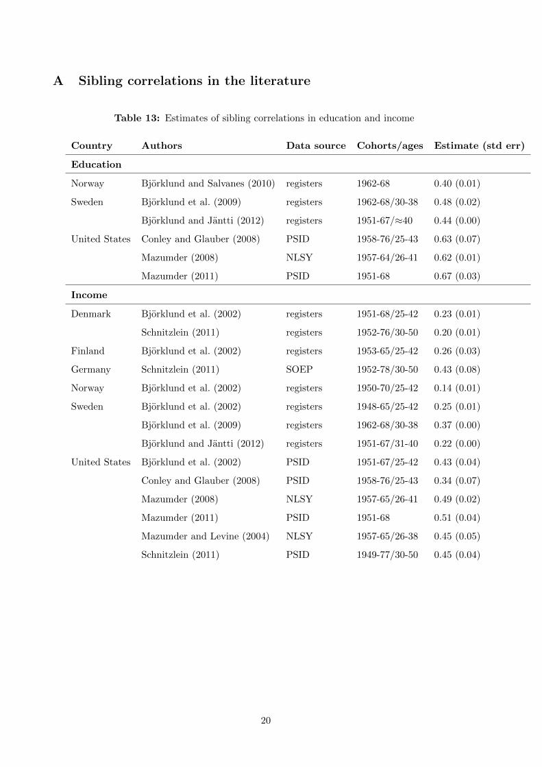
countries. A summary of some recent studies’ results is reported in Table 13, in appendix,

and comparable litterature reviews can be found in Bjorklund and Jantti (2009), Bjorklund

and Salvanes (2010) and Bjorklund and Jantti (2012). In terms of education, sibling corre-

lations from 0.4 for Nordic countries and 0.6 for the United States are found. They amount

around 0.2 for Nordic countries and 0.4 for Germany and the United States, in terms of

income. Nevertheless, if several authors have investigated the cases of these countries, there

is currently no work studying intergenerational transmission of socioeconomic status using

sibling correlations, in France. And this is the gap in the litterature we want to fill with this

paper.

We use data from the French Education-Training-Employment (FQP) survey to estimate

sibling similarities in different socioeconomic outcomes: profession, education and earnings.

And we find sibling correlations around 0.3, 0.4 and 0.5 for education years, annual earnings

and prestige scores respectively. When conducting a study by gender, it appears that same-sex

siblings have more in common than in mixed pairs, for each outcome. Additional parameters

are then investigated, not leading to any clear conclusion toward the evolution in time of

sibling correlations. However concerning the impact of familial composition, closely spaced

siblings are more alike and family size seems to have a positive effect on sibling correlations.

Finally we investigate the effect of parental education and profession but observe no clear

pattern, except for the decrease of sibling correlations in earnings with educational levels of

both parents.

The paper proceeds as follows. Section 2 presents the FQP data. Section 3 describes the

prediction of the three outcomes we further investigate. Section 4 presents the estimation

method of sibling correlations. Section 5 reports the results and Section 6 concludes.

2 Data

The data used in this paper come from the French Education-Training-Employment (FQP)

survey. The targeted individuals are 18 to 65 year old people living in France, yielding a

sample of around 40000 individuals. We use the wave of 2003, in which information on a

randomly selected sibling is available. The wave of 1993 is also used in order to help predicting

years of education and prestige scores for both siblings. Additionally waves of 1970, 1977

and 1985 are used to predict earnings.

For our analysis we select individuals born between 1943 and 1973, which means 30 to 60

years old in 2003. We only keep individuals paired to a sibling. We allow up to 10 years of

age difference between the individual (referred to as ”ego”) and his/her sibling (referred to

2

as ”alter”). Therefore, siblings can be born between 1933 and 1983 and are 20 to 70 years

old in 2003. This choice is made to avoid sampling young people with only older siblings,

and old people with only younger siblings.

Available information concerning gender, birth cohort, education and socio-professional

category for both siblings allows us to investigate sibling correlations in different socio-

economic outcomes. Additional information on the composition of the family - as number

and birth order of brothers/sisters, age difference between ego and alter - and birth cohort,

education, profession of the parents, enable taking various characteristics of the family into

account to investigate their impact on sibling correlations.

Descriptive statistics

First, gender repartition and ages among siblings are reported in Tables 1 and 2 respectively.

The sample counts 21885 pairs of siblings, 5240 of which being pairs of brothers and 5507

pairs of sisters. The remaining 11138 are mixed pairs. Siblings are aged 44 on average, with

an average age difference of 4 years.

Table 1: Descriptive statistics - gender

sex alter

sex ego 0 1 Total

0 5240 5054 10294

1 6084 5507 11591

Total 11324 10561 21885

Table 2: Descriptive statistics - age

Variable Mean Std. Dev. Min Max

age ego 44.265 8.677 30 60

age alter 44.227 9.804 20 70

age diff. 4.276 2.581 0 10

Note: 21885 observations

In Table 3 is reported the repartition of certificates and degrees obtained respectively by

ego and alter. From the bottom to the top, the first category contains people without any

certificate. Then CEP corresponds to a former school leaving certificate, taken at the end

3

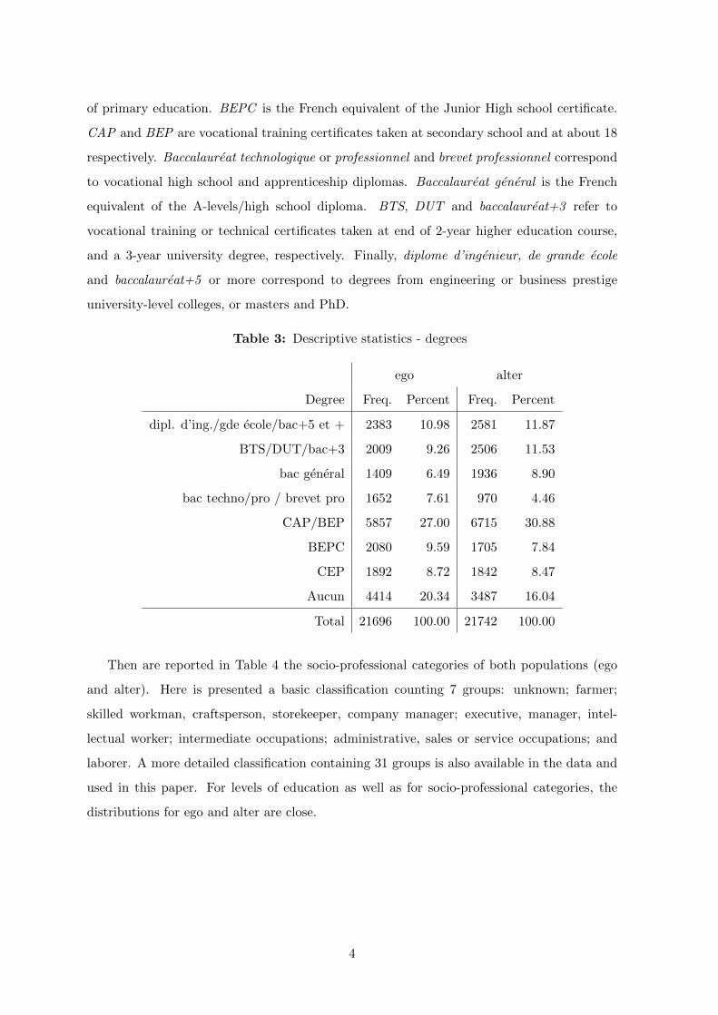
of primary education. BEPC is the French equivalent of the Junior High school certificate.

CAP and BEP are vocational training certificates taken at secondary school and at about 18

respectively. Baccalaureat technologique or professionnel and brevet professionnel correspond

to vocational high school and apprenticeship diplomas. Baccalaureat general is the French

equivalent of the A-levels/high school diploma. BTS, DUT and baccalaureat+3 refer to

vocational training or technical certificates taken at end of 2-year higher education course,

and a 3-year university degree, respectively. Finally, diplome d’ingenieur, de grande ecole

and baccalaureat+5 or more correspond to degrees from engineering or business prestige

university-level colleges, or masters and PhD.

Table 3: Descriptive statistics - degrees

ego alter

Degree Freq. Percent Freq. Percent

dipl. d’ing./gde ecole/bac+5 et + 2383 10.98 2581 11.87

BTS/DUT/bac+3 2009 9.26 2506 11.53

bac general 1409 6.49 1936 8.90

bac techno/pro / brevet pro 1652 7.61 970 4.46

CAP/BEP 5857 27.00 6715 30.88

BEPC 2080 9.59 1705 7.84

CEP 1892 8.72 1842 8.47

Aucun 4414 20.34 3487 16.04

Total 21696 100.00 21742 100.00

Then are reported in Table 4 the socio-professional categories of both populations (ego

and alter). Here is presented a basic classification counting 7 groups: unknown; farmer;

skilled workman, craftsperson, storekeeper, company manager; executive, manager, intel-

lectual worker; intermediate occupations; administrative, sales or service occupations; and

laborer. A more detailed classification containing 31 groups is also available in the data and

used in this paper. For levels of education as well as for socio-professional categories, the

distributions for ego and alter are close.

4

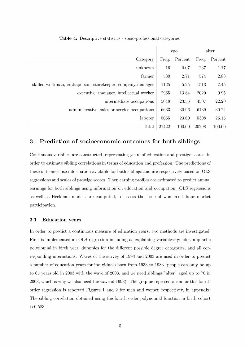
Table 4: Descriptive statistics - socio-professional categories

ego alter

Category Freq. Percent Freq. Percent

unknown 16 0.07 237 1.17

farmer 580 2.71 574 2.83

skilled workman, craftsperson, storekeeper, company manager 1125 5.25 1513 7.45

executive, manager, intellectual worker 2965 13.84 2020 9.95

intermediate occupations 5048 23.56 4507 22.20

administrative, sales or service occupations 6633 30.96 6139 30.24

laborer 5055 23.60 5308 26.15

Total 21422 100.00 20298 100.00

3 Prediction of socioeconomic outcomes for both siblings

Continuous variables are constructed, representing years of education and prestige scores, in

order to estimate sibling correlations in terms of education and profession. The predictions of

these outcomes use information available for both siblings and are respectively based on OLS

regressions and scales of prestige scores. Then earning profiles are estimated to predict annual

earnings for both siblings using information on education and occupation. OLS regressions

as well as Heckman models are computed, to assess the issue of women’s labour market

participation.

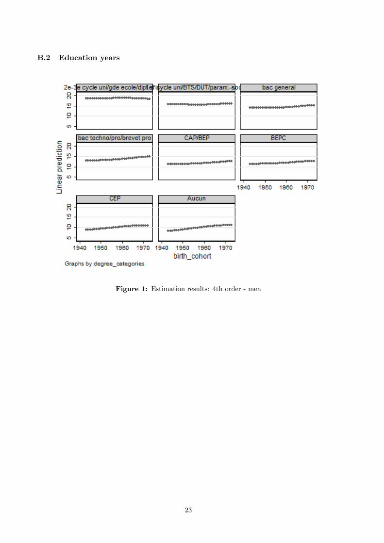
3.1 Education years

In order to predict a continuous measure of education years, two methods are investigated.

First is implemented an OLS regression including as explaining variables: gender, a quartic

polynomial in birth year, dummies for the different possible degree categories, and all cor-

responding interactions. Waves of the survey of 1993 and 2003 are used in order to predict

a number of education years for individuals born from 1933 to 1983 (people can only be up

to 65 years old in 2003 with the wave of 2003, and we need siblings ”alter” aged up to 70 in

2003, which is why we also need the wave of 1993). The graphic representation for this fourth

order regression is reported Figures 1 and 2 for men and women respectivey, in appendix.

The sibling correlation obtained using the fourth order polynomial function in birth cohort

is 0.583.

5

Then a non-parametric specification including dummies for each gender/cohort/degree

category is tested. The sibling correlation resulting from this specification is 0.578 and a

graphic representation is reported in Figures 3 and 4, in appendix. Sibling correlations by

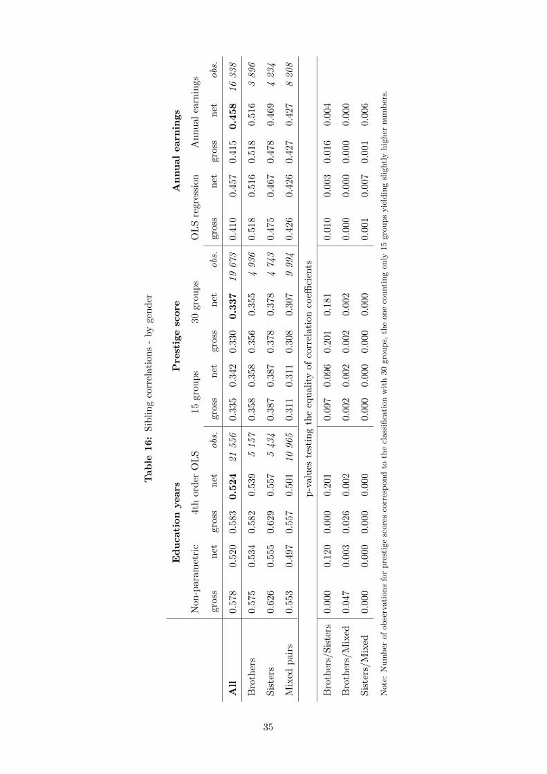
gender for parametric and non-parametric specifications are reported in Table 16 in appendix.

As expected, mixed sibling pairs share less than same-sex siblings, and sisters seem to have

more in common than brothers. Also correlations obtained with the different specifications

are very close.

3.2 Prestige score

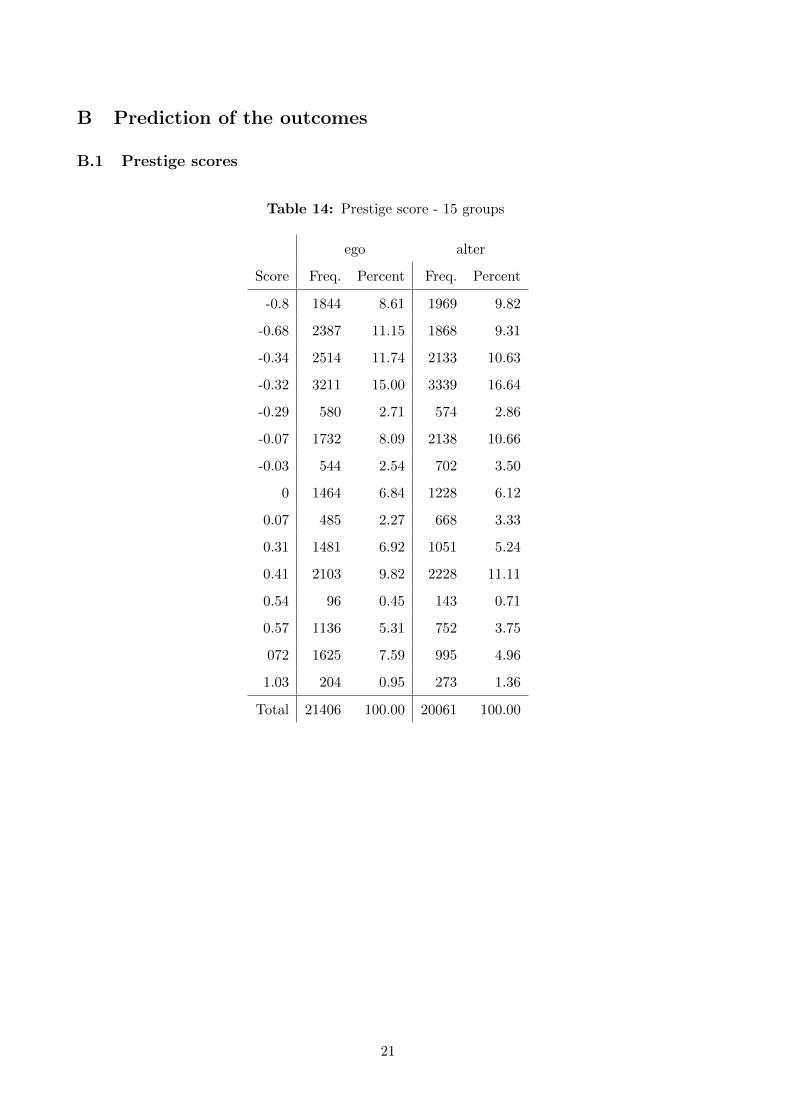
Concerning prestige scores associated with the profession, two different strategies have also

been implemented, based on Chambaz et al. (1998). In their paper, scales of prestige scores

are constructed for different classifications of professions or socio-professional categories. First

we choose to simply aggregate some of the groups from our classification in 30 categories (the

first category being ”unknown” and thus excluded) to fit their classification in 15 categories,

and attribute the corresponding scores to each sibling, the socio-professional category being

available for both. This first classification is presented in Table 14, in appendix.

Then we also want to obtain a more precise scale by attributing a score to each of our

30 groups. Therefore we use the extremely detailed scale of scores attributed to a list of

professions. The profession is however only available for ego in our data, so that we attribute

the weighted mean of the scores (weighted by the frequency of each profession in the groups)

for each of our 30 groups of socio-professional categories, for both siblings. This second

classification is reported in Table 15, in appendix.

The sibling correlations obtained for the classifications with 15 and 30 groups respectively

are 0.335 and 0.330, so these two scales of prestige scores yield again very similar results. More

detailed correlations by gender are presented in Table 16 in appendix. Again the correlations

are higher for same-sex siblings, and also slightly higher for sisters than for brothers.

3.3 Women’s labor force participation

The relatively low participation of women into the labor force can raise an issue. Indeed

prestige scores are attributed according to the last observed socio-economic category. Mostly

for women, this potentially reflects the professional situation in the beginning of a short

career, stopped for instance to raise children. But our interest is in the correlations between

obtainable prestige scores, potentially reached if everybody had always worked.

6

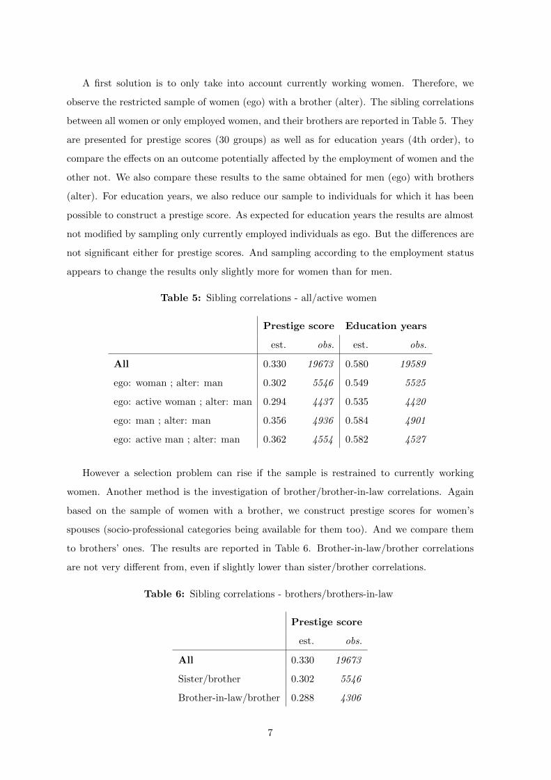
A first solution is to only take into account currently working women. Therefore, we

observe the restricted sample of women (ego) with a brother (alter). The sibling correlations

between all women or only employed women, and their brothers are reported in Table 5. They

are presented for prestige scores (30 groups) as well as for education years (4th order), to

compare the effects on an outcome potentially affected by the employment of women and the

other not. We also compare these results to the same obtained for men (ego) with brothers

(alter). For education years, we also reduce our sample to individuals for which it has been

possible to construct a prestige score. As expected for education years the results are almost

not modified by sampling only currently employed individuals as ego. But the differences are

not significant either for prestige scores. And sampling according to the employment status

appears to change the results only slightly more for women than for men.

Table 5: Sibling correlations - all/active women

Prestige score Education years

est. obs. est. obs.

All 0.330 19673 0.580 19589

ego: woman ; alter: man 0.302 5546 0.549 5525

ego: active woman ; alter: man 0.294 4437 0.535 4420

ego: man ; alter: man 0.356 4936 0.584 4901

ego: active man ; alter: man 0.362 4554 0.582 4527

However a selection problem can rise if the sample is restrained to currently working

women. Another method is the investigation of brother/brother-in-law correlations. Again

based on the sample of women with a brother, we construct prestige scores for women’s

spouses (socio-professional categories being available for them too). And we compare them

to brothers’ ones. The results are reported in Table 6. Brother-in-law/brother correlations

are not very different from, even if slightly lower than sister/brother correlations.

Table 6: Sibling correlations - brothers/brothers-in-law

Prestige score

est. obs.

All 0.330 19673

Sister/brother 0.302 5546

Brother-in-law/brother 0.288 4306

7

3.4 Annual earnings

There is a measure of annual earnings in the wave 2003 of the survey, however only available

for interviewed individuals, not for their siblings. The strategy to obtain earnings for both

siblings is here to estimate earning profiles in a first step with as much information as possible

from all waves from 1970 to 2003 (1970, 1977, 1985, 1993 and 2003). Then in a second step

log of earnings are predicted for both siblings in the database of 2003.

Earning profiles are estimated based on individuals born between years 1933 and 1983

and observed from ages 25 to 55. Age is normalized to zero at age 40, age at which earnings

are predicted, in order to avoid lifecycle bias. Birth cohort is also normalized to zero in

1963 and as explanatory variables for the OLS regression are constructed five groups of birth

cohort covering 10 years each (1933-1942, 1943-1952, 1953-1962, 1963-1972 and 1973-1983).

The two last groups are actually used as only one in the estimation, because the last one

contains individuals born from 1973, too late to predict a satisfactory earning profile, and

stops in fact at year 1978, no individual being younger than 25.

The same dummies corresponding to the different possible degree categories used in the

construction of a continuous measure of education are also here regressors in the prediction

of earnings. For the occupation, the classification in 7 categories is used for interactions with

cohort groups. However categories ”unknown”,”farmer” and ”skilled workman, craftsperson,

storekeeper, company manager” are not kept, because most individuals of the two last ones

are not employed and therefore do not present a satisfactory measure of earnings. A more

detailed classification of socio-professional categories compatible with all waves of the survey

is also used as principal effects. The four remaining categories of the previous classification

contain here 17 categories (only the clerical occupations are additionally excluded).

For men, the regression equation of the log of earnings yi,c,t thus contains different age-

earnings profiles based on education, as well as interactions between cohort groups and both

education and occupation, and can be written:

yi,c,t = αt + φ(Zi,c, c) + ψ(Zi,c, agei,c,t) + ui,c,t,

where i, c, t are indices for individual, birth cohort and date of the survey, Zi,c contains

educational and occupational characteristics, φ captures the effect of these characteristics

depending on the cohort and ψ is a quadratic function of age interacted with education.

Then predicted log of earnings at age 40 in 2003 for both siblings are computed by:

yi,c,t = φ(Zi,c, c).

8

To predict earnings for women, the same OLS regression as well as alternatively the

Heckman model are implemented, in order to handle the issue of their participation into the

labor force. Number of children and spouse’s education level, contained in Wi,c, are then

additionally used to account for the probability of being active, with yi,c,t only observed for

women when the following selection equation is satisfied:

f(Zi,c,Wi,c) + vi,c,t > 0.

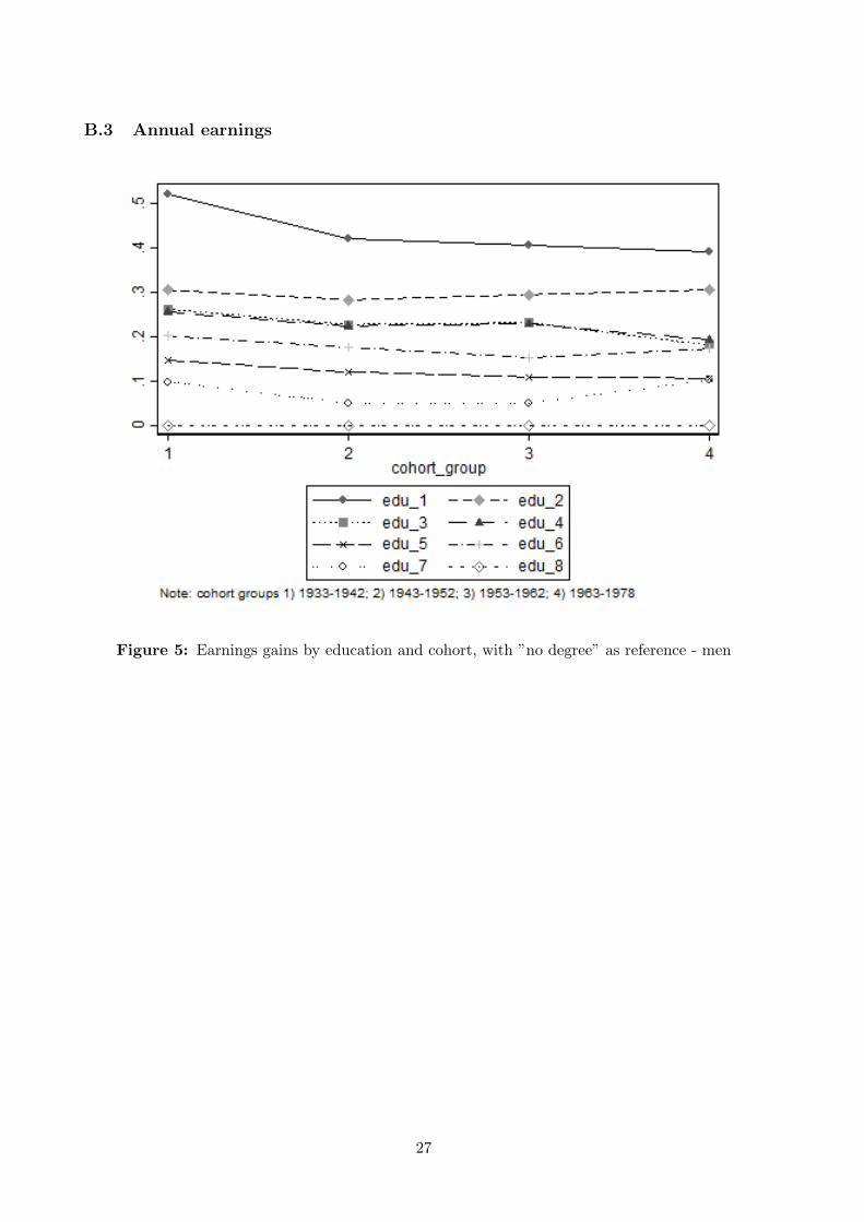
To illustrate these earnings profiles, we represent earnings gains obtained for each level

of education for the different birth cohort groups, as well as the effect of age on earnings also

for each level of education and for the cohort group of reference, individuals born between

1953 and 1962. This is reported respectively in Figures 5 and 6 for men, and for women in

Figures 7 and 8 when earnings are predicted by OLS regression and in Figures 9 and 10 when

Heckman model is used.

The sibling correlations estimated with each model used for the prediction of women’s

earnings are 0.410 and 0.415. Again, there is no big difference between both specifications’

results. More detailed estimates by gender are reported in Table 16 in appendix. Though

correlations are again higher for same-sex pairs than for mixed pairs, here brothers seem to

share a little more than sisters.

4 Estimation of sibling correlations

4.1 Polychoric correlations

First we use the discrete variables of highest completed degree and socioprofessional group

to investigate the association between siblings’ success. Polychoric correlation coefficients

measure the association between two ordinal variables assumed to be determined by a latent

continuous variable following a bivariate normal distribution. We thus use our classification of

degrees in 8 groups (1 to 8 from higher degrees to no degree), and to get an ordinal variable

for occupation, we gather farmers and laborers and obtain the following classification: 1)

executive, manager, intellectual worker; 2) intermediate occupations; 3) skilled workman,

craftsperson, storekeeper, company manager; 4) administrative, sales or service occupations

and 5) farmers and laborers.

9

4.2 Pearson’s correlations

Then in order to estimate sibling linear correlation coefficients, we model an outcome y, here

education years, prestige scores or log of earnings, for individual j in family i:

yi,j = ai + bi,j ,

where ai is a component common to both siblings in family i and bi,j is an individual-

specific component for sibling j in family i. These components are assumed to be independent

of each other, so that the variance of yi,j can be written:

σ2y = σ2

a + σ2b .

In this decomposition, σ2a captures the variance between families, while σ2

b captures the

variance within families. The sibling correlation ρ in which we are interested is the fraction

of the overall variance of the outcome, due to shared background:

ρ = σ2a

σ2a+σ2

b.

A set of complementary controls can be included in the estimation of the model in order

to first purge the outcome of some effects:

yi,j = X ′i,jβ + ai + bi,j = X ′i,jβ + ei,j .

The vector Xi,j here contains a gender dummy, a quartic function of birth cohort, and

all corresponding interactions. And the residuals ei,j from the regression equation, free of

gender and age effects, are then used in order to compute Pearson’s correlations between two

siblings 1 and 2:

ρe1,e2 = cov(e1,e2)σe1σe2

.

Different sibling correlations are computed for same-sex (brother/brother and sister/sister)

and mixed (brother/sister) sibling pairs. We also want to investigate the evolution of the ef-

fect of familial background on siblings’ outcomes over the years. To do so, we split our sample

into three groups, depending on the average parental birth cohort: before 1925, between 1925

and 1935, and after 1935, and estimate different sibling correlations for these different groups.

We also test the same strategy based on average siblings’ birth cohort: before 1954, between

1954 and 1964, and after 1964. Furthermore some familial characteristics are taken into ac-

count, in order to investigate their effect on sibling correlations: age difference between ego

and alter and whether one of them is firstborn, number of siblings, education and profession

of both parents.

10

Correlations on predicted variables

In this paper, we do not estimate correlations on directly observed variables. Instead we first

predict continuous variables to then use them to investigate sibling correlations. And we can

model the latent outcome y as the sum of our predicted variable y and an ε, for each sibling:

yj = yj + εj , with j = e for ego, j = a for alter.

Considering that the distributions are the same for both siblings (that is σye = σya and

σεe = σεa) and that y and ε are independant (so σ2y = σ2

y + σ2ε ), we can find:

ρ(ye, ya) = cov(ye,ya)+cov(εe,εa)σ2y+σ2

ε=

ρ(ye,ya).σ2y+ρ(εe,εa).σ2

ε

σ2y+σ2

ε,

which means:

ρ(ye, ya) = ρ(ye, ya) ⇐⇒ ρ(ye, ya) = ρ(εe, εa).

So if we assume that the sibling association in terms of observable characteristics is the

same as the one concerning non observable characteristics, there is no impact of the use of

predicted variable instead of observed ones, on the estimated sibling correlations.

Inference

Pearson’s correlation coefficient is approximatively normaly distributed for small absolute

values of correlation. However for higher values the distribution is skewed. That is why for

inference issues we use the so-called Fisher’s z transformation to convert Pearson’s ρ to the

normally distributed variable z, with the standard error σz (and number of observations n):

z = 12 ln

1+ρ1−ρ ,

σz = 1√n−3

.

And in order to test whether correlation coefficients from two independant groups 1 and

2 are statistically different:

H0 : ρ1 = ρ2

H1 : ρ1 6= ρ2,

we compute the test statistic U , following the standard normal distribution under the

null hypothesis:

U = z1−z2√1

n1−3+ 1n2−3

.

11

5 Results

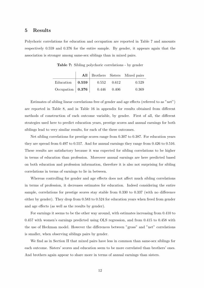
Polychoric correlations for education and occupation are reported in Table 7 and amounts

respectively 0.559 and 0.376 for the entire sample. By gender, it appears again that the

association is stronger among same-sex siblings than in mixed pairs.

Table 7: Sibling polychoric correlations - by gender

All Brothers Sisters Mixed pairs

Education 0.559 0.552 0.612 0.529

Occupation 0.376 0.446 0.406 0.369

Estimates of sibling linear correlations free of gender and age effects (referred to as ”net”)

are reported in Table 8, and in Table 16 in appendix for results obtained from different

methods of construction of each outcome variable, by gender. First of all, the different

strategies used here to predict education years, prestige scores and annual earnings for both

siblings lead to very similar results, for each of the three outcomes.

Net sibling correlations for prestige scores range from 0.307 to 0.387. For education years

they are spread from 0.497 to 0.557. And for annual earnings they range from 0.426 to 0.516.

These results are satisfactory because it was expected for sibling correlations to be higher

in terms of education than profession. Moreover annual earnings are here predicted based

on both education and profession information, therefore it is also not surprising for sibling

correlations in terms of earnings to lie in between.

Whereas controlling for gender and age effects does not affect much sibling correlations

in terms of profession, it decreases estimates for education. Indeed considering the entire

sample, correlations for prestige scores stay stable from 0.330 to 0.337 (with no difference

either by gender). They drop from 0.583 to 0.524 for education years when freed from gender

and age effects (as well as the results by gender).

For earnings it seems to be the other way around, with estimates increasing from 0.410 to

0.457 with women’s earnings predicted using OLS regression, and from 0.415 to 0.458 with

the use of Heckman model. However the differences between ”gross” and ”net” correlations

is smaller, when observing siblings pairs by gender.

We find as in Section II that mixed pairs have less in common than same-sex siblings for

each outcome. Sisters’ scores and education seem to be more correlated than brothers’ ones.

And brothers again appear to share more in terms of annual earnings than sisters.

12

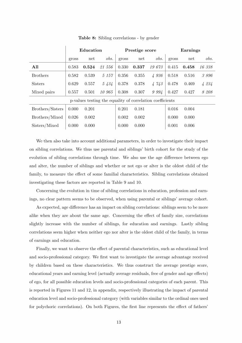
Table 8: Sibling correlations - by gender

Education Prestige score Earnings

gross net obs. gross net obs. gross net obs.

All 0.583 0.524 21 556 0.330 0.337 19 673 0.415 0.458 16 338

Brothers 0.582 0.539 5 157 0.356 0.355 4 936 0.518 0.516 3 896

Sisters 0.629 0.557 5 434 0.378 0.378 4 743 0.478 0.469 4 234

Mixed pairs 0.557 0.501 10 965 0.308 0.307 9 994 0.427 0.427 8 208

p-values testing the equality of correlation coefficients

Brothers/Sisters 0.000 0.201 0.201 0.181 0.016 0.004

Brothers/Mixed 0.026 0.002 0.002 0.002 0.000 0.000

Sisters/Mixed 0.000 0.000 0.000 0.000 0.001 0.006

We then also take into account additional parameters, in order to investigate their impact

on sibling correlations. We thus use parental and siblings’ birth cohort for the study of the

evolution of sibling correlations through time. We also use the age difference between ego

and alter, the number of siblings and whether or not ego or alter is the oldest child of the

family, to measure the effect of some familial characteristics. Sibling correlations obtained

investigating these factors are reported in Table 9 and 10.

Concerning the evolution in time of sibling correlations in education, profession and earn-

ings, no clear pattern seems to be observed, when using parental or siblings’ average cohort.

As expected, age difference has an impact on sibling correlations: siblings seem to be more

alike when they are about the same age. Concerning the effect of family size, correlations

slightly increase with the number of siblings, for education and earnings. Lastly sibling

correlations seem higher when neither ego nor alter is the oldest child of the family, in terms

of earnings and education.

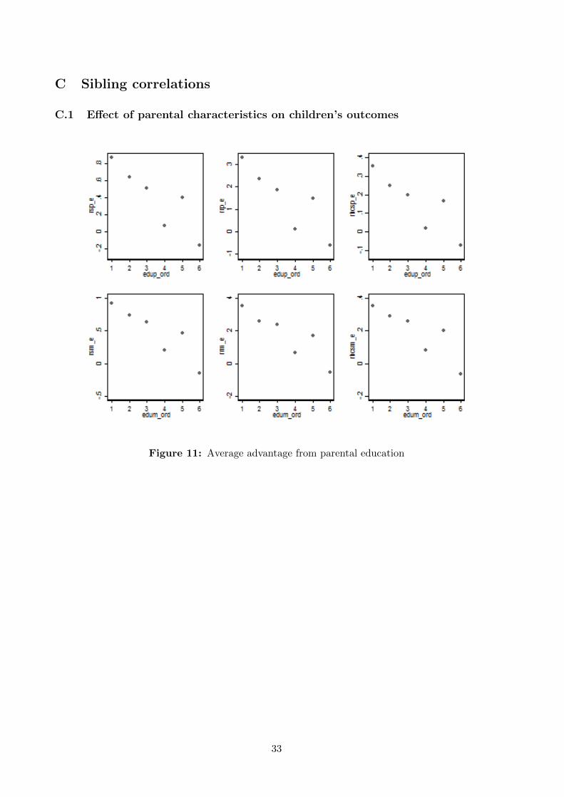
Finally, we want to observe the effect of parental characteristics, such as educational level

and socio-professional category. We first want to investigate the average advantage received

by children based on these characteristics. We thus construct the average prestige score,

educational years and earning level (actually average residuals, free of gender and age effects)

of ego, for all possible education levels and socio-professional categories of each parent. This

is reported in Figures 11 and 12, in appendix, respectively illustrating the impact of parental

education level and socio-professional category (with variables similar to the ordinal ones used

for polychoric correlations). On both Figures, the first line represents the effect of fathers’

13

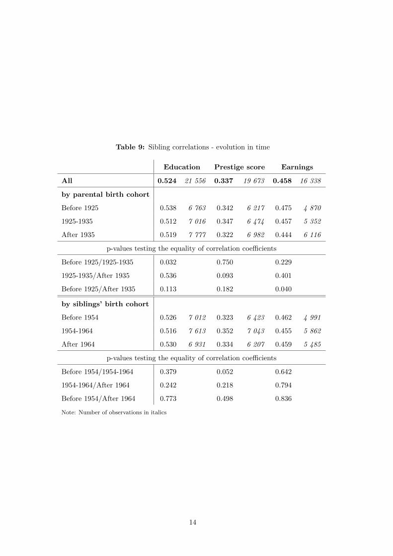
Table 9: Sibling correlations - evolution in time


All 0.524 21 556 0.337 19 673 0.458 16 338

by parental birth cohort

Before 1925 0.538 6 763 0.342 6 217 0.475 4 870

1925-1935 0.512 7 016 0.347 6 474 0.457 5 352

After 1935 0.519 7 777 0.322 6 982 0.444 6 116


Before 1925/1925-1935 0.032 0.750 0.229

1925-1935/After 1935 0.536 0.093 0.401

Before 1925/After 1935 0.113 0.182 0.040

by siblings’ birth cohort

Before 1954 0.526 7 012 0.323 6 423 0.462 4 991

1954-1964 0.516 7 613 0.352 7 043 0.455 5 862

After 1964 0.530 6 931 0.334 6 207 0.459 5 485


Before 1954/1954-1964 0.379 0.052 0.642

1954-1964/After 1964 0.242 0.218 0.794

Before 1954/After 1964 0.773 0.498 0.836

Note: Number of observations in italics

14

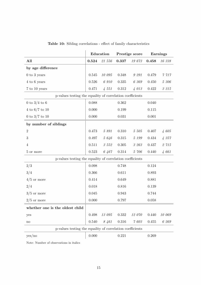
Table 10: Sibling correlations - effect of family characteristics


All 0.524 21 556 0.337 19 673 0.458 16 338

by age difference

0 to 3 years 0.545 10 095 0.348 9 291 0.479 7 717

4 to 6 years 0.526 6 910 0.335 6 369 0.450 5 306

7 to 10 years 0.471 4 551 0.312 4 013 0.422 3 315


0 to 3/4 to 6 0.088 0.362 0.040

4 to 6/7 to 10 0.000 0.199 0.115

0 to 3/7 to 10 0.000 0.031 0.001

by number of siblings

2 0.473 5 891 0.310 5 505 0.407 4 605

3 0.497 5 646 0.315 5 199 0.434 4 357

4 0.511 3 552 0.305 3 263 0.437 2 715

5 or more 0.523 6 467 0.314 5 706 0.440 4 661


2/3 0.098 0.748 0.124

3/4 0.366 0.611 0.893

4/5 or more 0.414 0.649 0.881

2/4 0.018 0.816 0.139

3/5 or more 0.045 0.943 0.744

2/5 or more 0.000 0.797 0.058

whether one is the oldest child

yes 0.498 13 095 0.332 12 070 0.440 10 069

no 0.540 8 461 0.316 7 603 0.455 6 269


yes/no 0.000 0.221 0.269


15

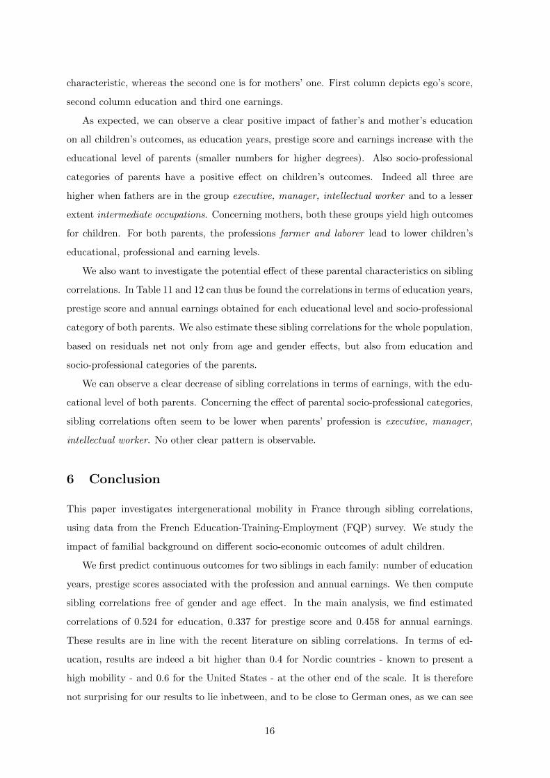
characteristic, whereas the second one is for mothers’ one. First column depicts ego’s score,

second column education and third one earnings.

As expected, we can observe a clear positive impact of father’s and mother’s education

on all children’s outcomes, as education years, prestige score and earnings increase with the

educational level of parents (smaller numbers for higher degrees). Also socio-professional

categories of parents have a positive effect on children’s outcomes. Indeed all three are

higher when fathers are in the group executive, manager, intellectual worker and to a lesser

extent intermediate occupations. Concerning mothers, both these groups yield high outcomes

for children. For both parents, the professions farmer and laborer lead to lower children’s

educational, professional and earning levels.

We also want to investigate the potential effect of these parental characteristics on sibling

correlations. In Table 11 and 12 can thus be found the correlations in terms of education years,

prestige score and annual earnings obtained for each educational level and socio-professional

category of both parents. We also estimate these sibling correlations for the whole population,

based on residuals net not only from age and gender effects, but also from education and

socio-professional categories of the parents.

We can observe a clear decrease of sibling correlations in terms of earnings, with the edu-

cational level of both parents. Concerning the effect of parental socio-professional categories,

sibling correlations often seem to be lower when parents’ profession is executive, manager,

intellectual worker. No other clear pattern is observable.

6 Conclusion

This paper investigates intergenerational mobility in France through sibling correlations,

using data from the French Education-Training-Employment (FQP) survey. We study the

impact of familial background on different socio-economic outcomes of adult children.

We first predict continuous outcomes for two siblings in each family: number of education

years, prestige scores associated with the profession and annual earnings. We then compute

sibling correlations free of gender and age effect. In the main analysis, we find estimated

correlations of 0.524 for education, 0.337 for prestige score and 0.458 for annual earnings.

These results are in line with the recent literature on sibling correlations. In terms of ed-

ucation, results are indeed a bit higher than 0.4 for Nordic countries - known to present a

high mobility - and 0.6 for the United States - at the other end of the scale. It is therefore

not surprising for our results to lie inbetween, and to be close to German ones, as we can see

16

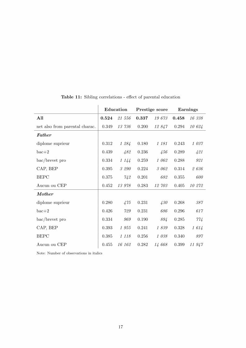
Table 11: Sibling correlations - effect of parental education


All 0.524 21 556 0.337 19 673 0.458 16 338

net also from parental charac. 0.349 13 736 0.200 12 847 0.294 10 624

Father

diplome suprieur 0.312 1 284 0.180 1 181 0.243 1 037

bac+2 0.439 482 0.236 456 0.289 421

bac/brevet pro 0.334 1 144 0.259 1 062 0.288 921

CAP, BEP 0.395 3 290 0.224 3 062 0.314 2 636

BEPC 0.375 742 0.201 682 0.355 600

Aucun ou CEP 0.452 13 978 0.283 12 703 0.405 10 272

Mother

diplome suprieur 0.280 475 0.231 430 0.268 387

bac+2 0.426 729 0.231 686 0.296 617

bac/brevet pro 0.334 969 0.190 894 0.285 774

CAP, BEP 0.393 1 955 0.241 1 839 0.328 1 614

BEPC 0.385 1 118 0.256 1 038 0.340 897

Aucun ou CEP 0.455 16 162 0.282 14 668 0.399 11 947


17

Table 12: Sibling correlations - effect of parental profession


All 0.524 21 556 0.337 19 673 0.458 16 338

net also from parental charac. 0.349 13 736 0.200 12 847 0.294 10 624

Father

farmer 0.435 2 553 0.217 2 368 0.383 1 362

skilled workman, ... 0.455 2 625 0.257 2 381 0.386 1 742

executive, ... 0.370 1 846 0.209 1 686 0.306 1 516

intermediate occupations 0.451 2 829 0.266 2 655 0.335 2 402

administrative, ... 0.444 2 277 0.277 2 089 0.383 1 886

laborer 0.419 8 694 0.256 7 881 0.364 6 905

Mother

farmer 0.411 1 974 0.216 1 876 0.368 1 076

skilled workman, ... 0.420 1 326 0.226 1 220 0.380 887

executive, ... 0.375 292 0.230 260 0.231 231

intermediate occupations 0.446 1 723 0.245 1 606 0.348 1 442

administrative, ... 0.451 5 877 0.286 5 471 0.387 4 897

laborer 0.456 3 038 0.275 2 849 0.387 2 469


18

concerning earnings. For Germany, sibling correlations in terms of income amount around

0.4 as ours, slightly lower than American ones and higher than the results around 0.2 for

Nordic countries.

We also want to measure the effect of some personal and familial characteristics on these

sibling correlations. The mosts significant result is for same-sex sibling pairs to share more

similarities than mixed pairs. We find that family composition as also an impact, sibling cor-

relations for instance increasing with the number of siblings in the family. Finally parental

education and socio-professional levels tend to decrease sibling correlations. Presenting sib-

ling correlations for different socio-economic outcomes, as well as the impact some familial

characteristics can have on them, this paper constitutes a first step to fill the gap in the

literature on sibling correlations in France.

19

A Sibling correlations in the literature

Table 13: Estimates of sibling correlations in education and income

Country Authors Data source Cohorts/ages Estimate (std err)

Education

Norway Bjorklund and Salvanes (2010) registers 1962-68 0.40 (0.01)

Sweden Bjorklund et al. (2009) registers 1962-68/30-38 0.48 (0.02)

Bjorklund and Jantti (2012) registers 1951-67/≈40 0.44 (0.00)

United States Conley and Glauber (2008) PSID 1958-76/25-43 0.63 (0.07)

Mazumder (2008) NLSY 1957-64/26-41 0.62 (0.01)

Mazumder (2011) PSID 1951-68 0.67 (0.03)

Income

Denmark Bjorklund et al. (2002) registers 1951-68/25-42 0.23 (0.01)

Schnitzlein (2011) registers 1952-76/30-50 0.20 (0.01)

Finland Bjorklund et al. (2002) registers 1953-65/25-42 0.26 (0.03)

Germany Schnitzlein (2011) SOEP 1952-78/30-50 0.43 (0.08)

Norway Bjorklund et al. (2002) registers 1950-70/25-42 0.14 (0.01)

Sweden Bjorklund et al. (2002) registers 1948-65/25-42 0.25 (0.01)

Bjorklund et al. (2009) registers 1962-68/30-38 0.37 (0.00)

Bjorklund and Jantti (2012) registers 1951-67/31-40 0.22 (0.00)

United States Bjorklund et al. (2002) PSID 1951-67/25-42 0.43 (0.04)

Conley and Glauber (2008) PSID 1958-76/25-43 0.34 (0.07)

Mazumder (2008) NLSY 1957-65/26-41 0.49 (0.02)

Mazumder (2011) PSID 1951-68 0.51 (0.04)

Mazumder and Levine (2004) NLSY 1957-65/26-38 0.45 (0.05)

Schnitzlein (2011) PSID 1949-77/30-50 0.45 (0.04)

20

B Prediction of the outcomes

B.1 Prestige scores

Table 14: Prestige score - 15 groups

ego alter

Score Freq. Percent Freq. Percent

-0.8 1844 8.61 1969 9.82

-0.68 2387 11.15 1868 9.31

-0.34 2514 11.74 2133 10.63

-0.32 3211 15.00 3339 16.64

-0.29 580 2.71 574 2.86

-0.07 1732 8.09 2138 10.66

-0.03 544 2.54 702 3.50

0 1464 6.84 1228 6.12

0.07 485 2.27 668 3.33

0.31 1481 6.92 1051 5.24

0.41 2103 9.82 2228 11.11

0.54 96 0.45 143 0.71

0.57 1136 5.31 752 3.75

072 1625 7.59 995 4.96

1.03 204 0.95 273 1.36

Total 21406 100.00 20061 100.00

21

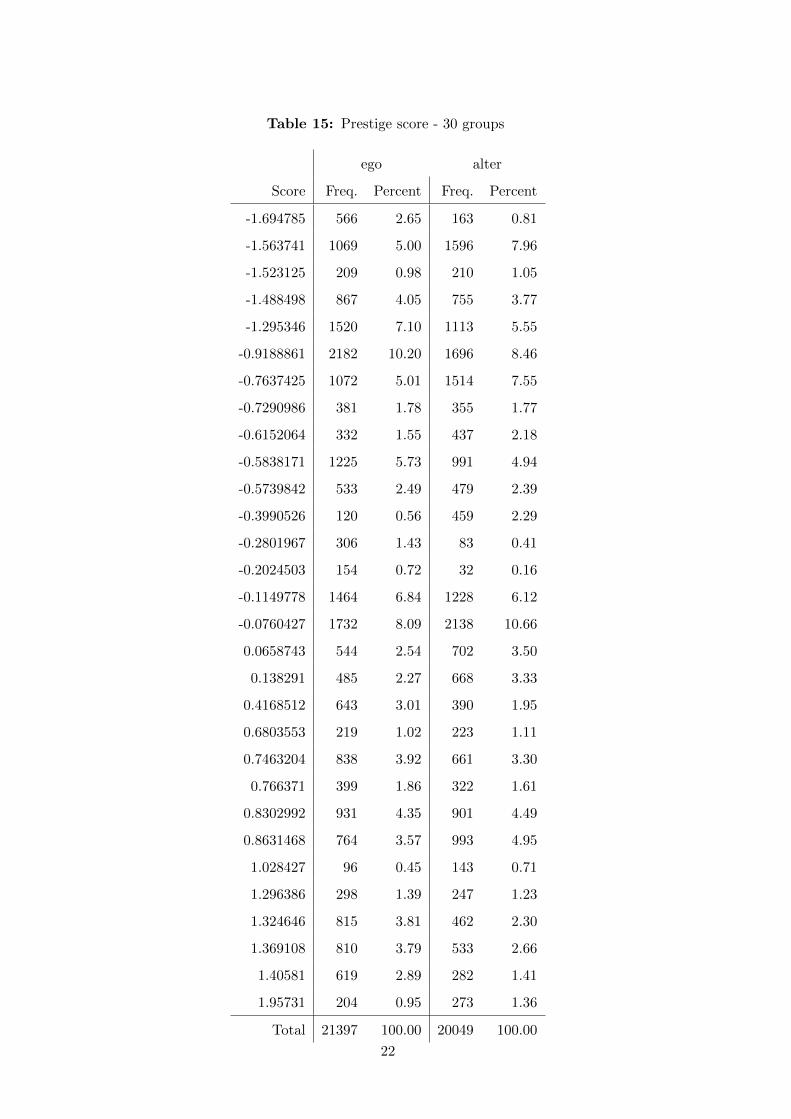
Table 15: Prestige score - 30 groups

ego alter

Score Freq. Percent Freq. Percent

-1.694785 566 2.65 163 0.81

-1.563741 1069 5.00 1596 7.96

-1.523125 209 0.98 210 1.05

-1.488498 867 4.05 755 3.77

-1.295346 1520 7.10 1113 5.55

-0.9188861 2182 10.20 1696 8.46

-0.7637425 1072 5.01 1514 7.55

-0.7290986 381 1.78 355 1.77

-0.6152064 332 1.55 437 2.18

-0.5838171 1225 5.73 991 4.94

-0.5739842 533 2.49 479 2.39

-0.3990526 120 0.56 459 2.29

-0.2801967 306 1.43 83 0.41

-0.2024503 154 0.72 32 0.16

-0.1149778 1464 6.84 1228 6.12

-0.0760427 1732 8.09 2138 10.66

0.0658743 544 2.54 702 3.50

0.138291 485 2.27 668 3.33

0.4168512 643 3.01 390 1.95

0.6803553 219 1.02 223 1.11

0.7463204 838 3.92 661 3.30

0.766371 399 1.86 322 1.61

0.8302992 931 4.35 901 4.49

0.8631468 764 3.57 993 4.95

1.028427 96 0.45 143 0.71

1.296386 298 1.39 247 1.23

1.324646 815 3.81 462 2.30

1.369108 810 3.79 533 2.66

1.40581 619 2.89 282 1.41

1.95731 204 0.95 273 1.36

Total 21397 100.00 20049 100.00

22

B.2 Education years

Figure 1: Estimation results: 4th order - men

23

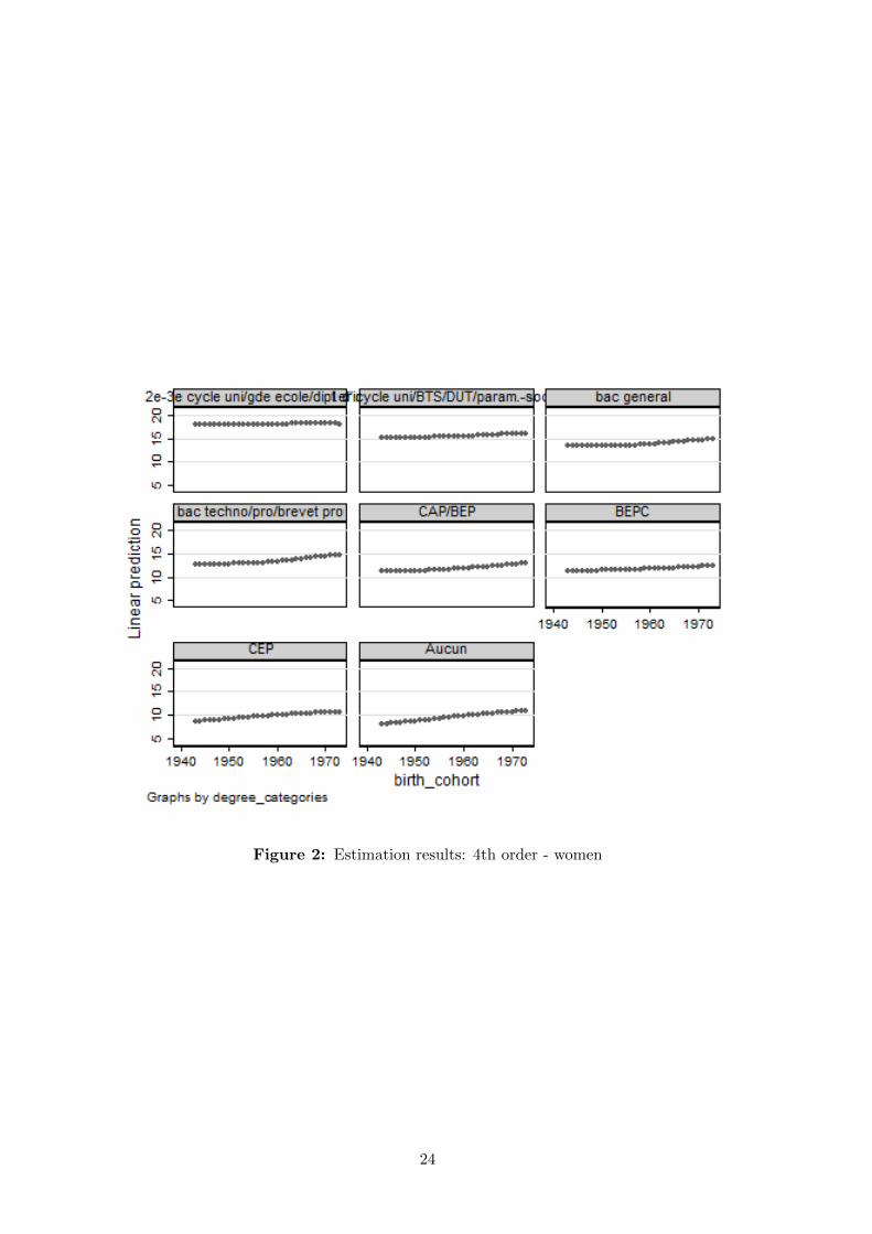
Figure 2: Estimation results: 4th order - women

24

Figure 3: Estimation results: non-parametric specification - men

25

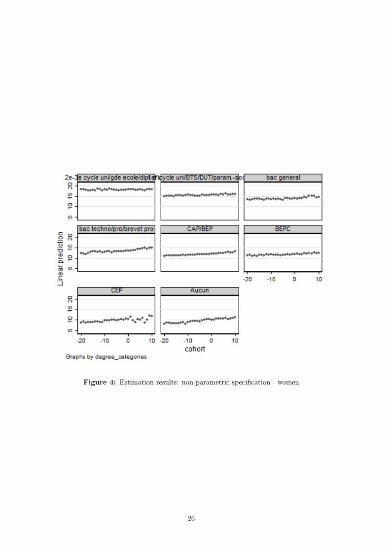
Figure 4: Estimation results: non-parametric specification - women

26

B.3 Annual earnings

Figure 5: Earnings gains by education and cohort, with ”no degree” as reference - men

27

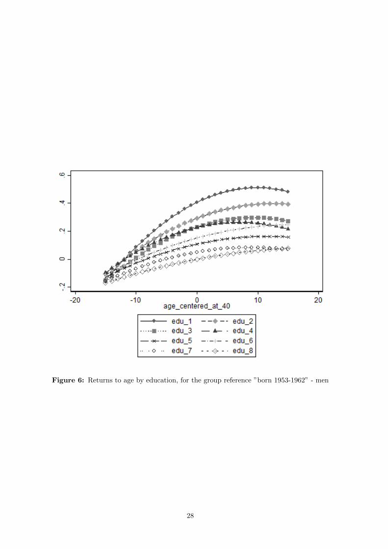
Figure 6: Returns to age by education, for the group reference ”born 1953-1962” - men

28

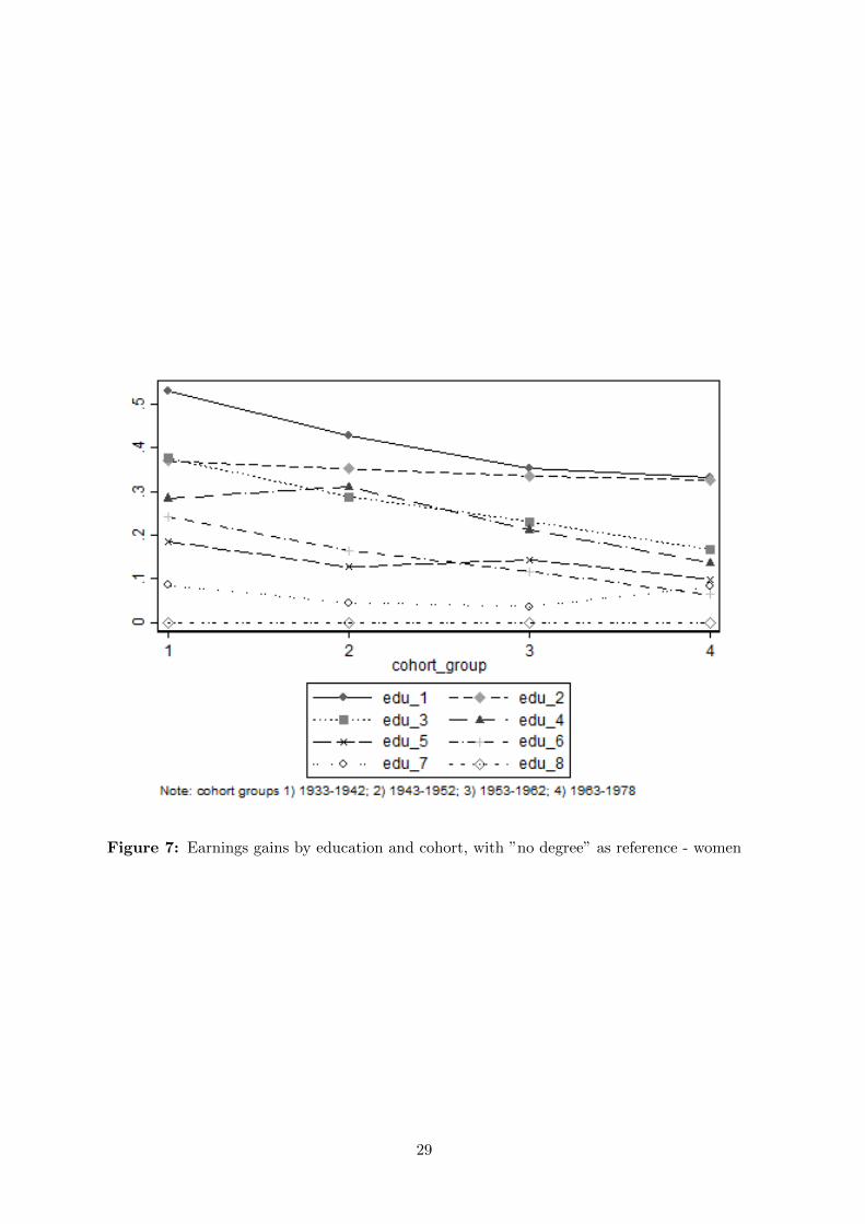
Figure 7: Earnings gains by education and cohort, with ”no degree” as reference - women

29

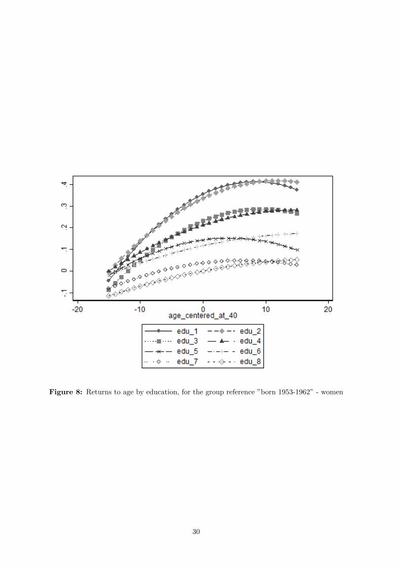
Figure 8: Returns to age by education, for the group reference ”born 1953-1962” - women

30

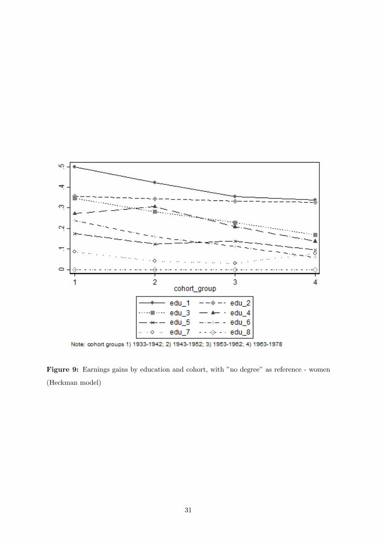
Figure 9: Earnings gains by education and cohort, with ”no degree” as reference - women

(Heckman model)

31

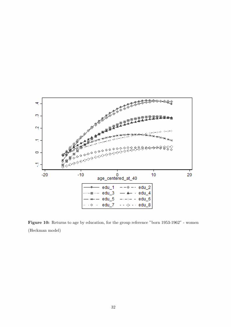
Figure 10: Returns to age by education, for the group reference ”born 1953-1962” - women

(Heckman model)

32

C Sibling correlations

C.1 Effect of parental characteristics on children’s outcomes

Figure 11: Average advantage from parental education

33

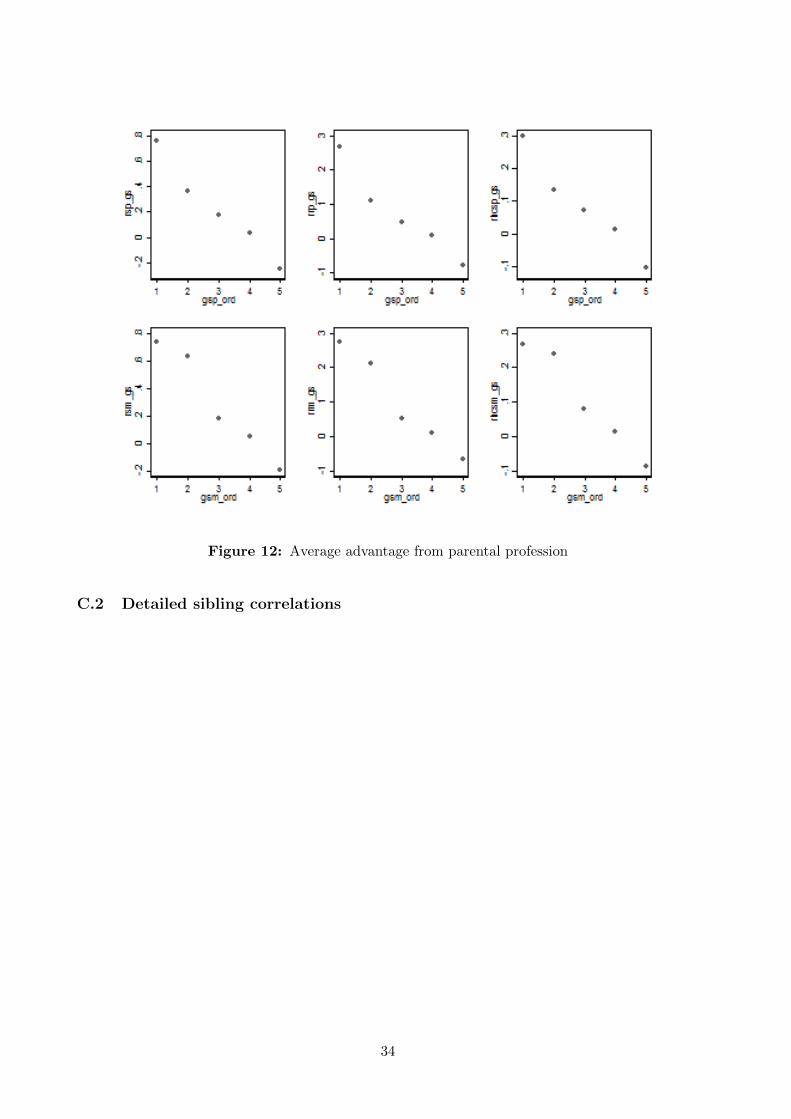
Figure 12: Average advantage from parental profession

C.2 Detailed sibling correlations

34

Tab

le16:

Sib

lin

gco

rrel

atio

ns

-by

gen

der

Ed

ucati

on

years

Pre

stig

esc

ore

An

nu

al

earn

ings

Non

-para

met

ric

4th

ord

erO

LS

15gr

oup

s30

grou

ps

OL

Sre

gres

sion

An

nu

alea

rnin

gs

gros

sn

etgro

ssn

etobs

.gr

oss

net

gros

sn

etobs

.gr

oss

net

gros

sn

etobs

.

All

0.5

780.

520

0.5

830.5

24

21

556

0.33

50.

342

0.33

00.3

37

19

673

0.41

00.

457

0.41

50.4

58

16

338

Bro

ther

s0.5

750.

534

0.5

820.

539

5157

0.35

80.

358

0.35

60.

355

4936

0.51

80.

516

0.51

80.

516

3896

Sis

ters

0.6

260.

555

0.6

290.

557

5434

0.38

70.

387

0.37

80.

378

4743

0.47

50.

467

0.47

80.

469

4234

Mix

edp

airs

0.5

530.

497

0.5

570.

501

10

965

0.31

10.

311

0.30

80.

307

9994

0.42

60.

426

0.42

70.

427

8208

p-v

alu

este

stin

gth

eeq

ual

ity

ofco

rrel

atio

nco

effici

ents

Bro

ther

s/S

iste

rs0.0

000.

120

0.0

000.

201

0.09

70.

096

0.20

10.

181

0.01

00.

003

0.01

60.

004

Bro

ther

s/M

ixed

0.0

470.

003

0.0

260.

002

0.00

20.

002

0.00

20.

002

0.00

00.

000

0.00

00.

000

Sis

ters

/Mix

ed0.0

000.

000

0.0

000.

000

0.00

00.

000

0.00

00.

000

0.00

10.

007

0.00

10.

006

Note

:N

um

ber

of

obse

rvati

ons

for

pre

stig

esc

ore

sco

rres

pond

toth

ecl

ass

ifica

tion

wit

h30

gro

ups,

the

one

counti

ng

only

15

gro

ups

yie

ldin

gsl

ightl

yhig

her

num

ber

s.

35

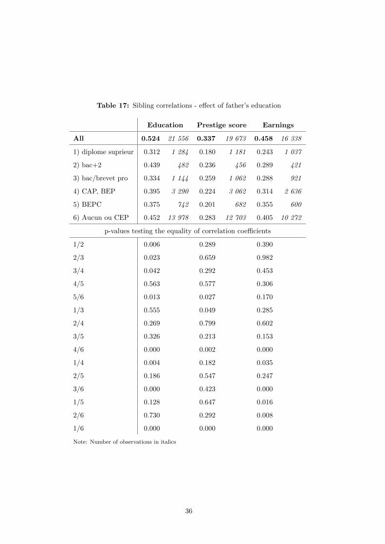
Table 17: Sibling correlations - effect of father’s education


All 0.524 21 556 0.337 19 673 0.458 16 338

1) diplome suprieur 0.312 1 284 0.180 1 181 0.243 1 037

2) bac+2 0.439 482 0.236 456 0.289 421

3) bac/brevet pro 0.334 1 144 0.259 1 062 0.288 921

4) CAP, BEP 0.395 3 290 0.224 3 062 0.314 2 636

5) BEPC 0.375 742 0.201 682 0.355 600

6) Aucun ou CEP 0.452 13 978 0.283 12 703 0.405 10 272


1/2 0.006 0.289 0.390

2/3 0.023 0.659 0.982

3/4 0.042 0.292 0.453

4/5 0.563 0.577 0.306

5/6 0.013 0.027 0.170

1/3 0.555 0.049 0.285

2/4 0.269 0.799 0.602

3/5 0.326 0.213 0.153

4/6 0.000 0.002 0.000

1/4 0.004 0.182 0.035

2/5 0.186 0.547 0.247

3/6 0.000 0.423 0.000

1/5 0.128 0.647 0.016

2/6 0.730 0.292 0.008

1/6 0.000 0.000 0.000


36

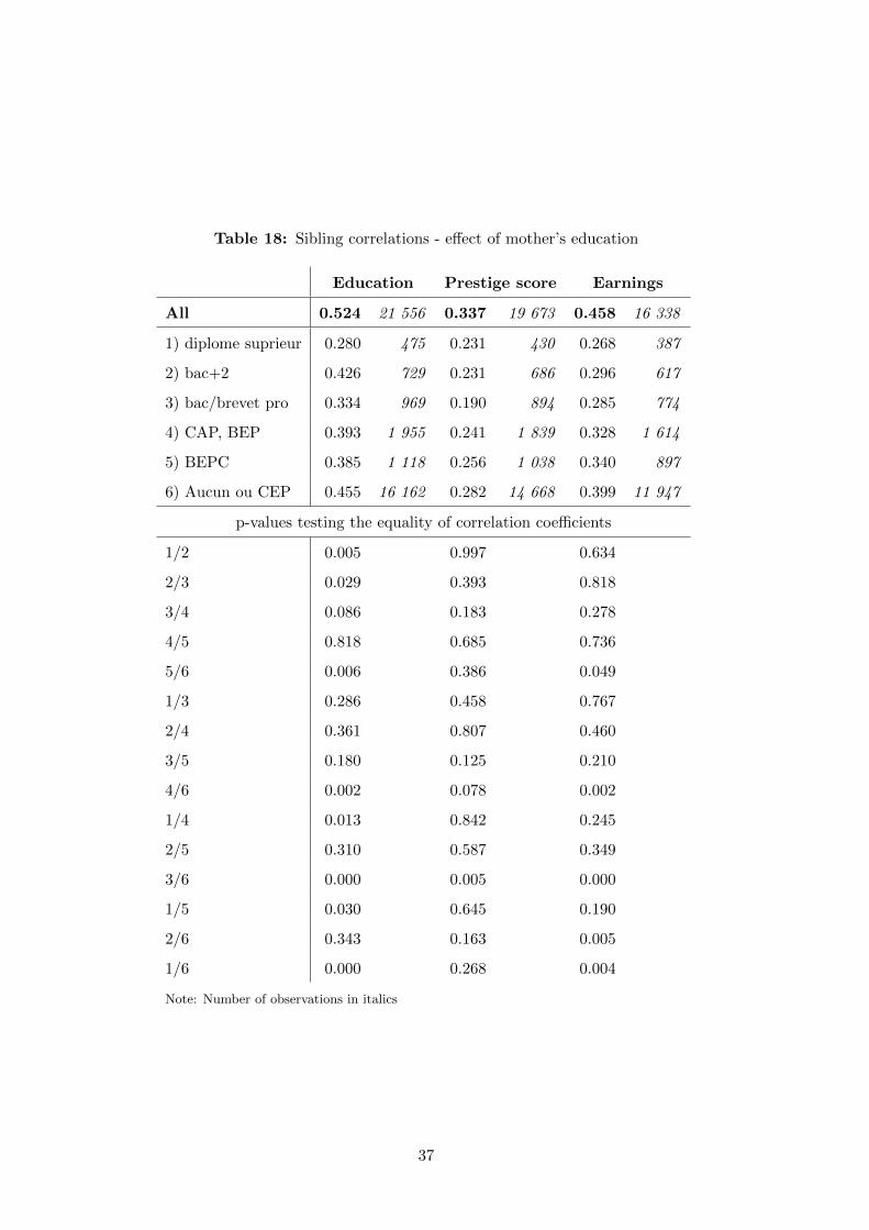
Table 18: Sibling correlations - effect of mother’s education


All 0.524 21 556 0.337 19 673 0.458 16 338

1) diplome suprieur 0.280 475 0.231 430 0.268 387

2) bac+2 0.426 729 0.231 686 0.296 617

3) bac/brevet pro 0.334 969 0.190 894 0.285 774

4) CAP, BEP 0.393 1 955 0.241 1 839 0.328 1 614

5) BEPC 0.385 1 118 0.256 1 038 0.340 897

6) Aucun ou CEP 0.455 16 162 0.282 14 668 0.399 11 947


1/2 0.005 0.997 0.634

2/3 0.029 0.393 0.818

3/4 0.086 0.183 0.278

4/5 0.818 0.685 0.736

5/6 0.006 0.386 0.049

1/3 0.286 0.458 0.767

2/4 0.361 0.807 0.460

3/5 0.180 0.125 0.210

4/6 0.002 0.078 0.002

1/4 0.013 0.842 0.245

2/5 0.310 0.587 0.349

3/6 0.000 0.005 0.000

1/5 0.030 0.645 0.190

2/6 0.343 0.163 0.005

1/6 0.000 0.268 0.004


37

Table 19: Sibling correlations - effect of father’s profession


All 0.524 21 556 0.337 19 673 0.458 16 338

1) farmer 0.435 2 553 0.217 2 368 0.383 1 362

2) skilled workman, ... 0.455 2 625 0.257 2 381 0.386 1 742

3) executive, ... 0.370 1 846 0.209 1 686 0.306 1 516

4) intermediate occupations 0.451 2 829 0.266 2 655 0.335 2 402

5) administrative, ... 0.444 2 277 0.277 2 089 0.383 1 886

6) laborer 0.419 8 694 0.256 7 881 0.364 6 905


1/2 0.368 0.145 0.926

2/3 0.001 0.111 0.010

3/4 0.001 0.053 0.316

4/5 0.749 0.689 0.077

5/6 0.200 0.362 0.407

1/3 0.011 0.792 0.019

2/4 0.847 0.736 0.065

3/5 0.005 0.028 0.011

4/6 0.070 0.632 0.166

1/4 0.468 0.067 0.108

2/5 0.619 0.480 0.914

3/6 0.023 0.065 0.021

1/5 0.708 0.034 0.995

2/6 0.046 0.958 0.348

1/6 0.389 0.079 0.463


38

Table 20: Sibling correlations - effect of mother’s profession


All 0.524 21 556 0.337 19 673 0.458 16 338

1) farmer 0.411 1 974 0.216 1 876 0.368 1 076

2) skilled workman, ... 0.420 1 326 0.226 1 220 0.380 887

3) executive, ... 0.375 292 0.230 260 0.231 231

4) intermediate occupations 0.446 1 723 0.245 1 606 0.348 1 442

5) administrative, ... 0.451 5 877 0.286 5 471 0.387 4 897

6) laborer 0.456 3 038 0.275 2 849 0.387 2 469


1/2 0.748 0.759 0.753

2/3 0.407 0.960 0.026

3/4 0.177 0.813 0.072

4/5 0.822 0.116 0.134

5/6 0.764 0.596 0.987

1/3 0.501 0.825 0.039

2/4 0.381 0.611 0.389

3/5 0.127 0.342 0.011

4/6 0.670 0.299 0.180

1/4 0.187 0.368 0.577

2/5 0.209 0.043 0.825

3/6 0.109 0.458 0.013

1/5 0.056 0.005 0.506

2/6 0.173 0.130 0.845

1/6 0.051 0.034 0.548


39

References

Bjorklund, A., T. Eriksson, M. Jantti, O. Raaum, and E. Osterbacka (2002): “Brother

Correlations in Earnings in Denmark, Finland, Norway and Sweden Compared to the United

States,” Journal of Population Economics, 15, 757–72.

Bjorklund, A. and M. Jantti (2009): “Intergenerational Income Mobility and the Role of

Family Background,” in Oxford Handbook of Economic Inequality, ed. by B. Salverda, W. Nolan

and T. Smeeding, Oxford: Oxford University Press, 491–521.

——— (2012): “How Important is Family Background for Labor-Economic Outcomes?” Labour

Economics, 19, 465–74.

Bjorklund, A., M. Jantti, and M. Lindquist (2009): “Family Background and Income During

the Rise of the Welfare State: Brother Correlations in Income for Swedish Men Born 1932-1968,”

Journal of Public Economics, 93, 671–80.

Bjorklund, A. and K. Salvanes (2010): “Education and Family Background: Mechanisms and

Policies,” IZA Discussion paper series, 5002.

Chambaz, C., E. Maurin, and C. Torelli (1998): “L’evaluation sociale des professions en

France. Construction et analyse d’une echelle des professions.” Revue francaise de sociologie, 39,

177–226.

Conley, D. and R. Glauber (2008): “All in the Family? Family Composition, Resources, and

Sibling Similarity in Socioeconomic Status,” Research in Social Stratification and Mobility, 26,

297–306.

Mazumder, B. (2008): “Sibling Similarities and Economic Inequality in the US,” Journal of

Population Economics, 21, 685–701.

——— (2011): “Family and Community Influences on Health and Socioeconomic Status: Sibling

Correlations Over the Life Course,” The B.E. Journal of Economic Analysis & Policy, 11.

Mazumder, B. and D. Levine (2004): “The Growing Importance of Family and Community: An

Analysis of Changes in the Sibling Correlation in Earnings,” Federeal Reserve Bank of Chicago

Working Paper, 24.

Schnitzlein, D. (2011): “How Important is the Family? Evidence From Sibling Correlations in

Permanent Earnings in the US, Germany and Denmark,” SOEP paper, 365.

40

Sibling correlations in terms of education, profession and ...

Documents

Transcript of Sibling correlations in terms of education, profession and ...