SHORTEST PAmS IN 3-SPACE, VORONOI DIAGRAMS WITH BARRmRS, AND RFLATED COMPLEllTY AND ALGEBRAIC ISSUES

Wm. Randolph Franklin and Varol Akman

Electrical, Computer, and Systems Engineering Department Rensselaer Polytechnic Institute Troy, New York 12180-3590, USA

Phone: (518) 266-6077, telex 646542

ABSTRACf

We consider the problem of computing the shortest path under the Euclidean metric between source and goal points in 3-space while avoiding clashes with polyhedral obstacles. This can be thought as the ultimate version of the notorious TRAVELING SALESMAN problem in terms of generality and is known as the FINDPAm problem in artificial intelligence and robotics. We show that this problem is solved using algebraic elimination techniques in a straightforward yet very inefficient manner. We then introduce a Voronoi-based strategy for solving the subproblem of determining the sequence of obstacle edges through which the shortest path passes. This is based upon a natural extension of Franklin's ''Partitioning the plane to calculate minimal paths to any goal around obstructions" [Tech. Rep., ECSE Dept., Rensselaer Polytechnic Inst., Troy, NY, Nov. 1982] to 3-space. In 3-space, a very desirable feature of the plane partitions disappears making the space partitions complicated. For this case, we suggest an approximation technique.

KEYWORDS: robotics, artificial intelligence, computational geometry, algebraic computing, TRAVELING SALESMAN problem, FINDPAm problem, Voronoi diagrams.

This material is based upon work supported by the National Science Foundation under grants ECS 80-21504 and ECS 83-51942. The second author is also supported in part by a Fulbright award.

NATO AS! Series, Vol. F17 Fundamental Algorithms for Computer Graphics Edited by R. A. Earnshaw © Springer-Verlag Berlin Heidelberg 1985

896

1. INTRODUCfION

Let P1 • Pa ••••• P be solid polyhedral objects in 3-space. A very important problemnin computational geometry (which is known as FINDPATH in artificial intelligence and robotics. and has wide applications) is to find a shortest path between two points Sand G (commonly termed as the source and the goal points) avoiding intersections with P .• i=l ••••• n. Touching the boundaries of P. is

1 1 allowed. Throughout this paper. we shall use the La (Euclidean) metric to measure distances.

In 2-space where the obstacles are polygons whose interiors are forbidden. the problem is easy to solve. Since the shortest path can only be a polygonal path whose vertices bend at the vertices of the given polygons the problem is reduced to the following subproblems: (1) Construct a "visibility graph" whose nodes consist of {S.G} U {T: T is a vertex of P .• i=l ••••• n}. A link in this

1 graph connects a pair of vertices visible from each other and carries a weight equal to the distance between these vertices. (ii) Search through this graph to find the shortest path from S to G using an algorithm such as Dijkstra [1959]. Lee-Preparata [1984] mentions an algorithm to accomplish steps (i) and (ii) in O(ma log m) total time where IFl:.lp.l. (ipi denotes the n11lDber of vertices of polygon P.) 1 1

In 3-space the problem is much more difficult. In this case. the shortest path is al so a polygonal path but the only thing we can say about its vertices is that they bend on the edges of the given polyhedra. The characterization of these bend points is a formidable task.

There have been various developments in the area of path planning in the last two decades. For brevity. we shall mention only a certain section of it. (Akman [1984] contains a long list of references.) Lozano-Perez [1981. 1983]. Brooks [1983]. Donald [1983]. and Nguyen [1984] report many applications oriented toward robotiCS. Reif [1979]. Schwartz-Sharir [1983a. 1983b. 1983c. 1984]. Sharir-Arielsheffi [1984]. Hopcroft-Schwartz-Sharir [1984]. O'Ounlaing-Yap [1983]. Spirakis-Yap [1983. 1984]. and O'Ounlaing-Sharir-Yap [1983] report work mostly on the computational complexity of several special cases of path planning. Finally. shortest path computation has also been treated in recent papers such as Franklin [1982]. Franklin-Akman [1984]. Franklin-Akman-Verrilli [1985]. Sharir-Schorr [1984]. Lee-Preparata [1984]. and O'Rourke-Suri-Booth [1984]. Sharir and Schorr's work is especially interesting in that it mentions many results on the nature of shortest paths on a convex polyhedron. For example. they prove that "A shortest path cannot pass through a vertex or a ridge point of the polyhedron" where a ridge point is defined as a goal point on the polyhedron for which there are at

897

least two shortest paths from a given S on the polyhedron. The crux of their paper nevertheless is the following result which is arrived after employing complex data structures and algorithms:

"Given a convex polyhedron P and a point S on it, P can be preprocessed in O(lpl' log Ipl) time to produce a data structure (taking O(lpl') space) with the help of which one can find in O(lpl) time the shortest path along the surface of P from S to any G."

The shortest path problem is in some ways may be considered as an extension of the NP-complete (in the strong sense) TRAVELING SALESMAN problem (TSP) where we wish to determine the shortest path (or tour) that traverses the nodes of a given graph in any order, cf. 10hnson-Papadimitriou [19811 and Papadimitriou-Steiglitz [19821. Although there are some technical difficulties arising from the distance metric, the Euclidean version of TSP (ATSP) is also NP-complete as shown by Papadimitriou [19771.

Rest of this paper is organized as follows. Section 2 treats the problem of finding the shortest paths in 3-space using an algebraic approach. Section 3 deals with the subproblem of specifying which sequence of edges a shortest path should follow. Finally, Section 4 mentions some complexity issues and algebraic problems created by shortest path determination.

2. SHORTEST PATHS IN 3-SPACE: AN ALGEBRAIC APPROAm

If we want to find the shortest path from S to G in the presence of obstacles P., i=l, ••• ,n, the first thing is to check

1 whether G can be reached from S directly. Note that, since we allow a shortest path to touch an obstacle, this would entail checking line segment SG against each P. for at most one intersection. This can be done USing standard metiods. Chazelle-Dobkin [19791 gives a fast (O(log' Ipl» algorithm for line-polyhedron intersection detection for convex polyhedra. Thus, in the sequel, we shall assume that such a check has already been made and SG is not the shortest pa tho

It is intuitively clear that the shortest path from S to G will be a polygonal path which bends on some edges of some obstacles, i.e., it cannot touch the interior of a face of an obstacle. (A formal proof is quite involved; Chein-Steinberg [19831 gives a proof in 2-space.) This observation immediately gives an algorithm to compute the shortest path. First, list all permutations of {e: e is an edge of P., i=I, ••• ,n} of positive length. Second, for each

1 permutation in this list, compute the shortest of the polygonal paths which visits each line of this permutation exactly once in the

898

given order. Thus. at the end of this step. we have a list of permutations and the shortest polygonal paths associated with each permutation. (A polygonal path is specified by its consecutive vertices: S. bend pOints on the lines belonging to a permutation in that order. and G.) Now start at the top of this list. Test the shortest polygonal path associated with this permutation against each Pi for intersection. The only intersection points reported by this process must be the ones that we already know. i.e •• the vertices of the polygonal path at hand. Otherwise. we discard this polygonal path (because it passes through one or more obstacle(s» and continue with the next permutation. We note in passing that in Sharir-Schorr [1984] this last step is missing; thus their algorithm is incomplete.

It is emphasized that when there are more than one shortest paths. with a slight modification of the above algorithm one can obtain all of them. The number of shortest paths is an interesting problem in itself. Figure 1 shows a particular arrangement of a workspace in 2-space which clearly demonstrates that there may be an exponential number of shortest paths between Sand G. A few things need some explanation in this figure. It is assumed that Pand all the even-numbered obstacles are semi-infinite or large enough so that a sJtortest path cannot tour around them. All P .• i=l ••••• n.

1 and the "teeth" of P are aligned along the line connecting S to G. In this specific case there exist 20 •Sn shortest paths. It is trivial to extend this workspace to 3-space by simply erecting prisms for each polygon.

Given a permutation. the problem of finding the bend points of a shortest polygonal path on these lines can be solved using algebraic means. Before we proceed to show this. we shall state a problem and two useful lemmas regarding shortest polygonal paths through a set of lines. (For proofs of the lemmas. cf. Sharir-Schorr [1984].)

LINE VISITATION problem (LVP): Given a sequence 11 .13 ••••• 1 of lines in 3-space. what is the shortest path from S to G n constrained to pass through each of the lines 11 , 13 ••••• 1 in this order? n

Let C1 • C3 ••••• Cn be the bend points of the shortest path on the given lines. For notational ease. we shall denote S (resp. G) by Co (resp. Cn+1).

LEMMA 2.1. For each i=l ••••• n. the angle between Ci - 1Ci and Ii is equal to tJte angle between C.C. 1 and 1 .•

1 1+ 1

LEMMA 2.2. The shortest path from S to G passing through the sequence of lines 11 , 13 ••••• In in this order is unique.

We now give some allebraic prel iminaries that w ill be nece ssary

899

for the upcoming presentation. Let A and B be polynomials of positive degree with coetficients in a commutative ring with an identity element. If A(x)=Laixi and B(x)=lbixi where degree(A)=m and degree(B)=n, the "Sylvester matrix" of A and B is the m+n by m+n matrix:

a m

b n

a m-l

a m

b n-l

b n

a m-l

a m

b n-l

b n

a o

a m-l

b 0

b n-l

a o

b 0

a 0

b o

in which there are n rows of A coefficients, m rows of B coefficients, and all elements not printed are O. The "resultant" of A and B, denoted by resul tant (A, B), is the determinant of the Sylvester matrix.

THEOREM 2.1 (Collins [1971]). If A and B are polynomials of positive degrees over a unique factorization domain then resul tant (A, B) =0 if and only if A and B have a common div isor of positive degree.

In this paper, we shall be dealing with multivariate polynomials. In this case, the following interpretation of the resul tant becomes crucial. The resul tant of two mul tivariate polynomials A and B (both liven in variables x1 ' xa, ••• , xr ) with respect to xs ' 1isir is obtained as follows: (i) Write both A and B in terms of sinlle variable x treatinl the other variables as s constant s. (ii) Compute the resul tant of these new polynomial s usinl the orilinal definition above. The outcome of this is another polynomial with one less variable, i.e., x has been eliminated. We shall denote it by resul tant (A, B, x ). s

s

THEOREM 2.2 (Collins [1971]). Let A and B be multivariate polynomials in variables x1 ' xa , ••• , x with positive degrees m and r n respectively. Write both A and B in terms of the sinlle variable xr as explained above. Let C be resultant(A,B,xr ). If (a 1 ,aa, ••• ,ar ) is a common zero of A and B then C(a1 ,aa, ••• ,ar-l)-0.

900

Conversely. if C(a1 .a" ••••• ar-1)=0. then at least one of the following is true:

(a) All coefficients of A are O. (b) All coefficients of Bare O. (c) The constant coefficients of A and B are both O. (d) For some a r • (a1 .a" ••••• ar ) is a common zero of A and B.

This theorem immediately suggests a way to solve multivariate polynomial equations simultaneously.

EXAMPLE 2.1 (adapted from Collins [1971). Let [A=O.B=O.C=O) be a system of three equations in variables x.y.z with integer coetficients. Compute f (x )=resul tant (resul tant (A. C. z) • resul tant (B. C. z) .y). By Theorem 2.2. if (a.b.c) is a solution to the given system then f(a)=O. SimilarlY we can compute polynomials g (y) =resul tant (resul tant (A. C. z) • resul tant (B. C. z) • x) and h(z)=resultant(resultant(A.C.y).resultant(B.C.y).x) such that g(b)=O and h(c)=O whenever (a.b.c) is a zero of the system. Thus. one can solve f. g. and h individually to find their roots to arbitrary accuracy and then decide which triples (a.b.c) are solutions of the system.

Now we proceed to outline the algebraic solution to the LVP. In the following we refer the reader to Figure 2. Assume that each line is given by its two distinct points and assign different coordina te systems to each 1 ine. i. e •• let 1 ine 1. be parametrized

1 by Xi. Also. for each line compute Ni which is a unit vector along Ii in any direction. (IIVII denotes the length of vector V.) From Lemma 2.1. it is seen that:

C. 1C .• N. C.C.+1 .N. 1- 1 1 1 1 1 ----------=----------

If we rewrite the above equation after inserting values of Ci - 1 • Ci • Ci +1 in terms of Xi-I' Xi' xi+1' respectively. and remove the square root signs. then we obtain a quartic in three variables. Xi-I' Xi' and xi +1 • Repeating this for all lines. we end up with the following system of n quartics:

Q1(X1' X,,)=0 Q" (X1' X" .X, )=0

Qi(Xi - 1 ·Xi ·xi +1)=0

Qn(xn-1, xn)=0

Theoretically. the above system of equations can be solved

901

using resultants as demonstrated in Example 2.1. This is a classical method known as the "elimination theory", cf. Van der Waerden [1970]. Alternatively, we can use a numerical technique such as the Newton-Raphson method for solving a system of nonlinear equations.

If 11 , la, ••• , In are but line segments then the shortest path may be bending at points located outside these line segments. In this case, Sharir-Schorr [1984] states that the shortest path will have to pass through some endpoints of these segments at which it will subtend different entry and exit angles contrary to Lemma 2.1. Thus the problem is reduced to a collection of subproblems where a shortest path passes through the interior points of a subsequence of 1 ine se gment s.

3. PARTITIONING 3-SPACE AROUND POLYHEDRA

A common specialization of the shortest path problem occurs when S and the obstacles are fixed, and new paths should be calculated as G moves around the workspace. For example, a manipulator arm may pick up a part from a pile of parts in a fixed locahon, and then move somewhere in the scene to work with it.

In Frankl in [1982], an important construction based on an extension of Voronoi diagrams in the plane is given which, for a given S in 2-space, partitions the plane into a set of regions such that all the G within any given region have the same list of bend pOints. (For another extension of Voronoi diagrams, see Lee-Drysdale [1981].) This reduces the problem of finding a shortest path to the preprocessing step (finding the regions), plus the task of determining which region contains G (searching or querying). The last step is easy since the borders of the regions are either straight line segments or portions of hyperbolae. Thus, existing pOint location algorithms can be used after some slight modifications. In the common case where G varies while S and the obstacles are fixed, the shortest path can be found by merely repeating the search (point location) phase.

In this section, we shall try to emulate Franklin's approach in 3-space. Here, the regions will have the following property: All the points in a given region are reached from S after visiting the same sequence of edges of the obstacles. We first work on a very simple case, namely, a sol id triangle.

Let W1 , Wa' and W, be points in 3-space. These points describe a triangle W1WaW. if they are not colinear. Let S be any point in 3-space not in the plane E of W1WaW •• Assuming that W1WaW. is a solid triangle we want to partition the space into regions such that

902

if a DeW point G is specified we would be able to tell whether G can be directly reached from S. and if not. which edge of the triangle (W1Wa• WaW •• or W, W1) the shortest path must touch.

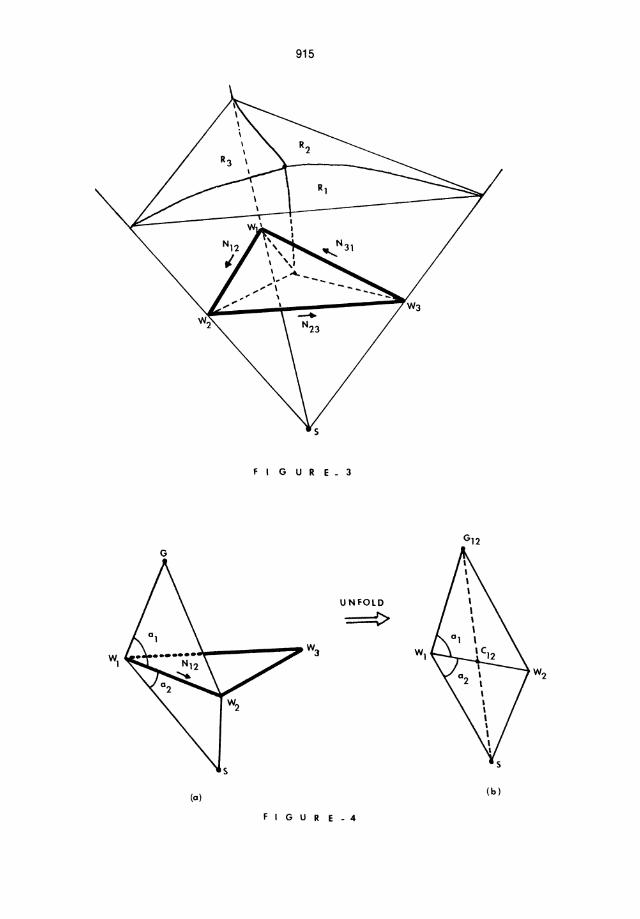
Obviously. if G is outside the semi-infinite prism (frustum) obtained by subtracting the pyramid described by base W1 WaW• and apex S from the infinite pyramid described similarly then the shortest path is SG. Thus we found one of the regions. Ro. Note

that Ro has all the points of the space that are not obstructed by W1WaW •• See Figure 3.

Otherwise. G may belong to one of three regions R1 • Ra. or R ••

~ is the region such that if GaR1 then the shortest path is via edge WaW •• Ra is the region such that if GaR a then the shortest path is via edge W,W1. Finally. R, is the region such that if GaR. then the shortest path is via edge W1Wa • When G is on the boundary of two regions there may be two or three shortest paths.

Now. we shall compute the boundaries between the pairs R1 and Ra. Ra and R, • and R, and R1 • In the sequel. S is assumed to be the origin. (This is easy to achieve by translating everything in the wortspace by -S.) We shall first compute the boundary between R1 and R, • Tate G such that SG n W1WaW. is not empty. If GaR1 n R. then there exists a path to G either via W1Wa or via WaW. and rendering equal lengths. Labeling the bend points of these paths with the triangle by Cl2 and C23 • we get:

SCI2+CI20=SC23+C23G

The left hand-side is equal to IIG12 11 where G12 is the point obtained by rotating G about W1 Wa until it is coincident to the plaDe of SW1Wa and on the opposite side of S with respect to W1 Wa • Similarly. the right hand-side is equal to IIG23 11 where GZ3 is the rotated image of G about WaW,.

Before we continue with our analysis. we give a list of useful vector and trigonometric identities that we shall employ frequently. (x and. denote vector cross and dot products.)

(ll) IIAlla=1 if A is a unit vector. (IZ) Ax(BxC)=(A.C)B-(A.B)C (13) (AXB).(CxD)=1 A.C A.D I=(A.C)(B.D)-(A.D)(B.C)

B. C B.D (14) IIA+Blla=IIAlla+IIBllall+zIIAIl IIBIlcos a

where a is the angle between A and B. (IS) sin Ze=Zsin acos a (16) cOll(a+o)=cos acos O-sin asin 0

It is bown that if P is a point and P' is its rotated version by an angle e about an axis U (a unit length vector) passing through the origin then:

903

P'=(P.U)U+(P-(P.U)U)cos 9+(UxP)sin 9

Using the last formula, it is easy to see that:

G12=W1 +fN12+(W1 «r-fN12)co s u+(N12xW1 G) sin u

where u is the dihedral angle between the planes of triangles SW11S and GW1 Is, N12=W1 I s/lIw 1 I sii. and f=W1 G. N12 • Using (IS):

II G12 ll s = (a) (11 +fN, 2)2 (b) +(W1«r-d~'12)ScosS u (c) +(N xl1G)2sinS u (d) +2(~+fN12) • (W1«r-fN12)cos u (e) +2 (W1 +fN.12) .(N 2xW1G)sin u (f) +(W1 «r-fN12) • (N!2xI1Ghin 2u

The following are the simplifications:

Using (11), (a) is simplified to IIW1I1s+2f(W1.N12)+fS.

(b) is simplified to (1IW1Glls-fS)cos S u.

Using (13), (c) is simplified to (IIW1Glls-fS)sinS u.

Using (11), (d) becomes 2(W1 .11 «r-f(W1 .N12) )cos u.

(e) is simplified to 2(W1 .(N12xW1G». (f) is identically O.

It is possible to simplify (d) and (e) further. Noting that the normal of the plane of the triangle SW1,s is:

and the normal of the plane of the triangle GW1 Is is:

one obtains:

After some routine calculations, one arrives at:

W 1. (W1 «r- fN12) cos u=----------------------

I IN12x11 1 1 I IW1 GxN12 I 1

In a similar manner, but using the cross product:

904

sin

sin

a=IIMS12xMG1211, or equivalently

I IW1 .(N12xW1G) I I a=----------------------

IIN12xW1 11 IIW1 GxN12 I I

Thus, we showed that:

2cos a(W1 • (W1 G-fN12»= 2cos~ allN12xW1 11 IIN12xW1 GII and

2sin a(W1 .(N12xW1G»= 2 sin~ al IN12xw1 1 I IIN12xW1 Gil

Returning to our original equation, we obtain a more symmetric equa hon:

Now, we shall give a geometric interpretation of this equation. Expanding the dot and cross products in (*), we obtain:

IIG1211~=IIW 11~+IIW1GII~ +2(ltw1Gllcos a11IW11Icos(n-a~) +IIW1 Gllsin a 1 11W1 11 sin(n-a~», or

IIG12II~=IIW111~+IIW1GII~ -211W1 GII IIW1I1cos(a1+a~), using (16).

Above, a1 and a~ are the angles of GW1W~ and SW1W~, cf. Figure 4a. Finally, it is emphasized that this last formula is simply a statement of (14) on triangle SW1 G12 as can be seen from Figure 4b.

Up to this pOint, we found a formula which gives IIG1211~ in

terms of known quantities (W1 and N12) and the unknown G (with

coordinates x,y,z). The formula for IIG2311~ (resp. IIG31I1~) is

analogous to (*); just change W1 to W~ (resp. WI) and N12 to N23 (resp. N31 ). In terms of degree, the following example shows that

the surfaces between regions R. are in general ternary quartics 1

a1 though they may de genera te to pI ane s in some ca se s.

EXAMPLE 3.1. Given the triangle with coordinates W1 (1,2,1), W~(O,O,1), and W,(2,O,1), we shall compute the boundaries of regions R1 and R~, R~ and R" and RJ and R1 •

Using (*), the surface between regions R1 and R~ is found as

IIG12II~-IIG2311~=O, or:

905

-2x-4y+l0+2(x+2y-S + J(z-I)2+(I/S) (2x-y) 2_ V(z-I)3+y2)=0

which is further simplified to:

(2x-y)2=Sy2

The surface between R2 and R, is given by 11623112-11631112=0. or:

4x-8+2(-(2/S) (x-2y-2) + v(z-I)2+y2- V~(~21~/~S~)~(-z--I~)~2~+~(~2~1~/2~S~)~(~2-x-+y---4~)~2)=0

or. after some operations to remove the square root signs:

2S6z4 -1024z'+(228y2+(2S6-128x)y-128x 2+S12x+l024)z2 +(-4S6y2+(2S6x-SI2)y+2S6x 2-1024x)z-48y4

+(S76-288)y'+(-272x 2+1088x-860)y2 +(32x'-192x 2+2S6x)y+16x 4-128x J +2S6x 2=0

Finally. the surface between R, and R1 is found to be:

which is also transformed to a quartic omitted here for brevity.

THEOREM 3.1. Let P be a convex polygon with vertices V1 • V2 ••••• Vn and 8 a point outside the plane of P. It is possible to partition P into at most n convex regions (each completely containing an edge of P) such that if 6 is later specified inside one of these regions then the shortest path between 8 and 6 is via the associated edge of this region.

Prool. We give a constructive proof. Rotate 8 about the lines defined by edges V1V2• V2V" etc. until it is coincident to the plane of P and always on the opposite side of a particular edge compared to the interior of P. This is basically an unfolding of the pyramid with apex 8 and base P to the base plane. Thus. n image points are obtained which will be denoted by 812 , 823 , etc. Draw the Voronoi diagram of these points and clip it against the window P. This partitions P into at most n convex regions since each Voronoi polygon is convex. Figure S demonstrates this operation. Let us denote the regions by ~2' ~3' etc. It is seen that there is a border line passing through each vertex of P. It is obvious that if 6 is inside a region R .. then we just connect it to the

1J associated image point of this region. namely 8 ..• The intersection of this line segment with the associated edge V~. of this region is

1 J the bend pOint X of the shortest path from S to 6. X may be placed into 3-space by folding again.

Theorem 3.1 hints an important property of the regions R1 • R2• R,. namely. their intersections with the plane of '1W2W, must be

906

straight lines. Returning to Example 3.1:

EXAMPLE 3.1 (continued). To see the intersection of the boundary between R1 and R~ with E (the plane of the triangle) put z=1 in their boundary equation. This gives:

2 y=-----x

1+E

Continuing with the boundary of R~ and R, we obtain the line:

-( 8+2 .J21h:+16+4 v'2i y=--------------------

9+ V2i

Finally. for the boundary of R, and R1 • we have:

(8+2 V21+2 /S)x-16-4 V21 y=----------------------

-4+ vs- Vfi

These three lines intersect at:

16+4 ill X=( {S+1)Y/2. Y=----------------

13+2 ill+4 .JS+ 11'105

in the z=1 plane. Point (X.Y) has the property that it is possible to go from S (origin) to (X.Y) on a shortest path touching any edge of W1W~Wa. Furthermore. it is the only such point on E. As a final note. (X.Y) can also be obtained as the intersection of the three Voronoi polygons constructed by the images of S on E as described in Theorem 3.1.

It is emphasized that the method exemplified up to now can be applied in the presence of a solid polygon too. In this case we are required to compute all the potential boundaries between pairs of regions. Although conceptually easy. this would be a difficult when it comes to intersect boundaries to compute their intersection curves.

The extension of the method to more than one obstacle (polygon) seems difficult. In this case. a very desirable property of plane parti tions around polygons as discovered by Frankl in disappears. We shaH depict this with the aid of Figure 6a. First. a brief account of Franklin's approach is in order. (The reader is referred to Franklin [1982] and Franllin-Akman-Verrilli [1985] for a detailed description.) Note that in the plane. once a subdivision is formed there is only one sequence of bend points for it (provided that it is not on a boundary curve in which case there may be more). In

907

Figure 6a, there are two obstacles (line segments) A1B1 and AzB z in

the plane and a source S is given as shown. Frankl in's algorithm parti tions the pI ane into 5 regions in this ca se. Ro hoI ds goal points directly reachable from S. ~ holds points which cause a shortest path to bend at B1 • Rz holds points which cause a shortest path to bend at A1 • The boundary between R1 and Rz is a portion of a hyperbola. R. holds pOints which give rise to a shortest path bending at Bz • Finally, R. describes shortest paths bending first at A1 and then at Az • The boundary of R, and R. is also a portion of a hyperbola. All other boundary curves are linear. A crucial property of this diagram is as follows: "A bend point acts as a source point for a later region." For instance, ~ acts as a souce point for the points of R •• Similarly, B1 acts as a source for the points of R,. Thus, the source point is continuosly "pushed back" and this is the underlying reason for the fact that all curves are ei ther 1 ine segments or hyperbol ic sections.

In 3-space, we cannot immediately see an analogue of this property. When we place another triangle V1VZV. in Example 3.1, the new regions induced by this obstacle will be separated by surfaces of order higher than four (Figure 6b). Thus, whereas the boundary curves remain as hyperbolae in 2-space, in 3-space they would grow with every new polygonal obstacle placed into the workspace. One practical way to get around this problem is to approximate the boundaries with more manageable surfaces (such as quadrics) and to keep them as such even when new obstacles are introduced. This, we thinK, is possible since the boundary surfaces are generally smooth. The reader is referred to Figure 7 where we plotted the intersection curves of the boundaries computed in Example 3.1 with the z=2 plane.

4. OOMPLEXITY AND ALGmRAIC ISSUES

The method outl ined in Section 2 to find the shortest paths is a brute force approach. However, this may be the only available approach in the light of striking similarities of our problem and the TSP. It would be interesting to determine whether there is a heuri stic for this probl em 1 ike Chri stof ide s' 50-percent heuristic for TSP (Garey-Johnson [1979]). We now give a partial complexity analysis for Section 2.

The enumeration of the permutations of positive length as required by the algorithm takes time proportional to the factorial of the total number of edge s of the given polyhedra. Given a permutation, finding the bend points using resultants is also a costly process. If A and B are polynomials in variables x1 ' xa, ••• ,xr and C=resultant(A,B,xr ) then C is the sum of at most

(mr+nr)! terms, each of which being a product of nr A coefficients

and mr B coet"ficients. (A and B have degrees mr and nr in variable

908

xr .) It can be shown that the degree of C in variable xr - 1 is

bounded above by mrnr-1+nrmr-1 if A and B have degrees mr-1 and nr - 1 in xr71 • Therefore, 2M N is seen to be an upper bound on the degree of C If M=max. m. and N=max. n .•

1 1 1 1

In Collins [1971], the computing time of a resultant algorithm is analyzed as a function of the degrees and the coefficient sizes of its input s. As a special case it is proved that when all degrees are equal and the coefficient size is fixed, the computing time is O(dcr ) where d is the common degree, r is the number of variables, and c is a constant.

It can be seen that the detection of the intersections of a polygonal path with the obstacles as required by our algorithm will be subsumed by the previous computations. The following is a crude argument when all P. are convex. Take a polygonal path made of k line segments. Tesling this against all polyhedra takes O(n:& v log:& v) time in the worst case of k=O(n v) where v=max.lp.l.

1 1

There are technical problems with the Euclidean FINDPATH as stated by Papadimitriou [1977] and Garey-Graham-Johnson [1976] in the context of ATSP. It is known that (Grunbaum [1967J and Franklin [1983]) there exist configurations in the real projective plane which are not realizable in the rational projective plane. In the light of this, we must require infinite precision in the input (polyhedral vertex coordinates), i.e., a symbolic rather than numeric approach in inputting the coordinates. Even when one imposes the restriction that only points with rational coordinates be allowed as input, it is easy to end up with irrational distances under the Lz metric. This can be deal t with as long as one keeps such distances merely as square roots and employs algebraic manipulation algorithms. However, if we state FINDPATH as a decision problem, i.e., ''Does there exist a shortest path with length A or less?H we suspect that FINDPATH becomes NP-complete. This originates from the difficulty of comparing numbers symbolically, or in other words, the identification of algebraic numbers (Mignotte [1982). The symbolic expression for the length of a given shortest path on n lines may involve n+l square roots. An attempt to compare this expression to an integer l by repeated squaring to el imina te the square roots can take exponential time. An alternate way would be to evaluate each square root with sufficient accuracy so that their sum can be compared to l. There is a best-known upper bound on the number of operations required to achieve that, namely, O(m 2n), cf. Garey-Graham-Johnson [1976]. Here m is the number of digits with guaranteed correctness. Unfortunately, there is no known polynomial way to reach this accuracy.

The drawbacks that we mentioned can be avoided if we replace the Euclidean metric by another which closely approximates it. Define d'(x,y)=rd(x,y>l using the regular ceiling function. It is

909

trivial to show that this still is a metric satisfying the triangle inequality. The loss of precision can be tolerated if in the beginning everything is scaled by an appropriately large number.

Regarding the Voronoi approach outlined in Section 3, there are many unanswered questions. To our best knowledge, point location in 3-space in the presence of curved surfaces of arbitrary complexity is an area with not many results. Kalay [1982] considers point location in the presence of polyhedra. Recent work reported in Chazelle [1983], drawing inspiration from a method published by Arnon-COllins-Mccallum [1984a, 1984b] is at least conceptually applicable to our problem. In general, Chazelle proves that given n fixed-degree r-variate polynomials with rational coefficients, after O(nc(r» preprocessing time and spending polynomial space, it is possible to determine the region including a given point in O(2 r log n) time. (Note, however, that c(r) is an exponential function of r.) In fact, the mentioned work of Arnon-COllins-Mccallum has many other far-reaching applications in algebraic geometry, one of them being the problem of intersecting high-order surfaces as required by our Voronoi approach in Section 3.

910

REFERENlES

V. AlMAN, Findminpath algorithms for task-level (model-based) robot programming, Tech. Rep., ECSE Dept., Rensselaer Polytechnic Inst., Troy, NY, March 1984.

D. ARNON, G. E. COLLINS AND S. MCCALLUM, CYlindrical algebraic decomposition I: the basic alsorithm, SIAM Journal on Qomputing 13, 4 (Nov. 1984),865-877.

D. ARNON, G. E. COLLINS AND S. MCCALLUM, CYlindrical algebraic decomposition II: an adjacency algorithm for the plane, SIAM Journal on Qomputing 13, 4 (Nov. 1984). 878-889.

R. A. BROOKS, Solving the Find-Path problem by good representation of free space, IEEE Transactions on systems. Man. and Cybernetics 13, 3 (March/April 1983). 190-197.

B. M. CBAZELLE, Fast searchins in a real algebraic manifold with applications to geometric complexity, Tech. Rep., Computer Science Dept., BrownUniv., Providence. RI, June 1984.

B. M. CBAZELLE AND D. DOBKIN, Detection is easier than computation, Proc. 12th ACM SIGAcr Conf. (May 1979), 146-153.

O. CBEIN AND L. STEINBERG, Routing past unions of disjoint linear barriers, Networks 13 (1983),389-398.

G. E. COLLINS, The calculation of multivariate polynomial reaul tant s, Journal of the ACM 18, 4 (Oct. 1971), 515-532.

E. W. DIJKSTRA, A note on two problems in connexion with graphs, Numerische Mathematik 1 (1959), 1, 269-271.

B. R. DONALD, The Mover's problem in automated structural design, Tech. Rep., Artificial Intelligence Lab, Massachusetts Inst. of Technology, Cambridge, MA, June 1983.

W. R. FRANKLIN, Partitioning the plane to calculate minimal paths to aD¥ loal around obstructions, Tech. Rep., ECSE Dept., Rensselaer Polytechnic Inst., Troy, NY, Nov. 1982.

W. R. FRANKLIN AND V. AlMAN, Minimal paths between source and

911

soal points located on/around a convex polyhedron, Proc. 22nd Allerton Conf. on Communication. Control. and Computing (Sep. 1984).

W. R. FRANKLIN, V. ADfAN AND C. VERRlLLI, Voronoi diasrams with barriers and on polyhedra for minimal path planning, The Visual Computer - An Interna tional Journal on Computer Graphics (1985).

W. R. FRANKLIN, Alsebra problems in CAD com put a tions, Tech. Rep., ECSE Dept., Rensselaer Polytechnic Inst., Troy, NY, Oct. 1983.

)1. R. GAREY, R. L. GRAHAM AND D. JOHNSm, SOllIe NP-complete geOllletric problems, Proc. 8th ACII Symp. on Theory of Computing (May 1976),10-22.

M. R. GAREY AND D. S. JOHNSm, Computers and Intractabil ity: A Guide to the Theory of NP-completeness, Freeman, San Francisco, CA, 1979.

B. GRUNBADM, Copyex Polytopes, Wiley, New York, 1967.

J. E. HOPCROFl', J. T. SCHWARTZ AND II. SHARIR, On the complexity of motion plannins for mul tiple independent obj ect s; PSPACE hardness of the ''Warehouseman's problem", Tech. Rep., Computer Science Div., New York Univ., Courant Inst. of Mathematical Sciences, New York, Feb. 1984.

D. S. JOHNSm AND C. H. PAPADIMITRIOU, Computational complexity and the Travelins Salesman problem, Chap. 3 of The Trayeling Salesman Problem, eds. E. L. Lawler, J. K. Lenstra and A. G. Rinooy Kan, Wil ey, New York, 1981.

Y. E. KALAY, Determinins the spatial containment of a point in general polyhedra, Computer Graphics and Image Processina 19 (1982), 303-334.

D. T. LEE AND R. L. DRYSDALE, Generalizations of Voronoi diasrams in the plane, SIAM Journal on Computing 10, 1 (Feb. 1981), 73-87.

D. T. LEE AND F. P. PREPAlATA, Euclidean shortest paths in the presence of rectil inear barriers, Networks 14 (1984), 393-410.

T. LOZANO-PEREZ, Automatic planning of manipulator transfer movements, mEE Transactions on Systems. Man. and Cybernetics II, 10 (Oct. 1981), 681-698.

912

T. LCllANlrPBREZ, Spatial planning: a Configuration Space approach, IEEE Transactions on Computers 32, 2 (Feb. 1983), 108-120.

M. MIG NOTTE, Identification of algebraic numbers, lournal of Algorithms 3 (1982), 197-204.

V-D. tlHJ1EN, The Find-Pa th probl em in the plane, Tech. Rep., Artificial Intelligence Lab, Massachusetts Inst. of Technology, Cambridge, Mass., Feb. 1984.

C. 0' DUN..AING, M. SHARIR AND C. K. YAP, Retraction: a new approach to motion-planning, Proc. 15th ACM Symp. on Theory of Computing (April 1983), 207-220.

C. O'DUN..AING AND C. K. YAP, The Voronoi method for motion-planning: I. The case of a disc, Tech. Rep., Computer Science Div., Now YorkUniv., Courant Inst. of Mathematical Scienoes, Now York, March 1983.

1. 0' lOURIE, S. SURI AND H. BOO'lB, Shortest pa ths on polyhedral surfaces, Proo. 2nd Annual Symp. on Theoretical Aspect s of Computer Science (Ian. 1985).

C. H. PAPADIMITRIOU, The Euclidean Traveling Salesman problem is NP-complete, Theoretical Computer Science 4 (1977), 237-244.

C. H. PAPADHIITRIOU AND K. STEIGLITZ, Combina todal Optimization: Algorithms and Complexity, Addison-Wesley, Reading, MA, 1982.

1. H. REIF, Complexity of the Mover's problem and generalizations, Proc. 20th IEEE Conf. on Foundations of Computer Science (1979),421-427.

1. T. SCIlWAR'IZ AND M. SHARIR, On the ''Piano Movers" problem: I. The case of a two-dimensional rigid polygonal body mOVing amidst polygonal barriers, Co_pications on Pure and Applied Mathematics XXXVI (1983), 345-398.

1. T. SCIlWAR'IZ AND M. SHARIR, On the ''Piano Movers" problem: II. General techniques for computing topological properties of real algebraic manifolds, Advances in Applied Mathematics 4 (1983), 298-351.

1. T. SCIlWAR'IZ AND M. SHARIR, On the ''Piano Movers" problem: III. Coordinating the motion of several independent bodies: The special case of circular bodies moving amidst polygonal barriers, Ipternational lournal of Robotics Research 2 (Fall 1983), 3, 46-75.

913

J. T. SCHWARTZ AND M. SHARIR, On the ''Piano Movers" problem: V. The case of a rod moving in three-dimensional space amidst polyhedral obstacles, Communications on Pure and Applied Mathematics XXXVII (1984), 815-848.

M. SHARIR AND E. ARIEL-SHEFFI, On the ''Piano Movers" problem: IV. Various decomposable two-dimensional motion-planning problems, Communications on Pure and Applied Mathematics XXXVII (1984),479-493.

M. SHARIR AND A. SCHORR, On shortest pa ths in polyhedral spaces, Proc. 16th ACM Symp. on Theory of Computing (1984), 144-153.

P. SPIRAKIS AND C. K. YAP, On the combinatorial complexity of motion coordination, Tech. Rep., Computer Science Div., New York Univ., Courant Inst. of Ma thema tical Sciences, New York, April 1983.

P. SPIRAKIS AND C. K. YAP, Strong NP-hardne ss of mov ing many discs, Information Processing Letters 19 (1984), 55-59.

B. L. VAN DER WAERDEN, Algebra, 2 vols., Ungar, New York, 1970.

914

915

G

UNFOLD

==C>

-'f-----_-. W3

(a) (b)

916

(b)

(a)

y

4

3

917

\ \ \ \

REGION \

2 08STACLE \ 80UNOARI~

"\' \ \ ," \ /\ " \,/' \

I ~ \ , /" \ '-..

I/,,\ "

I./', .....

I , ""

(b)

o ... --- .. _. __ ... _________ -.;;aa...-..

S 1 2 3 4 x