Short-term variability during an anchor station study in ...

Prog- Oceanog. Vol. 28, pp.121-152,1991 Printed in Great Britain. All rights reserved.

0079 - 6611/91 $0.00+.50 © 1991 Pergamon Press pic

Short-term variability during an anchor station study in the southern Benguela upwelling system: A simulation model

K.L. COCHRANE, A.G. JAMES, B .A MTTCHELL-INNES, G.C. PITCHER, H.M. VERHEYEand D.R. WALKER

Sea Fisheries Research Institute, Private Bag X2, Rogge Bay, Cape Town, South Africa

Abstract - A stratified one-dimensional model was constructed after the completion of an anchor station study in St Helena Bay on the west coast of South Africa. The objectives of die model construction were to synthesise the results of the separate investigations making up the whole study, to highlight critical processes and to reveal any major gaps or inconsistencies in current understanding of the ecosystem’s functioning. The model included twelve state variables, and the phytoplankton and nitrogen variables were stratified into 31 lm layers from the surface to 31m depth and a single deep water layer. The other state variables were modelled as total mass in die water column. The model was driven by daily input of mean euphoric zone temperature, water column stability and input of new nitrogen by upwelling events. Photosynthesis was also driven by light but, in die absence of observed values, daily solar radiation was assumed to be constant. The iteration period was 12 hours, with separate day and night routines. Observed starting values and rates were used in the model whenever available. In general the major trends observed were simulated and the root mean square percent error varied from 0.07 for new nitrogen to 15.12 for diatoms. The model could be improved wife better knowledge of the role of light limitation in diatoms and the iole of grazing, particularly on autotrophic microflagellates. Patchiness and advection were found to be important factors affecting meso- and macrozooplankton abundance. The model indicated that pelagic fish were unlikely to have suffered from food limitation at the time of the study.

CONTENTS

1. Introduction 1222. Data 1233. Structure of the Model 124

3.1 General 1243.2 Upwelling processes 1253.3 Nitrogen processes 1303.4 Organic carbon processes 1313.5 Phytoplankton processes 1313.6 Heterotroph processes 1333.7 Fish feeding 135

4. Calibration and Sensitivity Analysis 1355. Results 137

5.1 Sensitivity analysis 1375.2 Simulation of observed trends 137

121subito e.V. licensed customer copy supplied and printed for Flanders Marine Institute Library (SLI05X00225E)

122 K.L. C ochrane et al.

6. Discussion 1466.1 Evaluation of the model 146

6.1.1 Phytoplankton 1466.1.2 Microheteiotrophs 1476.1.3 Mesozooplankton and macrozooplankton 1476.1.4 Fish 148

6.2 The future development and potential use of the model 1497. Conclusions 1498. Acknowledgements 1509. References 150

1. INTRODUCTION

The anchor station study upon which this model was based has been described elsewhere in this volume (BAILEY and CHAPMAN, 1991 ; PITCHER, WALKER, MITCHELL-INNES and MOLONEY, 1991 ; MTTCHELL-INNES and WALKER, 1991; WALDRON and PROBYN, 1991; VERHEYE, 1991)and by PITCHER, WALKER and MTTCHELL-INNES (1989). The objective of the anchor station study as a whole was to examine the interactions between physical, chemical and biological variables at the study site (CHAPMAN and BAILEY, 1991). The site was situated at 32°33.2'S and 18°05.3'Ein St Helena Bay, an area which supports an intensive pelagic fishery aimed primarily at the anchovy Engraulis capensis and the pilchard Sardinops ocellatus (CRAWFORD, SHANNON and POLLOCK, 1987). The bay is characterised by relatively high rates of primary production and weak currents periodically advecting in recently upwelled water from the Cape Columbine upwelling centre (BAILEY and CHAPMAN, 1991; LAMBERTO and NELSON, 1987).

Anchovy and pilchard both spawn mainly to the south of the study area and the larvae and pre- recruits are carried by the prevailing currents in a north-westerly direction. A clock-wise gyre then brings the surviving pre-recruits into the South African west-coast shelf area where they begin a south-easterly migration back to the spawning grounds, passing through St Helena Bay on their journey. During this return migration they recruit to the fishery (CRAWFORD, SHANNON and POLLOCK, 1987).

The pilchard fishery relies mainly on adult fish but the anchovy fishery targets largely on the migrating 0-year olds and frequently takes 0-year old pilchard as a by-catch. The anchovy fishery particularly is therefore highly dependent on annual recruitment which, in recent years at least, has been highly variable (Sea Fisheries Research Institute, Cape Town, unpublished data). Feeding conditions for pre-recruits along the west-coast is one of the factors thought to influence recruitment strength. Improved knowledge of the factors governing primary and secondary production in this vicinity, and hence greater knowledge of the variability in food quality and quantity for the anchovy and pilchard pre-recruits, could give further insight into the factors generating variability in pelagic fish recruitment.

The model described in this paper is deterministic and largely mechanistic, attempting to incoiporate the critical processes believed to have been operating when the series o f observations were made during the field study. There are several examples in the literature of relatively complex models of marine or freshwater systems (e.g. STEELE, 1974; WALSH, 1975; MOLONEY. BERGH, FIELD and NEWELL, 1986; ANDERSEN, NIVAL and HARRIS, 1987; COCHRANE, ASHTON, JARVIS, TWINCH and ZOHARY, 1987; FROST, 1987; WALTERS, KRAUSE, NEILL and N O R T H C O T E ,

1987; HOFMANN and a m b le r , 1988; a n d e r s e n and NIVAL, 1989). These models w ere used to simulate a variety of habitats, from enclosures to whole upwelling systems, and are of vary ***2 complexity. They were generally constructed as research tools to improve understanding of t*16 functioning of food webs (e.g. ANDERSON and NIVAL, 1989), to test hypotheses (e.g. FROST,

subito e.V. licensed customer copy supplied and printed for Flanders Marine Institute Library (SLI05X00225E)

Anchor station study: A simulation model 123

1987), to assess the importance of particular processes (e.g. MOLONEY, BERGH, FIELD and NEWELL, 1986) and as a tool to investigate the potential for ecological management o f a system (e.g. COCHRANE, ASHTON, JARVIS, TWINCH and ZOHARY, 1987). While the use of more complex models in research is widely accepted, their use for management remains controversial (COCHRANE, ASHTON, HARVIS, TWINCH and ZOHARY, 1987) and it is likely that simpler models will remain the preferred means for management of biological resources for the foreseeable future (CUSHING, 1983, p.271; WALTERS, 1986, pp.185-186).

The objectives in the construction of the model and of this paper were:1. To provide a formal, quantitative and dynamic framework for the synthesis

of the results of the various components of the anchor station study.2. To identify inconsistencies and uncertainties in the results of the study and to

attempt to explain these.3. To identify the critical processes in the transfer of carbon and nitrogen

between ecosystem components.4. To examine the potential role of fish predation, which was not monitored

during the sampling in the field, on the standing stocks and production of the biological variables included in the model.

2. DATA

The data used in the model were obtained, as far as possible, from the anchor station study referred to in the introduction. The study started on 19 March 1987 and continued up to and including 15 April 1987, a total of 28 days. Methods of collection and analysis of samples have been described in detail elsewhere in this volume and will only be outlined here.

Temperature, salinity, nutrient and chlorophyll measurements were made every four hours at depths o f0 ,5 ,10,20,30,37 and 43m. Methods of analysis are described by BAILEY and CHAPMAN (1991) and MTTCHELL-INNES and WALKER (1991). Samples were taken daily at mid-morning from the 100,25 or 10, and 1% light levels for identification and enumeration of phytoplankton species (PITCHER, WALKER, MTTCHELL-INNES and MOLONEY, 1991). Primary production was measured daily using the 14C technique, drawing and incubating samples at the 100,50,25,10 and 1% light levels (MITCHELL-INNES and WALKER, 1991).

Ciliates were counted at the same three depths as the phytoplankton. A subsample of 25ml was settled out and the entire chamber was counted at 400X magnification using an inverted microscope. Cell volumes were estimated from linear dimensions using the appropriate formulae depending on cell shape. A factor of 0.07 lpg C |in r3 was used to convert biovolume to carbon for oligotrichous and aloricate ciliates (FENCHEL and FINLAY, 1983) and a factor o f444.5+0.53(LV) was used to convert lorica volume (LV) to carbon in tintinnids (VERITY and LANGDON, 1984).

The meso- and macrozooplankton data used in the model were obtained each day at midday using a plankton pump with a 7.6cm diameter hose and a delivery rate of 2 5 0 1 m in1. Volumes of 2.5m3 o f water were drawn from each o f 5 or 6 discrete depths between the surface and 45m depth onto a 200jim mesh net (VERHEYE, 1991). Samples were subsequently split into 200-500, 500-1600 ana >1600jim fractions. The former two groups comprise the mesozooplankton for the Purposes of model validation and the last group, the macrozooplankton.

Biomass data were not collected for bacteria and estimates of heterotrophic flagellates as a discrete group were not available. Nevertheless, the incorporation of a microbial loop into the model was considered important (NEWELL and TURLEY, 1987; HOFMANN and AMBLER, 1988). Microflagellate counts, not distinguishing between autotrophic and heterotrophic forms, had been


124 K .L . C o c h ra n e et al.

taken only from the euphotic zone. Therefore, to facilitate the incorporation of a microbial loop, the euphotic zone flagellate counts were assumed to represent autotrophic flagellates and the starting values of bacteria and heterotrophic flagellates were set at levels that resulted in the best fit between model output and observed ciliate data for the first two days. No estimates of fish biomass or feeding were made during the study but an acoustic survey, including the study area, had been undertaken by the Sea Fisheries Research Institute in February 1987, a month prior to the present study. The mean biomass of pelagic fish, primarily anchovy, pilchard, round herring Etrumeus whiteheadi and lantemfish Lampanyctodes hectoris, was 22 .841 km'2 or 50mg C m'3 in the vicinity of the study site (M. ARMSTRONG, Sea Fisheries Research Institute, pers.comm.). This figure was used as a constant density in the model.

3. STRUCTURE OF THE MODEL

3.1 General

The model programme is written in TURBO PASCAL and runs on an IBM compatible personal computer. The following 12 state variables are included:

Nitrate (new) nitrogen Regenerated (organic) nitrogen Dissolved organic carbon (DOC)Particulate organic carbon (POC)DiatomsDinoflagellatesAutotrophic microflagellates (‘microflagellates’)Bacteria (free-living)Heterotrophic flagellates (‘flagellates’)CiliatesMesozooplanktonMacrozooplankton

All biological compartments are modelled in terms of carbon and nitrogen. The ratios of these two elements are assumed to remain constant within each compartment The external forcing functions are daily solar radiation, mean daily temperature of the euphotic zone, water column stability, expressed as a t/z (PITCHER, WALKER, MTTCHELL-INNES and MOLONEY, 1991), and inputs of new and organic nitrogen to the system through advection events. The fish biomass is assumed to remain constant for the duration of a model run, but the realised ingestion rate is also a function of food concentration (JAMES and FINDLAY, 1989). The penetration of light through the water column is dependent on phytoplankton concentration and depth and is computed within the model. As instrument failure meant that no measurements of solar radiation could be made, it was necessary to assume that light at the surface remains constant STEELE (1984, p.60) reported that, in simulation trials, the influence of day to day fluctuations in solar radiation was smoothed out at the level of the herbivore, and FROST (1987) used a smoothed curve to estimate day-length, which he used as a measure of irradiance. However, fluctuations in the amount of solar energy entering the water column would have a marked effect on daily production (PARSONS and TAKAHASHI, 1973, p.63). Therefore, the use of actual daily light intensity values is considered to be an important modification in any future applications of the model.

The model runs for 28 days and iterates every 12 hours, with separate day and night routines.



Phytoplankton production only occurs during the day. At the time of the study, the mean day length was approximately 12 hours. However, PARSONS and TAKAHASHI (1973, p.63) suggested that reflection, particularly when the sun angle to the horizon is low, such as at dawn and dusk, will result in a mean loss of approximately 15% o f solar energy. Hence the model used a fixed day- length of an effective period of 10 hours. Mesozooplankton, macrozooplankton and fish only feed at night. All other processes occur in both routines.

Events are simulated for the total water column of 47m depth. The upper 31m, which was taken to be the effective maximum depth of the simulated euphotic zone, is stratified into lm layers and the abundances of the three phytoplankton variables and the two nitrogen variables are computed for each stratum. This increases the complexity and running time of the model considerably, but was done to incorporate the combined influences of light and nitrogen availability on the phytoplankton state variables.

The distribution of the remaining variables was assumed to be homogeneous, but feeding by these compartments on phytoplankton occurs within the different strata at rates proportional to the abundance of the phytoplankton groups within the strata.

The interactions between compartments included in the model are summarised in the connectivity matrix in Fig.l and the parameter definitions, difference equations and processes making up the model are shown in Table 1 ,2 and 3 respectively. The values of parameters used in the model have, where possible, been selected from relevant studies or to lie within the range of values used in similar models, in particular those of STEELE (1974), WALSH (1975), MOLONEY, BERGH, FIELD and NEWELL (1986), ANDERSEN, NIVAL and HARRIS (1987), FROST (1987), MOLONEY (1988) and ANDERSON and NIVAL (1989). Some model parameters, generally ones for which precise estimates were unavailable, were set by calibration of the model output against observed values of state variables (section 4).

(Numbers in parentheses in the following account of group procedures refer to the relevant equations in Tables 2 and 3, e.g. 2.1 refers to equation 1 in Table 2.)

32 Upwelling processes

Newly upwelled water is rich in nutrients but has a low phytoplankton biomass. As the water ages the phytoplankton community grows rapidly in favourable nutrient and light conditions and strips the water of nutrients (BROWN and HUTCHINGS, 1985; BROWN and FIELD, 1986). Therefore in an upwelling event, at the core of the upwelling, new nutrient-rich but biotically-poor water would totally displace the old water body with its biotic load. However, the study site is not located at an upwelling centre but is downstream o f the Cape Columbine upwelling centre and during the study received maturing upwelled water, horizontally advected from this centre. The extent of water mixing and replacement at such an event is unknown and certain simplifying assumptions were made to facilitate simulation of upwelling or advection events. These were:

1 • The upwelled water entering the system introduces nutrients but no biomassto the system. It displaces a proportion of the existing water in the system, and the same proportion of the existing standing stocks of nutrients and biomass.

2. The energy of the event and hence the proportion of old water replaced byupwelled water is inversely and linearly proportional to the concentration of N 0 3-N in the water, with newly upwelled water taken to have a concentration of 30mg-at N 0 3-N.nr3 (CHAPMAN and SHANNON, 1985, Table IV).

r rom the above, when an upwelling event occurs in the model, the existing standing stock of



Nitrate Nitrogen

Regenerated Nitrogen

Dissolved Organic Carbon

Particulate Organic Carbon

Diatoms

Dinoi logei lates

j Microflagel lates

§ Bacteria u-

Heterotrophic Flagellates

Ciliates

Mesozooplankton

Macrozooplankton

Fish

F1G.1. A connectivity matrix for the simulated ecosystem. Crosses indicate flow from the row compartment to the column compartment. Nitrate-nitrogen enters the system through specific

advection events.

all compartments, biological and abiological, are reduced in proportion to the concentration of nitrogen in the upwelled water according to the following equation:

B ^ B ^ x ü -N /30 .0 )

where B^u = standing stock of compartment i at the time of the upwelling event (mg C nr3),Nn = nitrogen concentration in upwelled water (mg-at N 0 3-N.nr3). In the case of nitrogen, the incoming load is then added to remaining ‘old’ stock.

On one occasion, 26 March, there was clearly advection of nitrogen rich water at the study si*6 (Fig.2), but this only occurred below 20m (MTTCHELL-INNES and WALKER, 1991, Fig. 1; BAILEY and CHAPMAN, 1991, Fig.5d). There was no clear evidence of biomass displacement at this event. Therefore, in the model, at this event nitrogen below 20m was displaced as described above, fa»1 the biota were unaffected. Overall, upwelling in the model occurred throughout the water coluflifl on two occasions, 10 April and 15 April, and only below 20m on 26 March. For the purposes o this paper, the date of an upwelling event is taken to be the day on which an increase in t#* nitrogen was first reflected in the daily mean of observed values (Fig.2).

TO:

ZQ)P

a>8s

“OjU§ca>i

a °Ö V -M Et iO Oo"O Ä Ç J2DO .Ü«A ■*-

E O O

o £ b

V» a>1 I® OIj? £^ 2 I•1 i 1

.y■fi.o3 í

I IJ* CI -5.I §s p

G S 5



TABLE 1. Variables and parameters used in the model

For group i:

1. General Group codesn = inorganic (new) nitrogen o = organic (regenerated) nitrogenCD = dissolved organic carbon CP s= particulate organic carbon1 diatoms 2 = dinoflagellates3 autotrophic microflagellates 4 = mesozooplankton5 macrozooplankton 6 = bacteria7 heterotrophic flagellates 8 = ciliates9 fish

= Total biomass at time t (mg C m'2)BSy t = Biomass in stratum j at time t (mg C nr3)Gg = Loss of biomass due to grazing on group i by group k in stratum j (mg C m'3)Gu = Loss of biomass due to grazing on group i by group k (mg C nr2)C, = Maximum growth rate of phytoplankton (mg C mg Chl 'h 1) or ingestion rate of

heterotrophs (mg C mg C d 1)Ksw = Half saturation coefficient for group i limited by kRj « Respiration (mg C m-2)Dy = Net gain to stratum by combined action of sinking and physical mixing (mg C nr3)t = Temperature (°C)

2. NitrogenNy = Inorganic nitrogen in stratum j at time t (mg N nr3)No = Organic nitrogen in stratum j at time t (mg N nr3)

= Inorganic nitrogen at time t (mg N nr2)Ny = Organic (regenerated) nitrogen at time t (mg N or2)U(l)J = Total uptake of inorganic (n) or organic (o) nitrogen by phytoplankton and bacteria

in stratum j (mg N nr3)I(bW = Inorganic (organic) nitrogen entering stratum j through upwelling (mg N nr3)

3. Free Organic CarbonCD, = Dissolved organic carbon at time t (mg C m*2)CP, = Particulate organic carbon at time t (mg C nr2)

= Sinking rate of particulate organic carbon (m)

4. Autotrophs (Subscript j refers to stratum j)Py = Production during interval t to t+1 (mg C m-3)Pd.. = Loss of production due to excretion of dissolved organic carbon (mg C m"3)Pniy - Loss of biomass due to mortality other than through grazing (mg C nr3)\ = Respiration (mg C m'3)H j = Nitrogen limitation of productionTy = Effect of temperature on productionCy = Light limitation of productionQ = Effective daylight hours (h)C:Chl = Carbon to chlorophyll ratioEj = Mean light in stratum j (as a percentage of surface light)Eto = Optimal light for growth of group i (as a percentage of surface light)

- Light attenuation coefficient (m 1)Chlj = Total chlorophyll concentration in stratum j (mg nr3)

...continued overleaf


128 KJL. C o c h ra n e et al.

Tabic 1 (continued)

5. HeterotrophsAy * Growth efficiency of group i feeding mi group kZ, = Mortality other than through consumption by one of the heterotrophic state variables

(mg C nr1)Sy = Selectivity of group i for group kr, = Refuge biomass (mg C m 2)TF. = Total food available to group i (mg C m'2)Eg, = Egestion (mg C m'2)Ex, = Excretion (mg N nr2)

6. Fish FeedingF. = Clearance rate of fish feeding mi group i (I fish 'min1)Y, = Number of fish m2Hw = Time spent feeding by fish on group i (min)SLk = Length of prey group k (mm)

TABLE 2, Difference equations to compute state variable population size. In all cases the iterationperiod is 12 hours

1. Nitrogen(1.1)

9(1.2)

Nn(0).t~ Ç. Nn (O), j,t J *

2. Free Organic Carbon3 31

(2.1)

3 31 8CPl+i =CPt + I I Pmi j + X Zj - GCP 6 - (CPt X Scp/47.0)

i=l j=l i=4

8(2.2)

3. Phytoplankton For group i in stratum j: 9

(3)

4. Bacteria

B « « = B 6,, + (°C D ,6 X V « ) + (G er.« X V * ) - G 6.7

5. Heterotrophic Flagellates, Micro-, Meso- and MacrozooplanktonFor group i:

9 9(5)



TABLE 3. Processes simulated in the model

1. Phytoplankton

For group i in stratum j

Py = BSyXMiJx T y x L u x Q (1)

M,j» ——L X - ( U ,•' C'.Chl ((N nj + N ^p + K ^ i )

T: : =eDln(2)_ j o

>..i = ------------- (1.2)a

3. Fish FeedingB

Gk, 9 - Ffc x - " k,t - x Y 9 x Hk9 (3.1)(47.0 x 1000)

* 17.76 x e^2-19-1-89*®*» (3.2)

(1.3)

(after FROST, 1987), where D = O^SlxlO0 3*, and a = Ty when t = 15°C.

EiL¡ ; = _ J _ x e O - E y E i . o )

Ei>0

(after PLATT, DENMAN and JASSBY, 1977)

Ej = (Efljx e « + EOJ)x 0 .5 (1.4)

where Kd = 0.13 + 0.017 Chi. and En. = light entering stratum j. (1-4.1)J WJ

Pdy = a x Pu (1.5)

V b x p . . M

PhlySCXBSy (1.7)

2. HeterotrophsP t, (®k, t - rk)Gk. »= Bi t x Ci x Sk i x - — - - (2 .1)

8 CTPi + Ksk. i)

W .= X ( Bt-1- r k)

for all k groups selected by feeding group i.

K-i - b x By where b = a constant @.2)

(2.3)k=l

Ex, =» N ingested - N egested - N incorporated into growth (2.4)

JPO 28:l/2-E

subito e.V. licensed custom er copy supplied and printed for Flanders Marine Institute Library (SLI05X00225E)

130 K .L . C o c h ra n e et al.

' - O

P = K) 804 0 = 1 1 2 2 6 RMSPE = 0 .0 7 • — • Observed 0 —0 Predicted

20 22 24 26 28 X 1 3 5 7 9 11 13March April

DAYS

FIG.2. Observed and computed abundance of new or nitrate nitrogen. P = mean computed mass for the 28 days, O= mean observed mass and RMSPE= root mean square percent error between computed

and observed.

3.3 Nitrogen processes

Both new and regenerated nitrogen are stratified into 311m deep strata from the surface to31m depth, as for the phytoplankton, and a single homogeneous stratum 16m deep, from 31m to the bottom. Both nitrogen groups are subjected to turbulent vertical mixing between these strata (2.1.1 and 2.1.2). This is simulated by multiplying the vector of stratum nitrogen concentrations by the mixing matrix described in the phytoplankton processes section (Section 3.5), according to the following equation:

m X [Nt3 = [ N J

where [T] = the matrix of turbulent mixing (see Section 3.5) and [Nt] = the vector of nitrogen concentrations per lm stratum at time t.

New nitrogen only enters the system through normal upwelling events or horizontal advection of water below the upper mixed layer as occurred on the 26th March. When the former occurs^ the model the stratified compartments are completely mixed and the new nitrogen is distribu homogeneously throughout the water column, while the latter process introduces nitrogen into water column below 20m depth but does not affect the other state variables. New nitrogen removed from the water through uptake by phvtoplankton and bacteria in direct proportion to tl* net carbon production (as calculated from equations 3.1 and 3.2.1 respectively) of each bioBC group in order to maintain a constant C:N ratio within these state variables.


Anchor static« study: A simulation model 131

Regenerated nitrogen enters the system through excretion by the heterotrophic compartments (2.1.2). Excretion of regenerated nitrogen occurs at a rate proportional to respiration and maintains a constant C:N ratio in the heterotrophic compartment (3.2.4). Regenerated nitrogen is removed from the water by the autotrophs and bacteria in the same manner as new nitrogen. There is no preferential uptake of either nitrogen species in the model, and uptake of new and regenerated nitrogen takes place in proportion to their relative concentrations.

3.4 Organic carbon processes

Dissolved organic carbon enters the system through excretion by phytoplankton and loss occurs through uptake by bacteria (2.2.1 ). Particulate organic carbon (POC), which has nitrogen associated with it, is generated through mortality of phytoplankton and ciliates (2.2.2). Predation accounts for all mortality in the other simulated groups. The faeces of meso- and macrozooplankton sink rapidly through the water column (STEHLE, 1974; ANGEL, 1984) and are assumed to be lost instantaneously from the system, while ingested food not converted to growth in bacteria, heterotrophic flagellates and ciliates is assumed to be respired. This is in keeping with the general observation that bacteria and particle-feeding heterotrophs absorb 90% or more of food ingested (MOLONEY and FIELD, 1990). Particulate organic carbon is lost through uptake by bacteria (painting, LUCAS and MUIR, 1989), and also sedimentation which, in the absence of appropriate measured rates, is assumed to occur with a sinking rate of 4m d'*(2.2.2).

i-5 Phytoplankton processes

Primary production in the model is calculated as a multiplicative process and can be simultaneously limited by light, nitrogen and temperature (3.1). This approach contrasts with the concept of a single limiting factor, as embodied in Liebig’s law of the minimum, but is consistent with the suggestion by PLATT, DENMAN and JASSBY (1977, p.832) that “there is no a priori justification for supposing that primary production could not be controlled by two (or more) variables simultaneously”. Temperature is assumed to be uniform within the euphotic zone. Nutrient limitation is simulated by means of Michaelis-Menten type equations (3.1.1 and Table4)- Maximum growth rate per unit of chlorophyll is highest for microfiagellates and lowest for dinoflagellates (Table 4). The value for diatoms, 8.44mg C.mg Chi'1!!'1, is that derived by BROWN äud f ie ld (1986) for upwelling areas in the southern Benguela. This rate represented the community value in newly upwelled water with a high nitrogen concentration, where the dominant species would be diatoms (BROWN and HUTCHINGS, 1985).

Microfiagellates are smaller than diatoms (< 10pm compared with up to 200pm and greater for _°scinodiscus) and are therefore likely to have a faster rate (MOLONEY and FIELD, 1990). It was °und that the best fit could be obtained with a maximum growth rate of 10mg C.mg Chl^h'1 for

Hflcroflagellates. Dinoflagellate sizes ranged from approximately 10 to 100pm, and a maximum growth rate lower than that for diatoms could be expected (HARRIS, 1978). The final value of 6.0

determined by calibration (see Section 4). Phytoplankton carbonxhlorophyll ratios for each toe three groups of phytoplankton were estimated from the observations by calculating the

of the ratios for those days when the particular group accounted for more than 60% of the Phytoplankton carbon.

The influence of temperature (3.1.2) on production is modelled using the equation of Eppley i4 tPted by FROST (1987). The mean euphotic zone temperature varied between 11.04 and

• 2°C during the study. The relationship between light and production (3.1.3) used was that of



TABLE 4. Parameter values used in phytoplankton compartments

PARAMETERDiatoms

COMPARTMENT Dinoflagellates Microfiagellates

c , 8.44 6.00 10.00KSUi 3.0 3.0 3.0E,o 35.0 50.0 50.0a 0.1 0.1 0.1b 0.1 0.1 0.1c 0.1 0.1 0.1C:N 6.0 6.0 6.0C'.Chl 30.0 54.5 41.0

Steele as rec ite d by PLATT, DENMAN and JASSBY (1977). The optimum light level for each group was determined by examination of production per unit biomass (PB) at different depths for each group. MTTCHELL-INNES and WALKER’s (1991) results showed that diatoms maintained high PB values between 25 and 50% light levels while microfiagellates had fast production rates between 25 and 100%. They did not show results for dinoflagellates. The light in a given stratum, as a percentage of surface light, is calculated from (3.1.4) where the extinction coefficient for each stratum is a function of scattering by particles and absorption by the water, and o f the absoiption by chlorophyll (3.1.4.1 ). The parameters of (3.1.4.1 ) could be expected to vary according to the mean size of the dominant phytoplankton species (kirk, 1983) and the concentration of particulate matter in the stratum.

An attempt was made to estimate the effect of the three phytoplankton groups on light attenuation. The time series was split according to the phytoplankton group which was dominant (>60% of community biomass) on a given day within a particular depth range, and the relationship between vertical attenuation and chlorophyll concentration was investigated for each group. The results were inadequate to describe sufficiently accurate relationships between fight attenuation and chlorophyll concentration according to the dominant group. Therefore a singie, constant relationship was used (3.1.4.1) with parameters based on those o f the small-diatom equation found by MTTCHELL-INNES and WALKER (1991):

Kd = 0.200+ 0.0167 Chi ra = 0.60;n = 7

where Kd = extinction coefficient (nr1) and Chi = chlorophyll a concentration (mg nr3).The parameters o f this equation would vary with time and locality and were not known for the

conditions existing during the study. They were modified by calibration to simulate better the observed phytoplankton production. The final value of the intercept, 0.13, in the calibrated equation is similar to the value of 0.16 used by WALSH (1975) in his quadratic relationship between extinction coefficient and phytoplankton nitrogen for the Peruvian ecosystem.

The losses from production through secretion of dissolved organic carbon (DOC), (3.1.5), respiration (3.1.6) and mortality (3.1.7) are computed as proportions of production (3.1.5 and 3.1.6) and biomass (3.1./) respectively. There is considerable uncertainty about the rates of DCC production and respiration in phytoplankton, and the percentage of production excreted as DOC varies according to species and diurnal and seasonal patterns of productivity. Phytoplankton can produce DOC equal to up to 30% (PAINTING. LUCAS and MUIR, 1989) or 50% (PARSONS and TAKAHASHI, 1973, p.99) o f gross primary production, but this would normally not exceed 15%

subilo e.V. licensed customer copy supplied and printed for Flanders Marine Institute Library (SLI05X00225E)


(PARSONS and TAKAHASHI, 1973, p.99). Respiration is usually about 10% of the primary’ production rate (PARSONS and TAKAHASHI, 1973, p.62; FROST, 1987). Values of 10% of primary production are used in the model for both DOC production and respiration. Mortality rates, other than through consumption, are even more uncertain, but PITCHER, w a lk e r , MITCHELL-inneS and m o lo n e y (1991) estimated that “natural mortality and breakdown” of phytoplankton cells may have been the major loss process from the phytoplankton. Non-grazing mortality of phytoplankton in the model was determined largely by calibration and was set at 10% per day for each of the three groups. In the model this mortality process would also be simulated by phytoplankton sinking or being mixed below the 1% light level, although this would not incorporate the release of DOC and nitrogen from decaying cells in the euphotic zone. Grazing losses are discussed in the heterotrophic section (Section 3.6).

The phytoplankton compartments are also subjected to turbulent mixing and sinking (2.3). Microfiagellates and dinoflagellates are assumed to be neutrally buoyant while the sinking rate of diatoms was set by calibration at 1.8m d l. This is considerably higher than the 0.98m d'1 estimated by PITCHER, WALKER and MTTCHELL-INNES (1989) using the SETCOL method but falls within the range of 0.3 to 3.0m d'1 described for diatoms by ANDERSEN and NIVAL (1989). Turbulent mixing is inversely related to the observed stability of the water column and is computed, following the method of MARGALEF (1978), by calculating a matrix of transfers between the 31 strata, with all zero elements apart from the following:

Du« = D U-, = AD « = D u.z = A:Du = 1 - 2(A + A2)

where A = 0.00526/Stability (stability measured as öt/z) and D .. = mixing from stratum i to stratum j. 10

The constant (0.00526) was determined by calibration. At the maximum mixing rate (minimum stability) encountered during the study, adjacent strata would reach equilibrium within a twelve-hour period.

3-6 Heterotroph processes

These are essentially the same for the five heterotrophic groups simulated in the model. Consumption Tates are estimated using Michaelis-Menten equations (3.2.1). The values of the maximum ingestion rate (C), the half-saturation coefficient (Ks), gross growth efficiency (A) and carbon to nitrogen ratio (C:N) for each group are shown in Table 5. Respiration is calculated as a constant proportion of biomass (MOLONEY, 1988,3.2.2), and food, that is neither incorporated into growth nor respired, is egested (3.2.3). Excretion of nitrogen occurs at the rate necessary to balance respiration and hence maintain a constant C:N ratio.

In the model heterotrophic flagellates are assumed to feed exclusively on bacteria while the ciliates are assumed to feed on autotrophic and heterotrophic flagellates and on one another.

The mesozooplankton community was dominated by copepods during the study of which panoides carinatus (Krpyer) was the most important in terms of biomass (VERHEYE, 1991). Marine ecosystem models in which the phytoplankton community is split are not common. STRFÎ~ (1974) and WALSH (1975) both treated the phytoplankton as a single state variable and assumed that copepods fed only on phytoplankton. ANDERSEN and NIVAL (1989) assumed that c°pepods captured their food with decreasing efficiency from dinoflagellates to microfiagellates jo diatoms. Work on feeding of copepods in the Benguela system has shown the smaller species ^ w aimost completely herbivorous while the larger species feed on phytoplankton and



TABLE 5. Parameter values used in heterotrophic compartments

a)

Compartment c, Ks (mg C m'3)+ A C:N

Bacteria 10.0 10.6 (CD) 0.6 4.032.0 (CP)

Heterotrophic flagellates 8.0 21.0(6) 0.5 4.5Ciliates 8.0 74.0 (3,7) 0.3 4.5

64.0(8)Mesozooplankton 1.0 106.0(1,2,3,4,8) 0.3 4.5Macrozooplankton 0.2 106.0(1,2,4) 0.3 4.5

♦numbers in brackets refer to particular food items.

b) Diet selectivities (max = 1.0)

Predator Prey1 2 3 4 5 6 7 8 CD CP

Mesozooplankton 1.0 0.5 0.5 1.0 0 0 0 0 0 0Macrozooplankton 0.5 0.5 0 1.0 0 0 0 0 0 0Bacteria 0 0 0 0 0 0 0 0 1.0 0.3Heterotrophic flagellates 0 0 0 0 0 1.0 0 0 0 0Ciliates 0 0 1.0 0 0 0 1.0 0.5 0 0

Zooplankton, primarily other copepods (SHANNON and PILLAR, 1986). Elsewhere copepods have been found to be inefficient when feeding on particles o f less than 10pm (PETERSON and BELLANTONi, 1987) which excludes much of the microflagellate biomass encountered during this study as a food source (MTTCHELL-INNES and WALKER, 1991). These results led to the diet selectivities for mesozooplankton shown in Table 5b.

The macrozooplankton sampled during the study consisted mainly ofchaetognaths (VERHEYE, 1991), but the macrozooplankton community of the Benguela as a whole is dominated by euphausiids (PILLAR, 1986). Macrozooplankton have not been included in many ecosystem models (STEELE, 1974; WALSH, 1975; FROST, 1987; MOLONEY, 1988; ANDERSEN and NIVAL, 1989). The greater mobility and the ontogenetic migration of, for example, Euphausia lucens (PILLAR, ARMSTRONG and HUTCHINGS, 1989) violate the underlying assumption in the model of a single, homogeneously distributed community. Nevertheless, it was considered important to attempt to simulate both their impact on the other planktonic species in the system and their potential contribution to fish ingestion and production. The group, including chaetognathi, amphipods and especially euphausiids, make a substantial contribution to the diet of tbe commercially important anchovy (JAMES, 1987). Considerable work has been done on various macrozooplankton taxa, particularly euphausiids, in the Benguela system. STUART (1986) found that Euphausia lucens Hansen ingested 21 to 22% o f its body carbon per day when fed in the laboratory on Zooplankton and fish larvae and 11 % per day on diatoms. Chaetognaths are almost entirely carnivorous, feeding on inter alia copepods, amphipods and other chaetognaths (SHANNON and PILLAR, 1986) while euphausiids in the Benguela have been observed to feeo phytoplankton, particularly larger cells, and copepods (STUART and PILLAR, 1990).

subito e.V. licensed customer copy supplied and printed for Flanders Marine Institute Library (SLI05X002.25E)


3.7 Fish feeding

A comprehensive study of feeding and food selectivity by the Cape anchovy, Engraulis capensis, has been undertaken (JAMES, 1987; JAMES and FINDLAY, 1989) and these results form the basis of the fish feeding procedure in the model. JAMES and FINDLAY (1989) described an asymptotic relationship between clearance rate and prey size (3.3.2), and this clearance rate is converted to the total prey ingested by multiplying it by the concentration of prey organism, the number of fish and the time spent feeding (3.3.1 ). The last of these factors was also related to prey size, but small particles were found to be incidentally ingested during particulate feeding (JAMES and FINDLAY, 1989), and this also needed to be considered. The values used in the model were 4 hours’ feeding on mesozooplankton and macrozooplankton and an effective 12 hours’ feeding on ciliates and diatoms (JAMES, 1987). The minimum size particle which can be retained by filtering was found to be between 93 and 102.6pm (JAMES and FINDLAY, 1989) and therefore microfiagellates and dinoflagellates were assumed to be unavailable to fish.

Clupeids have been found to ingest between 3.1 and 61.5 % of their body mass per day, but most studies have reported a range of approximately 5 to 15% (LIVINGSTON and GOINEY, 1984). In the model, fish were assumed to ingest a maximum of 10% of their biomass per day, after which feeding ceased. This is in agreement with the figure used for anchovy by SHANNON and FIELD (1985) in their assessment of food limitation for fish in the southern Benguela ecosystem.

4. CALIBRATION AND SENSITIVITY ANALYSIS

A 28-day data series of observations was available for comparison with the model output. The data series was used for calibration. This was undertaken by adjusting those parameters (Table 6) which were most imprecisely known and to which the model was more sensitive, in order to minimise the value of the objective function - defined as:

OB = (0.2xrj)+(0.2xr2)+(0.2xr3)+(0.15xr4)+(0.05xr5)+(0.05xrg)+(0.15xrNOj)

where r. = the root mean square percent error (RMSPE) of Group i over the 28 days. See Table 1 for group codes.

The weightings given to each compartment in the objeective function were decided upon after considering both the importance of the group in the model objectives, and the validity of the observed data for comparison with the model component. Hence, for example, while macrozooplankton are an important component in terms of the model objectives, it was recognised that ihe mobility of the different species, their ecological diversity and their patchiness hinder accurate ^ p lin g , and hence would prevent a close match between the calibrated model output and the observed. Therefore the RMSPE of the group was given a relatively low weighting in the calibration. The RMSPEs were selected for calibration in preference to the residuals of the overall oaeans because the primary purpose of the model construction was to identify key processes and ofôchanisms, which would be manifested in trends.

In the calibration, the parameter values were not totally freed in order to obtain the best-fit, but Were constrained within limits that were considered to be biologically feasible.

A full sensitivity analysis would require the investigation of the individual effects o f each of ]Q<Parameters in the model, on their own and in combination with other parameters (HEARNE,

o5), as well as changes in sensitivity of variables to the parameters over time (SWART, 1987). °r the purposes of this study, to assist in the calibration and to gain some additional insight into


136 KJL. C ochrane et ai.

TABLE 6. Model parameters determined by and used in the calibration of the model

General

1) The constant (0.00526) in the tuibulent-mixing equation (Section 3.5).2) Ute parameters in the equation to compute the extinction coefficient per water stramm

(3.1.4.1).3) The mortality rates for the phytoplankton groups (3.1.7).

Diatoms

4) Diatom sinking rate (Section 3.5).

Dinoflagellates

5) The maximum growth rate (C2; 3.1.1).

Autotrophic microfiagellates

6) The maximum growth rate (C3; 3.1.1).

Meso- and Macrozooplankton

7) Half-saturation coefficients for feeding (Ksfc4 and KsM; 3.2.1).

Ciliates

8) Growth efficiency (A^; 2.5).9) The selectivity of ciliates for ciliates (SM; 3.2.1).10) The half-saturation coefficient for ciliate feeding (Ks^; 3.2.1).

the processes driving the model, only a simple, preliminary sensitivity analysis was undertaken. This was performed by altering the value of each parameter and starting value, singly and sequentially, by 10% up and down in a series of separate model runs. The value of each of the state variables o f primary interest (diatoms, microfiagellates, dinoflagellates, mesozooplankton and macrozooplankton) after perturbation was then compared with the unperturbed value. The sensitivity function was therefore computed as:

where Sv f = the sensitivity of variable v to parameter p; v = the value of v at the end of a run after perturbation of p; and v = the value of p at the end of an unperturbed model run. In order to save on computing time, the sensitivity functions were computed for a run of the first ten days only-



5. RESULTS

5.1 Sensitivity analysis

The results of the preliminary sensitivity analysis are given in Table 7. They have been split into the parameters resulting in the greatest upward perturbation in the state variable and those resulting in the greatest downward perturbation. Only those parameters are shown which resulted in a perturbation of >3% and where the perturbation was ranked in the top five for each state variable. There was considerable similarity between the parameters causing the greatest upward and downward perturbations for a given state variable.

The amount of nitrogen in the water column was particularly insensitive to perturbations in the model, apart from its own starting value. This is as a result of the large mass of new nitrogen retained in the bottom layers of water which accounted for the bulk of the total nitrogen and which was largely unaffected by phytoplankton production in the euphotic zone. The diatom compartment appeared to be driven largely by physical factors, with light, temperature and effective daylight hours occurring in both parts of the table. The carbon to chlorophyll ratio, which affects the conversion of Cj from a rate per unit chlorophyll to per unit carbon, and Cl itself were also important. A 10% increase in grazing by Zooplankton resulted in a 6% decrease in standing stock at the end of the 10-day sensitivity run.

The dinoflagellate compartment was controlled largely by its own growth rate (C2 and the C:Chl ratio) and mortality rate. The role of competition for nitrogen was also apparent as perturbation of diatom growth (Ct and C:Chl) and microflagellate biomass (through grazing by ciliates) led to an inverse response in dinoflagellate biomass. Microfiagellates were also influenced by nitrogen competition, particularly by diatoms. An increase in the C:N ratio for phytoplankton would decrease the nitrogen requirements per unit production, thus allowing greater phytoplankton production (as carbon) under nitrogen limitation. The inverse response of microfiagellates to perturbations in temperature and daylight hours indicate that the influence is indirect, mediated through the diatom compartment. Ciliate grazing exerted a substantial influence on microflagellate biomass.

Mesozooplankton and macrozooplankton were more stable than the phytoplankton compartments and were both most sensitive to their initial standing stocks. Mesozooplankton were Primarily influenced by food availability, in particular that of diatoms. Again, the influence of temperature and daylight hours would have been indirectly exerted on the mesozooplankton via *6 diatoms. The extent o f feeding by mesozooplankton on themselves was also a significant Parameter. In contrast, the macrozooplankton compartment was most sensitive, after its own starting value, to losses to fish.

5-2 Simulation o f observed trends

In general the broad trends in the observed data were reproduced in the model output (Figs 2, » 6-8,10 and 11). The root mean square percent errors (RMSPE) ranged from 0.07 in new

mtrogen to 15.12 in diatoms.on ^ ew ™tr°gen was the best simulated of the state variables with an RMSPE of 0.07 (Fig.2). The goodness-of-fit of model output and the observed was largely attributable to the external input of How60" ^ 3180 016 large’ essentially inactive reservoir of new nitrogen in the deeper layers. , o,oever- tïie rates of decline o f new nitrogen, between upwelling events, were a result of

irical activity and the similarity between best-fit results and observed at these times indicates


138 K.L. C o c h ra n e et al.

TABLE 7. Results of preliminary sensitivity analysis. Five most sensitive parameters with S > 1.03 for each group, ranked according to S. See text for details of calculation of S

MAXIMUMSPARAMETER PERTURBATION* S

a) Inorganic nitrogenStarting mass inorganic N + 1.10

b) DiatomsConstant in Kd calculation - 1.07Diatom C:Chl - 1.06c , + 1.06T*J-3J + 1.05Q + 1.05Slope in Kd calculation - 1.05

c) DinoflagellatesDinoflagellate C:Chl - 1.24c , + 1.22c . + 1.10C, - 1.09

- 1.09

d) Microfiagellatesc , - 1.14I'uj - 1.14Q _ 1.14Diatom CrChl + 1.13Phytoplankton C:N + 1.10Ksm + 1.10

e) MesozooplanktonStarting biomass mesozooplankton + 1.06Sinking rate dinoflagellates + 1.06A.4 for all i + 1.06c , + 1.03î-îj + 1.03

Diatom C: Obi _ 1.03Q + 1.03SM - 1.03

f) MacrozooplanktonStarting biomass macrozooplankton + 1.11Biomass fish 1.03Maximum feeding rate fish

* indicates direction of 10% change in parameter.

1.03



MINIMUMSPARAMETER PERTURBATION*

a) Inorganic nitrogenStarting mass inorganic N - 0.90

b) DiatomsConstant in Kd computation + 0.92T „. - 0.93Q - 0.93C, - 0.93Diatom C:Chl + 0.94SM + 0.94

c) DinoflagellatesC2 - 0.81Dinoflagellate C:Chl + 0.83Pm2j + 0.91Starting biomass dinoflagellates - 0.91Diatom C:Chl - 0.91

d) MicrofiagellatesDiatom C:Chl - 0.87C, + 0.88Tmj + 0.89Q + 0.89Ks„ - 0.89

e) MesozooplanktonStarting value mesozooplankton - 0.94A. for all i - 0.94C, . 0.96TI3j - 0.96Q - 0.96

+ 0.97

0 MacrozooplanktonStarting biomass macrozooplankton - 0.89Biomass fish + 0.97Maximum feeding rate fish + 0.97

* indicates direction of 10% change in parameter.

subito e.V. licensed customer copy supplied and printed for Flanders Marine institute Library (SLI05X00225E)

140 K .L . C o c h ra n e et a l

that the model uptake rates were close to reality. The high concentration o f new nitrogen at the start of the study suggests that an upwelling event had occurred in the very recent past. Othei upwelling events were observed and simulated on 26 March (below 20m), 10 April and 15 April. Reliable observed data on the nitrogen species making up regenerated nitrogen were unavailable for comparison with the model output.

The essential trend in the observed diatom standing stocks was an initial sustained increase op to 31 March, following the upwelling event which had occurred just prior to the start of the study This increase was followed by a crash to below 2gC nr2 until the upwelling event on 10 April when biomass started to increase again (Fig.3). The model output reflects this pattern but shows the biomass peak on 24 March instead of 31 March, followed by a steady decline until the upwelling event of Ï 0 April. The model did not reproduce the high biomass of 30 March to 1 April This peak occurred when Coscinodiscus was dominant and the chlorophyll maximum was at depths between 10 and 20m ( m it c h e l l in n e s and w a lk e r , 1991). During this period, the model estimated that light was severely limiting diatom production, reducing the maximum growth rate, at the depths where biomass was at a maximum, by a factor of approximately 85%. Meanwhile nitrogen limitation caused a reduction in growth rate of only 1 % and the bulk of the population was below the nutricline (Fig.4). This suggests that either the impact of light on photosynthesis of the diatom fraction had not been adequately simulated or that the losses, particularly those resulting from sinking, had been over-estimated. The observed chlorophyll, which at this time was largely contributed by Coscinodiscus, showed peaks in excess of 40mg Chi a m'3 (MTTCHELL- INNES and WALKER, 1991), while the model calculated concentrations of less than 20mg Chia m-3 (Fig.5).

The RMSPE for dinoflagellates (0.98, Fig.6) was the lowest for the phytoplankton groups There was a sudden increase in observed dinoflagellate biomass from 30 March to 5 April inclusive, followed by an equally sudden decrease. This was not predicted in the model and could have been caused by either physiological or environmental factors not included in the model, such as vertical migration of dinoflagellates, changes in solar radiation, or patchiness in the dinoflag- eliate distribution.

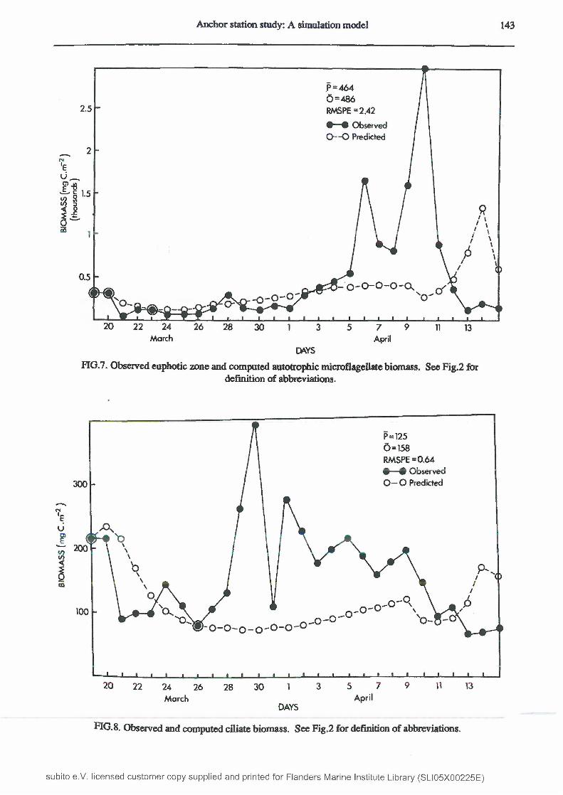
Model output of autotrophic microflagellate biomass closely followed the observed trend ifl euphotic-zone flagellates for the first 18 days, but then failed to simulate the bloom observed from 6 to 10 April and estimated a much smaller peak when this observed bloom had crashed. This discrepancy accounted for the lower simulated mean and for the RMSPE of 2.42 (Fig.7). In the model, the development of this bloom was prevented by ciliate grazing. The observed maximum was able to develop during a time of observed large ciliate biomass (Fig.8), and it is possible that the impact of ciliate grazing on autotrophic microfiagellates was overestimated in the model, at least over this period.

Computed ciliate biomass had the lowest RMSPE (0.64) o f all the biological groups examined (Fig.8). A peak from 29 March to 10 April was not fully reproduced by the model although the model did compute a slow increase in biomass over this period. Figure 9 shows the calculated biomasses of the bacteria and microzooplankton in the simulated system. The noticeable and surprising feature of this figure is the comparatively high biomass of the heterotrophic flagellates which considerably exceeded that of bacteria, the former’s sole food source. The c o m p u t e d

biomasses are a result of the potentially fast growth rate of bacteria (up to 6.0 times the initia* biomass per day) and low predation rates by ciliates on heterotrophic flagellates. The ciliates in the mode) are also able to utilise the autotrophic microfiagellates and to feed on them selves.

Computed mesozooplankton and macrozooplankton were marked by declines throughout the simulation period, which contrasted with the large fluctuations in the observed data (Figs 10 and



P = 4 2 9 0

5 =2883

RMSPE = 15.12

# —# Observed

O— O Predicted

' QCO XX

20 22 24 26 28 30 1 3 5 7 9 11 13

March April

DAYS

FIG.3. Observed and computed diatom biomass. See Fig.2 for definition of abbreviations.

EX

Diatoms

Dinoflagellates

Microfiagellates

n o 3 - N

40

20 22 324 28 30 5 726 9

March April

DAYS

HG.4. Depth below the surface of the computed peak biomass of diatoms, dinoflagellates and autotrophic flagellates and the depth of the zone of most rapid change in nitrate nitrogen (N 03-N)

during a model ran from 19 March to 9 April, just prior to the upwelling on 10 April.


142 KJL. C ochrane et ál.

“(O

20 26 30 1322 24 5 728 3 9 IIMarch April

DAYS

FTG.5. Vertical profile of computed chlorophyll concentrations (mg O il m‘3).

€>—• Observed

0 * - 0 PredictedP =404 0 = 378

RMSPE = 0.98

0.8

öl -ß E c

" í 0 6io o

CO

0.4

0.2

20March April

DAYS

FIG.6. Observed and computed dinoflagellate biomass. See Fig.2 for definition of abbreviations.



P = 464 0 = 480 RMSPE =2.42

• —• Observed O— O Predicted

2.5

«3

0.5¡ _ 0 ' 0 - o - o - a

o -

20 22 24 26 28 5 930 31 7 13March April

CAYS

FIG.7. Observed euphotic zone and computed autotrophic microflagellate biomass. See Fig.2 fordefinition of abbreviations.

P = 125 0 = 1 5 8 RMSPE =0.64# —# Observed 0 —0 Predicted300

r 200

100t>-

|- 0 - 0 ~ 0 - 0 '- ° - 0 " 0

20 97 U 1322 3 524 30 126 28March April

DAYS

FIG.8. Observed and computed ciliate biomass. See Fig.2 for definition of abbreviations.



O - - O Bacteria800 Heterotrophic flagellates

+ ......+ Ciliates

600

400

« jo-o.

O.

° —0 - 0 - ,200

20 24 1322 26 28 30 7 9 113 5March April

DAYS

FIG.9. Computed biomass of bacteria, heterotrophic flagellates and ciliates.

P = 2332 Ö - 2 311 RMSPE = 3.96 • — # Observed O— O Predicted

CO

0~Ö \-0-p-\~0-0~0-0~ 'Q Ä

\ I \ o - ° ' 0 - o - o

March AprilDAYS

FIG. 10 Observed and computed mesozooplankton biomass. See Fig.2 for definition of abbreviations.



11 ). The latter must incorporate variance from sampling error (VERHEYE, 1991 ) and patchiness, and the true trends in the two communities were probably considerably less erratic than indicated by the results. However, the model estimated daily grazing by fish to be aconstant function of prey availability whereas, in reality, it is more likely to be an erratic occurrence at any given locality, depending on the presence or absence of feeding shoals of fish. Thus predation could vary from zero to levels far in excess of model estimates from day to day. The true trend may, therefore, lie somewhere between those of the observed and simulated values. As with the cases discussed above, improvements to the goodness-of-fit would require both a three-dimensional model and better estimates of actual standing stock. The procedures for the meso- and macrozooplankton compartments are very simple and do not take into account the age-structure of the population or influx and advection of biomass. Such features could be built into a three-dimensional model and would be required if real improvements to the RMSPEs of 3.96 for mesozooplankton and 2.02 for macrozooplankton are to be made.

The model showed that the fish were able to feed to satiation on all days despite the decline in both meso- and macrozooplankton standing stocks. The computed standing stock of macrozooplankton did not respond to the increased primary production following the upwelling events on 10 and 15 April but the decline in mesozooplankton started to level off. These results, together with those of the sensitivity analysis, indicate that in the model macrozooplankton population losses to fish grazing exceeded the modelled production rate of the zoöplankton, even under the initial conditions of high food availability.

P = 1439 0 = 9 2 2 RMSPE = 2.02 # — # Observed O—O Predicted

<N'E0ifoCO

9 t320 7 113 522 2624 28 30M arch April

CAYS

FIG. 11. Observed and computed macrozooplankton biomass. See Fig.2 tor definitionof abbreviations.


146 K.L. C ochran e et aï.

6. DISCUSSION

6.1 Evaluation o f the model

In terms of the objectives listed in the introduction, the modelling exercise was largely successful. The results obtained in the field study were incorporated into a single model which was then used to evaluate interactions between the groups. The short duration of the study plus the fact that it was designed without consideration of the model requirements meant that several rates and variables had to be derived from the literature, estimated by calibration or, in some cases, assumed. While this unquestionably reduces the potential for using the model as apredictive tool, the modelling exercise helped to highlight uncertainties in our knowledge of the functioning of marine ecosystems driven by upwelling events.

6.1.1 Phytoplankton. The large biomass peaks which were not simulated by the model for the diatom and microflagellate groups indicate processes missing or not adequately represented in the model. The assumption of constant daily solar radiation for the duration of the study is a potential source of considerable error. In the case of the diatom procedure, other likely sources of error are the fixed light optimum for the group and their fixed sinking rate. In reality, results for different species of algae, including some diatom species, show that many species are able to increase their chlorophyll a content if light intensity is decreased during growth. This could permit the establishment of biomass maxima at depth (KIRK, 19B3, p.305). Improved knowledge of this process in the diatom species of the southern Benguela and the incorporation of a function of this nature, with the correct parameters, would enable the model to simulate the observed Coscinodiscus maximum.

Prediction of changes in the factors controlling light penetration through the water column, as newly upwelled water matures and the dominant phytoplankton species change could also improve the validity of the model. This would require improvement in the validity of parameters in the equation to calculate the extinction coefficient or improved definition of the relationship itself. Similarly, insight into the light optima of different phytoplankton groups and the relationship, if any, of these to nutrient availability and the age of the population, could help to overcome some of the discrepancies in the output values from the model.

The failure of the model to simulate the biomass peak of the diatoms at depth could also reflect the inadequacy of using a constant sinking rate for each of the three groups. ANDERSEN and NIVAL (1989) incorporated functions which related sinking rates of diatoms negatively to silica availability and positively to age. The incorporation of these functions, with appropriate parameters for the southern Benguela, could improve the goodness-of-fit and validity of the model during diatom blooms.

The model does suggest that the faster sinking rate of diatoms, in relation to the other groups, is a mechanism which enables diatoms to exploit the deeper, higher concentrations of nutrients more effectively than the other groups. This feature would, however, only be beneficial if coupled with the ability of the organisms to maintain high production at low light intensities, as was described for Coscinodiscus in this study (MITCHELL-INNES and WALKER, 1991). There is evidence that dinofiagellates are able to migrate vertically between areas of optimal nutrient availability and optimum light intensity (HEANEY and EPPLEY, 1981 ; TETT, 1987). However, the higher biomass of diatoms during much of the study indicates that this ability is insufficient for them to out-compete diatoms when euphoric nitrogen concentrations are high. The diatom population was able to maintain itself as long as net production in a stratum exceeded total losses,


Anchor Station study: A sim u la tio n m o d e l 147

including those through sinking. Thus the peak biomass in the water column was closely associated with the nutricline (Fig.4) until light limitation reduced production to the extent where the diatom community could neither fully utilise the available nitrogen nor maintain a high density in the vicinity of the nutricline. At this point the simulation implied that the community of diatoms continued to sink below the nutricline and would have ultimately disappeared had it not been for the second upwelling event which, in the model, redistributed the diatom biomass in the water column. In the real system, upwelling events reseed the area with entirely new diatom populations (PITCHER, WALKER, MITCHELL-INNES and MOLONEY, 1991).

Mesozooplankton were estimated to have the major impact on diatom losses through grazing, while ciliates exerted a significant influence on autotrophic microflagellate dynamics. Better knowledge of the actual relationships between the ciliates and microflagellates would have helped to eliminate the large residuals obtained during the microflagellate bloom. It could be postulated that the microflagellates have a higher maximum growth rate than the lOmgC.mgChl^h'1 used in the model but that, through loss or limitation, this was not realised at the study site except during the major bloom. Further study into the dynamics and loss processes affecting the <10pm phytoplankton fraction is also required.

Some of the short-term fluctuations observed in all the measured state variables, such as the sudden increase in dinoflagellate biomass from 30 March to 5 April, could reflect patchiness in the spatial distributions of these organisms in the study area. This is a short-coming in one fundamental assumption of the model, that of a homogeneous water-body, and points to the need both for wider-scale sampling to obtain better estimates of actual biomass, and for three- dimensional models. However, it is unlikely that a reliable and accurate three-dimensional model could be developed with sufficient resolution to simulate patchiness on this scale.

6.12. Microheterotrophs. The simulation of the microheterotrophic groups cannot be completely assessed in the absence of observations on bacterial and flagellate standing stocks, but die goodness-of-fit of the ciliate component does support their general validity. The prediction dm the flagellate biomass is consistently higher than that of bacteria is counter-intuitive, but the parameters used in these groups all fall within realistic ranges, and the results demonstrate that such a scenario is feasible even if it did not acctually occur during this study. A microcosm study which used newly upwelled water from the southern Benguela, examined interactions between bacterivorous flagellates and bacteria (LUCAS, PROBYN and PAINTING, 1987). In this study a bacterial community which developed initially and supported a flagellate community, grew rapidly and ultimately exceeded the bacterial biomass for a period of approximately 5 days before u Was rePlaced by larger bacteria. No mention was made of predators on the flagellates. Similar results, expressed as numbers instead of biomass, were also found in cultures using water from

arhus Bay, Denmark (ANDERSEN and FENCHEL, 1985). The relatively stable bacterial biomass, uctuating between 66.6 asnd 329.0 mg C n r2, is consistent with observations that bacterial

numbers remain fairly constant with time (ANDERSEN and FENCHEL, 1985).6-13. Mesozooplankton and macrozooplankton. The mesozooplankton and macrozooplank-

0n Procedures were extremely simple and incorporated neither age nor size structure nor Ontogenetic migration which is a feature of some Zooplankton groups in the southern Benguela 'including the mesozooplanktonic Calanoides carinatus (VERHEYE, 1989) and the euphausiid ^ y usia lucens in the Benguela system (pillar and STUART, 1988; VERHEYE and ch CHrNGs> 1988; PILLAR, ARMSTRONG and HUTCHINGS, 1989; VERHEYE, 1991) and may be ^uracteristic of other representatives of the two categories of Zooplankton. The observed data o*re marked by substantial fluctuations, probably reflecting heterogeneous distribution of

ganisms in the water. It is, therefore, not surprising that the model captured only the basic trend


148 K J L C o c h ra n e et al.

of the observed communities, which was a net decrease until or just prior to the second upwelling. The mesozooplankton were most sensitive to food-related parameters and, with relatively minor changes in food, particularly diatom availability, it was possible to cause the simulated population to increase. The macrozooplankton were insensitive to 10% changes in any food- or growth- related parameters and were driven by predation. These opposing features reflected the differences in maximum growth rate of the two groups. The mesozooplankton had a minimum doubling time of 3.3 days while the macrozooplankton minimum was 16.7 days. Therefore, with favourable food availability, mesozooplankton would be able to recover from heavy predation more rapidly than the larger Zooplankton.

The assumption that respiration by the heterotrophs is directly related to biomass could be improved upon. STEELE (1974, p.66) suggested that respiration rate would be proportional to food intake and the use in the model of a relationship of this nature should be investigated.

The model computed that macrozooplankton biomass was declining throughout the simulation and that this trend was not sensitive to the perturbations in food availability induced in the sensitivity analysis. No such robust decline was apparent in the observed population, which stabilised at the lower levels and started to increase after the second upwelling event The discrepancy between model output and observations could have been the result of: (1) an overestimate of actual fish biomass or ingestion rate or both; (2) an underestimate of macrozooplankton biomass and production, or (3) the assumption of continuous “mean” rates of feeding rather than the sporadic invasions of fish which would be more typical o f the real environment

The observed fluctuations of both Zooplankton size groups could have been a reflection of patchiness in distribution but could also be interpreted as showing an initial collapse caused by heavy predation between 21 and 23 March, followed by low levels thereafter (Figs 10 and 11). This could be explained by dense fish populations and predation at the study site up to 23 April, followed by substantially lower predation thereafter, such that losses were b e t t e r compensated for by production and immigration. Clearly it would be impractical to simulate such a sequence in a one-dimnensional, deterministic model, but the model could be used for stochastic investigations of the impact of fish-feeding and could be extended to a three-dimensional model incorporating migration, again with fish-feeding best simulated stochastically. In a future study, a simultaneous monitoring of fish abundance and diet would be of considerable advantage.

6.1.4. Fish. Food did not appear to be limiting to fish in this area. In reality, the distribution of fish would be highly clumped, and the observed data showed more than order-of-magnitude variations in both meso- and macrozooplankton. Thus the real feeding environment would differ markedly from the assumption of mean fish density feeding on mean plankton density used in d* model. Nevertheless, the results show that, on average, fish would be able to acquire their daily needs, and there was no evidence of food limitation for fish in St Helena Bay at this time. However, St Helena Bay is an important area for anchovy and sardine recruits to the fishery and HAMPTON (1987) found densities of anchovy greater than lOOtknr2 in this area in May 1985 and June 1986, compared with the 22.84t km"2 measured in February 1987. It is, therefore, possible that food limitation could occur during the austral winter when recruit abundance is particularly high intte St Helena Bay vicinity. The fish may be even more vulnerable to death by starvation at the eariiitf stages of their life cycle (LASKER, 1985), and the model could be used to investigate fooà limitation during this period in specific nursery areas.



6.2 The future development and potential use o f the model

The number of uncertainties and the imprecision of a large number o f the parameters used in the model, and in other similar models, at present prevent their use as tools to predict biomass or production of the functional groups represented in them. Such models should be viewed as hypotheses to explain the gross features of system dynamics which can be evaluated as additional results become available, refined as knowledge improves or scrapped if found to be false. The formal and explicit nature of a systems model provides an unambiguous structure on which to summarise the best current ideas on systems functioning for future re-evaluation and testing (WALTERS, 1986, p.45). Used in this way, models can also provide invaluable guides in determining future sampling and experimental programmes.

In simulation modelling, as in empirical modelling, the discrepancy between predicted and observed, the residuals, can frequently be more informative than the goodness-of-fit itself. These residuals highlight some of the more important uncertainties in quantification of community dynamics in the St Helena Bay system, as has been demonstrated above.

The construction of the model, the sensitivity analysis undertaken on it and the attempts to calibrate it have all revealed uncertainties in existing knowledge of the functioning of the ecosystem and in the rates of various processes. Two additional steps will assist further in the development of the model. These are: (1) a comprehensive sensitivity analysis, and (2) attempts to validate the model by applying it to the existing, applicable data sets or to a new data set collected for this purpose.

Insights gained from the above, in conjunction with those obtained from this initial exercise, could lead to improvements in the model, in the form of structural or parameter changes. Once confidence has been gained in an improved model, it should be possible to use it to assist in the design of plankton sampling and monitoring exercises and in the preliminary testing of related hypotheses, prior to their validation in the field or laboratory. As suggested above, the model could also be used to investigate relationships between pelagic fish and their food. It may prove desirable to use the model as the biological basis of a three-dimensional model of, for example, the spawning areas of the piichard and anchovy, which could then be used to investigate feeding during the spawning and larval stages of anchovy and pilchard in more detail.

7. CONCLUSIONS

The construction of the model has assisted in identifying the following key areas that require additional research:

1. Inter-relationships between light and the phytoplankton groups.2. Autotrophic microflagellate dynamics in relation to their abiotic and biotic

environment.3. Standing stocks of bacteria and heterotrophic flagellates in Benguela plank

tonic systems.4. Patchiness in the distribution of all biotic groups and its impact on predator-

prey encounters.5. Horizontal distribution o f meso- and macrozooplankton and the patterns of

recruitment to the older stages.6. In situ feeding behaviour and shoal densities of pelagic fish, particularly the

larval and juvenile stages.



The development and examination of the model has given some additional insight into the functioning of the St Helena Bay planktonic ecosystem. The importance of the light environment and the adaptations of different phytoplankton groups to this environment were demonstrated, as was the significance of nutrient stratification in relation to light The role of competition for nitrogen between the phytoplankton groups was also seen to be important, and the passive sinking of diatoms, coupled with adaptation to low light intensities, appeared to assist rapid exploitation of nitrogen in a sinking nutricline. Losses to grazers played a role in the dynamics of all three groups.

Ciliates had an impact on microflagellate abundance and were themselves kept at relatively low levels by predation, despite periodic large standing stocks of both autotrophic and heterotrophic flagellates. The model indicated that mesozooplankton were able to respond to changes in food availability, particularly diatom standing stocks, while feeding by fish steadily drove the macrozooplankton population towards extinction in the model community, suggesting that horizontal advection of new Zooplankton biomass may be important in areas of high fish density.

The model described above is the first attempt to incorporate all the major groups, from microbes to fish, in a single simulation model of the Benguela ecosystem. Overall, it provided a reasonable first estimate of the major trends in biomass of a highly dynamic and interactive community, where indirect effects had considerable influence on the abundance of the components. Finally, the model provided a valuable tool for synthesising and evaluating these interactions in a framework that can be replicated and rigorously tested and can be developed in parallel with new results.

8. ACKNOWLEDGEMENTS

The authors express their thanks to Mr Geoff Bailey, Sea Fisheries Research Institute, for his role in the fixed anchor station study as a whole and for advice and comments on the structure of the model.Mrs Dot Armstrong provided useful feedback during the construction of the model and Prof. John Field, University of Cape Town, and Dr Larry Hutchings, Sea Fisheries Research Institute, madehelpful suggestions on the manuscript.

9. REFERENCES

ANDERSEN, P. and T. FENCHEL (1985) Bacterivoiy by microheterotrophic flagellates in seawater samples- Limnology and Oceanography, 30 ,198-202.

ANDERSEN, V., and P. NIVAL (1989) Modelling of phytoplankton population dynamics in an enclosed watet column. Journal of the Marine Biological Association of the United Kingdom, 69,625-646.

ANDERSEN, V., P. NTVAL and RP. HARRIS (1987) Modelling of a planktonic ecosystem in an enclosed wsW column. Journal of the Marine Biological Association of the United Kingdom, 67,407-430.

ANGEL, M.V. (1984) Detntal organic fluxes through pelagic ecosystems. In: Flows of energy and materials in marine ecosystems, M. FASHAM, editor, Plenum, 475-516.

BAILEY, G.W. and P. CHAP MAN (1991) Short-tram variability during an anchor station study in the south**® Benguela upwelling system: Chemical and physical oceanography. Progress in Oceanography, 28,9-37-

BROWN, P.C. and J.G. FIELD (1986) Factors limiting phytoplankton production in a nearshore upwelling are*- Journal of Plankton Research, 8,55-68.

BROWN, P.C. and L.C. HUTCHINGS (1985) Phytoplankton distribution and dynamics in the southern Bengueti current. In: International symposium on the most important upwelling areas off western Africa (UnPe Blanco and Benguela), Instituto de Investigaciones Pesqueras, Barcelona, 1,319-344.

CHAPMAN, P. and G.W. BAILEY (1991) Short-term variability during an anchor station study in the south**® Benguela upwelling system: Introduction. Progress in Oceanography, 28,1-7.

CHAPMAN, P. and L.V. SHANNON (1985) The Benguela Ecosystem. Part ü. Chemistry and related processes. Oceanography and Marine Biology. An Annual Review, 23,183-251.



COCHRANE, K.L., P. J. ASHTON, A.C. JARVIS, A.J. TWINCH and T. ZOHARY (1987) An ecosystem model of phosphorus cycling in a warm monomictic, hypertrophic impoundment Ecological Modelling, 37, 207- 233.

CRAWFORD, R. J.M., L.V. SHANNON and D.E. POLLOCK (1987) The Benguela Ecosystem. Part IV. The major fish and invertebrate resources. Oceanography and Marine Biology. An Annual Review, 25 ,353-505.

CUSHING, D.H. (1983) The outlook for fisheries research in the next ten years. In: Global Fisheries. Perspectives for the 1980s. B.J. ROTHSCHILD, edite», Springer-Verlag, 263-277.

FENCHEL, T. and B. J. FENLA Y (1983) Respiration rates in heterotrophic, free-living Protozoa. Microbial Ecology, 9 ,99-122.

FROST, B.W. (1987) Grazing control of phytoplankton stockin the open subarctic Pacific Ocean: a model assessing the role of mesozooplankton, particularly the large calanoid copepods Neocalanus spp. Marine Ecology - Progress Series, 39,49-68.

HAMPTON, L (1987) Acoustic study on the abundance and distribution of anchovy spawners and recruits in South African waters. In: The Benguela and Comparable Ecosystems, A.I.L. PAYNE, J. A. GULLAND and K.H. BRINK, editors, South African Journal o f Marine Science, 5 ,901-917.

HARRIS, G.P. (1978) Photosynthesis, productivity and growth; the physiological ecology of phytoplankton.Ergebnisse der Limnologie, 10,17.

HEANEY, S.I. andR.W. EPPLEY(1981)Light, temperature andnitrogen as interactingfactors affecting diel vertical migrations of dinoflagellates in culture. Journal of Plankton Research, 3,331-344.

HEARNE, J.W. (1985) Sensitivity analysis of parameter combinations. AppliedMathentaticsandModelling, 9,106- 108,

HOFMANN, E.E. and J.W. AMBLER (1988) Plankton dynamics on the outer southeastern U.S. continental shelf.Part H: A time-dependent biological model. Journal of Marine Research, 46,883-917.»

JAMES, A.G. (1987) Feeding ecology, diet and field-based studies on feeding selectivity of the Cape anchovy Engraulis capensis Gilchrist. South African Journal of Marine Science, 7 ,673-692.

JAMES, A.G. and K.P. FINDLAY (1989) Effect of particle size and concentration on feeding behaviour, selectivity and rates of food ingestion by the Cape anchovy Engraulis capensis. Marine Ecology - Progress Series, 50, 275-294.

KIRK, J.T.O. (1983) Light and photosynthesis in aquatic ecosystems. Cambridge University Press, 401pp. LAMBERTH, R. and G. NELSON (1987) Field and analytical drogue studies applicable to the St Helena Bay area

off South Africa’s west coast. In: The Benguela and Comparable Ecosystems, ALL. PAYNE, J A. GULLAND and K.H. BRINK, editors, South African Journal of Marine Science, 5 ,163-169.

LASKER, R. (1985) What limits clupeoid production? Canadian Journal of Fisheries and Aquatic Sciences, 42 ,31- 38.

UVINGSTON P.A and B J , GOJNEY (1984) Bibliography on daily food ration of fishes, NOAA Technical Memorandum NMFS FINWC-63, National Oceanic and Atmospheric Administration, National Marine Fisheries Service, 60pp.

LUCAS, M.I., T.A. PROBYN and S J. PAINTING (1987) An experimental study of microflagellate bactenvory: further evidence for die importance and complexity of microplanktonic interactions, hi: The Benguela and Comparable Ecosystems, ALL. PAYNE, JA . GULLAND and K.H. BRINK, editors, South AfricanJournal of Marine Science, S, 791-808.

makuaLEF, R. (1978) Life-forms of phytoplankton as survival alternatives in an unstable environment. OceanologicaActa, 1 ,493-509.

MITCHELL-INN ES, B A and D.R. WALKER (1991) Short-term variability during an anchor station study in the southern Benguela upwelling system: Phytoplankton production and biomass in relation to species’

Un chan8es- Progress in Oceanography, 28,65-89.LONE Y, CL. (1988) a size-based model of carbon and mtrogenflows in plankton communities. Ph.D. thesis,

Mnr University of Cape Town, 256pp.MOLONEY, C.L. and J.G. FIELD (1990) General allometric equations ft» rates of nutrient uptake, ingestion, and u respiration in plankton organisms. Limnology and Oceanography, 3 4 ,1290-1299.MOLONEY, C.L., M.O. BERGH, J.G. FIELD and R.C. NEWELL (1986) The effect of sedimentation and microbial

nitrogen regeneration in a plankton community: a simulation investigation. Journal o f Plankton Research, 8,427-445.

NEWELL, R.C. and C.M. TURLEY (1987) Carbon and nitrogen flow through pelagic microheterotrophic communities. In: The Benguela and Comparable Ecosystems, A.I.L. PAYNE, J.A. GULLAND and K.H.

p. BRINK, editors, South African Journal of Marine Science, 5,717-734.* MINTING, S.J., M.I. LUCAS and D.G. MUIR (1989) Fluctuations in heterotrophic bacterial community structure,


152 K i . C ochrane et al.

activity and production in response to development and decay of phytoplankton in a microcosm. Marine Ecology - Progress Series, 5 3 ,129-141.

PARSONS, T.R. and M. TAKAHASHI (1973) Biological Oceanographic Processes, Pergamon Press, 186pp.PETERSON, W.T. andD.C. BELLANTONI (1987) Relationships between water column stratification, phytoplank

ton cell size and copepod fecundity in Long Island Sound and off central Chile. In: The Benguela and Comparable Ecosystems, ALL. PAYNE, J.A. GULLAND and K.H. BRINK, editors, South African Journal of Marine Science, 5 ,411-421.

PILLAR, S.C. (1986) Temporal and spatial variations in copepod and euphausiid biomass off the southern and southwestern coasts of South Africa in 1977/78. South African Journal of Marine Science, 4,219-229.

PILLAR, S.C. and V. STUART (1988) Population structure, reproductive biology and maintenance of Euphausia lucens in the southern Benguela Current Journal of Plankton Research, 10,1083-1098.

PILLAR, S.C., D.A. ARMSTRONG and L. HUTCHINGS (1989) Vertical migration, dispersal and transport of Euphausia lucens in the southern Benguela Current Marine Ecology - Progress Series, 53,179-190.

PITCHER, G.C., D.R WALKER and B.A. MITCHELL-INNES (1989) Phytoplankton sinking rate dynamics in (he southern Benguela upwelling system. Marine Ecology - Progress Series, 55,261-269.

PITCHER, G.C., D.R. WALKER, BA. MITCHELL-INNES and C.L. MOLONEY (1991) Short-term variability during an anchor statical study in the southern Benguela upwelling system: Phytoplankton dynamics. Progress in Oceanography, 28,39-64.

PLATT, T., K.L. DENMAN and A.D. JASSBY (1977) Modeling the productivity of phytoplankton, hi: The Sea Volume 6: Marine Modelling, E.D. GOLDBERG, I.N. McCAVE, JJ. O’BRIEN and J.R STEELE, editors, John Wiley & Sons, pp. 807-856.

SHANNON, L.V. and J.G. FIELD (1985) Are fish stocks food-limited in the southern Benguela pelagic ecosystem? Marine Ecology - Progress Series, 22,7-19.

SHANNON, L.V. and S.C. PILLAR (1986) The Benguela Ecosystem. Part HL Plankton. Oceanography and Marine Biology. An Annual Review, 24,65-170.

STEELE, J.H. (1974) The structure of marine ecosystems, Blackwell, 128pp.STUART, V. (1986) Feeding and metabolism of Euphausia lucens (Euphausiacea) in the southern B e n g u e la Current

Marine Ecology - Progress Series, 30,117-125.STUART, V. and S.C. PILLAR (1990) Diel grazing patterns of all ontogenetic stages of Euphausia lucens and is

situ predation rates on copepods in the southern Benguela upwelling region. Marine Ecology - Progress Series, 64,227.241.

SWART, J. (1987) Sensitivity of a hyrax-lynx mathematical model to parameter uncertainty. South African Journal of Science, 83,545-547.

TETT, P. (1987) The ecophysiology of exceptional blooms. Rapports et Procès-Verbaux des Réunions, 187,47-60.VERHEYE, RM. (1989) Distribution, dynamics and production of the copepod Calanoides carinatus (Krpyer,

1849) in the southern Benguela upwelling region. PhD. thesis, University of Cape Town, 238pp.VERHEYE, H.M. (1991) Short-term variability during an anchor statical study in the southern Bragueta upwelling

system: Abundance, distribution and estimated production of mesozooplankton with special reference to Calanoides carinatus (Kr0yer, 1849). Progress in Oceanography, 28,91-119.

VERHEYE, H.M. and L. HUTCHINGS (1988) Horizontal and vertical distribution of Zooplankton biomass in ft® southern Benguela, May 1983. South African Journal of Marine Science, 6,255-265.

VERIFY, P.G, and C. LANGDON (1984) Relationships between lorica volume, carbon, nitrogen, and ATPcontsá of tintinnids in Narragansett Bay. Journal of Plankton Research, 6 ,859-868.

WALDRON, H.N. and TA. PROBYN (1991) Short-term variability during an anchor station study in tibe southern Benguela upwelling system: Nitrogen supply to the euphoric zone during a quiescent phase in the upwelling cycle. Progress in Oceanography, 28,153-166.

WALSH, J .J. (1975) A spatial simulation model of the Pera upwelling ecosystem. Deep-Sea Research, 22,201-236.WALTERS, C.J. (1986) Adaptive management of renewable resources, Macmillan, 374pp.WALTERS, C.J., E. KRAUSE, W.E. NEILL and T.G. NORTHCOTE (1987) Equilibrium models for season*!

dynamics o f plankton biomass in four oligotrophic lakes. Canadian Journal of Fisheries and Aquatic Sciences, 44,1002-1017.


Short-term variability during an anchor station study in ...

Documents

Transcript of Short-term variability during an anchor station study in ...