Short-term Forecasting of Reimbursement for Dalarna · PDF fileShort-term Forecasting of...
22
Short-term Forecasting of Reimbursement for Dalarna University One year master thesis in statistics 2008 Authors: Jianfeng Wang &Xin Wang Supervisor: Kenneth Carling
Transcript of Short-term Forecasting of Reimbursement for Dalarna · PDF fileShort-term Forecasting of...
Short-term Forecasting of Reimbursement for Dalarna
University
One year master thesis in statistics 2008
Authors: Jianfeng Wang &Xin Wang
Supervisor: Kenneth Carling
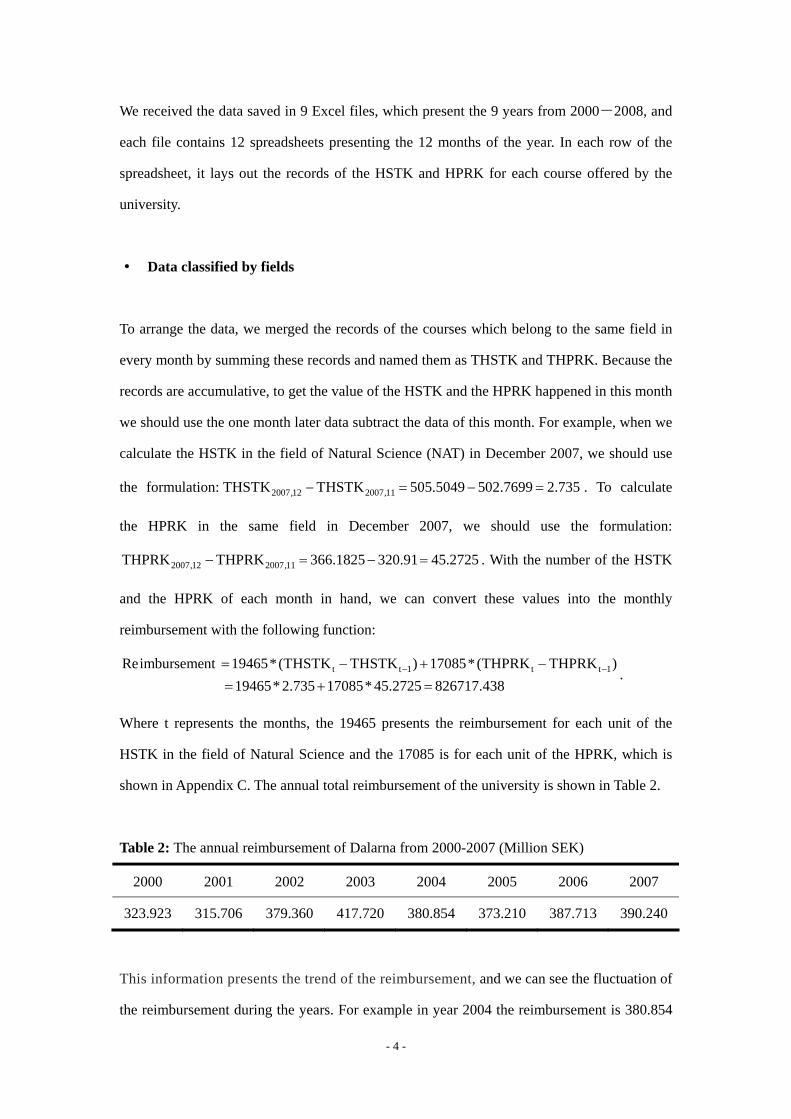
Abstract
Swedish universities are reimbursed by the government according to a scheme related to the
registration of students (HSTK) and the students’ performance (HPRK). On a disaggregated
level, such as a department or a field, the reimbursement is uncertain as the number and
performance of students are fluctuant. So the administration faces the challenge to balance the
reimbursement and the expense. In this thesis, we try to distinguish a better forecasting model
for the educational fields or the departments of Dalarna University. We analyze the time series
by two methods, namely Census II method and the ARIMA method. We apply the two methods to
two approaches, direct and indirect approaches. The first one is to use the time series of
reimbursement directly; the second one is to forecast the number of students and their
performance separately, and then convert these two forecasted values into reimbursement. To
compare the results, we choose the indication of MAPE. We use monthly data from Jan. 2000 to
Feb. 2008. Finally, we find that, on the department level, the ARMA model of the indirect
approach is the best one for forecasting the reimbursement.
Keywords: Census II Method, ARMA Method, MAPE

Contents
1. Introduction............................................................................................................................ - 1 -
2. Data Description..................................................................................................................... - 3 -
3. Method .................................................................................................................................... - 5 -
4. Results for the Field of Natural Science ............................................................................... - 6 -
5. Comparison between the Census II Method and the ARMA Method............................. - 11 -
6. Conclusion ............................................................................................................................ - 15 -
Reference................................................................................................................................... - 16 -
Appendix................................................................................................................................... - 17 -

- 1 -
1. Introduction
In Sweden, the reimbursement for the higher education sector is always increasing until
recently. In 2004, the reimbursement became to decline partly because the educational
institutions enrolled less students than before1 as the reimbursement is highly related to the
number and the performance of the college students. To some extent, the reimbursement for a
university will fluctuate around a trend. Our thesis is to establish an accurate model to
forecast the reimbursement for the fields or the departments in the university. The model may
help them to balance their expense and reimbursement better. In this thesis, we take the
Dalarna University as an example.
Figure 1 shows the number of students registered in 1990-2005. In 2005, the total volume of
higher education comprised 295,150 full-time students. This is a reduction of 2.5 percent
compared with the previous year and this is the first time for twenty years that the number of
full-time students declined2.
Dalarna University was established in 1977. Today there are about 10 000 students studying
1 http://hsv.se/statistics/theannualreport.4.539a949110f3d5914ec800064188.html 2 http://www.hsv.se/download/18.539a949110f3d5914ec800081527/0638R.pdf
Figure 1: The number of full time equivalent (FTE) students in Sweden Source: 2005 Annual Report of Swedish National Agency for Higher Education
Num
ber
Year

- 2 -
in this university. Distance education is also offered in various forms. There are more than
200 courses within the areas of welfare, business, infrastructure media, culture and tourism
and so on3. All of the courses are classified into 11 fields: the Humanity, Sport, Law,
Education, Media, Medicine, Natural Science, Social Science, Technique, Health and Care,
and the Others, the amount of the reimbursement depends on these fields. The courses can
also be classified into 5 departments: Culture, Social, Health, Humanity, and Industry. The
fields and the departments at Dalarna University are shown in Table 1.
Table 1: The share of the fields and departments in terms of the average reimbursement from 2000 to 2008 (%)
Department
Field
Culture Social Health Humanity Industry Marginal size
Other 8.59 0.01 6.56 3.80 2.63 2.21
Humanity 5.39 0.14 0.76 55.60 0.27 7.33
Sport - 1.21 1.71 - - 0.48
Law - 13.07 16.90 - - 1.76
Education 0.83 1.96 20.86 38.96 2.69 12.00
Media - 10.47 22.82 - - 16.80
Medicine 31.31 - - - - 4.45
Natural Science 2.54 17.01 3.16 0.95 56.04 11.90
Social Science 11.10 42.84 19.31 1.06 - 10.90
Technique 45.89 22.05 - - 40.01 21.70
Care 0.72 1.18 16.83 - - 10.40
Marginal size 17.10 14.60 39.70 11.80 16.80 100.00
This table shows the size each field takes up in the departments and the marginal size of the
departments and the fields in Dalarna University. For example the field Humanity takes up
5.39 % in the Culture department, and about 7.33 % in this school and the Culture department
takes up 17.1 %. From this table we can see the Sport field is the smallest one, whereas the
3 http://du.se/Templates/StartPage____1622.aspx?epslanguage=SV

- 3 -
Technique field is the largest one.
The key of this thesis is that we classified the data not only by the fields, but also by the
departments. To forecast the reimbursement, we choose two approaches: the direct approach
and the indirect approach. The first one is to use the time series of the reimbursement directly;
the second one is to forecast the number of students and their performance separately and then
convert these forecasted values into the reimbursement. We use two methods, namely the
Census II method and the ARIMA method, to model these two approaches on the field level
and the department level.
2. Data Description
We use the monthly data from Jan. 2000 to Feb. 2008. The Swedish universities are
reimbursed by the government according to a simple scheme related to the registration of the
students and the student’s performance. The allocation rule of the reimbursement is: 60% of
the reimbursement is based on the registration and 40% is based on the performance4. In this
thesis, we use HSTK as the short form for the registration of the students and HPRK for the
performance. We get the data of HSTK and HPRK from all the courses. All the courses are
classified into 11 fields and how the reimbursement depends on fields is shown in the table A
and B of the Appendix C. The HSTK is calculated by the number of registered students
multiplying with the credits of the course and dividing by 60 credits which is the total number
of credit points for one year full-time study. The calculating method of the HPRK is similar to
the HSTK. The only difference is the number of registered students is changed into the
number of students who have passed the examination. The two formulations are shown
below:
HSTK = number of registered students ×credits of the course /60
HPRK = number of students who have passed the exam ×credits of the course /60
4 The Annual Report of Swedish National Agency for Higher Education http://hsv.se/statistics/theannualreport.4.539a949110f3d5914ec800064188.html
- 4 -
We received the data saved in 9 Excel files, which present the 9 years from 2000-2008, and
each file contains 12 spreadsheets presenting the 12 months of the year. In each row of the
spreadsheet, it lays out the records of the HSTK and HPRK for each course offered by the
university.
Data classified by fields
To arrange the data, we merged the records of the courses which belong to the same field in
every month by summing these records and named them as THSTK and THPRK. Because the
records are accumulative, to get the value of the HSTK and the HPRK happened in this month
we should use the one month later data subtract the data of this month. For example, when we
calculate the HSTK in the field of Natural Science (NAT) in December 2007, we should use
the formulation: 2007,12 2007,11THSTK THSTK 505.5049 502.7699 2.735− = − = . To calculate
the HPRK in the same field in December 2007, we should use the formulation:
2007,12 2007,11THPRK THPRK 366.1825 320.91 45.2725− = − = . With the number of the HSTK
and the HPRK of each month in hand, we can convert these values into the monthly
reimbursement with the following function:
t t 1 t t 1Reimbursement 19465*(THSTK THSTK ) 17085*(THPRK THPRK )19465* 2.735 17085* 45.2725 826717.438
− −= − + −
= + =.
Where t represents the months, the 19465 presents the reimbursement for each unit of the
HSTK in the field of Natural Science and the 17085 is for each unit of the HPRK, which is
shown in Appendix C. The annual total reimbursement of the university is shown in Table 2.
Table 2: The annual reimbursement of Dalarna from 2000-2007 (Million SEK)
2000 2001 2002 2003 2004 2005 2006 2007
323.923 315.706 379.360 417.720 380.854 373.210 387.713 390.240
This information presents the trend of the reimbursement, and we can see the fluctuation of
the reimbursement during the years. For example in year 2004 the reimbursement is 380.854
- 5 -
million SEK.
Data classified by departments
In the original data, we do not have the level of the reimbursement for departments. To
calculate the reimbursement of each department, firstly we merged the records of the courses
which belong to the same department in every month, and then in each department we merged
the records of the courses which belong to the same field. After these procedures, with the
same calculating method for the field just as we stated above, we can get the reimbursement
of the department. Then we got the true value happened in every month. Then we had
monthly time series data for 9 years for each of the departments.
3. Method
To forecast the reimbursement for one field or one department, we consider two approaches,
namely indirect and direct approaches. The reimbursement is determined in a simple way. Let
y be the reimbursement of one field or one department, z denotes the number of the HSTK,
and w denotes the number of the HPRK. Then we have the formulation:
t 1 t 2 ty c *z c * w= + (1).
Where the constants 1c and 2c are the reimbursement depending on the field and shown in
Appendix C. The direct approach is to model ty directly, where ty is a function of past
value of y say t t 1y , y ... ...− , and time t, t 1... ...− . For the indirect method, first we forecast the
tz and tw separately, which means we build one model for tz , a function of
t t 1z ,z ......, t, t 1......− − and one for the tw , a function of t t 1w ,w ......, t, t 1......− − then
convert the two forecasted values into reimbursement calculated by equation (2).
t 1 t 2 tˆ ˆ ˆy c *z c * w= + (2).
Where the " "Λ means the predicted value. To get the model we choose the Census II

- 6 -
method and the ARIMA method.
Firstly, we introduce the knowledge of the Census II method. Any time series X is composed
of trend (T), season (S), cycle (C), and random influences (E). This method is to derive the
trend, season, and other components from X. There are two common models:
Multiplicative: X = (T × C)×S ×E
Additive: X = (T + C)+ S + E
In this thesis we choose the additive method, because the multiplicative model is commonly
used for the growth curve rather than stationary curve. Another reason why we choose the
additive model is that the original data contains the 0 value, which can not be transacted by
the multiplicative model. The main step of the Census II is computing T+C by moving
average and then get S+E=X-(T+C). Then get S by moving average and calculate X-S =
T+C+E, the seasonal adjusted value. In this process, we use the moving average many times.
Finally we can calculate the value of tX : tˆ ˆˆ ˆX T C S= + + . All these steps are performed with
statistic software Eviews 3.
We also tried the ARIMA model (Autoregressive Integrated Moving Average model). The
main procedure of this model is explained as follow: when we get the observed series, the
first thing is to decide if the series is stationary. We use the test of unit root to test if the series
is stationary. We found that the data is stationary and hence we need not to difference the
series. Then we can construct an ARMA model, and check whether the residuals of the
ARMA model are white noise. If not, we repeat the procedure above, if so, the procedure is
over.
4. Results for the Field of Natural Science
There are 11 fields and 5 departments in Darlarna University and it would be too many to
show all the results. Instead we will describe the modeling process of the field of Natural
Science as an example. The proceeding is similar for the other fields and the departments.
Summary results are given in sections 5 and 6.

- 7 -
After removing the seasonal factor, we get the seasonal adjusted series of the HSTK in the
field Natural Science.
Figure 2: Seasonal adjusted series of the registration in the field Natural Science
Let *tz be the seasonal adjusted series. We try several functions to model *
tz , such as the
error function, logistic transform, linear function of t and t ^n and log function and so on. In
Table 3 we show the AIC for some competing models.
Table 3: The Values of AIC for competing models
F u n c t i o n A I C
E r r o r F u n c t i o n 9 . 5 5
L o g i s t i c T r a n s f o r m 9 . 5 8
L i n e a r F u n c t i o n o f t a n d t ^ n 9 . 8 9
L o g F u n c t i o n 9 . 8 5
According to AIC, we would like to choose the Error Function:
This is a function of *tz and t; b is a parameter to be estimated. The residuals of the model
pass the white noise test. So the model is reasonable. Then we show the graph of seasonal
2t* zt 0
2z b * e dz M A (1)π
−= +∫
Year
HST
K

- 8 -
factor in Figure 3:
Figure 3: Seasonal factor series of the registration in the field Natural Science
Let tz′be the seasonal factor series. According to the formulation:
ˆ tz = *ˆ tz + ˆ ′tz (3)
So we can calculate the value of the ˆ tz . Figure 4 shows linear graph of the forecasted data
and the original data.
Figure 4: Comparison between original value and forecasted value of the registration in the
field Natural Science
The correlation of ˆ tz and tz is 0.92. We also check the index of mean absolute
HST
K
Year
HST
K
Year
- 9 -
percentage error (known as
n
t t tt 1
z z / zMAPE *100%
n=
−=∑
). When n=6, it equals to 22.66 %.
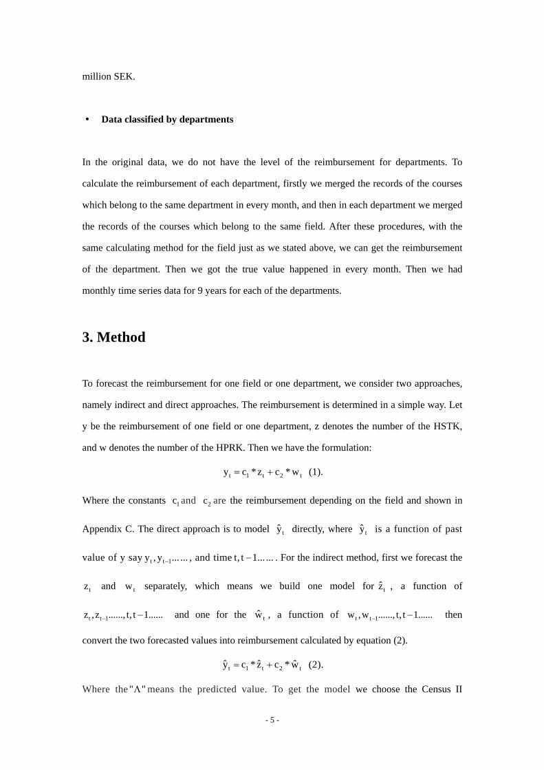
The analysis of the HPRK is similar as the HSTK. Let *tw be the seasonal adjusted series,
′tw be the seasonal factor series. The graph of seasonal adjusted is shown below:
Figure 5: Seasonal adjusted series of performance in the field Natural Science
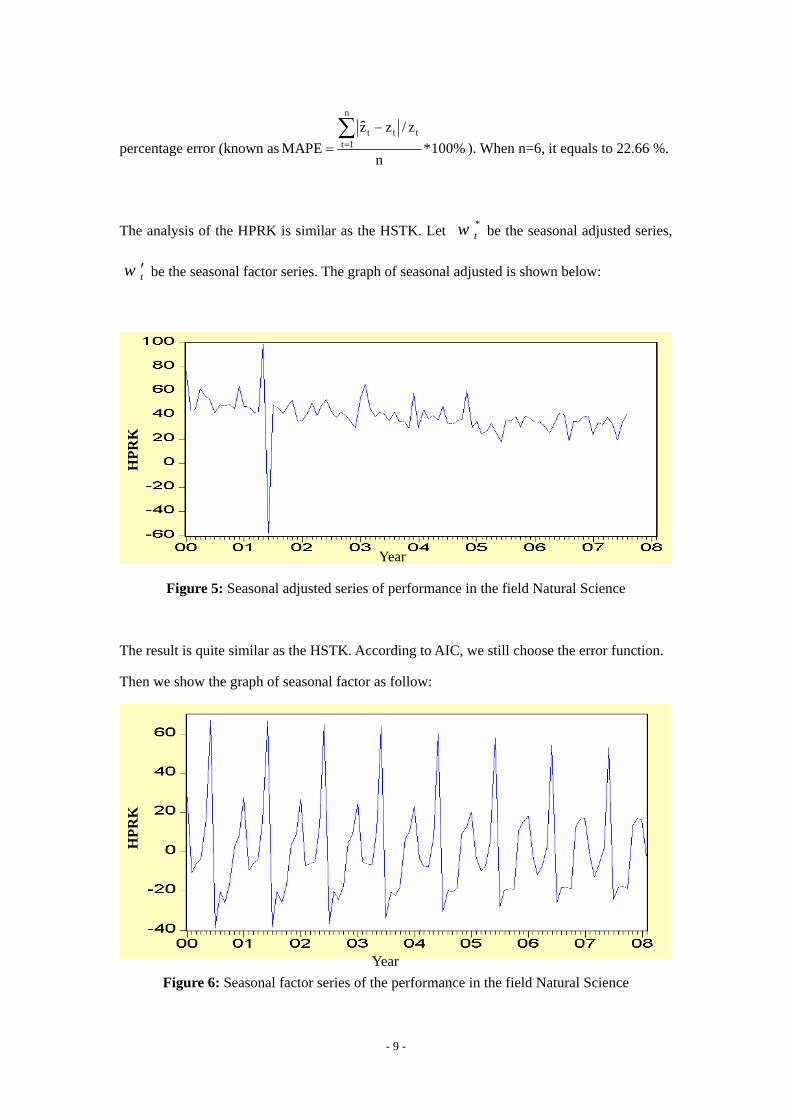
The result is quite similar as the HSTK. According to AIC, we still choose the error function.
Then we show the graph of seasonal factor as follow:
Figure 6: Seasonal factor series of the performance in the field Natural Science
HPR
K
Year
HPR
K
Year

- 10 -
According to the formulation:
*t t tˆ ˆ ˆw w w ′= + (4)
We can get the value of the tw . Figure 7 shows the linear graph of the forecasted data and the
original data.
Figure 7: Comparison between the original value and the forecasted value of the
performance in the field Natural Science
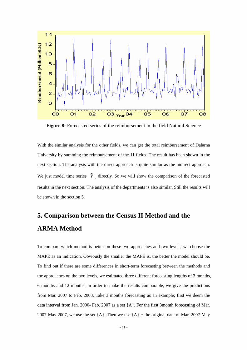
The mean absolute percentage error is 39.55 %. Then totally reimbursement of the field
Natural Science can be calculated by the function:
t 1 t 2 tˆ ˆ ˆy c * w c * z= + ( 1c 44 706= , 2c 37 702= ). Figure 8 shows the
forecasted series of the reimbursement.
HPR
K
Year
- 11 -
Figure 8: Forecasted series of the reimbursement in the field Natural Science
With the similar analysis for the other fields, we can get the total reimbursement of Dalarna
University by summing the reimbursement of the 11 fields. The result has been shown in the
next section. The analysis with the direct approach is quite similar as the indirect approach.
We just model time series ty directly. So we will show the comparison of the forecasted
results in the next section. The analysis of the departments is also similar. Still the results will
be shown in the section 5.
5. Comparison between the Census II Method and the
ARMA Method
To compare which method is better on these two approaches and two levels, we choose the
MAPE as an indication. Obviously the smaller the MAPE is, the better the model should be.
To find out if there are some differences in short-term forecasting between the methods and
the approaches on the two levels, we estimated three different forecasting lengths of 3 months,
6 months and 12 months. In order to make the results comparable, we give the predictions
from Mar. 2007 to Feb. 2008. Take 3 months forecasting as an example; first we deem the
data interval from Jan. 2000- Feb. 2007 as a set {A}. For the first 3month forecasting of Mar.
2007-May 2007, we use the set {A}. Then we use {A} + the original data of Mar. 2007-May
Rei
mbu
rsem
ent (
Mill
ion
SEK
)
Year

- 12 -
2007 to forecast the data of Jun. 2007-Aug. 2007. We use {A} + the original data of Mar.
2007-Aug. 2007 to forecast Sep. 2007-Nov. 2007. Finally, we forecast Dec. 2007-Feb. 2008
by the set {A} + the original data of Sep. 2007-Nov. 2007. After the steps above, we calculate
the MAPE of the forecasted data from Mar. 2007-Feb. 2008. The results from Census II
method are shown in the table below. We compare the results on the field level. Then we
compare results on the department level in the similar way.
Table 4: Comparison in terms of MAPE between the direct and indirect approaches with the
data classified by fields where the Census II is used for forecasting (%)
Direct Approach Indirect Approach
Period
Field
3 months 6 months 12 months 3 months 6 months 12 months
Other 42.27 48.07 48.51 42.64 49.15 50.37
Humanity 32.41 33.54 35.94 32.89 37.28 38.73
Sport 92.39 104.27 109.51 116.41 130.40 143.03
Law 30.00 38.69 43.56 34.29 40.76 45.25
Education 27.44 34.43 37.52 27.37 35.89 37.92
Media 30.52 39.48 46.50 36.07 44.72 46.86
Medicine 21.38 22.54 24.94 22.93 23.19 25.68
Natural Science 27.98 32.38 35.49 33.54 37.38 39.94
Social Science 21.95 22.45 25.08 24.25 26.97 27.35
Technique 36.02 38.68 38.85 36.27 38.21 39.94
Health Care 27.81 31.23 34.35 27.95 34.36 34.49
Average MAPE 29.78 34.15 37.07 31.82 36.79 38.65
Because the Sport field is a quite small field and the data are too few to forecast, so we can
ignore the effect it made. The Average MAPE is the average of all the fields except Sport.

- 13 -
Table 5: Comparison in terms of MAPE between the direct and indirect approaches with data
classified by departments where the Census II is used for forecasting (%)
Direct Approach Indirect Approach
Period
Department
3 months 6 months 12 months 3 months 6 months 12 months
Culture 30.60 35.87 36.51 32.60 37.32 39.94
Social 29.61 32.09 33.75 27.59 36.61 37.88
Health 27.15 32.97 35.65 29.54 33.54 37.68
Humanity 31.96 35.35 40.85 32.38 36.41 41.77
Industry 29.05 33.35 35.92 31.18 36.84 38.39
Average MAPE 29.67 33.93 36.54 30.66 36.14 39.13
From Table 4 and Table 5, on the average level, we can conclude the direct approach is better
than the indirect approach. While the data classified by departments do some help to get a
more accurate prediction than the data classified by fields. As mentioned above, in this thesis,
we also tried the ARMA model. The results are shown in tables 6 and 7:

- 14 -
Table 6: Comparison in terms of MAPE between the direct and indirect approaches with data
classified by fields where the ARMA is used for forecasting (%)
Direct Approach Indirect Approach
Period
Fields
3 months 6 months 12months 3 months 6 months 12 months
Other 38.62 44..53 46.76 41.12 45.76 49.96
Humanity 25.45 28.96 34.92 27.31 30.11 35.36
Sport 57.06 66.37 70.83 57.50 69.59 72.09
Law 32.30 41.45 44.16 36.06 41.64 45.15
Education 25.82 30.63 31.85 27.23 31.85 32.75
Media 34.04 41.36 45.59 37.04 44.19 45.33
Medicine 27.55 29.97 35.99 27.38 31.09 34.25
Natural Science 24.80 35.17 35.41 25.68 30.92 35.77
Social Science 22.10 27.27 28.52 22.99 28.51 29.44
Technique 26.38 30.68 33.88 27.47 31.62 34.84
Health Care 21.09 27.89 28.96 22.47 27.94 29.57
Average MAPE 27.82 32.60 36.60 29.48 34.36 37.24
Table 7: Comparison in terms of MAPE between the direct and indirect approaches with data
classified by departments where the ARMA is used for forecasting (%)
Direct Approach Indirect Approach
Period
Department
3 months 6 months 12 months 3 months 6 months 12 months
Culture 25.49 34.24 36.45 24.24 34.87 35.23
Social 27.29 29.90 34.66 27.08 28.78 35.02
Health 27.51 31.23 35.01 25.16 30.17 35.72
Humanity 28.06 35.15 41.26 27.80 34.60 39.07
Industry 28.19 30.81 34.67 26.89 29.02 30.26
Average MAPE 27.31 32.27 36.41 26.23 31.49 35.06

- 15 -
Compared with the table 6 and table 7, again we get the conclusion that the forecasting result
from the department level is better than the result from the field level. From the table 6, on
average, the direct approach is also better than the indirect approach as mentioned in analysis
of Census II. But it shows an opposite situation in table 7, the indirect approach achieves a
better result. Compared with Census II method, the ARMA method seems to achieve a better
result, no matter which approaches are applied to.
6. Conclusion
Judging from the rule that the smaller the MAPE is the better the forecasting result should be,
we get the conclusion that on the average level, the indirect approach with the ARMA method
and classify data on the department level achieves a better result. That is to say, to give a more
accurate forecasting reimbursement of Dalarna University we had better try this path rather
than the other paths. We analyze the reason why the ARMA model is better than the Census II
method. As we have mentioned, Census II method puts emphasis on showing trend, season,
circle and error. It decomposes the time series into these four components, but it is hard to
give an accurate decomposition for the four parts. What’s more, dealing with the data with the
moving average method for too many times may lead to the reduction of the length of the
time series. Compared with the Census II method, the ARMA method can make up these
deficiencies. In addition, ARMA method pays more weights to the recent data, which means
the forecasted result could be closer to the reality.

- 16 -
Reference
[1] Steven C. Wheelwright & Spyros Makridakis (1985), Forecasting Methods for
Management, 4TH Ed. New York: John Wiley & Sons.
[2] Walter Vandaele (1983), Applied Time Series and Box-Jenkins Models, United
States of America: Academic Press.
[3] Brockwell P. J. & Davis, R. A. (2001), Time Series: Theory and Methods,
2Ed .Beijing University Press.
[4] James Douglas. Hamilton (1994), Time Series Analysis, Princeton University
Press.
[5] Jingshui Sun (2005), Econometric, Tsinghua University Press.
[6] Shiskin J. A. H. Young & J. C. Musgrave, “The X-II Variant of the Census II
Method Seasonal Adjustment Program”, Bureau of the Census.
[7] Peter Dalgaard. (2002), Introductory Statistics with R, New York: Springer.
[8] Swedish National Agency For Higher Education: http://www.hsv.se.
- 17 -
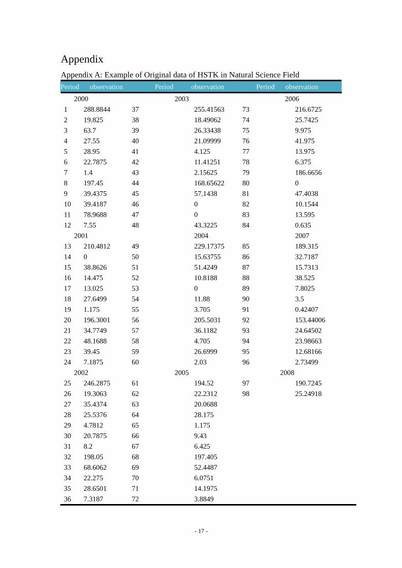
Appendix Appendix A: Example of Original data of HSTK in Natural Science Field Period observation Period observation Period observation
2000 2003 2006 1 288.8844 37 255.41563 73 216.6725 2 19.825 38 18.49062 74 25.7425 3 63.7 39 26.33438 75 9.975 4 27.55 40 21.09999 76 41.975 5 28.95 41 4.125 77 13.975 6 22.7875 42 11.41251 78 6.375 7 1.4 43 2.15625 79 186.6656 8 197.45 44 168.65622 80 0 9 39.4375 45 57.1438 81 47.4038 10 39.4187 46 0 82 10.1544 11 78.9688 47 0 83 13.595 12 7.55 48 43.3225 84 0.635 2001 2004 2007 13 210.4812 49 229.17375 85 189.315 14 0 50 15.63755 86 32.7187 15 38.8626 51 51.4249 87 15.7313 16 14.475 52 10.8188 88 38.525 17 13.025 53 0 89 7.8025 18 27.6499 54 11.88 90 3.5 19 1.175 55 3.705 91 0.42407 20 196.3001 56 205.5031 92 153.44006 21 34.7749 57 36.1182 93 24.64502 22 48.1688 58 4.705 94 23.98663 23 39.45 59 26.6999 95 12.68166 24 7.1875 60 2.03 96 2.73499 2002 2005 2008 25 246.2875 61 194.52 97 190.7245 26 19.3063 62 22.2312 98 25.24918 27 35.4374 63 20.0688 28 25.5376 64 28.175 29 4.7812 65 1.175 30 20.7875 66 9.43 31 8.2 67 6.425 32 198.05 68 197.405 33 68.6062 69 52.4487 34 22.275 70 6.0751 35 28.6501 71 14.1975 36 7.3187 72 3.8849

- 18 -
Appendix B: Example of Original data of HPRK in Natural Science Field Period observation Period observation Period observation
2000 2003 2006 1 104.0406 37 79.54375 73 52.41625 2 33.00937 38 60.18745 74 32.3225 3 38.9031 39 39.43755 75 18.83875 4 58.0988 40 31.51125 76 18.6969 5 72.0194 41 53.0612 77 36.07873 6 119.2481 42 104.4782 78 95.72749 7 2.86875 43 1.40623 79 14.1875 8 28.24687 44 21.45937 80 0 9 21.50825 45 12.3625 81 16.60688 10 31.72865 46 16.7438 82 15.61125 11 47.9399 47 35.2412 83 50.81375 12 71.6524 48 68.5662 84 55.5775 2001 2004 2007 13 74.52187 49 52.70875 85 40.69375 14 37.16873 50 41.07188 86 31.3275 15 36.3938 51 29.3675 87 19.035 16 38.34997 52 32.11625 88 31.46755 17 114.5139 53 43.29124 89 34.2912 18 9.0374 54 107.825 90 72.325 19 9.6903 55 2.4663 91 8.6517 20 25.909 56 12.7625 92 23.3783 21 15.5581 57 14.7906 93 10.6825 22 30.1125 58 17.77 94 12.2567 23 55.2988 59 68.30375 95 36.8008 24 74.52187 60 42.25375 96 45.2725 2002 2003 2008 25 43.6511 61 54.91875 97 53.09418 26 62.3115 62 22.25125 98 22.44625 27 33.4825 63 16.475 28 44.3813 64 25.54375 29 34.0987 65 30.24685 30 60.8406 66 75.6825 31 117.8094 67 8.025 32 6.4625 68 15.2913 33 17.4375 69 19.81 34 18.0813 70 11.4937 35 22.0781 71 49.8388 36 38.9832 72 52.4087

- 19 -
Appendix C: Different Reimbursement Level for Different Science Field Table A (HSTK) – registration (SEK) Field Amount Humanity HU 19 465 Sport ID 89 681 Law JU 19 465 Education LU 29 719 Medicine MD 50 875 Media ME 260 810 Natural Science NA 44 706 Social Science SA 19 465 Technique TE 44 706 Health Care VÅ 45 527 Other ÖV 35 903 Table B: (HPRK) - performance (SEK) Field Amount Humanity HU 17 085 Sport ID 42 895 Law JU 17 085 Education LU 35 385 Medicine MD 63 924 Media ME 211 087 Natural Science NA 37 702 Social Science SA 17 085 Technique TE 37 702 Health Care VÅ 40 299 Other ÖV 29 165