“SHORT-TERM EFFECTS OF STRUCTURAL REFORMS/ PAIN BEFORE THE GAIN?”:

FURTHER MATERIAL

ANNEXES TO CHAPTER 3 OF THE 2016 OECD EMPLOYMENT OUTLOOK:

EMPIRICAL METHODOLOGY, DETAILED INDICATORS AND ECONOMETRIC RESULTS

1

TABLE OF CONTENTS

ANNEX 3.A1 DEREGULATION OF BARRIERS TO ENTRY: EMPIRICAL METHODOLOGY

AND DETAILED ECONOMETRIC RESULTS ............................................................................................ 2

1. Introduction .......................................................................................................................................... 2 2. The direct effect of PMR reforms in the short-run ............................................................................... 2 3. The direct effect of PMR reforms in the long-run ................................................................................... 15 4. From direct to indirect effects: the impact of reform on industry prices ............................................ 15 5. The indirect effects of PMR reforms .................................................................................................. 16 References .................................................................................................................................................. 23

ANNEX 3.A2 REFORMS OF DISMISSAL LEGISLATION: EMPIRICAL METHODOLOGY AND

DETAILED ECONOMETRIC RESULTS ................................................................................................... 24

1. Introduction ........................................................................................................................................ 24 2. Cross-country/cross-industry/time-series analysis ............................................................................. 24 3. Regression-discontinuity models ........................................................................................................ 38 4. Difference-in-difference analysis of the 2009 Estonian reform ......................................................... 41 References .................................................................................................................................................. 45

ANNEX 3.A3 INDICATORS OF REGULATION IN PRODUCT AND LABOR MARKETS ............. 47

2

ANNEX 3.A1 DEREGULATION OF BARRIERS TO ENTRY:

EMPIRICAL METHODOLOGY AND DETAILED ECONOMETRIC RESULTS

1. Introduction

1. This Annex presents detailed explanation of the empirical methodologies adopted in the analysis

of Chapter 3, Section 1. It reports the underlying estimates, robustness tests and discusses some extensions.

2. The direct effect of PMR reforms in the short-run

2.1. Data and estimation methodology

2. The short term labor market impact of PMR reforms is estimated exploiting variation in the level

of regulation in three network industries covered by the OECD PMR database (ETCR): Energy, Transport

and Communications.1 More specifically, the analysis focuses on the sub-indexes capturing entry barriers

and vertical integration. The OECD measures, which increase in the extent of regulation and vary from

0 to 6, are available since 1975. Table 3.A3.1 reports the latest available data for OECD countries,

suggesting that regulation is still relatively high in the Energy and Transportation industries. Looking at the

time patterns of the indicators suggests that product markets have been almost exclusively subject to

deregulating reforms, with rare episodes of re-regulation (OECD 2016).2

3. Data used in the baseline sample are sourced from the EUKLEMS dataset, which covers the

period 1975-2007 and allows recovering labour market outcomes for the same 3 industries (Energy,

Transport and Communication) aggregating 2-digits industries in the ISIC rev.3 classification.3 In some

extensions, the sample is expanded to 2012 collating EUKLEMS with the most recent version of

OECD STAN.4 The analysis mainly focusses on total employment as the core dependent variable.

1 . The OECD ETCR indicators measure anti-competitive product market regulation in seven 2 or 3-digit

network sub-industries including electricity and gas (Energy), air, rail, road transport (Transport) and post

and telecommunications (Communications). For each sub-industry the dataset contains measures of

administrative entry barriers, vertical integration, the extent of public ownership, price controls and the

market share of the dominant player. Following Alesina et al. (2005) the information available in the

ETCR dataset is used to construct time-series indicators of barriers to entry for three aggregate industries

(Energy, Transport, and Communication). This method involves two steps. First, simple averages of

separate indicators of barriers to entry and vertical integration (where applicable) are taken for each of the

seven sub-industries. Second, this coarser (and partially alternative) indicator is further aggregated

(by simple averaging) at the level of the three higher-level network industries considered in the analysis.

2 . Accordingly, the analysis will not show extensions attempting to test for parameter heterogeneity between

deregulation and re-regulation episodes (as in the case of changes in EPL, see the chapter section 2) as

these tests were always non-significant.

3 . Countries in the sample include: Australia, Austria, Belgium, Canada, the Czech Republic, Denmark,

Finland, France, Germany, Greece, Hungary, Ireland, Italy, Japan, Korea, the Netherlands, Poland,

Portugal, the Slovak Republic, Spain, Sweden, the United Kingdom and the United States.

4 . OECD STAN is available for fewer but more recent years than EUKLEMS. The two dataset were

collated mapping the OECD STAN industry classification (ISIC rev.4) to the ISIC rev. 3 classification

3

This is because EUKLEMS data for wage and salary employment are not available in a consistent way for most

countries before the mid-1980s. Results are however robust to using total employment with wage and salary

employment as the dependent variable, and starting the analysis from 1985.

4. With these data at hand, a simple way to investigate this relationship is to estimate a first-difference

equation relating year-on-year employment changes in country c, industry i and time t (∆𝐸𝑐𝑖𝑡 = 𝑙𝑛𝐿𝑐𝑖𝑡 −𝑙𝑛𝐿𝑐𝑖𝑡−1) to regulatory reforms as in:

∆𝐸𝑐𝑖𝑡 = 𝛽0∆𝐵𝐸𝑐𝑖𝑡 + 𝑋𝑐𝑖𝑡𝛾 + 𝐷𝑐𝑡 + 𝐷𝑖𝑡 + 𝐷𝑐𝑖 + 휀𝑐𝑖𝑡 (1)

where ∆𝐵𝐸𝑐𝑖𝑡is the change in the OECD regulation index (if any) traceable to reforms lowering entry barriers

and/or vertical integration in the corresponding industry; ε is an error term.5 The vector X accounts for the

potentially confounding role of other forms of industry regulation (i.e. the extent of public ownership) or the

burden of barriers to entry in other industries. The set of bi-dimensional fixed-effects Dct, Dit and Dci aims to

capture, respectively: i) country-specific shocks to employment growth common to all industries (e.g. the business

cycle and economy-wide policy reforms); ii) industry-specific shocks to employment growth common across

countries (such as those related to the evolution of technology and global demand); and iii) country-industry

specific linear trends in the evolution of employment (e.g. due to changes in the long-run patterns of international

specialisation).

5. Absent spillover effects of deregulation across industries (see next paragraph), equation (1) would allow

estimating the contemporaneous impact of regulatory reforms on employment changes. A positive estimated β0

would suggest that, for example, lower regulation in industry i is associated with lower own-industry employment.

However, any omitted factor driving both changes in employment and changes in regulation is likely to bias OLS

estimates of β0. For example, industry-specific liberalisation reforms might be more easily undertaken when the

industry faces a significant crisis. Alternatively, deregulation might be less resisted by trade unions when industry

employment is on the rise, and organisational changes following deregulation are less likely to threaten the jobs of

insiders. One way to account for these concerns consists in looking at the effect of lagged values of the variable of

interest. Moreover, one would like to account for possible persistence of employment changes, accounting for

lagged values of the dependent variable. This leads to a dynamic version of (1):

∆𝐸𝑐𝑖𝑡 = 𝛽0∆𝐵𝐸𝑐𝑖𝑡 + ∑ (𝛽𝑘∆𝐵𝐸𝑐𝑖𝑡−𝑘 + 𝛿𝑘∆𝐸𝑐𝑖𝑡−𝑘)𝑇𝑘=1 + 𝑋𝑐𝑖𝑡𝛾 + 𝐷𝑐𝑡 + 𝐷𝑖𝑡 + 𝐷𝑐𝑖 + 휀𝑐𝑖𝑡 (2)

with the number of lags defined on the basis of some statistical criterion such as the Bayesian’s BIC or Akaike’s

AIC.6 Note that, if the parameters 𝛿𝑘 are not of interest the equation (2) can be rewritten by substituting recursively

all terms of the lagged dependent variable, leading to an infinite series of ∆𝐵𝐸 terms on the right-hand side (see

e.g. Teulings and Zubanov, 2014). This would allow addressing the fact that, as shown by Nickell (1981), the

coefficients of the lagged dependent variable in equations (2) are usually biased, and might yield biased estimates

(used by EUKLEMS). The mapping was obtained using 3-digit level employment data from EU LFS and

tested on years for which both classifications are available, but remains nonetheless imperfect.

Accordingly, the resulting sample is only used in sensitivity analysis (rather than as the preferred dataset).

This is because breaks in the industry classification can severely alter the estimated short-run dynamics and

measurement error induce biases in the estimated parameters.

5 . To account for serial correlation in the residual, standard errors are clustered

at the country-by-industry level.

6 . The contemporaneous term is included as it allows capturing systematic shocks that are simultaneous to the

dependent variable (in particular shocks to the variable of interest) whose omission might lead to biased

coefficients (Teulings and Zubanov, 2014).

4

of the coefficients of interest if covariates are correlated.7 To check the relevance of the estimation concerns

discussed above, this annex will present evidence from all the above mentioned specifications.

6. Conditional on this large set of controls, identification hinges on comparing employment growth

in the reformed industry in a given year to growth in the other industries (or to growth in the same industry,

over time). The former, however, might not be a valid counterfactual if there are spillover effects from

reforms in one industry to employment in the other two industries. For example, if deregulating the energy

market affects input choices and thus employment dynamics in the transport industry; in that case

employment growth in transports would not represent a valid counterfactual for the “no-reform” scenario

in energy. To check for the relevance of cross-industry spillovers, the baseline specification has been

augmented with the average change in regulation in “other” network industries. (The results suggest these

effects are negligible).

7. All in all, the estimated coefficients would not be interpretable as the aggregate impact

of deregulation on employment in presence of country-industry shocks to employment growth that are

neither common to all other industries in the country, nor shared with the same industry across countries,

nor captured by long term country-specific industry trends, nor reflecting cross-industry spillover effects,

and yet are systematically correlated with PMR deregulation. Even if these confounding factors can

plausibly be excluded, deregulation policies might be a consequence (not the source) of employment

shocks; accordingly the analysis also performs alternative tests of reverse-causality. One consists in

including forward terms of regulation: finding that future regulation affects current employment would

provide evidence of reverse causality. Granger-causality tests are also performed, which amount to

regressing the change in regulation at time t (ΔBE) on two lags of employment changes, and testing that

the latter have no individual or cumulative impact.8

8. This setting allows for several important extensions of the empirical specification. First, it allows

checking the relevance of other dimensions of regulation accounting, for example, for changes in the extent

of state controls (public ownership) to distinguish the effects of deregulation from those of privatization.

Second, one can check for industry-specific intensities in the employment impact of regulatory reforms

allowing for heterogeneous parameter estimates. Third, the specification allows examining heterogeneity in

the impact of deregulation over the business cycle, which has potential implications for the optimal timing

of this type of structural reforms. To this purpose, the change in regulation ΔBE is interacted with the

change in the output gap as measured from the OECD EO database. The output gap (OG) is defined as the

difference between current and potential output, so that ΔOG takes negative values when the economy is in

a downturn. Hence, a negative sign on this interaction would suggest that the short-run employment costs

from deregulation are aggravated by worsening economic conditions and attenuated in upswings.

7 . The specification would become ∆𝐸𝑐𝑖𝑡 = ∑ 𝛽𝑘∆𝐵𝐸𝑐𝑖𝑡−𝑘M𝑘=0 + 𝑋𝑐𝑖𝑡𝛾 + 𝐷𝑐𝑡 + 𝐷𝑖𝑡 + 𝐷𝑐𝑖 + 휀𝑐𝑖𝑡, with again M

set on the basis of BIC or AIC statistics (which would usually lead to M > T).

8 . An alternative approach would be to use instrumental variables. Bassanini (2015) use political variables as

instruments for deregulation obtaining results that are consistent with those presented here.

5

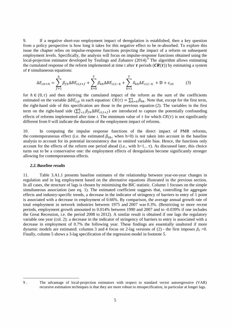
9. If a negative short-run employment impact of deregulation is established, then a key question

from a policy perspective is how long it takes for this negative effect to be re-absorbed. To explore this

issue the chapter relies on impulse-response functions projecting the impact of a reform on subsequent

employment levels. Specifically, the analysis will focus on impulse-response functions obtained using the

local-projection estimator developed by Teulings and Zubanov (2014).9 The algorithm allows estimating

the cumulated response of the reform implemented at time t after 𝝉 periods (𝑪𝑹(𝝉)) by estimating a system

of 𝝉 simultaneous equations:

∆𝐸𝑐𝑖𝑡+ℎ = ∑ 𝛽𝑓ℎ∆𝐵𝐸𝑐𝑖,𝑡+𝑓

ℎ

𝑓=1

+ ∑ 𝛽𝑘ℎ∆𝐵𝐸𝑐𝑖,𝑡−𝑘

𝑇

𝑘=0

+ ∑ 𝛿𝑘ℎ∆𝐸𝑐𝑖,𝑡−𝑘

𝑇

𝑘=1

+ 𝔻 + 휀𝑐𝑖𝑡 (3)

for ℎ ∈ (0, 𝜏) and then deriving the cumulated impact of the reform as the sum of the coefficients

estimated on the variable ∆𝐵𝐸𝑐𝑗𝑡 in each equation: 𝐶𝑅(𝜏) = ∑ 𝛽0ℎ𝜏ℎ=0 . Note that, except for the first term,

the right-hand side of this specification are those in the previous equation (2). The variables in the first

term on the right-hand side (∑ 𝛽𝑓ℎ∆𝐵𝐸𝑐𝑖,𝑡+𝑓ℎ𝑓=1 ) are introduced to capture the potentially confounding

effects of reforms implemented after time t. The minimum value of 𝜏 for which 𝐶𝑅(𝜏) is not significantly

different from 0 will indicate the duration of the employment impact of reforms.

10. In computing the impulse response functions of the direct impact of PMR reforms,

the contemporaneous effect (i.e. the estimated 𝛽0ℎ, when h=0) is not taken into account in the baseline

analysis to account for its potential inconsistency due to omitted variable bias. Hence, the functions only

account for the effects of the reform one period ahead (i.e., with h=1... 𝜏). As discussed later, this choice

turns out to be a conservative one: the employment effects of deregulation become significantly stronger

allowing for contemporaneous effects.

2.2. Baseline results

11. Table 3.A1.1 presents baseline estimates of the relationship between year-on-year changes in

regulation and in log employment based on the alternative equations illustrated in the previous section.

In all cases, the structure of lags is chosen by minimising the BIC statistic. Column 1 focuses on the simple

simultaneous association (see eq. 1). The estimated coefficient suggests that, controlling for aggregate

effects and industry-specific trends, a decrease in the indicator of stringency of barriers to entry of 1 point

is associated with a decrease in employment of 0.66%. By comparison, the average annual growth rate of

total employment in network industries between 1975 and 2007 was 0.3%. (Restricting to more recent

periods, employment growth amounted to 0.014% between 1990 and 2007 and to -0.039% if one includes

the Great Recession, i.e. the period 2008 to 2012). A similar result is obtained if one lags the regulatory

variable one year (col. 2): a decrease in the indicator of stringency of barriers to entry is associated with a

decrease in employment of 0.7% the following year. These findings are essentially unaltered if more

dynamic models are estimated: columns 3 and 4 focus on 2-lag versions of (2) - the first imposes β0 =0.

Finally, column 5 shows a 3-lag specification of the regression model in footnote 5.

9 . The advantage of local-projection estimators with respect to standard vector autoregressive (VAR)

recursive estimation techniques is that they are more robust to misspecification, in particular at longer lags.

6

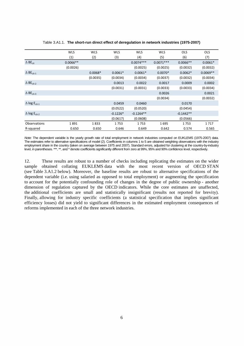
Table 3.A1.1. The short-run direct effect of deregulation in network industries (1975-2007)

Note: The dependent variable is the yearly growth rate of total employment in network industries computed on EUKLEMS (1975-2007) data. The estimates refer to alternative specifications of model (2). Coefficients in columns 1 to 5 are obtained weighting observations with the industry employment share in the country (taken on average between 1975 and 2007). Standard errors, adjusted for clustering at the country-by-industry level, in parentheses. ***, **, and * denote coefficients significantly different from zero at 99%, 95% and 90% confidence level, respectively.

12. These results are robust to a number of checks including replicating the estimates on the wider

sample obtained collating EUKLEMS data with the most recent version of OECD STAN

(see Table 3.A1.2 below). Moreover, the baseline results are robust to alternative specifications of the

dependent variable (i.e. using salaried as opposed to total employment) or augmenting the specification

to account for the potentially confounding role of changes in the degree of public ownership - another

dimension of regulation captured by the OECD indicators. While the core estimates are unaffected,

the additional coefficients are small and statistically insignificant (results not reported for brevity).

Finally, allowing for industry specific coefficients (a statistical specification that implies significant

efficiency losses) did not yield to significant differences in the estimated employment consequences of

reforms implemented in each of the three network industries.

WLS WLS WLS WLS WLS OLS OLS

(1) (2) (3) (4) (5) (6) (7)

D BEcit 0.0066** 0.0074*** 0.0071*** 0.0066** 0.0061*

(0.0026) (0.0025) (0.0025) (0.0032) (0.0032)

D BEcit-1 0.0068* 0.0061* 0.0061* 0.0070* 0.0062* 0.0069**

(0.0035) (0.0034) (0.0034) (0.0037) (0.0032) (0.0034)

D BEcit-2 0.0013 0.0022 0.0017 0.0009 0.0002

(0.0031) (0.0031) (0.0033) (0.0033) (0.0034)

D BEcit-3 0.0026 0.0021

(0.0034) (0.0032)

D log Ecit-1 0.0459 0.0460 0.0170

(0.0522) (0.0520) (0.0454)

D log Ecit-2 -0.1226* -0.1264** -0.1442**

(0.0617) (0.0608) (0.0566)

Observations 1 891 1 833 1 753 1 753 1 695 1 753 1 717

R-squared 0.650 0.650 0.646 0.649 0.642 0.574 0.565

7

Table 3.A1.2. The short-run direct effect of deregulation in network industries (1975-2012)

Note: The dependent variable is the yearly growth rate of total employment in network industries computed on a sample obtained collating EUKLEMS and STAN data (1975-2012). The estimates refer to alternative specifications of model (2). Coefficients in columns 1 to 5 are obtained weighting observations with the industry employment share in the country (taken on average between 1975 and 2007). Standard errors, adjusted for clustering at the country-by-industry level, in parentheses. ***, **, and * denote coefficients significantly different from zero at 99%, 95% and 90% confidence level, respectively.

13. As discussed in the previous section, these estimates might be biased if policy responds to

changes in industry employment. The direction of the bias is not obvious. In fact, while on the one hand a

sequence of negative shock (e.g. a crisis) might facilitate industry reform, on the other hand

industry-specific lobbies could put pressure to postpone them. In order to address these issues, the models

in Table 3.A1.1 are re-estimated including one forward term – that is the change in regulation in the

following year (∆𝐵𝐸𝑐𝑖,𝑡+1). If policy-makers react with some delay to employment changes, one would

expect this term to be significant (and the estimated effect of reforms to be affected). The results reported

in Table 3.A1.3, however, do not support this hypothesis.

Table 3.A1.3. Robustness to including forward terms

Note: The dependent variable is the yearly growth rate of total employment in network industries computed on EUKLEMS data.

The estimates are obtained augmenting the specifications in Table 3.A1.1 with a forward term (∆𝐵𝐸𝑐𝑖,𝑡+1). Coefficients in columns 1 to

5 are obtained weighting observations with the industry employment share in the country (taken on average between 1975 and 2007). Standard errors, adjusted for clustering at the country-by-industry level, in parentheses. ***, **, and * denote coefficients significantly different from zero at 99%, 95% and 90% confidence level, respectively.

WLS WLS WLS WLS WLS OLS OLS

(1) (2) (3) (4) (5) (6) (7)

D BEcit 0.0059** 0.0067*** 0.0062** 0.0061* 0.0055*

(0.0025) (0.0025) (0.0025) (0.0031) (0.0031)

D BEcit-1 0.0067* 0.0065* 0.0064* 0.0070* 0.0064* 0.0069*

(0.0036) (0.0035) (0.0036) (0.0038) (0.0033) (0.0035)

D BEcit-2 0.0020 0.0027 0.0020 0.0017 0.0009

(0.0030) (0.0029) (0.0032) (0.0032) (0.0033)

D BEcit-3 0.0042 0.0034

(0.0036) (0.0034)

D log Ecit-1 0.0459 0.0460 0.0190

(0.0622) (0.0616) (0.0527)

D log Ecit-2 -0.1126* -0.1154* -0.1388**

(0.0630) (0.0625) (0.0569)

Observations 2 012 1 962 1 877 1 876 1 849 1 876 1 849

R-squared 0.629 0.628 0.623 0.624 0.618 0.557 0.551

WLS WLS WLS WLS WLS OLS OLS

(1) (2) (3) (4) (5) (6) (7)

D BEcit 0.0067** 0.0074*** 0.0072*** 0.0066** 0.0061*

(0.0026) (0.0026) (0.0026) (0.0032) (0.0033)

D BEcit-1 0.0066* 0.0057* 0.0057* 0.0068* 0.0057* 0.0065*

(0.0033) (0.0032) (0.0033) (0.0035) (0.0032) (0.0034)

D BEcit+1 -0.0006 0.0002 -0.0001 -0.0000 0.0007 -0.0013 -0.0011

(0.0031) (0.0031) (0.0029) (0.0029) (0.0030) (0.0028) (0.0030)

Observations 1 822 1 764 1 684 1 684 1 626 1 699 1 663

R-squared 0.654 0.654 0.649 0.652 0.645 0.576 0.568

8

14. A more formal (“Granger-causality”) test is presented in Table 3.A1.4. The idea is to test whether

past changes in employment affect the change in barriers to entry today, estimating a model similar to (1)

but with ∆𝐵𝐸as the dependent variable: ∆𝐵𝐸𝑐𝑖𝑡 = ∑ 𝜋𝑘∆𝐸𝑐𝑖,𝑡−𝑘2𝑘=0 + ∑ 𝜑𝑙∆𝐵𝐸𝑐𝑖,𝑡−𝑙

2𝑙=1 + 𝔻 + 𝜔𝑐𝑖𝑡.

The table reports the values of F-tests for the significance of 𝜋1 and 𝜋2, both separately and cumulatively.

Consistent with the previous findings, past employment changes do not have a significant impact on

current changes in regulation (neither separately nor cumulatively).

Table 3.A1.4 Granger-causality tests of reverse causality

Note: The table presents F-tests of the coefficients of the first two lags of employment growth (∆𝐸𝑐𝑖,𝑡−1and ∆𝐸𝑐𝑖,𝑡−2) in models where

the change in Barriers to entry (∆𝐵𝐸𝑐𝑖𝑡) is the dependent variable. The full specification also includes two lags of D, country-by-industry, country-by-time and industry-by-time dummies. “F-test, cumulative impact” is for the F-test on the sum of both

lagged D log Employment coefficients. F-statistics are distributed as F(1,68) under the null (test statistics are obtained by clustering errors at the country-by-industry level). None of the reported statistics is significant at standard levels.

15. To check for the relevance of potential cross-industry spillovers the baseline specification has

been augmented with the average change in regulation in “other” network industries. Specifically, the

specification is augmented with the first difference of the term: 𝑊𝐵𝐸𝑑𝑖𝑡 = ∑ 𝐸𝑥𝑝𝑖,−𝑖 ∗ 𝐵𝐸𝑐,−𝑖,𝑡−𝑖 , where

Expi,-i are coefficients from the US Inverse Leontief Matrix measuring how many units of input -i have to

be produced (at any stage of the value chain) to produce one additional unit for final demand in network

industry i. Hence 𝑊𝐵𝐸𝑑𝑖𝑡 captures the impact on employment in network industry i of regulatory reforms

implemented in the other two industries. If spillovers were an important driver of industry employment

dynamics, this control should attract a significant coefficient. However, the results (not reported for

brevity) suggest spillover effects are negligible. For example, augmenting specifications in columns 1 and

4 with the appropriate (i.e. contemporaneous and lagged) values of 𝑊𝐵𝐸𝑑𝑖𝑡 did not yield to estimate

statistically significant coefficients on the latter at standard levels of acceptance. By contrast, the

coefficients on own-deregulation (variables ∆𝐵𝐸𝑐,𝑖,𝑡) were unaffected (if anything, slightly larger).

16. The analysis also explored whether the strength of a given reform varies with the level of

regulation. This was obtained interacting the change in the OECD regulation index (∆𝐵𝐸𝑐𝑖) with a dummy

variable 𝐻𝑅𝑐𝑖𝑡−1 indicating whether average regulation in each network industry in country c was above or

below the sample median the year before the reform. Throughout the core specifications 1, 2 and 4 of Table

3.A1.1 the interaction term attracted a non-statistically significant coefficient, providing no evidence that

the impact of pro-competitive reforms is non-linear in initial regulation (e.g. stronger in high than low

regulated countries).

2.3. Heterogeneous effects over the business-cycle

17. The previous results show that deregulation of entry in network industries induces higher initial

job destruction than job creation, resulting in a net short-term employment contraction. Do these effects

vary between economic downturns and upturns? To shed light on these issues, the baseline specification is

augmented with the interaction between changes in entry barriers and changes in the contemporaneous

output gap (OG). The output gap is defined as the difference between current and potential output, so its

Not including Including

D log Employment (t ) D log Employment (t )

(1) (2)

F-test on D log Employment (t -1) 0.19 0.2

F-test on D log Employment (t -2) 2.39 1.94

F-test, cumulative impact 0.54 0.38

9

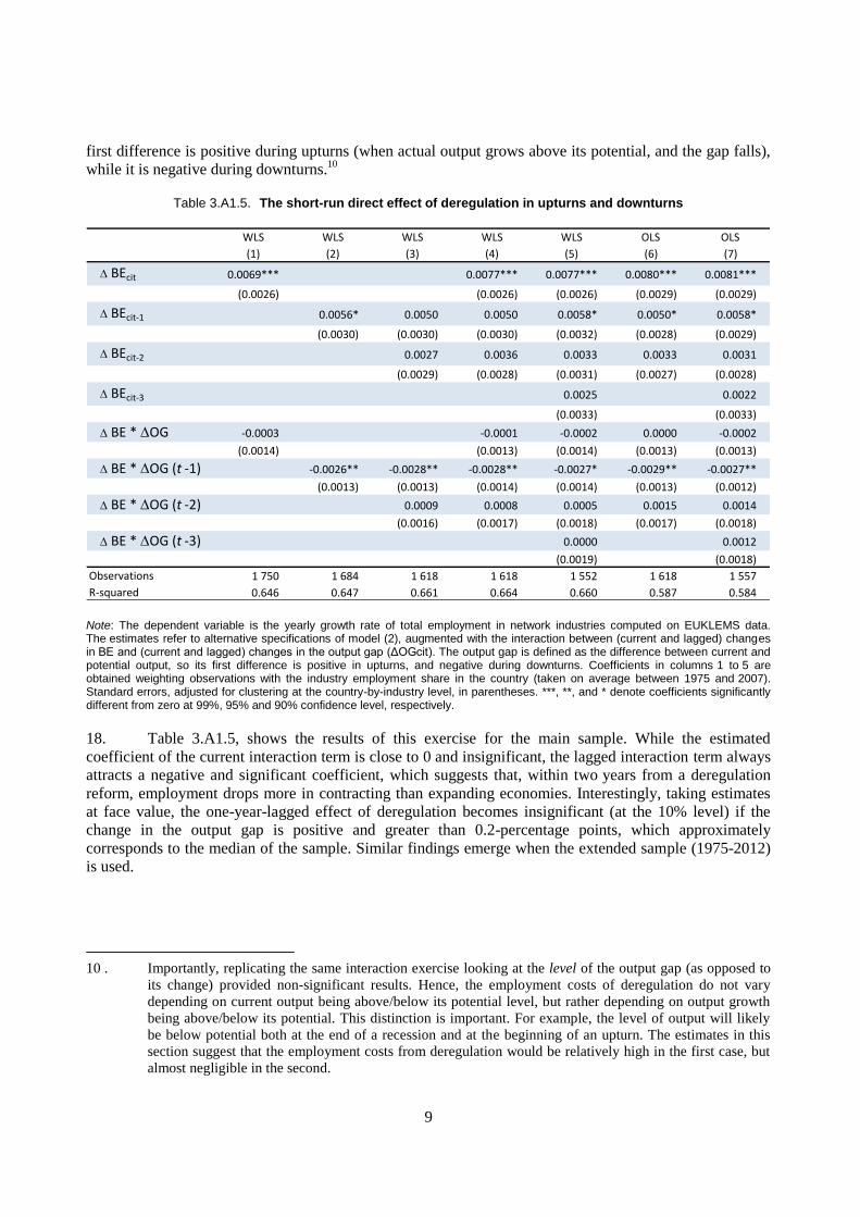
first difference is positive during upturns (when actual output grows above its potential, and the gap falls),

while it is negative during downturns.10

Table 3.A1.5. The short-run direct effect of deregulation in upturns and downturns

Note: The dependent variable is the yearly growth rate of total employment in network industries computed on EUKLEMS data. The estimates refer to alternative specifications of model (2), augmented with the interaction between (current and lagged) changes in BE and (current and lagged) changes in the output gap (ΔOGcit). The output gap is defined as the difference between current and potential output, so its first difference is positive in upturns, and negative during downturns. Coefficients in columns 1 to 5 are obtained weighting observations with the industry employment share in the country (taken on average between 1975 and 2007). Standard errors, adjusted for clustering at the country-by-industry level, in parentheses. ***, **, and * denote coefficients significantly different from zero at 99%, 95% and 90% confidence level, respectively.

18. Table 3.A1.5, shows the results of this exercise for the main sample. While the estimated

coefficient of the current interaction term is close to 0 and insignificant, the lagged interaction term always

attracts a negative and significant coefficient, which suggests that, within two years from a deregulation

reform, employment drops more in contracting than expanding economies. Interestingly, taking estimates

at face value, the one-year-lagged effect of deregulation becomes insignificant (at the 10% level) if the

change in the output gap is positive and greater than 0.2-percentage points, which approximately

corresponds to the median of the sample. Similar findings emerge when the extended sample (1975-2012)

is used.

10 . Importantly, replicating the same interaction exercise looking at the level of the output gap (as opposed to

its change) provided non-significant results. Hence, the employment costs of deregulation do not vary

depending on current output being above/below its potential level, but rather depending on output growth

being above/below its potential. This distinction is important. For example, the level of output will likely

be below potential both at the end of a recession and at the beginning of an upturn. The estimates in this

section suggest that the employment costs from deregulation would be relatively high in the first case, but

almost negligible in the second.

WLS WLS WLS WLS WLS OLS OLS

(1) (2) (3) (4) (5) (6) (7)

D BEcit 0.0069*** 0.0077*** 0.0077*** 0.0080*** 0.0081***

(0.0026) (0.0026) (0.0026) (0.0029) (0.0029)

D BEcit-1 0.0056* 0.0050 0.0050 0.0058* 0.0050* 0.0058*

(0.0030) (0.0030) (0.0030) (0.0032) (0.0028) (0.0029)

D BEcit-2 0.0027 0.0036 0.0033 0.0033 0.0031

(0.0029) (0.0028) (0.0031) (0.0027) (0.0028)

D BEcit-3 0.0025 0.0022

(0.0033) (0.0033)

D BE * DOG -0.0003 -0.0001 -0.0002 0.0000 -0.0002

(0.0014) (0.0013) (0.0014) (0.0013) (0.0013)

D BE * DOG (t -1) -0.0026** -0.0028** -0.0028** -0.0027* -0.0029** -0.0027**

(0.0013) (0.0013) (0.0014) (0.0014) (0.0013) (0.0012)

D BE * DOG (t -2) 0.0009 0.0008 0.0005 0.0015 0.0014

(0.0016) (0.0017) (0.0018) (0.0017) (0.0018)

D BE * DOG (t -3) 0.0000 0.0012

(0.0019) (0.0018)

Observations 1 750 1 684 1 618 1 618 1 552 1 618 1 557

R-squared 0.646 0.647 0.661 0.664 0.660 0.587 0.584

10

2.4. Impulse-response functions

19. How long does it take for the initial negative employment effect of deregulation to be reverted?

A set of impulse response functions estimated using local-projection estimators à la Teulings and Zubanov

helps answering this question (Figure 3.A1.1). Panels A and C are based on the coefficients estimated

in columns 4 and 6 of Table 3.A1.1 (referring to weighted and unweighted estimates, respectively, in the

baseline sample). Panels B and D are based on the same columns of Table 3.A1.2 (weighted

and unweighted estimates in the extended sample). Both figures show that the cumulated impact

on industry employment remains significant for the first three periods. At lag 4, the cumulated impact is

somewhat below the initial effect and insignificantly different from zero (partly due to the lower precision

of the corresponding estimate).

Figure 3.A1.1. Competition-enhancing reforms and employment in network industries

Estimated cumulated change in industry employment up to four years since the reform, in percentage

Note: The chart reports point estimates and 90%-confidence intervals of the cumulated employment effect of PMR reforms lowering entry barriers. Estimates refer to the case of a reform lowering the OECD indicator of PMR in network industries (Energy, Transport and Communication, ETCR) by one point. Employment levels before the reform are normalised to 0. The underlying parameters are estimated allowing employment growth in each network industry to depend on lagged values of industry regulation as well as on

-3

-2.5

-2

-1.5

-1

-0.5

0

0.5

1

Before 1 2 3 4

Time since reform (years)

A. Weighted regression, 1975-2007

-3

-2.5

-2

-1.5

-1

-0.5

0

0.5

1

Before 1 2 3 4

Time since reform (years)

B. Weighted regression, 1975-2012

-3

-2.5

-2

-1.5

-1

-0.5

0

0.5

1

Before 1 2 3 4

Time since reform (years)

C. Unweighted regression, 1975-2007

-3

-2.5

-2

-1.5

-1

-0.5

0

0.5

1

Before 1 2 3 4

Time since reform (years)

D. Unweighted regression, 1975-2012

11

lagged employment changes. Confidence intervals are obtained by clustering errors on countries and industries. The four charts corresponded to different estimation methods and underling sample. Panel A uses coefficients from weighted regression in the EUKLEMS sample (1975-2007). Panel B uses coefficients from weighted regression in the combined EUKLEMS-STAN sample (1975-2012). Panels C and D use unweighted regression coefficients from the same samples. Confidence intervals are obtained by clustering errors on countries and industries.

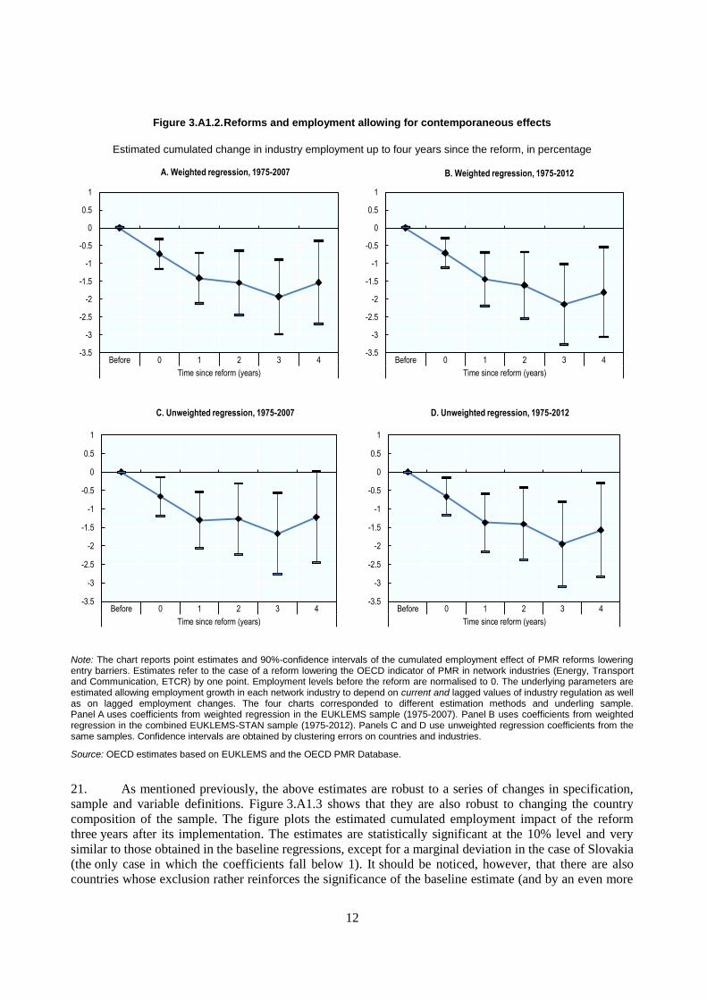
20. The above responses are plotted without factoring in the contemporaneous effect of changes in

barriers to entry, a conservative assumption motivated by the uncertainty on the reliability of

parameter 𝛽0ℎ. Considers the contribution of all estimated 𝛽s, as done in Figure 3.A1.2, would deliver

stronger effects. For example, the aggregate employment fall in the baseline regression would amount to

nearly 2% (as opposed to 1.14%) three years after the reform.

12

Figure 3.A1.2. Reforms and employment allowing for contemporaneous effects

Estimated cumulated change in industry employment up to four years since the reform, in percentage

Note: The chart reports point estimates and 90%-confidence intervals of the cumulated employment effect of PMR reforms lowering entry barriers. Estimates refer to the case of a reform lowering the OECD indicator of PMR in network industries (Energy, Transport and Communication, ETCR) by one point. Employment levels before the reform are normalised to 0. The underlying parameters are estimated allowing employment growth in each network industry to depend on current and lagged values of industry regulation as well as on lagged employment changes. The four charts corresponded to different estimation methods and underling sample. Panel A uses coefficients from weighted regression in the EUKLEMS sample (1975-2007). Panel B uses coefficients from weighted regression in the combined EUKLEMS-STAN sample (1975-2012). Panels C and D use unweighted regression coefficients from the same samples. Confidence intervals are obtained by clustering errors on countries and industries.

Source: OECD estimates based on EUKLEMS and the OECD PMR Database.

21. As mentioned previously, the above estimates are robust to a series of changes in specification,

sample and variable definitions. Figure 3.A1.3 shows that they are also robust to changing the country

composition of the sample. The figure plots the estimated cumulated employment impact of the reform

three years after its implementation. The estimates are statistically significant at the 10% level and very

similar to those obtained in the baseline regressions, except for a marginal deviation in the case of Slovakia

(the only case in which the coefficients fall below 1). It should be noticed, however, that there are also

countries whose exclusion rather reinforces the significance of the baseline estimate (and by an even more

-3.5

-3

-2.5

-2

-1.5

-1

-0.5

0

0.5

1

Before 0 1 2 3 4

Time since reform (years)

A. Weighted regression, 1975-2007

-3.5

-3

-2.5

-2

-1.5

-1

-0.5

0

0.5

1

Before 0 1 2 3 4

Time since reform (years)

B. Weighted regression, 1975-2012

-3.5

-3

-2.5

-2

-1.5

-1

-0.5

0

0.5

1

Before 0 1 2 3 4

Time since reform (years)

C. Unweighted regression, 1975-2007

-3.5

-3

-2.5

-2

-1.5

-1

-0.5

0

0.5

1

Before 0 1 2 3 4

Time since reform (years)

D. Unweighted regression, 1975-2012

13

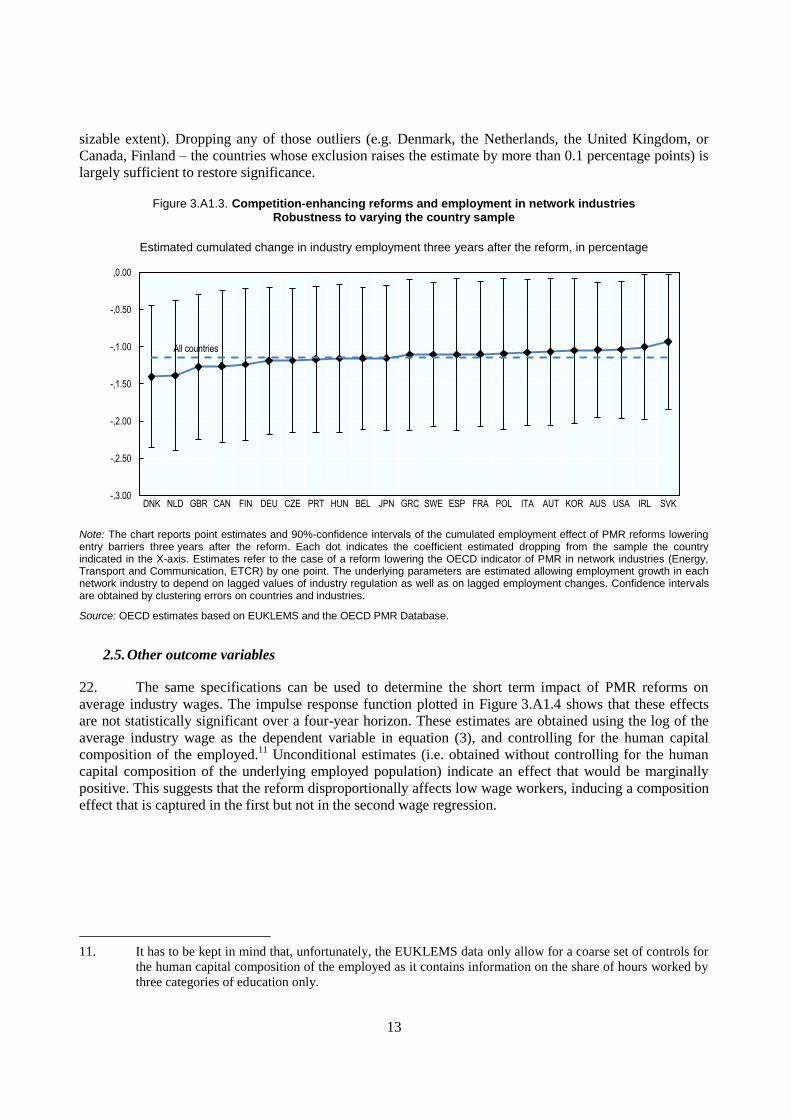
sizable extent). Dropping any of those outliers (e.g. Denmark, the Netherlands, the United Kingdom, or

Canada, Finland – the countries whose exclusion raises the estimate by more than 0.1 percentage points) is

largely sufficient to restore significance.

Figure 3.A1.3. Competition-enhancing reforms and employment in network industries Robustness to varying the country sample

Estimated cumulated change in industry employment three years after the reform, in percentage

Note: The chart reports point estimates and 90%-confidence intervals of the cumulated employment effect of PMR reforms lowering entry barriers three years after the reform. Each dot indicates the coefficient estimated dropping from the sample the country indicated in the X-axis. Estimates refer to the case of a reform lowering the OECD indicator of PMR in network industries (Energy, Transport and Communication, ETCR) by one point. The underlying parameters are estimated allowing employment growth in each network industry to depend on lagged values of industry regulation as well as on lagged employment changes. Confidence intervals are obtained by clustering errors on countries and industries.

Source: OECD estimates based on EUKLEMS and the OECD PMR Database.

2.5. Other outcome variables

22. The same specifications can be used to determine the short term impact of PMR reforms on

average industry wages. The impulse response function plotted in Figure 3.A1.4 shows that these effects

are not statistically significant over a four-year horizon. These estimates are obtained using the log of the

average industry wage as the dependent variable in equation (3), and controlling for the human capital

composition of the employed.11

Unconditional estimates (i.e. obtained without controlling for the human

capital composition of the underlying employed population) indicate an effect that would be marginally

positive. This suggests that the reform disproportionally affects low wage workers, inducing a composition

effect that is captured in the first but not in the second wage regression.

11. It has to be kept in mind that, unfortunately, the EUKLEMS data only allow for a coarse set of controls for

the human capital composition of the employed as it contains information on the share of hours worked by

three categories of education only.

-,3.00

-,2.50

-,2.00

-,1.50

-,1.00

-,0.50

,0.00

DNK NLD GBR CAN FIN DEU CZE PRT HUN BEL JPN GRC SWE ESP FRA POL ITA AUT KOR AUS USA IRL SVK

All countries

14

Figure 3.A1.4. Competition-enhancing reforms and wages in network industries

Estimated cumulated change in industry wages up to four years since the reform, in percentage

Note: The chart reports point estimates and 90%-confidence intervals of the cumulated wage effect of PMR reforms lowering entry barriers. Estimates refer to the case of a reform lowering the OECD indicator of PMR in network industries (Energy, Transport and Communication, ETCR) by one point. Employment levels before the reform are normalised to 0. The underlying parameters are estimated allowing employment growth in each network industry to depend on lagged values of industry regulation as well as on lagged employment changes. Figures reported in Panel B are obtained from a specification controlling for changes in employment and the share of the low-educated in total hours worked. Confidence intervals are obtained by clustering errors on countries and industries.

Source: OECD estimates based on EUKLEMS and the OECD PMR Database.

-1

-0.5

0

0.5

1

1.5

2

2.5

3

3.5

Before 1 2 3 4

Time since reform (years)

A. Without correcting for composition effects

-1.5

-1

-0.5

0

0.5

1

1.5

2

2.5

Before 1 2 3 4

Time since reform (years)

B. Correcting for composition effects

15

3. The direct effect of PMR reforms in the long-run

23. The longer term consequences of service deregulation on own-industry employment and wages are

estimated in a static panel setting:

𝐸𝑐𝑖𝑡 = 𝛽𝐿𝑅𝐵𝐸𝑐𝑖𝑡 + 𝜂𝑐𝑡 + 𝜂𝑗𝑡 + 𝜂𝑐𝑗 + 𝜖𝑐𝑗𝑡 (4)

where 𝐸𝑐𝑖𝑡 is the (log of) employment in country c, industry j and time t, and BEcit is the level of regulation

(entry barriers). In this framework, the set of bi-dimensional fixed-effects aim at capturing

i) employment shocks common to all industries in a country (including the country’s economic conditions,

institutions, policies etc), ii) industry-specific shocks to employment that are common across countries

(such as those related to the evolution of technology and global demand) and iii) time invariant

country-industry specific determinants of employment (e.g. linked to endowments, comparative

advantages, etc.). Serial correlation, that is the correlation between error terms for a given country-industry

cj over time, is accounted for by appropriately clustering the standard errors (but observations are still

assumed to be independent across clusters).12

24. The first four columns of Table 3.A1.6 show that estimating equation (4) using alternative

methods and samples does not point to any significant long-run direct effect of deregulation on

employment. Columns 5 and 6 indicate the same holds when focussing on industry wages (although the

point estimates here imply a positive impact).

Table 3.A1.6. The long-run direct effects of deregulation on employment and wages

Note: The dependent variable is the yearly growth rate of total employment in network industries computed on EUKLEMS data. The estimates refer to alternative specifications of model (4). Results in cols. 1 and 2 refer to the baseline EUKLEMS sample (1975-2007). Results in cols. 3 and 4 obtained in the extended sample merging EUKLEMS and STAN data. Coefficients in odd columns are obtained weighting observations with the industry employment share in the country (taken on average between 1975 and 2007). T-statistics, computed adjusting for clustering at the country-by-industry level, in parentheses. ***, **, and * denote coefficients significantly different from zero at 99%, 95% and 90% confidence level, respectively.

4. From direct to indirect effects: the impact of reform on industry prices

25. Theory suggests that lowering barriers to competition can have negative short-term employment

effects because, while new firms take time to enter the market, incumbents rapidly re-organise and

downsize with the aim of reducing slacks and lowering prices. If this is the case, one would expect that

the reduction in barriers to entry is immediately reflected in a reduction in prices and an increase in labour

productivity. This issue is examined in Table 3.A1.7, reporting results from the static panel specification

(4) where employment is replaced by a measure of industry prices (the logarithm of the output deflator)

12. The results were similar considering an autoregressive distributed lag model (i.e one featuring lagged

dependent variable - Et-1 - and allowing for dynamic effects of BE on E) as alternative estimation

framework. In that setting, however, serial correlation in the error term would yield to inconsistent

estimates (not just efficiency concerns) unless the exact nature of the autocorrelation process is specified.

WLS OLS WLS OLS WLS OLS

BEcit 0.018 0.019 0.019 0.017 -0.019 -0.004

(1.522) (1.334) (1.653) (1.237) (-0.899) (-0.212)

Constant 5.279*** 4.903*** 5.484*** 5.005*** 4.068*** 4.165***

(66.922) (103.521) (265.000) (132.386) (103.594) (148.412)

Observations 1 960 1 960 2 080 2 179 1,420 1,420

Coverage 1975-2007 1975-2007 1975-2012 1975-2012 1985-2007 1985-2007

R-squared 0.841 0.770 0.822 0.771 0.715 0.717

Employment Wages

16

on the left-hand side. The baseline estimated coefficient implies that lowering entry barriers in an industry

enough to reduce the OECD indicator by 1 point would be associated with a 2.6% fall in industry prices.

The same results hold using unweighted estimation (col. 2) and accounting for the potential confounding

effect of public ownership (the extent of state controls in the industry, col. 3)

Table 3.A1.7. The long-run direct effects of deregulation on prices

Note: The dependent variable is the log of prices in network industries computed on EUKLEMS data. The estimates refer to alternative specifications of model (4). Coefficients in odd columns are obtained weighting observations with the industry employment share in the country (taken on average between 1975 and 2007). PUBOWNcit is the OECD sub-index measuring the extent of public ownership in the industry. T-statistics in parenthesis. Standard errors are computed adjusting for clustering at the country-by-industry level. ***, **, and * denote coefficients significantly different from zero at 99%, 95% and 90% confidence level, respectively

26. Replicating the short-run analysis presented above shows that the negative effects on prices

manifest rather quickly after the reform is implemented. The chapter Figure 3.3, obtained using the results

from the short-run dynamic model (2) with price changes as the dependent variable, shows that industry

prices fall immediately and continue to decrease after the reform is implemented. Four years after the

reform, the output deflator is nearly 1.5% percentage points lower, thus close to the long-run level

estimated in Table 3.A1.6.

5. The indirect effects of PMR reforms

27. The relevance of the service industries examined in the previous section as input providers

suggests extending the analysis to the potential consequences of service deregulation on the outcomes of

downstream users. If network deregulation matters downstream (e.g. because of the lower input price, its

better quality or the improved market efficiency), intensive users of the regulated services should benefit

more than firms whose production makes less intensive use of those inputs. This suggests following the

methodology popularized by Rajan and Zingales (1998) and estimate an interaction model where the

effects of country-level policy variables (the PMR indicators of service regulation) are allowed to vary by

industry depending on the industry exposure to the policy. Assuming for simplicity to be interested

in a static relationship (and limiting to the case of one service input i), the available data would allow

estimating the employment regression:

𝐸𝑐𝑗𝑡 = 𝜃(𝐸𝑥𝑝𝑖,𝑗 ∗ 𝐵𝐸𝑐𝑖𝑡) + 𝜈𝑐𝑡 + 𝜈𝑗𝑡 + 𝜈𝑐𝑗 + 𝜉𝑐𝑗𝑡 (5)

where 𝐸𝑐𝑗𝑡 measures employment in downstream industry j, country c, and time t; 𝐸𝑥𝑝𝑖,𝑗 is the index of

their exposure to (or dependence on) the regulated input i, and 𝐵𝐸𝑐𝑖𝑡 measures the stringency of product

market regulation in industry i and country c. In this context, estimating 𝜃 < 0 would indicate that

upstream deregulation raises employment disproportionately more in highly exposed industries than in

less exposed industries, confirming the identification hypothesis. Note that with more than one input, the

model would allow estimating the overall consequences of upstream deregulation by computing the

weighted average 𝑊𝐵𝐸𝑐𝑗𝑡 = ∑ 𝐸𝑥𝑝𝑖,𝑗 ∗ 𝐵𝐸𝑐𝑖𝑡𝑖 .

WLS OLS WLS

BEcit 0.026** 0.023* 0.024*

(2.063) (1.804) (1.890)

PUBOWNcit -0.003

(-0.213)

Constant 4.037*** 4.363*** 4.370***

(55.155) (97.008) (77.791)

Observations 1 960 1 960 1 960

R-squared 0.983 0.973 0.973

17

28. One important advantage of this methodology is that, as in the regressions estimated in the

previous sections, it allows controlling for country-industry 𝜈𝑐𝑗, country-time 𝜈𝑐𝑡 and industry-time 𝜈𝑗𝑡

fixed-effects, respectively. However, this requires an index of industry j’s dependence on the deregulated

input i (𝐸𝑥𝑝𝑖𝑗). The literature usually relies on coefficients from input-output matrices (𝑤𝑖𝑗), such as those

of the Inverse Leontief Matrix. This amounts to measuring users’ exposure in terms of the units of input i

that are required (at any stage of the value chain) to produce one additional unit for final demand in

industry j. While in principle this measure should only reflect “technological” differences in dependence

on the deregulated sector i, in practice input-output coefficients are likely to reflect country characteristics,

such as the level of regulation itself (e.g. 𝐸𝑥𝑝𝑖𝑗𝑐 = 𝐸𝑥𝑝𝑖𝑗 + 𝑓(𝐵𝐸𝑖𝑐)). In practice, there exist

two approaches to this measurement issue. One consists in using input output weights from a benchmark

(or “frictionless”) country, typically the United States: 𝐸𝑥𝑝𝑖𝑗𝑈𝑆 = 𝐸𝑥𝑝𝑖𝑗. In the example above, this amounts

to assuming that 𝑓(𝐵𝐸𝑖𝑐𝑈𝑆) = 0. The United States are then excluded from the sample to avoid circularity.

29. An alternative approach consists in recovering a measure of industry-dependence starting from

country-industry specific input-output weights (𝑤𝑖𝑗𝑐), purged from country- or regulation-specific

components. Following Ciccone and Papaioannou (2007), one such measure can be estimated for each

service sector i in two steps. First, regress country-industry specific weights on country dummies (𝜆𝑐),

industry dummies (𝜆𝑗) and industry dummies interacted with the level of upstream regulation (in sector i):

𝑤𝑖𝑗𝑐 = 𝜆𝑗 + 𝜆𝑐 + 𝜙𝑗𝐵𝐸𝑐𝑖 + 𝜛𝑖𝑗𝑐 (i.e. 𝜙𝑗 measures the marginal effect of regulation on industry

dependence). In this regression, the most deregulated country is excluded from the sample. Second,

compute the fitted values of input-output weights when service regulation is set at its minimum observed

value (𝐵𝐸𝑖) and country-specific averages are set to zero: �̂�𝑖𝑗 = �̂�𝑖 + �̂�𝑗𝐵𝐸𝑖 . The fitted weights �̂�𝑖𝑗will

therefore not reflect input intensities that are regulation or country-specific.

5.1. The indirect effect of PMR reforms in the short-run

30. To examine the short-run consequences of upstream deregulation on employment downstream

the following version of equation (5) is estimated

∆𝐸𝑐𝑗𝑡 = 𝜃0∆𝑊𝐵𝐸𝑐𝑗𝑡 + ∑(𝜃𝑘∆𝑊𝐵𝐸𝑐𝑗,𝑡−𝑘 + 𝜌𝑘∆𝐸𝑐𝑗𝑡−𝑘)

𝑇

𝑘=1

+ 𝜈𝑐𝑡 + 𝜈𝑗𝑡 + 𝜈𝑐𝑗 + 𝜉𝑐𝑗𝑡

(

(6)

where 𝑊𝐵𝐸𝑐𝑗𝑡 = ∑ 𝐸𝑥𝑝𝑖,𝑗 ∗ ∆𝐵𝐸𝑐𝑗𝑡𝑗 measures the overall relevance of deregulation in network industries

for downstream activity j (using input-output coefficients to weight its exposure to each regulated input)

and ∆𝐸𝑐𝑗𝑡 measures year-on-year employment changes in downstream industry j. The industries considered

here are all business-sector industries in the NACE rev.1 2-digit (letter) classification, excluding

agriculture, mining, and the three network industries.

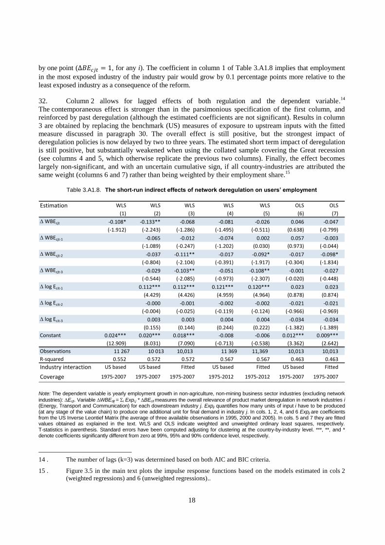
31. Table 3.A1.8 shows that, in the short-run, the impact of service deregulation on users’ employment

is uncertain as it varies depending on the estimation method and sample used. The baseline results in column

1 use US input-output coefficients as a measure of exposure, weights observations by their employment share

and considers only the contemporaneous impact of deregulation, imposing 𝜃𝑘 = 𝜌𝑘 = 0 for any k. The

estimated coefficient indicates that lowering anti-competitive regulation in network industries has a

significant and positive effect on users’ employment. One way to get a sense of the size of this effect is

thinking of two industries whose overall exposure to the regulated inputs (𝐸𝑥𝑝𝑗 = ∑ 𝐸𝑥𝑝𝑖,𝑗𝑗 ) differs by

one percentage point.13

Also, consider a policy that uniformly lowered regulation in the three industries

13 . Overall exposure (Expj) therefore measures output rises in Energy, Transportation and Communication

industries that is activated to by a unit increase in j’s final demand (i.e. the strength of j-induced backward

linkages in network industries).

18

by one point (∆𝐵𝐸𝑐𝑗𝑡 = 1, for any i). The coefficient in column 1 of Table 3.A1.8 implies that employment

in the most exposed industry of the industry pair would grow by 0.1 percentage points more relative to the

least exposed industry as a consequence of the reform.

32. Column 2 allows for lagged effects of both regulation and the dependent variable.14

The contemporaneous effect is stronger than in the parsimonious specification of the first column, and

reinforced by past deregulation (although the estimated coefficients are not significant). Results in column

3 are obtained by replacing the benchmark (US) measures of exposure to upstream inputs with the fitted

measure discussed in paragraph 30. The overall effect is still positive, but the strongest impact of

deregulation policies is now delayed by two to three years. The estimated short term impact of deregulation

is still positive, but substantially weakened when using the collated sample covering the Great recession

(see columns 4 and 5, which otherwise replicate the previous two columns). Finally, the effect becomes

largely non-significant, and with an uncertain cumulative sign, if all country-industries are attributed the

same weight (columns 6 and 7) rather than being weighted by their employment share.15

Table 3.A1.8. The short-run indirect effects of network deregulation on users’ employment

Note: The dependent variable is yearly employment growth in non-agriculture, non-mining business sector industries (excluding network

industries): DEcjt. Variable DWBEdjt = i Expi,j * DBEcit measures the overall relevance of product market deregulation in network industries i

(Energy, Transport and Communication) for each downstream industry j. Expji quantifies how many units of input i have to be produced (at any stage of the value chain) to produce one additional unit for final demand in industry j. In cols. 1, 2, 4, and 6 Expji are coefficients from the US Inverse Leontief Matrix (the average of three available observations in 1995, 2000 and 2005). In cols. 5 and 7 they are fitted values obtained as explained in the text. WLS and OLS indicate weighted and unweighted ordinary least squares, respectively. T-statistics in parenthesis. Standard errors have been computed adjusting for clustering at the country-by-industry level. ***, **, and * denote coefficients significantly different from zero at 99%, 95% and 90% confidence level, respectively.

14 . The number of lags (k=3) was determined based on both AIC and BIC criteria.

15 . Figure 3.5 in the main text plots the impulse response functions based on the models estimated in cols 2

(weighted regressions) and 6 (unweighted regressions)..

Estimation WLS WLS WLS WLS WLS OLS OLS

(1) (2) (3) (4) (5) (6) (7)

D WBEcjt -0.108* -0.133** -0.068 -0.081 -0.026 0.046 -0.047

(-1.912) (-2.243) (-1.286) (-1.495) (-0.511) (0.638) (-0.799)

D WBEcjt-1 -0.065 -0.012 -0.074 0.002 0.057 -0.003

(-1.089) (-0.247) (-1.202) (0.030) (0.973) (-0.044)

D WBEcjt-2 -0.037 -0.111** -0.017 -0.092* -0.017 -0.098*

(-0.804) (-2.104) (-0.391) (-1.917) (-0.304) (-1.834)

D WBEcjt-3 -0.029 -0.103** -0.051 -0.108** -0.001 -0.027

(-0.544) (-2.085) (-0.973) (-2.307) (-0.020) (-0.448)

D log Ecit-1 0.112*** 0.112*** 0.121*** 0.120*** 0.023 0.023

(4.429) (4.426) (4.959) (4.964) (0.878) (0.874)

D log Ecit-2 -0.000 -0.001 -0.002 -0.002 -0.021 -0.021

(-0.004) (-0.025) (-0.119) (-0.124) (-0.966) (-0.969)

D log Ecit-3 0.003 0.003 0.004 0.004 -0.034 -0.034

(0.155) (0.144) (0.244) (0.222) (-1.382) (-1.389)

Constant 0.024*** 0.020*** 0.018*** -0.008 -0.006 0.012*** 0.009***

(12.909) (8.031) (7.090) (-0.713) (-0.538) (3.362) (2.642)

Observations 11 267 10 013 10,013 11 369 11,369 10,013 10,013

R-squared 0.552 0.572 0.572 0.567 0.567 0.463 0.463

Industry interaction US based US based Fitted US based Fitted US based Fitted

Coverage 1975-2007 1975-2007 1975-2007 1975-2012 1975-2012 1975-2007 1975-2007

19

33. Exploring possible dimensions of heterogeneity did not help identify a subset of policies or

downstream industries for which deregulation has univocally negative (or positive) effects. Specifically,

the analysis i) looked at different dimensions of PMR reforms, comparing pro-competitive reforms to entry

with privatization (another dimension of regulation captured by the OECD indicators); ii) allowed for

reforms in each of the three upstream industries to have different relevance (i.e. different 𝜃𝑖,𝑘), and

iii) allowed the impact to vary between manufacturing and service users (as before, the presumption is that,

by operating in a more competitive environment the former might benefit more from enhanced upstream

competition).16

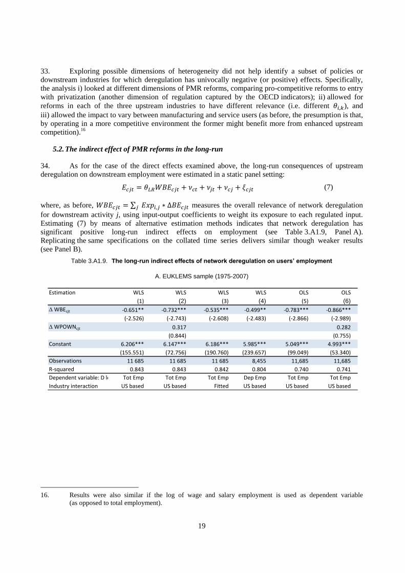
5.2. The indirect effect of PMR reforms in the long-run

34. As for the case of the direct effects examined above, the long-run consequences of upstream

deregulation on downstream employment were estimated in a static panel setting:

𝐸𝑐𝑗𝑡 = 𝜃𝐿𝑅𝑊𝐵𝐸𝑐𝑗𝑡 + 𝜈𝑐𝑡 + 𝜈𝑗𝑡 + 𝜈𝑐𝑗 + 𝜉𝑐𝑗𝑡 (7)

where, as before, 𝑊𝐵𝐸𝑐𝑗𝑡 = ∑ 𝐸𝑥𝑝𝑖,𝑗 ∗ ∆𝐵𝐸𝑐𝑗𝑡𝑗 measures the overall relevance of network deregulation

for downstream activity j, using input-output coefficients to weight its exposure to each regulated input.

Estimating (7) by means of alternative estimation methods indicates that network deregulation has

significant positive long-run indirect effects on employment (see Table 3.A1.9, Panel A).

Replicating the same specifications on the collated time series delivers similar though weaker results

(see Panel B).

Table 3.A1.9. The long-run indirect effects of network deregulation on users’ employment

A. EUKLEMS sample (1975-2007)

16. Results were also similar if the log of wage and salary employment is used as dependent variable

(as opposed to total employment).

Estimation WLS WLS WLS WLS OLS OLS

(1) (2) (3) (4) (5) (6)

D WBEcjt -0.651** -0.732*** -0.535*** -0.499** -0.783*** -0.866***

(-2.526) (-2.743) (-2.608) (-2.483) (-2.866) (-2.989)

D WPOWNcjt 0.317 0.282

(0.844) (0.755)

Constant 6.206*** 6.147*** 6.186*** 5.985*** 5.049*** 4.993***

(155.551) (72.756) (190.760) (239.657) (99.049) (53.340)

Observations 11 685 11 685 11 685 8,455 11,685 11,685

R-squared 0.843 0.843 0.842 0.804 0.740 0.741

Dependent variable: D log Employment. Variable WBEdjt = Si Expi,j * BEcit measures the overall stringency of product market regulation in network industries i (Energy, Transport and Communication) for each downstream industry j. Expji are coefficients froTot Emp Tot Emp Tot Emp Dep Emp Tot Emp Tot Emp

Industry interaction US based US based Fitted US based US based US based

20

Table 3.A1.9. The long-run indirect effects of network deregulation on users’ employment (cont.)

B. Collated EUKLEMS STAN sample (1975-2012)

Note: The dependent variable is the log of employment in non-agriculture, non-mining business sector industries (excluding network industries), except column 4 where it is measured in terms of salaried and wage employment. Estimates in Pane A use the Euklems (1975-2007) sample, while those in Panel B use a collated Euklems-STAN sample, extending the time coverage to 2012. This dataset is obtained mapping the OECD STAN industry classification (ISIC rev.4) to the 3-digit level using 3-digit level

employment data from EU LFS. Variable WBEdjt = i Expi,j * BEcit measures the overall relevance of product market regulation in

network industries i (Energy, Transport and Communication) for each downstream industry j. Expji quantifies how many units of input i have to be produced (at any stage of the value chain) to produce one additional unit for final demand in industry j. It is measured by

the coefficients from the US Inverse Leontief Matrix (the average of three available observations in 1995, 2000 and 2005), except in col. 3, where Expji is a fitted value obtained as explained in paragraph 30. WLS and OLS indicate weighted and unweighted ordinary least squares, respectively. T-statistics in parenthesis. Standard errors adjusted for clustering at the country-by-industry level. ***, **, and * denote coefficients significantly different from zero at 99%, 95% and 90% confidence level, respectively.

35. The baseline estimate in the first column of Panel A is obtained using the US based index of industry

dependence on the regulated service, exploiting the EUKLEMS data only (i.e. limiting the analysis to the 30 years

before the last financial crisis) and weighting observations in each country-industry share using employment shares

(i.e. attributing lower importance to smaller industries). One way to get a sense of its implications is to consider

two industries whose overall service dependence (𝐸𝑥𝑝𝑗 = ∑ 𝐸𝑥𝑝𝑖,𝑗𝑖 ) differ by one percentage point.17

Also, consider a policy that uniformly lowered regulation in the three service industries by one point.

The estimated coefficient in column 1 implies that long-run employment would be 0.65 percentage points higher

in the more exposed industry relative to the less exposed industry. For reference, overall service dependence

ranges from 4.7% (in Real Estate Activities) to 17.8% (in Other Non-Metallic Mineral Products).

36. This baseline result is robust to a large set of checks. In the second column of Panel A the specification

is augmented to account for the potentially confounding role of public ownership (the extent of state control in

network industries); column 3 replaces US input-output coefficients with the fitted indexes of industry exposure;

and column 4 changes the outcome variables using the growth rate of wage and salary (as opposed to total)

employment. Columns 5 and 6 show unweighted versions of the first two specifications. In all cases, the estimated

coefficient changes only slightly, both below and above the value estimated in the first column, and remains highly

statistically significant. The baseline result in column 1 is fairly stable to dropping one country at a time

(see Figure 3.A1.5).18

Importantly, the effect is also estimated to be stronger among manufacturing industries than

among services, confirming that greater upstream competition is particularly beneficial to firms in tradable

activities. Finally, the analysis also allowed the coefficient to vary with the level of regulation, exploring

17 . As in the case discussed in section 5.1, for each downstream industry j Expj measures the demand of

Energy, Transportation and Communication services that is activated to satisfy one additional unit of final

demand of the industry production.

18 . The estimated impact the overall relevance of network deregulation (𝑊𝐵𝐸) increases (respectively, falls)

the most dropping Japan (respectively, Korea). However, dropping both countries yields an estimate only

slightly below the baseline (0.55) and highly statistically significant.

Estimation WLS WLS WLS WLS OLS OLS

(1) (2) (3) (4) (5) (6)

D WBEcjt -0.347 -0.438* -0.266 -0.328* -0.411* -0.509**

(-1.450) (-1.721) (-1.438) (-1.689) (-1.735) (-1.991)

D WPOWNcjt 0.292 0.288

(0.993) (-1.859)

Constant 6.055*** 6.031*** 6.046*** 5.852*** 4.875*** 4.853***

(199.423) (147.897) (229.788) (251.715) -132.242 (-114.195)

Observations 13,041 13,041 13,041 9,848 13 041 13 041

R-squared 0.845 0.846 0.845 0.806 0.744 0.745

Dependent variable: D log Employment. Variable WBEdjt = Si Expi,j * BEcit measures the overall stringency of product market regulation in network industries i (Energy, Transport and Communication) for each downstream industry j. Expji are coefficients froTot Emp Tot Emp Tot Emp Dep Emp Tot Emp Tot Emp

Industry interaction US based US based Fitted US based US based US based

21

whether the strength of a given reform differs when this is taken in a high relatively to a low regulated

country. This was obtained augmenting the baseline specification (1) with the interaction between 𝑊𝐵𝐸𝑐𝑗𝑡

and a dummy variable 𝐻𝑅𝑒𝑔𝑐𝑡 indicating whether, in each country c, average regulation in the three

network industries was above or below the sample median. While the estimated 𝜃𝐿𝑅is unaffected, the

interaction term attracts a small coefficient which is not statistically significant. Hence, the data provide no

evidence that the impact of the reforms is non-linear on the level of regulation.

37. Panel B replicates the same set of regressions on the sample obtained collating EUKLEMS and

STAN industry data so to cover the Great Recession. As in the case of the short-run coefficients shown

in Table 3.A1.8, the size of the parameters estimated in this larger sample decreases (and the error around those

estimates becomes larger) relative to Panel A. These changes could reflect the lower strength of forward

linkages during the great recession induced, for example, by the slower entry of new firms in the reformed

upstream markets (see paragraph 2.3). But they could also simply reflect the measurement error introduced

when mapping the OECD STAN industry classification (ISIC rev.4) to the 3-digit level of EUKLEMS.

Figure 3.A1.5. The long-run indirect effects of network deregulation on users’ employment

Robustness to varying the country sample

Estimated impact the overall relevance of network deregulation (𝑊𝐵𝐸)

Note: The chart reports point estimates and 90%-confidence intervals of the long-run indirect effects of network deregulation of barriers to entry on users’ employment (specification (7)). Each dot indicates the coefficient estimated dropping from the sample the country indicated in the X-axis. The horizontal line represents the baseline coefficient estimated in col. 1 of Table 3.A1.9. Estimates refer to the case of a reform simultaneously lowering the OECD indicator of barriers to entry in each network industry (Energy, Transport and Communication, ETCR) by one point. The underlying parameters are estimated allowing employment growth in each network industry to depend on lagged values of industry regulation as well as on lagged employment changes. Confidence intervals are obtained by clustering errors on countries and industries.

Source: OECD estimates based on EUKLEMS and the OECD PMR Database.

38. The long-run indirect effects of network deregulation on industry wages (i.e. estimated using the log of

wages as dependent variable in specification (7)) are statistically insignificant. This holds irrespective of whether

the regressions conditions on employment and on the human capital composition of the employed or not.

39. How important would upstream reforms be for aggregate employment in downstream industries? In

principle, country-industry input-dependence models such as (7) only allow estimating the differential impact of

regulation on industry employment and do not lend themselves to infer the aggregate (i.e. country-level) impact of

lower regulation. The reason is that in the empirical specification cross-country variation – both in the dependent

and explanatory variables – is absorbed by country fixed effects. In practice, however, an answer to the above

-1.2

-1

-0.8

-0.6

-0.4

-0.2

0

JPN NLD FRA SWE POL FIN DEU ESP BEL CZE AUT GBR HUN PRT SVK ITA IRL DNK CAN AUS GRC KOR

All countries

22

question can be provided based on these models, conditional on a set of (strong) assumptions, discussed in Guiso

et al. (2004) and Bassanini et al. (2009). The main requirement is that one (or more) low-exposure industries

should be unaffected by the reform. The figures reported below are obtained under the (conservative) assumption

that, for any regulated service i, the reforms would have no effect in industries whose dependence on the regulated

service (𝐸𝑥𝑝𝑖𝑗) is lower than (or equal to) the first quartile of the distribution of dependence.

40. Given these assumptions, the aggregate effect of lowering entry barriers (∆𝐵𝐸𝑐𝑖) can be

computed adapting the two-step procedure devised by Guiso et al. (2004). In the first step, the estimated

coefficient θ is used to predict the employment gains in country c, industry j: ∆𝑙𝑛�̂�𝑐𝑗 = 𝜃𝐿𝑅 ∗

∑ 𝐸𝑥𝑝𝑖,𝑗 ∗ ∆𝐵𝐸𝑐𝑖𝑖 , In the second step, industry-specific gains are aggregated at the country level ∆𝑙𝑛�̂�𝑐 =

∑ 𝑆ℎ𝑗𝑐 ∗ ∆𝑙𝑛�̂�𝑐𝑗𝑗 , where 𝑆ℎ𝑗𝑐 is the (employment) share of industry j in country c.

41. This procedure was applied to the case of a hypothetical reform uniformly lowering regulation in

the three network industries by one point, in a prototypical country with the average industry employment

shares of the countries in the sample (this average was measured in the latest year for which all countries

are available). Long-run employment in downstream industries is estimated to increase by around 1%,

based on the baseline regression estimates shown in Panel A of Table 3.A1.9.19

42. Figure 3.4 in the main text provides an alternative representation plotting the estimated gains that

would be possible if OECD countries lowered regulation in each of the three service industries from their

latest observed level (around 2012) to the ‘‘lightest practice’’. Following Bourlès et al (2013), this is

defined as the average of the three lowest levels of anticompetitive regulation observed across countries.20

Based on the estimated coefficient in col. 1 (Panel A), the (simple) average gains across OECD countries

would be about 2%.

19 . The implied gains based on the weaker estimates from the collated sample (reported in Panel B) would be

of about 0.6%.

20 . More in detail, long-run employment would expand in excess of 3% in high regulated countries as Mexico,

Israel or Korea, and by less than 1% in countries that are already close to (or represent) the best practices

(as the United Kingdom or Australia).

23

References

Alesina, A., S. Ardagna, G. Nicoletti and F. Schiantarelli (2005), “Regulation and Investment,” Journal of

the European Economic Association, Vol. 3, No 4, pp. 791-825.

Bassanini, A. (2015), “A bitter medicine? Short-term employment impact of deregulation in network

industries”, IZA Discussion Paper No. 9187, Bonn.

Bassanini, A., L. Nunziata and D. Venn (2009), “Job Protection Legislation and Productivity Growth in

OECD Countries”, Economic Policy, Vol. 58, pp. 349-402.

Bourlès, R., Cette, G., Lopez, J., Mairesse, J. and Nicoletti, G. (2013), “Do Product Market Regulations In

Upstream Sectors Curb Productivity Growth? Panel Data Evidence for OECD Countries, ” The

Review of Economics and Statistics, Vol. 95, No.5, pp. 1750-1768.

Ciccone, A., and E. Papaioannou (2007), “Red Tape and Delayed Entry”, Journal of the European

Economic Association, Vol. 5, No. 2–3, pp. 444–458.

Guiso L., T. Jappelli, M. Padula and M. Pagano (2004) "Financial market integration and economic growth

in the EU," Economic Policy, Vol. 19, No. 40, pp. 523-577, October.

Nickell, S. (1981), “Biases in Dynamic Models with Fixed Effects”, Econometrica, Vol. 49, No. 6,

pp. 1417-1426.

Rajan, R. and L. Zingales (1998), “Financial Dependence and Growth”, American Economic Review,

Vol. 88, pp. 559-586.

Teulings, C. and N. Zubanov (2014), “Is Economic Recovery a Myth? Robust Estimation of Impulse

Responses”, Journal of Applied Econometrics, Vol. 29, pp. 497-514.

24

ANNEX 3.A2 REFORMS OF DISMISSAL LEGISLATION:

EMPIRICAL METHODOLOGY AND DETAILED ECONOMETRIC RESULTS

1. Introduction

43. This Annex presents the empirical methodologies adopted in the analysis of Chapter 3, Section 2.

It also reports the underlying estimates, robustness tests and extensions.

2. Cross-country/cross-industry/time-series analysis

2.1. Data and estimation methodology

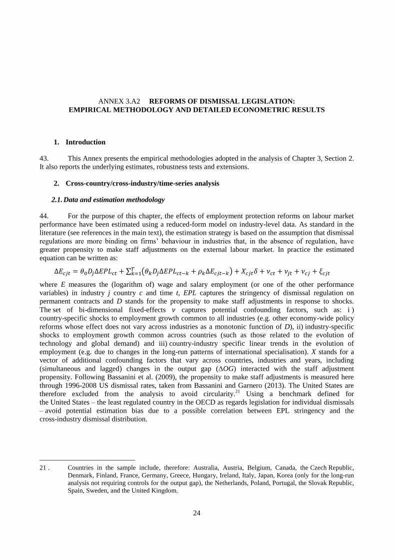
44. For the purpose of this chapter, the effects of employment protection reforms on labour market

performance have been estimated using a reduced-form model on industry-level data. As standard in the

literature (see references in the main text), the estimation strategy is based on the assumption that dismissal

regulations are more binding on firms’ behaviour in industries that, in the absence of regulation, have

greater propensity to make staff adjustments on the external labour market. In practice the estimated

equation can be written as:

∆𝐸𝑐𝑗𝑡 = 𝜃0𝐷𝑗∆𝐸𝑃𝐿𝑐𝑡 + ∑ (𝜃𝑘𝐷𝑗∆𝐸𝑃𝐿𝑐𝑡−𝑘 + 𝜌𝑘∆𝐸𝑐𝑗𝑡−𝑘)𝑇𝑘=1 + 𝑋𝑐𝑗𝑡𝛿 + 𝜈𝑐𝑡 + 𝜈𝑗𝑡 + 𝜈𝑐𝑗 + 𝜉𝑐𝑗𝑡

where E measures the (logarithm of) wage and salary employment (or one of the other performance

variables) in industry j country c and time t, EPL captures the stringency of dismissal regulation on

permanent contracts and D stands for the propensity to make staff adjustments in response to shocks.

The set of bi-dimensional fixed-effects 𝜈 captures potential confounding factors, such as: i )

country-specific shocks to employment growth common to all industries (e.g. other economy-wide policy

reforms whose effect does not vary across industries as a monotonic function of D), ii) industry-specific

shocks to employment growth common across countries (such as those related to the evolution of

technology and global demand) and iii) country-industry specific linear trends in the evolution of

employment (e.g. due to changes in the long-run patterns of international specialisation). X stands for a

vector of additional confounding factors that vary across countries, industries and years, including

(simultaneous and lagged) changes in the output gap (ΔOG) interacted with the staff adjustment

propensity. Following Bassanini et al. (2009), the propensity to make staff adjustments is measured here

through 1996-2008 US dismissal rates, taken from Bassanini and Garnero (2013). The United States are

therefore excluded from the analysis to avoid circularity.21

Using a benchmark defined for

the United States – the least regulated country in the OECD as regards legislation for individual dismissals

– avoid potential estimation bias due to a possible correlation between EPL stringency and the

cross-industry dismissal distribution.

21 . Countries in the sample include, therefore: Australia, Austria, Belgium, Canada, the Czech Republic,

Denmark, Finland, France, Germany, Greece, Hungary, Ireland, Italy, Japan, Korea (only for the long-run

analysis not requiring controls for the output gap), the Netherlands, Poland, Portugal, the Slovak Republic,

Spain, Sweden, and the United Kingdom.

25

45. Industry-level annual data used in the baseline sample are from EUKLEMS, which cover the

period 1975-2007 and allows recovering labour market outcomes for 22 industries in the

non-agricultural/non-mining business sector.22

The sample is extended to 2012 combining EUKLEMS with

the most recent version of OECD STAN.23

As regards the dependent variables, the analysis mainly

focusses on the logarithm of wage and salary employment.24

Other examined variables include the

logarithm of average hourly wages and the percentage share of those with less than upper secondary

education in hours worked. The output gap is taken from the OECD EO database.

46. The stringency of regulation is captured by the OECD indicator of EPL for regular contracts

(individual dismissals), which vary between 0 and 6 from the least to the most restrictive. Table 3.A3.2

reports the latest available data for OECD countries, comparing them with the regulation on temporary

forms of employment and the protection of permanent workers against individual and collective dismissals.

This indicator is available since 1985 at the earliest, which limits the EUKLEMS base sample to

1985-2007 and the extended EUKLEMS-STAN sample to 1985-2012. As the EPL indicators have

historically moved upwards and downwards, the analysis allows for heterogeneity between the effect of

flexibility-enhancing (indicator-reducing) and protection-raising (indicator increasing) reforms. In

addition, changes in the EPL indicators are typically small, rare and measured with significant error (see

OECD, 2013, and below). For this reason, in the baseline model, flexibility-enhancing EPL reforms are

measured through a dummy variable taking value 1 when the EPL indicator decreases and 0 otherwise. So

doing, the estimated coefficients capture the change in labour market performance associated with a reform

of historically average extensiveness (0.2 points), as measured by the average negative changes of the

indicator across all reform episodes of the sample. Similarly, protection-raising reforms are captured by a

dummy variable taking value 1 when the EPL indicator increases and 0 otherwise. Formally the estimation

model can be written as:

∆𝐸𝑐𝑗𝑡 = 𝜃0𝐷𝑗𝐹𝐸𝑐𝑡 + 𝜇0𝐷𝑗𝑃𝑅𝑐𝑡 + ∑ (𝜃𝑘𝐷𝑗𝐹𝐸𝑐𝑡−𝑘 + 𝜇𝑘𝐷𝑗𝑃𝑅𝑐𝑡−𝑘 + 𝜌𝑘∆𝐸𝑐𝑗𝑡−𝑘)𝑇𝑘=1 + 𝑋𝑐𝑗𝑡𝛿 + 𝕍 + 𝜉𝑐𝑗𝑡 (1)

where FE and PR stand for the flexibility-enhancing and protection-raising reform dummies, respectively,

and 𝕍 indicates the full set of double-dimensional fixed-effects. The optimal number of lags T is chosen on

the basis of Akaike’s and Bayesian information criteria, setting a maximum of T=3 for parsimony.

22 . The industry breakdown is an intermediate level between 1 and 2 digits of the ISIC rev. 3 classification and

approximately corresponds to the 2-letter level of the NACE rev.1 classification.

23 . OECD STAN is available for fewer but more recent years than EUKLEMS. The two dataset were collated

mapping the OECD STAN industry classification (ISIC rev.4) to the ISIC rev. 3 classification (used by

EUKLEMS). The mapping was obtained using 3-digit level employment data from EU LFS and tested on

years for which both classifications are available, but remains nonetheless imperfect. Accordingly, the

resulting sample is only used in sensitivity analysis (rather than as the preferred dataset). This is because

breaks in the industry classification can severely alter the estimated short-run dynamics and measurement

error induce bias in the estimated parameters. The same extension of the dataset cannot be replicated for

wages and the share of low-educated employees in hours worked.

24. In contrast with the PMR analysis, the analysis of EPL reforms investigates the effect on wage and salary

employment. In the PMR analysis, total employment was used instead, in order to exploit longer time

series of reliable data, with wage and salary employment being used only in sensitivity analyses. As in the

analysis of EPL reforms, the sample is anyhow limited to the post-1985 period by the availability of EPL

data (see below), wage and salary employment appears a more suitable dependent variable since the reform

effects are expected to be more important on dependent employment.

26

47. Quantitative indicators are used in an alternative model, which thus takes into account also the

extensiveness of the reforms. This model can be written as:

∆𝐸𝑐𝑗𝑡 = 𝜃0𝐷𝑗𝑆𝐹𝐸𝑐𝑡 + 𝜇0𝐷𝑗𝑆𝑃𝑐𝑡 + ∑(𝜃𝑘𝐷𝑗𝑆𝐹𝐸𝑐𝑡−𝑘 + 𝜇𝑘𝐷𝑗𝑆𝑆𝑃𝑐𝑡−𝑘 + 𝜌𝑘∆𝐸𝑐𝑗𝑡−𝑘)

𝑇

𝑘=1

+ 𝑋𝑐𝑗𝑡𝛿 + 𝕍 + 𝜉𝑐𝑗𝑡

where SFE and SP stand for the “size” of flexibility-enhancing and protection-raising reforms. SFE is

equal to the absolute change in the EPL indicator, when the latter is negative, and 0 otherwise. SP is equal

to the change in the EPL indicator, when the latter is positive, and 0 otherwise.

48. As discussed above, in equation (1) all omitted aggregate institutions are controlled for through

fixed effects. This is because their impact on the performance variable is unlikely to vary across industries

as a function of their dismissal intensity. As standard in this literature, the validity of this statement is

checked by including one-by-one interactions between the industry-specific US dismissal rate and other

observable labour market reforms, which turn out always insignificant as expected (see the next

subsection). Reverse causality is also less of a concern in this framework since it would imply that

economy-wide reforms are significantly affected by idiosyncratic fluctuations of specific industries, which

seems unlikely (indeed Bassanini et al., 2009, provide evidence that this is not the case). The sign of the

estimated parameters can therefore be given a causal interpretation.25

49. Impulse-response functions presented below and in the main text are derived using the local

projection estimator developed by Teulings and Zubanov (2014), which is a variant of that of Jordà (2005).

The algorithm allows estimating the cumulative response of the reform implemented at time t after 𝜏

periods (𝐶𝑅(𝜏)) by estimating a system of 𝜏 simultaneous equations:

∆𝐸𝑐𝑗𝑡+ℎ = ∑ 𝜃𝑓ℎ𝐷𝑗𝐹𝐸𝑐𝑡+𝑓ℎ𝑓=1 + ∑ 𝜃𝑘ℎ𝐷𝑗𝐹𝐸𝑐𝑡−𝑘

𝑇𝑘=0 + ∑ 𝜌𝑘ℎ∆𝐸𝑐𝑗𝑡−𝑘

𝑇𝑘=1 + 𝑋𝑐𝑗𝑡𝛿 + 𝕍 + 𝜉𝑐𝑗𝑡 (2)

for ℎ ∈ (0, 𝜏) and with X including PR and ΔOG interacted with D and with the same number of lags and

forwards as FE.26

T is optimally chosen for h=0 and is therefore the same as for equation (1).

The cumulative impact of the reform is defined as the sum of the coefficients estimated on the variable FE

in each equation: 𝐶𝑅(𝜏) = ∑ 𝜃0ℎ𝜏ℎ=0 .

27 The variables in the first term on the right-hand side

(∑ 𝜃𝑓ℎ𝐷𝑗𝐹𝐸𝑐𝑡+𝑓ℎ𝑓=1 ), as well as the corresponding forward terms of PR and ΔOG are introduced to capture

the potentially confounding effects of reforms and shocks occurring after time t. The minimum value of 𝜏

for which 𝐶𝑅(𝜏) is not significantly different from 0 will indicate the duration of the employment impact

of reforms.

50. This setting allows several extensions of the empirical specification. One consists in testing for

potential heterogeneity in the effects of deregulation over the business cycle, which has potential

implications for the optimal timing of this type of structural reform. To this purpose, the dummy for

flexibility-enhancing reforms FE is interacted both with the industry US dismissal rate and the change in

the output gap (ΔOG). 28

As the output gap is defined as the difference between current and potential

25 . Strictly speaking, however, they represent the relative effect of flexibility-enhancing EPL reforms between

two industries that are 1 percentage point apart in terms of dismissal rates.

26 . In contrast with the PMR analysis (see e.g. Box 3.1 in the main text), impulse responses are computed also

accounting for the contemporaneous coefficient (𝜃00), as reverse causality issues are not a concern in this

framework.

27. Note that, except for the first term, the right hand side of this specification is the same as in equation (1).

28 . Replicating the same analysis using OG yields estimates of the interaction terms that are insignificantly

different from 0.

27

output, ΔOG takes negative values when the economy is in a downturn. Hence, a positive sign on this

interaction would suggest that the short-run employment costs from deregulation are aggravated by

worsening economic conditions and attenuated in upswings. In the same way one can also test whether the

effect of EPL liberalisation is stronger or weaker in different institutional frameworks, as measured by the

level of another aggregate variable. However, caution must be exerted in interpreting interactions between

aggregate structural variables (which usually yield estimates whose magnitude and sign are not robust to

changes in the specification; see e.g. Bassanini and Duval, 2009, for a discussion). For this reason, in this

analysis, the only interaction of this type that is considered is that between D*FE and the share of

fixed-term contracts in wage-and-salary employment, taken from the OECD Employment Database.

The reason is that, for a limited number of years and countries, this variable is also available at the

industry-level (source Bassanini and Garnero, 2013), which allows a sharper identification (even though

estimated coefficients are less clearly interpretable). Estimates obtained using the industry-level variables

confirm those presented below that are obtained using the aggregate variable and a larger sample.

51. Rigorously speaking, the approach adopted here allows identifying only differential effects

between EPL-binding and other industries. However, as the effect of EPL on firms’ staff adjustment

policies (the direct effect of EPL) depends on the extent to which regulations are binding, it is unlikely that

dismissal regulations have opposite effects on these policies in binding and non-binding industries.

Under the reasonable assumption that the sign of the direct effect of EPL reforms is not opposite in

industries where regulation is binding and in those where it is not, the sign of the estimated s can be used

for making inference on the sign of the overall aggregate effect of EPL reforms if general equilibrium

effects do not offset the direct impact. As regards general equilibrium effects, it has been argued that

greater separations in EPL-binding industries in the aftermath of flexibility-enhancing reforms could

increase labour supply and employment in other industries (Zweimüller, 2009). Yet, Bassanini

and Garnero (2013), using multiple identification strategies, find no long-run effect of EPL for regular

contracts on either job-to-jobless separations or job-to-job ones entailing a change of industry. Moreover,

for this chapter, the analysis of equation (1) was replicated using Bassanini and Garnero’s data on

separations and T=0.29

The results suggest that 73% of the increase in separations in the aftermath of

flexibility-enhancing EPL reforms is due to job-to-job separations within the same industry, while only 6%

is due to transitions involving an industry change. 30

This suggests that general equilibrium effects of this

type are minor in this context and that the sign of the estimated s provides also an indication of the sign of

the aggregate effect of EPL reforms, as in standard difference-in-difference models. Yet, insofar as there

might be other second-order general-equilibrium mechanisms at play, offsetting the direct impact of

EPL reforms, the next section compares the signs of the aggregate effects on employment computed in this

one with those on unemployment estimated using a regression-discontinuity approach on high-frequency

aggregate data. If offsetting general equilibrium mechanisms were relevant, the two exercises should lead

to very different conclusions on the labour market consequences of EPL reforms. This does not turn out to

be the case.

52. A cautious quantitative assessment of these aggregate effects can then be derived taking into

account the relative size of business-sector industries and imposing the conservative assumption that

EPL reforms would have no short-term effect on employment in industries where dismissal regulations are

not binding, defining the latter as those whose US dismissal rate would be equal to or lower than the first

quartile of the distribution.

29 . T is set equal to 0 for parsimony since data on separations are available only for

a short-time window (1995-2007).

30 . Transitions are defined over an one-year horizon.

28

53. Following Bassanini et al. (2009) and OECD (2012), the long-term effects of EPL are estimated

by adapting the above model to a simple static framework. This can be written as:

𝐸𝑐𝑗𝑡 = 𝜃𝐿𝑅𝐷𝑗𝐸𝑃𝐿𝑐𝑡 + 𝑋𝑐𝑗𝑡𝛿𝐿𝑅 + 𝜈𝑐𝑡 + 𝜈𝑗𝑡 + 𝜈𝑐𝑗 + 𝜉𝑐𝑗𝑡. (3)

where the LR suffix indicates long-run parameters. To the extent that, as discussed above, long-run

cross-industry general equilibrium effects appear minor, the aggregate long-run effect of EPL for regular

contracts on labour market performance in the business-sector can be derived using the same methodology

as for short-run effects.

2.2. Results

54. Table 3.A2.1 reports estimates obtained with weighted and unweighted regressions in Panels A

and B, respectively. Column 1 of Panel A reports estimated coefficients from the baseline specification

(used for Figure 3.5 in the main text).31

From a quantitative point of view it suggests that, comparing two

industries that are 1 percentage point apart in terms of dismissal rates – corresponding to about 60% of a

standard deviation of the cross-industry distribution of US dismissal rates, the contraction of wage and

salary employment in the year following an average EPL reform is estimated to be larger by 0.29% in the

most dismissal-intensive industry. The comparison of coefficients among the first four columns of both

panels indicates that coefficient estimates are robust to the selection of the number of lags, choice of the

sample (base or extended) and use of either weighted OLS or simple OLS.32

However, the recovery from

the initial negative effect is estimated to be somewhat faster in the case of unweighted regressions, as

shown by the corresponding impulse-response functions (Figure 3.A2.1).33

31. Strictly speaking, column 1 of Panel A presents only the model used to compute the value at lag 0 of

Figure 3.5. By contrast, the other values are obtained through the corresponding model with, still, 3 lags

but the required number of forwards (see equation (2) above).

32 . The same can be said for the case in which the share of the low-educated is used as dependent variable. In

the case of wages, the estimated effect appears somewhat sensitive to the use of weights.

33. Panel A reports the same function as shown in Figure 3.5 to facilitate the comparison.

29

Table 3.A2.1. Baseline estimates: EPL reforms

Notes: Dependent variables are changes in log wage and salary employment, log average wage or percentage share of those with less than upper secondary education in hours worked, as indicated in column titles. FE: dummy variable for flexibility-enhancing reforms of EPL for regular contracts; DR: industry-level US dismissal rate (in %). All specifications control for lags of changes in log employment (same number as for FE*DR), changes in the output gap and a dummy for protection-raising EPL reforms (both interacted with DR and also including the same number of lags as for FE*DR) as well as country-by-time, industry-by-time and country-by-industry dummies. The specification of Column 6 also controls for the change in the logarithm of wage and salary employment and of the share of low-educated employees in hours worked. The observations in Panel A are weighted by the average industry share in the country’s non-agricultural/non-mining business sector. The base sample is the EUKLEMS sample (1985-2007); the extended sample is the combined EUKLEMS-STAN sample (1985-2012). T-statistics, adjusted for clustering at the country-by-industry level, in parentheses. ***, **, and * denote coefficients significantly different from zero at 99%, 95% and 90% confidence level, respectively.

Base sample

Employment

Base sample

Employment

Extended

sample

Employment

Extended

sample

Employment

Base sample

Wage

Base sample

Wage

Base sample

Low-educated

share

(1) (2) (3) (4) (5) (6) (7)

FEt*DR -0.0029* -0.0030* -0.0031** -0.0033** -0.0005 -0.0014 0.0004

(-1.77) (-1.79) (-2.14) (-2.15) (-0.32) (-1.14) (0.01)

FE t-1*DR -0.0009 -0.0009 -0.0004 -0.0006 -0.0023* -0.0022* 0.0466

(-0.57) (-0.65) (-0.24) (-0.42) (-1.96) (-1.84) (1.26)

FE t-2*DR 0.0009 0.0008 0.0003 0.0003 -0.0003 0.0000 0.0324

(0.57) (0.58) (0.23) (0.21) (-0.24) (0.03) (0.78)

FE t-3*DR 0.0001 0.0005 0.0013 0.0002 -0.0085

(0.07) (0.28) (0.80) (0.10) (-0.17)

Observations 7,590 8,052 9,091 9,574 7,590 6,622 6,424

R-squared 0.532 0.510 0.529 0.524 0.369 0.434 0.552

Base sample

Employment

Base sample

Employment

Extended

sample

Employment

Extended

sample

Employment

Base sample

Wage

Base sample

Wage

Base sample

Low-educated

share

(1) (2) (3) (4) (5) (6) (7)

FEt*DR -0.0032** -0.0033* -0.0027* -0.0027* 0.0007 -0.0001 0.0046

(-1.98) (-1.93) (-1.89) (-1.78) (0.53) (-0.09) (0.13)

FE t-1*DR 0.0018 0.0020 0.0021 0.0021 -0.0023* -0.0010 0.0152

(0.89) (1.01) (1.03) (1.10) (-1.75) (-0.94) (0.46)

FE t-2*DR 0.0012 0.0014 0.0007 0.0007 -0.0021 0.0003 -0.0486

(0.85) (1.09) (0.58) (0.67) (-1.34) (0.27) (-1.23)

FE t-3*DR -0.0007 -0.0010 0.0002 -0.0004 -0.0592

(-0.45) (-0.47) (0.14) (-0.32) (-1.40)

Observations 7,590 8,052 9,091 9,574 7,590 6,622 6,424

R-squared 0.399 0.390 0.400 0.394 0.290 0.360 0.538

A. Weighted regressions

B. Unweighted regressions

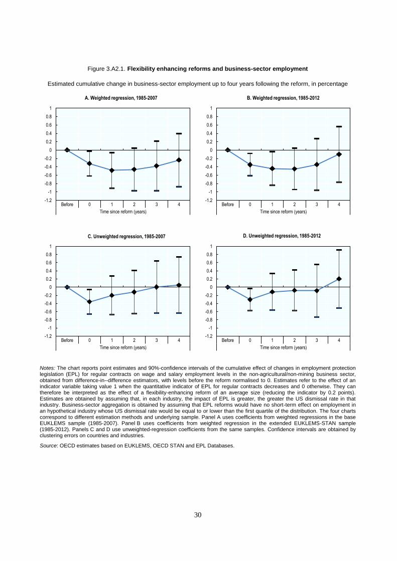
30

Figure 3.A2.1. Flexibility enhancing reforms and business-sector employment

Estimated cumulative change in business-sector employment up to four years following the reform, in percentage

Notes: The chart reports point estimates and 90%-confidence intervals of the cumulative effect of changes in employment protection legislation (EPL) for regular contracts on wage and salary employment levels in the non-agricultural/non-mining business sector, obtained from difference-in--difference estimators, with levels before the reform normalised to 0. Estimates refer to the effect of an indicator variable taking value 1 when the quantitative indicator of EPL for regular contracts decreases and 0 otherwise. They can therefore be interpreted as the effect of a flexibility-enhancing reform of an average size (reducing the indicator by 0.2 points). Estimates are obtained by assuming that, in each industry, the impact of EPL is greater, the greater the US dismissal rate in that industry. Business-sector aggregation is obtained by assuming that EPL reforms would have no short-term effect on employment in an hypothetical industry whose US dismissal rate would be equal to or lower than the first quartile of the distribution. The four charts correspond to different estimation methods and underlying sample. Panel A uses coefficients from weighted regressions in the base EUKLEMS sample (1985-2007). Panel B uses coefficients from weighted regression in the extended EUKLEMS-STAN sample (1985-2012). Panels C and D use unweighted-regression coefficients from the same samples. Confidence intervals are obtained by clustering errors on countries and industries.

Source: OECD estimates based on EUKLEMS, OECD STAN and EPL Databases.

-1.2

-1

-0.8

-0.6

-0.4

-0.2

0

0.2

0.4

0.6

0.8

1

Before 0 1 2 3 4

Time since reform (years)

A. Weighted regression, 1985-2007

-1.2

-1

-0.8

-0.6

-0.4

-0.2

0

0.2

0.4

0.6

0.8

1

Before 0 1 2 3 4

Time since reform (years)

B. Weighted regression, 1985-2012

-1.2

-1

-0.8

-0.6

-0.4

-0.2

0

0.2

0.4

0.6

0.8

1

Before 0 1 2 3 4

Time since reform (years)

C. Unweighted regression, 1985-2007

-1.2

-1

-0.8

-0.6

-0.4

-0.2

0

0.2

0.4

0.6

0.8

1

Before 0 1 2 3 4

Time since reform (years)

D. Unweighted regression, 1985-2012

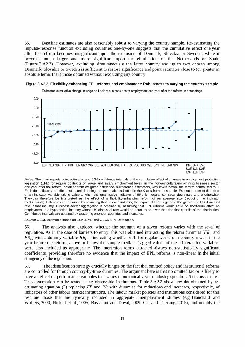
31

55. Baseline estimates are also reasonably robust to varying the country sample. Re-estimating the

impulse-response function excluding countries one-by-one suggests that the cumulative effect one year

after the reform becomes insignificant upon the exclusion of Denmark, Slovakia or Sweden, while it

becomes much larger and more significant upon the elimination of the Netherlands or Spain

(Figure 3.A2.2). However, excluding simultaneously the latter country and up to two chosen among

Denmark, Slovakia or Sweden is sufficient to restore significance and point estimates close to (or greater in

absolute terms than) those obtained without excluding any country.

Figure 3.A2.2. Flexibility-enhancing EPL reforms and employment: Robustness to varying the country sample

Estimated cumulative change in wage-and salary business-sector employment one year after the reform, in percentage

Notes: The chart reports point estimates and 90%-confidence intervals of the cumulative effect of changes in employment protection legislation (EPL) for regular contracts on wage and salary employment levels in the non-agricultural/non-mining business sector one year after the reform, obtained from weighted difference-in-difference estimators, with levels before the reform normalised to 0. Each dot indicates the effect estimated dropping the country/ies indicated in the X-axis from the sample. Estimates refer to the effect of an indicator variable taking value 1 when the quantitative indicator of EPL for regular contracts decreases and 0 otherwise. They can therefore be interpreted as the effect of a flexibility-enhancing reform of an average size (reducing the indicator by 0.2 points). Estimates are obtained by assuming that, in each industry, the impact of EPL is greater, the greater the US dismissal rate in that industry. Business-sector aggregation is obtained by assuming that EPL reforms would have no short-term effect on employment in a hypothetical industry whose US dismissal rate would be equal to or lower than the first quartile of the distribution. Confidence intervals are obtained by clustering errors on countries and industries.

Source: OECD estimates based on EUKLEMS and OECD EPL Databases.

56. The analysis also explored whether the strength of a given reform varies with the level of

regulation. As in the case of barriers to entry, this was obtained interacting the reform dummies (𝐹𝐸𝑡 and

𝑃𝑅𝑡) with a dummy variable 𝐻𝐸𝑡−1 indicating whether EPL for regular workers in country c was, in the

year before the reform, above or below the sample median. Lagged values of these interaction variables

were also included as appropriate. The interaction terms attracted always non-statistically significant

coefficients, providing therefore no evidence that the impact of EPL reforms is non-linear in the initial

stringency of the regulation.

57. The identification strategy crucially hinges on the fact that omitted policy and institutional reforms

are controlled for through country-by-time dummies. The argument here is that no omitted factor is likely to

have an effect on performance variables that varies monotonically with industry-specific US dismissal rates.

This assumption can be tested using observable institutions. Table 3.A2.2 shows results obtained by re-

estimating equation (2) replacing FE and PR with dummies for reductions and increases, respectively, of

indicators of other labour market institutions. The labour market policies and institutions considered for this

test are those that are typically included in aggregate unemployment studies (e.g. Blanchard and

Wolfers, 2000, Nickell et al., 2005, Bassanini and Duval, 2009, Gal and Theising, 2015), and notably the

-,1.20

-,1.00

-,0.80

-,0.60

-,0.40

-,0.20

,0.00

,0.20

ESP NLD GBR FIN PRT HUN GRC CAN BEL AUT DEU SWE ITA FRA POL AUS CZE JPN IRL DNK SVK DNKSWEESP

DNKSVKESP

SVKSWEESP

All countries

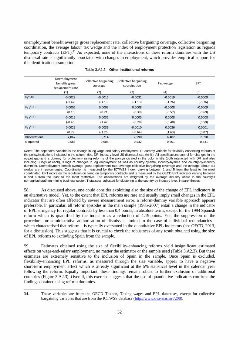
32

unemployment benefit average gross replacement rate, collective bargaining coverage, collective bargaining

coordination, the average labour tax wedge and the index of employment protection legislation as regards

temporary contracts (EPT).34

As expected, none of the interactions of these reform dummies with the US

dismissal rate is significantly associated with changes in employment, which provides empirical support for

the identification assumption.

Table 3.A2.2. Other institutional reforms

Notes: The dependent variable is the change in log wage and salary employment. R: dummy variable for flexibility-enhancing reforms of the policy/institutions indicated in the column title; DR: industry-level US dismissal rate (in %). All specifications control for changes in the output gap and a dummy for protection-raising reforms of the policy/indicated in the column title (both interacted with DR and also including 3 lags of each), 3 lags of changes in log employment as well as country-by-time, industry-by-time and country-by-industry dummies. Unemployment benefit average gross replacement rate, average collective bargaining coverage and the average labour tax wedge are in percentages. Coordination is measured by the ICTWSS index, varying between 1 and 5 from the least to the most coordinated. EPT indicates the regulation on hiring on temporary contracts and is measured by the OECD EPT indicator varying between 0 and 6 from the least to the most restrictive. The observations are weighted by the average industry share in the country’s non-agricultural/non-mining business sector. T-statistics, adjusted for clustering at the country-by-industry level, in parentheses.

58. As discussed above, one could consider exploiting also the size of the change of EPL indicators in

an alternative model. Yet, to the extent that EPL reforms are rare and usually imply small changes in the EPL

indicator that are often affected by severe measurement error, a reform-dummy variable approach appears

preferable. In particular, all reform episodes in the main sample (1985-2007) entail a change in the indicator

of EPL stringency for regular contracts by less than 0.4 points, in absolute terms, except for the 1994 Spanish

reform which is quantified by the indicator as a reduction of 1.19 points. Yet, the suppression of the

procedure for administrative authorisation of dismissals limited to the case of individual redundancies –

which characterised that reform – is typically overstated in the quantitative EPL indicators (see OECD, 2013,

for a discussion). This suggests that it is crucial to check the robustness of any result obtained using the size

of EPL reforms to excluding Spain from the sample.

59. Estimates obtained using the size of flexibility-enhancing reforms yield insignificant estimated

effects on wage-and-salary employment, no matter the estimator or the sample used (Table 3.A2.3). But these

estimates are extremely sensitive to the inclusion of Spain in the sample. Once Spain is excluded,

flexibility-enhancing EPL reforms, as measured through the size variable, appear to have a negative

short-term employment effect which is already significant at the 5% statistical level in the calendar year

following the reform. Equally important, these findings remain robust to further exclusion of additional

countries (Figure 3.A2.3). Overall, this exercise suggests that the use of quantitative indicators confirms the

findings obtained using reform dummies.

34. These variables are from the OECD Taxben, Taxing wages and EPL databases, except for collective

bargaining variables that are from the ICTWSS database (http://www.uva-aias.net/208).

Unemployment

benefits gross

replacement rate

Collective bargaining

coverage

Collective bargaining

coordinationTax wedge EPT

(1) (2) (3) (4) (5)

R t*DR -0.0029 -0.0015 -0.0031 -0.0019 -0.0009

(-1.42) (-1.13) (-1.13) (-1.26) (-0.76)

R t-1*DR 0.0005 0.0003 0.0008 -0.0008 -0.0009

(0.15) (0.21) (0.39) (-0.57) (-0.69)

R t-2*DR -0.0015 0.0035 0.0005 0.0008 0.0008

(-0.46) (1.47) (0.28) (0.48) (0.59)

R t-3*DR 0.0025 -0.0036 -0.0010 0.0026 0.0001

(0.78) (-1.26) (-0.64) (1.63) (0.07)

Observations 7,062 5,214 7,590 6,402 7,590

R-squared 0.583 0.604 0.532 0.601 0.531

33

Table 3.A2.3. Quantitative EPL indicators

Notes: The dependent variable is the change in log wage and salary employment. SFE: size of flexibility-enhancing EPL reforms measured as absolute change in EPL for regular contracts if negative and 0 otherwise; DR: industry-level US dismissal rate (in %). All specifications control for changes in the output gap and size of protection-raising EPL reforms (both interacted with DR and also including 3 lags of each), 3 lags of changes in log employment as well as country-by-time, industry-by-time and country-by-industry dummies. Columns 4 to 6 exclude observations from Spain. The observations are weighted by the average industry share in the country’s non-agricultural/non-mining business sector, except in columns 2 and 5. The base sample is the EUKLEMS sample (1985-2007); the extended sample is the combined EUKLEMS-STAN sample (1985-2012). T-statistics, adjusted for clustering at the country-by-industry level, in parentheses. ***, **, and * denote coefficients significantly different from zero at 99%, 95% and 90% confidence level, respectively.

Figure 3.A2.3. Quantitative indicators of flexibility-enhancing EPL reforms and employment: Robustness to varying the country sample

Estimated change in wage-and salary business-sector in the year following the reform, in percentage

Notes: The chart reports point estimates and 90%-confidence intervals of the effect of changes in employment protection legislation (EPL) for regular contracts on average year-on-year change in wage and salary employment levels in the non-agricultural/non-mining business sector in the calendar year following the reform, obtained from weighted difference-in-difference estimators. Each dot indicates the effect estimated dropping Spain and the country indicated in the X-axis from the sample. Estimates refer to the effect of a decrease of 1 point in the quantitative indicator of EPL for regular contracts (individual dismissals). Estimates are obtained by assuming that, in each industry, the impact of EPL is greater, the greater the US dismissal rate in that industry. Business-sector aggregation is obtained by assuming that EPL reforms would have no short-term effect on employment in a hypothetical industry whose US dismissal rate would be equal to or lower than the first quartile of the distribution. Confidence intervals are obtained by clustering errors on countries and industries.

Source: OECD estimates based on EUKLEMS and OECD EPL Databases.

Base sample,

all countries

Base sample,

all countries

Extended sample,

all countries

Base sample,

no Spain

Base sample,

no Spain

Extended sample,

no Spain

SFE t*DR 0.0027 -0.0079 -0.0019 -0.0206*** -0.0180** -0.0244***(-0.47) (-0.95) (-0.25) (-2.92) (-2.10) (-3.49)

SFE t-1*DR 0.0009 0.0102* 0.0035 -0.0054 0.0109 -0.0037(-0.20) (-1.87) (-0.85) (-0.50) (0.85) (-0.41)

SFE t-2*DR -0.0003 0.0009 0.0019 -0.0036 0.0060 -0.0041(-0.08) (-0.17) (-0.48) (-0.34) (0.71) (-0.41)

SFE t-3*DR 0.0034 0.0027 0.0060** 0.0050 0.0047 0.0062

(-1.47) (-0.77) (-1.97) (0.63) (0.65) (0.56)

Observations 7,590 7,590 9,091 7,172 7,172 8,629

R-squared 0.53 0.40 0.53 0.52 0.39 0.52

-5

-4.5

-4

-3.5

-3

-2.5

-2

-1.5

-1

-0.5

0

AUT FIN NLD IRL GBR CAN ESP BEL DNK FRA GRC SWE POL HUN DEU JPN ITA AUS CZE SVK PRT

All countries

34

60. Next, interactions with the business cycle are examined. Table 3.A2.4, shows the result of this

exercise for the main and extended samples. In the case of employment, the coefficients of the interaction

terms, if estimated on the base sample, are all positive and significant at lag 2. 35

However, this result is not

robust to the choice of the sample. This might be either due to the fact that the effect is non-linear in the

size of the change of the output gap (so that output-gap contractions larger than a certain threshold do not

increase further the post-reform employment drop) or might be the result of the imperfect matching of

EUKLEMS and STAN.

Table 3.A2.4. EPL reforms in upturns and downturns

Notes: Dependent variables are changes in log wage and salary employment, log average wage or percentage share of those with less than upper secondary education in hours worked, as indicated in column titles. FE: dummy variable for flexibility-enhancing reforms of EPL for regular contracts; DR: industry-level US dismissal rate (in %); OG: output gap (in %). All specifications control for lags of changes in log employment (same number as for FE*DR), changes in the output gap and a dummy for protection-raising EPL reforms (both interacted with DR and also including the same number of lags as for FE*DR) as well as country-by-time, industry-by-time and country-by-industry dummies. The observations are weighted by the average industry share in the country’s non-agricultural/non-mining business sector. The base sample is the EUKLEMS sample (1985-2007); the extended sample is the combined EUKLEMS-STAN sample (1985-2012). T-statistics, adjusted for clustering at the country-by-industry level, in parentheses. ***, **, and * denote coefficients significantly different from zero at 99%, 95% and 90% confidence level, respectively.

61. Interactions with the share of fixed-term contracts appear more robust to the choice of the sample

(Table 3.A2.5). Not only do all interaction terms are positive in the case of employment, but they are also

significant at the 5% statistical level at lag 0. A similar result is found in the case of the share of

the low-educated in hours worked. In the latter case, even though each coefficient is insignificant, their

sum is significant at lags 2 and 3, which explains the differences across panels in Figure 3.10 in the main

text. In the case of wages, no noteworthy interaction pattern emerges.

35. The short-term effects of reducing firing costs on wages or the low-educated share do not seem particularly

sensitive to business-cycle conditions.

Base sample,

Employment

Extended sample,

Employment

Base sample,

Wage

Base sample,

Low-educated share

FEt*DR -0.0030* -0.0029* -0.0006 -0.0022

(-1.77) (-1.95) (-0.33) (-0.05)

FE t-1*DR -0.0010 -0.0005 -0.0023* 0.0488

(-0.60) (-0.28) (-1.85) (1.43)

FE t-2*DR 0.0019 0.0006 -0.0001 0.0311

(1.48) (0.43) (-0.10) (0.77)

FE t-3*DR 0.0002 0.0004 0.0012 -0.0073

(0.15) (0.23) (0.81) (-0.15)

DOGt *FEt*DR 0.0101 0.0064 -0.0035 0.0785

(1.10) (0.76) (-0.31) (0.37)

DOG t-1*FE t-1*DR 0.0008 -0.0011 -0.0005 0.1130

(0.07) (-0.17) (-0.06) (0.45)

DOG t-2*FE t-2*DR 0.0227* 0.0102 0.0039 0.0100

(1.82) (1.04) (0.62) (0.03)

DOG t-3*FE t-3*DR 0.0018 -0.0008 -0.0038 0.2390

(0.18) (-0.11) (-0.36) (1.13)

Observations 7,590 9,091 7,590 6,424

R-squared 0.532 0.529 0.369 0.552

35

Table 3.A2.5. EPL reforms and the share of fixed-term contracts

Notes: Dependent variables are changes in log wage and salary employment, log average wage or percentage share of those with less than upper secondary education in hours worked, as indicated in column titles. FE: dummy variable for flexibility-enhancing reforms of EPL for regular contracts; DR: industry-level US dismissal rate (in %); ShT: Share of fixed-term contracts in wage and salary employment (in %). All specifications control for lags of changes in log employment (same number as for FE*DR), changes in the output gap, changes in the share of fixed-term contracts and a dummy for protection-raising EPL reforms (all three variables interacted with DR and also including the same number of lags as for FE*DR) as well as country-by-time, industry-by-time and country-by-industry dummies. The observations are weighted by the average industry share in the country’s non-agricultural/non-mining business sector. The base sample is the EUKLEMS sample (1985-2007); the extended sample is the combined EUKLEMS-STAN sample (1985-2012). T-statistics, adjusted for clustering at the country-by-industry level, in parentheses. ***, **, and * denote coefficients significantly different from zero at 99%, 95% and 90% confidence level, respectively.

62. Long-run effects of EPL are investigated in Table 3.A2.6. Consistent with the literature,

EPL does not appear to have a significant impact on wage-and-salary employment, no matter the dataset or

the estimator used (Columns 1 and 2 in both panels). Yet, this result is somewhat sensitive to the presence

of Korea in the sample.36

Once Korea is excluded from the base sample and the weighted estimator is used,

the degree of stringency of EPL for regular contracts is found to have a negative impact on employment –

that would imply a positive effect of EPL reforms– which is significant at the 10% statistical level

(Figure 3.A2.4, Panel A). But in the case of all other specifications in the table (Column 2 of Panel A and

Columns 1 and 2 of Panel B), the estimated coefficients of EPL remain insignificant upon exclusion of any

country in the dataset,37

which suggests that, overall, the evidence is consistent with the prediction of

no long-run effect of EPL on employment.

36. As equation (3) does not require the inclusion of the output gap as a covariate, Korea can be included in the

sample.

37 . Not shown in the Figure.

Base sample

Employment

Extended sample

Employment

Base sample

Wage

Base sample

Low-educated share

FEt*DR -0.0031 -0.0039** 0.0001 0.0795

(-1.63) (-2.24) (0.09) (1.38)

FE t-1*DR -0.0004 -0.0001 -0.0030** 0.0919**

(-0.20) (-0.08) (-1.98) (2.02)

FE t-2*DR 0.0019 0.0002 0.0001 0.1103*

(1.49) (0.12) (0.10) (1.81)

FE t-3*DR 0.0001 0.0004 0.0015 0.0305

(0.10) (0.23) (0.78) (0.48)

ShTt *FEt*DR 0.0056** 0.0057** -0.0027 -0.0089

(2.34) (2.21) (-1.54) (-0.15)

ShTt-1*FE t-1*DR 0.0031 0.0030 0.0010 0.0696

(1.15) (1.44) (0.68) (1.32)

ShTt-2*FE t-2*DR 0.0004 0.0023 -0.0011 0.0789

(0.26) (1.19) (-0.89) (1.31)

ShTt-3*FE t-3*DR 0.0017 -0.0000 -0.0021 0.0652

(1.24) (0.00) (-1.35) (0.67)

Observations 6,226 7,727 6,226 5,060

R-squared 0.506 0.511 0.373 0.583

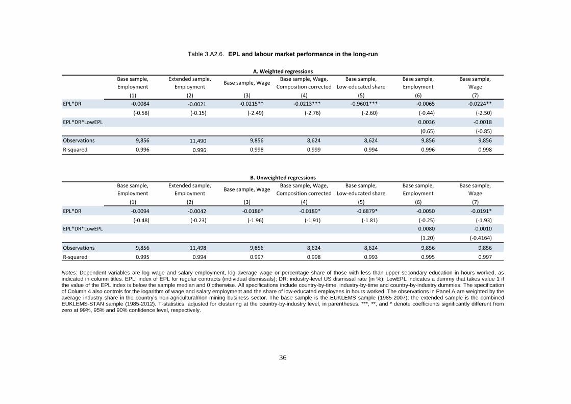
36

Table 3.A2.6. EPL and labour market performance in the long-run

Notes: Dependent variables are log wage and salary employment, log average wage or percentage share of those with less than upper secondary education in hours worked, as indicated in column titles. EPL: index of EPL for regular contracts (individual dismissals); DR: industry-level US dismissal rate (in %); LowEPL indicates a dummy that takes value 1 if the value of the EPL index is below the sample median and 0 otherwise. All specifications include country-by-time, industry-by-time and country-by-industry dummies. The specification of Column 4 also controls for the logarithm of wage and salary employment and the share of low-educated employees in hours worked. The observations in Panel A are weighted by the average industry share in the country’s non-agricultural/non-mining business sector. The base sample is the EUKLEMS sample (1985-2007); the extended sample is the combined EUKLEMS-STAN sample (1985-2012). T-statistics, adjusted for clustering at the country-by-industry level, in parentheses. ***, **, and * denote coefficients significantly different from zero at 99%, 95% and 90% confidence level, respectively.

Base sample,

Employment

Extended sample,

EmploymentBase sample, Wage

Base sample, Wage,

Composition corrected

Base sample,

Low-educated share

Base sample,

Employment

Base sample,

Wage

(1) (2) (3) (4) (5) (6) (7)

EPL*DR -0.0084 -0.0021 -0.0215** -0.0213*** -0.9601*** -0.0065 -0.0224**

(-0.58) (-0.15) (-2.49) (-2.76) (-2.60) (-0.44) (-2.50)

EPL*DR*LowEPL 0.0036 -0.0018

(0.65) (-0.85)

Observations 9,856 11,490 9,856 8,624 8,624 9,856 9,856

R-squared 0.996 0.996 0.998 0.999 0.994 0.996 0.998

Base sample,

Employment

Extended sample,

EmploymentBase sample, Wage

Base sample, Wage,

Composition corrected

Base sample,

Low-educated share

Base sample,

Employment

Base sample,

Wage

(1) (2) (3) (4) (5) (6) (7)

EPL*DR -0.0094 -0.0042 -0.0186* -0.0189* -0.6879* -0.0050 -0.0191*

(-0.48) (-0.23) (-1.96) (-1.91) (-1.81) (-0.25) (-1.93)

EPL*DR*LowEPL 0.0080 -0.0010

(1.20) (-0.4164)

Observations 9,856 11,498 9,856 8,624 8,624 9,856 9,856

R-squared 0.995 0.994 0.997 0.998 0.993 0.995 0.997

A. Weighted regressions

B. Unweighted regressions

37

63. By contrast, the degree of stringency of EPL is found to have a negative long-run association

with average wages, which is robust to the choice of the estimator and to controlling for the composition of

employment – by including log employment and the share of the low-skilled in the vector of covariates.

This result, which is robust to exclusion of countries one-by-one from the sample (Figure 3.A2.4, Panel B),

appears consistent with the finding of a negative relationship between firing restrictions and productivity

reported in the literature (see OECD, 2013, for a survey). Interestingly, the degree of stringency of

EPL appears also to foster relative employment of the low-educated in the long-run, even if the effect is

quantitatively small.

Figure 3.A2.4. Long-run effects of flexibility-enhancing EPL reforms, employment and wages: Robustness to varying the country sample

Estimated coefficient

Notes: The chart reports point estimates and 90%-confidence intervals of the coefficient of EPL in col. 1 (Panel A) and 3 (Panel B) of Panel A of Table 3.A1.6 for employment and wages, respectively. Each dot indicates the coefficient estimated dropping from the sample the country indicated on the X-axis. Estimates are obtained by assuming that, in each industry, the impact of EPL is greater, the greater the US dismissal rate in that industry. Confidence intervals are obtained by clustering errors on countries and industries.

Source: OECD estimates based on EUKLEMS and OECD EPL Databases.

-0.06

-0.04

-0.02

0

0.02

0.04

0.06

KOR AUS IRL ITA AUT HUN CZE SVK CAN DNK NLD GRC SWE JPN POL BEL FIN FRA DEU GBR PRT ESP

A. Wage and salary employment

All countries

-0.07

-0.06

-0.05

-0.04

-0.03

-0.02

-0.01

0

ESP GBR FRA AUT ITA PRT BEL JPN SVK IRL CAN NLD SWE CZE DNK HUN POL DEU FIN GRC KOR AUS

B. Average hourly wages (composition corrected)

All countries

38

64. Bèlot et al. (2007) suggests that, from a growth perspective, the optimal level of employment

protection is strictly positive since excessively lax regulations can reduce employees’ incentives to invest in

firm-specific knowledge. On the basis of their theoretical work, one could therefore expect to find a positive

long-run impact of dismissal regulations on either employment or wages in countries where these regulations

are less stringent. A simple way to investigate this issue is to allow the effect of EPL to differ on the basis of

its level, by allowing a structural break at the median of the sample. Columns 6 and 7 of Table 3.A2.6 show

that the long-run impact of EPL on both employment and wages does not differ between high and low levels

of EPL stringency.

3. Regression-discontinuity models

3.1. Data and estimation methodology

65. This section provides additional evidence on the short-term effects of structural reforms by

considering three case studies concerning recent labour market reforms in Estonia (July 2009),

Spain (February 2012) and Slovenia (April 2013). More precisely, the estimation strategy is conceived

to identify the joint effect of all the provisions included in each reform by comparing labour market

performance before and after the date of enforcement. Two performance variables are examined:

the seasonally-adjusted standardised unemployment rate and the share of open-ended contracts in

new contracts (new hires plus conversions). The key identification assumption is that, conditional on

control variables included in the model, labour market performance evolves in a smooth way, so that any

discontinuous jump in performance on the date of the labour market reform can be attributed to it (and

other institutional changes occurring simultaneously). In order to properly isolate the effect of the reform

from that of the business cycle (which is key for the validity of the smoothness assumption), the estimation

models include a number of aggregate covariates and, most importantly, polynomial time trends up to the

5th order. Following standard practice (see e.g. Imbens and Lemieux, 2008; Lee and Card, 2008),

polynomial trends are allowed to differ before and after the reform. The general regression-discontinuity

model, which is estimated on monthly data, can be written as:

tt

s

s

Rts

s

s

sRttt DRtIRtIYP

5

1

5

1

)()( (4)

where P is the performance variable (unemployment rate or share of permanent contracts) at time t, R is the

date of the reform, I is the indicator function (which equals 1 after the reform and 0 before), D stands for

monthly dummies, and Greek letters stand for parameters to be estimated, except for , which represents

a standard error term. Y is a vector of aggregate confounding factors. These include the logarithms of the

industrial production and real turnover in the retail sector when the unemployment rate is the dependent

variable. By contrast, when the share of open-ended contracts is the dependent variable, Y includes the

level and change in the unemployment rate and the share of youth and older workers in new contracts.

66. The parameter of interest is . A significant estimate for this parameter suggests a significant

impact of the reform.

67. Obviously, misspecification of the empirical model might lead to identify a discontinuous shift

in performance around the date of a reform even when this shift occurs before the reform (and cannot

therefore be attributed to it). To validate the empirical model, in the light of this possibility, placebo tests

are run by fictitiously setting the value of R to some date preceding the reform (but sufficiently close to it).

If discontinuous shifts in performance are really induced by the reform, then no effect should be found at

these anticipated dates.

68. A second issue concerns possible manipulations around the threshold. For example, if the

reduction in firing costs were anticipated, employers could delay firing to the post-enactment period in

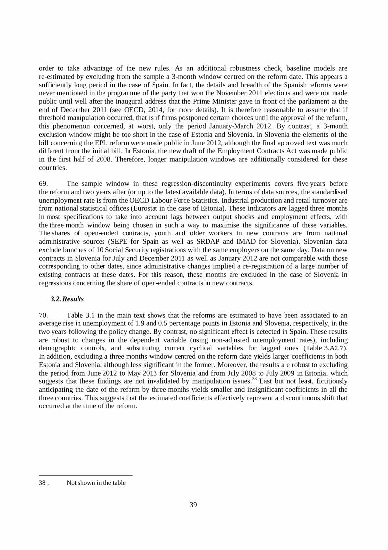
39

order to take advantage of the new rules. As an additional robustness check, baseline models are

re-estimated by excluding from the sample a 3-month window centred on the reform date. This appears a

sufficiently long period in the case of Spain. In fact, the details and breadth of the Spanish reforms were

never mentioned in the programme of the party that won the November 2011 elections and were not made

public until well after the inaugural address that the Prime Minister gave in front of the parliament at the

end of December 2011 (see OECD, 2014, for more details). It is therefore reasonable to assume that if

threshold manipulation occurred, that is if firms postponed certain choices until the approval of the reform,

this phenomenon concerned, at worst, only the period January-March 2012. By contrast, a 3-month

exclusion window might be too short in the case of Estonia and Slovenia. In Slovenia the elements of the

bill concerning the EPL reform were made public in June 2012, although the final approved text was much

different from the initial bill. In Estonia, the new draft of the Employment Contracts Act was made public

in the first half of 2008. Therefore, longer manipulation windows are additionally considered for these

countries.

69. The sample window in these regression-discontinuity experiments covers five years before

the reform and two years after (or up to the latest available data). In terms of data sources, the standardised

unemployment rate is from the OECD Labour Force Statistics. Industrial production and retail turnover are

from national statistical offices (Eurostat in the case of Estonia). These indicators are lagged three months

in most specifications to take into account lags between output shocks and employment effects, with

the three month window being chosen in such a way to maximise the significance of these variables.

The shares of open-ended contracts, youth and older workers in new contracts are from national

administrative sources (SEPE for Spain as well as SRDAP and IMAD for Slovenia). Slovenian data

exclude bunches of 10 Social Security registrations with the same employers on the same day. Data on new

contracts in Slovenia for July and December 2011 as well as January 2012 are not comparable with those

corresponding to other dates, since administrative changes implied a re-registration of a large number of

existing contracts at these dates. For this reason, these months are excluded in the case of Slovenia in

regressions concerning the share of open-ended contracts in new contracts.

3.2. Results

70. Table 3.1 in the main text shows that the reforms are estimated to have been associated to an

average rise in unemployment of 1.9 and 0.5 percentage points in Estonia and Slovenia, respectively, in the

two years following the policy change. By contrast, no significant effect is detected in Spain. These results

are robust to changes in the dependent variable (using non-adjusted unemployment rates), including

demographic controls, and substituting current cyclical variables for lagged ones (Table 3.A2.7).

In addition, excluding a three months window centred on the reform date yields larger coefficients in both

Estonia and Slovenia, although less significant in the former. Moreover, the results are robust to excluding

the period from June 2012 to May 2013 for Slovenia and from July 2008 to July 2009 in Estonia, which

suggests that these findings are not invalidated by manipulation issues.38

Last but not least, fictitiously

anticipating the date of the reform by three months yields smaller and insignificant coefficients in all the

three countries. This suggests that the estimated coefficients effectively represent a discontinuous shift that

occurred at the time of the reform.

38 . Not shown in the table

40

Table 3.A2.7. Recent EPL reforms and unemployment: sensitivity analysis

Estimated average effect within two years from the reform in percentage points

Notes: The dependent variable is the seasonally-adjusted standardised unemployment rate. Estimates based on regression-discontinuity models fitted on monthly data. Each specification controls for the 3-month-lagged industrial production and retail turnover indexes, a 5

th order polynomial time trend (heterogeneous between the pre- and post-reform period) and month

dummies, except when differently indicated. Reform nsa: Dependent variable not adjusted for seasonality. Reform demogr cntrls: Share of youth and of women in labour force included. Reform curr cntrls: Indexes of retail turnover and industrial production included as contemporaneous variables. Reform no manipulation: Exclusion from the sample of three months around the reform date. Placebo 3 months: Fictitious reform 3 months before the true reform. Robust t-statistics are in brackets. ***, **, * statistically significant at 1%; 5% and 10% levels respectively.

71. Table 3.2 in the main text reports the estimated effects of the reforms on the share of open-ended

contracts in new contracts. Based on these results, the reforms increased this share by 10.8 and

3.1 percentage points in Slovenia and Spain, respectively.39

Table 3.A2.8 shows that excluding a 3-months

window centred on the reform date yields a smaller coefficient in Slovenia and a larger one in Spain.

But both remain significant at least at the 5% statistical level. Moreover, the coefficient for Slovenia also

remains significant if the period from June 2012 to May 2013 is excluded from the sample. 40

In addition,

fictitiously anticipating the date of the reform by 3 months yields insignificant coefficients of opposite sign

in both countries.

39 . Data on new contracts are unavailable in the case of Estonia.

40 . Not shown in the table

(1) (2) (3) (4) (5)

reform nsareform demogr

cntrls

reform curr

cntrls

reform no

manipulation

placebo 3

months

Estimated average effect

(% points) 2.57** 1.69*** 1.85*** 1.97* 1.22

(2.32) (2.83) (2.76) (1.76) (1.19)

Observations 84 84 84 81 84

R-squared 0.991 0.996 0.995 0.996 0.994

(1) (2) (3) (4) (5)

reform nsareform demogr

cntrls

reform curr

cntrls

reform no

manipulation

placebo 3

months

Estimated average effect

(% points) 1.11*** 0.50* 0.62* 1.33* -0.04

(2.83) (1.78) (1.89) (1.95) (-0.13)

Observations 84 84 84 81 84

R-squared 0.987 0.991 0.989 0.990 0.989

(1) (2) (3) (4) (5)

reform nsareform demogr

cntrls

reform curr

cntrls

reform no

manipulation

placebo 3

months

Estimated average effect

(% points) 0.34 0.26 -0.29 -0.65 -0.42

(0.49) (0.43) (-0.53) (-0.63) (-0.97)

Observations 84 84 84 81 84

R-squared 0.996 0.997 0.998 0.997 0.997

A. Estonia

B. Slovenia

C. Spain

41

Table 3.A2.8. Recent EPL reforms and share of permanent contracts in new contracts: sensitivity analysis

Estimated average effect within two years from the reform in percentage points

Notes: The dependent variable is the share of permanent contracts in new contracts. Estimates based on regression-discontinuity models fitted on monthly data. Each specification controls for level and changes in the standardised unemployment rate, the share of youth and older workers in new contracts, a fifth order polynomial time trend (heterogeneous between the pre- and post-reform period) and month dummies. The specification for Slovenia excludes data for July, December and January of each year, except where differently specified. Reform no manipulation: Exclusion from the sample of three months around the reform date. Placebo three months: Fictitious reform three months before the true reform. All months: July, December and January included in the sample (except for July to December 2011, and January 2012). Robust t-statistics are in parentheses. ***: statistically significant at the 1% level.

72. In the baseline model for Slovenia, observations for July, December and January of each year are

excluded from the sample, to avoid that missing values bias the estimates of month dummies. However, as

discussed above, data on new contracts for these months are available and reliable except for July and

December 2011 as well as January 2012. The last column of Table 3.A2.8 shows that the results are robust

to the inclusion of January, July and December in the sample.

4. Difference-in-difference analysis of the 2009 Estonian reform

4.1. Data and estimation methodology

73. In the case of the Estonian reform additional evidence on its impact on unemployment

is provided here on the basis of a difference-in-difference model estimated on individual data from

the Quarterly European Labour Force Survey and using other Baltic countries as a control group, as

suggested by Malk (2013). In particular, Lithuania appears to be a suitable control group: both countries

are small open-economies with the same trading partners; they display a similar evolution of real GDP,

industrial production and retail turnover before and after July 2009 (see Figure 3.A2.5); before the

Estonian reform they were characterised by outstandingly similar trends in unemployment as well as stocks

and flows of temporary contracts (see Figure 3.11 and 3.12 in the main text); and no significant changes in

labour market policies and institutions occurred in Lithuania in this period.

Reform no

manipulation

Placebo 3

monthsAll months

8.14** -2.06 12.21***

(2.63) (-0.51) (6.25)

Observations 60 63 77

R-squared 0.93 0.873 0.918

Reform no

manipulation

Placebo 3

months

5.73*** -0.96

(6.68) (-1.55)

Observations 81 84

R-squared 0.983 0.975

A. Slovenia

B. Spain

Estimated coefficient

(% points)

Estimated coefficient

(% points)

42

Figure 3.A2.5. Evolution of the economic activity in Estonia and Lithuania, Q3 2004-Q2-2011

Quarterly percentage changes, seasonally-adjusted

Notes: The vertical line indicates the date of enforcement of the Estonian labour market reform (July 1st, 2009, that is at the beginning

of Q3 2009).

Source: Eurostat.

0

5

10

15

20

25

-15

-10

-5

0

5

A. Real GDP growth

Estonia Lithuania

EPL reform in Estonia: 1st July 2009

0

5

10

15

20

25

-20

-15

-10

-5

0

5

10

B. Growth of the industrial production index

Estonia Lithuania

EPL reform in Estonia: 1st July 2009

0

2

4

6

8

10

12

14

16

18

20

-15

-10

-5

0

5

10

C: Growth of the index of retail turnover (deflated)

Estonia Lithuania

EPL reform in Estonia: 1st July 2009

43

74. The effect of the Estonian reform is estimated through a difference-in-difference probit model in

which the probability of being unemployed in a given month is a function of a large set of individual and

aggregate covariates and is allowed to diverge between Lithuania and Estonia in the aftermath of the

Estonian reform. Formally the probability of being unemployed of individual i in country c at time t is

modelled as:

𝑃𝑟𝑜𝑏(𝑈𝑖𝑐𝑡 = 1) = 𝐹(𝛼 + 𝑋𝑐𝑖𝑡𝛽1 + 𝑌𝑐𝑡𝛽2 + 𝛾𝐼𝑡>𝑅 + 𝛿𝐷𝐸𝑆𝑇 + 𝜃𝐷𝐸𝑆𝑇𝐼𝑡>𝑅 + 𝜈𝑡). (5)

where F is the Normal cumulative distribution function, X is a vector of individual controls (including

gender, 3 educational attainment classes, 15 age classes, 3 classes for the degree of urbanisation, a dummy

for being born in the country of residence, and 23 classes for the duration of residence in the country if

foreign born), Y is a vector of aggregate controls (including the 3-month-lagged changes in industrial

production and retail turnover indexes, month dummies, and, in a sensitivity analysis, a 5th-order

polynomial time trend),41

I stands for the indicator function denoting the post-July 2009 period, D is a

country dummy for Estonia and 𝜈 are dummies for the calendar month of the reference week. The

parameter of interest is 𝛿. A significantly positive estimated value for this parameter would suggest a

positive impact of the Estonian reform on unemployment. When Latvia is included, an additional country

dummy for Latvia is added. The sample window is restricted to individuals in the labour force and to

two years before and after the date of enforcement of the Estonian reform. Cross-section probability

weights are used.

4.2. Results

75. Baseline difference-in-difference estimates of the effect of the reform (Table 3.A2.9) are

remarkably close to those obtained using the regression-time discontinuity model discussed in the previous

section. Conditional on included controls, the probability of being unemployed is estimated to be, on

average, 1.5 percentage points higher in the two years following the reform. This is a somewhat larger

number than what can be estimated by simple comparison of unemployment patterns in Estonia and

Lithuania without controls (see Figure 3.12 in the main text), which might be due to the fact that the

Lithuanian business-cycle seems to follow the Estonian one by about one quarter (see Figure 3.A2.5).

Adding Latvia to the control group or including a polynomial time trend increases both the point-estimate

and significance.42

41. When included, the time trend is allowed to be different before and after the reform date. After the reform

date is also allowed to differ between Estonia and Lithuania.

42. The same result occurs if contemporaneous indexes of industrial production and retail turnover are

included to replace lagged ones. Also, if the effect is allowed to vary between the first and the second

post-reform period, all the significant effect on unemployment is concentrated in the first year. Both these

results are not shown in the table.

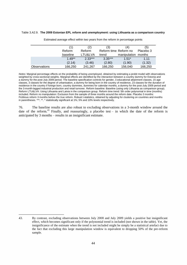
44

Table 3.A2.9. The 2009 Estonian EPL reform and unemployment: using Lithuania as a comparison country

Estimated average effect within two years from the reform in percentage points

Notes: Marginal percentage effects on the probability of being unemployed, obtained by estimating a probit model with observations weighted by cross-sectional weights. Marginal effects are identified by the interaction between a country dummy for Estonia and a dummy for the post-July 2009 period. The baseline specification controls for gender, 3 educational attainment classes, 15 age classes, 3 classes for the degree of urbanisation, a dummy for being born in the country of residence, 23 classes for the duration of residence in the country if foreign born, country dummies, dummies for calendar months, a dummy for the post-July 2009 period and the 3-month-lagged industrial production and retail turnover. Reform baseline: Baseline (using only Lithuania as comparison group). Reform LTU&LVA: Using Lithuania and Latvia in the comparison group. Reform time trend: 5th order polynomial in time (months) included. Reform no manipulation: Exclusion from the sample of three months around the reform date. Placebo 3 months: Fictitious reform 3 months before the true reform. Robust t-statistics, obtained by adjusting for clustering on countries and months in parentheses. ***, **, * statistically significant at 1%; 5% and 10% levels respectively.

76. The baseline results are also robust to excluding observations in a 3-month window around the

date of the reform.43

Finally, and reassuringly, a placebo test – in which the date of the reform is

anticipated by 3 months – results in an insignificant estimate.

43. By contrast, excluding observations between July 2008 and July 2009 yields a positive but insignificant

effect, which becomes significant only if the polynomial trend is included (not shown in the table). Yet, the

insignificance of the estimate when the trend is not included might be simply be a statistical artefact due to

the fact that excluding this large manipulation window is equivalent to dropping 50% of the pre-reform

sample.

(1) (2) (3) (4) (5)Reform

baseline

Reform

LTU&LVA

Reform time

trend

Reform no

manipulation

Placebo 3

months

1.49** 2.33*** 3.35*** 1.51* 1.11

(2.14) (3.46) (2.80) (1.90) (1.32)

Observations 166,250 241,267 166,250 156,040 166,250

45

References

Bassanini, A. and R. Duval (2009), “Unemployment, Institutions, and Reform Complementarities:

Re-assessing the Aggregate Evidence for OECD Countries”, Oxford Review of Economic Policy,

Vol. 25, pp. 40-59.

Bassanini, A. and A. Garnero (2013), “Dismissal Protection and Worker Flows in OECD Countries:

Evidence from Cross-country/Cross-industry Data”, Labour Economics, Vol. 21, pp. 25-41.

Bassanini, A., L. Nunziata and D. Venn (2009), “Job Protection Legislation and Productivity Growth in

OECD Countries”, Economic Policy, Vol. 58, pp. 349-402.

Bélot, M., J. Boone and J. Van Ours, J. (2007), “Welfare-Improving Employment Protection”, Economica,

Vol. 74, pp 381–396.

Blanchard, O. and J. Wolfers (2000), “The Role of Shocks and Institutions in the Rise of European

Unemployment: The Aggregate Evidence”, The Economic Journal, Vol. 110, No. 462, pp. C1-C33.

Card, D. and S. Lee (2008), "Regression discontinuity inference with specification error," Journal of

Econometrics, Vol. 142 No. 2, pp. 655-674.

Imbens, G.W., and T. Lemieux (2008), "Regression discontinuity design: A guide to practice" Journal of

Econometrics, vol. 142(2), pp. 615-635.

Gal, P.N. and A. Theising (2015), “The Macroeconomic Impact of Structural Policies on Labour Market

Outcomes in OECD countries: A Reassessment”, OECD Economics Department Working Papers,

No. 1271, OECD Publishing, Paris, http://dx.doi.org/10.1787/5jrqc6t8ktjf-en.

Jordà, O. (2005), Estimation and inference of impulse responses by local projections, American Economic

Review, Vol. 95, No. 1, pp. 161–182.

Malk, L. (2013), "Relaxation of employment protection and its effects on labour reallocation," Bank of

Estonia Working Papers wp2013-4, Bank of Estonia.

Nickell, S., L. Nunziata and W. Ochel (2005), “Unemployment in the OECD Since the 1960s: What Do

We Know?”, The Economic Journal, Vol. 115, pp. 1-27.

OECD (2012), Employment Outlook, OECD Publishing, Paris, http://dx.doi.org/10.1787/empl_outlook-2012-en.

OECD (2013), Employment Outlook, OECD Publishing, Paris, http://dx.doi.org/10.1787/empl_outlook-2013-en.

OECD (2014), The 2012 Labour Market Reform in Spain: A Preliminary Assessment, OECD Publishing, Paris,

http://dx.doi.org/10.1787/9789264213586-en.

Teulings, C. and N. Zubanov (2014), “Is Economic Recovery a Myth? Robust Estimation of Impulse

Responses”, Journal of Applied Econometrics, vol. 29, pp. 497-514.

46

Zweimüller, J. (2009); “Comments to ‘Job Protection Legislation and Productivity Growth in

OECD Countries’”, Economic Policy, Vol. 58.

47

ANNEX 3.A3 INDICATORS OF REGULATION IN PRODUCT AND LABOR MARKETS

Table 3.A3.1. Anti-competitive regulation in network industries across OECD countries, 2013

Scale from 0 (least restrictions) to 6 (most restrictions)

Note: Simple averages of the indicators of barriers to entry and (when available) vertical integration in Electricity and Gas (Energy), Air, Rail and Road transport (Transport), Post and Telecoms (Communications). Data refer to 2008 for the United States. Regulation data in Gas and Rail are not available in the case of Iceland.

Source: OECD Product Market Regulation Statistics (database). DOI: http://dx.doi.org/10.1787/f33213b2-en.

Energy Transport Communications

Austra l ia 2.9 0.8 1

Austria 2.2 1.9 0

Belgium 2.1 2.6 0

Canada 2.6 2.4 0.5

Chi le 3.2 1.9 1.25

Czech Republ ic 2.3 1.9 0

Denmark 2.2 1.5 0

Estonia 1.8 1.9 0

Finland 3.3 2.5 0

France 2.3 3.0 0

Germany 2.3 1.5 0

Greece 2.4 2.6 0

Hungary 2.1 2.3 0

Iceland 3.1 2.3 1

Ireland 1.9 2.6 0

Israel 2.4 3.9 1.75

Ita ly 2.2 2.4 0.5

Japan 3.2 2.8 0.5

Korea 4.3 3.4 0.5

Luxembourg 2.8 3.4 0

Mexico 4.6 4.3 1.75

Netherlands 2.4 2.4 0

New Zealand 2.5 3.8 0

Norway 3.6 2.0 0.5

Poland 2.6 2.4 0

Portugal 1.2 2.4 0.5

Slovak Republ ic 2.2 2.0 0

Slovenia 2.2 3.1 0

Spain 1.5 2.9 0

Sweden 1.7 1.5 0

Switzerland 3.2 2.0 0.5

Turkey 2.7 5.0 1

United Kingdom 1.2 1.0 0

United States 3.1 3.1 1

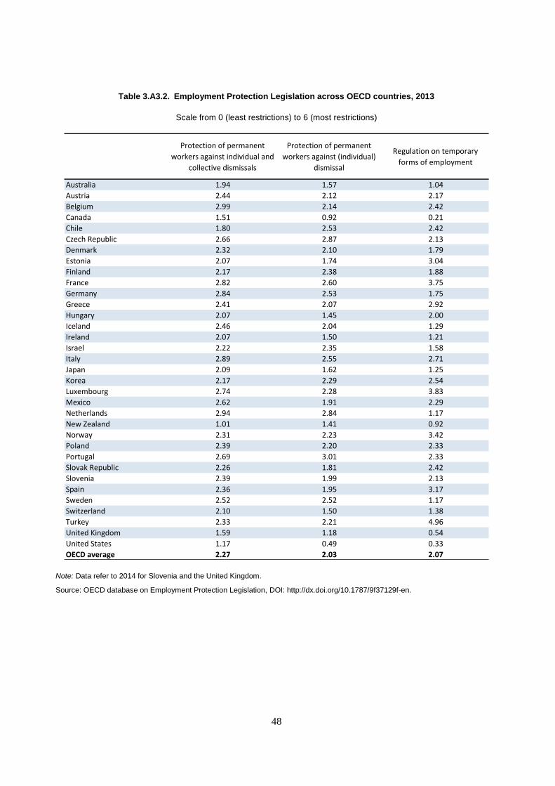
48

Table 3.A3.2. Employment Protection Legislation across OECD countries, 2013

Scale from 0 (least restrictions) to 6 (most restrictions)

Note: Data refer to 2014 for Slovenia and the United Kingdom.

Source: OECD database on Employment Protection Legislation, DOI: http://dx.doi.org/10.1787/9f37129f-en.

Protection of permanent

workers against individual and

collective dismissals

Protection of permanent

workers against (individual)

dismissal

Regulation on temporary

forms of employment

Australia 1.94 1.57 1.04

Austria 2.44 2.12 2.17

Belgium 2.99 2.14 2.42

Canada 1.51 0.92 0.21

Chile 1.80 2.53 2.42

Czech Republic 2.66 2.87 2.13

Denmark 2.32 2.10 1.79

Estonia 2.07 1.74 3.04

Finland 2.17 2.38 1.88

France 2.82 2.60 3.75

Germany 2.84 2.53 1.75

Greece 2.41 2.07 2.92

Hungary 2.07 1.45 2.00

Iceland 2.46 2.04 1.29

Ireland 2.07 1.50 1.21

Israel 2.22 2.35 1.58

Italy 2.89 2.55 2.71

Japan 2.09 1.62 1.25

Korea 2.17 2.29 2.54

Luxembourg 2.74 2.28 3.83

Mexico 2.62 1.91 2.29

Netherlands 2.94 2.84 1.17

New Zealand 1.01 1.41 0.92

Norway 2.31 2.23 3.42

Poland 2.39 2.20 2.33

Portugal 2.69 3.01 2.33

Slovak Republic 2.26 1.81 2.42

Slovenia 2.39 1.99 2.13

Spain 2.36 1.95 3.17

Sweden 2.52 2.52 1.17

Switzerland 2.10 1.50 1.38

Turkey 2.33 2.21 4.96

United Kingdom 1.59 1.18 0.54

United States 1.17 0.49 0.33

OECD average 2.27 2.03 2.07