Shipboard Integrated Sensors and Weapons Systems...

Shipboard Integrated Sand Weapons Systems(SISWS)

Calculation of Required Population SizeConfidence and Accuracy of Results

27 April 2004

Prepared for DRDC-Ottawa 3701 Carling Avenue Ottawa, Ontario K1A 0Z4

Prepared by Sky Industries Inc. 2956 McCarthy Rd. Ottawa ON Canada K1V 8K6

Submitted by Lockheed Martin Canada Inc. 3001 Solandt Rd. Kanata, Ontario K2K 2M8

Approved by R. Martelli

1010858, Revision 1 Copyright © 2004 Her Majesty the Queen in Right of Canada

DRDC Ottawa CR 2004 - 001

ensors

for Desired

1010858, Rev. 1 A

The use or disclosure of the data on this sheet is subject to the restrictions on the title page of this document.

LIST OF EFFECTIVE PAGES

Total number of pages in this document is 27, consisting of the following:

Page Number Revision Level

Title 1 A 1 i to ii 1

1 to 24 1

1010858, Rev. 1 i


REVISION RECORD

REVISION NO.

AFFECTED PAGES

DESCRIPTION ISSUE DATE INITIAL

1 All Initial release 27 April 2004

1010858, Rev. 1 ii


TABLE OF CONTENTS

Paragraph Title Page

1. INTRODUCTION ............................................................................................................ 1

2. REFERENCES.................................................................................................................. 2

3. PDF OF STATISTICALLY INDEPENDENT MONTE-CARLO RUNS ................... 2

4. PDF QUANTIZATION BY POPULATION SIZE........................................................ 5

5. CONFIDENCE AND ACCURACY FOR BOUNDED PS VALUES............................ 9

6. APPLICATIONS ............................................................................................................ 11 6.1 Effect of Population Consistency on Required Population Size....................................... 11 6.2 Choosing Population Size ................................................................................................. 15 6.3 Interpretation of A Priori Populations............................................................................... 17

7. EXTENSION TO CONTINUOUS VARIABLES........................................................ 19

8. CONCLUSION ............................................................................................................... 24

LIST OF ILLUSTRATIONS

Figure Title Page

Figure 1 Probability Density Functions for Binomial Random Variable.......................................... 5 Figure 2 Effect of PDF Quantization on Probability that Ps is Estimated to a Given Accuracy ....... 7 Figure 3 Probability Curves Extended to Population Size of 250 Runs............................................ 8 Figure 4 Confidence Curves for Bounded Ps, 40% < Ps <80% ....................................................... 10 Figure 5 Confidence Curves for Various Ground-truth Ps Ranges ................................................. 13 Figure 6 Consistency of Simulation Results Increases Confidence for Fixed Population Size ...... 14 Figure 7 Illustration of Tradeoff between Accuracy and Confidence of Estimated Ps ................... 15 Figure 8 Example for Selection of Run Population Size................................................................. 16 Figure 9 Example for Interpretation of Estimated Ps based on Population Size ............................. 18 Figure 10 Confidence Curves for Analysis of Miss Distance Statistics............................................ 21 Figure 11 Probability Range Bins for Minimum Miss Distance....................................................... 22 Figure 12 90% Confidence Envelope for Observing Minimum Miss Distance in Run Population.. 23

1010858, Rev. 1 1


1. INTRODUCTION

Consider the problem of using software simulation or hardware experiments (“trials”) to determine the effectiveness of an Electronic Countermeasure (ECM) in protecting a surface ship against a missile attack. Software simulation of a missile attack against a jammer equipped ship can be used to estimate the effectiveness of a particular ECM technique, waveform, or ploy. In order to reflect the principal features of a missile attack and corresponding ship defense, the software models are required to include a large number of nonlinear processes, and as a result the outcome of the simulation can depend heavily on initial conditions and missile/scenario/ECM parameters used in a single run. Under certain conditions, small changes in the values chosen for simulation parameters can change the outcome of a simulated missile attack from a miss to a hit or vice versa. For this reason, the predictive power of missile engagement software models in general can be reasonably questioned, and the predictive power of a single simulation run is especially suspect. The situation is exacerbated by the fact that the selection of model parameters is generally based on incomplete, uncertain, and inconsistent information because (a) intelligence information about missile characteristics and design may be uncertain or lacking altogether, and (b) specifics of the attack scenario such as launch range, seeker activation range, approach bearing, and environmental conditions are not determined until the instant of the attack. Difficulties related to parameter selection are endemic to this work. As a consequence, a software model cannot be used on a single-run basis to confidently predict the effectiveness of a candidate ECM technique, waveform or ploy in preventing a missile intercept. Instead, the software model is best used in a manner that exposes its statistical behavior. This requires that the model be used to create a population of data. The predictive power of the model, in terms of a chosen Measure Of Merit (MOM) is vested in the statistical characteristics of the data population. In order to realize this predictive power, the relationships between population size, variability of results, and confidence of results distilled from the population must be quantitatively determined.

The purpose of this report is to describe a quantitative mathematical foundation for the following:

a. Calculate the required number of simulation runs or trials in order to determine the ECM effectiveness to a desired accuracy and confidence

b. Determine the accuracy of the ECM effectiveness as calculated from a population of simulation runs or trials, based on the run population size

c. Determine the confidence level of the ECM effectiveness, based on the run population size.

Although the analysis presented here applies equally to software simulation and hardware trials, the term “simulation runs” shall be used to refer equally to software simulation and hardware trials.

For the purposes of this analysis, ECM effectiveness is defined as the probability that a surface ship will survive a missile attack if the countermeasure is deployed. For the purposes of this analysis and discussion, the term “ship survival” is defined as failure of the missile to hit the ship.

If simulation runs are statistically independent, then the outcome of n runs is analogous to tossing an unfair coin n times. The problem of determining ECM effectiveness is equivalent to determining the probability that the ship will avoid being hit during the missile attack, which is equivalent to determining

1010858, Rev. 1 2


the bias in the coin. Like the random variable representing the outcome of coin tosses, the outcome of simulation runs (missile hit or missile miss) is a binomial random variable [1]. This analysis and discussion applies only to data analysis involving MOMs which are binomial random variables, i.e. MOMs which assume one of only two possible values. Other MOMs, such as those which are continuously variable (e.g., missile miss distance) must be treated differently or converted to a binomial random variable as described in Section 7.

2. REFERENCES

[1] Eisen, Carole and Eisen, Martin; Probability and Its Applications; Quantum Publishers Inc., 257 Park Avenue South, New York, New York 10010, ©1975

3. PDF OF STATISTICALLY INDEPENDENT MONTE-CARLO RUNS

Given n statistically independent simulation runs and a binary definition of success or failure, there are a countable number of population “outcomes”, where a population outcome is defined as an unique sequence of successes and failures. For example, if 3 simulation runs are performed, then irrespective of ECM effectiveness there are 23 = 8 possible outcomes after the 3 runs have been completed. Table 1 lists the possible outcomes, where “HIT” refers to a simulation run in which the missile hit the ship, and “MISS” refers to a simulation run in which the missile missed the ship.

Table 1

Simulation Run 1 Simulation Run 2 Simulation Run 3 No. of Misses Population 1 HIT HIT HIT 0 Population 2 MISS HIT HIT 1 Population 3 HIT MISS HIT 1 Population 4 HIT HIT MISS 1 Population 5 MISS MISS HIT 2 Population 6 HIT MISS MISS 2 Population 7 MISS HIT MISS 2 Population 8 MISS MISS MISS 3

Let Ps represent the true probability of ship survival, where the term “ship survival” is defined as failure of the missile to hit the ship. The probability of observing m misses in n simulation runs is given by the following expression:

1010858, Rev. 1 3


P(m misses i n n trials) = n Cm (Ps)m(1 - Ps)n-m

Equation 1

where

n Cm = )!(!

!mnm

n−

n!

Equation 2

The Probability Density Function (PDF) expressed in Equation 1 and Equation 2 is a function of the true probability of ship survival, Ps, and the number simulation runs, n. Graphs of the PDF are presented in fig. A (a), for values of Ps from 10% to 90%, for 25, 50, and 100 simulation runs.

Referring to Figure 1 (a), as the number of simulation runs becomes larger, the probability of observing any particular outcome becomes smaller because there is a greater number of possible outcomes, and the sum of the probabilities of all possible outcomes is 1.0, i.e. the curve encompasses all possible outcomes (see Figure 1 (b), illustrating a Riemann sum of the area under the PDF curve). However, as the number of runs in the population increases, the accuracy with which the true value of Ps can be determined increases. This can be understood intuitively by considering the following three cases:

Case 1: Ps = 50%, population of 100 simulation runs

The possible outcomes near Ps = 50% are 48%, 49%, 50%, 51%, 52%; no other possibilities exist. Because the population is limited to 100 runs and the outcome of each run is a binary value (hit or miss, like a coin toss), it is not possible to observe values intermediate between those listed above, e.g. Ps = 51.6%.


The possible outcomes near Ps = 50% are 11, 12, 13, 14 misses in a population of 25 runs, corresponding to estimated Ps values of 44%, 48%, 52%, and 56% respectively. No other possibilities exist. Because the population is limited to 25 runs and the outcome of each run is a binary value (hit or miss, like a coin toss), it is not possible to observe values intermediate between those listed above, e.g. Ps = 50% is not a possible outcome.


The possible outcomes near Ps = 50% are 5, 6, 7, 8 misses in a population of 13 runs, corresponding to estimated Ps values of 38.5%, 46.2%, 53.8%, and 61.5% respectively. No intermediate possibilities exist for a population of 13 runs.

1010858, Rev. 1 4


0 20% 40% 60% 80% 100%0

0.05

0.1

0.15

0.2

0.25

0.3

0.35

Percentage of misses in n simulation runs

P = 10%s

P = 20%s

P = 30%sP = 40%s P = 50%s

P = 60%sP = 70%s

P = 80%s

P = 90%s

Pro

babi

lity

of o

bser

ving

X%

mis

ses

in n

sim

ulat

ion

runs

n = population of 25 simulation runsn = population of 50 simulation runsn = population of 100 simulation runs

P = 50%s

0 20% 40% 60% 80% 100%0

0.05

0.1

0.15

0.2

0.25

0.3

0.35

Percentage of misses in n simulation runs

Prob

abilit

y of

obs

ervi

ng X

% m

isse

s in

n s

imul

atio

n ru

ns

P5

P9

P10

P12

P14P15P1

P2

P3

P4

P6

P7

P8

P11

P13

P = 50%si = 1

15

Pi = 1.0

(a) binomial r.v. probability density functions for various ground-truth Ps values and population sizes

(b) relationship between pdf values and area under pdf curve, for three population sizes

n = population of 25 simulation runsn = population of 50 simulation runsn = population of 100 simulation runs

Riemann sum:

1010858, Rev. 1 5


Figure 1 Probability Density Functions for Binomial Random Variable

4. PDF QUANTIZATION BY POPULATION SIZE

Ps values calculable from a finite population size are quantized by the fact that there are a countable number of possible outcomes for the ratio of misses to the population size. This quantization is important in understanding and interpreting the accuracy which can be attributed to the Ps value calculated from a given population of simulation runs. To illustrate the effect of quantization, consider the case of a population of n simulation runs, where n ranges from 10 runs to 50 runs, for a ground-truth value of Ps of 50% (i.e. an infinite number of simulation runs would yield a predicted value of Ps = 50%). For this case, consider the following question: For each population size n, what is the probability that the predicted value of Ps will be within +-10% of the ground-truth value of Ps?

Figure 2 (a) comprises a graphical representation of the possible Ps outcomes as a function of the population size n. The grey band includes probabilities which lie within the specified accuracy of +-5% relative to the ground-truth Ps of 50%, i.e. 45% < predicted Ps < 55%. Dots in this band represent outcomes for which the predicted value of Ps is within +-5% of the ground-truth value. Because there are a finite number of possible outcomes for a given population size, the number of outcomes that lie within +-5% of the true Ps value are quantized, and as the population size increases, the number of possible outcomes within this range increases. By adding the probability values for each dot using PDF curves for Ps = 50% (Figure 1) for each population size, it is possible to calculate the probability that the predicted Ps value is within +-5% of the true value. These probabilities are presented graphically in Figure 2 (b). Interaction of the quantization of possible outcomes with the arbitrarily-chosen accuracy of +-5% causes a discontinuous fluctuation in the confidence of the resulting Ps value.

Under certain circumstances an increase in the number of runs in the population can decrease the confidence of the estimated Ps for a desired accuracy. Referring to Figure 2 (b), consider the number of runs required to determine Ps to an accuracy of +-5% with a confidence of greater than 40%. To achieve this accuracy and this confidence, the run population must be of the following sizes, between 10 and 50: 11, 13, 20, 22, 24, 26, 28, 30 - 33, 35, 37, 39 - 50. These run population sizes are specific to a ground-truth value of Ps = 50%; if the ground-truth Ps changes, then different PDF curves apply (Figure 1), the curves of Figure 2 (b) change, and the distribution of required run population sizes changes.

1010858, Rev. 1 6


Pos

sibl

e O

utco

mes

for S

imul

atio

n R

un P

opul

atio

n

0

0.05

0.10

0.15

0.20

0.25

0.30

0.35

0.40

0.45

0.50

0.55

0.60

0.65

0.70

0.75

0.80

0.85

0.90

0.95

1.00

(b) Probability of estimating P correctly to within +-5%if ground-truth = 50% vs. number of simulation runs

sPs

10 15 20 25 30 35 40 45 500

0.1

0.2

0.3

0.4

0.5

0.6

0.7

0.8

0.9

1

No. of Simulation Runs in Population

Con

fiden

ce th

at e

stim

ated

P is

with

in +

-5%

tole

ranc

es

P = 0.2461

P = 0.2256

P = 0.2256

P = 0.2256

P = 0.2095P = 0.2095

P = 0.2461

P = 2 x 0.2256 = 0.4512

P = 0.2256

P = 2 x 0.2095 = 0.419

= run population giving confidence >= 40%

(a) Probability values contributing to average for P = 50, desired accuracy +-5% absolutes

No of Runs in Population20 30 40 5010

1010858, Rev. 1 7


Figure 2 Effect of PDF Quantization on Probability that Ps is Estimated to a Given Accuracy

Figure 3 represents the curve presented in Figure 2 (b) extended to a population size of 250 simulation runs (ground-truth Ps = 50%), for several values of accuracy of the predicted Ps: +-3%, +-5%, +-7%, +-10%, and +-20%. As the desired accuracy decreases, a smaller run population is required to achieve that accuracy with a given confidence. Conversely, as the desired accuracy of the result increases, a larger run population is required for a desired confidence in the result. As an example, consider the effect of run population size on confidence for an accuracy of +-5% (Figure 3) for a confidence of 70%. Population sizes of 99, 101, 103, 105, 107, 109, 110, 111, 112, 114, 116, and > 118 yield a confidence of 70% or greater for accuracy of +-5%, whereas populations of 100, 102, 104, 106, 108 and less than 99 yield lower confidence for this same accuracy.

Although increasing population size has the effect of improving confidence for a given accuracy, the improvement is non-monotonic. This is because the possible outcomes for predicted Ps are quantized by run population size, and certain quantization conditions are unable to satisfy the independently-specified accuracy constraint (e.g. 5%) and confidence constraint (e.g. 70%) for a given ground-truth Ps value.

The sensitivity of confidence to run population size is an artifact of the mathematical interaction between the desired result accuracy and the ground-truth value of Ps. In practical problems the ground-truth value of Ps is not exactly known; consequently it is not possible to choose the run population size on the basis of graphs such as those in Figure 3.

1010858, Rev. 1 8


Probability of estimating P(soft kill) correctly to within specified accuracy (absolute)if true P(soft kill) is 50% vs. number of simulation runs

0 50 100 150 200 2500

0.1

0.2

0.3

0.4

0.5

0.6

0.7

0.8

0.9

1


+-20%

+-10%

+-7%

+-5%

+-3%less than 70% confidence

run populations yielding 70% confidence that estimated P = 50% within +-5%s

Figure 3 Probability Curves Extended to Population Size of 250 Runs

1010858, Rev. 1 9


5. CONFIDENCE AND ACCURACY FOR BOUNDED PS VALUES

In practical problems Ps is generally known to lie, or suspected to lie, within a range of values. The confidence graphs of Figure 3 can be redrawn for the conditional case in which there is a priori knowledge that A < Ps < B. Such “confidence curves” can be calculated using a digital computer by the following algorithm:

a. For a given run population size, probability density functions such as those presented in Figure 1 are calculated for a series of closely-spaced Ps values between A% and B% (e.g., spaced at arbitrarily chosen intervals of 0.25%).

b. For each PDF, the probability must be calculated that the Ps value predicted by the population fill fall within the desired accuracy.

c. The expectation that the Ps value will be accurate to the tolerance of interest must be calculated across all PDFs, comprising a range of equally-likely ground-truth Ps values between A% and B0%, by taking a uniformly-weighted average of the probabilities calculated in (b).

d. Steps (a) - (c) must be repeated for simulation run population sizes from 1 to n.

Example graphs are presented in Figure 4, in which the ground-truth value of Ps is known to lie between A = 40% and B = 80%. Figure 4 comprises curves for several values of accuracy of the estimated Ps as calculated from the population. The curve for each accuracy relates the number of simulation runs to the confidence that the Ps value calculated from the population will be accurate to the given tolerance, relative to the ground-truth value of Ps based on the assumption that the ground-truth value lies between 40% and 80% with equal probability across this range. The curves are not entirely smooth, and show some fluctuation caused by residual interaction between the accuracy constraint and the quantization of estimated Ps values, as described in Section 4.

1010858, Rev. 1 10


0 50 100 150 210 2500

0.1

0.2

0.3

0.4

0.5

0.6

0.7

0.8

0.9

1


Con

fiden

ce th

at e

stim

ated

P is

with

in to

lera

nce

give

n 40

% <

true

P <

80%

ss

data generated by SMCNUM.EXE and SMC1.M

+-3%

+-4%

-5%

-6%

-7%-8%

-9%-10%

-20%

+-1%

+-2%

Confidence that P is within specified tolerance after n simulation runs for ground-truth of 40% < P < 80%

ss

40302010 90807060 140130120110 190180170160 220 230 240200

Figure 4 Confidence Curves for Bounded Ps, 40% < Ps <80%

1010858, Rev. 1 11


6. APPLICATIONS

6.1 Effect of Population Consistency on Required Population Size

Populations which behave more consistently have low range or high range for ground-truth Ps. Because of this consistency, these populations require fewer runs to estimate Ps to a given accuracy and confidence.

The effect is illustrated by calculating confidence curves for various a priori bounded ranges of Ps (ig. E). To produce Figure 5, the curves of Figure 4 were recalculated for the following a priori ranges of ground-truth value of Ps, for an accuracy of +-5% (Figure 5 (a)) and +-3% (Figure 5 (b)):

a. Ground-truth Ps = 0% to 10% (identical to ground-truth Ps = 90% to 100% range) b. Ground-truth Ps = 10% to 20% (identical to ground-truth Ps = 80% to 90% range) c. Ground-truth Ps = 20% to 30% (identical to ground-truth Ps = 70% to 80% range) d. Ground-truth Ps = 30% to 40% (identical to ground-truth Ps = 60% to 70% range) e. Ground-truth Ps = 40% to 50% (identical to ground-truth Ps = 50% to 60% range).

Comparison of Figure 5 (a) and Figure 5 (b) illustrates that improved accuracy translates to a requirement for larger population size for a given confidence in the estimated value of Ps. As an example, consider the data in Table 2.

Table 2

70% Confidence range of ground-truth Ps +-5% accuracy +-3% accuracy

0% - 10% 32 runs 48 runs 30% - 40% 82 runs 227 runs

Considering a population having a ground-truth Ps range of 30% to 40%, an accuracy of +-5% with 70% confidence requires a population size of 82 runs, compared with nearly three times as many runs for an accuracy of +-3% (227 runs). Because of this sensitivity, the allocation of simulation or trials resources should be carefully considered when accommodating constraints on results accuracy and confidence.

1010858, Rev. 1 12


0

0.1

0.2

0.3

0.4

0.5

0.6

0.7

0.8

0.9

1

Con

fiden

ce th

at e

stim

ated

P is

with

in +

-3%

of g

roun

d-tru

th P

ss

0 50 100 150 200 2500

0.1

0.2

0.3

0.4

0.5

No. of Simulation Runs in Trial

Con

fiden

ce th

at e

stim

ated

P is

with

in +

-3%

of g

roun

d-tru

th P

ss

0% - 10%, also 90% - 100%10% - 20%, also 20% - 30%, also 30% - 40%, also 40% - 50%, also

80% - 90%70% - 80%60% - 70%50% - 60%

Range of Ground-Truth Ps

0.6

0.7

0.8

0.9

1

(a) +-5% accuracy

(b) +-3% accuracy

0 50 100 150 200 250



80% - 90%70% - 80%60% - 70%50% - 60%


70% confidence = 32 runs in population




1010858, Rev. 1 13


Figure 5 Confidence Curves for Various Ground-truth Ps Ranges

This analysis and the curves presented in Figure 4 and Figure 5 quantitatively support intuitive relationships between the estimated value of Ps, the size of the population from which the estimate is derived, and the accuracy of the estimated value relative to the ground-truth value of Ps. Some of these intuitive relationships are:

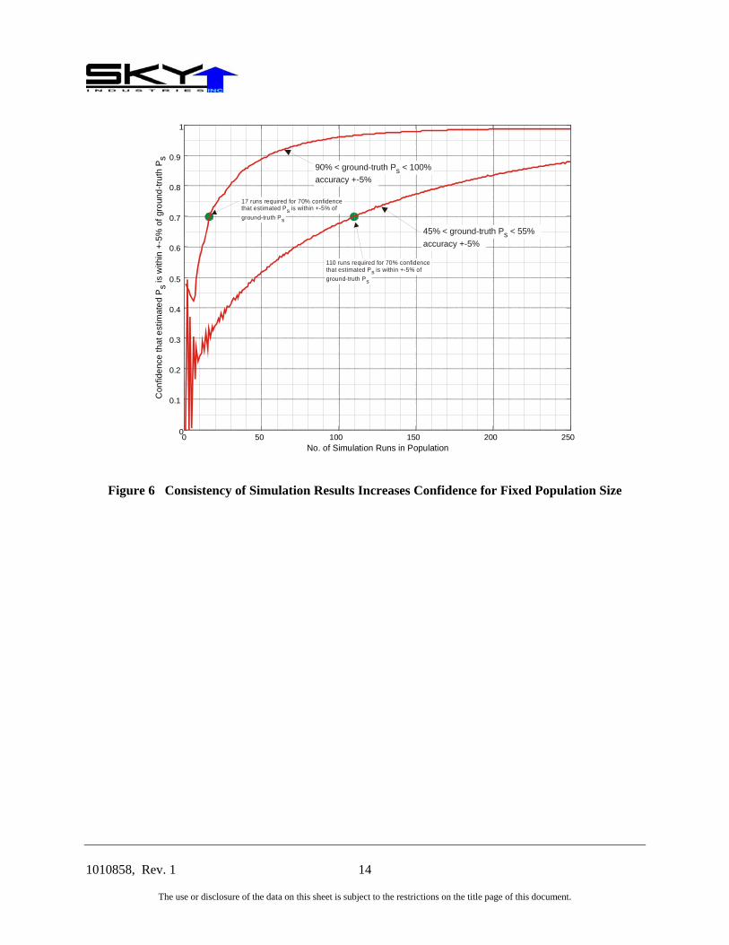
a. Consistency of simulation results increases confidence for fixed population size

If Ps is high (or low), a relatively small population size is required for a given accuracy and confidence; conversely, if a high (or low) proportion of misses are observed in a small number of simulation runs, one may conclude that the ground-truth value of Ps is high (or low) with high confidence without increasing the population size, i.e. the population size may be controlled by the evolving statistical properties of the population. An example of this effect is presented in fig. F, in which confidence curves are presented for two cases: (a) 90% < ground-truth Ps < 100% with accuracy +-5% , and (b) 45% < ground-truth Ps < 55% with accuracy +-5%. The confidence of the estimated Ps value for a given population size is higher in the former case compared with the latter, because the behaviour of individuals in the population is more consistent.

b. Consistency of simulation results decreases required population size

Referring to Figure 6, if the range of ground-truth Ps is between 90% and 100%, the estimated value of Ps will be within +-5% of the ground-truth value with 70% confidence after 17 runs. If the range is 45% to 50%, 110 runs are required to achieve the same combination of accuracy and confidence.

1010858, Rev. 1 14


0 50 100 150 200 2500

0.1

0.2

0.3

0.4

0.5

0.6

0.7

0.8

0.9

1


90% < ground-truth P < 100%accuracy +-5%

s

45% < ground-truth P < 55%accuracy +-5%

s

Con

fiden

ce th

at e

stim

ated

P is

with

in +

-5%

of g

roun

d-tru

th P

ss

17 runs required for 70% confidencethat estimated P is within +-5% of ground-truth P

ss

110 runs required for 70% confidencethat estimated P is within +-5% of ground-truth P

ss

Figure 6 Consistency of Simulation Results Increases Confidence for Fixed Population Size

1010858, Rev. 1 15


0 50 100 150 210 2500

0.1

0.2

0.3

0.4

0.5

0.6

0.7

0.8

0.9

1


Con

fiden

ce th

at e

stim

ated

P is

with

in to

lera

nce

give

n 40

% <

true

P <

80%

ss

data generated by SMCNUM.EXE and SMC1.M

+-3%

+-4%

-5%

-6%

-7%-8%

-9%-10%

-20%

+-1%

+-2%

Confidence that P is within specified tolerance after n simulation runs for ground-truth of 40% < P < 80%

ss

40302010 90807060 140130120110 190180170160 220 230 240200

100 runs in population:Estimated value of P accurate to +-2%with confidence of 32%

s

100 runs in population:Estimated value of P accurate to +-6%with confidence of 79%

s

100 runs in population:Estimated value of P accurate to +-10%with confidence of 95.5%

s

Figure 7 Illustration of Tradeoff between Accuracy and Confidence of Estimated Ps

6.2 Choosing Population Size

The steps required to choose the simulation population size for a given problem in estimating Ps are presented below.

a. Choose the desired accuracy of the estimated value of Ps

b. Choose the desired confidence that the estimated value of Ps is within the desired accuracy of the ground-truth value of Ps

c. Estimate the range of the ground-truth value of Ps

1010858, Rev. 1 16


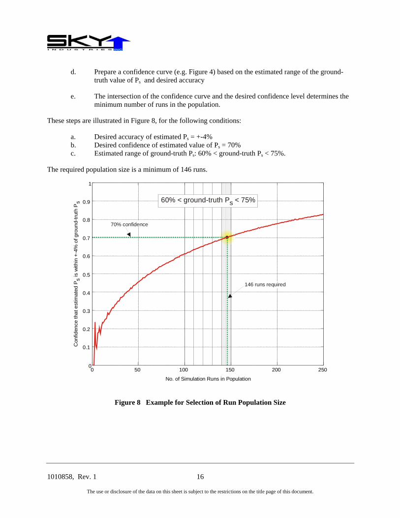
d. Prepare a confidence curve (e.g. Figure 4) based on the estimated range of the ground-truth value of Ps and desired accuracy

e. The intersection of the confidence curve and the desired confidence level determines the minimum number of runs in the population.

These steps are illustrated in Figure 8, for the following conditions:

a. Desired accuracy of estimated Ps = +-4% b. Desired confidence of estimated value of Ps = 70% c. Estimated range of ground-truth Ps: 60% < ground-truth Ps < 75%.

The required population size is a minimum of 146 runs.

0 50 100 150 200 2500

0.1

0.2

0.3

0.4

0.5

0.6

0.7

0.8

0.9

1


70% confidence

146 runs required

Con

fiden

ce th

at e

stim

ated

P is

with

in +

-4%

of g

roun

d-tru

th P

ss 60% < ground-truth P < 75%s

Figure 8 Example for Selection of Run Population Size

1010858, Rev. 1 17


6.3 Interpretation of A Priori Populations

Section 6.2 addresses the problem of choosing the population size based on accuracy and confidence requirements. The inverse of this problem involves determining admissible combinations of accuracy and confidence which apply to a data population that already exists, and whose size is therefore fixed. Such problems can arise when using data from field trials which were conducted before a particular aspect of data analysis was planned; there is no possibility of increasing the data population size.

Accuracy and confidence of estimated Ps can be traded against each other. For a given run population size, it is possible to exchange accuracy of the estimated value of Ps with confidence that the estimated value reflects the ground-truth Ps to that accuracy. As the quoted accuracy increases, the associated confidence decreases. Conversely, as the quoted accuracy decreases, the associated confidence increases. This tradeoff is illustrated in Figure 7 using the confidence curves of Figure 4, considering a population size of 100 runs.

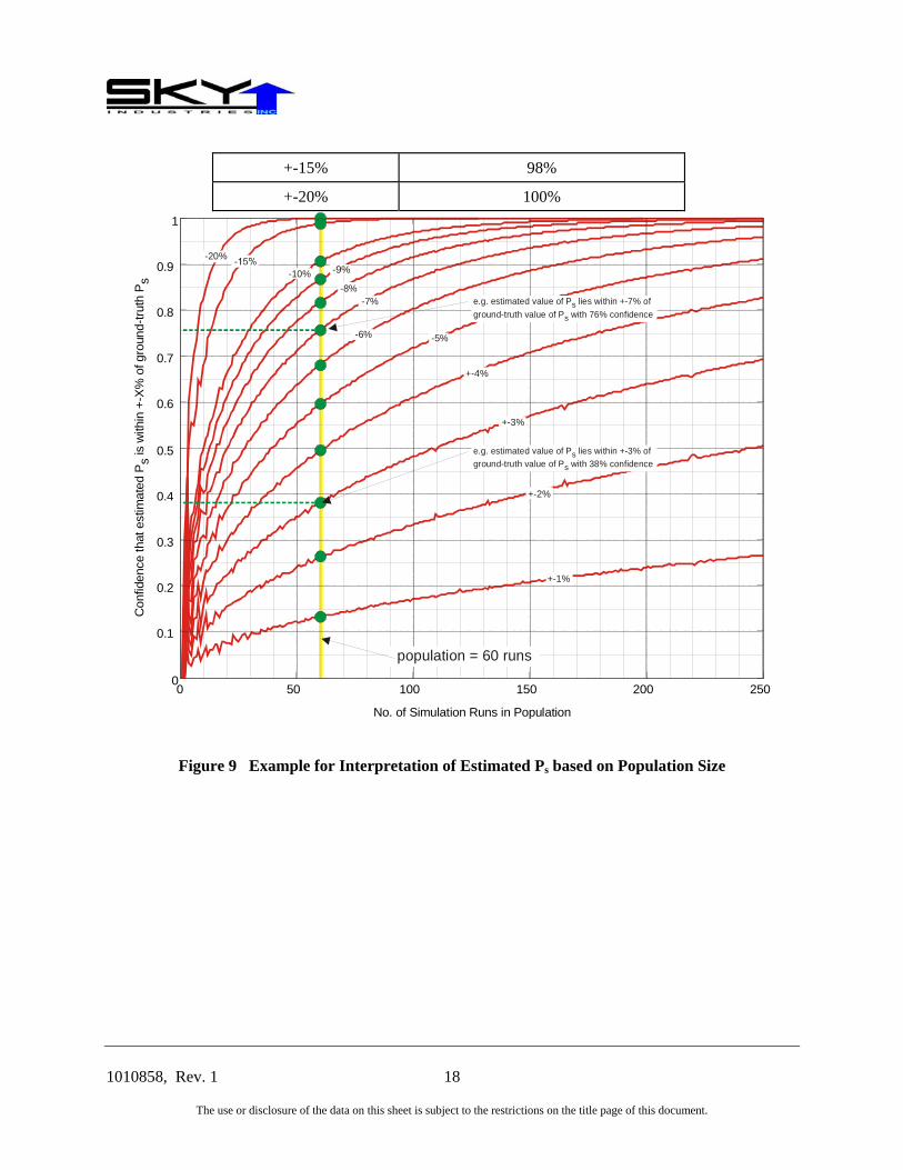
As a numerical example, consider the case of an existing population of 60 simulation runs. After suitable data analysis an estimated value of Ps is determined, which must then be interpreted in terms of accuracy and associated confidence. Admissible combinations of accuracy and confidence for the given population size can be read from a confidence graph, such as that presented in Figure 9, prepared for the case where the estimated ground-truth value of Ps is between 60% and 75%. Accuracy and confidence are independent of the estimated value of Ps; they are determined only by the expected range of the ground-truth value of Ps and the population size. Referring to Figure 9, some admissible combinations of accuracy and confidence are tabulated in Table 3.

Table 3

Accuracy of Ps estimate Confidence that estimate is within given accuracy of ground-truth value of Ps

+-1% 14%

+-2% 26%

+-3% 38%

+-4% 50%

+-5% 60%

+-6% 68%

+-7% 76%

+-8% 82%

+-9% 87%

+-10% 91%

1010858, Rev. 1 18


+-15% 98%

+-20% 100%

0 50 100 150 200 2500

0.1

0.2

0.3

0.4

0.5

0.6

0.7

0.8

0.9

1


+-3%

+-4%

-5%-6%

-7%-8%

-9%-10%

-20%

+-1%

+-2%

population = 60 runs

e.g. estimated value of P lies within +-7% of ground-truth value of P with 76% confidence

ss

e.g. estimated value of P lies within +-3% of ground-truth value of P with 38% confidence

ss

Con

fiden

ce th

at e

stim

ated

P is

with

in +

-X%

of g

roun

d-tru

th P

ss

Figure 9 Example for Interpretation of Estimated Ps based on Population Size

1010858, Rev. 1 19


7. EXTENSION TO CONTINUOUS VARIABLES

The discussion thus far has addressed populations of simulation runs in which the MOM places each member in one of two groups: hit or miss (failure or success). The analysis presented above can be extended to continuous variables by appropriately casting the MOM. Confidence curves described above can be calculated in which the members of the population are segregated according to whether the continuous variable of interest is above or below a threshold value. By repeating the analysis for two threshold values, it is possible to estimate the range of the parameter, the accuracy with which the range has been estimated, and the confidence of the accuracy.

As an example, consider the problem of estimating the Root Mean Squared (RMS) miss distance attributable to a given countermeasure used for ship defence against missile attack, and an associated confidence that the calculated RMS miss distance is accurate to +-x% of the ground-truth RMS miss distance, i.e. the RMS miss distance which would be calculated from an infinite population size. For the purposes of this analysis, the run population comprises simulated missile engagements in which the missile failed to intercept the ship, i.e. runs in which the miss distance was greater than a minimum value defining ship survival. To convert the continuous random variable to a binomial random variable, the MOM is chosen to be the condition (TRUE or FALSE) that the RMS miss distance is greater than a chosen threshold value. Confidence curves can be calculated for the assumption that y% of runs in the population will exhibit a miss distance greater than the threshold value. The confidence curves define the number of runs required for a given confidence, such that the estimated value is within a given accuracy of the ground-truth value.

The results for a numerical example are presented in Figure 10, Figure 11 and Figure 12. A population of 141 simulation runs was produced in which the minimum miss distance is 0.5 ship length from the bow or stern, where the ship length is 135 m. Confidence curves analogous to those of Figure 5 are presented in Figure 10 for accuracies of +-3%, +-4%, +-5%, +-6% and +-7%. The probability that the miss distance in the population is greater than a threshold value is presented in Figure 11, for threshold values from 0.5 ship length (67.5 m) to 20 ship lengths (2700 m). An “accuracy envelope” for the probability of observing a miss distance equal to or greater than a given threshold can be superimposed on the curve which best fits the data points. To calculate the accuracy envelope, the following steps were used:

a. Divide the probability axis into bins representing each of the ranges of ground-truth Ps curves in the curve sets of Figure 10.

b. Select a desired confidence value.

c. For each bin, the accuracy with the specified confidence corresponds to the curve in Figure 10 which crosses the specified confidence at or near 141 runs.

Because the accuracy curve is chosen from the curve sets in Figure 10 on the basis of the estimated value of Ps instead of the ground-truth value, strictly speaking the confidence is not 90% for the following reason: although the estimated value of Ps may be within +-x% of the ground-truth value, the ground-truth value may not be within +-x% of the estimated value.

The division of the probability axis into the ground-truth Ps range bins of Figure 10 is presented in Figure 11. The bins are:

1010858, Rev. 1 20


a. P(observed miss distance > threshold) = 0% to 10% (identical to 90% to 100% range) b. P(observed miss distance > threshold) = 10% to 20% (identical to 80% to 90% range) c. P(observed miss distance > threshold) = 20% to 30% (identical to 70% to 80% range) d. P(observed miss distance > threshold) = 30% to 40% (identical to 60% to 70% range) e. P(observed miss distance > threshold) = 40% to 50% (identical to 50% to 60% range).

The curves in Figure 10 which apply in each miss distance regime of Figure 11 are indicated by a bar in Figure 11, colour coded as the curves in Figure 10.

Using an arbitrarily chosen confidence value of 90%, the corresponding accuracy envelope of the probability that the miss distance in any run will exceed the threshold value as a function of miss distance threshold is shown in Figure 12. As described above, the accuracy envelope is determined from the confidence curves of Figure 10. The accuracy for 90% confidence is approximately given by the curve in each regime which crosses the 90% confidence level at a population size of 141 runs.

1010858, Rev. 1 21


(e) +-6.6% accuracy

0

0.1

0.2

0.3

0.4

0.5

0.6

0.7

0.8

0.9

1

Con

fiden

ce th

at e

stim

ated

P is

with

in +

-3%

of g

roun

d-tru

th P

ss

0 50 100 150 200 250



80% - 90%70% - 80%60% - 70%50% - 60%


(d) +-6% accuracy

0 50 100 150 200 2500

0.1

0.2

0.3

0.4

0.5


Con

fiden

ce th

at e

stim

ated

P is

with

in +

-3%

of g

roun

d-tru

th P

ss


80% - 90%70% - 80%60% - 70%50% - 60%


0.6

0.7

0.8

0.9

1

(b) +-4% accuracy

0 50 100 150 200 2500

0.1

0.2

0.3

0.4

0.5


Con

fiden

ce th

at e

stim

ated

P is

with

in +

-3%

of g

roun

d-tru

th P

ss


80% - 90%70% - 80%60% - 70%50% - 60%


0.6

0.7

0.8

0.9

1

0 50 100 150 200 2500

0.1

0.2

0.3

0.4

0.5


Con

fiden

ce th

at e

stim

ated

P is

with

in +

-3%

of g

roun

d-tru

th P

ss


80% - 90%70% - 80%60% - 70%50% - 60%


0.6

0.7

0.8

0.9

1

(c) +-5% accuracy

0

0.1

0.2

0.3

0.4

0.5

0.6

0.7

0.8

0.9

1

Con

fiden

ce th

at e

stim

ated

P is

with

in +

-3%

of g

roun

d-tru

th P

ss

(a) +-3% accuracy

0 50 100 150 200 250



80% - 90%70% - 80%60% - 70%50% - 60%


141 simulation runs

141 simulation runs

141 simulation runs

141 simulation runs

141 simulation runs

(f) +-7% accuracy

0

0.1

0.2

0.3

0.4

0.5

0.6

0.7

0.8

0.9

1

Con

fiden

ce th

at e

stim

ated

P is

with

in +

-3%

of g

roun

d-tru

th P

ss

0 50 100 150 200 250



80% - 90%70% - 80%60% - 70%50% - 60%


141 simulation runs

Figure 10 Confidence Curves for Analysis of Miss Distance Statistics

1010858, Rev. 1 22


Threshold miss distance normalized to 135 m ship length (unitless)1 2 3 4 5 6 7 8 9 10 11 12 13 14 15 16 17 18

minimum miss distance = 0.5 x ship length from bow or stern

0

Prob

abili

ty th

at m

iss

dist

ance

exc

eeds

thre

shol

d

10%

20%

30%

40%

50%

60%

70%

80%

90%

100%

0%

+-3% curve in fig. J



+-6.6% curve in fig. J+-7% curve in fig. J


+-6.6% curve in fig. J

19 20

Figure 11 Probability Range Bins for Minimum Miss Distance

1010858, Rev. 1 23


Threshold miss distance normalized to 135 m ship length (unitless)1 2 3 4 5 6 7 8 9 10 11 12 13 14 15 16 17 18 190 20

Prob

abili

ty th

at m

iss

dist

ance

exc

eeds

thre

shol

d

10%

20%

30%

40%

50%

60%

70%

80%

90%

100%

0%

Figure 12 90% Confidence Envelope for Observing Minimum Miss Distance in Run Population

1010858, Rev. 1 24


8. CONCLUSION

In conclusion, this analysis has quantitatively addressed the problem of determining the required size of a population of statistically independent trials, when estimating a property of the population which represents a binomial random variable. i.e. analogous to a coin toss problem.

The size of the population has been related to the accuracy with which the estimated value lies within the ground-truth value, and the confidence that the quoted accuracy applies. For a given problem, confidence curves can be calculated based on binomial probability density functions, and these curves related population size, accuracy of the estimated parameter, and the associated confidence of the accuracy of the estimate.

This analysis can be extended from binomial random variables to continuous random variables.

UNCLASSIFIED SECURITY CLASSIFICATION OF FORM

(highest classification of Title, Abstract, Keywords)

DOCUMENT CONTROL DATA (Security classification of title, body of abstract and indexing annotation must be entered when the overall document is classified)

1. ORIGINATOR (the name and address of the organization preparing the document. Organizations for whom the document was prepared, e.g. Establishment sponsoring a contractor’s report, or tasking agency, are entered in section 8.)

Sky Industries Inc. 2956 McCarthy Rd Ottawa ON Canada K1V 8K6

2. SECURITY CLASSIFICATION (overall security classification of the document,

including special warning terms if applicable) UNCLASSIFIED

3. TITLE (the complete document title as indicated on the title page. Its classification should be indicated by the appropriate abbreviation (S,C or U) in parentheses after the title.)

Calculation of Required Population Size for Desired Confidence and Accuracy of Results

4. AUTHORS (Last name, first name, middle initial)

Charland, Shawn

5. DATE OF PUBLICATION (month and year of publication of document)

April 2004

6a. NO. OF PAGES (total containing information. Include Annexes, Appendices, etc.)

28

6b. NO. OF REFS (total cited in document)

1

7. DESCRIPTIVE NOTES (the category of the document, e.g. technical report, technical note or memorandum. If appropriate, enter the type of report, e.g. interim, progress, summary, annual or final. Give the inclusive dates when a specific reporting period is covered.)

CCoonnttrraacctt rreeppoorrtt

8. SPONSORING ACTIVITY (the name of the department project office or laboratory sponsoring the research and development. Include the address.) DRDC Ottawa 3701 Carling Ave Ottawa Ontario, K1A 0Z4, Canada

9a. PROJECT OR GRANT NO. (if appropriate, the applicable research and development project or grant number under which the document was written. Please specify whether project or grant)

SISWS

9b. CONTRACT NO. (if appropriate, the applicable number under which the document was written)

W7714-030726

10a. ORIGINATOR’S DOCUMENT NUMBER (the official document number by which the document is identified by the originating activity. This number must be unique to this document.)

DRDC Ottawa CR 2004-001

10b. OTHER DOCUMENT NOS. (Any other numbers which may be assigned this document either by the originator or by the sponsor)

11. DOCUMENT AVAILABILITY (any limitations on further dissemination of the document, other than those imposed by security classification) ( X ) Unlimited distribution ( ) Distribution limited to defence departments and defence contractors; further distribution only as approved ( ) Distribution limited to defence departments and Canadian defence contractors; further distribution only as approved ( ) Distribution limited to government departments and agencies; further distribution only as approved ( ) Distribution limited to defence departments; further distribution only as approved ( ) Other (please specify):

12. DOCUMENT ANNOUNCEMENT (any limitation to the bibliographic announcement of this document. This will normally correspond to the Document Availability (11). However, where further distribution (beyond the audience specified in 11) is possible, a wider announcement audience may be selected.)

UNCLASSIFIED

SECURITY CLASSIFICATION OF FORM DDCCDD0033 22//0066//8877


13. ABSTRACT ( a brief and factual summary of the document. It may also appear elsewhere in the body of the document itself. It is highly desirable that the abstract of classified documents be unclassified. Each paragraph of the abstract shall begin with an indication of the security classification of the information in the paragraph (unless the document itself is unclassified) represented as (S), (C), or (U). It is not necessary to include here abstracts in both official languages unless the text is bilingual).

The purpose of this report is to describe a quantitative mathematical foundation for the following:

a. Calculate the required number of simulation runs or trials in order to determine the ECM effectiveness to a desired accuracy and confidence

b. Determine the accuracy of the ECM effectiveness as calculated from a population of simulation runs or trials, based on the run population size

c. Determine the confidence level of the ECM effectiveness, based on the run population size.

AAlltthhoouugghh tthhee aannaallyyssiiss pprreesseenntteedd hheerree aapppplliieess eeqquuaallllyy ttoo ssooffttwwaarree ssiimmuullaattiioonn aanndd hhaarrddwwaarree ttrriiaallss,, tthhee tteerrmm ““ssiimmuullaattiioonn rruunnss”” sshhaallll bbee uusseedd ttoo rreeffeerr eeqquuaallllyy ttoo ssooffttwwaarree ssiimmuullaattiioonn aanndd hhaarrddwwaarree ttrriiaallss..

14. KEYWORDS, DESCRIPTORS or IDENTIFIERS (technically meaningful terms or short phrases that characterize a document and could be helpful in cataloguing the document. They should be selected so that no security classification is required. Identifiers such as equipment model designation, trade name, military project code name, geographic location may also be included. If possible keywords should be selected from a published thesaurus. e.g. Thesaurus of Engineering and Scientific Terms (TEST) and that thesaurus-identified. If it is not possible to select indexing terms which are Unclassified, the classification of each should be indicated as with the title.)

ECM effectiveness Probability of soft-kill Accuracy Confidence level Monte Carlo Simulation Trials


Shipboard Integrated Sensors and Weapons Systems...

Documents

Transcript of Shipboard Integrated Sensors and Weapons Systems...