Ship Response Capability Models for Counter-Piracy Patrols ...

Défense

nationale

National

Defence

Defence R&D CanadaCentre for Operational Research and Analysis

Maritime ORT

DRDC CORA TM 2011-139September 2011

Ship Response Capability Modelsfor Counter-Piracy Patrols in theGulf of Aden

Ramzi MirshakMaritime Operational Research Team

Ship Response Capability Models forCounter-Piracy Patrols in the Gulf of Aden

Ramzi MirshakMaritime Operational Research Team

Defence R&D Canada – CORATechnical MemorandumDRDC CORA TM 2011-139September 2011

Principal Author

Original signed by Dr. R. Mirshak

Dr. R. Mirshak

Approved by

Original signed by Dr. R.E. Mitchell

Dr. R.E. Mitchell

Head Maritime and ISR Operational Research

Approved for release by

Original signed by P. Comeau

P. Comeau

Chief Scientist

The information contained herein has been derived and determined through best practice

and adherence to the highest levels of ethical, scientific and engineering investigative prin-

ciples. The reported results, their interpretation, and any opinions expressed therein, re-

main those of the authors and do not represent, or otherwise reflect, any official opinion or

position of DND or the Government of Canada.

c© Her Majesty the Queen in Right of Canada as represented by the Minister of National

Defence, 2011

c© Sa Majesté la Reine (en droit du Canada), telle que représentée par le ministre de la

Défense nationale, 2011

Abstract

This work examines the capability-models of ships performing counter-piracy patrols in the

International Recommended Transit Corridor, located in Gulf of Aden (GOA). Specifically,

it considers possible approaches to predict the response time of assets patrolling long and

thin regions and to facilitate coordination between multiple assets.

For situations where the pirate attacks occur randomly, the across-channel location of the

ship prior to the attack has only a limited impact on the response-time probability distri-

bution, supporting the notion that the problem can be examined in a one-dimensional (1D)

context. It is demonstrated that the 1D approach is extremely effective at reproducing the

cumulative distributions of higher fidelity models. The 1D approach is then used to demon-

strate that coordinating patrol ship positions is a key factor, while coordinating the rotation

of helicopter crews between ships may be less important. It is also shown that for the types

of wind fields in which pirates will operate in the GOA, a ship can reposition itself in a

manner such that the winds will not heavily affect response capabilities.

Finally, a description of how the results from this work can be applied in the development of

an asset positioning model are presented, and a description of the way forward is provided.

Résumé

Ce travail porte sur les modèles de capacité des navires qui effectuent des patrouilles de

lutte contre la piraterie dans le couloir de transit international recommandé (IRTC), situé

dans le golfe d’Aden. Plus précisément, il examine les façons possibles de prévoir le dé-

lai d’intervention des ressources qui patrouillent dans des régions longues et étroites et de

faciliter la coordination entre de multiples ressources. Dans les cas où les attaques de pi-

rates ont lieu au hasard, l’emplacement du navire de l’autre côté du chenal avant l’attaque

n’a qu’une incidence limitée sur la distribution probabiliste du délai d’intervention, ce qui

corrobore l’idée selon laquelle le problème peut être examiné dans un contexte unidimen-

sionnel (1D). Il est démontré que l’approche 1D est extrêmement efficace pour reproduire

les distributions cumulatives de modèles de plus grande fidélité. Cette approche est ensuite

utilisée pour démontrer que la coordination des positions des navires de patrouille consti-

tue un facteur clé, tandis que la coordination de la rotation des équipages d’hélicoptère

entre les navires peut s’avérer moins importante. Il est également établi que pour les types

de champs de vent dans lesquels les pirates opéreront dans le golfe d’Aden, un navire

peut se repositionner de manière à ce que les vents ne nuisent pas beaucoup aux capacités

d’intervention. Enfin, le document renferme une description de la façon dont les résultats

de ce travail peuvent être appliqués à l’élaboration d’un modèle de positionnement des

ressources, ainsi qu’une description de la voie à suivre.

DRDC CORA TM 2011-139 i

This page intentionally left blank.

ii DRDC CORA TM 2011-139

Executive summary

Ship Response Capability Models for Counter-PiracyPatrols in the Gulf of Aden

Ramzi Mirshak; DRDC CORA TM 2011-139; Defence R&D Canada – CORA;September 2011.

Background: The Gulf of Aden is an approximately 450 nm-long section of water con-

necting the Gulf of Oman to the Arabian Sea, and is bordered by Yemen to the north and

Somalia to the south. It is a major commercial shipping corridor, with 12% of the world’s

daily oil supply traveling through the region. In recent years, Somali-based piracy has

flourished, posing a threat to international trade and freedom of the seas. In 2007, the In-

ternational Maritime Bureau (IMB) reported 43 incidents of piracy around near Somalia,

increasing to 111 in 2008. By the end of September 2009, over 300 events had taken place

in that year so far. To help control piracy in the area, coalition forces responded to the area.

To improve the effectiveness of patrol coverage, the 12 nm-wide International Recom-

mended Transit Corridor (IRTC) was introduced, with the purpose of focusing traffic into

an easier to manage and better defined region. However, few planning tools are presently

available to assist analysts and planners when it comes to allocating ships to patrol this

region in an optimal fashion.

Principal Results: The work presented here identifies the probability that an arbitrary ship

can respond to an act of piracy at some random location within its area of responsibility,

or patrol area. Four patrol strategies are presented for a two-dimensional (2D) model and

a one-dimensional (1D) simplification of that model. Both the 2D and 1D models can

produce the probability of a ship responding to an incident of piracy in a specific time

frame, using the ship profile, the size of the patrol region, and the patrol strategy as inputs.

The 1D model is computationally simpler than its 2D counterpart, however, which makes

it more amenable for considering more complex multiple-ship problems.

It is shown that ships that remain at the centre of their patrol region will consistently out-

perform those that travel along its length, and that the effects of moving across its (narrow)

width can be accounted for while essentially restricting the problem to a 1D-nature. Simple

two-ship and three-ship problems are presented to examine how ships with various patrol

strategies (representing various degrees of cooperation with coalition command) can be

coordinated. It is shown that coordinated efforts that optimize the spacing between ships

will consistently out-perform uncoordinated efforts. A simple model also demonstrates

that a ship can position itself within a patrol area to accommodate the effects of wind on

helicopter range in a manner that permits wind to be neglected in initial calculation of ship

positions. These findings lead to the following recommendations:

DRDC CORA TM 2011-139 iii

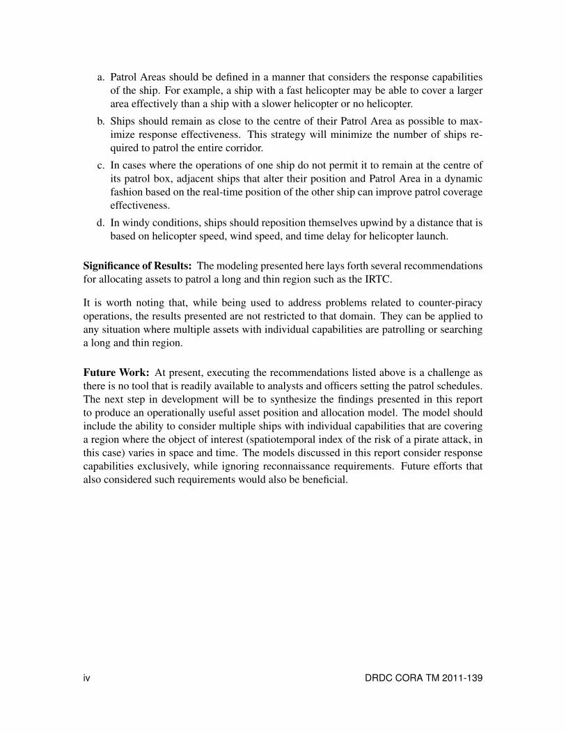
a. Patrol Areas should be defined in a manner that considers the response capabilities

of the ship. For example, a ship with a fast helicopter may be able to cover a larger

area effectively than a ship with a slower helicopter or no helicopter.

b. Ships should remain as close to the centre of their Patrol Area as possible to max-

imize response effectiveness. This strategy will minimize the number of ships re-

quired to patrol the entire corridor.

c. In cases where the operations of one ship do not permit it to remain at the centre of

its patrol box, adjacent ships that alter their position and Patrol Area in a dynamic

fashion based on the real-time position of the other ship can improve patrol coverage

effectiveness.

d. In windy conditions, ships should reposition themselves upwind by a distance that is

based on helicopter speed, wind speed, and time delay for helicopter launch.

Significance of Results: The modeling presented here lays forth several recommendations

for allocating assets to patrol a long and thin region such as the IRTC.

It is worth noting that, while being used to address problems related to counter-piracy

operations, the results presented are not restricted to that domain. They can be applied to

any situation where multiple assets with individual capabilities are patrolling or searching

a long and thin region.

Future Work: At present, executing the recommendations listed above is a challenge as

there is no tool that is readily available to analysts and officers setting the patrol schedules.

The next step in development will be to synthesize the findings presented in this report

to produce an operationally useful asset position and allocation model. The model should

include the ability to consider multiple ships with individual capabilities that are covering

a region where the object of interest (spatiotemporal index of the risk of a pirate attack, in

this case) varies in space and time. The models discussed in this report consider response

capabilities exclusively, while ignoring reconnaissance requirements. Future efforts that

also considered such requirements would also be beneficial.

iv DRDC CORA TM 2011-139

Sommaire

Ship Response Capability Models for Counter-PiracyPatrols in the Gulf of Aden

Ramzi Mirshak ; DRDC CORA TM 2011-139 ; R & D pour la défense Canada –CARO ; septembre 2011.

Contexte : Le golfe d’Aden est une étendue d’eau d’environ 450 NM de longueur qui

relie le golfe d’Oman à la mer d’Arabie et qui est bordée au nord par le Yémen et au

sud par la Somalie. Il s’agit d’un important couloir de navigation commerciale, et 12%

des approvisionnements mondiaux en pétrole passent par cette région tous les jours. Ces

dernières années, les actes commis par des pirates basés en Somalie se sont multipliés,

posant ainsi une menace pour le commerce international et la liberté des mers. En 2007, le

Bureau maritime international (BMI) a signalé 43 incidents de piraterie près de la Somalie,

et ce nombre est passé à 111 en 2008. À la fin de septembre 2009, plus de 300 incidents

avaient eu lieu cette année-là. Des forces coalisées sont intervenues pour aider à enrayer

la piraterie dans la région. Afin d’accroître l’efficacité de la couverture du patrouille, on

a créé le couloir de transit international recommandé (IRTC), d’une largeur de 12 NM,

en vue de concentrer la circulation dans une région mieux définie et plus facile à gérer.

Toutefois, il existe actuellement peu d’outils de planification pour aider les analystes et les

planificateurs lorsqu’il s’agit d’affecter des navires pour patrouiller dans cette région de

manière optimale.

Résultats principaux : Le présent document indique la probabilité qu’un navire arbitraire

puisse réagir à un acte de piraterie commis quelque part au hasard dans son secteur de res-

ponsabilité ou de patrouille. Quatre stratégies de patrouille sont présentées à l’égard d’un

modèle bidimensionnel (2D) et d’une simplification unidimensionnelle (1D) de ce modèle.

En utilisant comme intrants le profil du navire, la superficie de la région de patrouille et

la stratégie de patrouille, les modèles 2D et 1D peuvent tous deux produire la probabilité

qu’un navire réagisse à un incident de piraterie dans un délai précis. Le modèle 1D est

cependant plus simple que le modèle 2D sur le plan du calcul, ce qui facilite son utilisation

dans le cas de problèmes plus complexes mettant en cause plusieurs navires. Il est démontré

que les navires qui restent au centre de leur région de patrouille auront toujours de meilleurs

résultats que ceux qui se déplacent le long du bord du secteur, et que les effets de la traver-

sée du chenal (étroit) peuvent être justifiés tout en limitant essentiellement le problème à

un contexte unidimensionnel. Des problèmes simples à deux navires et à trois navires sont

présentés afin d’examiner comment l’on peut coordonner des navires ayant diverses stra-

tégies de patrouille (qui représentent divers degrés de coopération avec le commandement

de la coalition). Il est établi que des efforts coordonnés qui optimisent l’espacement entre

DRDC CORA TM 2011-139 v

les navires donneront toujours de meilleurs résultats que des efforts non coordonnés. Un

modèle simple démontre également qu’un navire peut se positionner dans un secteur de pa-

trouille afin de tenir compte des effets du vent sur le rayon d’action de l’hélicoptère, ce qui

permet de négliger le vent dans le calcul initial de la position des navires. Ces constatations

donnent lieu aux recommandations suivantes :

a. Il faudrait définir les secteurs de patrouille de façon à prendre en considération les

capacités d’intervention du navire. Par exemple, un navire doté d’un hélicoptère ra-

pide peut être capable de couvrir efficacement un secteur plus vaste qu’un navire

dont l’hélicoptère est moins rapide ou qui ne possède pas d’hélicoptère.

b. Les navires devraient rester le plus près possible du centre de leur secteur de pa-

trouille afin de maximiser l’efficacité de l’intervention. Cette stratégie réduira au

minimum le nombre de navires qui doivent patrouiller dans tout le couloir.

c. Dans les cas oû les opérations d’un navire ne lui permettent pas de rester au centre de

sa zone de patrouille, l’efficacité de la couverture peut être améliorée si des navires

adjacents modifient leur position et leur secteur de patrouille de façon dynamique en

fonction de la position en temps réel de l’autre navire.

d. Par temps venteux, les navires devraient se repositionner au vent selon une distance

fondée sur la vitesse de l’hélicoptère, la vitesse du vent et le délai de décollage de

l’hélicoptère.

Portée des résultats : La modélisation présentée ici permet de formuler plusieurs recom-

mandations concernant l’affectation des ressources nécessaires pour patrouiller dans une

région longue et étroite comme l’IRTC. Il convient de noter que, même s’ils servent à

traiter des problèmes liés aux opérations de lutte contre la piraterie, les résultats présen-

tés ne sont pas limités à ce domaine. En effet, ils peuvent être appliqués à toute situation

oû de multiples ressources aux capacités individuelles effectuent des patrouilles ou des

recherches dans une région longue et étroite.

Recherches futures : À l’heure actuelle, la mise en œuvre des recommandations susmen-

tionnées pose des difficultés, car aucun outil n’est mis à la disposition des analystes et des

officiers qui établissent les calendriers de patrouille. La prochaine étape dans le dévelop-

pement consistera à faire la synthèse des constatations formulées dans le présent rapport

afin de produire un modèle d’affectation et de positionnement des ressources qui soit utile

sur le plan opérationnel. Ce modèle devrait inclure la capacité de considérer plusieurs na-

vires aux capacités individuelles qui couvrent une région oû l’objet d’intérêt (dans le cas

présent, l’indice spatio-temporel du risque d’attaque de pirates) varie dans l’espace et dans

le temps. Les modèles dont il est question dans ce rapport considèrent exclusivement les

capacités d’intervention, sans tenir compte des exigences en matière de reconnaissance. Il

serait également avantageux de consacrer de futurs travaux à l’étude de ces exigences.

vi DRDC CORA TM 2011-139

Table of contents

Abstract . . . . . . . . . . . . . . . . . . . . . . . . . . . . . . . . . . . . . . . . . i

Résumé . . . . . . . . . . . . . . . . . . . . . . . . . . . . . . . . . . . . . . . . . i

Executive summary . . . . . . . . . . . . . . . . . . . . . . . . . . . . . . . . . . . iii

Sommaire . . . . . . . . . . . . . . . . . . . . . . . . . . . . . . . . . . . . . . . . v

Table of contents . . . . . . . . . . . . . . . . . . . . . . . . . . . . . . . . . . . . vii

List of figures . . . . . . . . . . . . . . . . . . . . . . . . . . . . . . . . . . . . . . x

List of tables . . . . . . . . . . . . . . . . . . . . . . . . . . . . . . . . . . . . . . . xi

1 Introduction . . . . . . . . . . . . . . . . . . . . . . . . . . . . . . . . . . . . . 1

1.1 Background: Shipping, Piracy and Counter-Piracy in the Gulf of Aden . . 3

1.2 Scope of Work . . . . . . . . . . . . . . . . . . . . . . . . . . . . . . . . 5

2 Ship Response Models . . . . . . . . . . . . . . . . . . . . . . . . . . . . . . . 8

2.1 2D Patrol Coverage Models . . . . . . . . . . . . . . . . . . . . . . . . . 8

2.1.1 Monte Carlo Approach . . . . . . . . . . . . . . . . . . . . . . . 9

2.1.2 Ripple Propagation Algorithm . . . . . . . . . . . . . . . . . . . 9

2.1.3 Marsaglia et al. Algorithm . . . . . . . . . . . . . . . . . . . . . 9

2.1.4 Comparison of 2D Algorithms . . . . . . . . . . . . . . . . . . . 11

2.2 1D Patrol Coverage Model . . . . . . . . . . . . . . . . . . . . . . . . . . 11

2.2.1 Why a 1D Model? . . . . . . . . . . . . . . . . . . . . . . . . . 11

2.2.2 Model Description . . . . . . . . . . . . . . . . . . . . . . . . . 13

2.2.3 Calculating Patrol Coverage . . . . . . . . . . . . . . . . . . . . 14

2.2.4 Error Correction . . . . . . . . . . . . . . . . . . . . . . . . . . 14

2.2.5 Limitations . . . . . . . . . . . . . . . . . . . . . . . . . . . . . 17

DRDC CORA TM 2011-139 vii

3 Patrol and Positioning Strategies . . . . . . . . . . . . . . . . . . . . . . . . . . 18

3.1 Comparison of Patrol Strategies for the One-Ship Problem . . . . . . . . . 18

3.2 Identifying the likelihood of a 30-minute response time . . . . . . . . . . 21

3.3 Coordinating Multiple TF Assets . . . . . . . . . . . . . . . . . . . . . . 21

3.3.1 Assigning Patrol Boxes to Optimize Response . . . . . . . . . . . 21

3.3.2 Considering Helicopter Readiness . . . . . . . . . . . . . . . . . 25

3.4 Altering Ship Position to Compensate for Wind . . . . . . . . . . . . . . . 28

4 Findings, Recommendations and Future Work . . . . . . . . . . . . . . . . . . . 31

4.1 Findings . . . . . . . . . . . . . . . . . . . . . . . . . . . . . . . . . . . 31

4.2 Recommendations . . . . . . . . . . . . . . . . . . . . . . . . . . . . . . 31

4.3 Future Work: Proposed Allocation Model . . . . . . . . . . . . . . . . . . 32

References . . . . . . . . . . . . . . . . . . . . . . . . . . . . . . . . . . . . . . . . 34

Annex A: Response-Time Uncertainties . . . . . . . . . . . . . . . . . . . . . . . 35

A.1 Time Required to Cover a Known Distance . . . . . . . . . . . . 35

A.2 Distance Covered in a Known Time . . . . . . . . . . . . . . . . 36

A.3 Covering a Known Distance in a Known Time . . . . . . . . . . . 39

A.4 Application to 2D models . . . . . . . . . . . . . . . . . . . . . . 39

A.5 Application to 1D Model . . . . . . . . . . . . . . . . . . . . . . 42

A.6 Other Time Delays . . . . . . . . . . . . . . . . . . . . . . . . . 42

Annex B: Radial Propagation Algorithm . . . . . . . . . . . . . . . . . . . . . . . 43

B.1 Calculation of PDF . . . . . . . . . . . . . . . . . . . . . . . . . 43

B.2 Application to Patrol Strategies . . . . . . . . . . . . . . . . . . . 44

B.2.1 Centred . . . . . . . . . . . . . . . . . . . . . . . . . . . 45

B.2.2 Random Along . . . . . . . . . . . . . . . . . . . . . . . 45

viii DRDC CORA TM 2011-139

B.2.3 Random Across . . . . . . . . . . . . . . . . . . . . . . 45

B.2.4 Random . . . . . . . . . . . . . . . . . . . . . . . . . . 45

Annex C: Theory of Marsaglia et al. (1990) . . . . . . . . . . . . . . . . . . . . . 47

Annex D: Error Calculations for 1D model . . . . . . . . . . . . . . . . . . . . . . 51

D.1 Stationary Mode: Asset Remains Centred Between Shipping Lanes 51

D.2 Across Mode: Asset Travels Across Shipping Lanes . . . . . . . . 53

D.3 Range Coverage . . . . . . . . . . . . . . . . . . . . . . . . . . . 54

List of Abbreviations Used . . . . . . . . . . . . . . . . . . . . . . . . . . . . . . . 56

List of Mathematical Symbols Used . . . . . . . . . . . . . . . . . . . . . . . . . . 57

DRDC CORA TM 2011-139 ix

List of figures

Figure 1: Screenshot of GAPP version 2.2. . . . . . . . . . . . . . . . . . . . . . 2

Figure 2: Map of Gulf of Aden (GOA) with International Recommended Transit

Corridor (IRTC). . . . . . . . . . . . . . . . . . . . . . . . . . . . . . 4

Figure 3: Depiction of TF Patrol Strategies . . . . . . . . . . . . . . . . . . . . . 6

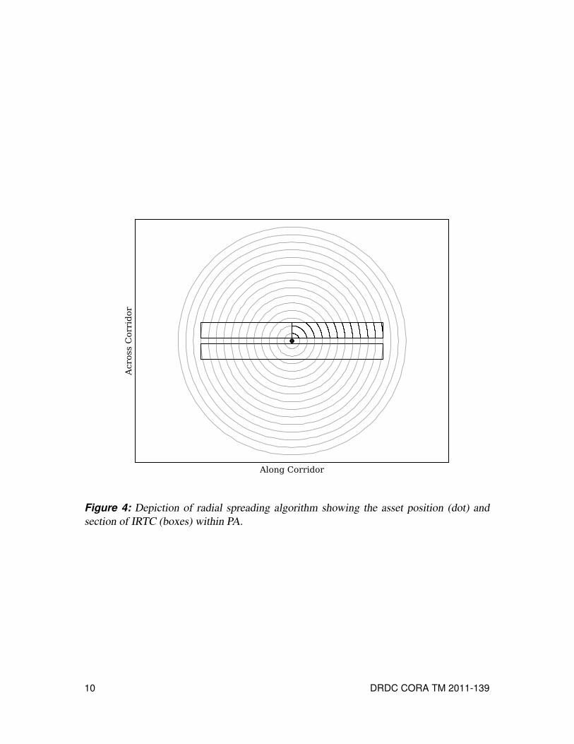
Figure 4: Depiction of radial spreading algorithm showing the asset position

(dot) and section of IRTC (boxes) within PA. . . . . . . . . . . . . . . . 10

Figure 5: Comparison of Monte Carlo and 2D Theoretical models. . . . . . . . . 12

Figure 6: Limitation of GAPP when dealing with multiple-asset response

capabilities. . . . . . . . . . . . . . . . . . . . . . . . . . . . . . . . . 12

Figure 7: Decomposition of 2D space into 1D patrol strategies (Random-1D and

Centred-1D) and corrections (Across and Stationary). . . . . . . . . . . 13

Figure 8: Geometry used to identify overestimation of area covered by 1D model. 15

Figure 9: Average area overestimation factor by 1D model. . . . . . . . . . . . . 16

Figure 10: PDFs of range to target for four Patrol Strategies in a 60 nm-long PA. . . 19

Figure 11: PDFs of distance (fill) and times (lines) separating TF ship from site of

pirate attack for the three ships profiles given in Table 1. . . . . . . . . . 20

Figure 12: Model comparison of response capabilities for Ship A, given a

30-minute response window. . . . . . . . . . . . . . . . . . . . . . . . 22

Figure 13: Model comparison of response capabilities for Ship A without a

helicopter, given a 30-minute response window. . . . . . . . . . . . . . 23

Figure 14: Dynamic positioning of Ship A based on location of Ship B. . . . . . . 24

Figure 15: Response capabilities for a two-ship problem. . . . . . . . . . . . . . . 25

Figure 16: Effect of helicopter readiness on response capabilities. . . . . . . . . . . 27

Figure 17: Compensation of ship location to account for wind. . . . . . . . . . . . 29

Figure 18: Distance upwind that a ship position should be shifted to cover patrol

region. . . . . . . . . . . . . . . . . . . . . . . . . . . . . . . . . . . . 30

x DRDC CORA TM 2011-139

Figure A.1: Average transit speed for a helicopter with normally distributed launch

delay (top panel), and representative response times (bottom panels). . . 37

Figure A.2: Velocity profiles for 2D model using exact and probabilistic treatments

to helicopter launch time. . . . . . . . . . . . . . . . . . . . . . . . . . 38

Figure A.3: 30-minute range of various assets. . . . . . . . . . . . . . . . . . . . . 40

Figure A.4: Deriving PDF of response times from PDF of response distance with

uncertainty in helicopter launch. . . . . . . . . . . . . . . . . . . . . . 41

Figure B.1: (Left) Division of Patrol Area based on asset position. (Right)

Dimensions used in calculations. . . . . . . . . . . . . . . . . . . . . . 44

Figure C.1: Spatial parameters used to describe rectangles. . . . . . . . . . . . . . . 48

Figure D.1: Area calculations used to determine overestimation correction for 1D

model. . . . . . . . . . . . . . . . . . . . . . . . . . . . . . . . . . . . 52

Figure D.2: Calculating error correction when ship travels remains centred in

corridor. . . . . . . . . . . . . . . . . . . . . . . . . . . . . . . . . . . 53

Figure D.3: Calculating error correction when ship travels across corridor. . . . . . . 55

List of tables

Table 1: Profile of generic ships used in modeling efforts. . . . . . . . . . . . . . 7

Table 2: Linkage between 2D and 1D patrol coverage models . . . . . . . . . . . 16

Table 3: Statistics for optimal patrol box sizes for Ships A and B covering a

150 nm section of the IRTC. . . . . . . . . . . . . . . . . . . . . . . . 26

DRDC CORA TM 2011-139 xi


xii DRDC CORA TM 2011-139

1 Introduction

1. In 2009, the Maritime Systems Group (MAR) of The Technical Cooperation Program

(TTCP) granted a 1-year extension to Action Group 10 of MAR (TTCP MAR AG-10),

expanding its mandate to consider counter-piracy (CP) operations. Motivation for the ex-

tension was based on the increasing pirate activity in the Gulf of Aden (GOA) and Somali

Basin. In a given year, over 20,000 commercial vessels transit the waters targeted by pi-

rates off Somalia, with captured ships often fetching ransoms of several million US dollars

as the endangered crews are held hostage.

2. To counter the problem, the international naval community has put forth considerable

effort to reduce and control maritime piracy in the region. This effort has included the

creation of several international coalitions or task forces (TFs). These TFs work together in

scheduling patrols and allocating assets 1 in a coordinated effort. However, there are other

vessels performing counter-piracy operations that are not a part of any coalition and may

not cooperate closely with them. This provides a challenge of allocating assets in a manner

that minimizes the duplication of effort between taskings from the above-mentioned task

forces, and the less coordinated ships of other nations.

3. One tool provided to planners at Combined Maritime Forces Headquarters (CMF HQ)

was the GOA Anti-Piracy Planning Tool (GAPP, see Figure 1) [1]. In its earlier versions,

GAPP used sets of Monte Carlo simulations to determine the time required for a ship with a

helicopter to respond to an act of piracy within a rectangular patrol area like those assigned

to ships in the GOA. In its most recent iteration, GAPP treats the problem analytically [2].

The tool illustrates how ship speed, helicopter speed, and helicopter launch delay affect

likely response times for a single ship. A primary reason for developing this tool was that

CMF HQ set the objective of TF ships patrolling shipping lanes within the GOA to be able

to respond to pirate incidents within 30 minutes of a merchant vessel broadcasting that it

was under attack [3]. Existing estimates did not include probabilistic effects, something

that GAPP provides. However, GAPP is a simple and limited tool that is not amenable to

examining the use of multiple ships to collectively cover a region of interest.

4. This report presents analyses that follow-up on those provided by GAPP, discussing

how patrol strategies in the GOA can be managed to improve the probability of responding

to a pirate attack within a specified time frame. It presents several probability modeling

approaches that can be used to measure response capabilities, then uses the models to

examine the likelihood that assets with various capabilities and patrol strategies, working

either together or independently, will respond to events within a particular time period. It

also discusses the way forward for developing a multi-ship asset allocation tool, part of the

ongoing development under the auspices of TTCP MAR AG-14.

1. The term “asset” or “Task Force asset” describes a naval ship that may or may not have a helicopter.

DRDC CORA TM 2011-139 1

Figu

re1:

Scr

eensh

ot

of

GA

PP

ver

sion

2.2

.

2 DRDC CORA TM 2011-139

1.1 Background: Shipping, Piracy and Counter-Piracyin the Gulf of Aden

5. Bordered by Yemen to the north and Somalia to the south, the GOA is an approx-

imately 450 nm-long body of water that connects the Gulf of Oman to the Arabian Sea

(Figure 2). It is a major commercial corridor for ships wishing to use the Suez Canal

to travel from the Indian Ocean to the Mediterranean Sea (or vice-versa). Estimates of the

number of ships transiting the GOA are as high as 20,000 per year, with the cargo including

12% of the world’s daily oil supply [4]. In addition to providing a challenge for commer-

cial shipping and international trade, the acts of piracy in the GOA threaten the delivery

of humanitarian aid and ransom payments are thought to be financing regional conflict and

possibly terrorism [5].

6. Somali-based piracy has flourished in recent years. In 2007, the International Mar-

itime Bureau (IMB) reported 43 incidents of piracy in the waters near Somalia, increasing

to 111 in 2008 [6]. By the end of September 2009, over 300 events had taken place in that

year [7]. Industry has put forth considerable effort to mitigate the piracy problems. Some

larger companies such as Maersk have altered some shipping routes, choosing to avoid the

GOA and take the long route around Africa (at a cost of up to $1 Million per transit) [4]. In

addition, the IMB has consulted with major international commercial partners to develop a

Best Management Practices guide [8] to give ship Masters advice and information on how

to avoid being pirated.

7. Military partners have also put forth considerable effort, creating several joint task

forces with counter-piracy mandates. The North Atlantic Treaty Organization (NATO) has

commissioned several operations, the European Union (EU) created EU NAVFOR, and

the Combined Maritime Forces (CMF) created Combined Task Force (CTF) 151. These

commands work in a coordinated way to manage counter-piracy operations off Somalia,

but other navies not affiliated with these groups also deploy ships to the region.

8. Findings from operational analysts deployed to CMF headquarters have demonstrated

that if naval forces are able to arrive on the scene of an attempted act of piracy before the

pirates have been able to board the ship, then the pirates will abort their attack and attempt

to dispose of any weapons or other pirate-related paraphernalia before they are captured

[3]. This practice makes the objective of deterring pirates a question of arriving on scene

as quickly as possible, rather than necessarily capturing suspected pirates. Experience

suggests that when a commercial vessel comes under attack by pirates and sends out a call

for assistance, naval forces have at most thirty minutes to respond [3], although it may be

considerably less. The naval response usually involves a ship transiting towards the site of

an attack and launching its helicopter (if available) to interdict more quickly.

9. The GOA is a vast region, making it difficult to perform effective CP patrols over

its entirety. To make patrols more manageable, the International Community sanctioned


Figure 2: Map of Gulf of Aden (GOA) with International Recommended Transit Corridor

(IRTC).


the International Recommended Transit Corridor, or IRTC (Figure 2). The IRTC is 12 nm

across and about 480 nm long, consisting of two 5 nm-wide shipping lanes (one for each

direction of travel) that are separated by a 2 nm buffer zone. By concentrating merchant

traffic in the IRTC, the area that needs to be patrolled by TF assets is reduced considerably.

However, this concentration of traffic also creates a “honey-pot” effect for would-be pirates

if patrols are not effective. In addition, with piracy increasing in the Somali Basin, there is

an additional pressure to use fewer ships in this enclosed region so that TF assets may be

deployed to cover the larger region further offshore.

10. Patrolling the IRTC is managed by dividing it into patrol areas (PAs). Identifying the

length of each PA is based on how quickly the helicopter of a generic asset can transit from

the centre of its patrol box to one of its corners [3]. (The generic asset consists of a ship and

a helicopter, each with a given transit speed. It is assumed the helicopter will launch after

some time delay.) Then, depending on the size of the box that is deemed manageable by

the generic asset, the IRTC is divided into an appropriate number of zones, each requiring

a ship. An advantage of this approach is that taskings can be defined and managed quickly.

However, questions remain as to whether asset allocation could be further optimized in a

manner that would improve response times. For example: Is there a significant advantage

to varying the size of each PA to match the capabilities of the ship being assigned to it? Is

there a significant advantage to having the ships work in a coordinated manner rather than

each patrolling a particular, statically defined PA? Can TF assets be managed in a way to

optimally leverage off efforts of other national taskings in the GOA that are not coordinated

with the international groups?

1.2 Scope of Work11. This report contains three main sections. The first discusses various simple models

that can be used to estimate TF asset response times in the IRTC. The second uses the

results from the models to identify key points that should be considered when scheduling

single and multiple-ship patrols, including how multiple assets can coordinate with each

other to improve overall coverage. In the Findings and Recommendations section that

follows, a proposed optimization model that will assist in solving the multiple-ship patrol

problem in the IRTC is described. A more detailed description of each of these three

sections is described below.

12. In the first part of this report, a Monte Carlo algorithm and three other models (two

2D models and a 1D model) are described that can be used to identify the portion of the

IRTC that can be effectively patrolled by a particular asset. One 2D approach uses the an-

alytical work of Marsaglia et al. [10] to generate the probability distribution of the square

of the distance between two random points in two separate rectangles. The other uses what

is defined here as a “ripple propagation algorithm” to track the area within a patrol area

(PA) as a function of distance from the asset. These models give results equivalent to those


Figure 3: Depiction of TF Patrol Strategies

produced by the earlier versions of GAPP, but since they are based on analytical calcula-

tions rather than Monte Carlo simulations they deliver an answer more quickly. Results

from the 2D models suggest that in most circumstances the across-channel positioning of

an asset does not strongly affect response times, suggesting that a simpler 1D model might

provide considerable insight at lower computational cost. Following this expectation, a

one-dimensional model is developed and a correction factor is identified that allows esti-

mates from the 1D model to match the 2D models closely. Reducing the problem to one

dimension provides a modeling tool that is significantly faster than the 2D models, mak-

ing it useful for solving multiple-ship optimization problems quickly enough to permit the

result to be useful in an operational setting.

13. The second portion of the document considers four simple patrol strategies that may

be considered by an asset patrolling a long thin region like the PAs in the GOA (Figure 3):

a. Random - the asset could be anywhere within its PA at any given time with equal

probability (entire filled region in Figure 3);

b. Centred - the asset remains at the centre of its PA at all times (circle at centre of PA

in Figure 3);

c. Random Along (RAL) - the ship remains in the middle of the transit lanes but could

be anywhere along its PA at any given time with equal probability (anywhere along

the line labeled RAL in Figure 3); and

d. Random Across (RAC) - the asset remains centred relative to the length of its PA but

can be anywhere across the width of the PA with equal probability (anywhere along

the line labeled RAC in Figure 3).

14. To constrain the parameter space presented in this document, a “generic fleet” of TF

assets is used. The capabilities of this fleet are listed in Table 1. None of the ships listed

is meant to match the ship of any particular nation. They are presented only to provide a

variety of ship capabilities, permitting an illustration of the methodologies and results.


Table 1: Profile of generic ships used in modeling efforts.

Ship Vessel Speed Helicopter Speed Time to Helicopter Launch

A 25 kts 90 kts 10 min

B 20 kts 100 kts 8 min

C 30 kts 110 kts 15 min

15. Using the 2D models, it is shown that the optimal strategy is to follow Option 2 (Cen-

tred), although Option 4 (RAC) is almost equally effective. Similarly, it is found that

Options 1 (Random) and 3 (RAL) share comparable effectiveness. However, these latter

Options are less advantageous than the previous ones. The pairings (2 & 4, and 1 & 3) are

compared to results from the 1D problem, which is able to match them quite well. This

result is promising for future work that will aim to optimize the positioning of multiple

ships.

16. After examining these patrol strategies, the benefit of having multiple ships work in

coordination with one another is considered. For the most part, two-ship problems are

presented to provide a general proof-of-concept, but for one specific problem related to

coordinating helicopters, a three-ship problem is presented. In addition, due to concerns

expressed during planning meetings, the problem of repositioning ships to consider the

effects of wind on helicopter transit are also considered.

17. In the final section, a number of findings and recommendations are presented, and a

proposed asset allocation model is described as a potential avenue for future work. The

proposed model will likely consider situations where some assets working on CP are out-

side of the TF command structure, suggesting how cooperating assets can work around

other vessels in a manner that optimizes the overall coverage and deterrence capabilities of

all naval vessels in the region.

18. It is worth noting that, while being used to address the problem of CP, the results and

proposed model presented are not restricted to that domain. They can be applied to any

situation where multiple assets with individual capabilities are patrolling or searching a

long and thin region where the density of the item of interest varies in space and time. For

example, the approaches developed here could be applied to other situations where multiple

assets with individual capabilities are patrolling or searching a long and thin region.


2 Ship Response Models

19. This section gives an overview of several patrol coverage models developed in support

of counter-piracy operations. Results from the various models are presented in the follow-

ing section. The Monte Carlo and theoretical approaches used to examine the 2D problem

are presented, followed by a 1D model that is useful for multiple-ship optimization prob-

lems. Note that models are presented in order of decreasing computational requirement.

20. For all models, the asset response is assumed to be as follows. Upon being notified of

a piracy attack in progress, the ship begins transiting towards the incident location while its

helicopter prepares for launch. During this time, the asset transit speed is the ship speed,

vship. After some time delay th has passed, the helicopter launches and the asset transit

speed becomes the average helicopter transit speed vhelo. Combining asset transit speeds

with the time delay and the range r that must be covered, the response time τ is calculated.

21. Depending on the circumstance, it may be desirable to calculate the helicopter launch

delay th as a constant value or as an unknown value that fits some known probability dis-

tribution. While incorporating probability distributions is easily accommodated by Monte

Carlo simulations, the approach becomes considerably more involved for the other models

presented. This section discusses coverage capability models under the assumption that this constant. Details on how to include uncertainties in response times are covered in Annex

A.

2.1 2D Patrol Coverage Models22. A Monte Carlo approach and two analytical approaches are presented for considering

patrol coverage capabilities. While the Monte Carlo model was initially used for the GAPP

model delivered to CMF, it now serves as a verification and validation tool for the theoreti-

cal models. Two theoretical models are presented. The first, entitled the Radial Propagation

Algorithm, is relatively straightforward to visualize, but solving for the problem is compu-

tationally expensive. The second, entitled the Marsaglia et al. Algorithm, is more complex

mathematically and difficult to conceptualize, but it is faster to solve numerically. Thus,

the Marsaglia et al. model should be considered the theoretical model of choice.

23. Both theoretical models employ a two-step approach to solving the problem. First, the

probability distribution of the distance separating a TF ship and a pirate attack is identified

based on the patrol strategy being employed by the vessel. (This distribution will be as-

signed the value f (r) throughout the report.) Then, with the spatial distribution calculated,

the response time distribution (assigned g(t) throughout) can be calculated using standard

statistical methods, provided below and expanded upon in statistical textbooks, e.g. [11].


2.1.1 Monte Carlo Approach

24. Determination of response times with a Monte Carlo approach involved the following

steps:

a. Based on patrol strategy, extract the position of TF ship from a random distribution.

b. Extract the location of the pirate attack from a random distribution.

c. Calculate the range separating the TF ship and the piracy event.

d. Based on anticipated probabilities, determine the delay until helicopter launch, and

assume the ship travels towards the event while the helicopter prepares for launch.

e. If the ship has not arrived on scene by the time the helicopter is ready to launch,

launch the helicopter and assume the helicopter covers the remaining distance to the

site of the pirate attack.

f. Identify the total time required for the TF asset to interdict the act of piracy.

g. Include any other possible delays, such as the delay of the merchant ship in notifying

command that they are under attack or the delay of command to notify a particular

ship that it is to respond.

This procedure is repeated a large number of times (e.g. 100,000 simulations) to identify

the probability distribution of response times for a given ship covering a particular PA with

a specified patrol strategy. For more details the algorithms used to calculate the statistics,

see [1].

2.1.2 Ripple Propagation Algorithm

25. The Radial Propagation Algorithm is inspired by an expanding ripple on a pond. In

essence, one can imagine a circular front propagating out from the ship - much like ripples

on a pond after a stone has broken the water surface - where the proportion of the shipping

lanes that are a given distance away are identified by overlaying the radial spreading pattern

on a map that shows the asset and the area it is patrolling (Figure 4). Mathematical details

of this algorithm are provided in Annex B. To covert from the PDF of radial location f (r)to g(t), one applies

g(t) = f (r)∣∣∣∣drdt

∣∣∣∣= v f (r). (1)

2.1.3 Marsaglia et al. Algorithm

26. Marsaglia et al. [10] consider the probability distribution function (PDF) of the square

of the distance, r2, between random points in two arbitrary rectangles that may or may not

overlap partially or completely. (The theory is rather involved and not reproduced here, but

the key results are given in Annex C.)


Along Corridor

AcrossCorridor

Figure 4: Depiction of radial spreading algorithm showing the asset position (dot) and

section of IRTC (boxes) within PA.


27. For counter-piracy operations, however, the quantity of interest is response time, t.The PDF f (r2) is converted to g(t) as [11]

g(t) = f (r2)∣∣∣∣dr2

dt

∣∣∣∣= 2rv f (r2) (2)

where v = v(r) is the speed of the responding vessel. For small r-values, v will be the

ship speed but it will transition to the helicopter speed for higher r-values in a manner that

depends on the helicopter launch delay.

2.1.4 Comparison of 2D Algorithms

28. To ensure the theoretical models are correct, their probability distributions are com-

pared to those of GAPP. Figure 5 compares the theoretical distributions to those calculated

with GAPP (with 100,000 repeats). The figure considers a PA that is 50 nm long, showing

the response-time PDFs of the three ships in Table 1 for each of the four patrol strategies

presented in Figure 3, with a 30-minute cut-off shown as a red line. A 3-minute standard

deviation in helicopter launch delay is included for all cases. Since the Marsaglia et al.

approach and ripple propagation algorithm produced identical results, one curve is simply

labeled “Analytical”. Although this curve can be thought to represent either theoretical

model, the radial propagation algorithm requires numerical integration and as a result is

less computationally efficient than the Marsaglia et al. approach. The figure validates the

theoretical models as they reproduce the Monte Carlo results.

2.2 1D Patrol Coverage Model

2.2.1 Why a 1D Model?

29. The 2D model has the capability to take a rectangular region of interest and produce

a PDF of the response times for the TF asset to cover that region. While this approach

can give high-resolution probabilities for specific ship profiles covering specific regions,

it is not currently designed to consider multiple-ship problems. For example, consider

the situation presented in Figure 6 where two ships are working in concert to patrol a

larger region. If the region is subdivided into two PAs, then the analytical 2D algorithms

presented would not correctly predict the time required to interdict an attack in one PA if

the ship from the adjoining area is in fact the one that can respond the fastest.

30. Another limitation in considering multiple-ship problems is that of optimization. If

the 2D models were extended to consider multiple-ship situations where the positioning

of ships required optimization, then the time required to perform the optimization may

become too lengthy.


Figure 5: Comparison of Monte Carlo and 2D Theoretical models.

Figure 6: Limitation of GAPP when dealing with multiple-asset response capabilities.


Random-1D Patrol

Centred-1D Patrol

Across Correction

Stationary Correction

2D Patrol Area

Figure 7: Decomposition of 2D space into 1D patrol strategies (Random-1D and Centred-

1D) and corrections (Across and Stationary).

31. To address these issue, a model is proposed that is more amenable to multiple-ship

optimization problems. The proposed method neglects the across-channel direction and

treats the region as a 1-dimensional (1D) corridor, with correction terms introduced to

account for the across-channel variability. This treatment decreases computational time

considerably. In addition, errors can be identified analytically, which means they can be

managed in a manner that does not decrease the accuracy of the results.

2.2.2 Model Description

32. The 1D patrol coverage model ignores the across-channel dimension of the IRTC,

considering only the distance along the channel. For the CP problem in the GOA, this

approach is effective because the region of the IRTC covered by a particular asset is likely

to be long and thin, with the along channel direction considerably longer than the across-

channel direction. Figure 7 illustrates the decomposition of the 2D field into sets of along-

corridor strategies and across-corridor correction terms.

33. With the 1D model, two possible patrol strategies exist: Centred-1D and Random-1D

(Figure 7). The probability of responding to an event in a given time for each of these

strategies is identified later in this section.


2.2.3 Calculating Patrol Coverage

34. In the centred-1D scheme, for a patrol region of length L and a known helicopter

launch delay th, the probability that a piracy event can be intercepted in some time τ is

PC(L,τ) =

⎧⎪⎪⎪⎨⎪⎪⎪⎩

2rτL

rτ <L2

1 rτ ≥ L2

(3)

where rτ is the distance that will be covered in a time τ and is defined as

rτ =

⎧⎨⎩

vshipτ τ ≤ th

vshipth + vhelo(τ− th) τ > th(4)

Similarly for the Random-1D scheme, the relationship is

PR(L,τ) =

⎧⎪⎪⎪⎪⎪⎪⎪⎨⎪⎪⎪⎪⎪⎪⎪⎩

2rτL2

(L− rτ

2

)rτ ≤ L

2

rτL

(2− rτ

L

) L2≤ rτ < L

1 rτ ≥ L

(5)

35. These equations become significantly more involved when uncertainty in helicopter

launch times are added to the problem (see Annex A for details).

36. For very large values of r, the 1D model should do a good job of replicating the

2D model because the across-channel contribution to the range will be small compared

to the along-channel contribution. However, if probability of interception within a short

time limit is desired, it is necessary to identify and correct for the error related to the 1D

approximation.

2.2.4 Error Correction

37. The main assumption of the 1D model is that a ship with a coverage range r can in fact

cover a rectangular region that is 2r in length (Figure 8). This treatment makes the implicit

assumption that the range is large compared to the across-channel distance, allowing the

(curved) sides of the range circle to be treated as the (straight) sides of a rectangle. The error

correction term identifies the actual area covered as a function of range, which permits the

1D model to be used in cases where the above-mentioned assumption breaks down. Here,


Figure 8: Geometry used to identify overestimation of area covered by 1D model.

the method used to quantify the degree of over-estimation in the 1D model is presented,

but the mathematics are sequestered to Annex D.

38. The top panel of Figure 8 shows a series of semi-circles, with the dot at the circle

centre representing the location of the ship and the dotted rectangle representing the portion

of an IRTC lane assumed to be covered in the 1D model. In the figure, the ship is outside

the IRTC lane, but the approach can be used if the ship is inside the IRTC lane as well 2. In

the left-most circle of the top panel, the filled region represents the region actually covered,

so the overestimation can be taken as the area of the rectangle traced by the dotted line

divided by the area of the filled section. The method for identifying the area of the filled

section is shown graphically in upper panel, and calculated as difference between the two

areas presented. The bottom panel shows how the areas are calculated by dividing the

area into triangles and circular sections. Further details of the calculations are provided in

Annex D.

2. When a ship is within the lane of interest, the area covered can be found by cutting the rectangular

region into two sections along the axis of the IRTC. For each of the two sub-regions, the area is identified

using the approach drawn out in the bottom panel of Figure 3, and the total area is simply the sum of the two.


39. Two possible patrol approaches are considered for the error estimates. In the first, the

ship would remain stationed in the middle of the IRTC (Stationary). In the second, the ship

travels back and forth across the region (Across). Overestimation of IRTC area covered as

a function of range is shown in Figure 9. The results in the figure assume that the width of

interest is the IRTC, which has a 2 nm buffer in between the two 5 nm-wide shipping lanes.

Combining the two possible 1D patrol strategies (Random-1D and Centred-1D) with the

across-channel error estimates (Stationary and Across) replicates each of the four patrol

strategies considered by the 2D model (Table 2).

Table 2: Linkage between 2D and 1D patrol coverage models

2D Patrol 1D Patrol Error Correction

Random Random-1D Across

Centred Centred-1D Stationary

Random Along (RAL) Random-1D Stationary

Random Across (RAC) Centred-1D Across

5 nmor

Width of Shipping Lane

12 nmor

Width of IRTC

Range covered by TF Asset

1.0

1.5

2.0

2.5

3.0

CoverageOverestimationby1Dmodel

Ship travels across IRTC lanes randomly

Ship stationed between IRTC lanes

Figure 9: Average area overestimation factor by 1D model.


2.2.5 Limitations

40. The 1D model is an effective tool for identifying the ability of an asset to cover a long

and thin region of length L, provided the measure of effectiveness is PR or PC. Unlike the

2D models, the 1D approach does not provide probability density functions of response

distances (or response times). The correction term that would enable this capability would

essentially reproduce the ripple propagation algorithm (Annex B), which as already stated

is less efficient than the Marsaglia et al. approach. If detailed response probabilities are

required, then a 2D model would be preferred.


3 Patrol and Positioning Strategies

41. This section considers the 2D and 1D models described above, and examines their

ability to address questions regarding patrol strategies of single and multiple ships. It be-

gins by examining how the four patrol strategies in Figure 3 affect response capabilities in

the 2D problem, then compares the capabilities to those inferred from the 1D model. From

there, focus is shifted to consider multiple-ship problems to identify how coordinating ship

responses improves overall capabilities. Last, the effect of wind on helicopter response

times is examined to determine how ship positioning can be altered to accommodate it.

42. For now, it is assumed that acts of piracy could happen at any location within the

IRTC shipping lanes with equal probability. (This assumption would be relaxed in future

work.) Under this assumption, the ships listed in Table 1 are used to compare the 1D and

2D models.

3.1 Comparison of Patrol Strategies for the One-ShipProblem

43. For the four patrol strategies, probability distributions of response distance calculated

with the 2D models 3 are presented in Figure 10. For demonstration purposes, the PA in

the figure has a fixed length of L = 60 nm. Each patrol strategy exhibits an initial steep

increase in coverage ability as a function of range. This feature is due to these short ranges

being smaller than the distance across the IRTC. There is a sharp peak at 6 nm for the

Centred and RAL strategies when the range circle no longer fits within the width of the

IRTC (see Figure 4). For the Random and RAC strategies, the peak is more diffuse and

at a higher range-value 4. The Centred and RAC patrol strategies show plateaus of the

PDF with distance, dropping off dramatically when the range becomes half the length of

the PA 5. By contrast, the Random and RAL strategies tend towards a linear decrease with

distance that reaches zero only when the range equals the length of the PA 6. This difference

is attributed to the effect of traveling along the length of the domain for the Random and

RAL strategies.

44. The results shown for the range PDF demonstrate how remaining at the centre of the

patrol box improves the probability of being close to a piracy incident. When response time

3. Figure 5 shows all 2D models give comparable results.

4. If one considers an expanding circle inside a rectangle, the PDF is similar to the length of circle’s edge

that is within the rectangle. For the Centred and RAL strategies, this peak is exactly at half the distance

across the rectangle, giving the sharp peak. However, for the other two strategies where the ship position

moves across the rectangular region, the peak gets blurred and shifted to a higher value.

5. Actually, it is r =√(L/2)2+(W/2)2, where L and W are the length and width of the PA, respectively,

but for the scales used in this example, r ≈ 1.02(L/2).6. Similarly, the range is actually r ≈ 1.02L.


0 10 20 30 40 50 60Range

Probability

Centred

Random

Random Across

Random Along

Figure 10: PDFs of range to target for four Patrol Strategies in a 60 nm-long PA.

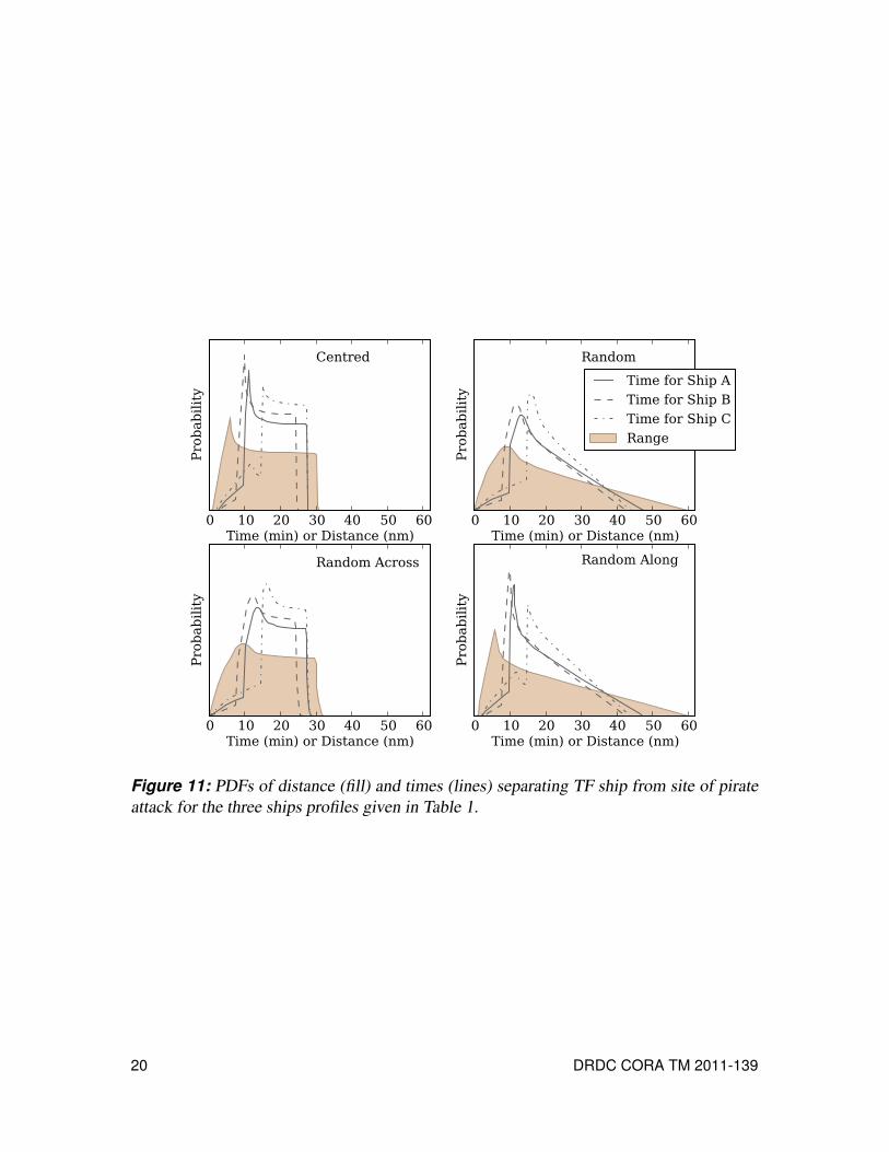
is considered (Figure 11), the PDFs become more complicated as the TF asset capabilities

come into effect. If the asset had a constant response time (e.g. constant ship transit speed

with no helicopter), then the mapping from distance to time simply causes the distance PDF

to be stretched by (1/vship). Because the launching of a helicopter increases the distance

covered in a given time by a considerable amount, there is a step-like increase in the PDF

when the helicopter is launched.

45. It is interesting to note that once the range is larger than the distance across the IRTC,

there is only a small discrepancy between the Centred and the Random Across patrol strate-

gies, and also only a small discrepancy between the Random and Random Along patrol

strategies. This result suggests that, so long as the shape of the PA is rectangular, with the

width across the region smaller than the length, the location of the TF ship across the PA

is not important in determining response times. This finding is an important factor when

applying the 1D model.


0 10 20 30 40 50 60Time (min) or Distance (nm)

Probability

Centred


Probability

Random

Time for Ship A

Time for Ship B

Time for Ship C

Range


Probability

Random Across


Probability

Random Along

Figure 11: PDFs of distance (fill) and times (lines) separating TF ship from site of pirate

attack for the three ships profiles given in Table 1.


3.2 Identifying the likelihood of a 30-minute responsetime

46. A key metric presently used to assess the effectiveness of patrols is the ability to

respond to an event within 30 minutes. (Note that while τ = 30 minutes is used here, for

operational purposes related to CP in the GOA, the value could be set to an arbitrary value

without altering the computational expense.) This section discusses how to answer the

question, “Given a ship with some capability that is covering a patrol box of length L, what

is the likelihood that an event will be intercepted within 30 minutes?”

47. To answer this question, the 2D models require integration of PDFs like those shown

in Figure 11 to identify what portion of a region can be covered within the time limit. By

comparison, the 1D model gives simple equations that can be solved quickly (see below),

making them useful for optimization problems.

48. Figure 12 shows the probability of Ship A intercepting an incident within 30 minutes

or less. Calculations based on the uncorrected 1D model are shown as dotted lines, and the

results scaled by the error overestimation factors are shown as dashed lines. The symbols

represent values calculated using the 2D models. The results for the same ship but with no

helicopter are shown in Figure 13.

49. Consistent with Figure 9, Figures 12 and 13 indicate that the over-estimation factor is

more important when short distances are being considered. In Figure 12, the error correc-

tion is larger for the RAC patrol than the RAL patrol. This result matches Figure 9, where

ships traveling across the IRTC will require greater correction than those that do not.

50. Benchmarking performed on the effort required to generate Figures 12 and 13 show

that the 1D model is well over four orders of magnitude faster than the 2D models. This

factor, combined with the goodness of fit between the 1D and 2D models permits us to

now move forward using the 1D model with greater confidence to consider more complex

location-allocation problems.

3.3 Coordinating Multiple TF Assets

3.3.1 Assigning Patrol Boxes to Optimize Response

51. In the above section, it is shown that the 1D model can provide the likelihood of a

TF ship responding to an incident in its PA within a given time limit provided that the

ship characteristics, the patrol box length, and the patrol strategy are known. From here it

becomes possible to optimize the response of multiple ships that must divide a given patrol

area such as the IRTC.


0 30 60 90 120 150 180Length of Patrol Box (nm)

0.0

0.2

0.4

0.6

0.8

1.0

ProbabilityofRespondingWithin

30Minutes

Random Along (2D)

Random Across (2D)

Centred (1D)

Random (1D)

Centred (1D), corrected for error

Random (1D), corrected for error

Figure 12: Model comparison of response capabilities for Ship A, given a 30-minute re-

sponse window.


0 30 60 90 120 150 180Length of Patrol Box (nm)

0.0

0.2

0.4

0.6

0.8

1.0


30Minutes

Random Along (2D)

Random Across (2D)

Centred (1D)

Random (1D)

Centred (1D), corrected for error

Random (1D), corrected for error

Figure 13: Model comparison of response capabilities for Ship A without a helicopter,

given a 30-minute response window.


Figure 14: Dynamic positioning of Ship A based on location of Ship B.

52. For demonstration purposes, consider two ships that collectively patrol a 150 nm-long

region of the IRTC with a length. A simplified allocation problem could be the following:

for Ships A and B listed in Table 1, if Ship A has a centred patrol strategy and Ship B has a

random patrol strategy, how will ship positioning affect probability of intercepting a pirate

attack?

53. Ship A can position itself using one of two possible approaches. In the first, it assumes

a static location, which is to say that if Ship B is assigned a PA with a length LB, Ship A

will position itself in the middle of a PA with length LA = L−LB. This approach is defined

as static positioning. In the second, Ship A considers the current position of Ship B and

positions itself in a manner that maximizes the overall response capabilities of both ships.

This approach is defined as dynamic positioning.

54. A definition sketch for the dynamic positioning scenario is provided in Figure 14. In

the figure, the distances ΔxA and ΔxB are defined so that both ships can reach their shared

patrol-box edge in the same amount of time 7. Mathematically, the position of Ship A is

found by solving

ΔxB +2ΔxA = L− xB (6)

where for Ships A and B, the Δx value is defined as

Δx =

⎧⎨⎩

vst t ≤ th

vsth + vh(t− th) t > th(7)

with vs, vh, and th defined based on the individual ships and t set to same value for both

ships. Noting that Equation (7) is really two equations (one for Ship A and one for Ship B),

Equations (6) and (7) provide a system of three equations to solve for the three unknowns

ΔxA, ΔxB, and t.

55. If it is assumed that Ship A will shadow the movements of Ship B in a dynamic fashion

so that the above equations remain satisfied, the average coverage capabilities can be found

by averaging the ship response capabilities over the possible values of xB (which range

from 0 to LB).

7. In cases where a there is uncertainty in the helicopter launch delay time, this shared edge would be

based on the average response capabilities.


0 20 40 60 80 100 120 140Patrol Box Length for Ship B

0.0

0.2

0.4

0.6

0.8

1.0

Probabilityofinterceptionwithin

timelimit

20 minutes - static

20 minutes - dynamic

30 minutes - static


40 minutes - static


Figure 15: Response capabilities for a two-ship problem.

56. The effect of static or dynamic positioning on overall response effectiveness is shown

in Figure 15 for response windows of 20, 30, and 40 minutes. For all patrol box sizes, the

response capabilities are improved when the PA for Ship A is varied dynamically based

on the location of Ship B (statistics are provided in Table 3). While dynamic positioning

does not alter the outcome if the assets are positioned in an optimal manner to begin with,

it mitigates the effects of poor positioning considerably. Hence, if this example is used

to consider the problem of managing patrol strategies near a ship that does not coordinate

with the major coalitions, this approach delivers a method to position coalition ships in a

manner that utilizes position of the uncoordinated ships in an optimal manner.

3.3.2 Considering Helicopter Readiness

57. Helicopters waiting to launch will remain at high alert states for short periods of time,

returning to lower readiness levels for most of the time. In this section, the effect of he-

licopter readiness on dynamic asset allocation is examined with the following model. A

three-ship problem was considered, under the following assumptions:


Table 3: Statistics for optimal patrol box sizes for Ships A and B covering a 150 nm section

of the IRTC.

20 min. Response 30 min. Response 40 min. Response

Static Dynamic Static Dynamic Static Dynamic

Ship A PA Length 40 nm Variable 70 nm Variable 95 nm Variable

Ship B PA Length 110 nm 90 nm 80 nm 55 nm 55 nm 60 nm

Max(P Intercept) 52% 53% 85% 87% 100% 100%

Min(P Intercept) 27% 40% 46% 62% 61% 74%

Mean(P Intercept) 45% 49% 68% 77% 84% 92%

a. The helicopters on these ships can have one of two readiness levels, high (H) and

low (L). At the high readiness level a helicopter can be launched within 5 minutes,

while at the lower readiness level it will take 15 minutes to launch.

b. A helicopter may remain at a heightened alert level for one shift, after which it must

be stood down to a lower level for at least two shifts. (The length of the shift does

not matter, so long as all shifts are of equal length.)

c. The length of PAs can be coordinated (i.e. the assets with helicopters at high-alert

cover a larger area) or uncoordinated (all assets cover an equal area).

d. The asset that can reach the location of the incident the fastest will respond.

e. The combined patrol area is set such that when two helicopters are at heightened

alert and one at the lower alert level, it is possible to coordinate PAs so that the entire

region can be covered in 30 minutes or less.

f. At any given time, the three ships can exhibit one of six possible readiness states that

can fit into one of four categories 8:

(a) All helicopters at high alert level (HHH)

(b) Two helicopters at high alert level

Low-alert helicopter on end of patrol box (HHL or LHH)

Low-alert helicopter in centre of patrol box (HLH)

(c) One helicopter at high alert level

High-alert helicopter on end of patrol box (HLL or LLH)

High-alert helicopter in centre of patrol box (LHL)

(d) All helicopters at low alert level (LLL)

58. Results for the various readiness levels are shown in Figure 16 and are grouped into

two sets. On the left, the six permutations of helicopter readiness are shown. On the

right, the average response for combinations of three successive “rotations” of readiness

are presented. For the permutations of possible readiness levels among the three assets, the

8. Note that HHL and LHH are the same for modeling purposes, as are LLH and HLL.


HHH

HHL

HLH

LLH

LHL

LLL

HHH,LLL,LLL

HHL,LLH,LLL

LHL,H

LH,LLL

HLL,LHL,LLH

Readiness Level (High/Low)

0.0

0.2

0.4

0.6

0.8

1.0


Tim

eLim

it

20 min Uncoordinated

20 min Coordinated

30 min Uncoordinated

30 min Coordinated

Figure 16: Effect of helicopter readiness on response capabilities.

configurations HHH, HHL and HLH all have the ability to cover 100% of the patrol area in

30 minutes or less if the assets coordinate their positioning. However, these combinations

are not sustainable, and lower readiness combinations would need to be included in any

cycle. For any set of cycles that maximizes the number of high-readiness rotations, 30-

minute coverage capabilities are in the range of 84% to 88%. For a shorter time limit of 20

minutes, the patrolled domain is too big relative to the response distances of the assets for

there to be benefit to asset coordination.

59. Based on these findings, it appears that it is likely that helicopter readiness levels

should be based on times and locations of elevated pirate activities and higher commercial

traffic density, rather than the readiness levels of nearby ships. To be certain, however,

this result would need to be sought using data that reflected the actual positioning and

capabilities of TF assets.


3.4 Altering Ship Position to Compensate for Wind60. Discussions with analysts from fellow TTCP nations indicated that some operators

have expressed concerns that asset allocation tools being prepared for these types of patrols

should be able to compensate for wind. While wind can affect asset positioning within its

PA, simple modeling efforts indicate that winds in the GOA should not greatly affect the

size of a patrol box that may be covered by a TF asset. This finding was identified by

calculating how wind affects the bearing a helicopter must follow to reach a target as well

as the resulting helicopter velocity over ground. Using a sine law condition, it can easily

be shown that the bearing of the helicopter needs to be adjusted by an amount

θh =−arcsin

(vwind

vhelosinθw

)(8)

where vwind is the wind speed and θw is the direction of the wind relative to the direction

to the target. For example, if the wind is blowing at 25 kts in a direction 20 degrees to

the right of the intended direction of travel, then a helicopter with a transit speed of 90 kts

would need to follow a bearing 5.5 degrees to the left of the intended direction of travel to

arrive at its desired destination. The effective speed of the helicopter is also changed to

vhelo = vhelo cosθh + vwind cosθw, (9)

which permits the travel time along the adjusted vector to be calculated as well.

61. Winds blowing at 30 to 40 kts are likely to be associated with a Sea State of 5. Such

conditions will include waves that are too energetic for pirates to engage in ship-boarding

activities. If winds are this strong counter-piracy patrols are probably not necessary. Thus,

to test whether winds can considerably alter coverage capabilities under relevant condi-

tions, examining winds at this strength are sufficient.

62. Two base cases of winds blowing along or across the IRTC are examined, noting that

any other direction can be considered a combination of these two. Figure 17 shows the

results for the four pairings of wind speed (30 kts or 40 kts) and direction (along or across

IRTC). In the figure, the black dot and black circle show ship location and the 30-minute

coverage limit for Ship A in the absence of wind. The red dot and dashed red circle show

adjusted ship position and resulting the patrol coverage capability under windy conditions,

where the ship position is shifted upwind by a distance

vwind(τ− th), (10)

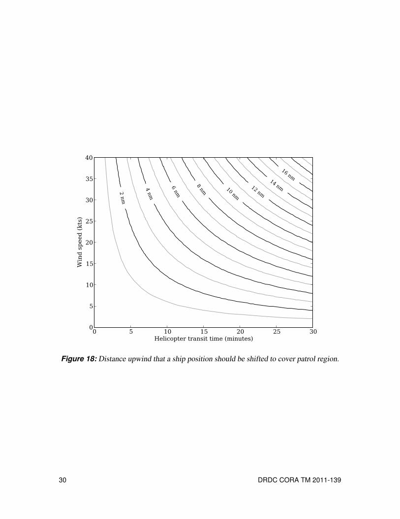
where τ − th is the transit time for the helicopter. The distance upwind that a ship should

be positioned is shown in Figure 18, which may be interpreted as follows. If a response

time of τ = 30 minutes is required and the helicopter launch delay is th = 10 minutes, then

τ − th = 20 minutes. Drawing a vertical line on the graph at this value shows how far

the ship position should be shifted as a function of wind speed. For example if the wind


Figure 17: Compensation of ship location to account for wind.

speed is vwind = 15 kts, then to cover the same region that it would cover under windless

conditions, the ship should reposition itself 5 nm upwind.

63. Based on these results, the effects of wind can be expected to alter the positioning of

a ship, but not necessarily its ability to effectively cover the region of interest.


0 5 10 15 20 25 30Helicopter transit time (minutes)

0

5

10

15

20

25

30

35

40

Windspeed(kts)

2nm

4nm

6nm

8nm 10

nm

12nm

14nm

16nm

Figure 18: Distance upwind that a ship position should be shifted to cover patrol region.


4 Findings, Recommendations and FutureWork

4.1 Findings64. The modeling effort undertaken in this work revealed several key findings for assets

patrolling long thin regions:

a. The 1D patrol coverage model can adequately identify the likelihood of a ship in-

tercepting a target based on the size of the patrol box and the patrol strategy but it

cannot give a probability distribution of response distances or response times. As

a result the choice of patrol coverage model will depend on the desired measure of

effectiveness.

b. In cases where 1D model is sufficient, it is the preferred option as it requires less

than 0.01% of the time to perform its calculations (a few seconds rather than several

minutes).

c. In responding to incidents that occur at random locations with their PA, assets centred

within their PA consistently outperform assets that travel randomly through them.

d. The position of an asset across a long and thin PA has little effect on response capa-

bilities compared to its position along its length.

e. A heterogeneous fleet (various assets with differing capabilities) will be more effec-

tive at covering a region if the length of PAs are customized to match the capabilities

of the individual assets.

f. In cases where all asset taskings are not or cannot be optimized to match capabilities,

dynamic positioning of the assets that can be tasked as needed can enhance response

effectiveness considerably.

g. A fleet that places ship helicopters on heightened alert in a coordinated fashion mayonly mildly outperform a fleet that lets individual ships control their helicopter readi-

ness levels, depending on the size of the patrol region.

h. While wind affects helicopter transit speeds over ground, a ship can position itself

within its PA to accommodate the effect.

4.2 Recommendations65. The modeling presented here lays forth several recommendations for allocating assets

to patrol a long and thin region such as the IRTC in the GOA. These include:

a. PAs should be defined in a manner that considers the response capabilities of the

individual assets. For example, a ship with a fast helicopter will be able to cover a


larger area than a ship with a slower helicopter or no helicopter at all, and the size of

PAs should be assigned accordingly based on the range an asset can cover in a given

amount of time (see Equation (4)).

b. Assets should remain as close to the centre of their PA as possible to maximize re-

sponse effectiveness. This strategy will minimize the number of assets required to

patrol the entire corridor. If ship movement is desired to develop situational aware-

ness, dynamic PAs should be used to keep assets centred in their PA. In addition,

assets should patrol the regions in a coordinated fashion, keeping the along-channel

distance between ships relatively constant.

c. In cases where the operations of one asset do not permit it to remain at the centre of

its PA, adjacent assets should alter their position and PA in a dynamic fashion based

on the real-time position of the other asset. This dynamic approach to positioning

will improve patrol coverage effectiveness.

d. Following the findings in Section 3.3.2, the possibility that ships should place he-

licopters at heightened alert based on the locally-perceived risk of pirate activity

(rather than in a coordinated effort that maintains an steady average readiness for the

entire fleet) should be examined using a realistic example.

e. In windy conditions, ships should reposition themselves upwind by a distance that

is based on helicopter speed, wind speed, time delay for helicopter launch, and de-

sired response-time window. The desired distance can be extracted from Figure 18,

following the example provided at the end of Section 3.4.

4.3 Future Work: Proposed Allocation Model66. At present, executing these recommendations is a challenge as there is no readily

available tool for analysts and operators who are setting the patrol schedules. Hence, the

next step is to synthesize the findings presented in this report to produce an operationally

useful asset position and allocation model. The model should include the ability to consider

multiple ships with individual capabilities. Two modes of utilization would be beneficial.

The first would be a planning mode that used anticipated asset availability to suggest where

along the IRTC the assets should be positioned. The second would be a more responsive

mode that suggested “fine-tuning” of asset positions as perceived risks and asset availability

evolved.

67. The logical structure of such a model could be as follows. Consider a set of I ships

assigned to patrol a section of a corridor of length L. Each ship will have the properties

ship speed (vship)i, helicopter speed (vhelo)i, and an expected helicopter launch delay (th)i.

Combined, these features will provide a representative response curve ρi(r) that describeshow long it takes for a vessel with its helicopter to reach an incident some distance r away.

This response curve can be calculated with the 1D model.


68. Further, these ships can be subdivided into two categories: ships are under direct

coalition command (group M), and ships in the region that are performing counter-piracy

duties outside of coalition control (group N). If ship i is within group M, then Mi = 1 and

Ni = 0, otherwise Mi = 0 and Ni = 1. Since these groups are exclusive of each other, it is

necessary that Mi +Ni = 1 and

∑i∈I

Mi +Ni = I. (11)

69. Each ship may be assigned to a location xi, where 0 ≤ xi ≤ L. For ships in group N,

this position is known, e.g. through observation, but cannot be changed since the ship is

outside coalition command. For ships in group M, the values of xi are found in a manner

that minimizes

F =∫ L

0Rρmindx (12)

where R = R(x, t) is the risk function that defines the likelihood of an attack occurring

at a particular location 9, and ρmin = ρmin(x) is the shortest response time for any of the Iassets to reach the location x, i.e.

ρmin(x) =min(ρi(x)). (13)

Note that the dependency of R on time implies that the value of F and therefore the optimal

position of ships is likely to vary in time.

70. For scenarios where the ships are positioned and must adjust after one gets tasked

or becomes otherwise occupied, readjustment of the positions would be performed in a

manner that minimized repositioning the ships. For example, if the ship order is A, B, C,

D, E and Ship D must remove itself from general patrol, the dynamic allocation model

would give the best coverage for the remaining ships, ensuring that the order remains as A,

B, C, E. If at some later time, Ship D were to become available once again but its location

was between Ships B and C, then the dynamic allocation model would find the optimal

positioning that kept the ship ordering as A, B, D, C, E.

71. It would also be beneficial to couple the proposed model with a reconnaissance tool

that considered how changing ship patrols affected the quality of the regional maritime

picture and whether making such changes would alter the requirements for other assets

such as maritime patrol aircraft.

9. For the counter-piracy problem, the risk index value is likely to be determined based on the locations

of recent incidents pirate activity, locations of suspected pirates, density of merchant ships that are at risk

of high-jacking, and meteorological/oceanographic considerations such as wind and waves. This term is

beyond the scope of the proposed modeling effort but could be based on ongoing and future analyses of

coalition allies and TTCP partners.


References

[1] Mirshak, Ramzi (2009), The Gulf of Aden Anti-Piracy Planning Tool (GAPP), v 1,

(DRDC CORA LR-2009-055) Defence R& D Canada – CORA. UNCLASSIFIED.

[2] Mirshak, Ramzi (2010), The Gulf of Aden Anti-Piracy Planning Tool (GAPP), v 3.1,

(DRDC CORA LR-2010-155) Defence R& D Canada – CORA. UNCLASSIFIED.

[3] Black, Robert (2009), Information Needs and Awareness: Predictive & Reactive

Timeliness. Brief presented to Working Group 5 of the MORS Special Meeting on

Maritime Domain Awareness and Counter-Piracy.

[4] Kraska, James and Wilson, Brian (2009), Combating the Pirates of the Gulf of Aden:

Collaboration, Not Kinetics, Ocean and Coastal Management,p. doi:10.1016/j.ocecoaman.2009.07.002.

[5] Ploch, Lauren, Blanchard, Christopher M., O’Rourke, Ronald, Mason, R. Chuck,

and King, Rawle O. (2009), Piracy off the Horn of Africa. Congressional Research

Service Report for Congress.

[6] Nicoll, Alexander and Johnstone, Sara (2009), Combating Piracy off Somalia: Swift

naval response is only part of the solution, IISS Strategic Comments, 15(1).

[7] Unprecedented Increase in Somali pirate activity (online), www.icc-css.org/index.php?option=com_content&view=article&id=376:uprecedented-increase-in-somali-pirate-activity&catid=60Lnews&Itemid=51 (Access Date: 3 June 2010).

[8] Best Management Practices to Deter Piracy in the Gulf of Aden and off the Coast of

Somalia (online), www.marisec.org/piracy-gulf-of-aden-indian=ocean-industry-best-management-practice (Access Date: 3 June

2010).

[9] Kraska, James (2009), Coalition Strategy and the Pirates of the Gulf of Aden and the

Red Sea, Comparative Strategy, 28, 197–216.

[10] Marsaglia, George, Narasimhan, B., and Zaman, Arif (1990), The distance between

random points in rectangles, Commun. Statist.-Theory Meth., 19(11), 4199–4212.

[11] Freund, John E. (1971), Mathematical Statistics, Second ed, Prentice-Hall.

[12] Abramovitz and Stegun (1964), Handbook of Mathematical Functions, McGraw

Hill.


Annex A: Response-Time Uncertainties

A1. The models presented in Section 2 determine the probability distributions of response

distance, then convert the results to response times based asset transit speed, which de-

pends on the delay in helicopter launch th. This annex discusses how uncertainties in the

helicopter launch delay can be incorporated to improve estimates of response delays.

A.1 Time Required to Cover a Known DistanceA2. Uncertainty in launch delay affects asset transit speed v. If the helicopter will launch

after some known time th, the function for v will have a step function where

v(r) =

⎧⎨⎩

vship r ≤ vshipth

vhelo r > vshipth(A.1)

Also, the time necessary for an asset to reach a range r is

τr =

⎧⎪⎪⎪⎨⎪⎪⎪⎩

rvship

th ≥ rvship

rvhelo

+ th

(1− vship

vhelo

)th <

rvship

(A.2)

A3. However, if the launch delay is not constant but instead fits a probability density

function th ∼ Ph(t), then the mean transit speed as a function of distance will follow the

more generalized form 10,

v(r) = vhelo

∫ r

0Ph

(r′

vship

)dr′+ vship

∫ ∞

rPh

(r′

vship

)dr′. (A.3)

and the mean time required to reach a target a distance r away is

τr =∫ r

0

drv. (A.4)

Note that this is the mean response time: it does not give information about the distribution

of response times. By inserting Ph(t) into (A.2) and observing that to reach a target a

distance r away in a time τ requires the launch delay to be

t∗h =vheloτ− r

vhelo− vship, (A.5)

10. Note that for normal distributions (like those used in GAPP), the integrals in this equation will have an-

alytical solutions that make use of the error function and complementary error function (see, e.g., Abramowitz

and Stegun [12] for more information on these functions).


the distribution of response times at a distance r away is found to fit

τr ∼ P∗h (t∗h) (A.6)

where

P∗h (t∗h) =

⎧⎪⎪⎪⎪⎪⎪⎪⎪⎪⎨⎪⎪⎪⎪⎪⎪⎪⎪⎪⎩

0 t∗h >r

vship

∫ ∞

r/vship

Ph dt t∗h =r

vship

Ph(t∗h) t∗h <r

vship

(A.7)

A4. Generic values of average transect speed and response time PDFs are shown in Fig-

ure A.1. The figure assumes helicopter launch delays fit a normal distribution and compares

results from the theoretical curves defined above with results from a GAPP-style algorithm,

showing good agreement. The top panel, which shows transit speed, follows the shape of

a scaled error function, as is expected for a normal distribution. The bottom panel shows

response-time curves for different four distances and is useful for understanding (A.7). In

the first two response time panels, the ship commonly arrives on scene before the helicopter

has had time to launch. For cases where the helicopter launches before arrival on scene, the

response-time curve fits part of a bell-curve. However, any times where the launch would

have been after the ship already arrives on scene get binned together, resulting in a spike

of probability at a time that matches when the ship arrives on scene. In the last two panels,

the helicopter always launches before the ship arrives on scene, so the response time fits a

distribution like that of the helicopter launch delay.

A5. Examples of v(r) for these two cases are shown in Figure A.2. The figure shows cases

for the three ships listed in Table 1, with and without an uncertainty in launch time. For

the solid line, there is no variability in the launch time, while for the dashed line the launch

time is extracted from a normal distribution with a standard deviation of σth = 3 minutes.

A.2 Distance Covered in a Known TimeA6. The range covered in a time τ is

rτ =

⎧⎨⎩

vshipτ τ ≤ th

vheloτ− (vhelo− vship

)th τ > th

(A.8)


vs(t

h−σ

t) v

sth

vs(t

h+σ

t)

Range Travelled

0

vs

vh

AverageTransitSpeed

Monte Carlo (4000 Iterations)

Theory

th

2th

Time

Probability

r=vs(t

h−2σ)

th

2th

Time

r=vs(t

h−σ)

th

2th

Time

r=vsth

th

2th

Time

r=vs(t

h+σ)

Figure A.1: Average transit speed for a helicopter with normally distributed launch delay

(top panel), and representative response times (bottom panels).


0 2 4 6 8 10 12 1420

40

60

80

100Ship A

thknown exactly

thwith σ

th=3 min.

0 2 4 6 8 10 12 1420

40

60

80

100

Assettransitspeed(kts)

Ship B

0 2 4 6 8 10 12 14Range (nm)

20

40

60

80

100Ship C

Figure A.2: Velocity profiles for 2D model using exact and probabilistic treatments to

helicopter launch time.


Thus, when the launch delay follows th ∼ Ph(t), the range covered follows

rτ ∼ Pτ(r) =

⎧⎪⎪⎪⎪⎪⎪⎪⎪⎪⎨⎪⎪⎪⎪⎪⎪⎪⎪⎪⎩

0 τ >r

vship

∫ ∞

rvship

Phdt τ = rvship

Ph (t∗h) τ <r

vship

(A.9)

A.3 Covering a Known Distance in a Known TimeA7. The likelihood that an asset can reach a range r within a time τ is

P(r,τ) =

⎧⎪⎪⎪⎪⎪⎪⎨⎪⎪⎪⎪⎪⎪⎩

1 r ≤ vshipτ

∫ t∗h

0Ph(t) dt vshipτ < r ≤ vheloτ

0 r > vheloτ

(A.10)

Figure A.3 shows results when τ = 30 minutes for the three ships in Table 1.

A.4 Application to 2D modelsA8. In the absence of any uncertainty in the helicopter launch delay, conversion of the

probability density function f (r) to response time g(t) is calculated as [11]

g(t) = f (r)∣∣∣∣drdt

∣∣∣∣= v f (r) (A.11)

where v = v(r) is the asset speed at range r. When the launch delay th is known exactly,

v is known exactly at all times/distances, which makes (A.11) easy to solve. However,

incorporation of variability in helicopter launch time will affect the PDF and the probability

function becomes

g(τ) =∫ ∞

0f (r)P∗h (t

∗h)dr. (A.12)

A9. An example of this transformation is shown in Figure A.4. The figure applies the

helicopter launch profile of Ship A (with a standard deviation of σ = 3 minutes) to the

distance PDF of the Random patrol strategy shown in Figure 10. In Figure A.4, the bottom

panel reproduces the distance PDF shown in Figure 10. The centre panel shows a contour


0 10 20 30 40 50

0.0

0.2

0.4

0.6

0.8

1.0Ship A

thknown exactly

thwith σ

th=3 min.

0 10 20 30 40 50

0.0

0.2

0.4

0.6

0.8

1.0

Probabilitythatassetcanreachrange

Ship B

0 10 20 30 40 50Range (nm)

0.0

0.2

0.4

0.6

0.8

1.0Ship C

Figure A.3: 30-minute range of various assets.


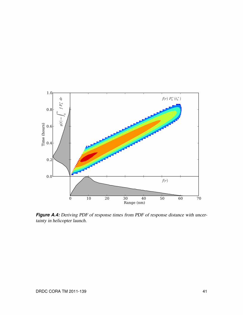
0 10 20 30 40 50 60 70Range (nm)

f(r)

f(r) P ∗

h (t ∗h )

0.0

0.2

0.4

0.6

0.8

1.0

Tim

e(hours)

g(t)=

∫ ∞ 0

fP∗ hdr

Figure A.4: Deriving PDF of response times from PDF of response distance with uncer-

tainty in helicopter launch.


plot f (r)P∗h on a log scale (with values less than 1 in a million being masked). The left

panel shows the result of (A.12), i.e. integrating the contour plot along lines of constant t.

A.5 Application to 1D ModelA10. When the exact launch time is not known, the probability of reaching a target in a

domain of length L in a time τ can be described by

Pc(L,τ) =∫ L/2

0

2rL

P(r,τ)dr+∫ ∞

L/2P(r,τ)dr (A.13)

for the Centred-1D approach and

PR(L,τ) =∫ L/2

0

2rL

(L− r

2

)P(r,τ)dr+

∫ L

L/2

rL

(2− r

L

)P(r,τ)dr+

∫ ∞

LP(r,τ)dr (A.14)

for the Random-1D approach, where P(r,τ) is defined in (A.10).

A.6 Other Time DelaysA11. Although not discussed in the demonstrations used here, other delays may also be

incorporated in identifying the total response time. For example, GAPP also permits one

to consider the time required for commercial vessels to broadcast that they are under attack

(which we will assume has the PDF R(t)) as well as the time required a ship to begin

its response from when it learns of the attack (which we will assume has the PDF S(t)).Incorporating these effects gives a total response time PDF

g(t) = g(t)∗R(t)∗S(t) (A.15)

where ∗ is the convolution operator.


Annex B: Radial Propagation Algorithm

B1. This annex describes the radial propagation algorithm that provides an alternative to

the Marsaglia et al. [10] approach. The premise is that the proportion of a rectangular PA

of area A that is some range r from an asset is

f (r) =Δθ r δ r

A(B.1)

where Δθ is the arc of a circle of radius r that passes through the patrol region (Figure 4)

and δ r is an infinitesimally small width.

B2. In presenting the approach, it is assumed that the asset is positioned at one edge of

the patrol area and is either outside the patrol area or bordering it. To consider cases where

the asset is somewhere along the length of the patrol area, or inside it, it is necessary to

break the problem into components. The left panel of Figure B.1 shows a situation where

the asset is within the PA, making it necessary to divide the PA into four sections with the

asset at a point where the four sections meet.

B.1 Calculation of PDFB3. The PDF itself is calculated as f = f (r,h1,h2, �) where h1 and h2 are the lower and

upper bounds of the region and � is the length (see the right panel of Figure B.1 for a

definition sketch). The region of interest can have one of two possible configurations. In

the first (Case 1), the rectangle is long and thin, such that h22 ≤ �2+h2

1. In the second (Case

2), the rectangle is short and wide, such that h22 > �2+h2

1.

B4. For Case 1, the PDF is described by inserting the following definition of Δθ into

(B.1):

Δθ(h1,h2,r, �) =

⎧⎪⎪⎪⎪⎪⎪⎪⎪⎪⎪⎪⎪⎪⎪⎪⎪⎪⎪⎪⎨⎪⎪⎪⎪⎪⎪⎪⎪⎪⎪⎪⎪⎪⎪⎪⎪⎪⎪⎪⎩

0 r < h1

π2− arcsin

(h1

r

)h1 ≤ r < h2

arcsin

(h2

r

)− arcsin

(h1

r

)h2 ≤ r <

√�2+h2

1

arcsin

(h2

r

)− arccos

(�

r

) √�2+h2

1 ≤ r ≤√

�2+h22

0 r >√�2+h2

2

(B.2)


Along Corridor

AcrossCorridor

Along Corridor

AcrossCorridor

�

h1

h2

Figure B.1: (Left) Division of Patrol Area based on asset position. (Right) Dimensions

used in calculations.

For Case 2, the definition of Δθ is

Δθ(h1,h2,r, �) =

⎧⎪⎪⎪⎪⎪⎪⎪⎪⎪⎪⎪⎪⎪⎪⎪⎪⎪⎪⎪⎨⎪⎪⎪⎪⎪⎪⎪⎪⎪⎪⎪⎪⎪⎪⎪⎪⎪⎪⎪⎩

0 r < h1

π2− arcsin

(h1

r

)h1 ≤ r <

√�2+h2

1

π2− arccos

(�

r

) √�2+h2

1 ≤ r < h2

arcsin

(h2

r

)− arccos

(�

r

)h2 ≤ r ≤

√�2+h2

2

0 r >√

�2+h22

(B.3)

B.2 Application to Patrol StrategiesB5. The symmetry embedded in the patrol strategies and IRTC layout are used to reduce

number of calculations required to identify f . For example, for the centred patrol strategy

the region is bisected along the minor axis of the rectangle, so it is only necessary to

calculate the distribution for one half of the region. Similarly, the symmetry of the IRTC

requires that only one of the two lanes requires consideration. The results calculated with

this approach are identical to those calculated by the Marsaglia et al. approach in Figure

10.


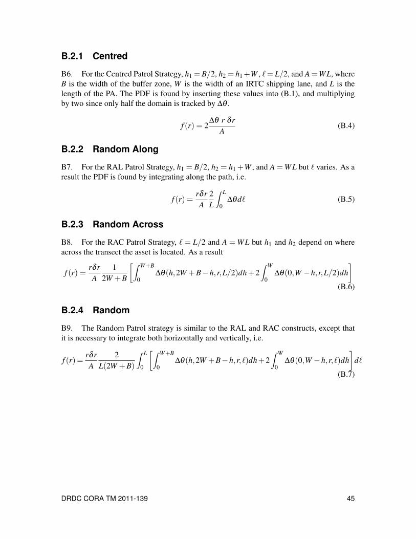
B.2.1 Centred

B6. For the Centred Patrol Strategy, h1 = B/2, h2 = h1+W , �= L/2, and A=WL, where

B is the width of the buffer zone, W is the width of an IRTC shipping lane, and L is the

length of the PA. The PDF is found by inserting these values into (B.1), and multiplying

by two since only half the domain is tracked by Δθ .

f (r) = 2Δθ r δ r

A(B.4)

B.2.2 Random Along

B7. For the RAL Patrol Strategy, h1 = B/2, h2 = h1+W , and A =WL but � varies. As a

result the PDF is found by integrating along the path, i.e.

f (r) =rδ rA

2

L

∫ L

0Δθd� (B.5)

B.2.3 Random Across

B8. For the RAC Patrol Strategy, � = L/2 and A = WL but h1 and h2 depend on where

across the transect the asset is located. As a result

f (r) =rδ rA

1

2W +B

[∫ W+B

0Δθ(h,2W +B−h,r,L/2)dh+2

∫ W

0Δθ(0,W −h,r,L/2)dh

]

(B.6)

B.2.4 Random

B9. The Random Patrol strategy is similar to the RAL and RAC constructs, except that

it is necessary to integrate both horizontally and vertically, i.e.

f (r)=rδ rA

2

L(2W +B)

∫ L

0

[∫ W+B

0Δθ(h,2W +B−h,r, �)dh+2

∫ W

0Δθ(0,W −h,r, �)dh

]d�

(B.7)


Annex C: Theory of Marsaglia et al. (1990)

C1. This annex provides an overview of the theoretical results presented by Marsaglia

et al. [10] that are used to develop the 2D response model. Their work considers the

probability distribution of the square of the distance between two points in two random

rectangles of arbitrary size.

C2. The two rectangles (Rectangle A and Rectangle B) are described by their lengths

in the x and y directions, i.e. ax and ay for Rectangle A and bx and by for Rectangle B.

Note that in their analysis the sides of the rectangles are parallel to the x and y axes. The

spatial relationship between the two rectangles is identified by c= (cx,cy) that defines thetranslation vector required to get from the top-right corner of Rectangle A to the bottom-

left corner of Rectangle B (Figure C.1). Note that in the figure, both cx and cy are positive,

however they can be negative. By contrast, ax, ay, bx, and by are always positive. For

example, if one wished to identify the two random points in a square with sides of length �with this model, then ax = ay = bx = by = � and cx = cy =−�.C3. If the squared distance between two random points in the two rectangles is expressed

as r2, and the density of the square of the distances is f (r2), then

f (r2)=1

4axbxayby∑

i, j,k,l,m,n∈{0,1}

∫ r2

0(−1)i+ j+k+l

[(−1)m− q√

r2− x

]+

[(−1)n− s√

x

]+

dx

(C.1)

where q = cx + iax + jbx and s = cy + kay + lby, and the “plus” subscript indicates a spline

notation, i.e. Q+ =max(0,Q).

C4. Solving (C.1) requires the solution to four possible integrals:

I1 :

∫ r2

0

(1− q√

r2− x

)+

(1− s√

x

)+

dx = F (r2−q2+,s

2+,r

2,q,s)

I2 :

∫ r2

0

(1− q√

r2− x

)+

(−1− s√

x

)+

dx =−F (0,min((r2−q2+)+,s

2),r2,q,−s)

I3 :

∫ r2

0

(−1− q√

r2− x

)+

(1− s√

x

)+

dx =−F (0,min((r2− s2+)+,q2),r2,−q,s)

I4 :

∫ r2

0

(−1− q√

r2− x

)+

(−1− s√

x

)+

dx = F (min(r2,s2),(r2−q2)+,r2,−q,−s)

(C.2)


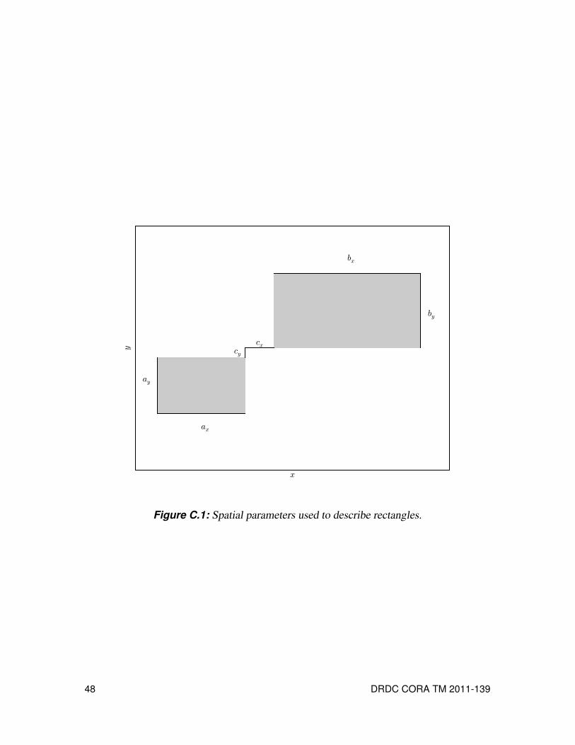
x

y

ax

ay

bx

by

cxcy

Figure C.1: Spatial parameters used to describe rectangles.


where

F (x1,x2,x3,x4,x5) =

⎧⎨⎩

0 x1 ≥ x2

G(x2,x3,x4,x5)−G(x1,x3,x4,x5) otherwise

(C.3)

and

G(y1,y2,y3,y4) = y1+2y3√

y2− y1−2y4√

y1+ y3y4 arcsin(2y1y2−1

). (C.4)

C5. It is noteworthy that both (C.2) and (C.4) have errors as presented in Marsaglia et al.

They also provide FORTRAN code that has a few small errors. In preparing the equations

given here, the Marsaglia model was tested heavily against the Monte Carlo and Ripple

Propagation approaches to ensure correctness. If one is to turn to the original paper, take

care when cross-referencing their equations with their code and with the equations provided

here.


Annex D: Error Calculations for 1D model

D1. The 1D model presented in this document estimates the part of the channel that a TF

asset can reach within a certain amount of time by identifying the range that the asset can

reach in that time, and then assuming that the total area is equal to the width of the channel

times the range. This approach ignores the circular nature of the range, a problem that is

illustrated in Figure 8.

D2. In Figure 8, the top panel shows a ship that is located just below a part of the channel

it is patrolling. The part of the channel assumed to be within its reach is traced out by a

rectangle (dotted line) that is a 2r long. Clearly from the figure, the model is overestimating

the response capabilities since there are parts of the rectangle that are outside the range that

can be reached by the asset. This section presents the theoretical analysis that allows the

degree of overestimation, shown in Figure 9, to be quantified.

D3. The results rely heavily on the calculation of the area of half circles (representing

half the ship range) cut by a horizontal line (representing the edge of a lane in corridor).

The two areas are shown as a function of the range r and the height of the line h in Figure

D.1 and defined as Ao and Ai.

D.1 Stationary Mode: Asset Remains CentredBetween Shipping Lanes

D4. For cases where the strategy is for the patrol to remain between the shipping lanes

(Stationary error correction), the area of a particular shipping lane that is within a range rdepends on the size of the circle (Figure D.2). The figure shows an asset (red dot) and two

IRTC lanes. Three circular regions are also depicted. In Region A, r < B/2. In Region B,

B/2 < r < W +B/2. In Region C, r > W +B/2. Thus, the actual area covered when the

ship remains between the two shipping lanes is

A =

⎧⎪⎪⎪⎪⎪⎪⎪⎪⎪⎨⎪⎪⎪⎪⎪⎪⎪⎪⎪⎩

0 r <B2

Ao

(r,

B2

)B2≤ r <W +

B2

Ai

(r,W +

B2

)−Ai

(r,

B2

)r ≥W +

B2

, (D.1)

and the correction factor for the actual area covered is

C =2rW

A. (D.2)


h

r

Ao =(πr2 )/2−Ai

Ai =θr2 +h√r2 −h2 , where θ=arcsin(h/r)

Figure D.1: Area calculations used to determine overestimation correction for 1D model.


Figure D.2: Calculating error correction when ship travels remains centred in corridor.

Note that, due to the symmetry of the problem, only one lane needs to be considered to

calculate the correction factor.

D.2 Across Mode: Asset Travels Across ShippingLanes

D5. When the patrol travels across the shipping lanes (Across error correction), the area

correction factor becomes more complex. It does remain symmetric, which simplifies cal-

culations since only one shipping lane needs to be considered. The geometrical construct of

the problem is shown in Figure D.3. Rather than having two areas as in the above problem,

there are now two integrals that need to be considered:

Ii(r,h1,h2) =∫ h2

h1

Ai(r,h)dh =

{r2[

harcsin(

hr

)+√

r2−h2

]− (r2−h2)1.5

3

}h2

h1

(D.3)


and

Io(r,h1,h2) =∫ h2

h1

Ao(r,h)dh =π2

r2 (h2−h1)− Ii(r,h1,h2). (D.4)

Tracing the path of the ship across the region shows that when the ship is traveling across

the corridor, the average area becomes A = A∗/(2WB), where

A∗ =

⎧⎪⎪⎪⎪⎪⎪⎪⎪⎨⎪⎪⎪⎪⎪⎪⎪⎪⎩

2Ii(r,0,r)+ Io(r,0,r)+πr2(W − r) r ≤W

2Ii(r,0,r)+ Ii(r,W,r)− Ii(r,0,r−W )+ Io(r,r−W,r) W < r ≤ L−W

2Ii(r,0,W )+ Ii(r,W,r)−2Ii(r,0,r−W )+2Io(r,r−W,L−W ) L−W < r ≤ L

2Ii(r,0,W )+ Ii(r,W,L)− Ii(r,0,L−W ) r > L(D.5)

so the correction term is once again

C =2rW

A. (D.6)

D.3 Range CoverageD6. As previously discussed, the 1D model treats the area covered as a rectangular region

with a width equal to the width of the corridor and a length equal to twice the range (as-

suming the ship is in the middle). This assumption neglects the radial spreading that takes

place. As a result, while this model is useful for identifying the likelihood of intercepting

an incident in a patrol region in a given amount of time, it does not produce reliable PDFs.

If PDFs are desired, a 2D model is preferable.


Figure D.3: Calculating error correction when ship travels across corridor.


List of Abbreviations UsedTerm Description

1D One Dimensional

2D Two Dimensional

AG Action Group

CMF Combined Maritime Force

CP Counter-Piracy

CTF Combined Task Force

EU NAVFOR European Union Naval Force, Somalia

GAPP Gulf of Aden Anti-Piracy Planning Tool

GOA Gulf of Aden

H High-readiness state

IMB International Maritime Bureau

IRTC International Recommended Transit Corridor

kts knots (nautical miles per hour)

L Low-readiness state

MAR Maritime Systems Group

min minutes

NATO North Atlantic Treaty Organization

nm nautical mile

PA Patrol Area

PDF Probability Density Function

RAC Random Across Patrol Strategy

RAL Random Along Patrol Strategy

TF Task Force

TTCP The Technical Cooperation Program


List of Mathematical Symbols UsedSymbol Description

ax Width of rectangle a in x-directionay Width of rectangle a in y-directionA Area

A∗ Average area

Ai Inner area of semi-circle cut by chord

Ao Outer area of semi-circle cut by chord

bx width of rectangle b in x-directionby Width of rectangle b in y-directionB Width of IRTC buffer zone

cx x-translation from upper-right corner of rectangle a to lower-left corner

of rectangle bcy x-translation from upper-right corner of rectangle a to lower-left corner

of rectangle bC Correction factor for 1D patrol models

f Probability density function

F Distribution function in Marsaglia et al. derivation

F Response function

g Probability density function

g Convolved probability density function

G Spline function in Marsaglia et al. derivation

h Shortest distance from circle-centre to chord crossing circle

i, j,k, l,m,n counters

I Number of ships considered in proposed asset allocation model

Ii Integral of AiIo Integral of Ao� Partial length of a patrol area

L Length of patrol area

M Set of ships under control of command

N Set of ships not under control of command

P(r,τ) Probability that an asset will be able to reach a range r in a time τPC(r,τ) Probability of responding to an incident a distance r away in a time τ

using a centred patrol strategy

Ph Probability that a helicopter will have launched by time t.P∗h Probability distribution for τrPR(r,τ) Probability of responding to an incident a distance r away in a time τ

using a random patrol strategy

q Distance variable in Marsaglia et al. derivation

[CONTINUED ON FOLLOWING PAGE...]


[... CONTINUED FROM PREVIOUS PAGE]

Symbol Description

r Distance or range covered by an asset

rτ Range covered by an asset in a time τR Distribution of time delay for a commercial vessel to announce attack

R risk function

s Distance variable in Marsaglia et al. derivation

S Distribution of time delay for an asset to begin response

t Time

th Time delay for helicopter launch

t∗h Time delay required for an asset to exactly cover a range r in a time τ(th)i Time delay for helicopter launch for asset i in proposed allocation model

v Transit speed

v Average transit speed

vhelo Helicopter transit speed

vhelo Helicopter transit speed corrected for wind

vship Ship transit speed

vwind Wind speed

W Width of IRTC shipping lane

xi Position of ship i in proposed asset allocation model

xB Fixed distance to edge of patrol area for ship B

x1,x2,x3,x4,x5 Dummy variables in Marsaglia et al. derivation

y1,y2,y3,y4 Dummy variables in Marsaglia et al. derivation

z Distance variable in Marsaglia et al. derivation

δ r Infinitesimal change in rΔxA, ΔxB Range from asset A or B to edge of patrol area shared by assets A and B

Δθ Arc

ρi response-time for asset iρmin minimum response-time

σth standard deviation of helicopter launch delay thθ angle

θH Change in helicopter azimuth

θw Wind direction relative to desired direction of travel

τ Response time

τr Time required to cover a range rτr Mean time required to cover a range r


DOCUMENT CONTROL DATA(Security classification of title, body of abstract and indexing annotation must be entered when document is classified)

1. ORIGINATOR (The name and address of the organization preparing thedocument. Organizations for whom the document was prepared, e.g. Centresponsoring a contractor’s report, or tasking agency, are entered in section 8.)

Defence R&D Canada – CORADept. of National Defence, MGen G.R. Pearkes Bldg.,101 Colonel By Drive, Ottawa, Ontario, Canada K1A0K2

2. SECURITY CLASSIFICATION (Overallsecurity classification of the documentincluding special warning terms if applicable.)

UNCLASSIFIED

3. TITLE (The complete document title as indicated on the title page. Its classification should be indicated by the appropriateabbreviation (S, C or U) in parentheses after the title.)

Ship Response Capability Models for Counter-Piracy Patrols in the Gulf of Aden

4. AUTHORS (Last name, followed by initials – ranks, titles, etc. not to be used.)

Mirshak, R.

5. DATE OF PUBLICATION (Month and year of publication ofdocument.)

September 2011

6a. NO. OF PAGES (Totalcontaining information.Include Annexes,Appendices, etc.)

76

6b. NO. OF REFS (Totalcited in document.)

12

7. DESCRIPTIVE NOTES (The category of the document, e.g. technical report, technical note or memorandum. If appropriate, enterthe type of report, e.g. interim, progress, summary, annual or final. Give the inclusive dates when a specific reporting period iscovered.)

Technical Memorandum

8. SPONSORING ACTIVITY (The name of the department project office or laboratory sponsoring the research and development –include address.)

Defence R&D Canada – CORADept. of National Defence, MGen G.R. Pearkes Bldg., 101 Colonel By Drive, Ottawa, Ontario,Canada K1A 0K2

9a. PROJECT NO. (The applicable research and developmentproject number under which the document was written.Please specify whether project or grant.)

PG11ia

9b. GRANT OR CONTRACT NO. (If appropriate, the applicablenumber under which the document was written.)

10a. ORIGINATOR’S DOCUMENT NUMBER (The officialdocument number by which the document is identified by theoriginating activity. This number must be unique to thisdocument.)

DRDC CORA TM 2011-139

10b. OTHER DOCUMENT NO(s). (Any other numbers which maybe assigned this document either by the originator or by thesponsor.)

11. DOCUMENT AVAILABILITY (Any limitations on further dissemination of the document, other than those imposed by securityclassification.)( X ) Unlimited distribution( ) Defence departments and defence contractors; further distribution only as approved( ) Defence departments and Canadian defence contractors; further distribution only as approved( ) Government departments and agencies; further distribution only as approved( ) Defence departments; further distribution only as approved( ) Other (please specify):

12. DOCUMENT ANNOUNCEMENT (Any limitation to the bibliographic announcement of this document. This will normally correspondto the Document Availability (11). However, where further distribution (beyond the audience specified in (11)) is possible, a widerannouncement audience may be selected.)

Unlimited

13. ABSTRACT (A brief and factual summary of the document. It may also appear elsewhere in the body of the document itself. It is highlydesirable that the abstract of classified documents be unclassified. Each paragraph of the abstract shall begin with an indication of thesecurity classification of the information in the paragraph (unless the document itself is unclassified) represented as (S), (C), (R), or (U).It is not necessary to include here abstracts in both official languages unless the text is bilingual.)

This work examines the capability-models of ships performing counter-piracy patrols in the Inter-national Recommended Transit Corridor, located in Gulf of Aden (GOA). Specifically, it considerspossible approaches to predict the response time of assets patrolling long and thin regions andto facilitate coordination between multiple assets.

For situations where the pirate attacks occur randomly, the across-channel location of the shipprior to the attack has only a limited impact on the response-time probability distribution, sup-porting the notion that the problem can be examined in a one-dimensional (1D) context. It isdemonstrated that the 1D approach is extremely effective at reproducing the cumulative distribu-tions of higher fidelity models. The 1D approach is then used to demonstrate that coordinatingpatrol ship positions is a key factor, while coordinating the rotation of helicopter crews betweenships may be less important. It is also shown that for the types of wind fields in which pirates willoperate in the GOA, a ship can reposition itself in a manner such that the winds will not heavilyaffect response capabilities.

Finally, a description of how the results from this work can be applied in the development of anasset positioning model are presented, and a description of the way forward is provided.

14. KEYWORDS, DESCRIPTORS or IDENTIFIERS (Technically meaningful terms or short phrases that characterize a document and couldbe helpful in cataloguing the document. They should be selected so that no security classification is required. Identifiers, such asequipment model designation, trade name, military project code name, geographic location may also be included. If possible keywordsshould be selected from a published thesaurus. e.g. Thesaurus of Engineering and Scientific Terms (TEST) and that thesaurus identified.If it is not possible to select indexing terms which are Unclassified, the classification of each should be indicated as with the title.)

Counter-piracy operations, modeling, response time, asset allocation

DRDC CORA

www.drdc-rddc.gc.ca

Ship Response Capability Models for Counter-Piracy Patrols ...

Documents

Transcript of Ship Response Capability Models for Counter-Piracy Patrols ...