INDIAN INSTITUTE OF MANAGEMENT

AHMEDABAD • INDIAResearch and Publications

Shiny alternative for Finance in the Classroom

Jayanth R. VarmaVineet Virmani

W.P. No. 2017-03-05March 2017

�

�

�

�The main objective of the Working Paper series of IIMA is to help faculty members,research staff, and doctoral students to speedily share their research findings with

professional colleagues and to test out their research findings at the pre-publicationstage.

INDIAN INSTITUTE OF MANAGEMENTAHMEDABAD – 380015

INDIA

W.P. No. 2017-03-05 Page No. 1

IIMA • INDIAResearch and Publications

Shiny alternative for Finance in the Classroom

Jayanth R. VarmaVineet Virmani

Abstract

Despite the popularity of open-source languages like R and Python in modern em-pirical research and the data-science industry, spreadsheet programs like MicrosoftExcel remain the data analysis software of choice in much of the business-schoolcurriculum, including at IIMA. Even if instructors are comfortable with modern pro-gramming languages, they have to pitch their courses at the level of computer literacyprevalent among students. Excel then appears to be a natural choice given its popu-larity, but this choice constrains the depth of analysis that is possible and requires acertain amount of dumbing-down of the subject by the instructor. Recent software ad-vances however make the ubiquitous web browser a worthy challenger to the spread-sheet. This article introduces one such browser-based tool called Shiny for bringingfinance applications to the classroom and smart phones. Fueled by the availability ofhigh-quality R packages in finance and statistics, Shiny brings together the power ofHTML with the R programming language. It naturally creates an environment for theinstructor to focus on the role of parameters and assumptions in analysis without theclutter of data, and allows the instructor to go beyond the toy problems that are ne-cessitated by the nature of spreadsheets. The learning curve is short for an interestedinstructor with even a rudimentary exposure to programming in any language. Thearticle ends with the discussion of a fully-worked out example of Shiny for teachingthe mean variance efficient frontier in a basic investments course.

Keywords: Finance, Open-source computing, Pedagogy, R , Shiny, Statistics

1 Introduction

There is no denying the popularity of spreadsheets, and in particular Microsoft Excel, infinancial reporting and modeling (Panko and Ordway, 2008). Excel is also one of themost popular software for data analysis courses in the classroom, and much ofpost-graduate finance and statistics teaching relies on it (Adams et al., 2013; Nash, 2006).

Examples and websites illustrating applications in Excel abound. There is no dearth ofhelpful material on Excel for topics ranging from time value of money (Zhang, 2015) toregression (Berenson, 2013) and portfolio analysis (McDermott, 2010) to solving complexproblems of optimal control (Nævdal, 2003).

Barreto (2015) argues that Excel provides a "just right" balance of software for training inthe classroom. With enough advanced features available, it offers the advantage ofgradually moving up the learning curve to implementing more complicated models.

However, it is also true that Excel has been named an important culprit in high profileinstances of operational losses, both financial and reputational (JP Morgan, 2013).

W.P. No. 2017-03-05 Page No. 2

IIMA • INDIAResearch and Publications

While some cases are more publicized than others because of the organizationsinvolved,1 the problem is more widespread. So much so that there exists a dedicatedspecial interests group called the European Spreadsheet Risks Interest Group with thesole focus of highlighting dangers in use of spreadsheets in organizations. Even theBasel Committee on Banking Supervision explicitly warns financial institutions to buildcontrols against errors arising due to ‘manual processes’ (Bank of InternationalSettlements, 2013).

Notwithstanding the increase in awareness about errors caused due to spreadsheets,Excel remains popular with both students and instructors in business schools (Adamset al., 2013; Nash, 2006). With the generations of faculty themselves being trained andused to spreadsheets, and with Apple and Microsoft resellers bundling the Office suitevirtually for free for students,2 it is not surprising either.

This article, however, is not another attack against spreadsheets or Excel. The problemswith Excel for applications in finance and statistics are well-known and written about atlength (McCullough and Heiser, 2008; Yalta, 2008; Panko and Ordway, 2008). Ourobjective is to introduce an alternative way of approaching empirical finance in theclassroom using the R programming language.

Recent software advances make the ubiquitous web browser a worthy challenger to thespreadsheet. We introduce one such browser-based tool called Shiny for bringingfinance applications to the classroom and smart devices. Shiny brings together thepower of HTML and Cascading Style Sheets (CSS) with the sophistication of the Rprogramming language and contributed packages.

Shiny with R naturally facilitates an efficient separation of data (fixed), inputs (constantsvs variables) and output (tables vs figures), and allows for focus to remain on importantissues like the role of parameters and assumptions in models. Without having to dealwith clutter of data and unwieldy formatting, the instructor can go beyond the toyproblems that are necessitated by the nature of spreadsheets.

As we illustrate with examples, Shiny offers a full-fledged programming environment inwhich simple applications easily scale up to advanced models without any cost to thethe end-user. The learning curve is short for an interested instructor with even arudimentary exposure to programming in any language.

2 The R Environment

The R project and the programming language began in the 1990s as an offshoot of the Slanguage by Robert Gentleman and Ross Ihaka at the University of Auckland. Its nameis both a hat-tip to the developers’ initials while also being a play on the name of thelanguage on which it is based.3

1http://www.eusprig.org/horror-stories.htm, accessed March 27, 2017.2https://www.microsoft.com/en-in/education/students/deals/default.aspx3Ross Ihaka, “R: Past and Future History”, https://cran.r-project.org/doc/html/

interface98-paper/paper.html, 1998, accessed March 27, 2017.

W.P. No. 2017-03-05 Page No. 3

IIMA • INDIAResearch and Publications

Since the mid-2000s, R has come to be one of the most important languages andenvironment for empirical work in academia and businesses. It is also the fastestgrowing language for training in empirical methods at universities worldwide.4 Sincethe rise of data science as an industry, R has come to be the main competitor of Python,5

and according to IEEE, its rank has been consistently rising in the list of most importantprogramming language for jobs in the last three years.6

While there is no dearth of tutorials and books available for R , the wealth of informationavailable can be overwhelming for a beginner. Given the popularity of the language,today popular Massive Open Online Courses (MOOC) platforms like Coursera offerformal courses covering a variety of applications using R .7 For a beginner, we howeverrecommend starting with the official R manual and tutorials available at its home page8

and then going from there depending on one’s area of specialization. The installationinstructions for different platforms are also available at the same page as the manuals.

Once one has understood the basic R syntax and practised examples given in themanual, the job of installing the right R packages is a cinch. The R core developmentteam has come up with a suite of packages called Task Views (Zeileis, 2005).9 So as oneprepares to work in any given field, say, Finance or Econometrics, all one needs is toinstall the associated Task View. This will not only install all the commonly used andpopular packages in the field, but also their dependencies.10 For example, the FinanceTask View is easily installed by running the following commands in R console:

i n s t a l l . p a c k a g e s ( " c tv " )l i b r a r y ( " c tv " )i n s t a l l . v i e w s ( " Finance " )

An advanced user, of course, might want to be more selective about the packages beinginstalled. The entire Task View could be an overkill if one is going to be working on onlya select set of applications. However, given how light most packages are (with many ofthem written in C++), and easy availability of memory and hard disk, one need not fretabout it much. In fact, one could customize one’s own list of packages in a custom TaskView too.11 This is ideal convenient an instructor who foresees repeat usage of a specificset of R packages in teaching over multiple years. This has some initial set-up cost, butin the long-term it makes life easier not only for the instructor but also for the students.

For a beginner, if one is installing a package which is not part of the Task View, it mightbe useful to go through the package manual and find out about the package developers.

4R. A. Muenchen, “The Popularity of Data Science Software,” February 28, 2017, http://r4stats.com/articles/popularity/, accessed March 28, 2017.

5https://www.datacamp.com/community/tutorials/r-or-python-for-data-analysis,accessed March 27, 2017.

6http://spectrum.ieee.org/computing/software/the-2016-top-programming-languages, accessed March 27, 2017.

7See, for example, the suite of courses and specializations offered at Coursera: https://www.coursera.org/courses?languages=en&query=r+programming, accessed March 27, 2017.

8https://cran.r-project.org/manuals.html9The list of Task Views is available at: https://cran.r-project.org/web/views/. Click on a Task

View to see the packages included in it.10This might take a while though depending on the network speed and the Task View being installed.11See http://stackoverflow.com/questions/7265133/how-can-i-list-packages-not-

included-in-any-r-task-view, accessed March 28, 2017.

W.P. No. 2017-03-05 Page No. 4

IIMA • INDIAResearch and Publications

As a rule of thumb, if the manual is detailed and the developers are well-known in theirfields (easily checked using search engines), one should feel safe about the accuracy andquality of implementation. Two highly useful and reliable resources which regularlypublish reviews of new packages are The R Journal published by the R foundation itself12

and the Journal of Statistical Software,13 a free open-access journal published by theFoundation for Open Access Statistics.

3 The Shiny Package

The Shiny package was developed by RStudio,14 the company behind the populareponymous integrated development environment (IDE) for R . Shiny, or Shiny app as itis called,15 is essentially an HTML document hosted on a computer running R (thiscould be one’s personal computer or a remote server in the intranet or internet), whichmeans any smart device running a modern browser can run the apps.

Like any app in the modern smartphone sense of the word, it can take clicks andkeystrokes, interpret them in R and send the output back to the browser window. Theinput can be in the form of sliders, drop-downs, text fields or even mouse clicks, and itsupports output in all familiar forms including figures, tables and summaries. Oncedeveloped, the apps can be shared via cloud, intranet or internet, and run on anybrowser-enabled smart phone, making it ideal for use within and outside the classroom.

Even though a Shiny app is an HTML document, and an advance user can easilyenhance and embellish the apps by using HTML and JavaScript, it neither assumes norrequires any knowledge of HTML on part of the instructor. Pretty sophisticated appscan be built by Shiny functions alone, so an instructor need only be familiar with R andthe Shiny environment.

3.1 Elements of a Shiny App

The way Shiny is designed, there are two components/files to every Shiny app:

1. The user interface script (ui.R): This component handles the user experience. Itsets the page details (the way the app looks like), lists the input options anddefines the output formats.

2. The server script (server.R): This component does all the R work, meaning ithandles all the input calls and instructions given to the app and returns the outputobjects to be displayed on the browser.

Although, technically, both the components can reside in a single file named app.R,RStudio recommends that they be separate for reasons of tractability and ease ofdebugging.

12https://journal.r-project.org/13https://www.jstatsoft.org/14https://www.rstudio.com/15https://shiny.rstudio.com/

W.P. No. 2017-03-05 Page No. 5

IIMA • INDIAResearch and Publications

3.1.1 A Simple Example

The first example at the Shiny Github demo page16 plots an histogram for a well-knowndata on waiting time between eruptions of the Old Faithful geyser in YellowstoneNational Park, USA.17 The lesson is to illustrate the impact of bin size on the shape ofthe histogram. The app consists of the following ui.R and server.R files:

1. ui.R: The user-interface script controls

a) The title of the app (titlePanel)

b) How the app looks on the browser: In this case with a left hand side area(sidebarLayout) to collect inputs and the remaining area to display output

c) How it handles the input: In this case a sliderInput (with minimum,maximum and the default value defined) for controlling the bin size for thehistogram

d) How it displays the output: In this case a plot or a figure (plotOutput)

# Define UI for application that draws a histogramf lu idPage (

# Application titlet i t l e P a n e l ( " Hello Shiny ! " ) ,

# Sidebar with a slider input for the number of binssidebarLayout (

s idebarPanel (s l i d e r I n p u t ( inputId = " bins " , l a b e l = "Number of bins : " ,

min = 1 , max = 50 , value = 30)) ,

# Show a plot of the generated distributionmainPanel (

plotOutput ( " d i s t P l o t " ))

)

2. server.R: The server script reads the data, gets the number of bins from ui.R(input$bins) and tells R to plot a histogram (renderPlot) given the number ofbins and other fixed histogram characteristics like color (darkgray) and border(white).

l i b r a r y ( shiny )

# Define server logic required to draw a histogramfunc t ion ( input , output ) {

# Expression that generates a histogram. The expression is# wrapped in a call to renderPlot to indicate that:## (1) It is "reactive" and therefore should be automatically

16https://github.com/rstudio/shiny-examples/tree/master/001-hello, accessed March27, 2017.

17https://stat.ethz.ch/R-manual/R-devel/library/datasets/html/faithful.html, ac-cessed March 27, 2017.

W.P. No. 2017-03-05 Page No. 6

IIMA • INDIAResearch and Publications

# re-executed when inputs change# (2) Its output type is a plot

output $ d i s t P l o t ← renderPlot ( {x ← f a i t h f u l [ , 2 ] # Old Faithful Geyser databins ← seq ( min ( x ) , max( x ) , l e n g t h . o u t = input $ bins + 1)

# draw the histogram with the specified number of binsh i s t ( x , breaks = bins , c o l = ’ darkgray ’ , border = ’ white ’ )

} )

}

3. Finally, the app is run by putting the two together as:18

shinyApp ( ui = ui , server = server )

The reader would notice that in the app one is able to neatly describe the sensitivity ofthe histogram to the bin size, with both data and plotting functions hidden behind thescenes. The user plays around with only what is important for the task at hand. This isunlike Excel where tabulation of data, analysis and plots have no natural separation.However, it is desired to see the tab ala Excel, it is straightforward to do so in Shinyusing, for example, a tabsetPanel where data could be kept/called on demand in oneof the tabs. In fact, that’s what makes browser-styled tabs so popular in Shiny - they areideal for keeping space aside for different kind of outputs.

3.2 The Shiny Environment

From a pedagogical standpoint, when building Shiny apps it is useful to think in termsof inputs and outputs. Inputs provide values to the app (e.g. numbers, clicks), andoutputs are R objects that are produced by the R code (e.g. tables and figures).

Shiny offers a variety of input and output functions in addition to various designelements that control the look and feel of the app (HTML wrapper functions essentially).In a sense, then, all one needs is a basic understanding of Shiny input and outputfunctions and some idea on how to customize the user interface using in-built wrappers.

3.2.1 Input functions

Input functions control how the user interacts with the app, i.e. what kind of inputs theuser can provide and in what format. For instance, in the example above on plottinghistogram, the input function sliderInput(“bins”, ...) created a slider object tobe displayed in the browser.19 The slider recorded the user’s input and passed it ontothe variable input$bins.

In all, Shiny provides for the following input functions that can be used in the apps:

18This particular app with some more features (along with the user interface and server files) is availableto be run at the RStudio gallery at https://shiny.rstudio.com/gallery/faithful.html, accessedMarch 27, 2017..

19sliderInput actually generates HTML code which in turned displays the slider in the browser

W.P. No. 2017-03-05 Page No. 7

IIMA • INDIAResearch and Publications

• actionButton and actionLink: They both have the same function, but lookdifferent in the app. The actionButton creates a ‘button’ in the app which whenclicked calls for some changes to the app. The actionLink function creates ahyperlink to achieve the same.

• checkBoxInput and checkBoxGroupInput: checkBoxInput creates a checkbox, which when clicked specifies a logical value (whether a condition/case isTRUE or FALSE). The checkBoxGroupInput does the same for a set of logicalconditions at the same time. It is a convenient method to toggle multiple choicesindependently. For example, if one wants to show only few columns of a table, atable header could be set to TRUE or FALSE using a check box input.

• dateInput and dateRangeInput: As the names suggest these allows for gettinga specific date or a date range as input - tremendously useful in creating customplots.

• radioButtons and selectInput: These allow for selection of inputs as radiobuttons or via drop down menus.

• fileInput, numericInput, passwordInput: These three inputs respectivelyallow for getting data from a file, as a number or a string for authentication(protected on display as dots).

• submitButton: This input is often used in conjunction with other inputs toconfirm their value. So the R code changes its state on input only aftersubmitButton confirms it.

We’ll have an opportunity to use quite a few of the input functions above in our detailedexample later.

3.2.2 Output functions

Analogous to the different kind of input functions, the user interface creates outputobjects using output functions. In the earlier example, a plot (histogram) was createdusing plotOutput.

Shiny supports many others including dataTableOutput (for an interactive table),htmlOutput (for raw HTML), imageOutput (for an image), tableOutput (for atable), textOutput (for simple text), uiOutput (for a Shiny user-interface element)and verbatimTextOutput (for verbatim text).

While the output function specifies the name of the object,20 the output object itself (inthis case, an histogram) gets created in the server script which assembles inputs intooutputs.

So in the server script in the histogram example (excerpt below), the bin size is kepttrack of in input$bins, the output object is accessed by output$distPlot and theyare assembled together using the function renderPlot({...}).

20As with input functions, output functions also internally generate HTML code which sets aside space/-format in the user interface for the output object

W.P. No. 2017-03-05 Page No. 8

IIMA • INDIAResearch and Publications

func t ion ( input , output ) {output $ d i s t P l o t ← renderPlot ( {

. . .b ins ← seq ( . . . , l e n g t h . o u t = input $ bins + 1)

# draw the histogram with the specified number of binsh i s t ( . . . , breaks = bins , . . . )

} )}

For each output function type, there is an associated render function, namely:renderPlot, renderDataTable, renderImage, renderPrint (associated withverbatim text), renderTable, renderText and renderUI.

Shiny articles21 is the definitive source to learn more about the input and outputfunctions but it maybe easiest to learn Shiny by running the examples in the gallery22

after going through the basic tutorials.23

While familiarity with all the input and output functions is useful (and happens overtime), for a given application, say finance or statistics, realistically one would use oneclass of inputs and output functions more often than the others. So, to begin with oneneeds to get adept at only a subset of input and output functions. The source codes forthe examples in the gallery act as useful templates to build upon one’s own applicationwithout having to learn everything about it from scratch.

3.3 Reactivity

The power of Shiny lies in what the guys at RStudio call the ‘reactive programming’framework. Reactivity is what allows the R program to ‘react’ to user inputs throughclicks and keystrokes.

In the example above, the sliderInput(“bins”, ....) collects the value of binsfrom the user. R reads this input as input$bins and stores the location of the slider. Inother words, the value of input$bins reflects the current value of the slider position.The input$bins object changes whenever user slides the slider. In general, the Shinycode is said to be reactive whenever the current value of the input is used to render anoutput object.

Technically speaking, input$bins is called a reactive value, and renderPlot({...})a reactive function. Reactive values work only with reactive functions. For example, ifhist(...) is called in the server script outside renderPlot({...}), it is notreactive, and would throw up an error like “Operation is not allowed without an activereactive context.”

There are circumstances when a reactive value needs to be called multiple times withinthe same code, and then it is often convenient to work with reactive expressions. Calledas functions, reactive expressions cache their values to the most recent calculation

21https://shiny.rstudio.com/articles/22The Shiny gallery at https://shiny.rstudio.com/gallery/ contains many useful examples along

with the source code on their Github page at https://github.com/rstudio/shiny-examples23https://shiny.rstudio.com/tutorial/

W.P. No. 2017-03-05 Page No. 9

IIMA • INDIAResearch and Publications

avoiding unnecessary computation. They help make the code modular and easier toread/modify.

One could also make the app respond to any changes in the input by forcing aneventReactive call. In this case a reactive expression gets updated only when the userconfirms by, say, clicking on an actionButton.

An Excel user might think of reactivity as a spreadsheet with automatic refresh turnedon. Unlike Excel, however, Shiny offers a lot more control on what is to be recalculatedand when. For example, if one does not want the app to respond to any specific changesin the app (say if one wants to keep certain inputs or texts frozen), one can easily‘isolate‘ it as, for example, isolate(input$bins). isolate() makes objectsnon-reactive, and then they behave like normal R values.24

3.4 Customizing Shiny

The look and feel of Shiny apps is controlled by layouts, panels and HTML tags.

Layouts. Layout functions are used to position different elements of the app (inputs andoutput) on the page. So in the histogram example, to get the slider in a small ‘leftpanel’ leaving a large space for plot in the ‘right panel’, a sidebarLayout wasused. One could achieve the same objective ‘manually’ by dividing the emptyfluidPage() into a number of rows and columns using fluidRow and columnfunctions.

Panels. After the layout is created, one can group multiple elements into a single unitwith its own properties. Such single units are called panels in Shiny. In thehistogram example this was achieved by having a sidebarPanel for the bin sizeinput and a mainPanel for the histogram.

Other available panels in Shiny include: absolutePanel, conditionalPanel,fixedPanel, headerWithPanel, inputPanel, mainPanel, navlistPanel,tabPanel, tabsetPanel, titlePanel and wellPanel.

Pages. While the fluidPage() is one of the most commonly used default/empty userinterface, two other popular ones include the navbarPage (with the associatednavlistPanel and navbarMenu) and dashboardPage. navbarPage layoutfaiclitates browser-styled tabs facilitating different kind of outputs/data to appearin different tabs.25

Shiny HTML tags. Once the basic app functionality and the layout is ready, one can useHTML wrappers available within Shiny to further format and decorate the appkeeping in mind the in-class usage.

Some of the wrappers available in Shiny for facilitating text formatting/designinclude:

• Hyperlinks: a(href = "www.iima.ac.in", "IIM Ahmedabad")

24For more see https://shiny.rstudio.com/articles/reactivity-overview.html25This can also be achieved by tabsetPanel. See the Layouts and UI chapter at https://shiny.

rstudio.com/articles/

W.P. No. 2017-03-05 Page No. 10

IIMA • INDIAResearch and Publications

• Headings: h1("First") for a first level heading. One can go up to h6.

• New line: p("New line starts here")

• Text formatting: em("This would be in italics") andstrong("This would be in bold")

• Code: code("This is in monospace / verbatim / shaded code")

Note that wrappers work without having to call the HTML tags$ prefix. In addition tothese commonly used functions, Shiny can also take raw HTML and import custom CSSfor building further sophistication.26

4 A Finance Application: The Efficient Frontier

Most courses on portfolio analysis and investments in business schools begin withmean-variance optimization (Markowitz, 1952). While in general it involves solving aquadratic programming problem, the basic insight of Markowitz (1952) is that the risk ofa security as part of a portfolio is very different from its standalone risk. In mosttextbooks and classroom the intuition of this idea is usually illustrated by working withtwo securities.

4.1 The Two Securities Case

If there are two securities, say, A and B with a mean or expected return (µ) as 10% and15% respectively, and a standard deviation (σ) of 20% and 30% respectively, theMarkowitz’s insight is that risk (standard deviation) of the portfolio of the two securitiesis not minimized by putting all of one’s money in security A (the one with a lowerstandard deviation). Shifting a small amount of money to the “riskier” security Breduces the portfolio standard deviation as long as the return of the two securities is notperfectly correlated.

With two securities, this idea of diversification (“don’t put all eggs in one basket”) iseasy to illustrate with a spreadsheet. This begins by plotting the portfolio mean andportfolio standard deviation against the portfolio weight in one of the security, say B(wB). Students quickly see that, as expected, the portfolio mean (σP) rises linearly from10% to 15% when the weight in security B is increased from 0% to 100%.

The portfolio standard deviation (σP) being a non-linear function of standard deviationsof the constituents behaves in a more complex manner. It goes from 20% to 30% asexpected, but not in a straight line: it falls below 20% before beginning to rise. Thisnon-linearity follows from the elementary statistics formula for variance of a sum ofrandom variables:

σ2P = w2

Aσ2A + w2

Bσ2B + 2ρwAwBσAσB

26For more on customizing user interface with HTML see shiny.rstudio.com/articles/html-ui.html and on using CSS see https://shiny.rstudio.com/articles/css.html

W.P. No. 2017-03-05 Page No. 11

IIMA • INDIAResearch and Publications

where, ρ is the correlation between the return of two securities.

Finally, it is possible to plot the mean against the standard deviation (return versus risk)to obtain the classical parabolic shape of the Markowitz efficient frontier. The usualgraphs that come about then look something like these:

0.0 0.2 0.4 0.6 0.8 1.0

1011

1213

1415

Weight in B

Por

tfolio

Exp

ecte

d R

etur

n (%

)

0.0 0.2 0.4 0.6 0.8 1.0

1820

2224

2628

30

Weight in B

Por

tfolio

Sta

ndar

d D

evia

tion

(%)

18 20 22 24 26 28 30

1011

1213

1415

Portfolio Standard Deviation (%)

Exp

ecte

d R

etur

n (%

)

To be fair, Excel works perfectly for the two asset case. One can build a the portfolio ofthe two assets with varying weights in two columns, and portfolio return and risk caneasily be evaluated using the formulas above in different columns. The three graphsreproduced above result quite easily from the columns of weight in one of the securities,portfolio return and standard deviation.

4.2 Multiple Securities Case

The difficulty in using spreadsheets lie in extending the analysis beyond two securities.Traditionally, the approach in the classroom has been simply to indulge in some kind ofhand-waving, and persuading the students by citing important results (Merton, 1972)that the efficient frontier has the same shape when there are a larger number ofsecurities.

One difficulty is that with two securities, all portfolios lies along the parabola (includingthe “inefficient” lower half), and there are no portfolios in the interior of the parabola.With more than two securities, most portfolios are in the interior and by restrictingportfolio choice to the efficient frontier, we are able to rule out a very large fraction offeasible but inefficient portfolios. This key insight of modern portfolio theory cannot bedemonstrated with two securities, and is therefore either very hard or cumbersome toshow with a spreadsheet.

By using R , the problem goes away, because it is very easy using widely availablepackages to handle a large number of securities. Also by using Shiny, the instructor canuse this power of R without intimidating the students who might not be familiar withthis or any other programming language, or even Excel. Students only need to pointtheir browser to the Shiny server and interact with it. They can see the plots changeinstantly as they change any of the input parameters.

Now we discuss how one would implement a mean-variance efficient frontier app inShiny.

W.P. No. 2017-03-05 Page No. 12

IIMA • INDIAResearch and Publications

4.3 A Shiny App for Efficient Frontier

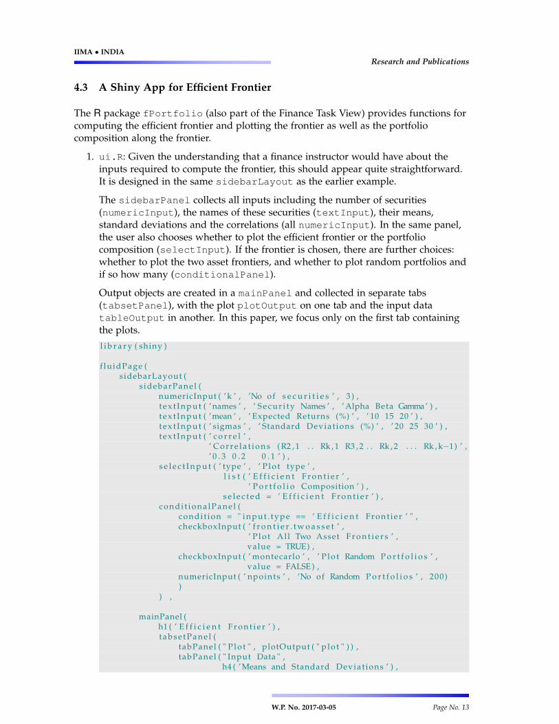
The R package fPortfolio (also part of the Finance Task View) provides functions forcomputing the efficient frontier and plotting the frontier as well as the portfoliocomposition along the frontier.

1. ui.R: Given the understanding that a finance instructor would have about theinputs required to compute the frontier, this should appear quite straightforward.It is designed in the same sidebarLayout as the earlier example.

The sidebarPanel collects all inputs including the number of securities(numericInput), the names of these securities (textInput), their means,standard deviations and the correlations (all numericInput). In the same panel,the user also chooses whether to plot the efficient frontier or the portfoliocomposition (selectInput). If the frontier is chosen, there are further choices:whether to plot the two asset frontiers, and whether to plot random portfolios andif so how many (conditionalPanel).

Output objects are created in a mainPanel and collected in separate tabs(tabsetPanel), with the plot plotOutput on one tab and the input datatableOutput in another. In this paper, we focus only on the first tab containingthe plots.

l i b r a r y ( shiny )

f luidPage (sidebarLayout (

s idebarPanel (numericInput ( ’ k ’ , ’No of s e c u r i t i e s ’ , 3 ) ,t e x t I n p u t ( ’ names ’ , ’ S e c u r i t y Names ’ , ’ Alpha Beta Gamma ’ ) ,t e x t I n p u t ( ’mean ’ , ’ Expected Returns (%) ’ , ’ 10 15 20 ’ ) ,t e x t I n p u t ( ’ sigmas ’ , ’ Standard Deviat ions (%) ’ , ’ 20 25 30 ’ ) ,t e x t I n p u t ( ’ c o r r e l ’ ,

’ C o r r e l a t i o n s ( R2 , 1 . . Rk , 1 R3 , 2 . . Rk , 2 . . . Rk , k−1) ’ ,’ 0 . 3 0 . 2 0 . 1 ’ ) ,

s e l e c t I n p u t ( ’ type ’ , ’ P l o t type ’ ,l i s t ( ’ E f f i c i e n t F r o n t i e r ’ ,

’ P o r t f o l i o Composition ’ ) ,s e l e c t e d = ’ E f f i c i e n t F r o n t i e r ’ ) ,

c on di t i on a l Pa ne l (condi t ion = " i n p u t . t y p e == ’ E f f i c i e n t Front ie r ’ " ,checkboxInput ( ’ f r o n t i e r . t w o a s s e t ’ ,

’ P l o t Al l Two Asset F r o n t i e r s ’ ,value = TRUE) ,

checkboxInput ( ’ montecarlo ’ , ’ P l o t Random P o r t f o l i o s ’ ,value = FALSE ) ,

numericInput ( ’ npoints ’ , ’No of Random P o r t f o l i o s ’ , 200))

) ,

mainPanel (h1 ( ’ E f f i c i e n t F r o n t i e r ’ ) ,t a b s e t P a n e l (

tabPanel ( " P l o t " , plotOutput ( " p l o t " ) ) ,tabPanel ( " Input Data " ,

h4 ( ’Means and Standard Deviat ions ’ ) ,

W.P. No. 2017-03-05 Page No. 13

IIMA • INDIAResearch and Publications

tableOutput ( " mu.sd " ) ,h4 ( ’ C o r r e l a t i o n Matrix ’ ) ,tableOutput ( " rho " ))

))

) ,t i t l e =" E f f i c i e n t F r o n t i e r "

)

2. server.R: The server script requires a bit more work. It needs to read the inputs,compute the correlation matrix and render the output. That said, the reactivitypart of the code remains simple as in the case of the histogram. It calls thefollowing functions from fPortfolio:

• portfolioFrontier computes the frontier, and weightsPlot plots theportfolio composition (weights)

• twoAssetsLines plots all two-asset efficient frontiers. If there are threesecurities, A, B and C, the efficient frontier drawn by portfolioFrontiercontains portfolios including all three stocks. twoAssetsLines draws threeadditional efficient frontiers taking two securities at a time: the frontiers withonly A and B, with only A and C and with only B and C.

• monteCarloPoints plots the mean and standard deviation of a number ofrandom portfolios. Most of these would be inefficient portfolios, but they mapout the entire feasible region in mean – standard deviation space. The efficientfrontier produced by portfolioFrontier appears as the upper boundaryof the feasible region.

my.sample() part of the code is explained later. It is there because of a quirk inthe way fPortfolio package uses sample moments.

l i b r a r y ( shiny )l i b r a r y ( f P o r t f o l i o )

funct ion ( input , output ) {## Code to read inputs and generate sample is omitted ...## ... and is implemented before renderPlot({...}) here ...## ...output $ p l o t ← renderPlot ( {

fp ← p o r t f o l i o F r o n t i e r ( a s . t i m e S e r i e s ( my.sample ( ) ) )i f ( input $ type == ’ P o r t f o l i o Composition ’ ) {

weightsPlot ( fp )} e l s e {

f r o n t i e r P l o t ( fp , c o l = c ( ’ blue ’ , ’ red ’ ) , pch = 20)i f ( input $ f r o n t i e r . t w o a s s e t )

twoAssetsLines ( fp , c o l = ’ green ’ )i f ( input $ montecarlo )

monteCarloPoints ( fp , input $ npoints ,c o l = ’ grey ’ , pch = 20 , cex=0 . 3 )

}} )

}

W.P. No. 2017-03-05 Page No. 14

IIMA • INDIAResearch and Publications

3. Preparation work in server.R: The remaining part of the server script (beforerenderPlot) consists in parsing the input data, and computing correlations. Inthis particular case, the mean input also needs to be converted from percent todecimal:27

mu ← r e a c t i v e ( scan ( t e x t =input $mean , quie t = TRUE) / 100)

Note that while the scan function is standard in R for reading text data, reactivityrequires that this be called as a reactive expression so that it can respond to anychanges in the data input by the user.

The correlation matrix computation part of the code (not reproduced here) takes alittle more effort because only the lower triangular part of the correlation matrix istyped by the user, and the code has to copy this into the upper triangular part andalso fill the diagonal with ones. This requires about a dozen lines of R code easilyunderstood by anyone with a basic understanding of correlation matrix. The fullsource code is available on the first author’s Github page.28

4. my.sample() object in server.R: There is a quirk in the fPortfolio packagein that it does not allow direct input of mean and covariances, but insists oncomputing these from a time series of returns. We have no choice but to generatean appropriate sample of returns and feed these returns to the package.

Now, R has no difficulty generating a sample with specified population meanvector and variance-covariance matrix. The problem is that the sample mean andvariance of this sample will not be exactly equal to that of the populationparameters. One option is to choose a large sample and ignore the smalldifferences between the sample and population values.

This is one of the things that can often get ‘hand-waved’ when using spreadsheetsin the class. In R there is no such problem. With a bit of re-centering and re-scaling,one can ensure that the sample means and covariances are exactly equal to thedesired population values. A non-programmer audience needn’t worry about allthis, but when they input a desired population moment that is what gets used.

One could argue that it is the use of the fPortfolio package that causes theproblem so one should avoid it. But it is one of the most reliable and widely usedpackages for portfolio analysis in the R universe. And given that the source code iscompletely transparent about its methods, it is easier to deal with any issue thanworking with a black-box.

After the iid.sample() code draws uncorrelated multivariate normal variates,and forces the mean to 0, standard deviation to 1 and removes sample correlation,the server script deals with scaling of means, variance and correlation as follows:

• Means and variances: R provides a function scale that can be used torecenter and rescale a sample to change the univariate means and variances.One can also do this directly by dividing the data with sample standarddeviation and multiplying the resulting new series by the populationstandard deviation.

27Input format and its use in the code is something that needs to be kept in mind during development.28https://github.com/jrvarma

W.P. No. 2017-03-05 Page No. 15

IIMA • INDIAResearch and Publications

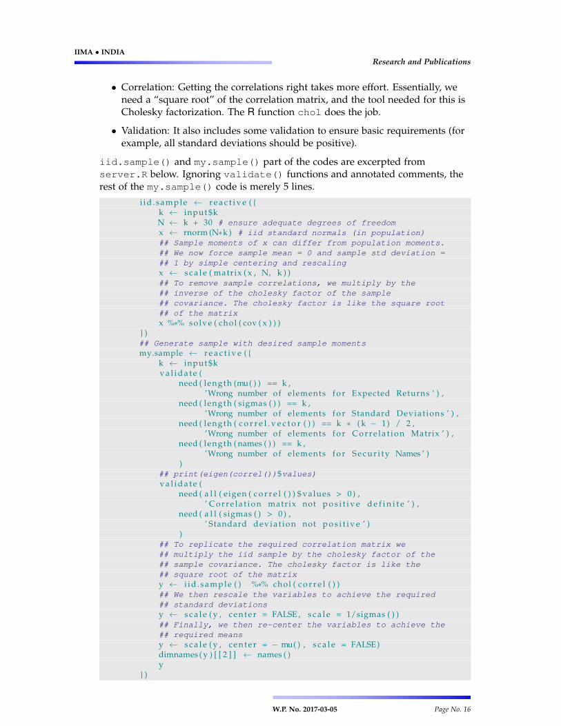
• Correlation: Getting the correlations right takes more effort. Essentially, weneed a “square root” of the correlation matrix, and the tool needed for this isCholesky factorization. The R function chol does the job.

• Validation: It also includes some validation to ensure basic requirements (forexample, all standard deviations should be positive).

iid.sample() and my.sample() part of the codes are excerpted fromserver.R below. Ignoring validate() functions and annotated comments, therest of the my.sample() code is merely 5 lines.

i i d . s am ple ← r e a c t i v e ( {k ← input $kN ← k + 30 # ensure adequate degrees of freedomx ← rnorm (N∗k ) # iid standard normals (in population)## Sample moments of x can differ from population moments.## We now force sample mean = 0 and sample std deviation =## 1 by simple centering and rescalingx ← s c a l e ( matrix ( x , N, k ) )## To remove sample correlations, we multiply by the## inverse of the cholesky factor of the sample## covariance. The cholesky factor is like the square root## of the matrixx %∗% solve ( chol ( cov ( x ) ) )

} )## Generate sample with desired sample momentsmy.sample ← r e a c t i v e ( {

k ← input $kv a l i d a t e (

need ( length (mu( ) ) == k ,’Wrong number of elements f o r Expected Returns ’ ) ,

need ( length ( sigmas ( ) ) == k ,’Wrong number of elements f o r Standard Deviat ions ’ ) ,

need ( length ( c o r r e l . v e c t o r ( ) ) == k ∗ ( k − 1) / 2 ,’Wrong number of elements f o r C o r r e l a t i o n Matrix ’ ) ,

need ( length ( names ( ) ) == k ,’Wrong number of elements f o r S e c u r i t y Names ’ )

)## print(eigen(correl())$values)v a l i d a t e (

need ( a l l ( eigen ( c o r r e l ( ) ) $ values > 0 ) ,’ C o r r e l a t i o n matrix not p o s i t i v e d e f i n i t e ’ ) ,

need ( a l l ( sigmas ( ) > 0 ) ,’ Standard devia t ion not p o s i t i v e ’ )

)## To replicate the required correlation matrix we## multiply the iid sample by the cholesky factor of the## sample covariance. The cholesky factor is like the## square root of the matrixy ← i i d . s am ple ( ) %∗% chol ( c o r r e l ( ) )## We then rescale the variables to achieve the required## standard deviationsy ← s c a l e ( y , c e n t e r = FALSE , s c a l e = 1/sigmas ( ) )## Finally, we then re-center the variables to achieve the## required meansy ← s c a l e ( y , c e n t e r = − mu( ) , s c a l e = FALSE)dimnames ( y ) [ [ 2 ] ] ← names ( )y

} )

W.P. No. 2017-03-05 Page No. 16

IIMA • INDIAResearch and Publications

4.4 Shiny-R Advantages for Finance

While prima-facie the steps involved in building Shiny apps may seem intimidating, aninstructor who needs to use or build similar applications regularly for teaching orresearch the benefits far outweigh the cost in our opinion.

Reusability. Once the apps are created, they can be used across for different audiencethat one encounters in a business school. While this is shared with Excel forsimple/toy examples to an extent, as argued earlier, Shiny keeps the focus on theelements crucial for a session. The layout of the app can be designed such that thesame app can be used for different groups by using tabs to separate differentoutputs by difficulty level. Select data can also be made non-reactive by usingisolate() as need be.

Object-oriented and vectorized. Many problems in asset pricing and investmentanalysis are naturally cast in terms of linear algebra. This makes R analmost-perfect fit for the task, given that indexing, operators and functions in Rclosely resemble the algebra of matrices. Its vectorization capabilities are oftenleveraged to speed up the code (Wang et al., 2015).

Graphics. Spreadsheets are particularly infamous for the poor quality of their chartingutility for communicating scientific results. In comparison, R offers a modernapproach to data visualization using the layered grammar of graphics with apackage called ggplot2 (Wickham, 2010). Coupled with the interactivity thatShiny offers, ggplot2 is leaps ahead of any spreadsheet software in exploring andvisualizing complex data.

Extensions The biggest advantage of working in the R and Shiny environment ispossibilities afforded for extensions to the server script by including moreadvanced versions of basic models. Some possible extensions include:

• Non-Normality of asset returns, say, by bringing in other elliptical or stabledistribution using, for example, the fBasics package

• Black-Litterman’s approach (Black and Litterman, 1992) for introducinginvestor views and opinions in the Markowitz problem using the BLCOPpackage. For many such nonlinear problems, spreadsheets are known to beparticularly unsuitable (Almiron et al., 2010)

• Bring in stylized facts (Cont, 2001) and time series methods to the class usingfGarch, rugarch and rmgarch packages.

• Bring in live financial and macroeconomic data from important financialmarkets directly into the R workspace using packages like quantMod andquandl.

• Animate apps as GIF or flash movie using the animate package (Xie, 2013)

These are only a few obvious examples. Richness of R allows for customization andextensions in different directions.

Of course, the context decides, but depending on the audience, the apps can be as basicor as sophisticated as need be. While investment required on part of the instructor

W.P. No. 2017-03-05 Page No. 17

IIMA • INDIAResearch and Publications

differs depending on the nature of the app, the user experience at all difficulty levelsremains the same. All Shiny apps essentially involve interacting with the browser,however simple or complex the app may be. It’s a bit like an Android smart phone. Ahigh-end Android phone may have more features (so costs more) than a low-end one,but both run on the same kernel and offer the same basic functionality.

5 Sharing and Deploying Shiny Apps

5.1 Sharing the component files

If the users are familiar with R and have all the necessary data available and R packagesare installed on their computers, sharing a Shiny app is as easy sharing the componentfiles and instructions to run the app. It is crude, but it works and may work for a smallclass.

This may not be ideal with a non-programmer audience though, as the users mayinadvertently damage the app by tinkering with the user interface or server files. If theobjective, however, is to teach R and Shiny, then an instructor could share componentfiles for an incomplete app and have students finish them as homework. Other thansimply sharing the two files over a network or otherwise, they can also be hosted onGithub or Gist and run directly from there.29

5.2 Hosting a Shiny server

If the users do not have R installed or are not keen to, the utility of Shiny really comesthrough as an app hosted on cloud. All the users need is a browser and instructions forrunning the app.

RStudio provides a paid service to do so at https://www.shinyapps.io/. They alsohave a basic free/trial version. An alternative to using RStudio is to deploy apps using aDocker-based technology30 at the service called ShinyProxy which only relies on theopen-source Shiny package without any dependency on the server version of Shiny orRStudio.31

Those with some experience in web hosting or a helpful IT department may either set upa Shiny server locally32 or on any cloud hosting service, be it, e.g., Amazon EC2, GoogleCloud or Digital Ocean.33

Given the popularity of free Amazon EC2, in Appendix A we provide steps to install andrun the efficient frontier Shiny app discussed earlier on Amazon Web Services (AWS).

29https://shiny.rstudio.com/articles/deployment-local.html, accessed March 27, 2017.30https://www.docker.com/31More details at https://www.shinyproxy.io/32https://github.com/rstudio/shiny-server/33For an example, see http://deanattali.com/2015/05/09/setup-rstudio-shiny-server-

digital-ocean/, accessed March 27, 2017.

W.P. No. 2017-03-05 Page No. 18

IIMA • INDIAResearch and Publications

6 Conclusion

As the data science and analytics industry has grown, so has the popularity ofopen-source languages like Python and R . While the former has gained in importancedue to its versatility, R has fast grown into one of the most popular languages forempirical research in social science. There are not many competitors for R when itcomes to applications in statistical computing in practice.

For beginning data analysis courses at business schools, however, the software of choiceremains Microsoft Excel despite the known problems for its usage in serious finance andstatistics applications. It’s not merely inertia, but a combination low barriers to entryand lack of exposure of business school students to programming. Even if instructorsare adept at using R , they are forced to use Excel given its popularity. The nature ofspreadsheets often significantly constrains the depth of analysis possible in the class,often even requiring dumbing-down of the subject.

Recent software advances have brought browser-based tools to fore as capablealternatives to spreadsheets. In this article we have introduced one such tool calledShiny. Since a Shiny app is essentially an HTML document hosted on a computerrunning R , it is able to leverage the power of HTML and CSS with the sophistication ofthe R programming language. Once developed, the apps can be shared via cloud andrun on any browser-enabled device, making it ideal for teaching. With the detaileddocumentation available for both R and Shiny, an interested instructor can get up tospeed in quick time.

After describing the design philosophy of Shiny and elements of a Shiny app with a toyexample, we have provided detailed steps for building an app for explainingmean-variance efficient frontier with arbitrary number of securities. The app is not onlyamenable to extensions for more advanced courses, it is also straightforward to set it upon the cloud for easy accessibility by any modern browser.

W.P. No. 2017-03-05 Page No. 19

IIMA • INDIAResearch and Publications

References

Adams, W. C., Infeld, D. L., and Wulff, C. M. (2013). Statistical software for curriculumand careers. Journal of Public Affairs Education, 19(1):173–188.

Almiron, M., Lopes, B., Oliveira, A., Medeiros, A., and Frery, A. (2010). On thenumerical accuracy of spreadsheets. Journal of Statistical Software, 34(1):1–29.

Bank of International Settlements (2013). Principles for effective risk data aggregationand risk reporting. Technical report, Bank of International Settlements.

Barreto, H. (2015). Why Excel? The Journal of Economic Education, 46(3):300–309.

Berenson, M. L. (2013). Using Excel for White’s Test - An Important Technique forEvaluating the Equality of Variance Assumption and Model Specification in aRegression Analysis. Decision Sciences Journal of Innovative Education, 11(3):243–262.

Black, F. and Litterman, R. (1992). Global portfolio optimization. Financial AnalystsJournal, 48(5):28–43.

Cont, R. (2001). Empirical properties of asset returns: stylized facts and statistical issues.Quantitative Finance, 1(2):223–236.

JP Morgan (2013). Report of JPMorgan Chase & Co. Management Task Force Regarding2012 CIO Losses.http://files.shareholder.com/downloads/ONE/2272984969x0x628656/4cb574a0-0bf5-4728-9582-625e4519b5ab/Task_Force_Report.pdf.Accessed March 27, 2017.

Markowitz, H. (1952). Portfolio selection. The Journal of Finance, 7(1):77–91.

McCullough, B. and Heiser, D. A. (2008). On the accuracy of statistical procedures inMicrosoft Excel 2007. Computational Statistics & Data Analysis, 52(10):4570 – 4578.

McDermott, J. (2010). Returns-Based Style Analysis: An Excel-Based Classroom Exercise.Journal of Education for Business, 85:107–113.

Merton, R. C. (1972). An analytic derivation of the efficient portfolio frontier. The Journalof Financial and Quantitative Analysis, 7(4):1851–1872.

Nash, J. C. (2006). Spreadsheets in statistical practice—another look. The AmericanStatistician, 60(3):287–289.

Nævdal, E. (2003). Solving Continuous-Time Optimal-Control Problems with aSpreadsheet. The Journal of Economic Education, 34(2):99–122.

Panko, R. R. and Ordway, N. (2008). Sarbanes-oxley: What about all the spreadsheets?arXiv:0804.0797 [cs.SE], abs/0804.0797.

Wang, H., Padua, D., and Wu, P. (2015). Vectorization of apply to reduce interpretationoverhead of r. SIGPLAN Not., 50(10):400–415.

Wickham, H. (2010). A Layered Grammar of Graphics. Journal of Computational andGraphical Statistics, 19(1):3–28.

W.P. No. 2017-03-05 Page No. 20

IIMA • INDIAResearch and Publications

Xie, Y. (2013). animation: An r package for creating animations and demonstratingstatistical methods. Journal of Statistical Software, 53(1):1–27.

Yalta, A. T. (2008). The accuracy of statistical distributions in Microsoft Excel 2007.Computational Statistics & Data Analysis, 52(10):4579 – 4586.

Zeileis, A. (2005). CRAN Task Views. R News, 5(1):39–40.

Zhang, C. (2015). Incorporating Powerful Excel Tools into Finance Teaching. Journal ofFinancial Education, 40:87–113.

W.P. No. 2017-03-05 Page No. 21

IIMA • INDIAResearch and Publications

A Deploying the Efficient Frontier Shiny App on Amazon WebServices

The following steps sets up the efficient frontier Shiny app on a Free Tier EC2 instanceon Amazon Web Services (AWS).

A.1 Creating the instance

The basic setup takes only a couple of minutes:

• Create an Amazon account (or use an existing account)

• Log into the AWS console https://console.aws.amazon.com/

• Launch an EC2 Instance: choose the Ubuntu Server 16.04 LTS AmazonMachine Image (AMI), select a t2.micro instance type

• Create new key pair, download it as say my-key.pem and change the filepermissions to give all rights only to the owner (Unix permission 400).

• From the AWS Console, determine the public DNS (hostname) of the instance saymy-ec2.amazonaws.com

To connect to a running instance one needs to use secure shell (SSH) as:

ssh -i my-key.pem ubuntu@my-ec2.amazonaws.com

A.2 Installing R on the instance

We then proceed to install R and all requisite packages to install the fPortfolio Rpackage:

# Some p a c k a g e s r e q u i r e newer v e r s i o n o f R , so we use t h e RStudior e p o s i t o r y

sudo apt−key adv −−keyserver keyserver . ubuntu . com −−recv−keysE298A3A825C0D65DFD57CBB651716619E084DAB9

sudo add−apt−r e p o s i t o r y ’ deb [ arch=amd64 , i386 ] ht tps : / / cran .r s t ud io . com / bin / l inux / ubuntu x e n i a l / ’

sudo apt−get updatesudo apt−get upgradesudo apt−get i n s t a l l r−base# i n s t a l l a l l p a c k a g e s r e q u i r e d f o r f P o r t f o l i o and i t s

d e p e n d e n c i e ssudo apt−get i n s t a l l l i b c u r l 4−openssl−devsudo apt−get i n s t a l l l ibxml2−devsudo apt−get i n s t a l l coinor−symphony coinor−libsymphony−dev

coinor−l i b c g l−devsudo apt−get i n s t a l l xorg−dev l ibg lu1−mesa−devsudo apt−get i n s t a l l glpk−u t i l s l ibg lpk−dev

W.P. No. 2017-03-05 Page No. 22

IIMA • INDIAResearch and Publications

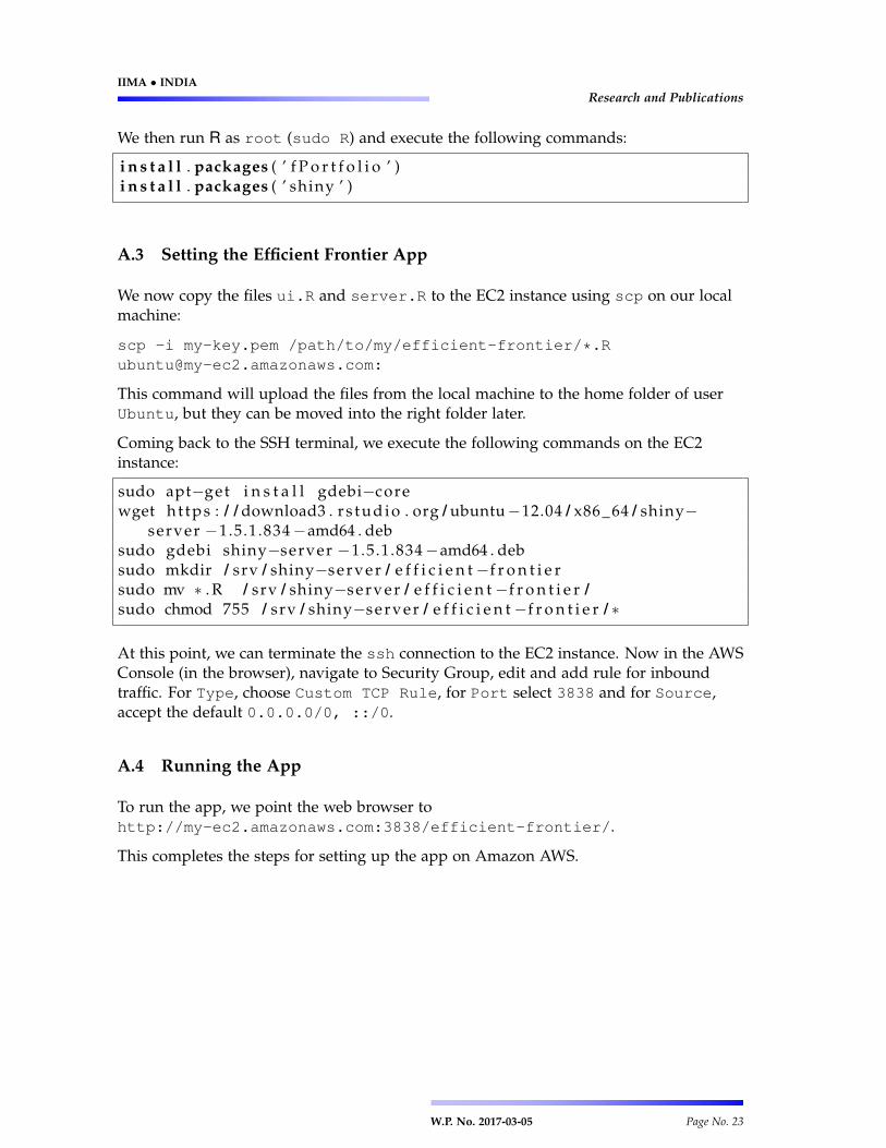
We then run R as root (sudo R) and execute the following commands:

i n s t a l l . packages ( ’ f P o r t f o l i o ’ )i n s t a l l . packages ( ’ shiny ’ )

A.3 Setting the Efficient Frontier App

We now copy the files ui.R and server.R to the EC2 instance using scp on our localmachine:

scp -i my-key.pem /path/to/my/efficient-frontier/*.Rubuntu@my-ec2.amazonaws.com:

This command will upload the files from the local machine to the home folder of userUbuntu, but they can be moved into the right folder later.

Coming back to the SSH terminal, we execute the following commands on the EC2instance:

sudo apt−get i n s t a l l gdebi−corewget ht tps : / / download3 . r s tu di o . org / ubuntu−12.04 / x86_64 / shiny−

server −1.5.1.834−amd64 . debsudo gdebi shiny−server −1.5.1.834−amd64 . debsudo mkdir / srv / shiny−server / e f f i c i e n t−f r o n t i e rsudo mv ∗ . R / srv / shiny−server / e f f i c i e n t−f r o n t i e r /sudo chmod 755 / srv / shiny−server / e f f i c i e n t−f r o n t i e r / ∗

At this point, we can terminate the ssh connection to the EC2 instance. Now in the AWSConsole (in the browser), navigate to Security Group, edit and add rule for inboundtraffic. For Type, choose Custom TCP Rule, for Port select 3838 and for Source,accept the default 0.0.0.0/0, ::/0.

A.4 Running the App

To run the app, we point the web browser tohttp://my-ec2.amazonaws.com:3838/efficient-frontier/.

This completes the steps for setting up the app on Amazon AWS.

W.P. No. 2017-03-05 Page No. 23