Shigley's Mechanical Engineering - AnalysisChamp.com · design, turbomachinery design, and...
137
Budynas-Nisbett: Shigley’s Mechanical Engineering Design, Eighth Edition I. Basics Introduction 8 © The McGraw-Hill Companies, 2008 PART 1 Basics
Transcript of Shigley's Mechanical Engineering - AnalysisChamp.com · design, turbomachinery design, and...

Budynas−Nisbett: Shigley’s
Mechanical Engineering
Design, Eighth Edition
I. Basics Introduction8 © The McGraw−Hill
Companies, 2008
PART1Basics

Budynas−Nisbett: Shigley’s
Mechanical Engineering
Design, Eighth Edition
I. Basics 1. Introduction to
Mechanical Engineering
Design
9© The McGraw−Hill
Companies, 2008
3
Chapter Outline
1–1 Design 4
1–2 Mechanical Engineering Design 5
1–3 Phases and Interactions of the Design Process 5
1–4 Design Tools and Resources 8
1–5 The Design Engineer’s Professional Responsibilities 10
1–6 Standards and Codes 12
1–7 Economics 12
1–8 Safety and Product Liability 15
1–9 Stress and Strength 15
1–10 Uncertainty 16
1–11 Design Factor and Factor of Safety 17
1–12 Reliability 18
1–13 Dimensions and Tolerances 19
1–14 Units 21
1–15 Calculations and Significant Figures 22
1–16 Power Transmission Case Study Specifications 23
1Introduction to MechanicalEngineering Design

Budynas−Nisbett: Shigley’s
Mechanical Engineering
Design, Eighth Edition
I. Basics 1. Introduction to
Mechanical Engineering
Design
10 © The McGraw−Hill
Companies, 2008
4 Mechanical Engineering Design
Mechanical design is a complex undertaking, requiring many skills. Extensive relation-
ships need to be subdivided into a series of simple tasks. The complexity of the subject
requires a sequence in which ideas are introduced and iterated.
We first address the nature of design in general, and then mechanical engineering
design in particular. Design is an iterative process with many interactive phases. Many
resources exist to support the designer, including many sources of information and an
abundance of computational design tools. The design engineer needs not only to develop
competence in their field but must also cultivate a strong sense of responsibility and
professional work ethic.
There are roles to be played by codes and standards, ever-present economics, safety,
and considerations of product liability. The survival of a mechanical component is often
related through stress and strength. Matters of uncertainty are ever-present in engineer-
ing design and are typically addressed by the design factor and factor of safety, either
in the form of a deterministic (absolute) or statistical sense. The latter, statistical
approach, deals with a design’s reliability and requires good statistical data.
In mechanical design, other considerations include dimensions and tolerances,
units, and calculations.
The book consists of four parts. Part 1, Basics, begins by explaining some differ-
ences between design and analysis and introducing some fundamental notions and
approaches to design. It continues with three chapters reviewing material properties,
stress analysis, and stiffness and deflection analysis, which are the key principles nec-
essary for the remainder of the book.
Part 2, Failure Prevention, consists of two chapters on the prevention of failure of
mechanical parts. Why machine parts fail and how they can be designed to prevent fail-
ure are difficult questions, and so we take two chapters to answer them, one on pre-
venting failure due to static loads, and the other on preventing fatigue failure due to
time-varying, cyclic loads.
In Part 3, Design of Mechanical Elements, the material of Parts 1 and 2 is applied
to the analysis, selection, and design of specific mechanical elements such as shafts,
fasteners, weldments, springs, rolling contact bearings, film bearings, gears, belts,
chains, and wire ropes.
Part 4, Analysis Tools, provides introductions to two important methods used in
mechanical design, finite element analysis and statistical analysis. This is optional study
material, but some sections and examples in Parts 1 to 3 demonstrate the use of these tools.
There are two appendixes at the end of the book. Appendix A contains many use-
ful tables referenced throughout the book. Appendix B contains answers to selected
end-of-chapter problems.
1–1 DesignTo design is either to formulate a plan for the satisfaction of a specified need or to solve
a problem. If the plan results in the creation of something having a physical reality, then
the product must be functional, safe, reliable, competitive, usable, manufacturable, and
marketable.
Design is an innovative and highly iterative process. It is also a decision-making
process. Decisions sometimes have to be made with too little information, occasion-
ally with just the right amount of information, or with an excess of partially contradictory
information. Decisions are sometimes made tentatively, with the right reserved to adjust
as more becomes known. The point is that the engineering designer has to be personally
comfortable with a decision-making, problem-solving role.

Budynas−Nisbett: Shigley’s
Mechanical Engineering
Design, Eighth Edition
I. Basics 1. Introduction to
Mechanical Engineering
Design
11© The McGraw−Hill
Companies, 2008
Introduction to Mechanical Engineering Design 5
Design is a communication-intensive activity in which both words and pictures are
used, and written and oral forms are employed. Engineers have to communicate effec-
tively and work with people of many disciplines. These are important skills, and an
engineer’s success depends on them.
A designer’s personal resources of creativeness, communicative ability, and problem-
solving skill are intertwined with knowledge of technology and first principles.
Engineering tools (such as mathematics, statistics, computers, graphics, and languages)
are combined to produce a plan that, when carried out, produces a product that is func-
tional, safe, reliable, competitive, usable, manufacturable, and marketable, regardless
of who builds it or who uses it.
1–2 Mechanical Engineering DesignMechanical engineers are associated with the production and processing of energy and
with providing the means of production, the tools of transportation, and the techniques
of automation. The skill and knowledge base are extensive. Among the disciplinary
bases are mechanics of solids and fluids, mass and momentum transport, manufactur-
ing processes, and electrical and information theory. Mechanical engineering design
involves all the disciplines of mechanical engineering.
Real problems resist compartmentalization. A simple journal bearing involves fluid
flow, heat transfer, friction, energy transport, material selection, thermomechanical
treatments, statistical descriptions, and so on. A building is environmentally controlled.
The heating, ventilation, and air-conditioning considerations are sufficiently specialized
that some speak of heating, ventilating, and air-conditioning design as if it is separate
and distinct from mechanical engineering design. Similarly, internal-combustion engine
design, turbomachinery design, and jet-engine design are sometimes considered dis-
crete entities. Here, the leading string of words preceding the word design is merely a
product descriptor. Similarly, there are phrases such as machine design, machine-element
design, machine-component design, systems design, and fluid-power design. All of
these phrases are somewhat more focused examples of mechanical engineering design.
They all draw on the same bodies of knowledge, are similarly organized, and require
similar skills.
1–3 Phases and Interactions of the Design ProcessWhat is the design process? How does it begin? Does the engineer simply sit down at
a desk with a blank sheet of paper and jot down some ideas? What happens next? What
factors influence or control the decisions that have to be made? Finally, how does the
design process end?
The complete design process, from start to finish, is often outlined as in Fig. 1–1.
The process begins with an identification of a need and a decision to do something
about it. After many iterations, the process ends with the presentation of the plans
for satisfying the need. Depending on the nature of the design task, several design
phases may be repeated throughout the life of the product, from inception to termi-
nation. In the next several subsections, we shall examine these steps in the design
process in detail.
Identification of need generally starts the design process. Recognition of the need
and phrasing the need often constitute a highly creative act, because the need may be
only a vague discontent, a feeling of uneasiness, or a sensing that something is not right.
The need is often not evident at all; recognition is usually triggered by a particular

Budynas−Nisbett: Shigley’s
Mechanical Engineering
Design, Eighth Edition
I. Basics 1. Introduction to
Mechanical Engineering
Design
12 © The McGraw−Hill
Companies, 2008
6 Mechanical Engineering Design
adverse circumstance or a set of random circumstances that arises almost simultaneously.
For example, the need to do something about a food-packaging machine may be indi-
cated by the noise level, by a variation in package weight, and by slight but perceptible
variations in the quality of the packaging or wrap.
There is a distinct difference between the statement of the need and the definition
of the problem. The definition of problem is more specific and must include all the spec-
ifications for the object that is to be designed. The specifications are the input and out-
put quantities, the characteristics and dimensions of the space the object must occupy,
and all the limitations on these quantities. We can regard the object to be designed as
something in a black box. In this case we must specify the inputs and outputs of the box,
together with their characteristics and limitations. The specifications define the cost, the
number to be manufactured, the expected life, the range, the operating temperature, and
the reliability. Specified characteristics can include the speeds, feeds, temperature lim-
itations, maximum range, expected variations in the variables, dimensional and weight
limitations, etc.
There are many implied specifications that result either from the designer’s par-
ticular environment or from the nature of the problem itself. The manufacturing
processes that are available, together with the facilities of a certain plant, constitute
restrictions on a designer’s freedom, and hence are a part of the implied specifica-
tions. It may be that a small plant, for instance, does not own cold-working machin-
ery. Knowing this, the designer might select other metal-processing methods that
can be performed in the plant. The labor skills available and the competitive situa-
tion also constitute implied constraints. Anything that limits the designer’s freedom
of choice is a constraint. Many materials and sizes are listed in supplier’s catalogs,
for instance, but these are not all easily available and shortages frequently occur.
Furthermore, inventory economics requires that a manufacturer stock a minimum
number of materials and sizes. An example of a specification is given in Sec. 1–16.
This example is for a case study of a power transmission that is presented throughout
this text.
The synthesis of a scheme connecting possible system elements is sometimes
called the invention of the concept or concept design. This is the first and most impor-
tant step in the synthesis task. Various schemes must be proposed, investigated, and
Figure 1–1
The phases in design,acknowledging the manyfeedbacks and iterations.
Identification of need
Definition of problem
Synthesis
Analysis and optimization
Evaluation
Presentation
Iteration

Budynas−Nisbett: Shigley’s
Mechanical Engineering
Design, Eighth Edition
I. Basics 1. Introduction to
Mechanical Engineering
Design
13© The McGraw−Hill
Companies, 2008
Introduction to Mechanical Engineering Design 7
quantified in terms of established metrics.1 As the fleshing out of the scheme progresses,
analyses must be performed to assess whether the system performance is satisfactory or
better, and, if satisfactory, just how well it will perform. System schemes that do not
survive analysis are revised, improved, or discarded. Those with potential are optimized
to determine the best performance of which the scheme is capable. Competing schemes
are compared so that the path leading to the most competitive product can be chosen.
Figure 1–1 shows that synthesis and analysis and optimization are intimately and
iteratively related.
We have noted, and we emphasize, that design is an iterative process in which we
proceed through several steps, evaluate the results, and then return to an earlier phase
of the procedure. Thus, we may synthesize several components of a system, analyze and
optimize them, and return to synthesis to see what effect this has on the remaining parts
of the system. For example, the design of a system to transmit power requires attention
to the design and selection of individual components (e.g., gears, bearings, shaft).
However, as is often the case in design, these components are not independent. In order
to design the shaft for stress and deflection, it is necessary to know the applied forces.
If the forces are transmitted through gears, it is necessary to know the gear specifica-
tions in order to determine the forces that will be transmitted to the shaft. But stock
gears come with certain bore sizes, requiring knowledge of the necessary shaft diame-
ter. Clearly, rough estimates will need to be made in order to proceed through the
process, refining and iterating until a final design is obtained that is satisfactory for each
individual component as well as for the overall design specifications. Throughout the
text we will elaborate on this process for the case study of a power transmission design.
Both analysis and optimization require that we construct or devise abstract models
of the system that will admit some form of mathematical analysis. We call these mod-
els mathematical models. In creating them it is our hope that we can find one that will
simulate the real physical system very well. As indicated in Fig. 1–1, evaluation is a
significant phase of the total design process. Evaluation is the final proof of a success-
ful design and usually involves the testing of a prototype in the laboratory. Here we
wish to discover if the design really satisfies the needs. Is it reliable? Will it compete
successfully with similar products? Is it economical to manufacture and to use? Is it
easily maintained and adjusted? Can a profit be made from its sale or use? How likely
is it to result in product-liability lawsuits? And is insurance easily and cheaply
obtained? Is it likely that recalls will be needed to replace defective parts or systems?
Communicating the design to others is the final, vital presentation step in the
design process. Undoubtedly, many great designs, inventions, and creative works have
been lost to posterity simply because the originators were unable or unwilling to
explain their accomplishments to others. Presentation is a selling job. The engineer,
when presenting a new solution to administrative, management, or supervisory persons,
is attempting to sell or to prove to them that this solution is a better one. Unless this can
be done successfully, the time and effort spent on obtaining the solution have been
largely wasted. When designers sell a new idea, they also sell themselves. If they are
repeatedly successful in selling ideas, designs, and new solutions to management, they
begin to receive salary increases and promotions; in fact, this is how anyone succeeds
in his or her profession.
1An excellent reference for this topic is presented by Stuart Pugh, Total Design—Integrated Methods for
Successful Product Engineering, Addison-Wesley, 1991. A description of the Pugh method is also provided
in Chap. 8, David G. Ullman, The Mechanical Design Process, 3rd ed., McGraw-Hill, 2003.

Budynas−Nisbett: Shigley’s
Mechanical Engineering
Design, Eighth Edition
I. Basics 1. Introduction to
Mechanical Engineering
Design
14 © The McGraw−Hill
Companies, 2008
8 Mechanical Engineering Design
Design Considerations
Sometimes the strength required of an element in a system is an important factor in the
determination of the geometry and the dimensions of the element. In such a situation
we say that strength is an important design consideration. When we use the expression
design consideration, we are referring to some characteristic that influences the design
of the element or, perhaps, the entire system. Usually quite a number of such charac-
teristics must be considered and prioritized in a given design situation. Many of the
important ones are as follows (not necessarily in order of importance):
1 Functionality 14 Noise
2 Strength/stress 15 Styling
3 Distortion/deflection/stiffness 16 Shape
4 Wear 17 Size
5 Corrosion 18 Control
6 Safety 19 Thermal properties
7 Reliability 20 Surface
8 Manufacturability 21 Lubrication
9 Utility 22 Marketability
10 Cost 23 Maintenance
11 Friction 24 Volume
12 Weight 25 Liability
13 Life 26 Remanufacturing/resource recovery
Some of these characteristics have to do directly with the dimensions, the material, the
processing, and the joining of the elements of the system. Several characteristics may
be interrelated, which affects the configuration of the total system.
1–4 Design Tools and ResourcesToday, the engineer has a great variety of tools and resources available to assist in the
solution of design problems. Inexpensive microcomputers and robust computer soft-
ware packages provide tools of immense capability for the design, analysis, and simu-
lation of mechanical components. In addition to these tools, the engineer always needs
technical information, either in the form of basic science/engineering behavior or the
characteristics of specific off-the-shelf components. Here, the resources can range from
science/engineering textbooks to manufacturers’ brochures or catalogs. Here too, the
computer can play a major role in gathering information.2
Computational Tools
Computer-aided design (CAD) software allows the development of three-dimensional
(3-D) designs from which conventional two-dimensional orthographic views with auto-
matic dimensioning can be produced. Manufacturing tool paths can be generated from the
3-D models, and in some cases, parts can be created directly from a 3-D database by using
a rapid prototyping and manufacturing method (stereolithography)—paperless manufac-
turing! Another advantage of a 3-D database is that it allows rapid and accurate calcula-
tions of mass properties such as mass, location of the center of gravity, and mass moments
of inertia. Other geometric properties such as areas and distances between points are
likewise easily obtained. There are a great many CAD software packages available such
2An excellent and comprehensive discussion of the process of “gathering information” can be found in
Chap. 4, George E. Dieter, Engineering Design, A Materials and Processing Approach, 3rd ed.,
McGraw-Hill, New York, 2000.

Budynas−Nisbett: Shigley’s
Mechanical Engineering
Design, Eighth Edition
I. Basics 1. Introduction to
Mechanical Engineering
Design
15© The McGraw−Hill
Companies, 2008
Introduction to Mechanical Engineering Design 9
as Aries, AutoCAD, CadKey, I-Deas, Unigraphics, Solid Works, and ProEngineer, to
name a few.
The term computer-aided engineering (CAE) generally applies to all computer-
related engineering applications. With this definition, CAD can be considered as a sub-
set of CAE. Some computer software packages perform specific engineering analysis
and/or simulation tasks that assist the designer, but they are not considered a tool for the
creation of the design that CAD is. Such software fits into two categories: engineering-
based and non-engineering-specific. Some examples of engineering-based software for
mechanical engineering applications—software that might also be integrated within a
CAD system—include finite-element analysis (FEA) programs for analysis of stress
and deflection (see Chap. 19), vibration, and heat transfer (e.g., Algor, ANSYS, and
MSC/NASTRAN); computational fluid dynamics (CFD) programs for fluid-flow analy-
sis and simulation (e.g., CFD++, FIDAP, and Fluent); and programs for simulation of
dynamic force and motion in mechanisms (e.g., ADAMS, DADS, and Working Model).
Examples of non-engineering-specific computer-aided applications include soft-
ware for word processing, spreadsheet software (e.g., Excel, Lotus, and Quattro-Pro),
and mathematical solvers (e.g., Maple, MathCad, Matlab, Mathematica, and TKsolver).
Your instructor is the best source of information about programs that may be available
to you and can recommend those that are useful for specific tasks. One caution, however:
Computer software is no substitute for the human thought process. You are the driver here;
the computer is the vehicle to assist you on your journey to a solution. Numbers generated
by a computer can be far from the truth if you entered incorrect input, if you misinterpreted
the application or the output of the program, if the program contained bugs, etc. It is your
responsibility to assure the validity of the results, so be careful to check the application and
results carefully, perform benchmark testing by submitting problems with known solu-
tions, and monitor the software company and user-group newsletters.
Acquiring Technical Information
We currently live in what is referred to as the information age, where information is gen-
erated at an astounding pace. It is difficult, but extremely important, to keep abreast of past
and current developments in one’s field of study and occupation. The reference in Footnote
2 provides an excellent description of the informational resources available and is highly
recommended reading for the serious design engineer. Some sources of information are:
• Libraries (community, university, and private). Engineering dictionaries and encyclo-
pedias, textbooks, monographs, handbooks, indexing and abstract services, journals,
translations, technical reports, patents, and business sources/brochures/catalogs.
• Government sources. Departments of Defense, Commerce, Energy, and Transportation;
NASA; Government Printing Office; U.S. Patent and Trademark Office; National
Technical Information Service; and National Institute for Standards and Technology.
• Professional societies. American Society of Mechanical Engineers, Society of
Manufacturing Engineers, Society of Automotive Engineers, American Society for
Testing and Materials, and American Welding Society.
• Commercial vendors. Catalogs, technical literature, test data, samples, and cost
information.
• Internet. The computer network gateway to websites associated with most of the
categories listed above.3
3Some helpful Web resources, to name a few, include www.globalspec.com, www.engnetglobal.com,
www.efunda.com, www.thomasnet.com, and www.uspto.gov.
Budynas−Nisbett: Shigley’s
Mechanical Engineering
Design, Eighth Edition
I. Basics 1. Introduction to
Mechanical Engineering
Design
16 © The McGraw−Hill
Companies, 2008
10 Mechanical Engineering Design
This list is not complete. The reader is urged to explore the various sources of
information on a regular basis and keep records of the knowledge gained.
1–5 The Design Engineer’s Professional ResponsibilitiesIn general, the design engineer is required to satisfy the needs of customers (man-
agement, clients, consumers, etc.) and is expected to do so in a competent, responsi-
ble, ethical, and professional manner. Much of engineering course work and practical
experience focuses on competence, but when does one begin to develop engineering
responsibility and professionalism? To start on the road to success, you should start
to develop these characteristics early in your educational program. You need to cul-
tivate your professional work ethic and process skills before graduation, so that
when you begin your formal engineering career, you will be prepared to meet the
challenges.
It is not obvious to some students, but communication skills play a large role here,
and it is the wise student who continuously works to improve these skills—even if it
is not a direct requirement of a course assignment! Success in engineering (achieve-
ments, promotions, raises, etc.) may in large part be due to competence but if you can-
not communicate your ideas clearly and concisely, your technical proficiency may be
compromised.
You can start to develop your communication skills by keeping a neat and clear
journal/logbook of your activities, entering dated entries frequently. (Many companies
require their engineers to keep a journal for patent and liability concerns.) Separate
journals should be used for each design project (or course subject). When starting a
project or problem, in the definition stage, make journal entries quite frequently. Others,
as well as yourself, may later question why you made certain decisions. Good chrono-
logical records will make it easier to explain your decisions at a later date.
Many engineering students see themselves after graduation as practicing engineers
designing, developing, and analyzing products and processes and consider the need of
good communication skills, either oral or writing, as secondary. This is far from the
truth. Most practicing engineers spend a good deal of time communicating with others,
writing proposals and technical reports, and giving presentations and interacting with
engineering and nonengineering support personnel. You have the time now to sharpen
your communication skills. When given an assignment to write or make any presenta-
tion, technical or nontechnical, accept it enthusiastically, and work on improving your
communication skills. It will be time well spent to learn the skills now rather than on
the job.
When you are working on a design problem, it is important that you develop a
systematic approach. Careful attention to the following action steps will help you to
organize your solution processing technique.
• Understand the problem. Problem definition is probably the most significant step in the
engineering design process. Carefully read, understand, and refine the problem statement.
• Identify the known. From the refined problem statement, describe concisely what
information is known and relevant.
• Identify the unknown and formulate the solution strategy. State what must be deter-
mined, in what order, so as to arrive at a solution to the problem. Sketch the compo-
nent or system under investigation, identifying known and unknown parameters.
Create a flowchart of the steps necessary to reach the final solution. The steps may
require the use of free-body diagrams; material properties from tables; equations

Budynas−Nisbett: Shigley’s
Mechanical Engineering
Design, Eighth Edition
I. Basics 1. Introduction to
Mechanical Engineering
Design
17© The McGraw−Hill
Companies, 2008
Introduction to Mechanical Engineering Design 11
from first principles, textbooks, or handbooks relating the known and unknown
parameters; experimentally or numerically based charts; specific computational tools
as discussed in Sec. 1–4; etc.
• State all assumptions and decisions. Real design problems generally do not have
unique, ideal, closed-form solutions. Selections, such as choice of materials, and heat
treatments, require decisions. Analyses require assumptions related to the modeling
of the real components or system. All assumptions and decisions should be identified
and recorded.
• Analyze the problem. Using your solution strategy in conjunction with your decisions
and assumptions, execute the analysis of the problem. Reference the sources of all
equations, tables, charts, software results, etc. Check the credibility of your results.
Check the order of magnitude, dimensionality, trends, signs, etc.
• Evaluate your solution. Evaluate each step in the solution, noting how changes in
strategy, decisions, assumptions, and execution might change the results, in positive
or negative ways. If possible, incorporate the positive changes in your final solution.
• Present your solution. Here is where your communication skills are important. At
this point, you are selling yourself and your technical abilities. If you cannot skill-
fully explain what you have done, some or all of your work may be misunderstood
and unaccepted. Know your audience.
As stated earlier, all design processes are interactive and iterative. Thus, it may be nec-
essary to repeat some or all of the above steps more than once if less than satisfactory
results are obtained.
In order to be effective, all professionals must keep current in their fields of
endeavor. The design engineer can satisfy this in a number of ways by: being an active
member of a professional society such as the American Society of Mechanical
Engineers (ASME), the Society of Automotive Engineers (SAE), and the Society of
Manufacturing Engineers (SME); attending meetings, conferences, and seminars of
societies, manufacturers, universities, etc.; taking specific graduate courses or programs
at universities; regularly reading technical and professional journals; etc. An engineer’s
education does not end at graduation.
The design engineer’s professional obligations include conducting activities in an
ethical manner. Reproduced here is the Engineers’ Creed from the National Society of
Professional Engineers (NSPE)4:
As a Professional Engineer I dedicate my professional knowledge and skill to the
advancement and betterment of human welfare.
I pledge:
To give the utmost of performance;
To participate in none but honest enterprise;
To live and work according to the laws of man and the highest standards of pro-
fessional conduct;
To place service before profit, the honor and standing of the profession before
personal advantage, and the public welfare above all other considerations.
In humility and with need for Divine Guidance, I make this pledge.
4Adopted by the National Society of Professional Engineers, June 1954. “The Engineer’s Creed.” Reprinted
by permission of the National Society of Professional Engineers. This has been expanded and revised by
NSPE. For the current revision, January 2006, see the website www.nspe.org/ethics/ehl-code.asp, or the pdf
file, www.nspe.org/ethics/code-2006-Jan.pdf.

Budynas−Nisbett: Shigley’s
Mechanical Engineering
Design, Eighth Edition
I. Basics 1. Introduction to
Mechanical Engineering
Design
18 © The McGraw−Hill
Companies, 2008
12 Mechanical Engineering Design
1–6 Standards and CodesA standard is a set of specifications for parts, materials, or processes intended to
achieve uniformity, efficiency, and a specified quality. One of the important purposes
of a standard is to place a limit on the number of items in the specifications so as to
provide a reasonable inventory of tooling, sizes, shapes, and varieties.
A code is a set of specifications for the analysis, design, manufacture, and con-
struction of something. The purpose of a code is to achieve a specified degree of safety,
efficiency, and performance or quality. It is important to observe that safety codes do
not imply absolute safety. In fact, absolute safety is impossible to obtain. Sometimes
the unexpected event really does happen. Designing a building to withstand a 120 mi/h
wind does not mean that the designers think a 140 mi/h wind is impossible; it simply
means that they think it is highly improbable.
All of the organizations and societies listed below have established specifications
for standards and safety or design codes. The name of the organization provides a clue
to the nature of the standard or code. Some of the standards and codes, as well as
addresses, can be obtained in most technical libraries. The organizations of interest to
mechanical engineers are:
Aluminum Association (AA)
American Gear Manufacturers Association (AGMA)
American Institute of Steel Construction (AISC)
American Iron and Steel Institute (AISI)
American National Standards Institute (ANSI)5
ASM International6
American Society of Mechanical Engineers (ASME)
American Society of Testing and Materials (ASTM)
American Welding Society (AWS)
American Bearing Manufacturers Association (ABMA)7
British Standards Institution (BSI)
Industrial Fasteners Institute (IFI)
Institution of Mechanical Engineers (I. Mech. E.)
International Bureau of Weights and Measures (BIPM)
International Standards Organization (ISO)
National Institute for Standards and Technology (NIST)8
Society of Automotive Engineers (SAE)
1–7 EconomicsThe consideration of cost plays such an important role in the design decision process that
we could easily spend as much time in studying the cost factor as in the study of the
entire subject of design. Here we introduce only a few general concepts and simple rules.
5In 1966 the American Standards Association (ASA) changed its name to the United States of America
Standards Institute (USAS). Then, in 1969, the name was again changed, to American National Standards
Institute, as shown above and as it is today. This means that you may occasionally find ANSI standards
designated as ASA or USAS.
6Formally American Society for Metals (ASM). Currently the acronym ASM is undefined.
7In 1993 the Anti-Friction Bearing Manufacturers Association (AFBMA) changed its name to the American
Bearing Manufacturers Association (ABMA).
8Former National Bureau of Standards (NBS).

Budynas−Nisbett: Shigley’s
Mechanical Engineering
Design, Eighth Edition
I. Basics 1. Introduction to
Mechanical Engineering
Design
19© The McGraw−Hill
Companies, 2008
First, observe that nothing can be said in an absolute sense concerning costs.
Materials and labor usually show an increasing cost from year to year. But the costs
of processing the materials can be expected to exhibit a decreasing trend because of
the use of automated machine tools and robots. The cost of manufacturing a single
product will vary from city to city and from one plant to another because of over-
head, labor, taxes, and freight differentials and the inevitable slight manufacturing
variations.
Standard Sizes
The use of standard or stock sizes is a first principle of cost reduction. An engineer who
specifies an AISI 1020 bar of hot-rolled steel 53 mm square has added cost to the prod-
uct, provided that a bar 50 or 60 mm square, both of which are preferred sizes, would
do equally well. The 53-mm size can be obtained by special order or by rolling or
machining a 60-mm square, but these approaches add cost to the product. To ensure that
standard or preferred sizes are specified, designers must have access to stock lists of the
materials they employ.
A further word of caution regarding the selection of preferred sizes is necessary.
Although a great many sizes are usually listed in catalogs, they are not all readily avail-
able. Some sizes are used so infrequently that they are not stocked. A rush order for
such sizes may mean more on expense and delay. Thus you should also have access to
a list such as those in Table A–17 for preferred inch and millimeter sizes.
There are many purchased parts, such as motors, pumps, bearings, and fasteners,
that are specified by designers. In the case of these, too, you should make a special
effort to specify parts that are readily available. Parts that are made and sold in large
quantities usually cost somewhat less than the odd sizes. The cost of rolling bearings,
for example, depends more on the quantity of production by the bearing manufacturer
than on the size of the bearing.
Large Tolerances
Among the effects of design specifications on costs, tolerances are perhaps most sig-
nificant. Tolerances, manufacturing processes, and surface finish are interrelated and
influence the producibility of the end product in many ways. Close tolerances may
necessitate additional steps in processing and inspection or even render a part com-
pletely impractical to produce economically. Tolerances cover dimensional variation
and surface-roughness range and also the variation in mechanical properties resulting
from heat treatment and other processing operations.
Since parts having large tolerances can often be produced by machines with
higher production rates, costs will be significantly smaller. Also, fewer such parts will
be rejected in the inspection process, and they are usually easier to assemble. A plot
of cost versus tolerance/machining process is shown in Fig. 1–2, and illustrates the
drastic increase in manufacturing cost as tolerance diminishes with finer machining
processing.
Breakeven Points
Sometimes it happens that, when two or more design approaches are compared for cost,
the choice between the two depends on a set of conditions such as the quantity of pro-
duction, the speed of the assembly lines, or some other condition. There then occurs a
point corresponding to equal cost, which is called the breakeven point.
Introduction to Mechanical Engineering Design 13

Budynas−Nisbett: Shigley’s
Mechanical Engineering
Design, Eighth Edition
I. Basics 1. Introduction to
Mechanical Engineering
Design
20 © The McGraw−Hill
Companies, 2008
14 Mechanical Engineering Design
As an example, consider a situation in which a certain part can be manufactured at
the rate of 25 parts per hour on an automatic screw machine or 10 parts per hour on a
hand screw machine. Let us suppose, too, that the setup time for the automatic is 3 h and
that the labor cost for either machine is $20 per hour, including overhead. Figure 1–3 is
a graph of cost versus production by the two methods. The breakeven point for this
example corresponds to 50 parts. If the desired production is greater than 50 parts, the
automatic machine should be used.
Figure 1–2
Cost versus tolerance/machining process.(From David G. Ullman, TheMechanical Design Process,3rd ed., McGraw-Hill, NewYork, 2003.)
Figure 1–3
A breakeven point.
20
40
60
80
100
120
140
160
180
200
220
240
260
280
300
320
340
360
380
400
Rough turnSemi-finishturn
Finishturn Grind Hone
Machining operations
Material: steel
Cost
s, %
Nominal tolerances (inches)
Nominal tolerance (mm)
�0.030 �0.015 �0.010 �0.005 �0.003 �0.001 �0.0005 �0.00025
�0.75 �0.50 �0.50 �0.125 �0.063 �0.025 �0.012 �0.006
00 20 40 60 80 100
20
40
60
80
100
120
140
Breakeven point
Automatic screwmachine
Hand screw machine
Production
Cost
, $

Budynas−Nisbett: Shigley’s
Mechanical Engineering
Design, Eighth Edition
I. Basics 1. Introduction to
Mechanical Engineering
Design
21© The McGraw−Hill
Companies, 2008
Introduction to Mechanical Engineering Design 15
Cost Estimates
There are many ways of obtaining relative cost figures so that two or more designs
can be roughly compared. A certain amount of judgment may be required in some
instances. For example, we can compare the relative value of two automobiles by
comparing the dollar cost per pound of weight. Another way to compare the cost of
one design with another is simply to count the number of parts. The design having
the smaller number of parts is likely to cost less. Many other cost estimators can be
used, depending upon the application, such as area, volume, horsepower, torque,
capacity, speed, and various performance ratios.9
1–8 Safety and Product LiabilityThe strict liability concept of product liability generally prevails in the United States.
This concept states that the manufacturer of an article is liable for any damage or harm
that results because of a defect. And it doesn’t matter whether the manufacturer knew
about the defect, or even could have known about it. For example, suppose an article
was manufactured, say, 10 years ago. And suppose at that time the article could not have
been considered defective on the basis of all technological knowledge then available.
Ten years later, according to the concept of strict liability, the manufacturer is still
liable. Thus, under this concept, the plaintiff needs only to prove that the article was
defective and that the defect caused some damage or harm. Negligence of the manu-
facturer need not be proved.
The best approaches to the prevention of product liability are good engineering in
analysis and design, quality control, and comprehensive testing procedures. Advertising
managers often make glowing promises in the warranties and sales literature for a prod-
uct. These statements should be reviewed carefully by the engineering staff to eliminate
excessive promises and to insert adequate warnings and instructions for use.
1–9 Stress and StrengthThe survival of many products depends on how the designer adjusts the maximum
stresses in a component to be less than the component’s strength at specific locations of
interest. The designer must allow the maximum stress to be less than the strength by a
sufficient margin so that despite the uncertainties, failure is rare.
In focusing on the stress-strength comparison at a critical (controlling) location,
we often look for “strength in the geometry and condition of use.” Strengths are the
magnitudes of stresses at which something of interest occurs, such as the proportional
limit, 0.2 percent-offset yielding, or fracture. In many cases, such events represent the
stress level at which loss of function occurs.
Strength is a property of a material or of a mechanical element. The strength of an
element depends on the choice, the treatment, and the processing of the material.
Consider, for example, a shipment of springs. We can associate a strength with a spe-
cific spring. When this spring is incorporated into a machine, external forces are applied
that result in load-induced stresses in the spring, the magnitudes of which depend on its
geometry and are independent of the material and its processing. If the spring is
removed from the machine unharmed, the stress due to the external forces will return
9For an overview of estimating manufacturing costs, see Chap. 11, Karl T. Ulrich and Steven D. Eppinger,
Product Design and Development, 3rd ed., McGraw-Hill, New York, 2004.

Budynas−Nisbett: Shigley’s
Mechanical Engineering
Design, Eighth Edition
I. Basics 1. Introduction to
Mechanical Engineering
Design
22 © The McGraw−Hill
Companies, 2008
16 Mechanical Engineering Design
to zero. But the strength remains as one of the properties of the spring. Remember, then,
that strength is an inherent property of a part, a property built into the part because of
the use of a particular material and process.
Various metalworking and heat-treating processes, such as forging, rolling, and
cold forming, cause variations in the strength from point to point throughout a part. The
spring cited above is quite likely to have a strength on the outside of the coils different
from its strength on the inside because the spring has been formed by a cold winding
process, and the two sides may not have been deformed by the same amount.
Remember, too, therefore, that a strength value given for a part may apply to only a par-
ticular point or set of points on the part.
In this book we shall use the capital letter S to denote strength, with appropriate
subscripts to denote the type of strength. Thus, Ss is a shear strength, Sy a yield
strength, and Su an ultimate strength.
In accordance with accepted engineering practice, we shall employ the Greek let-
ters σ (sigma) and τ (tau) to designate normal and shear stresses, respectively. Again,
various subscripts will indicate some special characteristic. For example, σ1 is a princi-
pal stress, σy a stress component in the y direction, and σr a stress component in the
radial direction.
Stress is a state property at a specific point within a body, which is a function of
load, geometry, temperature, and manufacturing processing. In an elementary course in
mechanics of materials, stress related to load and geometry is emphasized with some
discussion of thermal stresses. However, stresses due to heat treatments, molding,
assembly, etc. are also important and are sometimes neglected. A review of stress analy-
sis for basic load states and geometry is given in Chap. 3.
1–10 UncertaintyUncertainties in machinery design abound. Examples of uncertainties concerning stress
and strength include
• Composition of material and the effect of variation on properties.
• Variations in properties from place to place within a bar of stock.
• Effect of processing locally, or nearby, on properties.
• Effect of nearby assemblies such as weldments and shrink fits on stress conditions.
• Effect of thermomechanical treatment on properties.
• Intensity and distribution of loading.
• Validity of mathematical models used to represent reality.
• Intensity of stress concentrations.
• Influence of time on strength and geometry.
• Effect of corrosion.
• Effect of wear.
• Uncertainty as to the length of any list of uncertainties.
Engineers must accommodate uncertainty. Uncertainty always accompanies change.
Material properties, load variability, fabrication fidelity, and validity of mathematical
models are among concerns to designers.
There are mathematical methods to address uncertainties. The primary techniques
are the deterministic and stochastic methods. The deterministic method establishes a

Budynas−Nisbett: Shigley’s
Mechanical Engineering
Design, Eighth Edition
I. Basics 1. Introduction to
Mechanical Engineering
Design
23© The McGraw−Hill
Companies, 2008
Introduction to Mechanical Engineering Design 17
design factor based on the absolute uncertainties of a loss-of-function parameter and a
maximum allowable parameter. Here the parameter can be load, stress, deflection, etc.
Thus, the design factor nd is defined as
nd = loss-of-function parameter
maximum allowable parameter(1–1)
If the parameter is load, then the maximum allowable load can be found from
Maximum allowable load = loss-of-function load
nd
(1–2)
EXAMPLE 1–1 Consider that the maximum load on a structure is known with an uncertainty of ±20 per-
cent, and the load causing failure is known within ±15 percent. If the load causing fail-
ure is nominally 2000 lbf, determine the design factor and the maximum allowable load
that will offset the absolute uncertainties.
Solution To account for its uncertainty, the loss-of-function load must increase to 1/0.85, whereas
the maximum allowable load must decrease to 1/1.2. Thus to offset the absolute uncer-
tainties the design factor should be
Answer nd = 1/0.85
1/1.2= 1.4
From Eq. (1–2), the maximum allowable load is found to be
Answer Maximum allowable load = 2000
1.4= 1400 lbf
Stochastic methods (see Chap. 20) are based on the statistical nature of the design
parameters and focus on the probability of survival of the design’s function (that is, on
reliability). Sections 5–13 and 6–17 demonstrate how this is accomplished.
1–11 Design Factor and Factor of SafetyA general approach to the allowable load versus loss-of-function load problem is the
deterministic design factor method, and sometimes called the classical method of
design. The fundamental equation is Eq. (1–1) where nd is called the design factor. All
loss-of-function modes must be analyzed, and the mode leading to the smallest design
factor governs. After the design is completed, the actual design factor may change as
a result of changes such as rounding up to a standard size for a cross section or using
off-the-shelf components with higher ratings instead of employing what is calculated
by using the design factor. The factor is then referred to as the factor of safety, n. The
factor of safety has the same definition as the design factor, but it generally differs
numerically.
Since stress may not vary linearly with load (see Sec. 3–19), using load as the
loss-of-function parameter may not be acceptable. It is more common then to express

Budynas−Nisbett: Shigley’s
Mechanical Engineering
Design, Eighth Edition
I. Basics 1. Introduction to
Mechanical Engineering
Design
24 © The McGraw−Hill
Companies, 2008
18 Mechanical Engineering Design
the design factor in terms of a stress and a relevant strength. Thus Eq. (1–1) can be
rewritten as
nd = loss-of-function strength
allowable stress= S
σ (or τ )(1–3)
The stress and strength terms in Eq. (1–3) must be of the same type and units. Also, the
stress and strength must apply to the same critical location in the part.
EXAMPLE 1–2 A rod with a cross-sectional area of A and loaded in tension with an axial force of P �
2000 lbf undergoes a stress of σ = P/A. Using a material strength of 24 kpsi and a
design factor of 3.0, determine the minimum diameter of a solid circular rod. Using
Table A–17, select a preferred fractional diameter and determine the rod’s factor of safety.
Solution Since A = πd2/4, and σ = S/nd , then
σ = S
nd
= 24 000
3= P
A= 2 000
πd2/4
or,
Answer d =(
4Pnd
πS
)1/2
=(
4(2000)3
π(24 000)
)1/2
= 0.564 in
From Table A–17, the next higher preferred size is 58
in � 0.625 in. Thus, according to
the same equation developed earlier, the factor of safety n is
Answer n = πSd2
4P= π(24 000)0.6252
4(2000)= 3.68
Thus rounding the diameter has increased the actual design factor.
1–12 ReliabilityIn these days of greatly increasing numbers of liability lawsuits and the need to conform to
regulations issued by governmental agencies such as EPA and OSHA, it is very important
for the designer and the manufacturer to know the reliability of their product. The reliabil-
ity method of design is one in which we obtain the distribution of stresses and the distribu-
tion of strengths and then relate these two in order to achieve an acceptable success rate.
The statistical measure of the probability that a mechanical element will not fail in
use is called the reliability of that element. The reliability R can be expressed by a num-
ber having the range 0 ≤ R ≤ 1. A reliability of R = 0.90 means that there is a 90 per-
cent chance that the part will perform its proper function without failure. The failure of
6 parts out of every 1000 manufactured might be considered an acceptable failure rate
for a certain class of products. This represents a reliability of
R = 1 − 6
1000= 0.994
or 99.4 percent.

Budynas−Nisbett: Shigley’s
Mechanical Engineering
Design, Eighth Edition
I. Basics 1. Introduction to
Mechanical Engineering
Design
25© The McGraw−Hill
Companies, 2008
In the reliability method of design, the designer’s task is to make a judicious selec-
tion of materials, processes, and geometry (size) so as to achieve a specific reliability
goal. Thus, if the objective reliability is to be 99.4 percent, as above, what combination
of materials, processing, and dimensions is needed to meet this goal?
Analyses that lead to an assessment of reliability address uncertainties, or their
estimates, in parameters that describe the situation. Stochastic variables such as
stress, strength, load, or size are described in terms of their means, standard devia-
tions, and distributions. If bearing balls are produced by a manufacturing process in
which a diameter distribution is created, we can say upon choosing a ball that there
is uncertainty as to size. If we wish to consider weight or moment of inertia in rolling,
this size uncertainty can be considered to be propagated to our knowledge of weight
or inertia. There are ways of estimating the statistical parameters describing weight
and inertia from those describing size and density. These methods are variously called
propagation of error, propagation of uncertainty, or propagation of dispersion. These
methods are integral parts of analysis or synthesis tasks when probability of failure is
involved.
It is important to note that good statistical data and estimates are essential to per-
form an acceptable reliability analysis. This requires a good deal of testing and valida-
tion of the data. In many cases, this is not practical and a deterministic approach to the
design must be undertaken.
1–13 Dimensions and TolerancesThe following terms are used generally in dimensioning:
• Nominal size. The size we use in speaking of an element. For example, we may spec-
ify a 1 12-in pipe or a 1
2-in bolt. Either the theoretical size or the actual measured size
may be quite different. The theoretical size of a 1 12-in pipe is 1.900 in for the outside
diameter. And the diameter of the 12-in bolt, say, may actually measure 0.492 in.
• Limits. The stated maximum and minimum dimensions.
• Tolerance. The difference between the two limits.
• Bilateral tolerance. The variation in both directions from the basic dimension. That
is, the basic size is between the two limits, for example, 1.005 ± 0.002 in. The two
parts of the tolerance need not be equal.
• Unilateral tolerance. The basic dimension is taken as one of the limits, and variation
is permitted in only one direction, for example,
1.005 +0.004−0.000 in
• Clearance. A general term that refers to the mating of cylindrical parts such as a bolt
and a hole. The word clearance is used only when the internal member is smaller than
the external member. The diametral clearance is the measured difference in the two
diameters. The radial clearance is the difference in the two radii.
• Interference. The opposite of clearance, for mating cylindrical parts in which the
internal member is larger than the external member.
• Allowance. The minimum stated clearance or the maximum stated interference for
mating parts.
When several parts are assembled, the gap (or interference) depends on the dimen-
sions and tolerances of the individual parts.
Introduction to Mechanical Engineering Design 19

Budynas−Nisbett: Shigley’s
Mechanical Engineering
Design, Eighth Edition
I. Basics 1. Introduction to
Mechanical Engineering
Design
26 © The McGraw−Hill
Companies, 2008
20 Mechanical Engineering Design
EXAMPLE 1–3 A shouldered screw contains three hollow right circular cylindrical parts on the screw
before a nut is tightened against the shoulder. To sustain the function, the gap w must
equal or exceed 0.003 in. The parts in the assembly depicted in Fig. 1–4 have dimen-
sions and tolerances as follows:
a = 1.750 ± 0.003 in b = 0.750 ± 0.001 in
c = 0.120 ± 0.005 in d = 0.875 ± 0.001 in
Figure 1–4
An assembly of threecylindrical sleeves of lengthsa, b, and c on a shoulder boltshank of length a. The gap wis of interest.
a
b c d w
All parts except the part with the dimension d are supplied by vendors. The part con-
taining the dimension d is made in-house.
(a) Estimate the mean and tolerance on the gap w.
(b) What basic value of d will assure that w ≥ 0.003 in?
Solution (a) The mean value of w is given by
Answer w = a − b − c − d = 1.750 − 0.750 − 0.120 − 0.875 = 0.005 in
For equal bilateral tolerances, the tolerance of the gap is
Answer tw =∑
all
t = 0.003 + 0.001 + 0.005 + 0.001 = 0.010 in
Then, w = 0.005 ± 0.010, and
wmax = w + tw = 0.005 + 0.010 = 0.015 in
wmin = w − tw = 0.005 − 0.010 = −0.005 in
Thus, both clearance and interference are possible.
(b) If wmin is to be 0.003 in, then, w = wmin + tw = 0.003 + 0.010 = 0.013 in. Thus,
Answer d = a − b − c − w = 1.750 − 0.750 − 0.120 − 0.013 = 0.867 in
10See Chapter 20 for a description of the statistical terminology.
The previous example represented an absolute tolerance system. Statistically, gap
dimensions near the gap limits are rare events. Using a statistical tolerance system, the
probability that the gap falls within a given limit is determined.10 This probability deals
with the statistical distributions of the individual dimensions. For example, if the distri-
butions of the dimensions in the previous example were normal and the tolerances, t, were

Budynas−Nisbett: Shigley’s
Mechanical Engineering
Design, Eighth Edition
I. Basics 1. Introduction to
Mechanical Engineering
Design
27© The McGraw−Hill
Companies, 2008
Introduction to Mechanical Engineering Design 21
given in terms of standard deviations of the dimension distribution, the standard devia-
tion of the gap w would be tw =√
∑
all
t2 . However, this assumes a normal distribution
for the individual dimensions, a rare occurrence. To find the distribution of w and/or the
probability of observing values of w within certain limits requires a computer simulation
in most cases. Monte Carlo computer simulations are used to determine the distribution
of w by the following approach:
1 Generate an instance for each dimension in the problem by selecting the value of
each dimension based on its probability distribution.
2 Calculate w using the values of the dimensions obtained in step 1.
3 Repeat steps 1 and 2 N times to generate the distribution of w. As the number of
trials increases, the reliability of the distribution increases.
1–14 UnitsIn the symbolic units equation for Newton’s second law, F � ma,
F = M LT −2 - (1–4)
F stands for force, M for mass, L for length, and T for time. Units chosen for any three
of these quantities are called base units. The first three having been chosen, the fourth
unit is called a derived unit. When force, length, and time are chosen as base units, the
mass is the derived unit and the system that results is called a gravitational system of
units. When mass, length, and time are chosen as base units, force is the derived unit
and the system that results is called an absolute system of units.
In some English-speaking countries, the U.S. customary foot-pound-second system
(fps) and the inch-pound-second system (ips) are the two standard gravitational systems
most used by engineers. In the fps system the unit of mass is
M = FT 2
L= (pound-force)(second)2
foot= lbf · s2/ft = slug (1–5)
Thus, length, time, and force are the three base units in the fps gravitational system.
The unit of force in the fps system is the pound, more properly the pound-force. We
shall often abbreviate this unit as lbf; the abbreviation lb is permissible however, since
we shall be dealing only with the U.S. customary gravitational system. In some branches
of engineering it is useful to represent 1000 lbf as a kilopound and to abbreviate it as
kip. Note: In Eq. (1–5) the derived unit of mass in the fps gravitational system is the
lbf · s2/ft and is called a slug; there is no abbreviation for slug.
The unit of mass in the ips gravitational system is
M = FT 2
L= (pound-force)(second)2
inch= lbf · s2/in (1–6)
The mass unit lbf · s2/in has no official name.
The International System of Units (SI) is an absolute system. The base units are the
meter, the kilogram (for mass), and the second. The unit of force is derived by using
Newton’s second law and is called the newton. The units constituting the newton (N) are
F = ML
T 2= (kilogram)(meter)
(second)2= kg · m/s2 = N (1–7)
The weight of an object is the force exerted upon it by gravity. Designating the weight
as W and the acceleration due to gravity as g, we have
W = mg (1–8)

Budynas−Nisbett: Shigley’s
Mechanical Engineering
Design, Eighth Edition
I. Basics 1. Introduction to
Mechanical Engineering
Design
28 © The McGraw−Hill
Companies, 2008
22 Mechanical Engineering Design
In the fps system, standard gravity is g � 32.1740 ft/s2. For most cases this is rounded
off to 32.2. Thus the weight of a mass of 1 slug in the fps system is
W = mg = (1 slug)(32.2 ft /s2) = 32.2 lbf
In the ips system, standard gravity is 386.088 or about 386 in/s2. Thus, in this system,
a unit mass weighs
W = (1 lbf · s2/in)(386 in/s2) = 386 lbf
With SI units, standard gravity is 9.806 or about 9.81 m/s. Thus, the weight of a 1-kg
mass is
W = (1 kg)(9.81 m/s2) = 9.81 N
A series of names and symbols to form multiples and submultiples of SI units has
been established to provide an alternative to the writing of powers of 10. Table A–1
includes these prefixes and symbols.
Numbers having four or more digits are placed in groups of three and separated by
a space instead of a comma. However, the space may be omitted for the special case of
numbers having four digits. A period is used as a decimal point. These recommenda-
tions avoid the confusion caused by certain European countries in which a comma
is used as a decimal point, and by the English use of a centered period. Examples of
correct and incorrect usage are as follows:
1924 or 1 924 but not 1,924
0.1924 or 0.192 4 but not 0.192,4
192 423.618 50 but not 192,423.61850
The decimal point should always be preceded by a zero for numbers less than unity.
1–15 Calculations and Significant FiguresThe discussion in this section applies to real numbers, not integers. The accuracy of a real
number depends on the number of significant figures describing the number. Usually, but
not always, three or four significant figures are necessary for engineering accuracy. Unless
otherwise stated, no less than three significant figures should be used in your calculations.
The number of significant figures is usually inferred by the number of figures given
(except for leading zeros). For example, 706, 3.14, and 0.002 19 are assumed to be num-
bers with three significant figures. For trailing zeros, a little more clarification is neces-
sary. To display 706 to four significant figures insert a trailing zero and display either
706.0, 7.060 × 10², or 0.7060 × 10³. Also, consider a number such as 91 600. Scientific
notation should be used to clarify the accuracy. For three significant figures express the
number as 91.6 × 10³. For four significant figures express it as 91.60 × 10³.
Computers and calculators display calculations to many significant figures. However,
you should never report a number of significant figures of a calculation any greater than
the smallest number of significant figures of the numbers used for the calculation. Of
course, you should use the greatest accuracy possible when performing a calculation. For
example, determine the circumference of a solid shaft with a diameter of d = 0.40 in. The
circumference is given by C = πd . Since d is given with two significant figures, C should
be reported with only two significant figures. Now if we used only two significant figures
for π our calculator would give C = 3.1 (0.40) = 1.24 in. This rounds off to two signif-
icant figures as C = 1.2 in. However, using π = 3.141 592 654 as programmed in the
calculator, C = 3.141 592 654 (0.40) = 1.256 637 061 in. This rounds off to C = 1.3
in, which is 8.3 percent higher than the first calculation. Note, however, since d is given

Budynas−Nisbett: Shigley’s
Mechanical Engineering
Design, Eighth Edition
I. Basics 1. Introduction to
Mechanical Engineering
Design
29© The McGraw−Hill
Companies, 2008
with two significant figures, it is implied that the range of d is 0.40 ± 0.005. This means
that the calculation of C is only accurate to within ±0.005/0.40 = ±0.0125 = ±1.25%.
The calculation could also be one in a series of calculations, and rounding each calcula-
tion separately may lead to an accumulation of greater inaccuracy. Thus, it is considered
good engineering practice to make all calculations to the greatest accuracy possible and
report the results within the accuracy of the given input.
1–16 Power Transmission Case Study SpecificationsA case study incorporating the many facets of the design process for a power transmis-
sion speed reducer will be considered throughout this textbook. The problem will be
introduced here with the definition and specification for the product to be designed.
Further details and component analysis will be presented in subsequent chapters.
Chapter 18 provides an overview of the entire process, focusing on the design sequence,
the interaction between the component designs, and other details pertinent to transmis-
sion of power. It also contains a complete case study of the power transmission speed
reducer introduced here.
Many industrial applications require machinery to be powered by engines or elec-
tric motors. The power source usually runs most efficiently at a narrow range of rota-
tional speed. When the application requires power to be delivered at a slower speed than
supplied by the motor, a speed reducer is introduced. The speed reducer should transmit
the power from the motor to the application with as little energy loss as practical, while
reducing the speed and consequently increasing the torque. For example, assume that a
company wishes to provide off-the-shelf speed reducers in various capacities and speed
ratios to sell to a wide variety of target applications. The marketing team has determined
a need for one of these speed reducers to satisfy the following customer requirements.
Design Requirements
Power to be delivered: 20 hp
Input speed: 1750 rev/min
Output speed: 85 rev/min
Targeted for uniformly loaded applications, such as conveyor belts, blowers,
and generators
Output shaft and input shaft in-line
Base mounted with 4 bolts
Continuous operation
6-year life, with 8 hours/day, 5 days/wk
Low maintenance
Competitive cost
Nominal operating conditions of industrialized locations
Input and output shafts standard size for typical couplings
In reality, the company would likely design for a whole range of speed ratios for
each power capacity, obtainable by interchanging gear sizes within the same overall
design. For simplicity, in this case study only one speed ratio will be considered.
Notice that the list of customer requirements includes some numerical specifics, but
also includes some generalized requirements, e.g., low maintenance and competitive cost.
These general requirements give some guidance on what needs to be considered in the
design process, but are difficult to achieve with any certainty. In order to pin down these
nebulous requirements, it is best to further develop the customer requirements into a set of
product specifications that are measurable. This task is usually achieved through the work
of a team including engineering, marketing, management, and customers. Various tools
Introduction to Mechanical Engineering Design 23

Budynas−Nisbett: Shigley’s
Mechanical Engineering
Design, Eighth Edition
I. Basics 1. Introduction to
Mechanical Engineering
Design
30 © The McGraw−Hill
Companies, 2008
24 Mechanical Engineering Design
may be used (see Footnote 1) to prioritize the requirements, determine suitable metrics to
be achieved, and to establish target values for each metric. The goal of this process is to
obtain a product specification that identifies precisely what the product must satisfy. The
following product specifications provide an appropriate framework for this design task.
Design Specifications
Power to be delivered: 20 hp
Power efficiency: >95%
Steady state input speed: 1750 rev/min
Maximum input speed: 2400 rev/min
Steady-state output speed: 82–88 rev/min
Usually low shock levels, occasional moderate shock
Input and output shaft diameter tolerance: ±0.001 in
Output shaft and input shaft in-line: concentricity ±0.005 in, alignment
±0.001 rad
Maximum allowable loads on input shaft: axial, 50 lbf; transverse, 100 lbf
Maximum allowable loads on output shaft: axial, 50 lbf; transverse, 500 lbf
Base mounted with 4 bolts
Mounting orientation only with base on bottom
100% duty cycle
Maintenance schedule: lubrication check every 2000 hours; change of lubrica-
tion every 8000 hours of operation; gears and bearing life >12,000 hours;
infinite shaft life; gears, bearings, and shafts replaceable
Access to check, drain, and refill lubrication without disassembly or opening of
gasketed joints.
Manufacturing cost per unit: <$300
Production: 10,000 units per year
Operating temperature range: −10◦ to 120◦F
Sealed against water and dust from typical weather
Noise: <85 dB from 1 meter
PROBLEMS
1–1 Select a mechanical component from Part 3 of this book (roller bearings, springs, etc.), go to your
university’s library or the appropriate internet website, and, using the Thomas Register of
American Manufacturers, report on the information obtained on five manufacturers or suppliers.
1–2 Select a mechanical component from Part 3 of this book (roller bearings, springs, etc.), go to the
Internet, and, using a search engine, report on the information obtained on five manufacturers or
suppliers.
1–3 Select an organization listed in Sec. 1–6, go to the Internet, and list what information is available
on the organization.
1–4 Go to the Internet and connect to the NSPE website (www.nspe.org). Read the full version of the
NSPE Code of Ethics for Engineers and briefly discuss your reading.
1–5 Highway tunnel traffic (two parallel lanes in the same direction) experience indicates the average
spacing between vehicles increases with speed. Data from a New York tunnel show that between
15 and 35 mi/h, the space x between vehicles (in miles) is x = 0.324/(42.1 − v) where v is the
vehicle’s speed in miles per hour.
(a) Ignoring the length of individual vehicles, what speed will give the tunnel the largest volume
in vehicles per hour?

Budynas−Nisbett: Shigley’s
Mechanical Engineering
Design, Eighth Edition
I. Basics 1. Introduction to
Mechanical Engineering
Design
31© The McGraw−Hill
Companies, 2008
(b) Does including the length of the vehicles cut the tunnel capacity prediction significantly?
Assume the average vehicle length is 10 ft.
(c) For part (b), does the optimal speed change much?
1–6 The engineering designer must create (invent) the concept and connectivity of the elements that
constitute a design, and not lose sight of the need to develop ideas with optimality in mind. A use-
ful design attribute can be cost, which can be related to the amount of material used (volume or
weight). When you think about it, the weight is a function of the geometry and density. When the
design is solidified, finding the weight is a straightforward, sometimes tedious task. The figure
depicts a simple bracket frame that has supports that project from a wall column. The bracket sup-
ports a chain-fall hoist. Pinned joints are used to avoid bending. The cost of a link can be approx-
imated by $ = ¢Alγ , where ¢ is the cost of the link per unit weight, A is the cross-sectional area
of the prismatic link, l is the pin-to-pin link length, and γ is the specific weight of the material used.
To be sure, this is approximate because no decisions have been made concerning the geometric
form of the links or their fittings. By investigating cost now in this approximate way, one can detect
whether a particular set of proportions of the bracket (indexed by angle θ ) is advantageous. Is there
a preferable angle θ? Show that the cost can be expressed as
$ = γ ¢Wl2
S
(
1 + cos2 θ
sin θ cos θ
)
where W is the weight of the hoist and load, and S is the allowable tensile or compressive stress
in the link material (assume S = |Fi/A| and no column buckling action). What is the desirable
angle θ corresponding to the minimal cost?
Introduction to Mechanical Engineering Design 25
�
F1
F2
W
(b)(a)
l2
l1
�
Problem 1–6
(a) A chain-hoist bracket frame.(b) Free body of pin.
1–7 When one knows the true values x1 and x2 and has approximations X1 and X2 at hand, one can
see where errors may arise. By viewing error as something to be added to an approximation to
attain a true value, it follows that the error ei , is related to X i , and xi as xi = X i + ei
(a) Show that the error in a sum X1 + X2 is
(x1 + x2) − (X1 + X2) = e1 + e2
(b) Show that the error in a difference X1 − X2 is
(x1 − x2) − (X1 − X2) = e1 − e2
(c) Show that the error in a product X1 X2 is
x1x2 − X1 X2 = X1 X2
(
e1
X1
+ e2
X2
)
(d ) Show that in a quotient X1/X2 the error is
x1
x2
− X1
X2
= X1
X2
(
e1
X1
− e2
X2
)

Budynas−Nisbett: Shigley’s
Mechanical Engineering
Design, Eighth Edition
I. Basics 1. Introduction to
Mechanical Engineering
Design
32 © The McGraw−Hill
Companies, 2008
1–8 Use the true values x1 =√
5 and x2 =√
6
(a) Demonstrate the correctness of the error equation from Prob. 1–7 for addition if three correct
digits are used for X1 and X2.
(b) Demonstrate the correctness of the error equation for addition using three-digit significant
numbers for X1 and X2.
1–9 Convert the following to appropriate SI units:
(a) A stress of 20 000 psi.
(b) A force of 350 lbf.
(c) A moment of 1200 lbf � in.
(d) An area of 2.4 in2.
(e) A second moment of area of 17.4 in4.
( f ) An area of 3.6 mi2.
(g) A modulus of elasticity of 21 Mpsi.
(h) A speed of 45 mi/h.
(i) A volume of 60 in3.
1–10 Convert the following to appropriate ips units:
(a) A length of 1.5 m.
(b) A stress of 600 MPa.
(c) A pressure of 160 kPa.
(d) A section modulus of 1.84 (105) mm3.
(e) A unit weight of 38.1 N/m.
( f ) A deflection of 0.05 mm.
(g) A velocity of 6.12 m/s.
(h) A unit strain of 0.0021 m/m.
(i) A volume of 30 L.
1–11 Generally, final design results are rounded to or fixed to three digits because the given data can-
not justify a greater display. In addition, prefixes should be selected so as to limit number strings
to no more than four digits to the left of the decimal point. Using these rules, as well as those for
the choice of prefixes, solve the following relations:
(a) σ = M/Z , where M = 200 N · m and Z = 15.3 × 103 mm3.
(b) σ = F/A, where F = 42 kN and A = 600 mm2.
(c) y = Fl3/3E I , where F = 1200 N, l = 800 mm, E = 207 GPa, and I = 64 × 103 mm4 .
(d) θ = T l/G J , where J = πd4/32, T = 1100 N · m, l = 250 mm, G = 79.3 GPa, and d =25 mm. Convert results to degrees of angle.
1–12 Repeat Prob. 1–11 for the following:
(a) σ = F/wt , where F = 600 N, w = 20 mm, and t = 6 mm.
(b) I = bh3/12, where b = 8 mm and h = 24 mm.
(c) I = πd4/64, where d = 32 mm.
(d ) τ = 16T/πd3 , where T = 16 N � m and d = 25 mm.
1–13 Repeat Prob. 1–11 for:
(a) τ = F/A, where A = πd2/4, F = 120 kN, and d = 20 mm.
(b) σ = 32 Fa/πd3 , where F = 800 N, a = 800 mm, and d = 32 mm.
(c) Z = (π/32d)(d4 − d4i ) for d = 36 mm and di = 26 mm.
(d) k = (d4G)/(8D3 N ), where d = 1.6 mm, G = 79.3 GPa, D = 19.2 mm, and N = 32 (a
dimensionless number).
26 Mechanical Engineering Design

Budynas−Nisbett: Shigley’s
Mechanical Engineering
Design, Eighth Edition
I. Basics 2. Materials 33© The McGraw−Hill
Companies, 2008
Chapter Outline
2–1 Material Strength and Stiffness 28
2–2 The Statistical Significance of Material Properties 32
2–3 Strength and Cold Work 33
2–4 Hardness 36
2–5 Impact Properties 37
2–6 Temperature Effects 39
2–7 Numbering Systems 40
2–8 Sand Casting 41
2–9 Shell Molding 42
2–10 Investment Casting 42
2–11 Powder-Metallurgy Process 42
2–12 Hot-Working Processes 43
2–13 Cold-Working Processes 44
2–14 The Heat Treatment of Steel 44
2–15 Alloy Steels 47
2–16 Corrosion-Resistant Steels 48
2–17 Casting Materials 49
2–18 Nonferrous Metals 51
2–19 Plastics 54
2–20 Composite Materials 55
2–21 Materials Selection 56
27
2Materials

Budynas−Nisbett: Shigley’s
Mechanical Engineering
Design, Eighth Edition
I. Basics 2. Materials34 © The McGraw−Hill
Companies, 2008
28 Mechanical Engineering Design
1See ASTM standards E8 and E-8 m for standard dimensions.
The selection of a material for a machine part or a structural member is one of the most
important decisions the designer is called on to make. The decision is usually made
before the dimensions of the part are established. After choosing the process of creat-
ing the desired geometry and the material (the two cannot be divorced), the designer can
proportion the member so that loss of function can be avoided or the chance of loss of
function can be held to an acceptable risk.
In Chaps. 3 and 4, methods for estimating stresses and deflections of machine
members are presented. These estimates are based on the properties of the material
from which the member will be made. For deflections and stability evaluations, for
example, the elastic (stiffness) properties of the material are required, and evaluations
of stress at a critical location in a machine member require a comparison with the
strength of the material at that location in the geometry and condition of use. This
strength is a material property found by testing and is adjusted to the geometry and con-
dition of use as necessary.
As important as stress and deflection are in the design of mechanical parts, the
selection of a material is not always based on these factors. Many parts carry no loads
on them whatever. Parts may be designed merely to fill up space or for aesthetic quali-
ties. Members must frequently be designed to also resist corrosion. Sometimes temper-
ature effects are more important in design than stress and strain. So many other factors
besides stress and strain may govern the design of parts that the designer must have the
versatility that comes only with a broad background in materials and processes.
2–1 Material Strength and StiffnessThe standard tensile test is used to obtain a variety of material characteristics and
strengths that are used in design. Figure 2–l illustrates a typical tension-test specimen
and its characteristic dimensions.1 The original diameter d0 and the gauge length l0,
used to measure the deflections, are recorded before the test is begun. The specimen is
then mounted in the test machine and slowly loaded in tension while the load P and
deflection are observed. The load is converted to stress by the calculation
σ = P
A0
(2–1)
where A0 = 14πd2
0 is the original area of the specimen.
d0
l0
P P
Figure 2–1
A typical tension-test specimen. Some of the standarddimensions used for d0 are 2.5, 6.25, and 12.5 mmand 0.505 in, but other sections and sizes are in use.Common gauge lengths l0 used are 10, 25, and 50 mmand 1 and 2 in.

Budynas−Nisbett: Shigley’s
Mechanical Engineering
Design, Eighth Edition
I. Basics 2. Materials 35© The McGraw−Hill
Companies, 2008
Materials 29
u
y
aO �y �u
Strain �
Str
ess
� =
P/A
0
el
pl
f
Su
Sf
Sy
�f
(a)
u, f
y
Strain �
(b)
a
Sut
Sy
Figure 2–2
Stress-strain diagram obtainedfrom the standard tensile test(a) Ductile material; (b) brittlematerial.pl marks the proportional limit;el, the elastic limit; y, theoffset-yield strength as definedby offset strain a; u, themaximum or ultimate strength;and f, the fracture strength.
2Usage varies. For a long time engineers used the term ultimate strength, hence the subscript u in Su or Sut .
However, in material science and metallurgy the term tensile strength is used.
The deflection, or extension of the gage length, is given by l − l0 where l is the
gauge length corresponding to the load P. The normal strain is calculated from
ε = l − l0
l0
(2–2)
At the conclusion of, or during, the test, the results are plotted as a stress-strain dia-
gram. Figure 2–2 depicts typical stress-strain diagrams for ductile and brittle materials.
Ductile materials deform much more than brittle materials.
Point pl in Fig. 2–2a is called the proportional limit. This is the point at which the
curve first begins to deviate from a straight line. No permanent set will be observable
in the specimen if the load is removed at this point. In the linear range, the uniaxial
stress-strain relation is given by Hooke’s law as
σ = Eε (2–3)
where the constant of proportionality E, the slope of the linear part of the stress-strain
curve, is called Young’s modulus or the modulus of elasticity. E is a measure of the
stiffness of a material, and since strain is dimensionless, the units of E are the same as
stress. Steel, for example, has a modulus of elasticity of about 30 Mpsi (207 GPa)
regardless of heat treatment, carbon content, or alloying. Stainless steel is about
27.5 Mpsi (190 GPa).
Point el in Fig. 2–2 is called the elastic limit. If the specimen is loaded beyond this
point, the deformation is said to be plastic and the material will take on a permanent set
when the load is removed. Between pl and el the diagram is not a perfectly straight line,
even though the specimen is elastic.
During the tension test, many materials reach a point at which the strain begins to
increase very rapidly without a corresponding increase in stress. This point is called the
yield point. Not all materials have an obvious yield point, especially for brittle
materials. For this reason, yield strength Sy is often defined by an offset method as
shown in Fig. 2–2, where line ay is drawn at slope E. Point a corresponds to a definite
or stated amount of permanent set, usually 0.2 percent of the original gauge length
(ε = 0.002), although 0.01, 0.1, and 0.5 percent are sometimes used.
The ultimate, or tensile, strength Su or Sut corresponds to point u in Fig. 2–2 and
is the maximum stress reached on the stress-strain diagram.2 As shown in Fig. 2–2a,

Budynas−Nisbett: Shigley’s
Mechanical Engineering
Design, Eighth Edition
I. Basics 2. Materials36 © The McGraw−Hill
Companies, 2008
30 Mechanical Engineering Design
some materials exhibit a downward trend after the maximum stress is reached and frac-
ture at point f on the diagram. Others, such as some of the cast irons and high-strength
steels, fracture while the stress-strain trace is still rising, as shown in Fig. 2–2b, where
points u and f are identical.
As noted in Sec. 1–9, strength, as used in this book, is a built-in property of a mate-
rial, or of a mechanical element, because of the selection of a particular material or
process or both. The strength of a connecting rod at the critical location in the geome-
try and condition of use, for example, is the same no matter whether it is already an ele-
ment in an operating machine or whether it is lying on a workbench awaiting assembly
with other parts. On the other hand, stress is something that occurs in a part, usually as
a result of its being assembled into a machine and loaded. However, stresses may be
built into a part by processing or handling. For example, shot peening produces a com-
pressive stress in the outer surface of a part, and also improves the fatigue strength of
the part. Thus, in this book we will be very careful in distinguishing between strength,
designated by S, and stress, designated by σ or τ .
The diagrams in Fig. 2–2 are called engineering stress-strain diagrams because the
stresses and strains calculated in Eqs. (2–1) and (2–2) are not true values. The stress
calculated in Eq. (2–1) is based on the original area before the load is applied. In real-
ity, as the load is applied the area reduces so that the actual or true stress is larger than
the engineering stress. To obtain the true stress for the diagram the load and the cross-
sectional area must be measured simultaneously during the test. Figure 2–2a represents
a ductile material where the stress appears to decrease from points u to f. Typically,
beyond point u the specimen begins to “neck” at a location of weakness where the area
reduces dramatically, as shown in Fig. 2–3. For this reason, the true stress is much high-
er than the engineering stress at the necked section.
The engineering strain given by Eq. (2–2) is based on net change in length from the
original length. In plotting the true stress-strain diagram, it is customary to use a term
called true strain or, sometimes, logarithmic strain. True strain is the sum of the incre-
mental elongations divided by the current gauge length at load P, or
ε =∫ l
l0
dl
l= ln
l
l0
(2–4)
where the symbol ε is used to represent true strain. The most important characteristic
of a true stress-strain diagram (Fig. 2–4) is that the true stress continually increases all
the way to fracture. Thus, as shown in Fig. 2–4, the true fracture stress σ f is greater than
the true ultimate stress σu . Contrast this with Fig. 2–2a, where the engineering fracture
strength Sf is less than the engineering ultimate strength Su .
Compression tests are more difficult to conduct, and the geometry of the test spec-
imens differs from the geometry of those used in tension tests. The reason for this is that
the specimen may buckle during testing or it may be difficult to distribute the stresses
evenly. Other difficulties occur because ductile materials will bulge after yielding.
However, the results can be plotted on a stress-strain diagram also, and the same
strength definitions can be applied as used in tensile testing. For most ductile materials
the compressive strengths are about the same as the tensile strengths. When substantial
differences occur between tensile and compressive strengths, however, as is the case with
Figure 2–3
Tension specimen afternecking.

Budynas−Nisbett: Shigley’s
Mechanical Engineering
Design, Eighth Edition
I. Basics 2. Materials 37© The McGraw−Hill
Companies, 2008
Materials 31
Tru
e st
ress
True strain
�u
�f f
u
�f�u
Figure 2–4
True stress-strain diagramplotted in Cartesiancoordinates.
the cast irons, the tensile and compressive strengths should be stated separately, Sut ,
Suc , where Suc is reported as a positive quantity.
Torsional strengths are found by twisting solid circular bars and recording the torque
and the twist angle. The results are then plotted as a torque-twist diagram. The shear
stresses in the specimen are linear with respect to radial location, being zero at the cen-
ter of the specimen and maximum at the outer radius r (see Chap. 3). The maximum shear
stress τmax is related to the angle of twist θ by
τmax = Gr
l0
θ (2–5)
where θ is in radians, r is the radius of the specimen, l0 is the gauge length, and G is
the material stiffness property called the shear modulus or the modulus of rigidity. The
maximum shear stress is also related to the applied torque T as
τmax = T r
J(2–6)
where J = 12πr4 is the polar second moment of area of the cross section.
The torque-twist diagram will be similar to Fig. 2–2, and, using Eqs. (2–5) and
(2–6), the modulus of rigidity can be found as well as the elastic limit and the torsional
yield strength Ssy . The maximum point on a torque-twist diagram, corresponding to
point u on Fig. 2–2, is Tu . The equation
Ssu = Tur
J(2–7)
defines the modulus of rupture for the torsion test. Note that it is incorrect to call Ssu
the ultimate torsional strength, as the outermost region of the bar is in a plastic state at
the torque Tu and the stress distribution is no longer linear.
All of the stresses and strengths defined by the stress-strain diagram of Fig. 2–2 and
similar diagrams are specifically known as engineering stresses and strengths or nomi-
nal stresses and strengths. These are the values normally used in all engineering design
calculations. The adjectives engineering and nominal are used here to emphasize that
the stresses are computed by using the original or unstressed cross-sectional area of the
specimen. In this book we shall use these modifiers only when we specifically wish to
call attention to this distinction.

Budynas−Nisbett: Shigley’s
Mechanical Engineering
Design, Eighth Edition
I. Basics 2. Materials38 © The McGraw−Hill
Companies, 2008
32 Mechanical Engineering Design
2–2 The Statistical Significance of Material PropertiesThere is some subtlety in the ideas presented in the previous section that should be pon-
dered carefully before continuing. Figure 2–2 depicts the result of a single tension test
(one specimen, now fractured). It is common for engineers to consider these important
stress values (at points pl, el, y, u , and f) as properties and to denote them as strengths
with a special notation, uppercase S, in lieu of lowercase sigma σ, with subscripts
added: Spl for proportional limit, Sy for yield strength, Su for ultimate tensile strength
(Sut or Suc , if tensile or compressive sense is important).
If there were 1000 nominally identical specimens, the values of strength obtained
would be distributed between some minimum and maximum values. It follows that the
description of strength, a material property, is distributional and thus is statistical in
nature. Chapter 20 provides more detail on statistical considerations in design. Here we
will simply describe the results of one example, Ex. 20-4. Consider the following table,
which is a histographic report containing the maximum stresses of 1000 tensile tests on
a 1020 steel from a single heat. Here we are seeking the ultimate tensile strength Sut .
The class frequency is the number of occurrences within a 1 kpsi range given by the
class midpoint. Thus, 18 maximum stress values occurred in the range of 57 to 58 kpsi.
Class Frequency fi 2 18 23 31 83 109 138 151 139 130 82 49 28 11 4 2
Class Midpoint 56.5 57.5 58.5 59.5 60.5 61.5 62.5 63.5 64.5 65.5 66.5 67.5 68.5 69.5 70.5 71.5xi , kpsi
The probability density is defined as the number of occurrences divided by the total
sample number. The bar chart in Fig. 2–5 depicts the histogram of the probability den-
sity. If the data is in the form of a Gaussian or normal distribution, the probability
density function determined in Ex. 20-4 is
f (x) = 1
2.594√
2πexp
[
−1
2
(
x − 63.62
2.594
)2]
where the mean stress is 63.62 kpsi and the standard deviation is 2.594 kpsi. A plot
of f (x) is included in Fig. 2–5. The description of the strength Sut is then expressed
in terms of its statistical parameters and its distribution type. In this case
Sut = N(63.62, 2.594) kpsi.
Note that the test program has described 1020 property Sut, for only one heat of
one supplier. Testing is an involved and expensive process. Tables of properties are
often prepared to be helpful to other persons. A statistical quantity is described by its
mean, standard deviation, and distribution type. Many tables display a single number,
which is often the mean, minimum, or some percentile, such as the 99th percentile.
Always read the foonotes to the table. If no qualification is made in a single-entry table,
the table is subject to serious doubt.
Since it is no surprise that useful descriptions of a property are statistical in nature,
engineers, when ordering property tests, should couch the instructions so the data gen-
erated are enough for them to observe the statistical parameters and to identify the dis-
tributional characteristic. The tensile test program on 1000 specimens of 1020 steel is a
large one. If you were faced with putting something in a table of ultimate tensile
strengths and constrained to a single number, what would it be and just how would your
footnote read?

Budynas−Nisbett: Shigley’s
Mechanical Engineering
Design, Eighth Edition
I. Basics 2. Materials 39© The McGraw−Hill
Companies, 2008
Materials 33
2–3 Strength and Cold WorkCold working is the process of plastic straining below the recrystallization temperature
in the plastic region of the stress-strain diagram. Materials can be deformed plastically
by the application of heat, as in blacksmithing or hot rolling, but the resulting mechan-
ical properties are quite different from those obtained by cold working. The purpose of
this section is to explain what happens to the significant mechanical properties of a
material when that material is cold-worked.
Consider the stress-strain diagram of Fig. 2–6a. Here a material has been stressed
beyond the yield strength at y to some point i, in the plastic region, and then the load
removed. At this point the material has a permanent plastic deformation εp . If the load
corresponding to point i is now reapplied, the material will be elastically deformed by
Figure 2–5
Histogram for 1000 tensiletests on a 1020 steel from asingle heat.
f(x)
50 60 700
0.1
0.2
Pro
bab
ilit
y d
ensi
ty
Ultimate tensile strength, kpsi
�
�e�pUnit strain, �
Nom
inal
str
ess,
�
(a)
�i
Su
i
u
y
O
Sy
f
Load
,P
(b)
Area deformation (reduction)
Pi
Pu
u
f
y
i
Py
A0 A�i Ai Af
Figure 2–6
(a) Stress-strain diagramshowing unloading andreloading at point i in theplastic region; (b) analogousload-deformation diagram.

Budynas−Nisbett: Shigley’s
Mechanical Engineering
Design, Eighth Edition
I. Basics 2. Materials40 © The McGraw−Hill
Companies, 2008
34 Mechanical Engineering Design
the amount εe. Thus at point i the total unit strain consists of the two components εp and
εe and is given by the equation
ε = εp + εe (a)
This material can be unloaded and reloaded any number of times from and to point i,
and it is found that the action always occurs along the straight line that is approximate-
ly parallel to the initial elastic line Oy. Thus
εe = σi
E(b)
The material now has a higher yield point, is less ductile as a result of a reduction in
strain capacity, and is said to be strain-hardened. If the process is continued, increasing
εp , the material can become brittle and exhibit sudden fracture.
It is possible to construct a similar diagram, as in Fig. 2–6b, where the abscissa is
the area deformation and the ordinate is the applied load. The reduction in area corre-
sponding to the load Pf , at fracture, is defined as
R = A0 − A f
A0
= 1 − A f
A0
(2–8)
where A0 is the original area. The quantity R in Eq. (2–8) is usually expressed in per-
cent and tabulated in lists of mechanical properties as a measure of ductility. See
Appendix Table A–20, for example. Ductility is an important property because it mea-
sures the ability of a material to absorb overloads and to be cold-worked. Thus such
operations as bending, drawing, heading, and stretch forming are metal-processing
operations that require ductile materials.
Figure 2–6b can also be used to define the quantity of cold work. The cold-work
factor W is defined as
W = A0 − A′i
A0
≈ A0 − Ai
A0
(2–9)
where A′i corresponds to the area after the load Pi has been released. The approxima-
tion in Eq. (2–9) results because of the difficulty of measuring the small diametral
changes in the elastic region. If the amount of cold work is known, then Eq. (2–9) can
be solved for the area A′i . The result is
A′i = A0(1 − W ) (2–10)
Cold working a material produces a new set of values for the strengths, as can
be seen from stress-strain diagrams. Datsko3 describes the plastic region of the true
stress–true strain diagram by the equation
σ = σ0εm (2–11)
3Joseph Datsko, “Solid Materials,” Chap. 32 in Joseph E. Shigley, Charles R. Mischke, and Thomas H.
Brown, Jr. (eds.), Standard Handbook of Machine Design, 3rd ed., McGraw-Hill, New York, 2004. See also
Joseph Datsko, “New Look at Material Strength,” Machine Design, vol. 58, no. 3, Feb. 6, 1986, pp. 81–85.

Budynas−Nisbett: Shigley’s
Mechanical Engineering
Design, Eighth Edition
I. Basics 2. Materials 41© The McGraw−Hill
Companies, 2008
Materials 35
4See Sec. 5–2, J. E. Shigley and C. R. Mischke, Mechanical Engineering Design, 6th ed., McGraw-Hill,
New York, 2001.
where σ = true stress
σ0 = a strength coefficient, or strain-strengthening coefficient
ε = true plastic strain
m = strain-strengthening exponent
It can be shown4 that
m = εu (2–12)
provided that the load-deformation curve exhibits a stationary point (a place of zero
slope).
Difficulties arise when using the gauge length to evaluate the true strain in the
plastic range, since necking causes the strain to be nonuniform. A more satisfactory
relation can be obtained by using the area at the neck. Assuming that the change in vol-
ume of the material is small, Al = A0 l0 . Thus, l/ l0 = A0/A, and the true strain is
given by
ε = lnl
l0
= lnA0
A(2–13)
Returning to Fig. 2–6b, if point i is to the left of point u, that is, Pi < Pu , then the
new yield strength is
S′y = Pi
A′i
= σ0εmi Pi ≤ Pu (2–14)
Because of the reduced area, that is, because A′i < A0, the ultimate strength also
changes, and is
S′u = Pu
A′i
(c)
Since Pu = Su A0, we find, with Eq. (2–10), that
S′u = Su A0
A0(1 − W )= Su
1 − Wεi ≤ εu (2–15)
which is valid only when point i is to the left of point u.
For points to the right of u, the yield strength is approaching the ultimate strength,
and, with small loss in accuracy,
S′u
.= S′y
.= σ0εmi εi ≤ εu (2–16)
A little thought will reveal that a bar will have the same ultimate load in tension after
being strain-strengthened in tension as it had before. The new strength is of interest to
us not because the static ultimate load increases, but—since fatigue strengths are cor-
related with the local ultimate strengths—because the fatigue strength improves. Also
the yield strength increases, giving a larger range of sustainable elastic loading.

Budynas−Nisbett: Shigley’s
Mechanical Engineering
Design, Eighth Edition
I. Basics 2. Materials42 © The McGraw−Hill
Companies, 2008
36 Mechanical Engineering Design
EXAMPLE 2–1 An annealed AISI 1018 steel (see Table A–22) has Sy = 32.0 kpsi, Su = 49.5 kpsi,
σ f = 91.1 kpsi, σ0 = 90 kpsi, m = 0.25, and ε f = 1.05 in/in. Find the new values of
the strengths if the material is given 15 percent cold work.
Solution From Eq. (2–12), we find the true strain corresponding to the ultimate strength to be
εu = m = 0.25
The ratio A0/Ai is, from Eq. (2–9),
A0
Ai
= 1
1 − W= 1
1 − 0.15= 1.176
The true strain corresponding to 15 percent cold work is obtained from Eq. (2–13). Thus
εi = lnA0
Ai
= ln 1.176 = 0.1625
Since εi < εu , Eqs. (2–14) and (2–15) apply. Therefore,
Answer S′y = σ0ε
mi = 90(0.1625)0.25 = 57.1 kpsi
Answer S′u = Su
1 − W= 49.5
1 − 0.15= 58.2 kpsi
2–4 HardnessThe resistance of a material to penetration by a pointed tool is called hardness. Though
there are many hardness-measuring systems, we shall consider here only the two in
greatest use.
Rockwell hardness tests are described by ASTM standard hardness method E–18
and measurements are quickly and easily made, they have good reproducibility, and the
test machine for them is easy to use. In fact, the hardness number is read directly from
a dial. Rockwell hardness scales are designated as A, B, C, . . . , etc. The indenters are
described as a diamond, a 116
-in-diameter ball, and a diamond for scales A, B, and C,
respectively, where the load applied is either 60, 100, or 150 kg. Thus the Rockwell B
scale, designated RB , uses a 100-kg load and a No. 2 indenter, which is a 116
-in-diameter
ball. The Rockwell C scale RC uses a diamond cone, which is the No. 1 indenter, and
a load of 150 kg. Hardness numbers so obtained are relative. Therefore a hardness
RC = 50 has meaning only in relation to another hardness number using the same scale.
The Brinell hardness is another test in very general use. In testing, the indenting
tool through which force is applied is a ball and the hardness number HB is found as
a number equal to the applied load divided by the spherical surface area of the inden-
tation. Thus the units of HB are the same as those of stress, though they are seldom
used. Brinell hardness testing takes more time, since HB must be computed from the
test data. The primary advantage of both methods is that they are nondestructive in
most cases. Both are empirically and directly related to the ultimate strength of the

Budynas−Nisbett: Shigley’s
Mechanical Engineering
Design, Eighth Edition
I. Basics 2. Materials 43© The McGraw−Hill
Companies, 2008
Materials 37
material tested. This means that the strength of parts could, if desired, be tested part
by part during manufacture.
For steels, the relationship between the minimum ultimate strength and the Brinell
hardness number for 200 ≤ HB ≤ 450 is found to be
Su ={
0.495HB kpsi
3.41HB MPa(2–17)
Similar relationships for cast iron can be derived from data supplied by Krause.5
Data from 72 tests of gray iron produced by one foundry and poured in two sizes of test
bars are reported in graph form. The minimum strength, as defined by the ASTM, is
found from these data to be
Su ={
0.23HB − 12.5 kpsi
1.58HB − 86 MPa(2–18)
Walton6 shows a chart from which the SAE minimum strength can be obtained. The
result is
Su = 0.2375HB − 16 kpsi (2–19)
which is even more conservative than the values obtained from Eq. (2–18).
EXAMPLE 2–2 It is necessary to ensure that a certain part supplied by a foundry always meets or
exceeds ASTM No. 20 specifications for cast iron (see Table A–24). What hardness
should be specified?
Solution From Eq. (2–18), with (Su)min = 20 kpsi, we have
Answer HB = Su + 12.5
0.23= 20 + 12.5
0.23= 141
If the foundry can control the hardness within 20 points, routinely, then specify
145 < HB < 165. This imposes no hardship on the foundry and assures the designer
that ASTM grade 20 will always be supplied at a predictable cost.
2–5 Impact PropertiesAn external force applied to a structure or part is called an impact load if the time of
application is less than one-third the lowest natural period of vibration of the part or
structure. Otherwise it is called simply a static load.
5D. E. Krause, “Gray Iron—A Unique Engineering Material,” ASTM Special Publication 455, 1969,
pp. 3–29, as reported in Charles F. Walton (ed.), Iron Castings Handbook, Iron Founders Society, Inc.,
Cleveland, 1971, pp. 204, 205.
6Ibid.
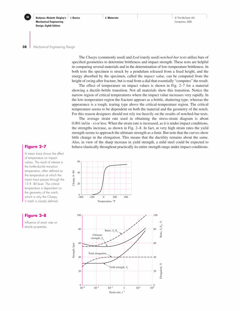
Budynas−Nisbett: Shigley’s
Mechanical Engineering
Design, Eighth Edition
I. Basics 2. Materials44 © The McGraw−Hill
Companies, 2008
38 Mechanical Engineering Design
The Charpy (commonly used) and Izod (rarely used) notched-bar tests utilize bars of
specified geometries to determine brittleness and impact strength. These tests are helpful
in comparing several materials and in the determination of low-temperature brittleness. In
both tests the specimen is struck by a pendulum released from a fixed height, and the
energy absorbed by the specimen, called the impact value, can be computed from the
height of swing after fracture, but is read from a dial that essentially “computes” the result.
The effect of temperature on impact values is shown in Fig. 2–7 for a material
showing a ductile-brittle transition. Not all materials show this transition. Notice the
narrow region of critical temperatures where the impact value increases very rapidly. In
the low-temperature region the fracture appears as a brittle, shattering type, whereas the
appearance is a tough, tearing type above the critical-temperature region. The critical
temperature seems to be dependent on both the material and the geometry of the notch.
For this reason designers should not rely too heavily on the results of notched-bar tests.
The average strain rate used in obtaining the stress-strain diagram is about
0.001 in/(in · s) or less. When the strain rate is increased, as it is under impact conditions,
the strengths increase, as shown in Fig. 2–8. In fact, at very high strain rates the yield
strength seems to approach the ultimate strength as a limit. But note that the curves show
little change in the elongation. This means that the ductility remains about the same.
Also, in view of the sharp increase in yield strength, a mild steel could be expected to
behave elastically throughout practically its entire strength range under impact conditions.
–400 0 200 4000
20
40
60
Char
py,
ft�
lbf
Temperature, °F
–200
Figure 2–7
A mean trace shows the effectof temperature on impactvalues. The result of interest isthe brittle-ductile transitiontemperature, often defined asthe temperature at which themean trace passes through the15 ft · lbf level. The criticaltemperature is dependent onthe geometry of the notch,which is why the CharpyV notch is closely defined.
10–6 10–4 10–2 1 102 1040
20
40
60
80
100
0
20
40
60
80
100
Str
ength
, kpsi
Strain rate, s–1
Rat
io,
Sy/S
u, %
Elo
ngat
ion, %
Ratio, Sy /Su
Ultimate
strength, Su
Total elongation
Yield strength, Sy
Figure 2–8
Influence of strain rate ontensile properties.

Budynas−Nisbett: Shigley’s
Mechanical Engineering
Design, Eighth Edition
I. Basics 2. Materials 45© The McGraw−Hill
Companies, 2008
Materials 39
The Charpy and Izod tests really provide toughness data under dynamic, rather than
static, conditions. It may well be that impact data obtained from these tests are as depen-
dent on the notch geometry as they are on the strain rate. For these reasons it may be bet-
ter to use the concepts of notch sensitivity, fracture toughness, and fracture mechanics,
discussed in Chaps. 5 and 6, to assess the possibility of cracking or fracture.
2–6 Temperature EffectsStrength and ductility, or brittleness, are properties affected by the temperature of the
operating environment.
The effect of temperature on the static properties of steels is typified by the strength
versus temperature chart of Fig. 2–9. Note that the tensile strength changes only a small
amount until a certain temperature is reached. At that point it falls off rapidly. The yield
strength, however, decreases continuously as the environmental temperature is increased.
There is a substantial increase in ductility, as might be expected, at the higher temperatures.
Many tests have been made of ferrous metals subjected to constant loads for long
periods of time at elevated temperatures. The specimens were found to be permanently
deformed during the tests, even though at times the actual stresses were less than the
yield strength of the material obtained from short-time tests made at the same temper-
ature. This continuous deformation under load is called creep.
One of the most useful tests to have been devised is the long-time creep test under
constant load. Figure 2–10 illustrates a curve that is typical of this kind of test. The
curve is obtained at a constant stated temperature. A number of tests are usually run
simultaneously at different stress intensities. The curve exhibits three distinct regions.
In the first stage are included both the elastic and the plastic deformation. This stage shows
a decreasing creep rate, which is due to the strain hardening. The second stage shows
a constant minimum creep rate caused by the annealing effect. In the third stage the
specimen shows a considerable reduction in area, the true stress is increased, and a
higher creep eventually leads to fracture.
When the operating temperatures are lower than the transition temperature
(Fig. 2–7), the possibility arises that a part could fail by a brittle fracture. This subject
will be discussed in Chap. 5.
1.0
0.9
0.8
0.7
0.6
0.50 200 400 600
ST/S
RT
Sy
RTTemperature, °C
Sut
Figure 2–9
A plot of the results of 145 testsof 21 carbon and alloy steelsshowing the effect of operatingtemperature on the yieldstrength Sy and the ultimatestrength Sut . The ordinate is theratio of the strength at theoperating temperature to thestrength at room temperature.The standard deviations were0.0442 ≤ σSy ≤ 0.152 forSy and 0.099 ≤ σSut ≤ 0.11for Sut . (Data source: E. A.Brandes (ed.), Smithells MetalReference Book, 6th ed.,Butterworth, London, 1983pp. 22–128 to 22–131.)

Budynas−Nisbett: Shigley’s
Mechanical Engineering
Design, Eighth Edition
I. Basics 2. Materials46 © The McGraw−Hill
Companies, 2008
40 Mechanical Engineering Design
1st stage2nd stage 3rd stage
Time
Cre
ep d
eform
atio
n
Figure 2–10
Creep-time curve.
Of course, heat treatment, as will be shown, is used to make substantial changes in
the mechanical properties of a material.
Heating due to electric and gas welding also changes the mechanical properties.
Such changes may be due to clamping during the welding process, as well as heating;
the resulting stresses then remain when the parts have cooled and the clamps have been
removed. Hardness tests can be used to learn whether the strength has been changed by
welding, but such tests will not reveal the presence of residual stresses.
2–7 Numbering SystemsThe Society of Automotive Engineers (SAE) was the first to recognize the need, and to
adopt a system, for the numbering of steels. Later the American Iron and Steel Institute
(AISI) adopted a similar system. In 1975 the SAE published the Unified Numbering
System for Metals and Alloys (UNS); this system also contains cross-reference num-
bers for other material specifications.7 The UNS uses a letter prefix to designate the
material, as, for example, G for the carbon and alloy steels, A for the aluminum alloys,
C for the copper-base alloys, and S for the stainless or corrosion-resistant steels. For
some materials, not enough agreement has as yet developed in the industry to warrant
the establishment of a designation.
For the steels, the first two numbers following the letter prefix indicate the compo-
sition, excluding the carbon content. The various compositions used are as follows:
G10 Plain carbon
G11 Free-cutting carbon steel withmore sulfur or phosphorus
G13 Manganese
G23 Nickel
G25 Nickel
G31 Nickel-chromium
G33 Nickel-chromium
G40 Molybdenum
G41 Chromium-molybdenum
G43 Nickel-chromium-molybdenum
G46 Nickel-molybdenum
G48 Nickel-molybdenum
G50 Chromium
G51 Chromium
G52 Chromium
G61 Chromium-vanadium
G86 Chromium-nickel-molybdenum
G87 Chromium-nickel-molybdenum
G92 Manganese-silicon
G94 Nickel-chromium-molybdenum
7Many of the materials discussed in the balance of this chapter are listed in the Appendix tables. Be sure to
review these.

Budynas−Nisbett: Shigley’s
Mechanical Engineering
Design, Eighth Edition
I. Basics 2. Materials 47© The McGraw−Hill
Companies, 2008
Materials 41
The second number pair refers to the approximate carbon content. Thus, G10400 is a
plain carbon steel with a nominal carbon content of 0.40 percent (0.37 to 0.44 percent).
The fifth number following the prefix is used for special situations. For example, the old
designation AISI 52100 represents a chromium alloy with about 100 points of carbon.
The UNS designation is G52986.
The UNS designations for the stainless steels, prefix S, utilize the older AISI des-
ignations for the first three numbers following the prefix. The next two numbers are
reserved for special purposes. The first number of the group indicates the approximate
composition. Thus 2 is a chromium-nickel-manganese steel, 3 is a chromium-nickel
steel, and 4 is a chromium alloy steel. Sometimes stainless steels are referred to by their
alloy content. Thus S30200 is often called an 18-8 stainless steel, meaning 18 percent
chromium and 8 percent nickel.
The prefix for the aluminum group is the letter A. The first number following the
prefix indicates the processing. For example, A9 is a wrought aluminum, while A0 is
a casting alloy. The second number designates the main alloy group as shown in
Table 2–1. The third number in the group is used to modify the original alloy or to
designate the impurity limits. The last two numbers refer to other alloys used with the
basic group.
The American Society for Testing and Materials (ASTM) numbering system for
cast iron is in widespread use. This system is based on the tensile strength. Thus ASTM
A18 speaks of classes; e.g., 30 cast iron has a minimum tensile strength of 30 kpsi. Note
from Appendix A-24, however, that the typical tensile strength is 31 kpsi. You should
be careful to designate which of the two values is used in design and problem work
because of the significance of factor of safety.
2–8 Sand CastingSand casting is a basic low-cost process, and it lends itself to economical production
in large quantities with practically no limit to the size, shape, or complexity of the part
produced.
In sand casting, the casting is made by pouring molten metal into sand molds. A
pattern, constructed of metal or wood, is used to form the cavity into which the molten
metal is poured. Recesses or holes in the casting are produced by sand cores introduced
into the mold. The designer should make an effort to visualize the pattern and casting
in the mold. In this way the problems of core setting, pattern removal, draft, and solid-
ification can be studied. Castings to be used as test bars of cast iron are cast separately
and properties may vary.
Table 2–1
Aluminum Alloy
Designations
Aluminum 99.00% pure and greater Ax1xxx
Copper alloys Ax2xxx
Manganese alloys Ax3xxx
Silicon alloys Ax4xxx
Magnesium alloys Ax5xxx
Magnesium-silicon alloys Ax6xxx
Zinc alloys Ax7xxx

Budynas−Nisbett: Shigley’s
Mechanical Engineering
Design, Eighth Edition
I. Basics 2. Materials48 © The McGraw−Hill
Companies, 2008
42 Mechanical Engineering Design
Steel castings are the most difficult of all to produce, because steel has the highest
melting temperature of all materials normally used for casting. This high temperature
aggravates all casting problems.
The following rules will be found quite useful in the design of any sand casting:
1 All sections should be designed with a uniform thickness.
2 The casting should be designed so as to produce a gradual change from section
to section where this is necessary.
3 Adjoining sections should be designed with generous fillets or radii.
4 A complicated part should be designed as two or more simple castings to be
assembled by fasteners or by welding.
Steel, gray iron, brass, bronze, and aluminum are most often used in castings. The
minimum wall thickness for any of these materials is about 5 mm, though with partic-
ular care, thinner sections can be obtained with some materials.
2–9 Shell MoldingThe shell-molding process employs a heated metal pattern, usually made of cast iron,
aluminum, or brass, which is placed in a shell-molding machine containing a mixture
of dry sand and thermosetting resin. The hot pattern melts the plastic, which, together
with the sand, forms a shell about 5 to 10 mm thick around the pattern. The shell is then
baked at from 400 to 700°F for a short time while still on the pattern. It is then stripped
from the pattern and placed in storage for use in casting.
In the next step the shells are assembled by clamping, bolting, or pasting; they are
placed in a backup material, such as steel shot; and the molten metal is poured into the
cavity. The thin shell permits the heat to be conducted away so that solidification takes
place rapidly. As solidification takes place, the plastic bond is burned and the mold col-
lapses. The permeability of the backup material allows the gases to escape and the cast-
ing to air-cool. All this aids in obtaining a fine-grain, stress-free casting.
Shell-mold castings feature a smooth surface, a draft that is quite small, and close
tolerances. In general, the rules governing sand casting also apply to shell-mold casting.
2–10 Investment CastingInvestment casting uses a pattern that may be made from wax, plastic, or other material.
After the mold is made, the pattern is melted out. Thus a mechanized method of casting
a great many patterns is necessary. The mold material is dependent upon the melting
point of the cast metal. Thus a plaster mold can be used for some materials while
others would require a ceramic mold. After the pattern is melted out, the mold is baked
or fired; when firing is completed, the molten metal may be poured into the hot mold
and allowed to cool.
If a number of castings are to be made, then metal or permanent molds may be suit-
able. Such molds have the advantage that the surfaces are smooth, bright, and accurate,
so that little, if any, machining is required. Metal-mold castings are also known as die
castings and centrifugal castings.
2–11 Powder-Metallurgy ProcessThe powder-metallurgy process is a quantity-production process that uses powders
from a single metal, several metals, or a mixture of metals and nonmetals. It consists
essentially of mechanically mixing the powders, compacting them in dies at high pressures,

Budynas−Nisbett: Shigley’s
Mechanical Engineering
Design, Eighth Edition
I. Basics 2. Materials 49© The McGraw−Hill
Companies, 2008
Materials 43
and heating the compacted part at a temperature less than the melting point of the major
ingredient. The particles are united into a single strong part similar to what would be
obtained by melting the same ingredients together. The advantages are (1) the elimina-
tion of scrap or waste material, (2) the elimination of machining operations, (3) the low
unit cost when mass-produced, and (4) the exact control of composition. Some of the
disadvantages are (1) the high cost of dies, (2) the lower physical properties, (3) the
higher cost of materials, (4) the limitations on the design, and (5) the limited range of
materials that can be used. Parts commonly made by this process are oil-impregnated
bearings, incandescent lamp filaments, cemented-carbide tips for tools, and permanent
magnets. Some products can be made only by powder metallurgy: surgical implants, for
example. The structure is different from what can be obtained by melting the same
ingredients.
2–12 Hot-Working ProcessesBy hot working are meant such processes as rolling, forging, hot extrusion, and hot
pressing, in which the metal is heated above its recrystallation temperature.
Hot rolling is usually used to create a bar of material of a particular shape and
dimension. Figure 2–11 shows some of the various shapes that are commonly produced
by the hot-rolling process. All of them are available in many different sizes as well as
in different materials. The materials most available in the hot-rolled bar sizes are steel,
aluminum, magnesium, and copper alloys.
Tubing can be manufactured by hot-rolling strip or plate. The edges of the strip are
rolled together, creating seams that are either butt-welded or lap-welded. Seamless tub-
ing is manufactured by roll-piercing a solid heated rod with a piercing mandrel.
Extrusion is the process by which great pressure is applied to a heated metal billet
or blank, causing it to flow through a restricted orifice. This process is more common
with materials of low melting point, such as aluminum, copper, magnesium, lead, tin,
and zinc. Stainless steel extrusions are available on a more limited basis.
Forging is the hot working of metal by hammers, presses, or forging machines. In
common with other hot-working processes, forging produces a refined grain structure
that results in increased strength and ductility. Compared with castings, forgings have
greater strength for the same weight. In addition, drop forgings can be made smoother
and more accurate than sand castings, so that less machining is necessary. However, the
initial cost of the forging dies is usually greater than the cost of patterns for castings,
although the greater unit strength rather than the cost is usually the deciding factor
between these two processes.
Round Square Half oval
(a) Bar shapes
Flat Hexagon
(b) Structural shapes
Wide flange Channel Angle Tee Zee
Figure 2–11
Common shapes availablethrough hot rolling.

Budynas−Nisbett: Shigley’s
Mechanical Engineering
Design, Eighth Edition
I. Basics 2. Materials50 © The McGraw−Hill
Companies, 2008
44 Mechanical Engineering Design
2–13 Cold-Working ProcessesBy cold working is meant the forming of the metal while at a low temperature (usually
room temperature). In contrast to parts produced by hot working, cold-worked parts
have a bright new finish, are more accurate, and require less machining.
Cold-finished bars and shafts are produced by rolling, drawing, turning, grinding,
and polishing. Of these methods, by far the largest percentage of products are made by
the cold-rolling and cold-drawing processes. Cold rolling is now used mostly for the
production of wide flats and sheets. Practically all cold-finished bars are made by cold
drawing but even so are sometimes mistakenly called “cold-rolled bars.” In the drawing
process, the hot-rolled bars are first cleaned of scale and then drawn by pulling them
through a die that reduces the size about 132
to 116
in. This process does not remove
material from the bar but reduces, or “draws” down, the size. Many different shapes of
hot-rolled bars may be used for cold drawing.
Cold rolling and cold drawing have the same effect upon the mechanical proper-
ties. The cold-working process does not change the grain size but merely distorts it.
Cold working results in a large increase in yield strength, an increase in ultimate
strength and hardness, and a decrease in ductility. In Fig. 2–12 the properties of a cold-
drawn bar are compared with those of a hot-rolled bar of the same material.
Heading is a cold-working process in which the metal is gathered, or upset. This
operation is commonly used to make screw and rivet heads and is capable of producing
a wide variety of shapes. Roll threading is the process of rolling threads by squeezing
and rolling a blank between two serrated dies. Spinning is the operation of working sheet
material around a rotating form into a circular shape. Stamping is the term used to
describe punch-press operations such as blanking, coining, forming, and shallow
drawing.
2–14 The Heat Treatment of SteelHeat treatment of steel refers to time- and temperature-controlled processes that relieve
residual stresses and/or modifies material properties such as hardness (strength), duc-
tility, and toughness. Other mechanical or chemical operations are sometimes grouped
under the heading of heat treatment. The common heat-treating operations are anneal-
ing, quenching, tempering, and case hardening.
0 0.2 0.4 0.60
20
40
60
80
100
Elongation, in
Str
ength
, kpsi
Yield point
Yield point
Cold-drawn
Hot-rolled
Figure 2–12
Stress-strain diagram forhot-rolled and cold-drawnUNS G10350 steel.

Budynas−Nisbett: Shigley’s
Mechanical Engineering
Design, Eighth Edition
I. Basics 2. Materials 51© The McGraw−Hill
Companies, 2008
Materials 45
Annealing
When a material is cold- or hot-worked, residual stresses are built in, and, in addition,
the material usually has a higher hardness as a result of these working operations. These
operations change the structure of the material so that it is no longer represented by the
equilibrium diagram. Full annealing and normalizing is a heating operation that permits
the material to transform according to the equilibrium diagram. The material to be
annealed is heated to a temperature that is approximately 100°F above the critical tem-
perature. It is held at this temperature for a time that is sufficient for the carbon to
become dissolved and diffused through the material. The object being treated is then
allowed to cool slowly, usually in the furnace in which it was treated. If the transfor-
mation is complete, then it is said to have a full anneal. Annealing is used to soften a
material and make it more ductile, to relieve residual stresses, and to refine the grain
structure.
The term annealing includes the process called normalizing. Parts to be normalized
may be heated to a slightly higher temperature than in full annealing. This produces a
coarser grain structure, which is more easily machined if the material is a low-carbon
steel. In the normalizing process the part is cooled in still air at room temperature. Since
this cooling is more rapid than the slow cooling used in full annealing, less time is avail-
able for equilibrium, and the material is harder than fully annealed steel. Normalizing
is often used as the final treating operation for steel. The cooling in still air amounts to
a slow quench.
Quenching
Eutectoid steel that is fully annealed consists entirely of pearlite, which is obtained
from austenite under conditions of equilibrium. A fully annealed hypoeutectoid steel
would consist of pearlite plus ferrite, while hypereutectoid steel in the fully annealed
condition would consist of pearlite plus cementite. The hardness of steel of a given
carbon content depends upon the structure that replaces the pearlite when full anneal-
ing is not carried out.
The absence of full annealing indicates a more rapid rate of cooling. The rate of
cooling is the factor that determines the hardness. A controlled cooling rate is called
quenching. A mild quench is obtained by cooling in still air, which, as we have seen, is
obtained by the normalizing process. The two most widely used media for quenching
are water and oil. The oil quench is quite slow but prevents quenching cracks caused by
rapid expansion of the object being treated. Quenching in water is used for carbon steels
and for medium-carbon, low-alloy steels.
The effectiveness of quenching depends upon the fact that when austenite is cooled
it does not transform into pearlite instantaneously but requires time to initiate and com-
plete the process. Since the transformation ceases at about 800°F, it can be prevented
by rapidly cooling the material to a lower temperature. When the material is cooled
rapidly to 400°F or less, the austenite is transformed into a structure called martensite.
Martensite is a supersaturated solid solution of carbon in ferrite and is the hardest and
strongest form of steel.
If steel is rapidly cooled to a temperature between 400 and 800°F and held there
for a sufficient length of time, the austenite is transformed into a material that is gener-
ally called bainite. Bainite is a structure intermediate between pearlite and martensite.
Although there are several structures that can be identified between the temperatures
given, depending upon the temperature used, they are collectively known as bainite. By
the choice of this transformation temperature, almost any variation of structure may be
obtained. These range all the way from coarse pearlite to fine martensite.

Budynas−Nisbett: Shigley’s
Mechanical Engineering
Design, Eighth Edition
I. Basics 2. Materials52 © The McGraw−Hill
Companies, 2008
46 Mechanical Engineering Design
Tempering
When a steel specimen has been fully hardened, it is very hard and brittle and has high
residual stresses. The steel is unstable and tends to contract on aging. This tendency
is increased when the specimen is subjected to externally applied loads, because the
resultant stresses contribute still more to the instability. These internal stresses can
be relieved by a modest heating process called stress relieving, or a combination of
stress relieving and softening called tempering or drawing. After the specimen has been
fully hardened by being quenched from above the critical temperature, it is reheated to
some temperature below the critical temperature for a certain period of time and then
allowed to cool in still air. The temperature to which it is reheated depends upon the
composition and the degree of hardness or toughness desired.8 This reheating operation
releases the carbon held in the martensite, forming carbide crystals. The structure
obtained is called tempered martensite. It is now essentially a superfine dispersion of
iron carbide(s) in fine-grained ferrite.
The effect of heat-treating operations upon the various mechanical properties of a
low alloy steel is shown graphically in Fig. 2–13.
50
100
150
200
250
300
300
400
500
600
200 400 600 800 1000 1200 14000
20
40
60
80
Tempering temperature, °F
Bri
nel
l har
dnes
s
Per
cent
elongat
ion a
nd
reduct
ion i
n a
rea
Ten
sile
and y
ield
str
ength
, kpsi
Condition
Normalized
As rolled
Annealed
Tensile
strength,
kpsi
Yield
strength,
kpsi
Reduction
in area,
%
Elongation
in 2 in,
%
Brinell
hardness,
Bhn
200
190
120
147
144
99
20
18
43
10
9
18
410
380
228
Tensile strength
Yield strength
Brinell
Reduction area
Elongation
Figure 2–13
The effect of thermal-mechanical history on themechanical properties of AISI4340 steel. (Prepared by theInternational Nickel Company.)
8For the quantitative aspects of tempering in plain carbon and low-alloy steels, see Charles R. Mischke,
“The Strength of Cold-Worked and Heat-Treated Steels,” Chap. 33 in Joseph E. Shigley, Charles R.
Mischke, and Thomas H. Brown, Jr. (eds.), Standard Handbook of Machine Design, 3rd ed., McGraw-Hill,
New York, 2004.

Budynas−Nisbett: Shigley’s
Mechanical Engineering
Design, Eighth Edition
I. Basics 2. Materials 53© The McGraw−Hill
Companies, 2008
Materials 47
9W. Crafts and J. L. Lamont, Hardenability and Steel Selection, Pitman and Sons, London, 1949.
10Charles R. Mischke, Chap. 33 in Joseph E. Shigley, Charles R. Mischke, and Thomas H. Brown, Jr. (eds.),
Standard Handbook of Machine Design, 3rd ed., McGraw-Hill, New York, 2004, p. 33.9.11M. A. Grossman, AIME, February 1942.
12J. Field, Metals Progress, March 1943.
13Modern Steels and Their Properties, 7th ed., Handbook 2757, Bethlehem Steel, 1972, pp. 46–50.
Case Hardening
The purpose of case hardening is to produce a hard outer surface on a specimen of low-
carbon steel while at the same time retaining the ductility and toughness in the core.
This is done by increasing the carbon content at the surface. Either solid, liquid, or
gaseous carburizing materials may be used. The process consists of introducing the part
to be carburized into the carburizing material for a stated time and at a stated tempera-
ture, depending upon the depth of case desired and the composition of the part. The part
may then be quenched directly from the carburization temperature and tempered, or in
some cases it must undergo a double heat treatment in order to ensure that both the core
and the case are in proper condition. Some of the more useful case-hardening processes
are pack carburizing, gas carburizing, nitriding, cyaniding, induction hardening, and
flame hardening. In the last two cases carbon is not added to the steel in question, gen-
erally a medium carbon steel, for example SAE/AISI 1144.
Quantitative Estimation of Properties of Heat-Treated Steels
Courses in metallurgy (or material science) for mechanical engineers usually present the
addition method of Crafts and Lamont for the prediction of heat-treated properties from the
Jominy test for plain carbon steels.9 If this has not been in your prerequisite experience,
then refer to the Standard Handbook of Machine Design, where the addition method is cov-
ered with examples.10 If this book is a textbook for a machine elements course, it is a good
class project (many hands make light work) to study the method and report to the class.
For low-alloy steels, the multiplication method of Grossman11 and Field12 is
explained in the Standard Handbook of Machine Design (Secs. 29.6 and 33.6).
Modern Steels and Their Properties Handbook explains how to predict the Jominy
curve by the method of Grossman and Field from a ladle analysis and grain size.13
Bethlehem Steel has developed a circular plastic slide rule that is convenient to the purpose.
2–15 Alloy SteelsAlthough a plain carbon steel is an alloy of iron and carbon with small amounts of
manganese, silicon, sulfur, and phosphorus, the term alloy steel is applied when one or
more elements other than carbon are introduced in sufficient quantities to modify its
properties substantially. The alloy steels not only possess more desirable physical
properties but also permit a greater latitude in the heat-treating process.
Chromium
The addition of chromium results in the formation of various carbides of chromium that
are very hard, yet the resulting steel is more ductile than a steel of the same hardness pro-
duced by a simple increase in carbon content. Chromium also refines the grain structure
so that these two combined effects result in both increased toughness and increased hard-
ness. The addition of chromium increases the critical range of temperatures and moves
the eutectoid point to the left. Chromium is thus a very useful alloying element.

Budynas−Nisbett: Shigley’s
Mechanical Engineering
Design, Eighth Edition
I. Basics 2. Materials54 © The McGraw−Hill
Companies, 2008
48 Mechanical Engineering Design
Nickel
The addition of nickel to steel also causes the eutectoid point to move to the left and
increases the critical range of temperatures. Nickel is soluble in ferrite and does not
form carbides or oxides. This increases the strength without decreasing the ductility.
Case hardening of nickel steels results in a better core than can be obtained with plain
carbon steels. Chromium is frequently used in combination with nickel to obtain the
toughness and ductility provided by the nickel and the wear resistance and hardness
contributed by the chromium.
Manganese
Manganese is added to all steels as a deoxidizing and desulfurizing agent, but if the sul-
fur content is low and the manganese content is over 1 percent, the steel is classified as a
manganese alloy. Manganese dissolves in the ferrite and also forms carbides. It causes
the eutectoid point to move to the left and lowers the critical range of temperatures. It
increases the time required for transformation so that oil quenching becomes practicable.
Silicon
Silicon is added to all steels as a deoxidizing agent. When added to very-low-carbon
steels, it produces a brittle material with a low hysteresis loss and a high magnetic
permeability. The principal use of silicon is with other alloying elements, such as
manganese, chromium, and vanadium, to stabilize the carbides.
Molybdenum
While molybdenum is used alone in a few steels, it finds its greatest use when combined
with other alloying elements, such as nickel, chromium, or both. Molybdenum forms
carbides and also dissolves in ferrite to some extent, so that it adds both hardness and
toughness. Molybdenum increases the critical range of temperatures and substantially
lowers the transformation point. Because of this lowering of the transformation point,
molybdenum is most effective in producing desirable oil-hardening and air-hardening
properties. Except for carbon, it has the greatest hardening effect, and because it also
contributes to a fine grain size, this results in the retention of a great deal of toughness.
Vanadium
Vanadium has a very strong tendency to form carbides; hence it is used only in small
amounts. It is a strong deoxidizing agent and promotes a fine grain size. Since some vana-
dium is dissolved in the ferrite, it also toughens the steel. Vanadium gives a wide harden-
ing range to steel, and the alloy can be hardened from a higher temperature. It is very
difficult to soften vanadium steel by tempering; hence, it is widely used in tool steels.
Tungsten
Tungsten is widely used in tool steels because the tool will maintain its hardness even
at red heat. Tungsten produces a fine, dense structure and adds both toughness and hard-
ness. Its effect is similar to that of molybdenum, except that it must be added in greater
quantities.
2–16 Corrosion-Resistant SteelsIron-base alloys containing at least 12 percent chromium are called stainless steels.
The most important characteristic of these steels is their resistance to many, but not all,
corrosive conditions. The four types available are the ferritic chromium steels, the

Budynas−Nisbett: Shigley’s
Mechanical Engineering
Design, Eighth Edition
I. Basics 2. Materials 55© The McGraw−Hill
Companies, 2008
Materials 49
austenitic chromium-nickel steels, and the martensitic and precipitation-hardenable
stainless steels.
The ferritic chromium steels have a chromium content ranging from 12 to 27 per-
cent. Their corrosion resistance is a function of the chromium content, so that alloys
containing less than 12 percent still exhibit some corrosion resistance, although they
may rust. The quench-hardenability of these steels is a function of both the chromium
and the carbon content. The very high carbon steels have good quench hardenability up
to about 18 percent chromium, while in the lower carbon ranges it ceases at about
13 percent. If a little nickel is added, these steels retain some degree of hardenability up
to 20 percent chromium. If the chromium content exceeds 18 percent, they become dif-
ficult to weld, and at the very high chromium levels the hardness becomes so great that
very careful attention must be paid to the service conditions. Since chromium is expen-
sive, the designer will choose the lowest chromium content consistent with the corro-
sive conditions.
The chromium-nickel stainless steels retain the austenitic structure at room tem-
perature; hence, they are not amenable to heat treatment. The strength of these steels
can be greatly improved by cold working. They are not magnetic unless cold-worked.
Their work hardenability properties also cause them to be difficult to machine. All
the chromium-nickel steels may be welded. They have greater corrosion-resistant prop-
erties than the plain chromium steels. When more chromium is added for greater cor-
rosion resistance, more nickel must also be added if the austenitic properties are to be
retained.
2–17 Casting MaterialsGray Cast Iron
Of all the cast materials, gray cast iron is the most widely used. This is because it has
a very low cost, is easily cast in large quantities, and is easy to machine. The principal
objections to the use of gray cast iron are that it is brittle and that it is weak in tension.
In addition to a high carbon content (over 1.7 percent and usually greater than 2 percent),
cast iron also has a high silicon content, with low percentages of sulfur, manganese,
and phosphorus. The resultant alloy is composed of pearlite, ferrite, and graphite, and
under certain conditions the pearlite may decompose into graphite and ferrite. The
resulting product then contains all ferrite and graphite. The graphite, in the form of
thin flakes distributed evenly throughout the structure, darkens it; hence, the name gray
cast iron.
Gray cast iron is not readily welded, because it may crack, but this tendency may
be reduced if the part is carefully preheated. Although the castings are generally used in
the as-cast condition, a mild anneal reduces cooling stresses and improves the machin-
ability. The tensile strength of gray cast iron varies from 100 to 400 MPa (15 to 60 kpsi),
and the compressive strengths are 3 to 4 times the tensile strengths. The modulus of
elasticity varies widely, with values extending all the way from 75 to 150 GPa (11 to
22 Mpsi).
Ductile and Nodular Cast Iron
Because of the lengthy heat treatment required to produce malleable cast iron, engineers
have long desired a cast iron that would combine the ductile properties of malleable
iron with the ease of casting and machining of gray iron and at the same time would
possess these properties in the as-cast conditions. A process for producing such a material
using magnesium-containing material seems to fulfill these requirements.

Budynas−Nisbett: Shigley’s
Mechanical Engineering
Design, Eighth Edition
I. Basics 2. Materials56 © The McGraw−Hill
Companies, 2008
50 Mechanical Engineering Design
Ductile cast iron, or nodular cast iron, as it is sometimes called, is essentially the
same as malleable cast iron, because both contain graphite in the form of spheroids.
However, ductile cast iron in the as-cast condition exhibits properties very close to
those of malleable iron, and if a simple 1-h anneal is given and is followed by a slow
cool, it exhibits even more ductility than the malleable product. Ductile iron is made by
adding MgFeSi to the melt; since magnesium boils at this temperature, it is necessary
to alloy it with other elements before it is introduced.
Ductile iron has a high modulus of elasticity (172 GPa or 25 Mpsi) as compared
with gray cast iron, and it is elastic in the sense that a portion of the stress-strain
curve is a straight line. Gray cast iron, on the other hand, does not obey Hooke’s law,
because the modulus of elasticity steadily decreases with increase in stress. Like
gray cast iron, however, nodular iron has a compressive strength that is higher than
the tensile strength, although the difference is not as great. In 40 years it has become
extensively used.
White Cast Iron
If all the carbon in cast iron is in the form of cementite and pearlite, with no graphite
present, the resulting structure is white and is known as white cast iron. This may be
produced in two ways. The composition may be adjusted by keeping the carbon and
silicon content low, or the gray-cast-iron composition may be cast against chills in order
to promote rapid cooling. By either method, a casting with large amounts of cementite
is produced, and as a result the product is very brittle and hard to machine but also very
resistant to wear. A chill is usually used in the production of gray-iron castings in order
to provide a very hard surface within a particular area of the casting, while at the same
time retaining the more desirable gray structure within the remaining portion. This pro-
duces a relatively tough casting with a wear-resistant area.
Malleable Cast Iron
If white cast iron within a certain composition range is annealed, a product called
malleable cast iron is formed. The annealing process frees the carbon so that it is pre-
sent as graphite, just as in gray cast iron but in a different form. In gray cast iron the
graphite is present in a thin flake form, while in malleable cast iron it has a nodular
form and is known as temper carbon. A good grade of malleable cast iron may have
a tensile strength of over 350 MPa (50 kpsi), with an elongation of as much as 18 per-
cent. The percentage elongation of a gray cast iron, on the other hand, is seldom over
1 percent. Because of the time required for annealing (up to 6 days for large and
heavy castings), malleable iron is necessarily somewhat more expensive than gray
cast iron.
Alloy Cast Irons
Nickel, chromium, and molybdenum are the most common alloying elements used in
cast iron. Nickel is a general-purpose alloying element, usually added in amounts up to
5 percent. Nickel increases the strength and density, improves the wearing qualities, and
raises the machinability. If the nickel content is raised to 10 to 18 percent, an austenitic
structure with valuable heat- and corrosion-resistant properties results. Chromium
increases the hardness and wear resistance and, when used with a chill, increases the
tendency to form white iron. When chromium and nickel are both added, the hardness
and strength are improved without a reduction in the machinability rating. Molybdenum
added in quantities up to 1.25 percent increases the stiffness, hardness, tensile strength,
and impact resistance. It is a widely used alloying element.
Budynas−Nisbett: Shigley’s
Mechanical Engineering
Design, Eighth Edition
I. Basics 2. Materials 57© The McGraw−Hill
Companies, 2008
Materials 51
Cast Steels
The advantage of the casting process is that parts having complex shapes can be man-
ufactured at costs less than fabrication by other means, such as welding. Thus the
choice of steel castings is logical when the part is complex and when it must also have
a high strength. The higher melting temperatures for steels do aggravate the casting
problems and require closer attention to such details as core design, section thicknesses,
fillets, and the progress of cooling. The same alloying elements used for the wrought
steels can be used for cast steels to improve the strength and other mechanical proper-
ties. Cast-steel parts can also be heat-treated to alter the mechanical properties, and,
unlike the cast irons, they can be welded.
2–18 Nonferrous MetalsAluminum
The outstanding characteristics of aluminum and its alloys are their strength-weight
ratio, their resistance to corrosion, and their high thermal and electrical conductivity.
The density of aluminum is about 2770 kg/m3 (0.10 lbf/in3), compared with 7750 kg/m3
(0.28 lbf/in3) for steel. Pure aluminum has a tensile strength of about 90 MPa (13 kpsi),
but this can be improved considerably by cold working and also by alloying with other
materials. The modulus of elasticity of aluminum, as well as of its alloys, is 71.7 GPa
(10.4 Mpsi), which means that it has about one-third the stiffness of steel.
Considering the cost and strength of aluminum and its alloys, they are among the
most versatile materials from the standpoint of fabrication. Aluminum can be processed
by sand casting, die casting, hot or cold working, or extruding. Its alloys can be machined,
press-worked, soldered, brazed, or welded. Pure aluminum melts at 660°C (1215°F),
which makes it very desirable for the production of either permanent or sand-mold
castings. It is commercially available in the form of plate, bar, sheet, foil, rod, and tube
and in structural and extruded shapes. Certain precautions must be taken in joining
aluminum by soldering, brazing, or welding; these joining methods are not recommended
for all alloys.
The corrosion resistance of the aluminum alloys depends upon the formation of a
thin oxide coating. This film forms spontaneously because aluminum is inherently very
reactive. Constant erosion or abrasion removes this film and allows corrosion to take
place. An extra-heavy oxide film may be produced by the process called anodizing. In
this process the specimen is made to become the anode in an electrolyte, which may be
chromic acid, oxalic acid, or sulfuric acid. It is possible in this process to control the
color of the resulting film very accurately.
The most useful alloying elements for aluminum are copper, silicon, manganese,
magnesium, and zinc. Aluminum alloys are classified as casting alloys or wrought
alloys. The casting alloys have greater percentages of alloying elements to facilitate
casting, but this makes cold working difficult. Many of the casting alloys, and some of
the wrought alloys, cannot be hardened by heat treatment. The alloys that are heat-
treatable use an alloying element that dissolves in the aluminum. The heat treatment
consists of heating the specimen to a temperature that permits the alloying element to
pass into solution, then quenching so rapidly that the alloying element is not precipi-
tated. The aging process may be accelerated by heating slightly, which results in even
greater hardness and strength. One of the better-known heat-treatable alloys is duralu-
minum, or 2017 (4 percent Cu, 0.5 percent Mg, 0.5 percent Mn). This alloy hardens in
4 days at room temperature. Because of this rapid aging, the alloy must be stored under

Budynas−Nisbett: Shigley’s
Mechanical Engineering
Design, Eighth Edition
I. Basics 2. Materials58 © The McGraw−Hill
Companies, 2008
52 Mechanical Engineering Design
refrigeration after quenching and before forming, or it must be formed immediately
after quenching. Other alloys (such as 5053) have been developed that age-harden much
more slowly, so that only mild refrigeration is required before forming. After forming,
they are artificially aged in a furnace and possess approximately the same strength and
hardness as the 2024 alloys. Those alloys of aluminum that cannot be heat-treated can
be hardened only by cold working. Both work hardening and the hardening produced
by heat treatment may be removed by an annealing process.
Magnesium
The density of magnesium is about 1800 kg/m3 (0.065 lb/in3), which is two-thirds that
of aluminum and one-fourth that of steel. Since it is the lightest of all commercial met-
als, its greatest use is in the aircraft and automotive industries, but other uses are now
being found for it. Although the magnesium alloys do not have great strength, because
of their light weight the strength-weight ratio compares favorably with the stronger
aluminum and steel alloys. Even so, magnesium alloys find their greatest use in appli-
cations where strength is not an important consideration. Magnesium will not withstand
elevated temperatures; the yield point is definitely reduced when the temperature is
raised to that of boiling water.
Magnesium and its alloys have a modulus of elasticity of 45 GPa (6.5 Mpsi) in ten-
sion and in compression, although some alloys are not as strong in compression as in
tension. Curiously enough, cold working reduces the modulus of elasticity. A range of
cast magnesium alloys are also available.
Titanium
Titanium and its alloys are similar in strength to moderate-strength steel but weigh half
as much as steel. The material exhibits very good resistence to corrosion, has low ther-
mal conductivity, is nonmagnetic, and has high-temperature strength. Its modulus of
elasticity is between those of steel and aluminum at 16.5 Mpsi (114 GPa). Because of
its many advantages over steel and aluminum, applications include: aerospace and mil-
itary aircraft structures and components, marine hardware, chemical tanks and process-
ing equipment, fluid handling systems, and human internal replacement devices. The
disadvantages of titanium are its high cost compared to steel and aluminum and the dif-
ficulty of machining it.
Copper-Base Alloys
When copper is alloyed with zinc, it is usually called brass. If it is alloyed with another
element, it is often called bronze. Sometimes the other element is specified too, as, for ex-
ample, tin bronze or phosphor bronze. There are hundreds of variations in each category.
Brass with 5 to 15 Percent Zinc
The low-zinc brasses are easy to cold work, especially those with the higher zinc con-
tent. They are ductile but often hard to machine. The corrosion resistance is good. Alloys
included in this group are gilding brass (5 percent Zn), commercial bronze (10 percent Zn),
and red brass (15 percent Zn). Gilding brass is used mostly for jewelry and articles to
be gold-plated; it has the same ductility as copper but greater strength, accompanied by
poor machining characteristics. Commercial bronze is used for jewelry and for forgings
and stampings, because of its ductility. Its machining properties are poor, but it has
excellent cold-working properties. Red brass has good corrosion resistance as well as
high-temperature strength. Because of this it is used a great deal in the form of tubing or
piping to carry hot water in such applications as radiators or condensers.

Budynas−Nisbett: Shigley’s
Mechanical Engineering
Design, Eighth Edition
I. Basics 2. Materials 59© The McGraw−Hill
Companies, 2008
Materials 53
Brass with 20 to 36 Percent Zinc
Included in the intermediate-zinc group are low brass (20 percent Zn), cartridge brass
(30 percent Zn), and yellow brass (35 percent Zn). Since zinc is cheaper than copper,
these alloys cost less than those with more copper and less zinc. They also have better
machinability and slightly greater strength; this is offset, however, by poor corrosion
resistance and the possibility of cracking at points of residual stresses. Low brass is very
similar to red brass and is used for articles requiring deep-drawing operations. Of the
copper-zinc alloys, cartridge brass has the best combination of ductility and strength.
Cartridge cases were originally manufactured entirely by cold working; the process
consisted of a series of deep draws, each draw being followed by an anneal to place the
material in condition for the next draw, hence the name cartridge brass. Although the
hot-working ability of yellow brass is poor, it can be used in practically any other fab-
ricating process and is therefore employed in a large variety of products.
When small amounts of lead are added to the brasses, their machinability is greatly
improved and there is some improvement in their abilities to be hot-worked. The
addition of lead impairs both the cold-working and welding properties. In this group are
low-leaded brass (32 12
percent Zn, 12
percent Pb), high-leaded brass (34 percent Zn,
2 percent Pb), and free-cutting brass (35 12
percent Zn, 3 percent Pb). The low-leaded
brass is not only easy to machine but has good cold-working properties. It is used for
various screw-machine parts. High-leaded brass, sometimes called engraver’s brass, is
used for instrument, lock, and watch parts. Free-cutting brass is also used for screw-
machine parts and has good corrosion resistance with excellent mechanical properties.
Admiralty metal (28 percent Zn) contains 1 percent tin, which imparts excellent
corrosion resistance, especially to saltwater. It has good strength and ductility but only
fair machining and working characteristics. Because of its corrosion resistance it is used
in power-plant and chemical equipment. Aluminum brass (22 percent Zn) contains
2 percent aluminum and is used for the same purposes as admiralty metal, because it
has nearly the same properties and characteristics. In the form of tubing or piping, it is
favored over admiralty metal, because it has better resistance to erosion caused by high-
velocity water.
Brass with 36 to 40 Percent Zinc
Brasses with more than 38 percent zinc are less ductile than cartridge brass and cannot
be cold-worked as severely. They are frequently hot-worked and extruded. Muntz metal
(40 percent Zn) is low in cost and mildly corrosion-resistant. Naval brass has the same
composition as Muntz metal except for the addition of 0.75 percent tin, which con-
tributes to the corrosion resistance.
Bronze
Silicon bronze, containing 3 percent silicon and 1 percent manganese in addition to the
copper, has mechanical properties equal to those of mild steel, as well as good corro-
sion resistance. It can be hot- or cold-worked, machined, or welded. It is useful wher-
ever corrosion resistance combined with strength is required.
Phosphor bronze, made with up to 11 percent tin and containing small amounts of
phosphorus, is especially resistant to fatigue and corrosion. It has a high tensile strength
and a high capacity to absorb energy, and it is also resistant to wear. These properties
make it very useful as a spring material.
Aluminum bronze is a heat-treatable alloy containing up to 12 percent aluminum. This
alloy has strength and corrosion-resistance properties that are better than those of brass, and
in addition, its properties may be varied over a wide range by cold working, heat treating,

Budynas−Nisbett: Shigley’s
Mechanical Engineering
Design, Eighth Edition
I. Basics 2. Materials60 © The McGraw−Hill
Companies, 2008
54 Mechanical Engineering Design
or changing the composition. When iron is added in amounts up to 4 percent, the alloy has
a high endurance limit, a high shock resistance, and excellent wear resistance.
Beryllium bronze is another heat-treatable alloy, containing about 2 percent beryl-
lium. This alloy is very corrosion resistant and has high strength, hardness, and resis-
tance to wear. Although it is expensive, it is used for springs and other parts subjected
to fatigue loading where corrosion resistance is required.
With slight modification most copper-based alloys are available in cast form.
2–19 PlasticsThe term thermoplastics is used to mean any plastic that flows or is moldable when heat
is applied to it; the term is sometimes applied to plastics moldable under pressure. Such
plastics can be remolded when heated.
A thermoset is a plastic for which the polymerization process is finished in a hot
molding press where the plastic is liquefied under pressure. Thermoset plastics cannot
be remolded.
Table 2–2 lists some of the most widely used thermoplastics, together with some
of their characteristics and the range of their properties. Table 2–3, listing some of the
Table 2–2
The Thermoplastics Source: These data have been obtained from the Machine Design Materials Reference Issue,published by Penton/IPC, Cleveland. These reference issues are published about every 2 years and constitute anexcellent source of data on a great variety of materials.
Su, E, Hardness Elongation Dimensional Heat ChemicalName kpsi Mpsi Rockwell % Stability Resistance Resistance Processing
ABS group 2–8 0.10–0.37 60–110R 3–50 Good * Fair EMST
Acetal group 8–10 0.41–0.52 80–94M 40–60 Excellent Good High M
Acrylic 5–10 0.20–0.47 92–110M 3–75 High * Fair EMS
Fluoroplastic 0.50–7 · · · 50–80D 100–300 High Excellent Excellent MPR†
group
Nylon 8–14 0.18–0.45 112–120R 10–200 Poor Poor Good CEM
Phenylene 7–18 0.35–0.92 115R, 106L 5–60 Excellent Good Fair EFMoxide
Polycarbonate 8–16 0.34–0.86 62–91M 10–125 Excellent Excellent Fair EMS
Polyester 8–18 0.28–1.6 65–90M 1–300 Excellent Poor Excellent CLMR
Polyimide 6–50 · · · 88–120M Very low Excellent Excellent Excellent† CLMP
Polyphenylene 14–19 0.11 122R 1.0 Good Excellent Excellent Msulfide
Polystyrene 1.5–12 0.14–0.60 10–90M 0.5–60 · · · Poor Poor EMgroup
Polysulfone 10 0.36 120R 50–100 Excellent Excellent Excellent† EFM
Polyvinyl 1.5–7.5 0.35–0.60 65–85D 40–450 · · · Poor Poor EFMchloride
*Heat-resistant grades available.†With exceptions.C Coatings L Laminates R Resins E Extrusions M Moldings S Sheet F Foams P Press and sinter methods T Tubing

Budynas−Nisbett: Shigley’s
Mechanical Engineering
Design, Eighth Edition
I. Basics 2. Materials 61© The McGraw−Hill
Companies, 2008
Materials 55
Table 2–3
The Thermosets Source: These data have been obtained from the Machine Design Materials Reference Issue,published by Penton/IPC, Cleveland. These reference issues are published about every 2 years and constitutean excellent source of data on a great variety of materials.
Su, E, Hardness Elongation Dimensional Heat ChemicalName kpsi Mpsi Rockwell % Stability Resistance Resistance Processing
Alkyd 3–9 0.05–0.30 99M* · · · Excellent Good Fair M
Allylic 4–10 · · · 105–120M · · · Excellent Excellent Excellent CM
Amino 5–8 0.13–0.24 110–120M 0.30–0.90 Good Excellent* Excellent* LRgroup
Epoxy 5–20 0.03–0.30* 80–120M 1–10 Excellent Excellent Excellent CMR
Phenolics 5–9 0.10–0.25 70–95E · · · Excellent Excellent Good EMR
Silicones 5–6 · · · 80–90M · · · · · · Excellent Excellent CL MR
*With exceptions.
C Coatings L Laminates R Resins E Extrusions M Moldings S Sheet F Foams P Press and sinter methods T Tubing
thermosets, is similar. These tables are presented for information only and should not
be used to make a final design decision. The range of properties and characteristics that
can be obtained with plastics is very great. The influence of many factors, such as cost,
moldability, coefficient of friction, weathering, impact strength, and the effect of fillers
and reinforcements, must be considered. Manufacturers’ catalogs will be found quite
helpful in making possible selections.
2–20 Composite Materials14
Composite materials are formed from two or more dissimilar materials, each of which
contributes to the final properties. Unlike metallic alloys, the materials in a composite
remain distinct from each other at the macroscopic level.
Most engineering composites consist of two materials: a reinforcement called a
filler and a matrix. The filler provides stiffness and strength; the matrix holds the mate-
rial together and serves to transfer load among the discontinuous reinforcements. The
most common reinforcements, illustrated in Fig. 2–14, are continuous fibers, either
straight or woven, short chopped fibers, and particulates. The most common matrices
are various plastic resins although other materials including metals are used.
Metals and other traditional engineering materials are uniform, or isotropic, in
nature. This means that material properties, such as strength, stiffness, and thermal con-
ductivity, are independent of both position within the material and the choice of coor-
dinate system. The discontinuous nature of composite reinforcements, though, means
that material properties can vary with both position and direction. For example, an
14For references see I. M. Daniel and O. Ishai, Engineering Mechanics of Composite Materials, Oxford
University Press, 1994, and ASM Engineered Materials Handbook: Composites, ASM International,
Materials Park, OH, 1988.

Budynas−Nisbett: Shigley’s
Mechanical Engineering
Design, Eighth Edition
I. Basics 2. Materials62 © The McGraw−Hill
Companies, 2008
56 Mechanical Engineering Design
15About Composite Materials Software listing, http://composite.about.com/cs/software/index.htm.
epoxy resin reinforced with continuous graphite fibers will have very high strength and
stiffness in the direction of the fibers, but very low properties normal or transverse to
the fibers. For this reason, structures of composite materials are normally constructed
of multiple plies (laminates) where each ply is oriented to achieve optimal structural
stiffness and strength performance.
High strength-to-weight ratios, up to 5 times greater than those of high-strength
steels, can be achieved. High stiffness-to-weight ratios can also be obtained, as much as
8 times greater than those of structural metals. For this reason, composite materials are
becoming very popular in automotive, aircraft, and spacecraft applications where
weight is a premium.
The directionality of properties of composite materials increases the complexity of
structural analyses. Isotropic materials are fully defined by two engineering constants:
Young’s modulus E and Poisson’s ratio ν. A single ply of a composite material, how-
ever, requires four constants, defined with respect to the ply coordinate system. The
constants are two Young’s moduli (the longitudinal modulus in the direction of the
fibers, E1, and the transverse modulus normal to the fibers, E2), one Poisson’s ratio
(ν12, called the major Poisson’s ratio), and one shear modulus (G12). A fifth constant,
the minor Poisson’s ratio, ν21, is determined through the reciprocity relation,
ν21/E2 = ν12/E1 . Combining this with multiple plies oriented at different angles makes
structural analysis of complex structures unapproachable by manual techniques. For
this reason, computer software is available to calculate the properties of a laminated
composite construction.15
2–21 Materials SelectionAs stated earlier, the selection of a material for a machine part or structural member is
one of the most important decisions the designer is called on to make. Up to this point
in this chapter we have discussed many important material physical properties, various
characteristics of typical engineering materials, and various material production
processes. The actual selection of a material for a particular design application can be
an easy one, say, based on previous applications (1020 steel is always a good candi-
date because of its many positive attributes), or the selection process can be as
involved and daunting as any design problem with the evaluation of the many material
physical, economical, and processing parameters. There are systematic and optimizing
approaches to material selection. Here, for illustration, we will only look at how
to approach some material properties. One basic technique is to list all the important
material properties associated with the design, e.g., strength, stiffness, and cost. This
can be prioritized by using a weighting measure depending on what properties are more
Particulate
composite
Randomly oriented
short fiber composite
Unidirectional continuous
fiber composite
Woven fabric
composite
Figure 2–14
Composites categorized bytype of reinforcement.

Budynas−Nisbett: Shigley’s
Mechanical Engineering
Design, Eighth Edition
I. Basics 2. Materials 63© The McGraw−Hill
Companies, 2008
Materials 57
important than others. Next, for each property, list all available materials and rank
them in order beginning with the best material; e.g., for strength, high-strength steel
such as 4340 steel should be near the top of the list. For completeness of available
materials, this might require a large source of material data. Once the lists are formed,
select a manageable amount of materials from the top of each list. From each reduced
list select the materials that are contained within every list for further review. The
materials in the reduced lists can be graded within the list and then weighted accord-
ing to the importance of each property.
M. F. Ashby has developed a powerful systematic method using materials selec-
tion charts.16 This method has also been implemented in a software package called
CES Edupack.17 The charts display data of various properties for the families and
classes of materials listed in Table 2–4. For example, considering material stiffness
properties, a simple bar chart plotting Young’s modulus E on the y axis is shown
in Fig. 2–15. Each vertical line represents the range of values of E for a particular
material. Only some of the materials are labeled. Now, more material information
can be displayed if the x axis represents another material property, say density.
16M. F. Ashby, Materials Selection in Mechanical Design, 3rd ed., Elsevier Butterworth-Heinemann,
Oxford, 2005.
17Produced by Granta Design Limited. See www.grantadesign.com.
Family Classes Short Name
Aluminum alloys Al alloys
Copper alloys Cu alloys
Lead alloys Lead alloys
Magnesium alloys Mg alloys
Nickel alloys Ni alloys
Carbon steels Steels
Stainless steels Stainless steels
Tin alloys Tin alloys
Titanium alloys Ti alloys
Tungsten alloys W alloys
Lead alloys Pb alloys
Zinc alloys Zn alloys
Alumina AI2O3
Aluminum nitride AIN
Boron carbide B4C
Silicon carbide SiC
Silicon nitride Si3N4
Tungsten carbide WC
Brick Brick
Concrete Concrete
Stone Stone
Metals(the metals and alloys ofengineering)
CeramicsTechnical ceramics (fineceramics capable of load-bearing application)
Nontechnical ceramics(porous ceramics ofconstruction)
Table 2–4
Material Families and
Classes
(continued)

Budynas−Nisbett: Shigley’s
Mechanical Engineering
Design, Eighth Edition
I. Basics 2. Materials64 © The McGraw−Hill
Companies, 2008
58 Mechanical Engineering Design
Family Classes Short Name
Soda-lime glass Soda-lime glass
Borosilicate glass Borosilicate glass
Silica glass Silica glass
Glass ceramic Glass ceramic
Acrylonitrile butadiene styrene ABS
Cellulose polymers CA
lonomers lonomers
Epoxies Epoxy
Phenolics Phenolics
Polyamides (nylons) PA
Polycarbonate PC
Polyesters Polyester
Polyetheretherkeytone PEEK
Polyethylene PE
Polyethylene terephalate PET or PETE
Polymethylmethacrylate PMMA
Polyoxymethylene(Acetal) POM
Polypropylene PP
Polystyrene PS
Polytetrafluorethylene PTFE
Polyvinylchloride PVC
Butyl rubber Butyl rubber
EVA EVA
lsoprene lsoprene
Natural rubber Natural rubber
Polychloroprene (Neoprene) Neoprene
Polyurethane PU
Silicon elastomers Silicones
Carbon-fiber reinforced polymers CFRP
Glass-fiber reinforced polymers GFRP
SiC reinforced aluminum Al-SiC
Flexible polymer foams Flexible foams
Rigid polymer foams Rigid foams
Cork Cork
Bamboo Bamboo
Wood Wood
From M. F. Ashby, Materials Selection in Mechanical Design, 3rd ed., Elsevier Butterworth-Heinemann, Oxford, 2005. Table 4–1,pp. 49–50.
Glasses
Polymers(the thermoplastics andthermosets of engineering)
Elastomers(engineering rubbers,natural and synthetic)
Hybrids
Composites
Foams
Natural materials
Table 2–4 (continued)

Budynas−Nisbett: Shigley’s
Mechanical Engineering
Design, Eighth Edition
I. Basics 2. Materials 65© The McGraw−Hill
Companies, 2008
Materials 59
Figure 2–16, called a “bubble” chart, represents Young’s modulus E plotted against density
ρ. The line ranges for each material property plotted two-dimensionally now form ellipses,
or bubbles. This plot is more useful than the two separate bar charts of each property. Now,
we also see how stiffness/weight for various materials relate. Figure 2–16 also shows
groups of bubbles outlined according to the material families of Table 2–4. In addition, dot-
ted lines in the lower right corner of the chart indicate ratios of Eβ/ρ, which assist in mate-
rial selection for minimum mass design. Lines drawn parallel to these lines represent
different values for Eβ/ρ. For example, several parallel dotted lines are shown in Fig. 2–16
that represent different values of E/ρ(β = 1). Since (E/ρ)1/2 represents the speed of
sound in a material, each dotted line, E/ρ, represents a different speed as indicated.
To see how β fits into the mix, consider the following. The performance metric P
of a structural element depends on (1) the functional requirements, (2) the geometry,
and (3) the material properties of the structure. That is,
Tungsten carbides
Low-alloy steel
Copper alloys
Nickel alloys
Titanium alloys
Soda-lime glass
GFRP, epoxy matrix (isotropic)
Flexible polymer foam (VLD)
Cast iron, gray
Wood, typical along grain
Acrylonitrile butadiene styrene (ABS)
Young's
modulu
s, G
Pa
Polyester
Wood, typical across grain
Rigid polymer foam (MD)
Polyurethane
Butyl rubber
1000
100
10
1
0.1
0.01
1e-3
1e-4
Cork
Figure 2–15
Young’s modulus E for various materials. (Figure courtesy of Prof. Mike Ashby, Granta Design, Cambridge, U.K.)
P � [(functional ),requirements F (material )]properties M(geometric ),parameters G
or, symbolically,
P = f (F, G, M) (2–20)

Budynas−Nisbett: Shigley’s
Mechanical Engineering
Design, Eighth Edition
I. Basics 2. Materials66 © The McGraw−Hill
Companies, 2008
60 Mechanical Engineering Design
If the function is separable, which it often is, we can write Eq. (2–20) as
P = f1(F) · f2(G) · f3(M) (2–21)
For optimum design, we desire to maximize or minimize P. With regards to material
properties alone, this is done by maximizing or minimizing f3(M), called the material
efficiency coefficient.
For illustration, say we want to design a light, stiff, end-loaded cantilever beam with
a circular cross section. For this we will use the mass m of the beam for the performance
metric to minimize. The stiffness of the beam is related to its material and geometry. The
stiffness of a beam is given by k = F/δ, where F and δ are the end load and deflection,
respectively (see Chap. 4). The end deflection of an end-loaded cantilever beam is given
in Table A–9, beam 1, as δ = ymax = (Fl3)/(3E I ), where E is Young’s modulus, I the
second moment of the area, and l the length of the beam. Thus, the stiffness is given by
k = F
δ= 3E I
l3(2–22)
From Table A-18, the second moment of the area of a circular cross section is
I = π D4
64= A2
4π(2–23)
1000
100
10
1
Rigid polymerfoams
Longitudinal
wave speedWood
ngraingrain
Woodn grain
PMMA
GFRP
Polyestero
CFRPC
B4C
Si3N4
Al2O3SiC
Mg alloysl
Al alloysA
Ti alloys
Ni alloys
W alloys
Cu alloysy
Lead alloysyZinc alloys
Concrete
PEEKPETT
Epoxies
PC
Metals
WC
Steels
GlasssGlass
Natural
materials
Foams
Polymers
Composites
PA
PS
PP
PE
Leather
EVA
Cork
Flexible polymerfoams Butyl
rubber
Neoprene
Guidelines for
minimum mass
design
Polyurethane
Silicone elastomers
Elastomers
Density �, Mg/m3
Isoprene
10�1
104 m/s
103 m/s
102 m/s
10�2
10�3
10�4
0.01 0.1 1 10
E1/2
�
E�
MFA C4
Youn
g's
modulu
sE
,G
Pa
E1/3
�PTFE
Technical
ceramicsceramics
Figure 2–16
Young’s modulus E versus density ρ for various materials. (Figure courtesy of Prof. Mike Ashby, Granta Design, Cambridge, U.K.)

Budynas−Nisbett: Shigley’s
Mechanical Engineering
Design, Eighth Edition
I. Basics 2. Materials 67© The McGraw−Hill
Companies, 2008
where D and A are the diameter and area of the cross section, respectively. Substituting
Eq. (2–23) in (2–22) and solving for A, we obtain
A =(
4πkl3
3E
)1/2
(2–24)
The mass of the beam is given by
m = Alρ (2–25)
Substituting Eq. (2–24) into (2–25) and rearranging yields
m = 2
√
π
3(k1/2)(l5/2)
( ρ
E1/2
)
(2–26)
Equation (2–26) is of the form of Eq. (2–21). The term 2√
π/3 is simply a constant and
can be associated with any function, say f1(F). Thus, f1(F) = 2√
π/3(k1/2) is the
functional requirement, stiffness; f2(G) = (l5/2), the geometric parameter, length; and
the material efficiency coefficient
f3(M) = ρ
E1/2(2–27)
is the material property in terms of density and Young’s modulus. To minimize m we
want to minimize f3(M), or maximize
M = E1/2
ρ(2–28)
where M is called the material index, and β = 12. Returning to Fig. 2–16, draw lines of
various values of E1/2/ρ as shown in Fig. 2–17. Lines of increasing M move up and to
the left as shown. Thus, we see that good candidates for a light, stiff, end-loaded can-
tilever beam with a circular cross section are certain woods, composites, and ceramics.
Other limits/constraints may warrant further investigation. Say, for further illustra-
tion, the design requirements indicate that we need a Young’s modulus greater than
50 GPa. Figure 2–18 shows how this further restricts the search region. This eliminates
woods as a possible material.
Materials 61
Figure 2–17
A schematic E versus ρ chartshowing a grid of lines forvarious values the materialindex M = E1/2/ρ. (From M. F.Ashby, Materials Selection inMechanical Design, 3rd ed.,Elsevier Butterworth-Heinemann, Oxford, 2005.)
Modulus–density
Composites
CeramicsMetals
31000
100
10
1
0.1
0.010.1 1 10 100
10.3
0.1
Increasing values
of index E1/2/�
Woods
Foams
E1/2/�
(GPa)1/2/(Mg/m)3
Elastomers
Polymers
MFA 04
Density, Mg/m3
Young's
modulu
s E
,G
Pa
Search
region

Budynas−Nisbett: Shigley’s
Mechanical Engineering
Design, Eighth Edition
I. Basics 2. Materials68 © The McGraw−Hill
Companies, 2008
62 Mechanical Engineering Design
Index
E1/2/r � 3
Modulus
E � 50 GPa
Modulus–density
Composites
CeramicsMetals
1000
100
10
1
0.1
0.010.1 1 10 100
Woods
FoamsElastomers
Polymers
MFA 04
Density, Mg/m3
Young's
modulu
sE
,G
Pa
Search
region
Figure 2–18
The search region of Fig. 2–16further reduced by restricting E ≥ 50 GPa. (From M. F.Ashby, Materials Selection inMechanical Design, 3rd ed.,Elsevier Butterworth-Heinemann,Oxford, 2005.)
Figure 2–19
Strength S versus density ρ for various materials. For metals, S is the 0.2 percent offset yield strength. For polymers, S is the 1 percent yieldstrength. For ceramics and glasses, S is the compressive crushing strength. For composites, S is the tensile strength. For elastomers, S is thetear strength. (Figure courtesy of Prof. Mike Ashby, Granta Design, Cambridge, U.K.)
Rigid polymerfoams
Wood� to grain
Butylrubber
Cork
Al2O3
Si3N4
Natural
materials
Foams
Flexible polymer
foams
CFRP
PA PETTPC
PMMAPMMA
Al alloys
Ti alloysSteelssy
Ni alloysN
Copperalloys
Zinc alloysLead alloys
Tungstenalloysalloys
Tungstencarbide
SiC
Guide lines for
minimum mass
design
Siliconeelastomers
Concrete
S1/2
�
S2/33
�
S�
MFA D4
Polymers and
elastomers
Composites
Ceramics
Metals
Density �, Mg/m3
0.01 0.1 1 10
10000
Str
ength
S,M
Pa
1000
100
10
1
0.1
0.01
PPA
T
Mg alloys
PEEK
GFRP
Strength–density
Metals and polymers yield strengthCeramics and glasses MGRElastomers tensile tear strengthComposites tensile failure
WoodWood�� to grain

Budynas−Nisbett: Shigley’s
Mechanical Engineering
Design, Eighth Edition
I. Basics 2. Materials 69© The McGraw−Hill
Companies, 2008
Certainly, in a given design exercise, there will be other considerations such as
strength, environment, and cost, and other charts may be necessary to investigate. For
example, Fig. 2–19 represents strength versus density for the material families. Also,
we have not brought in the material process selection part of the picture. If done prop-
erly, material selection can result in a good deal of bookkeeping. This is where software
packages such as CES Edupack become very effective.
PROBLEMS
2–1 Determine the minimum tensile and yield strengths for SAE 1020 cold-drawn steel.
2–2 Determine the minimum tensile and yield strengths for UNS G10500 hot-rolled steel.
2–3 For the materials in Probs. 2–1 and 2–2, compare the following properties: minimum tensile and
yield strengths, ductility, and stiffness.
2–4 Assuming you were specifying an AISI 1040 steel for an application where you desired to max-
imize the yield strength, how would you specify it?
2–5 Assuming you were specifying an AISI 1040 steel for an application where you desired to max-
imize the ductility, how would you specify it?
2–6 Determine the yield strength-to-weight density ratios (called specific strength) in units of inches
for UNS G10350 hot-rolled steel, 2024-T4 aluminum, Ti-6A1-4V titanium alloy, and ASTM
No. 30 gray cast iron.
2–7 Determine the stiffness-to-weight density ratios (called specific modulus) in units of inches for
UNS G10350 hot-rolled steel, 2024-T4 aluminum, Ti-6A1-4V titanium alloy, and ASTM No. 30
gray cast iron.
2–8 Poisson’s ratio ν is a material property and is the ratio of the lateral strain and the longitudinal
strain for a member in tension. For a homogeneous, isotropic material, the modulus of rigidity G
is related to Young’s modulus as
G = E
2(1 + ν)
Using the tabulated values of G and E, determine Poisson’s ratio for steel, aluminum, beryllium
copper, and gray cast iron.
2–9 A specimen of medium-carbon steel having an initial diameter of 0.503 in was tested in tension
using a gauge length of 2 in. The following data were obtained for the elastic and plastic states:
Plastic State
Load P, Area Ai,lbf in2
8 800 0.1984
9 200 0.1978
9 100 0.1963
13 200 0.1924
15 200 0.1875
17 000 0.1563
16 400 0.1307
14 800 0.1077
Elastic State
Load P, Elongation,lbf in
1 000 0.0004
2 000 0.0006
3 000 0.0010
4 000 0.0013
7 000 0.0023
8 400 0.0028
8 800 0.0036
9 200 0.0089
Materials 63

Budynas−Nisbett: Shigley’s
Mechanical Engineering
Design, Eighth Edition
I. Basics 2. Materials70 © The McGraw−Hill
Companies, 2008
Note that there is some overlap in the data. Plot the engineering or nominal stress-strain diagram
using two scales for the unit strain ε, one from zero to about 0.02 in/in and the other from zero
to maximum strain. From this diagram find the modulus of elasticity, the 0.2 percent offset yield
strength, the ultimate strength, and the percent reduction in area.
2–10 Compute the true stress and the logarithmic strain using the data of Prob. 2–9 and plot the results on
log-log paper. Then find the plastic strength coefficient σ0 and the strain-strengthening exponent m.
Find also the yield strength and the ultimate strength after the specimen has had 20 percent cold work.
2–11 The stress-strain data from a tensile test on a cast-iron specimen are
Engineeringstress, kpsi 5 10 16 19 26 32 40 46 49 54
Engineering strain, 0.20 0.44 0.80 1.0 1.5 2.0 2.8 3.4 4.0 5.0ε · 10−3 in/in
Plot the stress-strain locus and find the 0.1 percent offset yield strength, and the tangent modulus
of elasticity at zero stress and at 20 kpsi.
2–12 A straight bar of arbitrary cross section and thickness h is cold-formed to an inner radius R about
an anvil as shown in the figure. Some surface at distance N having an original length L A B will
remain unchanged in length after bending. This length is
L AB = L AB′ = π(R + N )
2
The lengths of the outer and inner surfaces, after bending, are
Lo = π
2(R + h) L i = π
2R
Using Eq. (2–4), we then find the true strains to be
εo = lnR + h
R + Nεi = ln
R
R + N
Tests show that |εo | = |εi |. Show that
N = R
[
(
1 + h
R
)1/2
− 1
]
64 Mechanical Engineering Design
Problem 2–12
B
A
B�
LAB
R
N
h

Budynas−Nisbett: Shigley’s
Mechanical Engineering
Design, Eighth Edition
I. Basics 2. Materials 71© The McGraw−Hill
Companies, 2008
and
εo = ln
(
1 + h
R
)1/2
2–13 A hot-rolled AISI 1212 steel is given 20 percent cold work. Determine the new values of the yield
and ultimate strengths.
2–14 A steel member has a Brinell of HB = 250. Estimate the ultimate strength of the steel in MPa.
2–15 Brinell hardness tests were made on a random sample of 10 steel parts during processing. The
results were HB values of 252 (2), 260, 254, 257 (2), 249 (3), and 251. Estimate the mean and
standard deviation of the ultimate strength in kpsi.
2–16 Repeat Prob. 2–15 assuming the material to be cast iron.
2–17 Toughness is a term that relates to both strength and ductility. The fracture toughness, for exam-
ple, is defined as the total area under the stress-strain curve to fracture, uT =∫ ε f
0 σ dε . This area,
called the modulus of toughness, is the strain energy per unit volume required to cause the
material to fracture. A similar term, but defined within the elastic limit of the material, is called
the modulus of resilience, u R =∫ εy
0 σdε, where εy is the strain at yield. If the stress-strain is
linear to σ = Sy , then it can be shown that u R = S2y /2E .
For the material in Prob. 2–9: (a) Determine the modulus of resilience, and (b) Estimate the
modulus of toughness, assuming that the last data point corresponds to fracture.
2–18 What is the material composition of AISI 4340 steel?
2–19 Search the website noted in Sec. 2–20 and report your findings.
2–20 Research the material Inconel, briefly described in Table A–5. Compare it to various carbon and
alloy steels in stiffness, strength, ductility, and toughness. What makes this material so special?
2–21 Pick a specific material given in the tables (e.g., 2024-T4 aluminum, SAE 1040 steel), and con-
sult a local or regional distributor (consulting either the Yellow Pages or the Thomas Register) to
obtain as much information as you can about cost and availability of the material and in what
form (bar, plate, etc.).
2–22 Consider a tie rod transmitting a tensile force F. The corresponding tensile stress is given by
σ = F/A, where A is the area of the cross section. The deflection of the rod is given by Eq. (4–3),
which is δ = (Fl)/(AE), where l is the length of the rod. Using the Ashby charts of Figs. 2–16
and 2–19, explore what ductile materials are best suited for a light, stiff, and strong tie rod. Hints:
Consider stiffness and strength separately. For use of Fig. 2–16, prove that β = 1 . For use of Fig.
2–19, relate the applied tensile stress to the material strength.
Materials 65

Budynas−Nisbett: Shigley’s
Mechanical Engineering
Design, Eighth Edition
I. Basics 3. Load and Stress Analysis72 © The McGraw−Hill
Companies, 2008
Load and Stress Analysis
Chapter Outline
3–1 Equilibrium and Free-Body Diagrams 68
3–2 Shear Force and Bending Moments in Beams 71
3–3 Singularity Functions 73
3–4 Stress 75
3–5 Cartesian Stress Components 75
3–6 Mohr’s Circle for Plane Stress 76
3–7 General Three-Dimensional Stress 82
3–8 Elastic Strain 83
3–9 Uniformly Distributed Stresses 84
3–10 Normal Stresses for Beams in Bending 85
3–11 Shear Stresses for Beams in Bending 90
3–12 Torsion 95
3–13 Stress Concentration 105
3–14 Stresses in Pressurized Cylinders 107
3–15 Stresses in Rotating Rings 110
3–16 Press and Shrink Fits 110
3–17 Temperature Effects 111
3–18 Curved Beams in Bending 112
3–19 Contact Stresses 117
3–20 Summary 121
3
67

Budynas−Nisbett: Shigley’s
Mechanical Engineering
Design, Eighth Edition
I. Basics 3. Load and Stress Analysis 73© The McGraw−Hill
Companies, 2008
68 Mechanical Engineering Design
One of the main objectives of this book is to describe how specific machine components
function and how to design or specify them so that they function safely without failing
structurally. Although earlier discussion has described structural strength in terms of
load or stress versus strength, failure of function for structural reasons may arise from
other factors such as excessive deformations or deflections.
Here it is assumed that the reader has completed basic courses in statics of rigid
bodies and mechanics of materials and is quite familiar with the analysis of loads, and
the stresses and deformations associated with the basic load states of simple prismatic
elements. In this chapter and Chap. 4 we will review and extend these topics briefly.
Complete derivations will not be presented here, and the reader is urged to return to
basic textbooks and notes on these subjects.
This chapter begins with a review of equilibrium and free-body diagrams associated
with load-carrying components. One must understand the nature of forces before
attempting to perform an extensive stress or deflection analysis of a mechanical com-
ponent. An extremely useful tool in handling discontinuous loading of structures
employs Macaulay or singularity functions. Singularity functions are described in
Sec. 3–3 as applied to the shear forces and bending moments in beams. In Chap. 4, the
use of singularity functions will be expanded to show their real power in handling
deflections of complex geometry and statically indeterminate problems.
Machine components transmit forces and motion from one point to another. The
transmission of force can be envisioned as a flow or force distribution that can be fur-
ther visualized by isolating internal surfaces within the component. Force distributed
over a surface leads to the concept of stress, stress components, and stress transforma-
tions (Mohr’s circle) for all possible surfaces at a point.
The remainder of the chapter is devoted to the stresses associated with the basic
loading of prismatic elements, such as uniform loading, bending, and torsion, and topics
with major design ramifications such as stress concentrations, thin- and thick-walled
pressurized cylinders, rotating rings, press and shrink fits, thermal stresses, curved beams,
and contact stresses.
3–1 Equilibrium and Free-Body DiagramsEquilibrium
The word system will be used to denote any isolated part or portion of a machine or
structure—including all of it if desired—that we wish to study. A system, under this
definition, may consist of a particle, several particles, a part of a rigid body, an entire
rigid body, or even several rigid bodies.
If we assume that the system to be studied is motionless or, at most, has constant
velocity, then the system has zero acceleration. Under this condition the system is said
to be in equilibrium. The phrase static equilibrium is also used to imply that the system
is at rest. For equilibrium, the forces and moments acting on the system balance such
that
∑
F = 0 (3–1)
∑
M = 0 (3–2)
which states that the sum of all force and the sum of all moment vectors acting upon a
system in equilibrium is zero.

Budynas−Nisbett: Shigley’s
Mechanical Engineering
Design, Eighth Edition
I. Basics 3. Load and Stress Analysis74 © The McGraw−Hill
Companies, 2008
Load and Stress Analysis 69
Free-Body Diagrams
We can greatly simplify the analysis of a very complex structure or machine by successively
isolating each element and studying and analyzing it by the use of free-body diagrams.
When all the members have been treated in this manner, the knowledge can be assembled
to yield information concerning the behavior of the total system. Thus, free-body diagram-
ming is essentially a means of breaking a complicated problem into manageable segments,
analyzing these simple problems, and then, usually, putting the information together again.
Using free-body diagrams for force analysis serves the following important
purposes:
• The diagram establishes the directions of reference axes, provides a place to record
the dimensions of the subsystem and the magnitudes and directions of the known
forces, and helps in assuming the directions of unknown forces.
• The diagram simplifies your thinking because it provides a place to store one thought
while proceeding to the next.
• The diagram provides a means of communicating your thoughts clearly and unam-
biguously to other people.
• Careful and complete construction of the diagram clarifies fuzzy thinking by bringing
out various points that are not always apparent in the statement or in the geometry
of the total problem. Thus, the diagram aids in understanding all facets of the problem.
• The diagram helps in the planning of a logical attack on the problem and in setting
up the mathematical relations.
• The diagram helps in recording progress in the solution and in illustrating the
methods used.
• The diagram allows others to follow your reasoning, showing all forces.
EXAMPLE 3–1 Figure 3–1a shows a simplified rendition of a gear reducer where the input and output
shafts AB and C D are rotating at constant speeds ωi and ωo, respectively. The input and
output torques (torsional moments) are Ti = 240 lbf · in and To, respectively. The shafts
are supported in the housing by bearings at A, B, C, and D. The pitch radii of gears G1
and G2 are r1 = 0.75 in and r2 = 1.5 in, respectively. Draw the free-body diagrams of
each member and determine the net reaction forces and moments at all points.
Solution First, we will list all simplifying assumptions.
1 Gears G1 and G2 are simple spur gears with a standard pressure angle φ = 20°
(see Sec. 13–5).
2 The bearings are self-aligning and the shafts can be considered to be simply
supported.
3 The weight of each member is negligible.
4 Friction is negligible.
5 The mounting bolts at E, F, H, and I are the same size.
The separate free-body diagrams of the members are shown in Figs. 3–1b–d. Note that
Newton’s third law, called the law of action and reaction, is used extensively where
each member mates. The force transmitted between the spur gears is not tangential but
at the pressure angle φ. Thus, N = F tan φ.

Budynas−Nisbett: Shigley’s
Mechanical Engineering
Design, Eighth Edition
I. Basics 3. Load and Stress Analysis 75© The McGraw−Hill
Companies, 2008
70 Mechanical Engineering Design
Summing moments about the x axis of shaft AB in Fig. 3–1d gives
∑
Mx = F(0.75) − 240 = 0
F = 320 lbf
The normal force is N = 320 tan 20° = 116.5 lbf.
Using the equilibrium equations for Figs. 3–1c and d, the reader should verify that:
RAy = 192 lbf, RAz = 69.9 lbf, RBy = 128 lbf, RBz = 46.6 lbf, RCy = 192 lbf, RCz =69.9 lbf, RDy = 128 lbf, RDz = 46.6 lbf, and To = 480 lbf · in. The direction of the output
torque To is opposite ωo because it is the resistive load on the system opposing the motionωo.
Note in Fig. 3–1b the net force from the bearing reactions is zero whereas the net
moment about the x axis is 2.25 (192) + 2.25 (128) = 720 lbf · in. This value is the same
as Ti + To = 240 + 480 = 720 lbf · in, as shown in Fig. 3–1a. The reaction forces
RE , RF , RH , and RI , from the mounting bolts cannot be determined from the
equilibrium equations as there are too many unknowns. Only three equations are
available, ∑
Fy =∑
Fz =∑
Mx = 0. In case you were wondering about assumption
5, here is where we will use it (see Sec. 8–12). The gear box tends to rotate about the
x axis because of a pure torsional moment of 720 lbf · in. The bolt forces must provide
(a) Gear reducer
5 in
4 in
C
A
I
EB
D
F
H
G2
G1
�0
T0
�i, Ti � 240 lbf � in
(c) Input shaft
BTi � 240 lbf � in
G1
r1
RBzRBy
1.5 in1 in
N
AF
�
RAzRAy
(d ) Output shaft
D
G2
r2
T0
RDz
RDy
NF
�
C
RCzRCy
(b) Gear box
z
y
x5 in
4 in
C
A
I
E
D
F
H
B
RDy
RBy
RBzRDz
RCy
RAy
RAz
RF
RH
RCz
RI
RE
Figure 3–1
(a) Gear reducer; (b–d) free-body diagrams. Diagrams are not drawn to scale.

Budynas−Nisbett: Shigley’s
Mechanical Engineering
Design, Eighth Edition
I. Basics 3. Load and Stress Analysis76 © The McGraw−Hill
Companies, 2008
Load and Stress Analysis 71
an equal but opposite torsional moment. The center of rotation relative to the bolts lies at
the centroid of the bolt cross-sectional areas. Thus if the bolt areas are equal: the center
of rotation is at the center of the four bolts, a distance of√
(4/2)2 + (5/2)2 = 3.202 in
from each bolt; the bolt forces are equal (RE = RF = RH = RI = R), and each bolt force
is perpendicular to the line from the bolt to the center of rotation. This gives a net torque
from the four bolts of 4R(3.202) = 720. Thus, RE = RF = RH = RI = 56.22 lbf.
3–2 Shear Force and Bending Moments in BeamsFigure 3–2a shows a beam supported by reactions R1 and R2 and loaded by the con-
centrated forces F1, F2, and F3. If the beam is cut at some section located at x = x1 and
the left-hand portion is removed as a free body, an internal shear force V and bending
moment M must act on the cut surface to ensure equilibrium (see Fig. 3–2b). The shear
force is obtained by summing the forces on the isolated section. The bending moment is
the sum of the moments of the forces to the left of the section taken about an axis through
the isolated section. The sign conventions used for bending moment and shear force in this
book are shown in Fig. 3–3. Shear force and bending moment are related by the equation
V = d M
dx(3–3)
Sometimes the bending is caused by a distributed load q(x), as shown in Fig. 3–4;
q(x) is called the load intensity with units of force per unit length and is positive in the
Figure 3–2
Free-body diagram of simply-supported beam with V and Mshown in positive directions.
Figure 3–3
Sign conventions for bendingand shear.
Figure 3–4
Distributed load on beam.
Positive bending
Positive shear Negative shear
Negative bending
x
yq (x)
x1x1
y y
F1 F2 F3 F1
xx
R1 R2 R1
V
M
(a) (b)

Budynas−Nisbett: Shigley’s
Mechanical Engineering
Design, Eighth Edition
I. Basics 3. Load and Stress Analysis 77© The McGraw−Hill
Companies, 2008
72 Mechanical Engineering Design
positive y direction. It can be shown that differentiating Eq. (3–3) results in
dV
dx= d2 M
dx2= q (3–4)
Normally the applied distributed load is directed downward and labeled w (e.g., see
Fig. 3–6). In this case, w = −q.
Equations (3–3) and (3–4) reveal additional relations if they are integrated. Thus,
if we integrate between, say, xA and xB , we obtain∫ VB
VA
dV =∫ xB
xA
q dx = VB − VA (3–5)
which states that the change in shear force from A to B is equal to the area of the load-
ing diagram between xA and xB .
In a similar manner,∫ MB
MA
d M =∫ xB
xA
V dx = MB − MA (3–6)
which states that the change in moment from A to B is equal to the area of the shear-
force diagram between xA and xB .
Function Graph of fn (x) Meaning
〈x − a〉−2 = 0 x = a
〈x − a〉−2 = ±∞ x = a∫
〈x − a〉−2 dx = 〈x − a〉−1
Concentrated 〈x − a〉−1 = 0 x = aforce 〈x − a〉−1 = +∞ x = a(unit impulse)
∫
〈x − a〉−1 dx = 〈x − a〉0
Unit step 〈x − a〉0 ={
0 x < a
1 x ≥ a∫
〈x − a〉0 dx = 〈x − a〉1
Ramp 〈x − a〉1 ={
0 x < a
x − a x ≥ a∫
〈x − a〉1 dx = 〈x − a〉2
2
†W. H. Macaulay, “Note on the deflection of beams,” Messenger of Mathematics, vol. 48, pp. 129–130, 1919.
Concentratedmoment(unit doublet)
x
〈x – a〉–2
a
x
〈x – a〉–1
a
x
〈x – a〉0
a
1
x
〈x – a〉1
a
1
1
Table 3–1
Singularity (Macaulay†)
Functions

Budynas−Nisbett: Shigley’s
Mechanical Engineering
Design, Eighth Edition
I. Basics 3. Load and Stress Analysis78 © The McGraw−Hill
Companies, 2008
Load and Stress Analysis 73
3–3 Singularity FunctionsThe four singularity functions defined in Table 3–1 constitute a useful and easy means
of integrating across discontinuities. By their use, general expressions for shear force
and bending moment in beams can be written when the beam is loaded by concentrated
moments or forces. As shown in the table, the concentrated moment and force functions
are zero for all values of x not equal to a. The functions are undefined for values of
x = a. Note that the unit step and ramp functions are zero only for values of x that are
less than a. The integration properties shown in the table constitute a part of the math-
ematical definition too. The first two integrations of q(x) for V (x) and M(x) do not
require constants of integration provided all loads on the beam are accounted for in
q(x). The examples that follow show how these functions are used.
EXAMPLE 3–2 Derive expressions for the loading, shear-force, and bending-moment diagrams for the
beam of Fig. 3–5.
a1
a2
l
F1 F2
R1 R2
x
y
q
O
Solution Using Table 3–1 and q(x) for the loading function, we find
Answer q = R1〈x〉−1 − F1〈x − a1〉−1 − F2〈x − a2〉−1 + R2〈x − l〉−1 (1)
Next, we use Eq. (3–5) to get the shear force.
Answer V =∫
q dx = R1〈x〉0 − F1〈x − a1〉0 − F2〈x − a2〉0 + R2〈x − l〉0 (2)
Note that V = 0 at x = 0−.
A second integration, in accordance with Eq. (3–6), yields
Answer M =∫
V dx = R1〈x〉1 − F1〈x − a1〉1 − F2〈x − a2〉1 + R2〈x − l〉1 (3)
The reactions R1 and R2 can be found by taking a summation of moments and forces
as usual, or they can be found by noting that the shear force and bending moment must
be zero everywhere except in the region 0 ≤ x ≤ l . This means that Eq. (2) should give
V = 0 at x slightly larger than l. Thus
R1 − F1 − F2 + R2 = 0 (4)
Since the bending moment should also be zero in the same region, we have, from Eq. (3),
R1l − F1(l − a1) − F2(l − a2) = 0 (5)
Equations (4) and (5) can now be solved for the reactions R1 and R2.
Figure 3–5

Budynas−Nisbett: Shigley’s
Mechanical Engineering
Design, Eighth Edition
I. Basics 3. Load and Stress Analysis 79© The McGraw−Hill
Companies, 2008
74 Mechanical Engineering Design
EXAMPLE 3–3 Figure 3–6a shows the loading diagram for a beam cantilevered at A with a uniform
load of 20 lbf/in acting on the portion 3 in ≤ x ≤ 7 in, and a concentrated counter-
clockwise moment of 240 lbf · in at x = 10 in. Derive the shear-force and bending-
moment relations, and the support reactions M1 and R1.
Solution Following the procedure of Example 3–2, we find the load intensity function to be
q = −M1〈x〉−2 + R1〈x〉−1 − 20〈x − 3〉0 + 20〈x − 7〉0 − 240〈x − 10〉−2 (1)
Note that the 20〈x − 7〉0 term was necessary to “turn off” the uniform load at C.
Integrating successively gives
Answers V = −M1〈x〉−1 + R1〈x〉0 − 20〈x − 3〉1 + 20〈x − 7〉1 − 240〈x − 10〉−1 (2)
M = −M1〈x〉0 + R1〈x〉1 − 10〈x − 3〉2 + 10〈x − 7〉2 − 240〈x − 10〉0 (3)
The reactions are found by making x slightly larger than 10 in, where both V and M are
zero in this region. Equation (2) will then give
−M1(0) + R1(1) − 20(10 − 3) + 20(10 − 7) − 240(0) = 0
Answer which yields R1 = 80 lbf.
From Eq. (3) we get
−M1(1) + 80(10) − 10(10 − 3)2 + 10(10 − 7)2 − 240(1) = 0
Answer which yields M1 = 160 lbf · in.
Figures 3–6b and c show the shear-force and bending-moment diagrams. Note that
the impulse terms in Eq. (2), −M1〈x〉−1 and −240〈x − 10〉−1 , are physically not forces
(a)
(b)
D
CBA
y
q
x
10 in
7 in
3 in
R1
M1
20 lbf/in240 lbf � in
x
V (lbf)
O
StepRamp
(c)
x
M (lbf � in)
O
–160
80
Parabolic Step
80
240
RampSlope = 80 lbf � in/in
Figure 3–6
(a) Loading diagram for abeam cantilevered at A.(b) Shear-force diagram.(c) Bending-moment diagram.

Budynas−Nisbett: Shigley’s
Mechanical Engineering
Design, Eighth Edition
I. Basics 3. Load and Stress Analysis80 © The McGraw−Hill
Companies, 2008
Figure 3–7
Stress components on surfacenormal to x direction.
Load and Stress Analysis 75
and are not shown in the V diagram. Also note that both the M1 and 240 lbf · in
moments are counterclockwise and negative singularity functions; however, by the con-
vention shown in Fig. 3–2 the M1 and 240 lbf · in are negative and positive bending
moments, respectively, which is reflected in Fig. 3–6c.
3–4 StressWhen an internal surface is isolated as in Fig. 3–2b, the net force and moment acting on
the surface manifest themselves as force distributions across the entire area. The force
distribution acting at a point on the surface is unique and will have components in the
normal and tangential directions called normal stress and tangential shear stress,
respectively. Normal and shear stresses are labeled by the Greek symbols σ and τ ,
respectively. If the direction of σ is outward from the surface it is considered to be a ten-
sile stress and is a positive normal stress. If σ is into the surface it is a compressive stress
and commonly considered to be a negative quantity. The units of stress in U.S.
Customary units are pounds per square inch (psi). For SI units, stress is in newtons per
square meter (N/m2); 1 N/m2 = 1 pascal (Pa).
3–5 Cartesian Stress ComponentsThe Cartesian stress components are established by defining three mutually orthogo-
nal surfaces at a point within the body. The normals to each surface will establish the
x, y, z Cartesian axes. In general, each surface will have a normal and shear stress.
The shear stress may have components along two Cartesian axes. For example, Fig.
3–7 shows an infinitesimal surface area isolation at a point Q within a body where
the surface normal is the x direction. The normal stress is labeled σx . The symbol σ
indicates a normal stress and the subscript x indicates the direction of the surface
normal. The net shear stress acting on the surface is (τx)net which can be resolved into
components in the y and z directions, labeled as τxy and τxz , respectively (see
Fig. 3–7). Note that double subscripts are necessary for the shear. The first subscript
indicates the direction of the surface normal whereas the second subscript is the
direction of the shear stress.
The state of stress at a point described by three mutually perpendicular surfaces is
shown in Fig. 3–8a. It can be shown through coordinate transformation that this is suf-
ficient to determine the state of stress on any surface intersecting the point. As the
Q
y
x
z
�x
�xy
�xz
(�x)net

Budynas−Nisbett: Shigley’s
Mechanical Engineering
Design, Eighth Edition
I. Basics 3. Load and Stress Analysis 81© The McGraw−Hill
Companies, 2008
76 Mechanical Engineering Design
dimensions of the cube in Fig. 3–8a approach zero, the stresses on the hidden faces
become equal and opposite to those on the opposing visible faces. Thus, in general, a
complete state of stress is defined by nine stress components, σx , σy, σz, τxy,
τxz, τyx , τyz, τzx , and τzy .
For equilibrium, in most cases, “cross-shears” are equal, hence
τyx = τxy τzy = τyz τxz = τzx (3–7)
This reduces the number of stress components for most three-dimensional states of
stress from nine to six quantities, σx , σy, σz, τxy, τyz, and τzx .
A very common state of stress occurs when the stresses on one surface are zero.
When this occurs the state of stress is called plane stress. Figure 3–8b shows a state of
plane stress, arbitrarily assuming that the normal for the stress-free surface is the
z direction such that σz = τzx = τzy = 0. It is important to note that the element in
Fig. 3–8b is still a three-dimensional cube. Also, here it is assumed that the cross-shears
are equal such that τyx = τxy, and τyz = τzy = τxz = τzx = 0.
3–6 Mohr’s Circle for Plane StressSuppose the dx dy dz element of Fig. 3–8b is cut by an oblique plane with a normal n at
an arbitrary angle φ counterclockwise from the x axis as shown in Fig. 3–9. This section
is concerned with the stresses σ and τ that act upon this oblique plane. By summing the
forces caused by all the stress components to zero, the stresses σ and τ are found to be
σ = σx + σy
2+ σx − σy
2cos 2φ + τxy sin 2φ (3–8)
τ = −σx − σy
2sin 2φ + τxy cos 2φ (3–9)
Equations (3–8) and (3–9) are called the plane-stress transformation equations.
Differentiating Eq. (3–8) with respect to φ and setting the result equal to zero gives
tan 2φp = 2τxy
σx − σy
(3–10)
y y
x
�y
�yx
�xy
�xy
�xy
�x y
�xy
�xz
�x
�x
�y
�x
�y
�z
x
z
�yz
�zy
�z x
(a) (b)
Figure 3–8
(a) General three-dimensionalstress. (b) Plane stress with“cross-shears” equal.

Budynas−Nisbett: Shigley’s
Mechanical Engineering
Design, Eighth Edition
I. Basics 3. Load and Stress Analysis82 © The McGraw−Hill
Companies, 2008
Load and Stress Analysis 77
Equation (3–10) defines two particular values for the angle 2φp, one of which defines
the maximum normal stress σ1 and the other, the minimum normal stress σ2. These two
stresses are called the principal stresses, and their corresponding directions, the princi-
pal directions. The angle between the principal directions is 90°. It is important to note
that Eq. (3–10) can be written in the form
σx − σy
2sin 2φp − τxy cos 2φp = 0 (a)
Comparing this with Eq. (3–9), we see that τ = 0, meaning that the surfaces contain-
ing principal stresses have zero shear stresses.
In a similar manner, we differentiate Eq. (3–9), set the result equal to zero, and
obtain
tan 2φs = −σx − σy
2τxy
(3–11)
Equation (3–11) defines the two values of 2φs at which the shear stress τ reaches an
extreme value. The angle between the surfaces containing the maximum shear stresses
is 90°. Equation (3–11) can also be written as
σx − σy
2cos 2φp + τxy sin 2φp = 0 (b)
Substituting this into Eq. (3–8) yields
σ = σx + σy
2(3–12)
Equation (3–12) tells us that the two surfaces containing the maximum shear stresses
also contain equal normal stresses of (σx + σy)/2.
Comparing Eqs. (3–10) and (3–11), we see that tan 2φs is the negative reciprocal
of tan 2φp. This means that 2φs and 2φp are angles 90° apart, and thus the angles
between the surfaces containing the maximum shear stresses and the surfaces contain-
ing the principal stresses are ±45◦.Formulas for the two principal stresses can be obtained by substituting the
angle 2φp from Eq. (3–10) in Eq. (3–8). The result is
σ1, σ2 = σx + σy
2±
√
(
σx − σy
2
)2
+ τ 2xy (3–13)
x
n
y
�
��
��x
�xy dx
dsdy
��
�y
�xy
dx
dsdy
Figure 3–9

Budynas−Nisbett: Shigley’s
Mechanical Engineering
Design, Eighth Edition
I. Basics 3. Load and Stress Analysis 83© The McGraw−Hill
Companies, 2008
78 Mechanical Engineering Design
In a similar manner the two extreme-value shear stresses are found to be
τ1, τ2 = ±
√
(
σx − σy
2
)2
+ τ 2xy (3–14)
Your particular attention is called to the fact that an extreme value of the shear stress
may not be the same as the actual maximum value. See Sec. 3–7.
It is important to note that the equations given to this point are quite sufficient for
performing any plane stress transformation. However, extreme care must be exercised
when applying them. For example, say you are attempting to determine the principal
state of stress for a problem where σx = 14 MPa, σy = −10 MPa, and τxy = −16 MPa.
Equation (3–10) yields φp = −26.57◦ and 63.43° to locate the principal stress surfaces,
whereas, Eq. (3–13) gives σ1 = 22 MPa and σ2 = −18 MPa for the principal stresses.
If all we wanted was the principal stresses, we would be finished. However, what if
we wanted to draw the element containing the principal stresses properly oriented rel-
ative to the x, y axes? Well, we have two values of φp and two values for the princi-
pal stresses. How do we know which value of φp corresponds to which value of the
principal stress? To clear this up we would need to substitute one of the values of φp
into Eq. (3–8) to determine the normal stress corresponding to that angle.
A graphical method for expressing the relations developed in this section, called
Mohr’s circle diagram, is a very effective means of visualizing the stress state at a point
and keeping track of the directions of the various components associated with plane
stress. Equations (3–8) and (3–9) can be shown to be a set of parametric equations for
σ and τ , where the parameter is 2φ. The relationship between σ and τ is that of a cir-
cle plotted in the σ, τ plane, where the center of the circle is located at C = (σ, τ ) =[(σx + σy)/2, 0] and has a radius of R =
√
[(σx − σy)/2]2 + τ 2xy . A problem arises in
the sign of the shear stress. The transformation equations are based on a positive φ
being counterclockwise, as shown in Fig. 3–9. If a positive τ were plotted above the
σ axis, points would rotate clockwise on the circle 2φ in the opposite direction of
rotation on the element. It would be convenient if the rotations were in the same
direction. One could solve the problem easily by plotting positive τ below the axis.
However, the classical approach to Mohr’s circle uses a different convention for the
shear stress.
Mohr’s Circle Shear Convention
This convention is followed in drawing Mohr’s circle:
• Shear stresses tending to rotate the element clockwise (cw) are plotted above the
σ axis.
• Shear stresses tending to rotate the element counterclockwise (ccw) are plotted below
the σ axis.
For example, consider the right face of the element in Fig. 3–8b. By Mohr’s circle con-
vention the shear stress shown is plotted below the σ axis because it tends to rotate the
element counterclockwise. The shear stress on the top face of the element is plotted
above the σ axis because it tends to rotate the element clockwise.
In Fig. 3–10 we create a coordinate system with normal stresses plotted along the
abscissa and shear stresses plotted as the ordinates. On the abscissa, tensile (positive)
normal stresses are plotted to the right of the origin O and compressive (negative) nor-
mal stresses to the left. On the ordinate, clockwise (cw) shear stresses are plotted up;
counterclockwise (ccw) shear stresses are plotted down.

Budynas−Nisbett: Shigley’s
Mechanical Engineering
Design, Eighth Edition
I. Basics 3. Load and Stress Analysis84 © The McGraw−Hill
Companies, 2008
Using the stress state of Fig. 3–8b, we plot Mohr’s circle, Fig. 3–10, by first look-
ing at the right surface of the element containing σx to establish the sign of σx and the
cw or ccw direction of the shear stress. The right face is called the x face where
φ = 0◦. If σx is positive and the shear stress τxy is ccw as shown in Fig. 3–8b, we can
establish point A with coordinates (σx , τccwxy ) in Fig. 3–10. Next, we look at the top y
face, where φ = 90◦, which contains σy, and repeat the process to obtain point B with
coordinates (σy, τcwxy ) as shown in Fig. 3–10. The two states of stress for the element
are �φ = 90◦ from each other on the element so they will be 2�φ = 180◦ from each
other on Mohr’s circle. Points A and B are the same vertical distance from the σ axis.
Thus, AB must be on the diameter of the circle, and the center of the circle C is where
AB intersects the σ axis. With points A and B on the circle, and center C, the complete
circle can then be drawn. Note that the extended ends of line AB are labeled x and y
as references to the normals to the surfaces for which points A and B represent the
stresses.
The entire Mohr’s circle represents the state of stress at a single point in a struc-
ture. Each point on the circle represents the stress state for a specific surface intersect-
ing the point in the structure. Each pair of points on the circle 180° apart represent the
state of stress on an element whose surfaces are 90° apart. Once the circle is drawn, the
states of stress can be visualized for various surfaces intersecting the point being ana-
lyzed. For example, the principal stresses σ1 and σ2 are points D and E, respectively,
and their values obviously agree with Eq. (3–13). We also see that the shear stresses
are zero on the surfaces containing σ1 and σ2. The two extreme-value shear stresses, one
clockwise and one counterclockwise, occur at F and G with magnitudes equal to the
radius of the circle. The surfaces at F and G each also contain normal stresses of
(σx + σy)/2 as noted earlier in Eq. (3–12). Finally, the state of stress on an arbitrary
surface located at an angle φ counterclockwise from the x face is point H.
Load and Stress Analysis 79
�x
�y (�x – �y)
O
�x + �y
2
�x – �y
2F
(�y , �xycw
)
(�x , � ccw)
yB
C
G
D
H
E
�xy
�y�2
��1�x
2�
A2�p
�xy
x
� cw
� ccw
�x – �
y2 + � 2
xy
��
�2
xy
Figure 3–10
Mohr’s circle diagram.

Budynas−Nisbett: Shigley’s
Mechanical Engineering
Design, Eighth Edition
I. Basics 3. Load and Stress Analysis 85© The McGraw−Hill
Companies, 2008
80 Mechanical Engineering Design
At one time, Mohr’s circle was used graphically where it was drawn to scale very
accurately and values were measured by using a scale and protractor. Here, we are strictly
using Mohr’s circle as a visualization aid and will use a semigraphical approach, calculat-
ing values from the properties of the circle. This is illustrated by the following example.
EXAMPLE 3–4 A stress element has σx = 80 MPa and τxy = 50 MPa cw, as shown in Fig. 3–11a.
(a) Using Mohr’s circle, find the principal stresses and directions, and show these
on a stress element correctly aligned with respect to the xy coordinates. Draw another
stress element to show τ1 and τ2, find the corresponding normal stresses, and label the
drawing completely.
(b) Repeat part a using the transformation equations only.
Solution (a) In the semigraphical approach used here, we first make an approximate freehand
sketch of Mohr’s circle and then use the geometry of the figure to obtain the desired
information.
Draw the σ and τ axes first (Fig. 3–11b) and from the x face locate σx = 80 MPa
along the σ axis. On the x face of the element, we see that the shear stress is 50 MPa in
the cw direction. Thus, for the x face, this establishes point A (80, 50cw) MPa.
Corresponding to the y face, the stress is σ = 0 and τ = 50 MPa in the ccw direction.
This locates point B (0, 50ccw) MPa. The line AB forms the diameter of the required cir-
cle, which can now be drawn. The intersection of the circle with the σ axis defines σ1
and σ2 as shown. Now, noting the triangle AC D, indicate on the sketch the length of the
legs AD and C D as 50 and 40 MPa, respectively. The length of the hypotenuse AC is
Answer τ1 =√
(50)2 + (40)2 = 64.0 MPa
and this should be labeled on the sketch too. Since intersection C is 40 MPa from the
origin, the principal stresses are now found to be
Answer σ1 = 40 + 64 = 104 MPa and σ2 = 40 − 64 = −24 MPa
The angle 2φ from the x axis cw to σ1 is
Answer 2φp = tan−1 5040
= 51.3◦
To draw the principal stress element (Fig. 3–11c), sketch the x and y axes parallel
to the original axes. The angle φp on the stress element must be measured in the same
direction as is the angle 2φp on the Mohr circle. Thus, from x measure 25.7° (half of
51.3°) clockwise to locate the σ1 axis. The σ2 axis is 90° from the σ1 axis and the stress
element can now be completed and labeled as shown. Note that there are no shear
stresses on this element.
The two maximum shear stresses occur at points E and F in Fig. 3–11b. The two
normal stresses corresponding to these shear stresses are each 40 MPa, as indicated.
Point E is 38.7° ccw from point A on Mohr’s circle. Therefore, in Fig. 3–11d, draw a
stress element oriented 19.3° (half of 38.7°) ccw from x. The element should then be
labeled with magnitudes and directions as shown.
In constructing these stress elements it is important to indicate the x and y direc-
tions of the original reference system. This completes the link between the original
machine element and the orientation of its principal stresses.

Budynas−Nisbett: Shigley’s
Mechanical Engineering
Design, Eighth Edition
I. Basics 3. Load and Stress Analysis86 © The McGraw−Hill
Companies, 2008
Load and Stress Analysis 81
(b) The transformation equations are programmable. From Eq. (3–10),
φp = 1
2tan−1
(
2τxy
σx − σy
)
= 1
2tan−1
(
2(−50)
80
)
= −25.7◦, 64.3◦
From Eq. (3–8), for the first angle φp = −25.7◦,
σ = 80 + 0
2+ 80 − 0
2cos[2(−25.7)] + (−50) sin[2(−25.7)] = 104.03 MPa
The shear on this surface is obtained from Eq. (3–9) as
τ = −80 − 0
2sin[2(−25.7)] + (−50) cos[2(−25.7)] = 0 MPa
which confirms that 104.03 MPa is a principal stress. From Eq. (3–8), for φp = 64.3◦,
σ = 80 + 0
2+ 80 − 0
2cos[2(64.3)] + (−50) sin[2(64.3)] = −24.03 MPa
Figure 3–11
All stresses in MPa.
�cw
�ccw
�1
x
A
DC
E
38.7° 64
50
51.3°
40 40
2�p
��1
�x = 80
�y = 0�2
B
F
�2y
(b)
(80, 50cw)
(0, 50ccw)
(c)
y 2
�2 = –24
�1 = 104
25.7°
x
1
(d )
y
� = 40
�2 = 64
�1 = 64
19.3°
� = 40
xE
F
(a)
y
x
50
50
80
Answer

Budynas−Nisbett: Shigley’s
Mechanical Engineering
Design, Eighth Edition
I. Basics 3. Load and Stress Analysis 87© The McGraw−Hill
Companies, 2008
82 Mechanical Engineering Design
Substituting φp = 64.3◦ into Eq. (3–9) again yields τ = 0, indicating that −24.03 MPa
is also a principal stress. Once the principal stresses are calculated they can be ordered
such that σ1 ≥ σ2. Thus, σ1 = 104.03 MPa and σ2 = −24.03 MPa.
Answer
Since for σ1 = 104.03 MPa, φp = −25.7◦, and since φ is defined positive ccw in the
transformation equations, we rotate clockwise 25.7° for the surface containing σ1. We
see in Fig. 3–11c that this totally agrees with the semigraphical method.
To determine τ1 and τ2, we first use Eq. (3–11) to calculate φs :
φs = 1
2tan−1
(
−σx − σy
2τxy
)
= 1
2tan−1
(
− 80
2(−50)
)
= 19.3◦, 109.3◦
For φs = 19.3◦, Eqs. (3–8) and (3–9) yield
Answer σ = 80 + 0
2+ 80 − 0
2cos[2(19.3)] + (−50) sin[2(19.3)] = 40.0 MPa
τ = −80 − 0
2sin[2(19.3)] + (−50) cos[2(19.3)] = −64.0 MPa
Remember that Eqs. (3–8) and (3–9) are coordinate transformation equations. Imagine
that we are rotating the x, y axes 19.3° counterclockwise and y will now point up and
to the left. So a negative shear stress on the rotated x face will point down and to the
right as shown in Fig. 3–11d. Thus again, results agree with the semigraphical method.
For φs = 109.3◦, Eqs. (3–8) and (3–9) give σ = 40.0 MPa and τ = +64.0 MPa.
Using the same logic for the coordinate transformation we find that results again agree
with Fig. 3–11d.
3–7 General Three-Dimensional StressAs in the case of plane stress, a particular orientation of a stress element occurs in space
for which all shear-stress components are zero. When an element has this particular ori-
entation, the normals to the faces are mutually orthogonal and correspond to the prin-
cipal directions, and the normal stresses associated with these faces are the principal
stresses. Since there are three faces, there are three principal directions and three prin-
cipal stresses σ1, σ2, and σ3. For plane stress, the stress-free surface contains the third
principal stress which is zero.
In our studies of plane stress we were able to specify any stress state σx , σy , and
τxy and find the principal stresses and principal directions. But six components of
stress are required to specify a general state of stress in three dimensions, and the
problem of determining the principal stresses and directions is more difficult. In
design, three-dimensional transformations are rarely performed since most maxi-
mum stress states occur under plane stress conditions. One notable exception is con-
tact stress, which is not a case of plane stress, where the three principal stresses are
given in Sec. 3–19. In fact, all states of stress are truly three-dimensional, where
they might be described one- or two-dimensionally with respect to specific coordi-
nate axes. Here it is most important to understand the relationship amongst the three
principal stresses. The process in finding the three principal stresses from the six

Budynas−Nisbett: Shigley’s
Mechanical Engineering
Design, Eighth Edition
I. Basics 3. Load and Stress Analysis88 © The McGraw−Hill
Companies, 2008
Load and Stress Analysis 83
stress components σx , σy, σz, τxy, τyz, and τzx , involves finding the roots of the cubic
equation1
σ 3 − (σx + σy + σz)σ2 +
(
σxσy + σxσz + σyσz − τ 2xy − τ 2
yz − τ 2zx
)
σ
−(
σxσyσz + 2τxyτyzτzx − σxτ2yz − σyτ
2zx − σzτ
2xy
)
= 0 (3–15)
In plotting Mohr’s circles for three-dimensional stress, the principal normal
stresses are ordered so that σ1 ≥ σ2 ≥ σ3 . Then the result appears as in Fig. 3–12a. The
stress coordinates σ , τ for any arbitrarily located plane will always lie on the bound-
aries or within the shaded area.
Figure 3–12a also shows the three principal shear stresses τ1/2, τ2/3, and τ1/3.2
Each of these occurs on the two planes, one of which is shown in Fig. 3–12b. The fig-
ure shows that the principal shear stresses are given by the equations
τ1/2 = σ1 − σ2
2τ2/3 = σ2 − σ3
2τ1/3 = σ1 − σ3
2(3–16)
Of course, τmax = τ1/3 when the normal principal stresses are ordered (σ1 > σ2 > σ3),
so always order your principal stresses. Do this in any computer code you generate and
you’ll always generate τmax.
3–8 Elastic StrainNormal strain ε is defined and discussed in Sec. 2-1 for the tensile specimen and is
given by Eq. (2–2) as ε = δ/ l , where δ is the total elongation of the bar within the
length l. Hooke’s law for the tensile specimen is given by Eq. (2–3) as
σ = Eε (3–17)
where the constant E is called Young’s modulus or the modulus of elasticity.
�1/2
�1/3
�
�2/3
�1�2�3
�
(b)(a)
�1/2
�1
�
�2
Figure 3–12
Mohr’s circles for three-dimensional stress.
1For development of this equation and further elaboration of three-dimensional stress transformations see:
Richard G. Budynas, Advanced Strength and Applied Stress Analysis, 2nd ed., McGraw-Hill, New York,
1999, pp. 46–78.
2Note the difference between this notation and that for a shear stress, say, τxy . The use of the shilling mark is
not accepted practice, but it is used here to emphasize the distinction.

Budynas−Nisbett: Shigley’s
Mechanical Engineering
Design, Eighth Edition
I. Basics 3. Load and Stress Analysis 89© The McGraw−Hill
Companies, 2008
84 Mechanical Engineering Design
When a material is placed in tension, there exists not only an axial strain, but also
negative strain (contraction) perpendicular to the axial strain. Assuming a linear,
homogeneous, isotropic material, this lateral strain is proportional to the axial strain. If
the axial direction is x, then the lateral strains are εy = εz = −νεx . The constant of pro-
portionality v is called Poisson’s ratio, which is about 0.3 for most structural metals.
See Table A–5 for values of v for common materials.
If the axial stress is in the x direction, then from Eq. (3–17)
εx = σx
Eεy = εz = −ν
σx
E(3–18)
For a stress element undergoing σx , σy , and σz simultaneously, the normal strains
are given by
εx = 1
E
[
σx − ν(σy + σz)]
εy = 1
E
[
σy − ν(σx + σz)]
(3–19)
εz = 1
E
[
σz − ν(σx + σy)]
Shear strain γ is the change in a right angle of a stress element when subjected to
pure shear stress, and Hooke’s law for shear is given by
τ = Gγ (3–20)
where the constant G is the shear modulus of elasticity or modulus of rigidity.
It can be shown for a linear, isotropic, homogeneous material, the three elastic con-
stants are related to each other by
E = 2G(1 + ν) (3–21)
3–9 Uniformly Distributed StressesThe assumption of a uniform distribution of stress is frequently made in design. The
result is then often called pure tension, pure compression, or pure shear, depending
upon how the external load is applied to the body under study. The word simple is some-
times used instead of pure to indicate that there are no other complicating effects.
The tension rod is typical. Here a tension load F is applied through pins at the ends of
the bar. The assumption of uniform stress means that if we cut the bar at a section
remote from the ends and remove one piece, we can replace its effect by applying a uni-
formly distributed force of magnitude σA to the cut end. So the stress σ is said to be
uniformly distributed. It is calculated from the equation
σ = F
A(3–22)
This assumption of uniform stress distribution requires that:
• The bar be straight and of a homogeneous material
• The line of action of the force contains the centroid of the section
• The section be taken remote from the ends and from any discontinuity or abrupt
change in cross section

Budynas−Nisbett: Shigley’s
Mechanical Engineering
Design, Eighth Edition
I. Basics 3. Load and Stress Analysis90 © The McGraw−Hill
Companies, 2008
Load and Stress Analysis 85
For simple compression, Eq. (3–22) is applicable with F normally being con-
sidered a negative quantity. Also, a slender bar in compression may fail by buckling,
and this possibility must be eliminated from consideration before Eq. (3–22) is
used.3
Use of the equation
τ = F
A(3–23)
for a body, say, a bolt, in shear assumes a uniform stress distribution too. It is very
difficult in practice to obtain a uniform distribution of shear stress. The equation is
included because occasions do arise in which this assumption is utilized.
3–10 Normal Stresses for Beams in BendingThe equations for the normal bending stresses in straight beams are based on the fol-
lowing assumptions:
1 The beam is subjected to pure bending. This means that the shear force is zero,
and that no torsion or axial loads are present.
2 The material is isotropic and homogeneous.
3 The material obeys Hooke’s law.
4 The beam is initially straight with a cross section that is constant throughout the
beam length.
5 The beam has an axis of symmetry in the plane of bending.
6 The proportions of the beam are such that it would fail by bending rather than by
crushing, wrinkling, or sidewise buckling.
7 Plane cross sections of the beam remain plane during bending.
In Fig. 3–13 we visualize a portion of a straight beam acted upon by a positive
bending moment M shown by the curved arrow showing the physical action of the
moment together with a straight arrow indicating the moment vector. The x axis is
coincident with the neutral axis of the section, and the xz plane, which contains the
neutral axes of all cross sections, is called the neutral plane. Elements of the beam
coincident with this plane have zero stress. The location of the neutral axis with
respect to the cross section is coincident with the centroidal axis of the cross
section.
3See Sec. 4–11.
Figure 3–13
Straight beam in positivebending.
M
M
x
y
z

Budynas−Nisbett: Shigley’s
Mechanical Engineering
Design, Eighth Edition
I. Basics 3. Load and Stress Analysis 91© The McGraw−Hill
Companies, 2008
86 Mechanical Engineering Design
The bending stress varies linearly with the distance from the neutral axis, y, and is
given by
σx = − My
I(3–24)
where I is the second moment of area about the z axis. That is
I =∫
y2d A (3–25)
The stress distribution given by Eq. (3–24) is shown in Fig. 3–14. The maximum magni-
tude of the bending stress will occur where y has the greatest magnitude. Designating σmax
as the maximum magnitude of the bending stress, and c as the maximum magnitude of y
σmax = Mc
I(3–26a)
Equation (3–24) can still be used to ascertain as to whether σmax is tensile or compressive.
Equation (3–26a) is often written as
σmax = M
Z(3–26b)
where Z = I/c is called the section modulus.
EXAMPLE 3–5 A beam having a T section with the dimensions shown in Fig. 3–15 is subjected to a
bending moment of 1600 N · m that causes tension at the top surface. Locate the neu-
tral axis and find the maximum tensile and compressive bending stresses.
Solution The area of the composite section is A = 1956 mm2. Now divide the T section into two
rectangles, numbered 1 and 2, and sum the moments of these areas about the top edge.
We then have
1956c1 = 12(75)(6) + 12(88)(56)
and hence c1 = 32.99 mm. Therefore c2 = 100 − 32.99 = 67.01 mm.
Next we calculate the second moment of area of each rectangle about its own cen-
troidal axis. Using Table A-18, we find for the top rectangle
I1 = 1
12bh3 = 1
12(75)123 = 1.080 × 104 mm4
Compression
Neutral axis, Centroidal axis
Tension
x
c
y
y
Figure 3–14
Bending stresses according toEq. (3–24).

Budynas−Nisbett: Shigley’s
Mechanical Engineering
Design, Eighth Edition
I. Basics 3. Load and Stress Analysis92 © The McGraw−Hill
Companies, 2008
Load and Stress Analysis 87
75
12
12
2
c2
z
c1
100
1
yFigure 3–15
Dimensions in millimeters.
For the bottom rectangle, we have
I2 = 1
12(12)883 = 6.815 × 105 mm4
We now employ the parallel-axis theorem to obtain the second moment of area of the
composite figure about its own centroidal axis. This theorem states
Iz = Icg + Ad2
where Icg is the second moment of area about its own centroidal axis and Iz is the sec-
ond moment of area about any parallel axis a distance d removed. For the top rectan-
gle, the distance is
d1 = 32.99 − 6 = 26.99 mm
and for the bottom rectangle,
d2 = 67.01 − 44 = 23.01 mm
Using the parallel-axis theorem for both rectangles, we now find that
I = [1.080 × 10⁴ + 12(75)26.992] + [6.815 × 10⁵ + 12(88)23.012]
= 1.907 × 106 mm4
Finally, the maximum tensile stress, which occurs at the top surface, is found to be
Answer σ = Mc1
I= 1600(32.99)10−3
1.907(10−6)= 27.68(106) Pa = 27.68 MPa
Similarly, the maximum compressive stress at the lower surface is found to be
Answer σ = − Mc2
I= −1600(67.01)10−3
1.907(10−6)= −56.22(106) Pa = −56.22 MPa

Budynas−Nisbett: Shigley’s
Mechanical Engineering
Design, Eighth Edition
I. Basics 3. Load and Stress Analysis 93© The McGraw−Hill
Companies, 2008
88 Mechanical Engineering Design
Two-Plane Bending
Quite often, in mechanical design, bending occurs in both xy and xz planes. Considering
cross sections with one or two planes of symmetry only, the bending stresses are given by
σx = − Mz y
Iz
+ Myz
Iy
(3–27)
where the first term on the right side of the equation is identical to Eq. (3–24), My is
the bending moment in the xz plane (moment vector in y direction), z is the distance
from the neutral y axis, and Iy is the second area moment about the y axis.
For noncircular cross sections, Eq. (3–27) is the superposition of stresses caused
by the two bending moment components. The maximum tensile and compressive bend-
ing stresses occur where the summation gives the greatest positive and negative stress-
es, respectively. For solid circular cross sections, all lateral axes are the same and the
plane containing the moment corresponding to the vector sum of Mz and My contains
the maximum bending stresses. For a beam of diameter d the maximum distance from
the neutral axis is d/2, and from Table A–18, I = πd4/64. The maximum bending stress
for a solid circular cross section is then
σm = Mc
I=
(M2y + M2
z )1/2(d/2)
πd4/64= 32
πd3(M2
y + M2z )1/2 (3–28)
EXAMPLE 3–6 As shown in Fig. 3–16a, beam OC is loaded in the xy plane by a uniform load of 50
lbf/in, and in the xz plane by a concentrated force of 100 lbf at end C. The beam is 8 in
long.
50 lbf/in
C
A
z
x
1.5 in
0.75 in
(a)
y
BO
100 lbf
50 lbf/in
1600 lbf-in
Mz
(lbf-in)
0
�1600
400 lbf
(b)
x
x
CO
y
100 lbf
100 lbf
800 lbf-in
My
(lbf-in)
800
0
(c)
x
CO
z
x
Figure 3–16
(a) Beam loaded in twoplanes; (b) loading andbending-moment diagramsin xy plane; (c) loading andbending-moment diagramsin xz plane.

Budynas−Nisbett: Shigley’s
Mechanical Engineering
Design, Eighth Edition
I. Basics 3. Load and Stress Analysis94 © The McGraw−Hill
Companies, 2008
Load and Stress Analysis 89
Beams with Asymmetrical Sections
The relations developed earlier in this section can also be applied to beams having
asymmetrical sections, provided that the plane of bending coincides with one of the two
principal axes of the section. We have found that the stress at a distance y from the neu-
tral axis is
σ = − My
I(a)
Therefore, the force on the element of area d A in Fig. 3–17 is
d F = σ d A = − My
Id A
(a) For the cross section shown determine the maximum tensile and compressive
bending stresses and where they act.
(b) If the cross section was a solid circular rod of diameter, d = 1.25 in, determine
the magnitude of the maximum bending stress.
Solution (a) The reactions at O and the bending-moment diagrams in the xy and xz planes are
shown in Figs. 3–16b and c, respectively. The maximum moments in both planes occur
at O where
(Mz)O = −1
2(50)82 = −1600 lbf-in (My)O = 100(8) = 800 lbf-in
The second moments of area in both planes are
Iz = 1
12(0.75)1.53 = 0.2109 in4 Iy = 1
12(1.5)0.753 = 0.05273 in4
The maximum tensile stress occurs at point A, shown in Fig. 3–16a, where the maxi-
mum tensile stress is due to both moments. At A, yA = 0.75 in and z A = 0.375 in. Thus,
from Eq. (3–27)
Answer (σx)A = −−1600(0.75)
0.2109+ 800(0.375)
0.05273= 11 380 psi = 11.38 kpsi
The maximum compressive bending stress occurs at point B where, yB = −0.75 in and
zB = −0.375 in. Thus
Answer (σx)B = −−1600(−0.75)
0.2109+ 800(−0.375)
0.05273= −11 380 psi = −11.38 kpsi
(b) For a solid circular cross section of diameter, d = 1.25 in, the maximum bending
stress at end O is given by Eq. (3–28) as
Answer σm = 32
π(1.25)3
[
8002 + (−1600)2]1/2 = 9326 psi = 9.329 kpsi

Budynas−Nisbett: Shigley’s
Mechanical Engineering
Design, Eighth Edition
I. Basics 3. Load and Stress Analysis 95© The McGraw−Hill
Companies, 2008
90 Mechanical Engineering Design
Taking moments of this force about the y axis and integrating across the section gives
My =∫
z d F =∫
σ z d A = − M
I
∫
yz d A (b)
We recognize that the last integral in Eq. (b) is the product of inertia Iyz. If the bending
moment on the beam is in the plane of one of the principal axes, say the xy plane, then
Iyz =∫
yz d A = 0 (c)
With this restriction, the relations developed in Sec. 3–10 hold for any cross-sectional
shape. Of course, this means that the designer has a special responsibility to ensure that
the bending loads do, in fact, come onto the beam in a principal plane!
3–11 Shear Stresses for Beams in BendingMost beams have both shear forces and bending moments present. It is only occasion-
ally that we encounter beams subjected to pure bending, that is to say, beams having
zero shear force. The flexure formula is developed on the assumption of pure bending.
This is done, however, to eliminate the complicating effects of shear force in the devel-
opment. For engineering purposes, the flexure formula is valid no matter whether a
shear force is present or not. For this reason, we shall utilize the same normal bending-
stress distribution [Eqs. (3–24) and (3–26)] when shear forces are also present.
In Fig. 3–18a we show a beam segment of constant cross section subjected to a
shear force V and a bending moment M at x. Because of external loading and V, the
shear force and bending moment change with respect to x. At x + dx the shear force
and bending moment are V + dV and M + d M , respectively. Considering forces in the
x direction only, Fig. 3–18b shows the stress distribution σx due to the bending
moments. If dM is positive, with the bending moment increasing, the stresses on the
right face, for a given value of y, are larger in magnitude than the stresses on the left
face. If we further isolate the element by making a slice at y = y1 (see Fig. 3–18b), the
net force in the x direction will be directed to the left with a value of ∫ c
y1
(d M)y
Id A
as shown in the rotated view of Fig. 3–18c. For equilibrium, a shear force on the bottom
face, directed to the right, is required. This shear force gives rise to a shear stress τ ,
where, if assumed uniform, the force is τb dx . Thus
τb dx =∫ c
y1
(d M)y
Id A (a)
M
x z
z
y
yd A
�
yFigure 3–17

Budynas−Nisbett: Shigley’s
Mechanical Engineering
Design, Eighth Edition
I. Basics 3. Load and Stress Analysis96 © The McGraw−Hill
Companies, 2008
Load and Stress Analysis 91
The term dM/I can be removed from within the integral and b dx placed on the right
side of the equation; then, from Eq. (3–3) with V = d M/dx , Eq. (a) becomes
τ = V
I b
∫ c
y1
yd A (3–29)
In this equation, the integral is the first moment of the area A′ with respect to the neu-
tral axis (see Fig. 3–18c). This integral is usually designated as Q. Thus
Q =∫ c
y1
yd A = y′ A′ (3–30)
where, for the isolated area y1 to c, y′ is the distance in the y direction from the neutral
plane to the centroid of the area A′. With this, Eq. (3–29) can be written as
τ = V Q
I b(3–31)
In using this equation, note that b is the width of the section at y = y1. Also, I is the
second moment of area of the entire section about the neutral axis.
Because cross shears are equal, and area A′ is finite, the shear stress τ given by
Eq. (3–31) and shown on area A′ in Fig. 3–18c occurs only at y = y1. The shear stress
on the lateral area varies with y (normally maximum at the neutral axis where y = 0,
and zero at the outer fibers of the beam where Q � A′ � 0).
(a)
dx
w(x)y
x
M � dM
V � dV
M
V
x
x
dx
c
(b)
�x � � �My
I
dMy
I��x � �
My
I �y1
(c)
F � � dM y
I
x
dx
y1
y1
cy
A�
b �Figure 3–18
Beam section isolation. Note:Only forces shown in xdirection on dx element in (b).
EXAMPLE 3–7 A beam 12 in long is to support a load of 488 lbf acting 3 in from the left support, as
shown in Fig. 3–19a. Basing the design only on bending stress, a designer has selected
a 3-in aluminum channel with the cross-sectional dimensions shown. If the direct shear
is neglected, the stress in the beam may be actually higher than the designer thinks.
Determine the principal stresses considering bending and direct shear and compare
them with that considering bending only.

Budynas−Nisbett: Shigley’s
Mechanical Engineering
Design, Eighth Edition
I. Basics 3. Load and Stress Analysis 97© The McGraw−Hill
Companies, 2008
92 Mechanical Engineering Design
Solution The loading, shear-force, and bending-moment diagrams are shown in Fig. 3–19b. If
the direct shear force is included in the analysis, the maximum stresses at the top and
bottom of the beam will be the same as if only bending were considered. The maximum
bending stresses are
σ = ± Mc
I= ±1098(1.5)
1.66= ± 992 psi
However, the maximum stress due to the combined bending and direct shear
stresses may be maximum at the point (3−, 1.227) that is just to the left of the applied
load, where the web joins the flange. To simplify the calculations we assume a cross
section with square corners (Fig. 3–19c). The normal stress at section ab, with x = 3
in, is
σ = − My
I= −1098(1.227)
1.66= −812 psi
For the shear stress at section ab, considering the area above ab and using Eq. (3–30) gives
Q = y′ A′ =(
1.227 + 0.273
2
)
(1.410)(0.273) = 0.525 in3
Figure 3–19
y
366 lbf 122 lbf
366 lbf
�122 lbf
1098 lbf � in
488 lbf
xO
O
O
(b)
(c)
1.227 in y
ba
dydA
R1 = 366 lbf R2 = 122 lbf
488 lbf
9 in3 in
y
xO
3 in
1.410 in
0.170 in
0.273 in
I = 1.66 in4, = 1.10 in3Ic
(a)

Budynas−Nisbett: Shigley’s
Mechanical Engineering
Design, Eighth Edition
I. Basics 3. Load and Stress Analysis98 © The McGraw−Hill
Companies, 2008
Load and Stress Analysis 93
Using Eq. (3–31) with V = 366 lbf, I = 1.66 in4, Q = 0.525 in3, and b = 0.170 in
yields
τxy = −V Q
I b= − 366(0.525)
1.66(0.170)= −681 psi
The negative sign comes from recognizing that the shear stress is down on an x face of
a dx dy element at the location being considered.
The principal stresses at the point can now be determined. Using Eq. (3–13), we
find that at x = 3− in, y = 1.227 in,
σ1, σ2 = σx + σy
2±
√
(
σx − σy
2
)2
+ τ 2xy
= −812 + 0
2±
√
(−812 − 0
2
)2
+ (−681)2 = 387, −1200 psi
For a point at x = 3− in, y = −1.227 in, the principal stresses are σ1, σ2 = 1200,
−387 psi. Thus we see that the maximum principal stresses are ±1200 psi, 21 percent
higher than thought by the designer.
Shear Stresses in Standard-Section Beams
The shear stress distribution in a beam depends on how Q/b varies as a function of
y1. Here we will show how to determine the shear stress distribution for a beam with
a rectangular cross section and provide results of maximum values of shear stress for
other standard cross sections. Figure 3–20 shows a portion of a beam with a rectan-
gular cross section, subjected to a shear force V and a bending moment M. As a
result of the bending moment, a normal stress σ is developed on a cross section such
as A-A, which is in compression above the neutral axis and in tension below. To
investigate the shear stress at a distance y1 above the neutral axis, we select an
element of area d A at a distance y above the neutral axis. Then, d A = b dy, and so
Eq. (3–30) becomes
Q =∫ c
y1
y d A = b
∫ c
y1
y dy = by2
2
∣
∣
∣
∣
c
y1
= b
2
(
c2 − y21
)
(a)
Substituting this value for Q into Eq. (3–31) gives
τ = V
2I
(
c2 − y21
)
(3–32)
This is the general equation for shear stress in a rectangular beam. To learn some-
thing about it, let us make some substitutions. From Table A–18, the second moment
of area for a rectangular section is I = bh3/12; substituting h = 2c and A =bh = 2bc gives
I = Ac2
3(b)

Budynas−Nisbett: Shigley’s
Mechanical Engineering
Design, Eighth Edition
I. Basics 3. Load and Stress Analysis 99© The McGraw−Hill
Companies, 2008
94 Mechanical Engineering Design
If we now use this value of I for Eq. (3–32) and rearrange, we get
τ = 3V
2A
(
1 − y21
c2
)
(3–33)
We note that the maximum shear stress exists when y1 = 0, which is at the bending neu-
tral axis. Thus
τmax = 3V
2A(3–34)
for a rectangular section. As we move away from the neutral axis, the shear stress
decreases parabolically until it is zero at the outer surfaces where y1 = ±c, as shown
in Fig. 3–20c. It is particularly interesting and significant here to observe that the
shear stress is maximum at the bending neutral axis, where the normal stress due to
bending is zero, and that the shear stress is zero at the outer surfaces, where the
bending stress is a maximum. Horizontal shear stress is always accompanied by
vertical shear stress of the same magnitude, and so the distribution can be dia-
grammed as shown in Fig. 3–20d. Figure 3–20c shows that the shear τ on the verti-
cal surfaces varies with y. We are almost always interested in the horizontal shear, τ
in Fig. 3–20d, which is nearly uniform with constant y. The maximum horizontal
shear occurs where the vertical shear is largest. This is usually at the neutral axis but
may not be if the width b is smaller somewhere else. Furthermore, if the section is
such that b can be minimized on a plane not horizontal, then the horizontal shear
stress occurs on an inclined plane. For example, with tubing, the horizontal shear
stress occurs on a radial plane and the corresponding “vertical shear” is not vertical,
but tangential.
Formulas for the maximum flexural shear stress for the most commonly used
shapes are listed in Table 3–2.
Figure 3–20
Shear stresses in a rectangularbeam.
bd A
c
�max =3V
2A
y
xh
y y1
O
VM
y
A
A
(a)
(d )
(b) (c)
x z
d y
y
�
c
y
y1x
�
�
O

Budynas−Nisbett: Shigley’s
Mechanical Engineering
Design, Eighth Edition
I. Basics 3. Load and Stress Analysis100 © The McGraw−Hill
Companies, 2008
Load and Stress Analysis 95
3–12 TorsionAny moment vector that is collinear with an axis of a mechanical element is called a
torque vector, because the moment causes the element to be twisted about that axis. A
bar subjected to such a moment is also said to be in torsion.
As shown in Fig. 3–21, the torque T applied to a bar can be designated by drawing
arrows on the surface of the bar to indicate direction or by drawing torque-vector arrows
along the axes of twist of the bar. Torque vectors are the hollow arrows shown on the
x axis in Fig. 3–21. Note that they conform to the right-hand rule for vectors.
The angle of twist, in radians, for a solid round bar is
θ = T l
G J(3–35)
where T = torque
l = length
G = modulus of rigidity
J = polar second moment of area
Figure 3–21
x
y
lT
A
d x
B
T
rC
C'
z
B'
O�
�
Beam Shape Formula Beam Shape Formula
τmax = 3V
2Aτmax = 2V
A
τmax = 4V
3Aτmax = V
AwebWeb
Rectangular
Hollow, thin-walled round
Circular Structural I beam (thin-walled)
Table 3–2
Formulas for Maximum
Shear Stress Due to
Bending

Budynas−Nisbett: Shigley’s
Mechanical Engineering
Design, Eighth Edition
I. Basics 3. Load and Stress Analysis 101© The McGraw−Hill
Companies, 2008
96 Mechanical Engineering Design
Shear stresses develop throughout the cross section. For a round bar in torsion,
these stresses are proportional to the radius ρ and are given by
τ = Tρ
J(3–36)
Designating r as the radius to the outer surface, we have
τmax = T r
J(3–37)
The assumptions used in the analysis are:
• The bar is acted upon by a pure torque, and the sections under consideration are
remote from the point of application of the load and from a change in diameter.
• Adjacent cross sections originally plane and parallel remain plane and parallel after
twisting, and any radial line remains straight.
• The material obeys Hooke’s law.
Equation (3–37) applies only to circular sections. For a solid round section,
J = πd4
32(3–38)
where d is the diameter of the bar. For a hollow round section,
J = π
32
(
d4o − d4
i
)
(3–39)
where the subscripts o and i refer to the outside and inside diameters, respectively.
In using Eq. (3–37) it is often necessary to obtain the torque T from a considera-
tion of the power and speed of a rotating shaft. For convenience when U. S. Customary
units are used, three forms of this relation are
H = FV
33 000= 2πT n
33 000(12)= T n
63 025(3–40)
where H = power, hp
T = torque, lbf · in
n = shaft speed, rev/min
F = force, lbf
V = velocity, ft/min
When SI units are used, the equation is
H = T ω (3–41)
where H = power, W
T = torque, N · m
ω = angular velocity, rad/s

Budynas−Nisbett: Shigley’s
Mechanical Engineering
Design, Eighth Edition
I. Basics 3. Load and Stress Analysis102 © The McGraw−Hill
Companies, 2008
Load and Stress Analysis 97
The torque T corresponding to the power in watts is given approximately by
T = 9.55H
n(3–42)
where n is in revolutions per minute.
There are some applications in machinery for noncircular-cross-section members
and shafts where a regular polygonal cross section is useful in transmitting torque to a
gear or pulley that can have an axial change in position. Because no key or keyway is
needed, the possibility of a lost key is avoided. Saint Venant (1855) showed that the
maximum shearing stress in a rectangular b × c section bar occurs in the middle of the
longest side b and is of the magnitude
τmax = T
αbc2
.= T
bc2
(
3 + 1.8
b/c
)
(3–43)
where b is the longer side, c the shorter side, and α a factor that is a function of the ratio
b/c as shown in the following table.4 The angle of twist is given by
θ = T l
βbc3G(3–44)
where β is a function of b/c, as shown in the table.
b/c 1.00 1.50 1.75 2.00 2.50 3.00 4.00 6.00 8.00 10 ∞
α 0.208 0.231 0.239 0.246 0.258 0.267 0.282 0.299 0.307 0.313 0.333
β 0.141 0.196 0.214 0.228 0.249 0.263 0.281 0.299 0.307 0.313 0.333
In Eqs. (3–43) and (3–44) b and c are the width (long side) and thickness (short side)
of the bar, respectively. They cannot be interchanged. Equation (3–43) is also approxi-
mately valid for equal-sided angles; these can be considered as two rectangles, each of
which is capable of carrying half the torque.5
4S. Timoshenko, Strength of Materials, Part I, 3rd ed., D. Van Nostrand Company, New York, 1955, p. 290.
5For other sections see W. C. Young and R. G. Budynas, Roark’s Formulas for Stress and Strain, 7th ed.,
McGraw-Hill, New York, 2002.
EXAMPLE 3–8 Figure 3–22 shows a crank loaded by a force F = 300 lbf that causes twisting and
bending of a 34-in-diameter shaft fixed to a support at the origin of the reference system.
In actuality, the support may be an inertia that we wish to rotate, but for the purposes
of a stress analysis we can consider this a statics problem.
(a) Draw separate free-body diagrams of the shaft AB and the arm BC, and com-
pute the values of all forces, moments, and torques that act. Label the directions of the
coordinate axes on these diagrams.
(b) Compute the maxima of the torsional stress and the bending stress in the arm
BC and indicate where these act.

Budynas−Nisbett: Shigley’s
Mechanical Engineering
Design, Eighth Edition
I. Basics 3. Load and Stress Analysis 103© The McGraw−Hill
Companies, 2008
98 Mechanical Engineering Design
(c) Locate a stress element on the top surface of the shaft at A, and calculate all the
stress components that act upon this element.
(d ) Determine the maximum normal and shear stresses at A.
Solution (a) The two free-body diagrams are shown in Fig. 3–23. The results are
At end C of arm BC: F = −300j lbf, TC = −450k lbf · in
At end B of arm BC: F = 300j lbf, M1 = 1200i lbf · in, T1 = 450k lbf · in
At end B of shaft AB: F = −300j lbf, T2 = −1200i lbf · in, M2 = −450k lbf · in
At end A of shaft AB: F = 300j lbf, MA = 1950k lbf · in, TA = 1200i lbf · in
Figure 3–23F
TC
F
F F
M1
M2
MA
T1
TA
T2
B
B
C
y
y
x
x
z
z
4 in
5 inA
Figure 3–22
A
z
y
1.5 in
4 in
x
FC
B
5 in
11
4 in
1
4 in
3
4 in dia. 1
2 in dia.

Budynas−Nisbett: Shigley’s
Mechanical Engineering
Design, Eighth Edition
I. Basics 3. Load and Stress Analysis104 © The McGraw−Hill
Companies, 2008
Load and Stress Analysis 99
(b) For arm BC, the bending moment will reach a maximum near the shaft at
B. If we assume this is 1200 lbf · in, then the bending stress for a rectangular sec-
tion will be
Answer σ = M
I/c= 6M
bh2= 6(1200)
0.25(1.25)2= 18 400 psi
Of course, this is not exactly correct, because at B the moment is actually being trans-
ferred into the shaft, probably through a weldment.
For the torsional stress, use Eq. (3–43). Thus
Answer τmax = T
bc2
(
3 + 1.8
b/c
)
= 450
1.25(0.252)
(
3 + 1.8
1.25/0.25
)
= 19 400 psi
This stress occurs at the middle of the 1 14-in side.
(c) For a stress element at A, the bending stress is tensile and is
Answer σx = M
I/c= 32M
πd3= 32(1950)
π(0.75)3= 47 100 psi
The torsional stress is
Answer τxz = −T
J/c= −16T
πd3= −16(1200)
π(0.75)3= −14 500 psi
where the reader should verify that the negative sign accounts for the direction of τxz .
(d) Point A is in a state of plane stress where the stresses are in the xz plane. Thus
the principal stresses are given by Eq. (3–13) with subscripts corresponding to the
x, z axes.
Answer The maximum normal stress is then given by
σ1 = σx + σz
2+
√
(
σx − σz
2
)2
+ τ 2xz
= 47.1 + 0
2+
√
(
47.1 − 0
2
)2
+ (−14.5)2 = 51.2 kpsi
Answer The maximum shear stress at A occurs on surfaces different than the surfaces contain-
ing the principal stresses or the surfaces containing the bending and torsional shear
stresses. The maximum shear stress is given by Eq. (3–14), again with modified sub-
scripts, and is given by
τ1 =
√
(
σx − σz
2
)2
+ τ 2xz =
√
(
47.1 − 0
2
)2
+ (−14.5)2 = 27.7 kpsi

Budynas−Nisbett: Shigley’s
Mechanical Engineering
Design, Eighth Edition
I. Basics 3. Load and Stress Analysis 105© The McGraw−Hill
Companies, 2008
100 Mechanical Engineering Design
EXAMPLE 3–9 The 1.5-in-diameter solid steel shaft shown in Fig. 3–24a is simply supported at the ends.
Two pulleys are keyed to the shaft where pulley B is of diameter 4.0 in and pulley C is of
diameter 8.0 in. Considering bending and torsional stresses only, determine the locations
and magnitudes of the greatest tensile, compressive, and shear stresses in the shaft.
Solution Figure 3–24b shows the net forces, reactions, and torsional moments on the shaft.
Although this is a three-dimensional problem and vectors might seem appropriate, we
will look at the components of the moment vector by performing a two-plane analysis.
Figure 3–24c shows the loading in the xy plane, as viewed down the z axis, where bend-
ing moments are actually vectors in the z direction. Thus we label the moment diagram
as Mz versus x. For the xz plane, we look down the y axis, and the moment diagram is
My versus x as shown in Fig. 3–24d.
The net moment on a section is the vector sum of the components. That is,
M =√
M2y + M2
z (1)
At point B,
MB =√
20002 + 80002 = 8246 lbf · in
At point C,
MC =√
40002 + 40002 = 5657 lbf · in
Thus the maximum bending moment is 8246 lbf · in and the maximum bending stress
at pulley B is
σ = M d/2
πd4/64= 32M
πd3= 32(8246)
π(1.53)= 24 890 psi
The maximum torsional shear stress occurs between B and C and is
τ = T d/2
πd4/32= 16T
πd3= 16(1600)
π(1.53)= 2414 psi
The maximum bending and torsional shear stresses occur just to the right of pulley
B at points E and F as shown in Fig. 3–24e. At point E, the maximum tensile stress will
be σ1 given by
Answer σ1 = σ
2+
√
(
σ
2
)2
+ τ 2 = 24 890
2+
√
(
24 890
2
)2
+ 24142 = 25 120 psi
At point F, the maximum compressive stress will be σ2 given by
Answer σ2 = −σ
2−
√
(−σ
2
)2
+ τ 2 = −24 890
2−
√
(−24 890
2
)2
+ 24142 = −25 120 psi
The extreme shear stress also occurs at E and F and is
Answer τ1 =
√
(±σ
2
)2
+ τ 2 =
√
(±24 890
2
)2
+ 24142 = 12 680 psi

Budynas−Nisbett: Shigley’s
Mechanical Engineering
Design, Eighth Edition
I. Basics 3. Load and Stress Analysis106 © The McGraw−Hill
Companies, 2008
Load and Stress Analysis 101
Max. compression
and shear
E
(e)
F
Max. tension
and shear
= tan–1 = 76 8000
2000
8246 lbf � in8000 lbf � in
2000 lbf � in
Location: at B (x = 10+)
Figure 3–24
100 lbf500 lbf
1000 lbf
z
y
A
x
10 in
10 in
10 in
200 lbf
B
C
D
(a)
1200 lbf
600 lbf
1600 lbf � in
1600 lbf � in
400 lbf400 lbf
800 lbf
200 lbf
10 in
10 in
10 in
x
A
C
B
D
y
z
(b)
1200 lbf
800 lbf
8000
4000
400 lbf
BA
O
C D
z
x
x
(d)
My
(lbf � in)
600 lbf
200 lbf4000
2000
400 lbf
BA
O
C D
y
x
x
(c)
Mz
(lbf � in)

Budynas−Nisbett: Shigley’s
Mechanical Engineering
Design, Eighth Edition
I. Basics 3. Load and Stress Analysis 107© The McGraw−Hill
Companies, 2008
102 Mechanical Engineering Design
Closed Thin-Walled Tubes (t « r)6
In closed thin-walled tubes, it can be shown that the product of shear stress times thickness
of the wall τ t is constant, meaning that the shear stress τ is inversely proportional to the
wall thickness t. The total torque T on a tube such as depicted in Fig. 3–25 is given by
T =∫
τ tr ds = (τ t)
∫
r ds = τ t (2Am) = 2Am tτ
where Am is the area enclosed by the section median line. Solving for τ gives
τ = T
2Am t(3–45)
For constant wall thickness t, the angular twist (radians) per unit of length of the tube
θ1 is given by
θ1 = T Lm
4G A2m t
(3–46)
where Lm is the perimeter of the section median line. These equations presume the
buckling of the tube is prevented by ribs, stiffeners, bulkheads, and so on, and that the
stresses are below the proportional limit.
t
d s
r
�
dAm
= rds1
2
6See Sec. 3–13, F. P. Beer, E. R. Johnston, and J. T. De Wolf, Mechanics of Materials, 4th ed., McGraw-Hill,
NewYork, 2006.
Figure 3–25
The depicted cross section iselliptical, but the section neednot be symmetrical nor ofconstant thickness.
EXAMPLE 3–10 A welded steel tube is 40 in long, has a 18-in wall thickness, and a 2.5-in by 3.6-in
rectangular cross section as shown in Fig. 3–26. Assume an allowable shear stress of
11 500 psi and a shear modulus of 11.5(106) psi.
(a) Estimate the allowable torque T.
(b) Estimate the angle of twist due to the torque.
Solution (a) Within the section median line, the area enclosed is
Am = (2.5 − 0.125)(3.6 − 0.125) = 8.253 in2
and the length of the median perimeter is
Lm = 2[(2.5 − 0.125) + (3.6 − 0.125)] = 11.70 in

Budynas−Nisbett: Shigley’s
Mechanical Engineering
Design, Eighth Edition
I. Basics 3. Load and Stress Analysis108 © The McGraw−Hill
Companies, 2008
Load and Stress Analysis 103
Answer From Eq. (3–45) the torque T is
T = 2Am tτ = 2(8.253)0.125(11 500) = 23 730 lbf · in
Answer (b) The angle of twist θ from Eq. (3–46) is
θ = θ1l = T Lm
4G A2m t
l = 23 730(11.70)
4(11.5 × 10⁶)(8.2532)(0.125)(40) = 0.0284 rad = 1.62◦
EXAMPLE 3–11 Compare the shear stress on a circular cylindrical tube with an outside diameter of 1 in
and an inside diameter of 0.9 in, predicted by Eq. (3–37), to that estimated by
Eq. (3–45).
Solution From Eq. (3–37),
τmax = T r
J= T r
(π/32)(
d4o − d4
i
) = T (0.5)
(π/32)(14 − 0.94)= 14.809T
From Eq. (3–45),
τ = T
2Am t= T
2(π0.952/4)0.05= 14.108T
Taking Eq. (3–37) as correct, the error in the thin-wall estimate is −4.7 percent.
2.5 in
3.6 in
40 in
1
8in
Figure 3–26
A rectangular steel tubeproduced by welding.
Open Thin-Walled Sections
When the median wall line is not closed, it is said to be open. Figure 3–27 presents
some examples. Open sections in torsion, where the wall is thin, have relations derived
from the membrane analogy theory7 resulting in:
τ = Gθ1c = 3T
Lc2(3–47)
7See S. P. Timoshenko and J. N. Goodier, Theory of Elasticity, 3rd ed., McGraw-Hill, New York, 1970, Sec.109.

Budynas−Nisbett: Shigley’s
Mechanical Engineering
Design, Eighth Edition
I. Basics 3. Load and Stress Analysis 109© The McGraw−Hill
Companies, 2008
104 Mechanical Engineering Design
where τ is the shear stress, G is the shear modulus, θ1 is the angle of twist per unit
length, T is torque, and L is the length of the median line. The wall thickness is
designated c (rather than t) to remind you that you are in open sections. By study-
ing the table that follows Eq. (3–44) you will discover that membrane theory pre-
sumes b/c → ∞. Note that open thin-walled sections in torsion should be avoided
in design. As indicated in Eq. (3–47), the shear stress and the angle of twist are
inversely proportional to c2 and c3, respectively. Thus, for small wall thickness,
stress and twist can become quite large. For example, consider the thin round tube
with a slit in Fig. 3–27. For a ratio of wall thickness of outside diameter of
c/do = 0.1, the open section has greater magnitudes of stress and angle of twist by
factors of 12.3 and 61.5, respectively, compared to a closed section of the same
dimensions.
L
cFigure 3–27
Some open thin-wall sections.
EXAMPLE 3–12 A 12-in-long strip of steel is 18
in thick and 1 in wide, as shown in Fig. 3–28. If the
allowable shear stress is 11 500 psi and the shear modulus is 11.5(106) psi, find the
torque corresponding to the allowable shear stress and the angle of twist, in degrees,
(a) using Eq. (3–47) and (b) using Eqs. (3–43) and (3–44).
Solution (a) The length of the median line is 1 in. From Eq. (3–47),
T = Lc2τ
3= (1)(1/8)211 500
3= 59.90 lbf · in
θ = θ1l = τ l
Gc= 11500(12)
11.5(106)(1/8)= 0.0960 rad = 5.5°
A torsional spring rate kt can be expressed as T/θ :
kt = 59.90/0.0960 = 624 lbf · in/rad
(b) From Eq. (3–43),
T = τmaxbc2
3 + 1.8/(b/c)= 11 500(1)(0.125)2
3 + 1.8/(1/0.125)= 55.72 lbf · in
From Eq. (3–44), with b/c = 1/0.125 = 8,
θ = T l
βbc3G= 55.72(12)
0.307(1)0.1253(11.5)106= 0.0970 rad = 5.6°
kt = 55.72/0.0970 = 574 lbf · in/rad
1 in
T
1
8in
Figure 3–28
The cross-section of a thin stripof steel subjected to atorsional moment T.
Budynas−Nisbett: Shigley’s
Mechanical Engineering
Design, Eighth Edition
I. Basics 3. Load and Stress Analysis110 © The McGraw−Hill
Companies, 2008
Load and Stress Analysis 105
3–13 Stress ConcentrationIn the development of the basic stress equations for tension, compression, bending, and
torsion, it was assumed that no geometric irregularities occurred in the member under
consideration. But it is quite difficult to design a machine without permitting some
changes in the cross sections of the members. Rotating shafts must have shoulders
designed on them so that the bearings can be properly seated and so that they will take
thrust loads; and the shafts must have key slots machined into them for securing pul-
leys and gears. A bolt has a head on one end and screw threads on the other end, both
of which account for abrupt changes in the cross section. Other parts require holes, oil
grooves, and notches of various kinds. Any discontinuity in a machine part alters the
stress distribution in the neighborhood of the discontinuity so that the elementary stress
equations no longer describe the state of stress in the part at these locations. Such dis-
continuities are called stress raisers, and the regions in which they occur are called
areas of stress concentration.
The distribution of elastic stress across a section of a member may be uniform as
in a bar in tension, linear as a beam in bending, or even rapid and curvaceous as in a
sharply curved beam. Stress concentrations can arise from some irregularity not inher-
ent in the member, such as tool marks, holes, notches, grooves, or threads. The nomi-
nal stress is said to exist if the member is free of the stress raiser. This definition is not
always honored, so check the definition on the stress-concentration chart or table you
are using.
A theoretical, or geometric, stress-concentration factor Kt or Kts is used to relate
the actual maximum stress at the discontinuity to the nominal stress. The factors are
defined by the equations
Kt = σmax
σ0
Kts = τmax
τ0
(3–48)
where Kt is used for normal stresses and Kts for shear stresses. The nominal stress σ0 or
τ0 is more difficult to define. Generally, it is the stress calculated by using the elemen-
tary stress equations and the net area, or net cross section. But sometimes the gross
cross section is used instead, and so it is always wise to double check your source of Kt
or Kts before calculating the maximum stress.
The subscript t in Kt means that this stress-concentration factor depends for its
value only on the geometry of the part. That is, the particular material used has no effect
on the value of Kt. This is why it is called a theoretical stress-concentration factor.
The analysis of geometric shapes to determine stress-concentration factors is a dif-
ficult problem, and not many solutions can be found. Most stress-concentration factors
are found by using experimental techniques.8 Though the finite-element method has
been used, the fact that the elements are indeed finite prevents finding the true maxi-
mum stress. Experimental approaches generally used include photoelasticity, grid
methods, brittle-coating methods, and electrical strain-gauge methods. Of course, the
grid and strain-gauge methods both suffer from the same drawback as the finite-element
method.
Stress-concentration factors for a variety of geometries may be found in
Tables A–15 and A–16.
8The best source book is W. D. Pilkey, Peterson’s Stress Concentration Factors, 2nd ed., John Wiley &
Sons, New York, 1997.

Budynas−Nisbett: Shigley’s
Mechanical Engineering
Design, Eighth Edition
I. Basics 3. Load and Stress Analysis 111© The McGraw−Hill
Companies, 2008
106 Mechanical Engineering Design
An example is shown in Fig. 3–29, that of a thin plate loaded in tension where the
plate contains a centrally located hole.
In static loading, stress-concentration factors are applied as follows. In ductile
(ε f ≥ 0.05) materials, the stress-concentration factor is not usually applied to predict the
critical stress, because plastic strain in the region of the stress is localized and
has a strengthening effect. In brittle materials (ε f < 0.05), the geometric stress-
concentration factor Kt is applied to the nominal stress before comparing it with strength.
Gray cast iron has so many inherent stress raisers that the stress raisers introduced by the
designer have only a modest (but additive) effect.
Figure 3–29
Thin plate in tension or simplecompression with a transversecentral hole. The net tensileforce is F = σwt, where t isthe thickness of the plate. Thenominal stress is given by
σ0 = F
(w − d )t= w
(w − d)σ
02.0
0.1 0.2 0.3 0.4 0.5 0.6 0.7 0.8
2.2
2.4
2.6
2.8
3.0
d/w
Kt
d
w ��
EXAMPLE 3–13 Be Alert to ViewpointOn a “spade” rod end (or lug) a load is transferred through a pin to a rectangular-cross-
section rod or strap. The theoretical or geometric stress-concentration factor for this
geometry is known as follows, on the basis of the net area A = (w − d)t as shown in
Fig. 3–30.
d/w 0.15 0.20 0.25 0.30 0.35 0.40 0.45 0.50
Kt 7.4 5.4 4.6 3.7 3.2 2.8 2.6 2.45
As presented in the table, Kt is a decreasing monotone. This rod end is similar to the
square-ended lug depicted in Fig. A–15-12 of appendix A.
σmax = Ktσ0 (a)
σmax = Kt F
A= Kt
F
(w − d)t(b)
It is insightful to base the stress concentration factor on the unnotched area, wt . Let
σmax = K ′t
F
wt(c)
By equating Eqs. (b) and (c) and solving for K ′t we obtain
K ′t = wt
FKt
F
(w − d)t= Kt
1 − d/w(d )

Budynas−Nisbett: Shigley’s
Mechanical Engineering
Design, Eighth Edition
I. Basics 3. Load and Stress Analysis112 © The McGraw−Hill
Companies, 2008
Load and Stress Analysis 107
A power regression curve-fit for the data in the above table in the form Kt = a(d/w)b
gives the result a = exp(0.204 521 2) = 1.227, b = −0.935, and r2 = 0.9947. Thus
Kt = 1.227
(
d
w
)−0.935
(e)
which is a decreasing monotone (and unexciting). However, from Eq. (d ),
K ′t = 1.227
1 − d/w
(
d
w
)−0.935
( f )
Form another table from Eq. ( f ):
d/w 0.15 0.20 0.25 0.30 0.35 0.40 0.45 0.50 0.55 0.60
K ′t 8.507 6.907 5.980 5.403 5.038 4.817 4.707 4.692 4.769 4.946
which shows a stationary-point minimum for K ′t . This can be found by differentiating
Eq. ( f ) with respect to d/w and setting it equal to zero:
d K ′t
d(d/w)= (1 − d/w)ab(d/w)b−1 + a(d/w)b
[1 − (d/w)]2= 0
where b = −0.935, from which(
d
w
)∗= b
b − 1= −0.935
−0.935 − 1= 0.483
with a corresponding K ′t of 4.687. Knowing the section w × t lets the designer specify the
strongest lug immediately by specifying a pin diameter of 0.483w (or, as a rule of thumb,
of half the width). The theoretical Kt data in the original form, or a plot based on the data
using net area, would not suggest this. The right viewpoint can suggest valuable insights.
3–14 Stresses in Pressurized CylindersCylindrical pressure vessels, hydraulic cylinders, gun barrels, and pipes carrying fluids
at high pressures develop both radial and tangential stresses with values that depend
upon the radius of the element under consideration. In determining the radial stress σr
and the tangential stress σt , we make use of the assumption that the longitudinal
elongation is constant around the circumference of the cylinder. In other words, a right
section of the cylinder remains plane after stressing.
Referring to Fig. 3–31, we designate the inside radius of the cylinder by ri, the out-
side radius by ro, the internal pressure by pi, and the external pressure by po. Then it can
be shown that tangential and radial stresses exist whose magnitudes are9
σt = pir2i − por2
o − r2i r2
o (po − pi )/r2
r2o − r2
i
σr = pir2i − por2
o + r2i r2
o (po − pi )/r2
r2o − r2
i
(3–49)
9See Richard G. Budynas, Advanced Strength and Applied Stress Analysis, 2nd ed., McGraw-Hill, New
York, 1999, pp. 348–352.
po
r
dr
ri ro
pi
Figure 3–31
A cylinder subjected to bothinternal and external pressure.
d
t
A B
F
F
w
Figure 3–30
A round-ended lug end to arectangular cross-section rod.The maximum tensile stress inthe lug occurs at locations Aand B. The net areaA = (w − d) t is used in thedefinition of K t , but there is anadvantage to using the totalarea wt.

Budynas−Nisbett: Shigley’s
Mechanical Engineering
Design, Eighth Edition
I. Basics 3. Load and Stress Analysis 113© The McGraw−Hill
Companies, 2008
108 Mechanical Engineering Design
As usual, positive values indicate tension and negative values, compression.
The special case of po = 0 gives
σt = r2i pi
r2o − r2
i
(
1 + r2o
r2
)
σr = r2i pi
r2o − r2
i
(
1 − r2o
r2
)
(3–50)
The equations of set (3–50) are plotted in Fig. 3–32 to show the distribution of stresses
over the wall thickness. It should be realized that longitudinal stresses exist when the
end reactions to the internal pressure are taken by the pressure vessel itself. This stress
is found to be
σl = pir2i
r2o − r2
i
(3–51)
We further note that Eqs. (3–49), (3–50), and (3–51) apply only to sections taken a sig-
nificant distance from the ends and away from any areas of stress concentration.
Thin-Walled Vessels
When the wall thickness of a cylindrical pressure vessel is about one-twentieth, or less,
of its radius, the radial stress that results from pressurizing the vessel is quite small
compared with the tangential stress. Under these conditions the tangential stress can be
obtained as follows: Let an internal pressure p be exerted on the wall of a cylinder of
thickness t and inside diameter di. The force tending to separate two halves of a unit
length of the cylinder is pdi . This force is resisted by the tangential stress, also called
the hoop stress, acting uniformly over the stressed area. We then have pdi = 2tσt , or
(σt)av = pdi
2t(3–52)
This equation gives the average tangential stress and is valid regardless of the wall thick-
ness. For a thin-walled vessel an approximation to the maximum tangential stress is
(σt)max = p(di + t)
2t(3–53)
where di + t is the average diameter.
(a) Tangential stress
distribution
(b) Radial stress
distribution
ro
ro
pi
pi
�t
�r
po = 0 po = 0
ri
ri
Figure 3–32
Distribution of stresses in athick-walled cylinder subjectedto internal pressure.

Budynas−Nisbett: Shigley’s
Mechanical Engineering
Design, Eighth Edition
I. Basics 3. Load and Stress Analysis114 © The McGraw−Hill
Companies, 2008
Load and Stress Analysis 109
In a closed cylinder, the longitudinal stress σl exists because of the pressure upon
the ends of the vessel. If we assume this stress is also distributed uniformly over the
wall thickness, we can easily find it to be
σl = pdi
4t(3–54)
EXAMPLE 3–14 An aluminum-alloy pressure vessel is made of tubing having an outside diameter of 8 in
and a wall thickness of 14
in.
(a) What pressure can the cylinder carry if the permissible tangential stress is
12 kpsi and the theory for thin-walled vessels is assumed to apply?
(b) On the basis of the pressure found in part (a), compute all of the stress compo-
nents using the theory for thick-walled cylinders.
Solution (a) Here di = 8 − 2(0.25) = 7.5 in, ri = 7.5/2 = 3.75 in, and ro = 8/2 = 4 in. Then
t/ri = 0.25/3.75 = 0.067. Since this ratio is greater than 120
, the theory for thin-walled
vessels may not yield safe results.
We first solve Eq. (3–53) to obtain the allowable pressure. This gives
Answer p = 2t (σt)max
di + t= 2(0.25)(12)(10)3
7.5 + 0.25= 774 psi
Then, from Eq. (3–54), we find the average longitudinal stress to be
σl = pdi
4t= 774(7.5)
4(0.25)= 5810 psi
(b) The maximum tangential stress will occur at the inside radius, and so we use
r = ri in the first equation of Eq. (3–50). This gives
Answer (σt)max = r2i pi
r2o − r2
i
(
1 + r2o
r2i
)
= pi
r2o + r2
i
r2o − r2
i
= 77442 + 3.752
42 − 3.752= 12 000 psi
Similarly, the maximum radial stress is found, from the second equation of Eq. (3–50)
to be
Answer σr = −pi = −774 psi
Equation (3–51) gives the longitudinal stress as
Answer σl = pir2i
r2o − r2
i
= 774(3.75)2
42 − 3.752= 5620 psi
These three stresses, σt , σr , and σl , are principal stresses, since there is no shear on
these surfaces. Note that there is no significant difference in the tangential stresses in
parts (a) and (b), and so the thin-wall theory can be considered satisfactory.

Budynas−Nisbett: Shigley’s
Mechanical Engineering
Design, Eighth Edition
I. Basics 3. Load and Stress Analysis 115© The McGraw−Hill
Companies, 2008
110 Mechanical Engineering Design
3–15 Stresses in Rotating RingsMany rotating elements, such as flywheels and blowers, can be simplified to a rotating
ring to determine the stresses. When this is done it is found that the same tangential and
radial stresses exist as in the theory for thick-walled cylinders except that they are
caused by inertial forces acting on all the particles of the ring. The tangential and radi-
al stresses so found are subject to the following restrictions:
• The outside radius of the ring, or disk, is large compared with the thickness ro ≥ 10t.
• The thickness of the ring or disk is constant.
• The stresses are constant over the thickness.
The stresses are10
σt = ρω2
(
3 + ν
8
)(
r2i + r2
o + r2i r2
o
r2− 1 + 3ν
3 + νr2
)
σr = ρω2
(
3 + ν
8
)(
r2i + r2
o − r2i r2
o
r2− r2
)
(3–55)
where r is the radius to the stress element under consideration, ρ is the mass density,
and ω is the angular velocity of the ring in radians per second. For a rotating disk, use
ri = 0 in these equations.
3–16 Press and Shrink FitsWhen two cylindrical parts are assembled by shrinking or press fitting one part upon
another, a contact pressure is created between the two parts. The stresses resulting from
this pressure may easily be determined with the equations of the preceding sections.
Figure 3–33 shows two cylindrical members that have been assembled with a shrink
fit. Prior to assembly, the outer radius of the inner member was larger than the inner radius
of the outer member by the radial interference δ.. After assembly, an interference contact
pressure p develops between the members at the nominal radius R, causing radial stress-
es σr = −p in each member at the contacting surfaces. This pressure is given by11
p = δ
R
[
1
Eo
(
r2o + R2
r2o − R2
+ νo
)
+ 1
Ei
(
R2 + r2i
R2 − r2i
− νi
)] (3–56)
where the subscripts o and i on the material properties correspond to the outer and inner
members, respectively. If the two members are of the same material with
Eo = Ei = E, νo = vi , the relation simplifies to
p = Eδ
2R3
[
(r2o − R2)(R2 − r2
i )
r2o − r2
i
]
(3–57)
For Eqs. (3–56) or (3–57), diameters can be used in place of R, ri , and ro, provided δ is
the diametral interference (twice the radial interference).
10Ibid, pp. 348–357.
11Ibid, pp. 348–354.

Budynas−Nisbett: Shigley’s
Mechanical Engineering
Design, Eighth Edition
I. Basics 3. Load and Stress Analysis116 © The McGraw−Hill
Companies, 2008
Load and Stress Analysis 111
With p, Eq. (3–49) can be used to determine the radial and tangential stresses in
each member. For the inner member, po = p and pi = 0, For the outer member, po = 0
and pi = p. For example, the magnitudes of the tangential stresses at the transition
radius R are maximum for both members. For the inner member
(σt)i
∣
∣
∣
∣
r=R
= −pR2 + r2
i
R2 − r2i
(3–58)
and, for the outer member
(σt)o
∣
∣
∣
∣
r=R
= pr2
o + R2
r2o − R2
(3–59)
Assumptions
It is assumed that both members have the same length. In the case of a hub that has been
press-fitted onto a shaft, this assumption would not be true, and there would be an increased
pressure at each end of the hub. It is customary to allow for this condition by employing a
stress-concentration factor. The value of this factor depends upon the contact pressure and
the design of the female member, but its theoretical value is seldom greater than 2.
3–17 Temperature EffectsWhen the temperature of an unrestrained body is uniformly increased, the body
expands, and the normal strain is
εx = εy = εz = α(�T ) (3–60)
where α is the coefficient of thermal expansion and �T is the temperature change, in
degrees. In this action the body experiences a simple volume increase with the compo-
nents of shear strain all zero.
If a straight bar is restrained at the ends so as to prevent lengthwise expansion and
then is subjected to a uniform increase in temperature, a compressive stress will develop
because of the axial constraint. The stress is
σ = −εE = −α(�T )E (3–61)
In a similar manner, if a uniform flat plate is restrained at the edges and also subjected
to a uniform temperature rise, the compressive stress developed is given by the equation
σ = −α(�T )E
1 − ν(3–62)
(a) (b)
�
ri
R
ro
Figure 3–33
Notation for press and shrinkfits. (a) Unassembled parts;(b) after assembly.

Budynas−Nisbett: Shigley’s
Mechanical Engineering
Design, Eighth Edition
I. Basics 3. Load and Stress Analysis 117© The McGraw−Hill
Companies, 2008
112 Mechanical Engineering Design
The stresses expressed by Eqs. (3–61) and (3–62) are called thermal stresses. They
arise because of a temperature change in a clamped or restrained member. Such stress-
es, for example, occur during welding, since parts to be welded must be clamped before
welding. Table 3–3 lists approximate values of the coefficients of thermal expansion.
3–18 Curved Beams in BendingThe distribution of stress in a curved flexural member is determined by using the
following assumptions:
• The cross section has an axis of symmetry in a plane along the length of the beam.
• Plane cross sections remain plane after bending.
• The modulus of elasticity is the same in tension as in compression.
We shall find that the neutral axis and the centroidal axis of a curved beam, unlike
the axes of a straight beam, are not coincident and also that the stress does not vary lin-
early from the neutral axis. The notation shown in Fig. 3–34 is defined as follows:
ro = radius of outer fiber
ri = radius of inner fiber
Material Celsius Scale (°C�1) Fahrenheit Scale (°F−1)
Aluminum 23.9(10)−6 13.3(10)−6
Brass, cast 18.7(10)−6 10.4(10)−6
Carbon steel 10.8(10)−6 6.0(10)−6
Cast iron 10.6(10)−6 5.9(10)−6
Magnesium 25.2(10)−6 14.0(10)−6
Nickel steel 13.1(10)−6 7.3(10)−6
Stainless steel 17.3(10)−6 9.6(10)−6
Tungsten 4.3(10)−6 2.4(10)−6
Table 3–3
Coefficients of ThermalExpansion (Linear MeanCoefficients for theTemperature Range 0–100°C)
Figure 3–34
Note that y is positive in thedirection toward the center ofcurvature, point O.
O
�
d�
O
r
rnrc
e
y
rn
ri
ro
co
y
a b' b
c
M
h
Neutral axis
Centroidal
axis
dc'
ci
M

Budynas−Nisbett: Shigley’s
Mechanical Engineering
Design, Eighth Edition
I. Basics 3. Load and Stress Analysis118 © The McGraw−Hill
Companies, 2008
Load and Stress Analysis 113
h = depth of section
co = distance from neutral axis to outer fiber
ci = distance from neutral axis to inner fiber
rn = radius of neutral axis
rc = radius of centroidal axis
e = distance from centroidal axis to neutral axis
M = bending moment; positive M decreases curvature
Figure 3–34 shows that the neutral and centroidal axes are not coincident.12 It turns out
that the location of the neutral axis with respect to the center of curvature O is given by
the equation
rn = A∫
d A
r
(3–63)
The stress distribution can be found by balancing the external applied moment against
the internal resisting moment. The result is found to be
σ = My
Ae(rn − y)(3–64)
where M is positive in the direction shown in Fig. 3–34. Equation (3–63) shows that the
stress distribution is hyperbolic. The critical stresses occur at the inner and outer sur-
faces where y = ci and y = −co , respectively, and are
σi = Mci
Aeri
σo = − Mco
Aero
(3–65)
These equations are valid for pure bending. In the usual and more general case, such as
a crane hook, the U frame of a press, or the frame of a clamp, the bending moment is
due to forces acting to one side of the cross section under consideration. In this case the
bending moment is computed about the centroidal axis, not the neutral axis. Also, an
additional axial tensile or compressive stress must be added to the bending stresses
given by Eqs. (3–64) and (3–65) to obtain the resultant stresses acting on the section.
12For a complete development of the relations in this section, see Richard G. Budynas, Advanced Strength
and Applied Stress Analysis, 2nd ed., Mcgraw-Hill, New York, 1999, pp. 309–317.
EXAMPLE 3–15 Plot the distribution of stresses across section A-A of the crane hook shown in
Fig.3–35a. The cross section is rectangular, with b = 0.75 in and h = 4 in, and the load
is F = 5000 lbf.
Solution Since A = bh, we have d A = b dr and, from Eq. (3–63),
rn = A∫
d A
r
= bh∫ ro
ri
b
rdr
= h
lnro
ri
(1)

Budynas−Nisbett: Shigley’s
Mechanical Engineering
Design, Eighth Edition
I. Basics 3. Load and Stress Analysis 119© The McGraw−Hill
Companies, 2008
114 Mechanical Engineering Design
From Fig. 3–35b, we see that ri = 2 in, ro = 6 in, rc = 4 in, and A = 3 in2. Thus, from
Eq. (1),
rn = h
ln(ro/ri )= 4
ln 62
= 3.641 in
and so the eccentricity is e = rc − rn = 4 − 3.641 = 0.359 in. The moment M is posi-
tive and is M = Frc = 5000(4) = 20 000 lbf · in. Adding the axial component of stress
to Eq. (3–64) gives
σ = F
A+ My
Ae(rn − y)= 5000
3+ (20 000)(3.641 − r)
3(0.359)r(2)
Substituting values of r from 2 to 6 in results in the stress distribution shown in
Fig. 3–35c. The stresses at the inner and outer radii are found to be 16.9 and −5.63 kpsi,
respectively, as shown.
rc
rn
y
e
2 in
r
6 in
4 in
(a)
�
2 3
+
–
4 5 6r
16.9 kpsi
–5.63 kpsi
(b)
(c)
2-in R.
AAF
6-in R.
Section A-A
0.75 in
3/4 inFigure 3–35
(a) Plan view of crane hook;(b) cross section and notation;(c) resulting stress distribution.There is no stress concentration.
Note in the hook example, the symmetrical rectangular cross section causes the
maximum tensile stress to be 3 times greater than the maximum compressive stress. If
we wanted to design the hook to use material more effectively we would use more
material at the inner radius and less material at the outer radius. For this reason, trape-
zoidal, T, or unsymmetric I, cross sections are commonly used. Sections most fre-
quently encountered in the stress analysis of curved beams are shown in Table 3–4.

Budynas−Nisbett: Shigley’s
Mechanical Engineering
Design, Eighth Edition
I. Basics 3. Load and Stress Analysis120 © The McGraw−Hill
Companies, 2008
Table 3–4
Formulas for Sections ofCurved Beams
rc = r i +h
2
rn = h
ln (ro/r i)
rc = ri +h
3
b i + 2bo
b i + bo
rn = A
bo − b i + [(b iro − bor i)/h] ln (ro/r i)
rc = r i +b ic 2
1 + 2boc1c2 + boc 22
2(boc2 + b ic1)
rn = b ic1 + boc2
b i ln [(r i + c1)/r i)] + bo ln [ro/(r i + c1)]
rc = r i + R
rn = R2
2(
rc −√
r2c − R2)
rc = r i +12
h2t + 12
t2i (b i − t ) + to(bo − t )(h − to/2)
t i(b i − t ) + to(bo − t ) + ht
rn = t i(b i − t ) + to(bo − t ) + hto
b i lnr i + t
r i+ t ln
ro − tor i + t i
+ bo lnro
ro − to
rc = r i +12
h2t + 12
t2i (b − t ) + to(b − t )(h − to/2)
ht + (b − t )(t i + to)
rn = (b − t )(t i + to) + ht
b
(
lnr i + t i
r i+ ln
roro − to
)
+ t lnro − tor i + t i
h
rn
ri
rc
ro
rc
h
rnbi
bo
e
ri
ro
rnrc
c2
c1
bi
bo
e
ri
ro
rn
ri
rc
eR
h
ro
e
bo
to
ti
bi
ri
rnrc
t
b
to
ti
h
ro
ri
rnrc
et2
t2
115

Budynas−Nisbett: Shigley’s
Mechanical Engineering
Design, Eighth Edition
I. Basics 3. Load and Stress Analysis 121© The McGraw−Hill
Companies, 2008
116 Mechanical Engineering Design
Alternative Calculations for e
Calculating rn and rc mathematically and subtracting the difference can lead to large
errors if not done carefully, since rn and rc are typically large values compared to e.
Since e is in the denominator of Eqs. (3–64) and (3–65), a large error in e can lead to
an inaccurate stress calculation. Furthermore, if you have a complex cross section that
the tables do not handle, alternative methods for determining e are needed. For a quick
and simple approximation of e, it can be shown that13
e.= I
rc A(3–66)
This approximation is good for a large curvature where e is small with rn.= rc .
Substituting Eq. (3–66) into Eq. (3–64), with rn − y = r , gives
σ.= My
I
rc
r(3–67)
If rn.= rc , which it should be to use Eq. (3–67), then it is only necessary to calculate rc,
and to measure y from this axis. Determining rc for a complex cross section can be done
easily by most CAD programs or numerically as shown in the before mentioned refer-
ence. Observe that as the curvature increases, r → rc , and Eq. (3–67) becomes the
straight-beam formulation, Eq. (3–24). Note that the negative sign is missing because y
in Fig. 3–34 is vertically downward, opposite that for the straight-beam equation.
13Ibid., pp 317–321. Also presents a numerical method.
EXAMPLE 3–16 Consider the circular section in Table 3–4 with rc = 3 in and R = 1 in. Determine e by
using the formula from the table and approximately by using Eq. (3–66). Compare the
results of the two solutions.
Solution Using the formula from Table 3–4 gives
rn = R2
2(
rc −√
r2c − R2
) = 12
2(
3 −√
32 − 1) = 2.91421 in
This gives an eccentricity of
Answer e = rc − rn = 3 − 2.91421 = 0.08579 in
The approximate method, using Eq. (3–66), yields
Answer e.= I
rc A= π R4/4
rc(π R2)= R2
4rc
= 12
4(3)= 0.08333 in
This differs from the exact solution by −2.9 percent.

Budynas−Nisbett: Shigley’s
Mechanical Engineering
Design, Eighth Edition
I. Basics 3. Load and Stress Analysis122 © The McGraw−Hill
Companies, 2008
Load and Stress Analysis 117
3–19 Contact StressesWhen two bodies having curved surfaces are pressed together, point or line contact
changes to area contact, and the stresses developed in the two bodies are three-
dimensional. Contact-stress problems arise in the contact of a wheel and a rail,
in automotive valve cams and tappets, in mating gear teeth, and in the action of
rolling bearings. Typical failures are seen as cracks, pits, or flaking in the surface
material.
The most general case of contact stress occurs when each contacting body has a
double radius of curvature; that is, when the radius in the plane of rolling is different
from the radius in a perpendicular plane, both planes taken through the axis of the con-
tacting force. Here we shall consider only the two special cases of contacting spheres
and contacting cylinders.14 The results presented here are due to Hertz and so are fre-
quently known as Hertzian stresses.
Spherical Contact
When two solid spheres of diameters d1 and d2 are pressed together with a force
F, a circular area of contact of radius a is obtained. Specifying E1 , ν1 and E2 , ν2
as the respective elastic constants of the two spheres, the radius a is given by the
equation
a = 3
√
3F
8
(
1 − ν21
) /
E1 +(
1 − ν22
) /
E2
1/d1 + 1/d2
(3–68)
The pressure distribution within the contact area of each sphere is hemispherical, as shown
in Fig. 3–36b. The maximum pressure occurs at the center of the contact area and is
pmax = 3F
2πa2(3–69)
Equations (3–68) and (3–69) are perfectly general and also apply to the contact of
a sphere and a plane surface or of a sphere and an internal spherical surface. For a plane
surface, use d = ∞. For an internal surface, the diameter is expressed as a negative
quantity.
The maximum stresses occur on the z axis, and these are principal stresses. Their
values are
σ1 = σ2 = σx = σy = −pmax
(
1 −∣
∣
∣
∣
z
a
∣
∣
∣
∣
tan−1 1
|z/a|
)
(1 + ν) − 1
2
(
1 + z2
a2
)
(3–70)
σ3 = σz = −pmax
1 + z2
a2
(3–71)
14A more comprehensive presentation of contact stresses may be found in Arthur P. Boresi and Richard
J. Schmidt, Advanced Mechanics of Materials, 6th ed., Wiley, New York, 2003 pp. 589–623.

Budynas−Nisbett: Shigley’s
Mechanical Engineering
Design, Eighth Edition
I. Basics 3. Load and Stress Analysis 123© The McGraw−Hill
Companies, 2008
118 Mechanical Engineering Design
These equations are valid for either sphere, but the value used for Poisson’s ratio
must correspond with the sphere under consideration. The equations are even more com-
plicated when stress states off the z axis are to be determined, because here the x and y
coordinates must also be included. But these are not required for design purposes,
because the maxima occur on the z axis.
Mohr’s circles for the stress state described by Eqs. (3–70) and (3–71) are a point
and two coincident circles. Since σ1 = σ2, we have τ1/2 = 0 and
τmax = τ1/3 = τ2/3 = σ1 − σ3
2= σ2 − σ3
2(3–72)
Figure 3–37 is a plot of Eqs. (3–70), (3–71), and (3–72) for a distance to 3a below the
surface. Note that the shear stress reaches a maximum value slightly below the surface.
It is the opinion of many authorities that this maximum shear stress is responsible for
the surface fatigue failure of contacting elements. The explanation is that a crack orig-
inates at the point of maximum shear stress below the surface and progresses to the sur-
face and that the pressure of the lubricant wedges the chip loose.
Cylindrical Contact
Figure 3–38 illustrates a similar situation in which the contacting elements are two
cylinders of length l and diameters d1 and d2. As shown in Fig. 3–38b, the area of con-
tact is a narrow rectangle of width 2b and length l, and the pressure distribution is
elliptical. The half-width b is given by the equation
b =
√
2F
πl
(
1 − ν21
) /
E1 +(
1 − ν22
) /
E2
1/d1 + 1/d2
(3–73)
F
F
z
(a)
x
y y
F
F
z
(b)
d1
d2
2a
Figure 3–36
(a) Two spheres held incontact by force F; (b) contactstress has a hemisphericaldistribution across contactzone diameter 2a.

Budynas−Nisbett: Shigley’s
Mechanical Engineering
Design, Eighth Edition
I. Basics 3. Load and Stress Analysis124 © The McGraw−Hill
Companies, 2008
Load and Stress Analysis 119
The maximum pressure is
pmax = 2F
πbl(3–74)
Equations (3–73) and (3–74) apply to a cylinder and a plane surface, such as a rail, by
making d = ∞ for the plane surface. The equations also apply to the contact of a cylin-
der and an internal cylindrical surface; in this case d is made negative for the internal
surface.
F
F
z
(a)
x
x
y
l
y
F
F
z
(b)
d1
d2
2b
Figure 3–38
(a) Two right circular cylindersheld in contact by forces Funiformly distributed alongcylinder length l. (b) Contactstress has an ellipticaldistribution across thecontact zone width 2b.
1.0
0.8
0.6
0.4
0.2
0
�, �
0 0.5a a 1.5a 2a 2.5a 3az
�z
�x, �y
�max
Distance from contact surface
�Rat
io o
f st
ress
to
pm
ax�
Figure 3–37
Magnitude of the stresscomponents below the surfaceas a function of the maximumpressure of contacting spheres.Note that the maximum shearstress is slightly below thesurface at z = 0.48a and isapproximately 0.3pmax. Thechart is based on a Poissonratio of 0.30. Note that thenormal stresses are allcompressive stresses.

Budynas−Nisbett: Shigley’s
Mechanical Engineering
Design, Eighth Edition
I. Basics 3. Load and Stress Analysis 125© The McGraw−Hill
Companies, 2008
The stress state along the z axis is given by the equations
σx = −2νpmax
(√
1 + z2
b2−∣
∣
∣
∣
z
b
∣
∣
∣
∣
)
(3–75)
σy = −pmax
1 + 2z2
b2√
1 + z2
b2
− 2
∣
∣
∣
∣
z
b
∣
∣
∣
∣
(3–76)
σ3 = σz = −pmax√
1 + z2/b2(3–77)
These three equations are plotted in Fig. 3–39 up to a distance of 3b below the surface.
For 0 ≤ z ≤ 0.436b, σ1 = σx , and τmax = (σ1 − σ3)/2 = (σx − σz)/2. For z ≥ 0.436b,
σ1 = σy, and τmax = (σy − σz)/2. A plot of τmax is also included in Fig. 3–39, where the
greatest value occurs at z/b = 0.786 with a value of 0.300 pmax.
Hertz (1881) provided the preceding mathematical models of the stress field when
the contact zone is free of shear stress. Another important contact stress case is line of
contact with friction providing the shearing stress on the contact zone. Such shearing
stresses are small with cams and rollers, but in cams with flatfaced followers, wheel-rail
contact, and gear teeth, the stresses are elevated above the Hertzian field. Investigations
of the effect on the stress field due to normal and shear stresses in the contact zone were
begun theoretically by Lundberg (1939), and continued by Mindlin (1949), Smith-Liu
(1949), and Poritsky (1949) independently. For further detail, see the reference cited in
Footnote 14.
00
0.5b b 1.5b 2b 2.5b 3bz
�, �
0.2
0.4
0.6
0.8
1.0
�y
�z
�x
�max
Distance from contact surface
�Rat
io o
f st
ress
to p
max
�
Figure 3–39
Magnitude of the stresscomponents below the surfaceas a function of the maximumpressure for contactingcylinders. The largest value ofτmax occurs at z/b = 0.786.Its maximum value is0.30pmax. The chart is basedon a Poisson ratio of 0.30.Note that all normal stressesare compressive stresses.
120 Mechanical Engineering Design

Budynas−Nisbett: Shigley’s
Mechanical Engineering
Design, Eighth Edition
I. Basics 3. Load and Stress Analysis126 © The McGraw−Hill
Companies, 2008
Load and Stress Analysis 121
3–20 SummaryThe ability to quantify the stress condition at a critical location in a machine element
is an important skill of the engineer. Why? Whether the member fails or not is
assessed by comparing the (damaging) stress at a critical location with the corre-
sponding material strength at this location. This chapter has addressed the description
of stress.
Stresses can be estimated with great precision where the geometry is sufficiently
simple that theory easily provides the necessary quantitative relationships. In other
cases, approximations are used. There are numerical approximations such as finite
element analysis (FEA, see Chap. 19), whose results tend to converge on the true val-
ues. There are experimental measurements, strain gauging, for example, allowing infer-
ence of stresses from the measured strain conditions. Whatever the method(s), the goal
is a robust description of the stress condition at a critical location.
The nature of research results and understanding in any field is that the longer
we work on it, the more involved things seem to be, and new approaches are sought
to help with the complications. As newer schemes are introduced, engineers, hungry
for the improvement the new approach promises, begin to use the approach.
Optimism usually recedes, as further experience adds concerns. Tasks that promised
to extend the capabilities of the nonexpert eventually show that expertise is not
optional.
In stress analysis, the computer can be helpful if the necessary equations are avail-
able. Spreadsheet analysis can quickly reduce complicated calculations for parametric
studies, easily handling “what if ” questions relating trade-offs (e.g., less of a costly
material or more of a cheaper material). It can even give insight into optimization
opportunities.
When the necessary equations are not available, then methods such as FEA are
attractive, but cautions are in order. Even when you have access to a powerful FEA
code, you should be near an expert while you are learning. There are nagging questions
of convergence at discontinuities. Elastic analysis is much easier than elastic-plastic
analysis. The results are no better than the modeling of reality that was used to formu-
late the problem. Chapter 19 provides an idea of what finite-element analysis is and how
it can be used in design. The chapter is by no means comprehensive in finite-element
theory and the application of finite elements in practice. Both skill sets require much
exposure and experience to be adept.
PROBLEMS
3–1 The symbol W is used in the various figure parts to specify the weight of an element. If not
given, assume the parts are weightless. For each figure part, sketch a free-body diagram of each
element, including the frame. Try to get the forces in the proper directions, but do not compute
magnitudes.
3–2 Using the figure part selected by your instructor, sketch a free-body diagram of each element in
the figure. Compute the magnitude and direction of each force using an algebraic or vector
method, as specified.
3–3 Find the reactions at the supports and plot the shear-force and bending-moment diagrams for each
of the beams shown in the figure on page 123. Label the diagrams properly.

Budynas−Nisbett: Shigley’s
Mechanical Engineering
Design, Eighth Edition
I. Basics 3. Load and Stress Analysis 127© The McGraw−Hill
Companies, 2008
122 Mechanical Engineering Design
3–4 Repeat Prob. 3–3 using singularity functions exclusively (for reactions as well).
3–5 Select a beam from Table A–9 and find general expressions for the loading, shear-force, bending-
moment, and support reactions. Use the method specified by your instructor.
Problem 3–2
1
F = 1.2 kN
A
O
O
A
B D
E
51
3
4
y
C
2
30°
F = 400 N
x
9 m
B
y
Ox
2
1
y
W = 2 kN
30°
60°
3
2
(a)
(c) (d)
(b)
0.15–m radius 0.4 m
45°
F = 800 N
2
1
0.6
m
0.9
m
y
A
x
B
60°
60° 60°1.9 m
Problem 3–1
W
1
1
3
2
(a) (b)
1
2
1
1 1
123
2
1 12
2
1
W
W
W
W
W
(c)
(d ) (e) ( f )

Budynas−Nisbett: Shigley’s
Mechanical Engineering
Design, Eighth Edition
I. Basics 3. Load and Stress Analysis128 © The McGraw−Hill
Companies, 2008
Load and Stress Analysis 123
Problem 3–3
D
CO
y
x
R1 R2
40 lbf
30 lbf
60 lbf
4 in 4 in 6 in 4 in
(a)
BA
CO
y
A Bx
2 kN
200 mm 150 mm
4 kN/m
(b)
150 mm
A BO
y
x
R1 R2
1000 lbf
6 ft 4 ft
(c)
1000 lbf 2000 lbf
2 ft 6 ft 2 ft
B CAO
y
x
R1 R2
(d )
BA CO
y
x
R1 R2
400 lbf 800 lbf
3 ft4 ft 3 ft
(e)
O
y
B
A
C D
R3R2R1
x
8 in2 in
5 in 5 in
40 lbf/in320 lbf
Hinge
( f )
Problem 3–6
x
xa a
l
w, lbf/in
w(a + x)
V
M
wl2
3–6 A beam carrying a uniform load is simply supported with the supports set back a distance a from
the ends as shown in the figure. The bending moment at x can be found from summing moments
to zero at section x :
∑
M = M + 1
2w(a + x)2 − 1
2wlx = 0
or
M = w
2[lx − (a + x)2]
where w is the loading intensity in lbf/in. The designer wishes to minimize the necessary weight
of the supporting beam by choosing a setback resulting in the smallest possible maximum bend-
ing stress.
(a) If the beam is configured with a = 2.25 in, l = 10 in, and w = 100 lbf/in, find the magnitude
of the severest bending moment in the beam.
(b) Since the configuration in part (a) is not optimal, find the optimal setback a that will result in
the lightest-weight beam.

Budynas−Nisbett: Shigley’s
Mechanical Engineering
Design, Eighth Edition
I. Basics 3. Load and Stress Analysis 129© The McGraw−Hill
Companies, 2008
124 Mechanical Engineering Design
Problem 3–7
l
z
y
x
w
3–7 An artist wishes to construct a mobile using pendants, string, and span wire with eyelets as shown
in the figure.
(a) At what positions w, x, y, and z should the suspension strings be attached to the span wires?
(b) Is the mobile stable? If so, justify; if not, suggest a remedy.
3–8 For each of the plane stress states listed below, draw a Mohr’s circle diagram properly labeled,
find the principal normal and shear stresses, and determine the angle from the x axis to σ1. Draw
stress elements as in Fig. 3–11c and d and label all details.
(a) σx = 12, σy = 6, τx y = 4 cw
(b) σx = 16, σy = 9, τx y = 5 ccw
(c) σx = 10, σy = 24, τx y = 6 ccw
(d ) σx = 9, σy = 19, τx y = 8 cw
3–9 Repeat Prob. 3–8 for:
(a) σx = −4, σy = 12, τx y = 7 ccw
(b) σx = 6, σy = −5, τx y = 8 ccw
(c) σx = −8, σy = 7, τx y = 6 cw
(d ) σx = 9, σy = −6, τx y = 3 cw
3–10 Repeat Prob. 3–8 for:
(a) σx = 20, σy = −10, τx y = 8 cw
(b) σx = 30, σy = −10, τx y = 10 ccw
(c) σx = −10, σy = 18, τx y = 9 cw
(d ) σx = −12, σy = 22, τx y = 12 cw
3–11 For each of the stress states listed below, find all three principal normal and shear stresses. Draw
a complete Mohr’s three-circle diagram and label all points of interest.
(a) σx = 10, σy = −4
(b) σx = 10, τx y = 4 ccw
(c) σx = −2, σy = −8, τx y = 4 cw
(d ) σx = 10, σy = −30, τx y = 10 ccw
3–12 Repeat Prob. 3–11 for:
(a) σx = −80, σy = −30, τx y = 20 cw
(b) σx = 30, σy = −60, τx y = 30 cw
(c) σx = 40, σz = −30, τx y = 20 ccw
(d ) σx = 50, σz = −20, τx y = 30 cw

Budynas−Nisbett: Shigley’s
Mechanical Engineering
Design, Eighth Edition
I. Basics 3. Load and Stress Analysis130 © The McGraw−Hill
Companies, 2008
Load and Stress Analysis 125
Problem 3–16
FF
3–13 A 12
-in-diameter steel tension rod is 72 in long and carries a load of 2000 lbf. Find the tensile
stress, the total deformation, the unit strains, and the change in the rod diameter.
3–14 Twin diagonal aluminum alloy tension rods 15 mm in diameter are used in a rectangular frame
to prevent collapse. The rods can safely support a tensile stress of 135 MPa. If the rods are ini-
tially 3 m in length, how much must they be stretched to develop this stress?
3–15 Electrical strain gauges were applied to a notched specimen to determine the stresses in the notch.
The results were εx = 0.0021 and εy = −0.00067. Find σx and σy if the material is carbon steel.
3–16 An engineer wishes to determine the shearing strength of a certain epoxy cement. The problem
is to devise a test specimen such that the joint is subject to pure shear. The joint shown in the fig-
ure, in which two bars are offset at an angle θ so as to keep the loading force F centroidal with
the straight shanks, seems to accomplish this purpose. Using the contact area A and designating
Ssu as the ultimate shearing strength, the engineer obtains
Ssu = F
Acos θ
The engineer’s supervisor, in reviewing the test results, says the expression should be
Ssu = F
A
(
1 + 1
4tan2 θ
)1/2
cos θ
Resolve the discrepancy. What is your position?
3–17 The state of stress at a point is σx = −2, σy = 6, σz = −4, τx y = 3, τyz = 2, and τzx = −5 kpsi.
Determine the principal stresses, draw a complete Mohr’s three-circle diagram, labeling all points
of interest, and report the maximum shear stress for this case.
3–18 Repeat Prob. 3–17 with σx = 10, σy = 0, σz = 10, τx y = 20, τyz = −10√
2, and τzx = 0 MPa.
3–19 Repeat Prob. 3–17 with σx = 1, σy = 4, σz = 4, τx y = 2, τyz = −4, and τzx = −2 kpsi.
3–20 The Roman method for addressing uncertainty in design was to build a copy of a design that was
satisfactory and had proven durable. Although the early Romans did not have the intellectual
tools to deal with scaling size up or down, you do. Consider a simply supported, rectangular-cross-
section beam with a concentrated load F, as depicted in the figure.
Problem 3–20
a
l
cF
R2
R1
h
b

Budynas−Nisbett: Shigley’s
Mechanical Engineering
Design, Eighth Edition
I. Basics 3. Load and Stress Analysis 131© The McGraw−Hill
Companies, 2008
126 Mechanical Engineering Design
(a) Show that the stress-to-load equation is
F = σbh2l
6ac
(b) Subscript every parameter with m (for model) and divide into the above equation. Introduce
a scale factor, s = am /a = bm /b = cm /c etc. Since the Roman method was to not “lean on”
the material any more than the proven design, set σm /σ = 1. Express Fm in terms of the scale
factors and F, and comment on what you have learned.
3–21 Using our experience with concentrated loading on a simple beam, Prob. 3–20, consider a uni-
formly loaded simple beam (Table A–9–7).
(a) Show that the stress-to-load equation for a rectangular-cross-section beam is given by
W = 4
3
σbh2
l
where W = wl.
(b) Subscript every parameter with m (for model) and divide the model equation into the proto-
type equation. Introduce the scale factor s as in Prob. 3–20, setting σm /σ = 1. Express Wm
and wm in terms of the scale factor, and comment on what you have learned.
3–22 The Chicago North Shore & Milwaukee Railroad was an electric railway running between the
cities in its corporate title. It had passenger cars as shown in the figure, which weighed 104.4 kip,
had 32-ft, 8-in truck centers, 7-ft-wheelbase trucks, and a coupled length of 55 ft, 3 14
in. Consider
the case of a single car on a 100-ft-long, simply supported deck plate girder bridge.
(a) What was the largest bending moment in the bridge?
(b) Where on the bridge was the moment located?
(c) What was the position of the car on the bridge?
(d ) Under which axle is the bending moment?
Problem 3–22
Copyright 1963 by Central Electric Railfans Association, Bull. 107, p. 145, reproduced by permission.
32 ft, 8 in7 ft

Budynas−Nisbett: Shigley’s
Mechanical Engineering
Design, Eighth Edition
I. Basics 3. Load and Stress Analysis132 © The McGraw−Hill
Companies, 2008
Load and Stress Analysis 127
3–23 For each section illustrated, find the second moment of area, the location of the neutral axis, and
the distances from the neutral axis to the top and bottom surfaces. Suppose a positive bending
moment of 10 kip · in is applied; find the resulting stresses at the top and bottom surfaces and at
every abrupt change in cross section.
Problem 3–23
7
8in 1
4in
1
4in 1
4in
3
8in
1
21 in
y
y
D
C
B
A
D
C
B
A
60° 60°
2 in
1
2in 1
2in
1
2in
3 in 4 in 4 in
1 in2 in
4 in
6 in
4 in
30° 30°
y
B
C
A
y
C
B
A
3 in
y
1 in
1 in
1 in
D
C
B
A
(a) (b)
(c) (d )
(e) ( f )
D
C
B
A
1
4in
1
4in
1
21 in
1
21 in
1
41 in
3–24 From basic mechanics of materials, in the derivation of the bending stresses, it is found that the
radius of curvature of the neutral axis, ρ, is given by ρ = E I/M . Find the x and y coordinates of
the center of curvature corresponding to the place where the beam is bent the most, for each beam
shown in the figure. The beams are both made of Douglas fir (see Table A–5) and have rectan-
gular sections.
3–25 For each beam illustrated in the figure, find the locations and magnitudes of the maximum ten-
sile bending stress and the maximum shear stress due to V.

Budynas−Nisbett: Shigley’s
Mechanical Engineering
Design, Eighth Edition
I. Basics 3. Load and Stress Analysis 133© The McGraw−Hill
Companies, 2008
128 Mechanical Engineering Design
Problem 3–24
O
y
A B
Cx
20 in
50 lbf
(a) (b)
50 lbf 1
2in
2 in20 in
20 in
1
2in
O
y
A B
Cx
50 lbf50 lbf
2 in
5 in30 in
5 in
Problem 3–25
O
y
A B
x
1000 lbf
(a)
12 in 6 in
3
4in
in11
2 2 in
3
4in
O B
y
x
1000 lbf
(b)
8 in 8 inA
1 in
O A B C
y
x
(c)
5 in 15 in 5 in
w = 120 lbf/in
2 in
O A B
y
x
(d )
6 in 12 in
w = 100 lbf/in
2 in
1 in
Problem 3–26 (a)
z
y
(b)
z
y
( f )
z
y
(e)
z
y
(d )
z
y
(c)
z
y
3–26 The figure illustrates a number of beam sections. Use an allowable bending stress of 1.2 kpsi for
wood and 12 kpsi for steel and find the maximum safe uniformly distributed load that each beam
can carry if the given lengths are between simple supports.
(a) Wood joist 1 12
by 9 12
in and 12 ft long
(b) Steel tube, 2 in OD by 38
-in wall thickness, 48 in long
(c) Hollow steel tube 3 by 2 in, outside dimensions, formed from 316
-in material and welded, 48 in
long
(d ) Steel angles 3 × 3 × 14
in and 72 in long
(e) A 5.4-lb, 4-in steel channel, 72 in long
( f ) A 4-in × 1-in steel bar, 72 in long

Budynas−Nisbett: Shigley’s
Mechanical Engineering
Design, Eighth Edition
I. Basics 3. Load and Stress Analysis134 © The McGraw−Hill
Companies, 2008
Load and Stress Analysis 129
Problem 3–27
a a
d
b
(a)
(b)
(c)
b
2
a + b
b
F
F
(d )
a + b
3–27 A pin in a knuckle joint carrying a tensile load F deflects somewhat on account of this loading,
making the distribution of reaction and load as shown in part b of the figure. The usual design-
er’s assumption of loading is shown in part c; others sometimes choose the loading shown in part
d. If a = 0.5 in, b = 0.75 in, d = 0.5 in, and F = 1000 lbf, estimate the maximum bending stress
and the maximum shear stress due to V for each approximation.
3–28 The figure illustrates a pin tightly fitted into a hole of a substantial member. A usual analysis
is one that assumes concentrated reactions R and M at distance l from F. Suppose the reaction
is distributed linearly along distance a. Is the resulting moment reaction larger or smaller than
the concentrated reaction? What is the loading intensity q? What do you think of using the
usual assumption?
3–29 For the beam shown, determine (a) the maximum tensile and compressive bending stresses,
(b) the maximum shear stress due to V, and (c) the maximum shear stress in the beam.
Problem 3–28
Problem 3–29
l
F
a
CBA
3000 lbf600 lbf/ft
15 ft5 ft
6 in
6 in
2 in
Cross section (enlarged)
2 in

Budynas−Nisbett: Shigley’s
Mechanical Engineering
Design, Eighth Edition
I. Basics 3. Load and Stress Analysis 135© The McGraw−Hill
Companies, 2008
130 Mechanical Engineering Design
3–30 Consider a simply supported beam of rectangular cross section of constant width b and variable
depth h, so proportioned that the maximum stress σx at the outer surface due to bending is con-
stant, when subjected to a load F at a distance a from the left support and a distance c from the
right support. Show that the depth h at location x is given by
h =√
6Fcx
lbσmax
0 ≤ x ≤ a
3–31 In Prob. 3–30, h → 0 as x → 0, which cannot occur. If the maximum shear stress τmax due to
direct shear is to be constant in this region, show that the depth h at location x is given by
h = 3
2
Fc
lbτmax
0 ≤ x ≤ 3
8
Fcσmax
lbτ 2max
3–32 Consider a simply supported static beam of circular cross section of diameter d, so proportioned
by varying the diameter such that the maximum stress σx at the surface due to bending is con-
stant, when subjected to a steady load F located at a distance a from the left support and a dis-
tance b from the right support. Show that the diameter d at a location x is given by
d =(
32Fbx
πlσmax
)1/3
0 ≤ x ≤ a
3–33 Two steel thin-wall tubes in torsion of equal length are to be compared. The first is of square cross
section, side length b, and wall thickness t. The second is a round of diameter b and wall thick-
ness t. The largest allowable shear stress is τall and is to be the same in both cases. How does the
angle of twist per unit length compare in each case?
3–34 Begin with a 1-in-square thin-wall steel tube, wall thickness t = 0.05 in, length 40 in, then intro-
duce corner radii of inside radii ri , with allowable shear stress τall of 11 500 psi, shear modulus
of 11.5(106) psi; now form a table. Use a column of inside corner radii in the range 0 ≤ ri ≤ 0.45
in. Useful columns include median line radius rm , periphery of the median line Lm , area enclosed
by median curve, torque T, and the angular twist θ . The cross section will vary from square to
circular round. A computer program will reduce the calculation effort. Study the table. What have
you learned?
Problem 3–34t
rmri
1 in
1 in
3–35 An unequal leg angle shown in the figure carries a torque T. Show that
T = Gθ1
3
∑
L i c3i
τmax = Gθ1cmax

Budynas−Nisbett: Shigley’s
Mechanical Engineering
Design, Eighth Edition
I. Basics 3. Load and Stress Analysis136 © The McGraw−Hill
Companies, 2008
Load and Stress Analysis 131
Problem 3–35
L2
c2
L1
c1
Problem 3–37
1 in
T
1
8in
1
16in
3–36 In Prob. 3–35 the angle has one leg thickness 116
in and the other 18
in, with both leg lengths 58
in.
The allowable shear stress is τall = 12 000 psi for this steel angle.
(a) Find the torque carried by each leg, and the largest shear stress therein.
(b) Find the angle of twist per unit length of the section.
3–37 Two 12 in long thin rectangular steel strips are placed together as shown. Using a maximum
allowable shear stress of 12 000 psi, determine the maximum torque and angular twist, and the
torsional spring rate. Compare these with a single strip of cross section 1 in by 18
in.
3–38 Using a maximum allowable shear stress of 60 MPa, find the shaft diameter needed to transmit
35 kw when
(a) The shaft speed is 2000 rev/min.
(b) The shaft speed is 200 rev/min.
3–39 A 15-mm-diameter steel bar is to be used as a torsion spring. If the torsional stress in the bar is
not to exceed 110 MPa when one end is twisted through an angle of 30°, what must be the length
of the bar?
3–40 A 3-in-diameter solid steel shaft, used as a torque transmitter, is replaced with a 3-in hollow shaft
having a 14
-in wall thickness. If both materials have the same strength, what is the percentage
reduction in torque transmission? What is the percentage reduction in shaft weight?
3–41 A hollow steel shaft is to transmit 5400 N · m of torque and is to be sized so that the torsional
stress does not exceed 150 MPa.
(a) If the inside diameter is three-fourths of the outside diameter, what size shaft should be used?
Use preferred sizes.
(b) What is the stress on the inside of the shaft when full torque is applied?

Budynas−Nisbett: Shigley’s
Mechanical Engineering
Design, Eighth Edition
I. Basics 3. Load and Stress Analysis 137© The McGraw−Hill
Companies, 2008
132 Mechanical Engineering Design
Problem 3–42
CA
x
BA
dA dB dA dC
y
(a)
(b)
3–42 The figure shows an endless-belt conveyor drive roll. The roll has a diameter of 6 in and is driven
at 5 rev/min by a geared-motor source rated at 1 hp. Determine a suitable shaft diameter dC for
an allowable torsional stress of 14 kpsi.
(a) What would be the stress in the shaft you have sized if the motor starting torque is twice the
running torque?
(b) Is bending stress likely to be a problem? What is the effect of different roll lengths B on
bending?
3–43 The conveyer drive roll in the figure for Prob. 3–42 is 150 mm in diameter and is driven at
8 rev/min by a geared-motor source rated at 1 kW. Find a suitable shaft diameter dC based on an
allowable torsional stress of 75 MPa.
3–44 For the same cross-sectional area A = s2 = πd2/4, for a square cross-sectional area shaft and a
circular cross-sectional area shaft, in torsion which has the higher maximum shear stress, and by
what multiple is it higher?
3–45 For the same cross-sectional area A = s2 = πd2/4, for a square cross-sectional area shaft and a
circular cross-sectional area shaft, both of length l, in torsion which has the greater angular twist
θ , and by what multiple is it greater?
3–46 In the figure, shaft AB is rotating at 1000 rev/min and transmits 10 hp to shaft CD through a
set of bevel gears contacting at point E. The contact force at E on the gear of shaft CD is
determined to be (FE)CD � �92.8i � 362.8j � 808.0k lbf. For shaft CD: (a) draw a free-body
diagram and determine the reactions at C and D assuming simple supports (assume also that
bearing C is a thrust bearing), (b) draw the shear-force and bending-moment diagrams, and
(c) assuming that the shaft diameter is 1.25 in, determine the maximum tensile and shear
stresses in the beam.

Budynas−Nisbett: Shigley’s
Mechanical Engineering
Design, Eighth Edition
I. Basics 3. Load and Stress Analysis138 © The McGraw−Hill
Companies, 2008
Load and Stress Analysis 133
Problem 3–46
4 in
3 in
1.30 in
C
D
E
BA
x
y
3 in
3.90 in
6.50 in
Problem 3–48
View a–a
1.25-in dia.
3 in 5 in 6 in10 in
10 in
5 in
�
T = 1000 lbf � in
DA
y
x
B
C
a
a
GE F
PP
y
z
T
3–47 Repeat the analysis of Prob. 3–46 for shaft AB. Let the diameter of the shaft be 1.0 in, and assume
that bearing A is a thrust bearing.
3–48 A torque of T = 1000 lbf · in is applied to the shaft EFG, which is running at constant speed and con-
tains gear F. Gear F transmits torque to shaft ABCD through gear C, which drives the chain sprock-
et at B, transmitting a force P as shown. Sprocket B, gear C, and gear F have pitch diameters of 6, 10,
and 5 in, respectively. The contact force between the gears is transmitted through the pressure angle
φ = 20°. Assuming no frictional losses and considering the bearings at A, D, E, and G to be simple
supports, locate the point on shaft ABCD that contains the maximum tensile bending and maximum
torsional shear stresses. From this, determine the maximum tensile and shear stresses in the shaft.
3–49 If the tension-loaded plate of Fig. 3–29 is infinitely wide, then the stress state anywhere in the
plate can be described in polar coordinates as15
σr = 1
2σ
[
1 − d2
4r2+(
1 − d2
4r2
)(
1 − 3d2
4r2
)
cos 2θ
]
15 See R. G. Budynas, Advanced Strength and Applied Stress Analysis, 2nd ed. McGraw-Hill, New York,
1999, pp. 235–238.

Budynas−Nisbett: Shigley’s
Mechanical Engineering
Design, Eighth Edition
I. Basics 3. Load and Stress Analysis 139© The McGraw−Hill
Companies, 2008
134 Mechanical Engineering Design
Problem 3–50
σθ = 1
2σ
[
1 + d2
4r2−(
1 + 3
16
d4
r4
)
cos 2θ
]
τrθ = −1
2σ
(
1 − 1
4
d2
r2
)(
1 + 3
4
d2
r2
)
sin 2θ
for the radial, tangential, and shear components, respectively. Here r is the distance from the cen-
ter to the point of interest and θ is measured positive counterclockwise from the horizontal axis.
(a) Find the stress components at the top and side of the hole for r = d/2.
(b) If d = 10 mm, plot a graph of the tangential stress distribution σθ/σ for θ = 90º from r = 5 mm
to 20 mm.
(c) Repeat part (b) for θ = 0º
3–50 Considering the stress concentration at point A in the figure, determine the maximum normal and
shear stresses at A if F = 200 lbf.
A
-in R.1
8
1 -in dia.1
2z
1-in dia.
2 in
2 in
15 in
F
B
C
x
O
y
D
12 in
11
2 -in dia.
3–51 Develop the formulas for the maximum radial and tangential stresses in a thick-walled cylinder
due to internal pressure only.
3–52 Repeat Prob. 3–51 where the cylinder is subject to external pressure only. At what radii do the
maximum stresses occur?
3–53 Develop the stress relations for a thin-walled spherical pressure vessel.
3–54 A pressure cylinder has a diameter of 150 mm and has a 6-mm wall thickness. What pressure can
this vessel carry if the maximum shear stress is not to exceed 25 Mpa?
3–55 A cylindrical pressure vessel has an outside diameter of 10 in and a wall thickness of 38
in. If the
internal pressure is 350 psi, what is the maximum shear stress in the vessel walls?

Budynas−Nisbett: Shigley’s
Mechanical Engineering
Design, Eighth Edition
I. Basics 3. Load and Stress Analysis140 © The McGraw−Hill
Companies, 2008
Load and Stress Analysis 135
3–56 An AISI 1020 cold-drawn steel tube has an ID of 1 14
in and an OD of 1 34
in. What maximum
external pressure can this tube take if the largest principal normal stress is not to exceed 80 per-
cent of the minimum yield strength of the material?
3–57 An AISI 1020 cold-drawn steel tube has an ID of 40 mm and an OD of 50 mm. What maximum
internal pressure can this tube take if the largest principal normal stress is not to exceed 80 per-
cent of the minimum yield strength of the material?
3–58 Find the maximum shear stress in a 10-in circular saw if it runs idle at 7200 rev/min. The saw is
14 gauge (0.0747 in) and is used on a 34
-in arbor. The thickness is uniform. What is the maximum
radial component of stress?
3–59 The maximum recommended speed for a 300-mm-diameter abrasive grinding wheel is 2069
rev/min. Assume that the material is isotropic; use a bore of 25 mm, ν = 0.24, and a mass density
of 3320 kg/m3; and find the maximum tensile stress at this speed.
3–60 An abrasive cutoff wheel has a diameter of 6 in, is 116
in thick, and has a 1-in bore. It weighs 6
oz and is designed to run at 10 000 rev/min. If the material is isotropic and ν = 0.20, find the
maximum shear stress at the design speed.
3–61 A rotary lawn-mower blade rotates at 3000 rev/min. The steel blade has a uniform cross section18
in thick by 1 14
in wide, and has a 12
-in-diameter hole in the center as shown in the figure.
Estimate the nominal tensile stress at the central section due to rotation.
3–62 to The table lists the maximum and minimum hole and shaft dimensions for a variety of standard
press and shrink fits. The materials are both hot-rolled steel. Find the maximum and minimum
values of the radial interference and the corresponding interface pressure. Use a collar diameter
of 80 mm for the metric sizes and 3 in for those in inch units.
Problem Fit Basic Hole ShaftNumber Designation* Size Dmax Dmin dmax dmin
3–62 40H7/p6 40 mm 40.025 40.000 40.042 40.026
3–63 (1.5 in)H7/p6 1.5 in 1.5010 1.5000 1.5016 1.5010
3–64 40H7/s6 40 mm 40.025 40.000 40.059 40.043
3–65 (1.5 in)H7/s6 1.5 in 1.5010 1.5000 1.5023 1.5017
3–66 40H7/u6 40 mm 40.025 40.000 40.076 40.0603–67 (1.5 in)H7/u6 1.5 in 1.5010 1.5000 1.5030 1.5024
*Note: See Table 7–9 for description of fits.
3–68 to The table gives data concerning the shrink fit of two cylinders of differing materials and
dimensional specification in inches. Elastic constants for different materials may be found in
Table A–5. Identify the radial interference δ, then find the interference pressure p, and the
tangential normal stress on both sides of the fit surface. If dimensional tolerances are given at
fit surfaces, repeat the problem for the highest and lowest stress levels.
Problem 3–61
24 in
12 in
1
41 in
1
8in
3–67
3–71

Budynas−Nisbett: Shigley’s
Mechanical Engineering
Design, Eighth Edition
I. Basics 3. Load and Stress Analysis 141© The McGraw−Hill
Companies, 2008
136 Mechanical Engineering Design
Problem Inner Cylinder Outer CylinderNumber Material di d0 Material Di D0
3–68 Steel 0 1.002 Steel 1.000 2.00
3–69 Steel 0 1.002 Cast iron 1.000 2.00
3–70 Steel 0 1.002/1.003 Steel 1.000/1.001 2.003–71 Steel 0 2.005/2.003 Aluminum 2.000/2.002 4.00
3–72 Force fits of a shaft and gear are assembled in an air-operated arbor press. An estimate of assembly
force and torque capacity of the fit is needed. Assume the coefficient of friction is f , the fit interface
pressure is p, the nominal shaft or hole radius is R, and the axial length of the gear bore is l.
(a) Show that the estimate of the axial force is Fax = 2π f Rlp.
(b) Show the estimate of the torque capacity of the fit is T = 2π f R2lp.
3–73 A utility hook was formed from a 1-in-diameter round rod into the geometry shown in the figure.
What are the stresses at the inner and outer surfaces at section A-A if the load F is 1000 lbf?
Problem 3–73
Problem 3–74
3–74 The steel eyebolt shown in the figure is loaded with a force F of 100 lbf. The bolt is formed of14
-in-diameter wire to a 38
-in radius in the eye and at the shank. Estimate the stresses at the inner
and outer surfaces at sections A-A and B-B.
10 in1 in
3 in
3 in
F
F
AA
F
F
AA
B
B
in1
4
in3
8
3
8 -in R.
3–75 Shown in the figure is a 12-gauge (0.1094-in) by 34
-in latching spring that supports a load of
F = 3 lbf. The inside radius of the bend is 18
in. Estimate the stresses at the inner and outer sur-
faces at the critical section.

Budynas−Nisbett: Shigley’s
Mechanical Engineering
Design, Eighth Edition
I. Basics 3. Load and Stress Analysis142 © The McGraw−Hill
Companies, 2008
Load and Stress Analysis 137
3–76 The cast-iron bell-crank lever depicted in the figure is acted upon by forces F1 of 250 lbf and F2
of 333 lbf. The section A-A at the central pivot has a curved inner surface with a radius of ri = 1
in. Estimate the stresses at the inner and outer surfaces of the curved portion of the lever.
3–77 The crane hook depicted in Fig. 3–35 has a 1-in-diameter hole in the center of the critical section.
For a load of 5 kip, estimate the bending stresses at the inner and outer surfaces at the critical section.
3–78 A 20-kip load is carried by the crane hook shown in the figure. The cross section of the hook uses
two concave flanks. The width of the cross section is given by b = 2/r ,where r is the radius from
the center. The inside radius ri is 2 in, and the outside radius ro = 6 in. Find the stresses at the
inner and outer surfaces at the critical section.
Problem 3–75
4 in
No. 12 gauge (0.1094 in)
A
A
F
-in R.1
8
3
4in
Section A-A
Problem 3–76
8 in
A
A
F2
F1
6 in1-in R.
1 in
Nylon bushing
Section A-A
31
2 in
11
4 in1
1
8 in
17
8 in
3
8 in
Problem 3–78
2 in
4 in

Budynas−Nisbett: Shigley’s
Mechanical Engineering
Design, Eighth Edition
I. Basics 3. Load and Stress Analysis 143© The McGraw−Hill
Companies, 2008
138 Mechanical Engineering Design
3–81 Two carbon steel balls, each 25 mm in diameter, are pressed together by a force F . In terms of
the force F , find the maximum values of the principal stress, and the maximum shear stress, in
MPa.
3–82 One of the balls in Prob. 3–81 is replaced by a flat carbon steel plate. If F = 18 N, at what depth
does the maximum shear stress occur?
3–83 An aluminum alloy roller with diameter 1 in and length 2 in rolls on the inside of a cast-iron ring
having an inside radius of 4 in, which is 2 in thick. Find the maximum contact force F that can
be used if the shear stress is not to exceed 4000 psi.
3–84 The figure shows a hip prosthesis containing a stem that is cemented into a reamed cavity in the
femur. The cup is cemented and fastened to the hip with bone screws. Shown are porous layers
of titanium into which bone tissue will grow to form a longer-lasting bond than that afforded by
cement alone. The bearing surfaces are a plastic cup and a titanium femoral head. The lip shown
in the figures bears against the cutoff end of the femur to transfer the load to the leg from the hip.
Walking will induce several million stress fluctuations per year for an average person, so there is
danger that the prosthesis will loosen the cement bonds or that metal cracks may occur because
of the many repetitions of stress. Prostheses like this are made in many different sizes. Typical
3–79 An offset tensile link is shaped to clear an obstruction with a geometry as shown in the figure.
The cross section at the critical location is elliptical, with a major axis of 4 in and a minor axis
of 2 in. For a load of 20 kip, estimate the stresses at the inner and outer surfaces of the critical
section.
Problem 3–798 in
10-in R.
Problem 3–80
4 in
1-in R.
0.4 in
1 in
0.4-in R.
3000 lbf
0.4 in
3–80 A cast-steel C frame as shown in the figure has a rectangular cross section of 1 in by 1.6 in, with
a 0.4-in-radius semicircular notch on both sides that forms midflank fluting as shown. Estimate A,
rc , rn , and e, and for a load of 3000 lbf, estimate the inner and outer surface stresses at the throat
C. Note: Table 3–4 can be used to determine rn for this section. From the table, the integral∫
d A/r can be evaluated for a rectangle and a circle by evaluating A/rn for each shape [see
Eq. (3–64)]. Subtracting A/rn of the circle from that of the rectangle yields∫
d A/r for the C
frame, and rn can then be evaluated.

Budynas−Nisbett: Shigley’s
Mechanical Engineering
Design, Eighth Edition
I. Basics 3. Load and Stress Analysis144 © The McGraw−Hill
Companies, 2008
Load and Stress Analysis 139
dimensions are ball diameter 50 mm, stem diameter 15 mm, stem length 155 mm, offset 38 mm,
and neck length 39 mm. Develop an outline to follow in making a complete stress analysis of this
prosthesis. Describe the material properties needed, the equations required, and how the loading
is to be defined.
3–85 Simplify Eqs. (3–70), (3–71), and (3–72) by setting z = 0 and finding σx /pmax , σy/pmax ,
σz/pmax , and τ2/3/pmax and, for cast iron, check the ordinate intercepts of the four loci in
Fig. 3–37.
3–86 A 6-in-diameter cast-iron wheel, 2 in wide, rolls on a flat steel surface carrying an 800-lbf load.
(a) Find the Hertzian stresses σx , σy , σz , and τ2/3.
(b) What happens to the stresses at a point A that is 0.010 in below the wheel rim surface during
a revolution?
Problem 3–84
Porous hip prosthesis. (Photographand drawing courtesy of Zimmer,
Inc., Warsaw, Indiana.)
C
Offset
(b)(a)
D
Neck length
A distal stem diameter
B
Stem
length