Southern Illinois University CarbondaleOpenSIUC

Dissertations Theses and Dissertations

8-1-2018

SHIFTING PATTERNS OF LIMB STRENGTHAMONG PLAINS VILLAGEHORTICULTURALISTS: A CRITICALEXAMINATION OF THE USE OF CROSS-SECTIONAL GEOMETRY TOUNDERSTAND CULTURAL CHANGERyan Michael CampbellSouthern Illinois University Carbondale, ryan.kambel@gmail.com

Follow this and additional works at: https://opensiuc.lib.siu.edu/dissertations

This Open Access Dissertation is brought to you for free and open access by the Theses and Dissertations at OpenSIUC. It has been accepted forinclusion in Dissertations by an authorized administrator of OpenSIUC. For more information, please contact opensiuc@lib.siu.edu.

Recommended CitationCampbell, Ryan Michael, "SHIFTING PATTERNS OF LIMB STRENGTH AMONG PLAINS VILLAGEHORTICULTURALISTS: A CRITICAL EXAMINATION OF THE USE OF CROSS-SECTIONAL GEOMETRY TOUNDERSTAND CULTURAL CHANGE" (2018). Dissertations. 1586.https://opensiuc.lib.siu.edu/dissertations/1586

SHIFTING PATTERNS OF LIMB STRENGTH AMONG PLAINS VILLAGE

HORTICULTURALISTS:

A CRITICAL EXAMINATION OF THE USE OF CROSS-SECTIONAL GEOMETRY TO

UNDERSTAND CULTURAL CHANGE

by

Ryan M. Campbell

B.A., Wichita State University, 2003

M.A., Wichita State University, 2005

A Dissertation

Submitted in Partial Fulfillment of the Requirements for the

Doctor of Philosophy degree

Department of Anthropology

in the Graduate School

Southern Illinois University Carbondale

August 2018

Copyright by RYAN M. CAMPBELL, 2018

All Rights Reserved

DISSERTATION APPROVAL

SHIFTING PATTERNS OF LIMB STRENGTH AMONG PLAINS VILLAGE

HORTICULTURALISTS:

A CRITICAL EXAMINATION OF THE USE OF CROSS-SECTIONAL GEOMETRY

TO UNDERSTAND CULTURAL CHANGE

By

Ryan M. Campbell

A Dissertation Submitted in Partial

Fulfillment of the Requirements

for the Degree of

Doctor of Philosophy

in the field of Anthropology

Approved by:

Dr. Susan M. Ford, Co-Chair

Dr. Robert S. Corruccini, Co-chair

Dr. Paul D. Welch

Dr. Mark J. Wagner

Dr. David E. Sutton

Dr. Benjamin M. Auerbach

Graduate School

Southern Illinois University Carbondale

June 15, 2018

i

AN ABSTRACT OF THE DISSERTATION OF

RYAN M. CAMPBELL, for the Doctor of Philosophy degree in ANTHROPOLOGY, presented

on June 15, 2018, at Southern Illinois University Carbondale.

TITLE: SHIFTING PATTERNS OF LIMB STRENGTH AMONG PLAINS VILLAGE

HORTICULTURALISTS: A CRITICAL EXAMINATION OF THE USE OF CROSS-

SECTIONAL GEOMETRY TO UNDERSTAND CULTURAL CHANGE

MAJOR PROFESSORS: Dr. Susan M. Ford and Dr. Robert S. Corruccini

This dissertation presents the results of a comparison of human skeletons from two

historic villages (the Larson site, 39WW2, and the Leavenworth site, 39CO9), which were

inhabited by Great Plains Village Horticulturalists following the arrival of Europeans and

Americans. The people living at these villages are suspected to have experienced changes to

their cultural practices, with Larson occupied during the beginning of the Post-Contact period

and Leavenworth occupied just before the complete abandonment of the Plains Village lifeway.

This study examines whether observed differences in the strength of the bones of their limbs

resulted from different activities performed at each village or if the introduction of new genes

may have altered limb bone shape during the Post-Contact period. The analysis relies on the

examination of limb bone strength (cross-sectional properties) to identify patterns related to

activities, but unlike previous studies that examine cross-sectional properties, this analysis

includes a measure of biological distance to determine if biological kin share limb bone shape.

The results indicate some general trends in limb strength during the Post-Contact period

including a reduction in male lower limb bone strength and increased asymmetry in the lower

limbs of the women at the later village, and many variables indicate greater variation in limb

bone strength among women from both villages. While it is difficult to draw any definitive

conclusions about activity, the patterns seem to support accounts from the archaeological and

historic records regarding the introduction of new cultural practices and a reduction in mobility,

ii

especially among males. The interpretation that these patterns may result from changing

activities is bolstered by the analysis of biological distance. Mantel results comparing

biodistance scores based on odontometry and distance scores based on limb geometry indicate

that intragroup pairwise distance scores rarely correlate, with the left humeri being the most

consistent exception to this pattern. The left humeri (and potentially the radius and ulna) may

exhibit similarities among related individuals due to these non-dominant bones receiving

relatively less biomechanical stress during activities. A seeming paradox developed in the

analysis when groups (male and female samples from each site) were compared. Unlike

biodistance between individuals, the groups exhibiting the greatest genetic similarities also

exhibit the greatest similarity in the cross-sectional shape of their right and left femora, right

humeri, and right radii, with the mid-section of the femur exhibiting the most consistent

correlation regardless of the side used in the analyses. These bones seem to be the ones

experiencing the greatest biomechanical stress during activities. At the group level, shape for

those bones experiencing a relatively high degree of biomechanical stress during activity seem to

mirror genetic relationships. These correlations may result from a convergence between genetic

patterns and activity patterns. Despite greater univariate variation within each sample, females

across the two sites exhibit closer biological distances than do the males. This result may be due

to both matrilocality, which creates less variation within the female population over time, and

continuity in female activity over time. By contrast, males exhibit a greater degree of

divergence, suggesting that males from each site are more genetically dissimilar than females

and that they may have experienced a greater degree of change to their activities.

iii

ACKNOWLEDGMENTS

While I am the sole author of this work, the completion of this dissertation required the

support of numerous individuals who I feel were integral in its completion. The continued

support of my committee during this process has allowed me to find my way as a researcher.

This includes Dr. Robert Corruccini who, as my original committee chair, encouraged me to

develop this project and provided me with the education necessary to undertake this analysis on

my own, and Dr. Susan Ford, who took me on as a graduate student after the retirement of Dr.

Corruccini. I want to thank Dr. Paul Welch and Dr. Mark Wagner, who have both provided me

with thought-provoking conversations that made this a better document. I especially would like

to acknowledge the support of Dr. Benjamin Auerbach, who not only helped me develop the

research but also provided me with access to the collections and equipment necessary to

complete the analysis. I will forever be grateful to these mentors for the opportunities that were

presented to me as a young graduate student and the support that my committee has continued to

provide as I developed this research. I would like to thank the Anthropology Department at the

University of Tennessee Knoxville for allowing me to access their collections and use their

facilities during the data collection process. My graduate cohort also deserve my gratitude for

providing a competitive, yet academically stimulating environment where I came into my own as

a researcher. To my family, I would like to say thank you for your continued support and

patience during the long journey that is required for the completion of a doctorate degree. Who

knew, this process took so long?! Finally, I must thank my two dearest friends, my wife, Dr.

Meadow Campbell, and friend, Susannah Munson, who have both provided me with emotional

support and encouragement over the years. Without them, I would not have found the strength to

complete this dissertation.

iv

TABLE OF CONTENTS

CHAPTER PAGE

ABSTRACT ..................................................................................................................................... i

ACKNOWLEDGMENTS ............................................................................................................. iii

TABLE OF CONTENTS ............................................................................................................... iv

LIST OF TABLES ........................................................................................................................ vii

LIST OF FIGURES ...................................................................................................................... xii

CHAPTER 1 INTRODUCTION ................................................................................................... 1

STUDY SETTING.......................................................................................................... 3

METHODOLOGICAL CONCERNS ............................................................................. 7

RESEARCH GOALS ................................................................................................... 11

ORGANIZATION OF CHAPTERS ............................................................................ 15

CHAPTER 2 THE INDIGENOUS HORTICULTURALISTS OF THE GREAT PLAINS ....... 17

ENVIRONMENTAL SETTING .................................................................................. 18

GREAT PLAINS ARCHAEOLOGICAL CONTEXT & CULTURE HISTORY ....... 22

THE DEVELOPMENT OF A SUBSISTENCE STRATEGY ..................................... 24

THE DEVELOPMENT OF VILLAGE SEDENTISM ................................................ 25

THE COALESCENT TRADITION ............................................................................. 28

ARCHAEOLOGICAL SITES ...................................................................................... 39

DIFFERENCES BETWEEN THE VILLAGES ........................................................... 51

CHAPTER 3 THE ANALYSIS OF ACTIVITY THROUGH BONE CROSS-SECTIONS ...... 57

v

LONG BONE GROWTH ............................................................................................. 58

THE RELATIONSHIP BETWEEN CROSS-SECTIONAL GEOMETRY &

BIOMECHANICS ........................................................................................................ 67

BONE CROSS-SECTIONAL GEOMETRY IN ANTHROPOLOGY ........................ 72

CSG STUDIES ON THE GREAT PLAINS ................................................................ 77

CHAPTER 4 ASSESSING RELATEDNESS THROUGH BIOLOGICAL DISTANCE ......... 81

BIOLOGICAL DISTANCE IN ANTHROPOLOGY .................................................. 83

SUPPORT FOR BIOLOGICAL DISTANCE STUDIES............................................. 86

BIOLOGICAL DISTANCE AND CROSS-SECTIONAL GEOMETRY ................... 89

CHAPTER 5 RESEARCH OBJECTIVES AND METHODS .................................................... 90

RESEARCH OBJECTIVES AND TESTABLE HYPOTHESES ................................ 90

METHODS ................................................................................................................... 95

CHAPTER 6 RESULTS ............................................................................................................ 107

SUMMARY STATISTICS ......................................................................................... 108

BIOLOGICAL DISTANCE AND CORRELATION ................................................ 121

CROSS-SECTIONAL GEOMETRIC PROPERTIES ............................................... 130

COMPARISON OF FEMUR CROSS-SECTIONS ................................................... 130

COMPARISON OF TIBIA CROSS-SECTIONS ...................................................... 153

COMPARISON OF HUMERUS CROSS-SECTIONS ............................................. 163

COMPARISON OF RADIUS CROSS-SECTIONS .................................................. 172

COMPARISON OF ULNA CROSS-SECTIONS ...................................................... 183

CHAPTER 7 DISCUSSION AND CONCLUSIONS ............................................................... 193

vi

DISCUSSION OF THE SPECIFIC HYPOTHESES ................................................. 194

GENERAL DISCUSSION OF THEMES .................................................................. 203

CONCLUSIONS......................................................................................................... 214

LITERATURE CITED ............................................................................................................... 216

APPENDIX A R SCRIPT ........................................................................................................... 240

APPENDIX B MAHALANOBIS DISTANCE MATRICES .................................................... 243

APPENDIX C IMAGE USE APPROVAL ................................................................................ 275

CURRICULUM VITAE ............................................................................................................. 276

vii

LIST OF TABLES

TABLE PAGE

Table 5.1. Linear measurements used in the analysis. ................................................................ 104

Table 5.2. Cross-sectional properties used in this analysis. ........................................................ 105

Table 6.1. Summary statistics for left-side odontometric variables. ........................................... 109

Table 6.2. Summary statistics for right-side odontometric variables. ........................................ 109

Table 6.3. Summary statistics for left femur subtrochanteric cross-section variables. ............... 111

Table 6.4. Summary statistics for right femur subtrochanteric cross-section variables. ............ 111

Table 6.5. Summary statistics for left femur mid cross-section variables. ................................. 113

Table 6.6. Summary statistics for right femur mid cross-section variables. ............................... 113

Table 6.7. Summary statistics for left tibia mid cross-section variables. ................................... 115

Table 6.8. Summary statistics for right tibia mid cross-section variables. ................................. 115

Table 6.9. Summary statistics for left humerus mid cross-section variables. ............................. 117

Table 6.10. Summary statistics for right humerus mid cross-section variables. ......................... 117

Table 6.11. Summary statistics for left radius mid cross-section variables. ............................... 118

Table 6.12. Summary statistics for right radius mid cross-section variables.............................. 118

Table 6.13. Summary statistics for left ulna mid cross-section variables. .................................. 120

Table 6.14. Summary statistics for right ulna mid cross-section variables. ............................... 120

Table 6.15. Mahalanobis distance (D) for raw odontometrics and left-side cross-sections ....... 122

Table 6.16. Mahalanobis distance (D) for raw odontometrics and right-side cross-sections ..... 123

Table 6.17. Mahalanobis distance (D) for size adjusted odontometrics and left-side ................ 125

Table 6.18. Mahalanobis distance (D) for size adjusted odontometrics and right-side .............. 126

Table 6.19. Mantel results of intragroup pairwise Mahalanobis distance .................................. 128

viii

Table 6.20. ANOVA results for left femur subtrochanteric Ix/Iy ratio. ..................................... 133

Table 6.21. Tukey’s pairwise for left femur subtrochanteric Ix/Iy ratio .................................... 133

Table 6.22. ANOVA results for right femur subtrochanteric Ix/Iy ratio. ................................... 133

Table 6.23. Tukey’s pairwise for right femur subtrochanteric Ix/Iy ratio .................................. 133

Table 6.24. ANOVA results for right subtrochanteric Ix/Iy ratio percent absolute asymmetry. 135

Table 6.25. Tukey’s pairwise for femur subtrochanteric Ix/Iy ratio percent asymmetry ........... 135

Table 6.26. ANOVA results for femur subtrochanteric J percent absolute asymmetry. ............ 137

Table 6.27. Tukey’s pairwise for femur subtrochanteric J percent absolute asymmetry ........... 137

Table 6.28. ANOVA results for left femur subtrochanteric size adjusted cortical areas. ........... 140

Table 6.29. Tukey’s pairwise for left femur subtrochanteric size adjusted cortical areas .......... 140

Table 6.30. ANOVA results for right femur subtrochanteric size adjusted cortical areas. ........ 140

Table 6.31. Tukey’s pairwise for right femur subtrochanteric size adjusted cortical areas ........ 140

Table 6.32. ANOVA results for femur subtrochanteric cortical area percent asymmetry. ........ 141

Table 6.33. Tukey’s pairwise for femur subtrochanteric cortical area percent asymmetry. ....... 141

Table 6.34. ANOVA results for left femur mid Ix/Iy ratio. ........................................................ 144

Table 6.35. Tukey’s pairwise for left femur mid Ix/Iy ratio. (p-values in the upper right). ....... 144

Table 6.36. ANOVA results for right femur mid Ix/Iy ratio. ..................................................... 144

Table 6.37. Tukey’s pairwise for right femur mid Ix/Iy ratio. (p-values in the upper right). ..... 144

Table 6.38. ANOVA results for femur mid Ix/Iy ratio percent absolute asymmetry. ................ 146

Table 6.39. Tukey’s pairwise for femur mid Ix/Iy ratio percent absolute asymmetry. .............. 146

Table 6.40. ANOVA results for femur mid J percent absolute asymmetry. ............................... 147

Table 6.41. Tukey’s pairwise for femur mid J percent absolute asymmetry. ............................. 147

Table 6.42. ANOVA results for left femur mid size adjusted cortical areas. ............................. 150

ix

Table 6.43. Tukey’s pairwise for left femur mid size adjusted cortical areas. ........................... 150

Table 6.44. ANOVA results for right femur mid size adjusted cortical areas. ........................... 150

Table 6.45. Tukey’s pairwise for right femur mid size adjusted cortical areas. ......................... 150

Table 6.46. ANOVA results for femur mid cortical area percent absolute asymmetry. ............. 152

Table 6.47. Tukey’s pairwise for femur mid cortical area percent absolute asymmetry. ........... 152

Table 6.48. ANOVA results for left tibia mid Ix/Iy ratio. .......................................................... 155

Table 6.49. Tukey’s pairwise for left tibia mid Ix/Iy ratio. ........................................................ 155

Table 6.50. ANOVA results for right tibia mid Ix/Iy ratio. ........................................................ 155

Table 6.51. Tukey’s pairwise for right tibia mid Ix/Iy ratio. ...................................................... 155

Table 6.52. ANOVA results for tibia mid Ix/Iy ratio percent absolute asymmetry. ................... 157

Table 6.53. Tukey’s pairwise for tibia mid Ix/Iy ratio percent absolute asymmetry. ................. 157

Table 6.54. ANOVA results for tibia mid J percent absolute asymmetry. ................................. 158

Table 6.55. Tukey’s pairwise for tibia mid J percent absolute asymmetry. ............................... 158

Table 6.56. ANOVA results for left tibia mid size adjusted cortical area. ................................. 161

Table 6.57. Tukey’s pairwise for left tibia mid size adjusted cortical area. ............................... 161

Table 6.58. ANOVA results for right tibia mid size adjusted cortical area. ............................... 161

Table 6.59. Tukey’s pairwise for right tibia mid size adjusted cortical area. ............................. 161

Table 6.60. ANOVA results for tibia mid cortical area percent absolute asymmetry. ............... 162

Table 6.61. Tukey’s pairwise for tibia mid cortical area percent absolute asymmetry. ............. 162

Table 6.62. ANOVA results for left humerus mid Ix/Iy ratio. ................................................... 165

Table 6.63. Tukey’s pairwise for left humerus mid Ix/Iy ratio. .................................................. 165

Table 6.64. ANOVA results for right humerus mid Ix/Iy ratio. ................................................. 165

Table 6.65. Tukey’s pairwise for right humerus mid Ix/Iy ratio. ............................................... 165

x

Table 6.66. ANOVA results for humerus mid Ix/Iy ratio percent absolute asymmetry. ............ 167

Table 6.67. Tukey’s pairwise for humerus mid Ix/Iy ratio percent absolute asymmetry. .......... 167

Table 6.68. ANOVA results for humerus mid J percent absolute asymmetry. .......................... 168

Table 6.69. Tukey’s pairwise for humerus mid J percent absolute asymmetry .......................... 168

Table 6.70. ANOVA results for left humerus mid size adjusted cortical area. .......................... 171

Table 6.71. Tukey’s pairwise for left humerus mid size adjusted cortical area. ......................... 171

Table 6.72. ANOVA results for right humerus mid size adjusted cortical area. ........................ 171

Table 6.73. Tukey’s pairwise for right humerus mid size adjusted cortical area ....................... 171

Table 6.74. ANOVA results for humerus mid cortical area percent absolute asymmetry. ........ 173

Table 6.75. Tukey’s pairwise for humerus mid cortical area percent absolute asymmetry ........ 173

Table 6.76. ANOVA results for left radius mid Ix/Iy ratio. ....................................................... 175

Table 6.77. Tukey’s pairwise for left radius mid Ix/Iy ratio. ...................................................... 175

Table 6.78. ANOVA results for right radius mid Ix/Iy ratio. ..................................................... 175

Table 6.79. Tukey’s pairwise for right radius mid Ix/Iy ratio .................................................... 175

Table 6.80. ANOVA results for radius mid Ix/Iy ratio percent absolute asymmetry. ................ 177

Table 6.81. Tukey’s pairwise for radius mid Ix/Iy ratio percent absolute asymmetry ............... 177

Table 6.82. ANOVA results for radius mid J percent absolute asymmetry. .............................. 178

Table 6.83. Tukey’s pairwise for radius mid J percent absolute asymmetry .............................. 178

Table 6.84. ANOVA results for left radius mid size adjusted cortical area. .............................. 181

Table 6.85.Tukey’s pairwise for left radius mid size adjusted cortical area. .............................. 181

Table 6.86. ANOVA results for right radius mid size adjusted cortical area. ............................ 181

Table 6.87. Tukey’s pairwise for right radius mid size adjusted cortical area ........................... 181

Table 6.88. ANOVA results for radius mid cortical area percent absolute asymmetry. ............ 182

xi

Table 6.89. Tukey’s pairwise for radius mid cortical area percent absolute asymmetry ............ 182

Table 6.90. ANOVA results for left ulna mid Ix/Iy ratio. .......................................................... 185

Table 6.91. Tukey’s pairwise for left ulna mid Ix/Iy ratio.......................................................... 185

Table 6.92. ANOVA results for right ulna mid Ix/Iy ratio. ........................................................ 185

Table 6.93. Tukey’s pairwise for right ulna mid Ix/Iy ratio ....................................................... 185

Table 6.94. ANOVA results for ulna mid Ix/Iy ratio percent absolute asymmetry. ................... 186

Table 6.95. Tukey’s pairwise for ulna mid Ix/Iy ratio percent absolute asymmetry .................. 186

Table 6.96. ANOVA results for ulna mid J percent absolute asymmetry. ................................. 189

Table 6.97. Tukey’s pairwise for ulna mid J percent absolute asymmetry ................................. 189

Table 6.98. ANOVA results for left ulna mid size adjusted cortical area. ................................. 191

Table 6.99. Tukey’s pairwise for left ulna mid size adjusted cortical area. ............................... 191

Table 6.100. ANOVA results for right ulna mid size adjusted cortical area. ............................. 191

Table 6.101. Tukey’s pairwise for right ulna mid size adjusted cortical area. ........................... 191

Table 6.102. ANOVA results for ulna mid cortical area percent absolute asymmetry. ............. 192

Table 6.103. Tukey’s pairwise for ulna mid cortical area percent absolute asymmetry ............ 192

xii

LIST OF FIGURES

FIGURE PAGE

Figure 1.1. Locations of Larson and Leavenworth sites in relation to modern state boundaries. .. 4

Figure 2.1. The geographic extent of the North American Great Plains. ..................................... 20

Figure 2.2. George Catlin, Arikara Village of Earth-Covered lodges .......................................... 45

Figure 2.3. Woman using an antler rake at Fort Berthold in 1914 ............................................... 53

Figure 2.4. Woman using a scapula hoe at Fort Berthold in 1914 ................................................ 54

Figure 3.1. Left femur cross-section at midshaft. ......................................................................... 59

Figure 3.2. Examples of variation in femur cross-sectional shape ............................................... 75

Figure 5.1. Limb bones with polysiloxane impression material during molding process. ......... 105

Figure 5.2. Femur midsection radiograph taken in the mediolateral plane ................................ 106

Figure 5.3. Left femur midsection scan illustrating reconstruction process. .............................. 106

Figure 6.1. Box plots of Ix/Iy ratios for left and right femur subtrochanteric cross-sections. .... 131

Figure 6.2. Box plots of subtrochanteric Ix/Iy ratio values for percentage of asymmetry ......... 135

Figure 6.3. Box plots of femur subtrochanteric J values for percentage of absolute asymmetry 137

Figure 6.4. Box plots of size adjusted cortical areas for left and right femur subtrochanteric ... 138

Figure 6.5. Box plots of subtrochanteric cortical area for percentage of absolute asymmetry ... 141

Figure 6.6. Box plots of Ix/Iy ratios for left and right femur mid cross-sections. ...................... 143

Figure 6.7. Box plots of femur mid Ix/Iy ratio values for percentage of absolute asymmetry ... 146

Figure 6.8. Box plots of femur mid J for percentage of absolute asymmetry ............................. 147

Figure 6.9. Box plots of cortical areas for left and right femur mid cross-sections .................... 149

Figure 6.10. Box plots of femur mid cortical area for percentage of absolute asymmetry ........ 152

Figure 6.11. Box plots of Ix/Iy ratios for left and right tibia mid cross-sections. ..................... 154

xiii

Figure 6.12. Box plots of tibia mid Ix/Iy ratio values for percentage of absolute asymmetry ... 157

Figure 6.13. Box plots of tibia mid J for percentage of absolute asymmetry by group. ............. 158

Figure 6.14. Box plots of cortical areas for left and right tibia mid cross-sections. ................... 160

Figure 6.15. Box plots of tibia mid cortical area for percentage of absolute asymmetry ........... 162

Figure 6.16. Box plots of Ix/Iy ratios for left and right humerus mid cross-sections ................. 164

Figure 6.17. Box plots of humerus mid Ix/Iy ratio values for percentage of asymmetry ........... 167

Figure 6.18. Box plots of humerus mid J for percentage of absolute asymmetry. ..................... 168

Figure 6.19. Box plots of size adjusted cortical area for left and right humerus ........................ 170

Figure 6.20. Box plots of humerus mid cortical area for percentage of absolute asymmetry .... 173

Figure 6.21. Box plots of Ix/Iy ratios for left and right radii mid cross-sections. .................... 174

Figure 6.22. Box plots of radius mid Ix/Iy ratio values for percentage of absolute asymmetry . 177

Figure 6.23. Box plots of radius mid J for percentage of absolute asymmetry .......................... 178

Figure 6.24. Box plots of size adjusted cortical area for left and right radii mid cross-sections. 180

Figure 6.25. Box plots of radius mid cortical area for percentage of absolute asymmetry. ....... 182

Figure 6.26. Box plots of Ix/Iy ratios for left and right ulna mid cross-sections.. ...................... 184

Figure 6.27. Box plots of ulna mid Ix/Iy ratio values for percentage of absolute asymmetry. .. 186

Figure 6.28. Box plots of ulna mid J for percentage of absolute asymmetry ............................. 189

Figure 6.29. Box plots of size adjusted cortical area for left and right ulna mid cross-sections. 190

Figure 6.30. Box plots of ulna mid cortical area for percentage of absolute asymmetry ........... 192

Figure 7.1. Example of torsion in the femur of a Leavenworth female. ..................................... 204

1

CHAPTER 1

INTRODUCTION

During the 18th and 19th centuries, European and American expansionism transformed

the cultural landscape of the Great Plains. For the Plains Village Horticulturalists living along

the Missouri River, the fur trade of 18th century brought the first direct contact with people of

European ancestry, and by the 19th century, epidemics and territorial disputes with immigrant

populations led to the coalescence of numerous previously autonomous villages (Holder, 1970;

Rhonda, 2002; Rogers, 1990). The impact that this period had on the lives of the Plains

Villagers has been analyzed through a variety of lenses, with no research having a more direct

focus on the lives of individuals than the bioarchaeological research that has been conducted.

The skeletons of the Plains Villagers provide evidence that biological change occurred following

contact. Among the changes that have been observed in the skeletal data are changes in the

shape and strength of the bones of their limbs (Wescott and Cunningham, 2006; Wescott et al.,

2014). The research presents a compelling narrative that suggests the adoption of new

technologies, the restriction of territorial ranges, and a focus on new economic activities resulted

in a suite of behaviors that influenced skeletal development in a way that was fundamentally

different from their ancestors. An alternative argument, and one that has not been tested in these

populations, is that genetic differences between the historic villagers and their ancestors resulted

in the observed variation. It is an explanation that is worth considering since it is well known

2

that the development of the limbs is under strong genetic influence (e.g., Lovejoy et al., 2003).

These populations where experiencing genetic drift due to epidemic disease and gene flow from

new migrations, both of which could heavily alter skeletal variation over time. This alternative

leaves us with a question about what the biological changes mean. What is the underlying

phenomenon that is being measured in the limbs of these village horticulturalists? Are

differences in the shape of their limbs telling us something about the cultural changes that took

place following contact, or should they be interpreted as the effects of complex genetic

phenomena resulting from demic diffusion and simultaneous population decline? Disentangling

the environmental from the genetic is an exercise fraught with difficulties, but it is a worthwhile

endeavor when the result is a narrative about the effects of cultural contact. With these

unresolved questions lingering, additional analysis of the contact period has the potential to

deepen our understanding of the changing cultural practices of the Plains Villagers and provide

insight into the daily lives of the individuals who were adapting during a time of social upheaval.

In this dissertation, I present an analysis of human skeletons from the region to explore

how daily activities may have changed among Plains Village populations and to address

lingering questions about changing patterns of biological variation during the period. Through a

critical examination of long bone cross-sectional geometry, a measure of bone strength, I explore

how biological variation was changing in these populations at the dawn of the historic era and

speculate about whether the source of the observed variation was a result of shifting cultural

practices that altered skeletal development or whether there may be other factors involved in the

population changes.

3

Study Setting

The analysis will rely on skeletal assemblages excavated from two Plains Village

archaeological sites: the Leavenworth site (39CO9), a pair of historically documented villages

visited by a number of Euroamerican travelers including the Lewis and Clark Expedition, and the

earlier Larson site (39WW2), a protohistoric village occupied during the early 18th century just

prior to the extensive European and American emigration that would develop in the coming

generations (Rogers 1990; Johnson, 2007). The villages are in close geographic proximity along

the Missouri River in the area that is today the Oahe Reservoir, South Dakota (Figure 1.1).

Lehmer (1971) assigned these horticultural villages to the Coalescent tradition, a taxonomic

distinction that is widely agreed to include peoples ancestral to the historic Sahnish (Arikara),

Mandan, Hidatsa, Omaha, and Pawnee.

After about AD 1700, Coalescent tradition sites share nearly indistinguishable material

culture (Krause, 2016). All of the villages include similar circular houses, mass modeled grit-

tempered pottery, and nearly identical bone and stone tool technology making it difficult to

distinguish groups who were recognized as distinct at the time of contact (Krause, 2016). Despite

the close geographic and temporal proximity and the similar material culture of these villages,

the available evidence suggests that the people of Larson and Leavenworth led different lives.

At Larson, European trade goods had just begun to be incorporated into the village lifeway

(Johnson, 2007). Though we have no direct historic evidence of contact with the people at

Larson, we know from the accounts of French traders and the archaeological record that it was

one of numerous semi-autonomous villages that dotted the landscape (Tabeau, 1939; Lehmer,

1971). By contrast, Leavenworth was populated by the survivors of epidemics and warfare

4

Figure 1.1. Locations of Larson and Leavenworth sites in relation to modern state boundaries (Map

Created in ArcMap 10.4).

5

living in what might be more correctly called a refugee camp. Unlike the earlier villages in the

region, Leavenworth was factionalized as multiple chiefs from separate villages coalesced in a

single location creating a general reorganization of the social order (Krause, 1972; Rogers, 1990)

Although the people of Leavenworth were no doubt heavily involved in Euroamerican trade

networks like the people at the Larson site, they found themselves engaged in a changing

economy as global market forces related to the fur trade required that they shift the focus of their

economic activities (Rogers, 1990).

Leavenworth presents a unique glimpse into village life during a time of intense cultural

adaptation. By the early 1800s, smallpox epidemics and warfare had left the riverine

environments a shadow of what they had once been. The loss of cultural knowledge during the

period must have been significant. Travelers to the region during the 19th century remarked on

the abandoned villages along the banks of the Missouri river where flourishing communities had

once existed (Bradbury 1819; Brackenridge et al, 1904). By the time the Lewis and Clark

Expedition ascended the Missouri River in 1804, the Americans encountered the people who

inhabited the Leavenworth site living in crowded conditions and under threat from outside

groups (Rhonda, 2002). Social stratification and the division of labor among the different social

ranks likely reflected the amalgamation of villages, perhaps increasing the variety of activities

performed as mixed traditions converged at a single location.

Some traditional subsistence activities, such as bison hunting, were clearly under threat

during the period, while other activities likely intensified to meet the growing demand of trade

networks. The Plains Village lifeway had always been seminomadic, with farming being

supplemented by long distance bison hunts, but by the time the Americans arrived on the Great

Plains their subsistence activities had been altered by nomadic groups attacking villages, stealing

6

horses, and keeping bison herds away from traditional hunting territories (Rogers, 1990;

Blakeslee, 1994). The people were under constant threat, but were also heavily involved in

trade. The new global trade networks they were accessing through both primary and secondary

interactions with European and American traders led to the intensification of hunting and

farming activities in order to supply new markets (Rogers, 1990).

The gene pools of the populations living along the Middle Missouri River were no doubt

in flux during the protohistoric period. Population movement brought not only European

populations into the region, but also pushed Siouan speakers into direct contact with the Caddoan

speaking Coalescent populations. Disease and warfare during the 18th and 19th centuries led the

once semiautonomous villages along the Middle Missouri River to merge into just a few villages

comprised of mixed lineages (Roger, 1990). By the historic period, several French traders were

living and intermarrying with the Plains Villagers and later intrusions by American explorers and

military outposts left their marks on these populations (Rhonda, 2002). The increase in genetic

variation and the population bottleneck that occurred as a result of numerous epidemics adds a

layer of complexity to the analysis of biological variation during the period. Skeletal variation

may reflect both the shifting genetic makeup of these populations and the changing cultural

patterns.

A comprehensive view of the daily activities of these people and how they may have

been changing is difficult, if not impossible, to extract from the archaeological record. We may

speculate, however, about how the arrival of new populations may have impacted the lives of

these people. For example, the coalescence of multiple villages into a single location at

Leavenworth likely led to increased variation within the village, both biologically and culturally,

as different sociocultural groups converged in a single location. As trade networks expanded, the

7

activities associated with processing and production of trade goods may have intensified.

Farming, hide processing, and hunting were all likely impacted by the arrival of new

populations. So at the same time that Plains village populations were experiencing a change in

the genetic composition of their villages, they were also adapting their activities, with both

phenomena having the potential to affect the phenotypic expression of skeletal characteristics

within the group.

Methodological Concerns

To set the stage for this study, one question must be addressed at the onset: How can we

truly know anything about human activity during prehistory? An archaeologist may uncover a

prehistoric tool, but to know how it was used and by who we must rely on inference. What

evidence do we have, for example, that women scraped bison hides or men used the bow and

arrow? With groups who share ancestry and who existed relatively proximate to the historic era,

like those examined here, we can lean on analogy when historic records provide descriptions that

prove relevant to the activities in question (Strong, 1953; Lyman and O’Brien, 2001). Analogy,

however, can only take an analysis so far. What evidence is available when we are interested in

the frequency and intensity of certain activities? If bison scapula hoes are found at two

temporally separated archaeological sites, we may assume that horticultural activities were

taking place, but the artifacts alone lack the context necessary to reveal which group members

were doing the hoeing and to what degree. To address those types of questions, we must explore

different material evidence. For this study, the human skeleton will be utilized as that evidence.

Through a detailed exploration of the bones of the limbs of Plains Villagers, I hope to add to

8

what is known about how cultural practices, such as subsistence activities and mobility patterns,

may have changed during the 18th to the 19th centuries.

Skeletal assemblages offer a variety of perspectives through which cultural change can be

explored. Sofaer (2006) has argued that we should conceptualize the human body as an object of

material culture since skeletal elements are in part shaped by environmental factors. The

skeleton has the potential to provide insight into the past in much the same manner that

archaeologists may utilize other artifactual evidence. We perform cultural practices through our

bodies, and in many ways, our biology reflects a lifetime of experience. With an understanding

of how activities influence the skeleton, we have a key that may unlock information about the

lives of prehistoric people. In this sense, the skeletons of the Plains Villagers have a great deal to

add to the narrative about the cultural change that occurred after contact.

The analysis presented here expands upon a body of research that has been ongoing for

half a century with the hope of refining our understanding of the relationship between skeletal

variation and the complex cultural processes that were occurring around the time of contact.

Among the previous research conducted, bioarchaeologists have examined skeletons from Plains

Village archaeological sites to explore how cultural diffusion and resistance, territorial

restriction, and the adoption of new trade networks affected human activities. Particularly

relevant to the present discussion are the studies that have examined long bone cross-sectional

geometry (CSG) to assess variation in limb strength (e.g., Ruff, 1994; Wescott, 2001; 2008;

Wescott and Cunningham, 2006; Wescott et al., 2014). These CSG studies draw connections

between limb bone strength and activity patterns such as bow and arrow use or bison hide

processing, suggesting that an increase or decrease in the intensity of these activities resulted in a

corresponding increase or decrease in cortical bone development. In these studies, variation in

9

the cross-sectional shape of the limb becomes the basis for discussions regarding the division of

activities within villages and how those activities may have changed over time.

Limb bone CSG analysis has the potential to provide unique insight into the daily lives of

the Plains Villagers as they transitioned into new cultural patterns. Within a village, variation in

the patterns of limb bone strength may reflect activity patterns performed by individuals holding

different roles in society. When temporally separated villages are contrasted, differences in CSG

variation may reflect changes in these activity patterns over time as social roles adapt and

cultural activities change. The initial CSG research undertaken by Wescott (2001; 2008),

Wescott and Cunningham (2006), and Wescott et al. (2014) regarding changing patterns of

variation among Plains Village populations provides promising evidence that cultural change

may be reflected in limb morphology among these groups, but the research has failed to

adequately address some basic assumptions regarding the methods. At the heart of these studies

is the assumption that limb bone architecture adapts to the repetitive loads experienced during an

individual’s lifetime (Ruff, 2008). Studies that utilize limb CSG as evidence for cultural change

necessarily do so with the assumption that repetitive activity is the cause of the variation in the

shape of the cross-section and that the populations under analysis exhibit sufficient homogeneity

to minimize any concern that genetic variation might be a significant factor in any observed

differences. A handful of controlled laboratory studies and an overarching theoretical paradigm

guide the interpretation of CSG variation. Some have argued, however, that rather than

environmental influences, much of the shape of the limbs is the result of genetics (Lovejoy et.

al., 2003). If that assertion is true, then differences between populations in limb cross-sectional

shape could reflect microevolutionary events such as gene flow rather than activity differences.

10

The conflicting opinions about the primary determinant of long bone shape presents a problem

for the interpretation of CSG variation.

Several studies have interpreted skeletal variation among these groups as evidence that

gene flow occurred during the protohistoric period as new populations introduced variation into

existing gene pools (e.g., Jantz, 1972; 1977; Key and Jantz 1981; Jantz and Willey, 1983). The

craniometric evidence from these studies suggests the heterogeneity of Plains Village

populations increased over time and that once separated populations began to take on cranial

characteristics of neighboring groups. If the interpretation of the craniometric data is correct, it

indicates the introduction of new alleles in these populations. This adds uncertainty to the

interpretation that temporal variation in limb bone CSG arose from changing activity patterns.

With the knowledge that gene flow was likely occurring on the Plains during the protohistoric

period, any observed CSG variation among Plains Villagers could be due to genetic variation,

cultural variation, or a combination of both factors.

Environmentally induced bone growth and microevolutionary events tend to be studied in

isolation, which can create confusion regarding the source of the temporal transitions in skeletal

variation. For example, when Jantz and Willey (1983) found evidence that cranial height varies

between Central Plains Caddoan groups and Middle Missouri Mandan groups the cranium was

presented as a discrete unit of analysis separate from the rest of the body: a genetic proxy

capable of illuminating microevolutionary trends due to a presumed absence of environmental

influence above the neck. Alternatively, when Wescott and Cunningham (2006) illustrated

temporal changes in the cross-sectional shape of femora and humeri of Caddoan groups the

dataset was presented as a representation of highly plastic traits under strong environmental

influence with value for interpreting changes in the activity of groups over time. In both cases, a

11

certain amount of subjective decision-making was involved in the selection of variables used in

the analyses. Choosing variables that reflect environmental factors or those that may be

interpreted as genetic proxies requires making assumptions about phenotypic plasticity since the

complex relationship between the genotype and the skeletal phenotype is only partially

understood. What can be said if disparate biological structures such as traits on the limbs and on

the cranium exhibit variation that trends in the same direction? What would be the interpretation

if a dataset illustrated a temporal trend in traits thought to be shielded from the influences of

environment and also illustrated a corresponding trend in variables assumed to be heavily

influenced by environmental factors? A richer interpretation of the results would develop from

an analysis that included both types of variables since the resulting discussion would be forced to

reflect on the reason for the correlation. For this reason alone, it’s worthwhile to take a more

holistic approach and examine variation in a number of different locations to provide a more

robust interpretation.

Research Goals

In this dissertation, I hope to begin a conversation about the utility of long bone CSG

analysis as an interpretive tool for exploring cultural variation. The research design I employ in

this work is an initial attempt to move beyond assumptions that regional population homogeneity

exists and does not need to be directly addressed in these studies. Ultimately, the concern is that

new genetic variation was introduced into the Plains Village populations and that it could

account for shifting patterns of variation in their limbs. Rather than leading with the assumption

that genetic variation is minimal within regionally bound samples as has been the case in

previous studies, in this analysis I work to more deeply understand variation within these groups

12

by applying a measure of biological distance. I explore biological kinship patterns through

classic methods to provide a foundation for understanding CSG variation. If biological kin share

patterns of limb bone shape, then the interpretation that activity plays a major role in bone form

must be examined more closely. In that scenario, either biological kin perform similar activities

or genetics plays a dominant role in the determination of limb morphology.

At the heart of this analysis is a question about culture in which I ask: Did cultural

contact between the Plains Village horticulturalists and outside groups result in such significant

changes in the daily activities of individuals that it influenced patterns of growth and

development in the bones of their upper and lower limbs? To adequately address that

overarching question, the analysis must satisfy two separate lines of inquiry. The first are

methodological concerns regarding the effectiveness of using long bone cross-sectional geometry

to assess changing activity patterns, and the subsequent questions seek to apply those methods to

find evidence for cultural change through skeletal evidence. While the questions are not

mutually exclusive, that is, one cannot utilize the skeleton as supporting evidence for cultural

change without providing support for the methods, it is appropriate to address them as two

separate lines of research. The methodological question, which asks, “Do related individuals

exhibit similar limb bone cross-sectional architecture regardless of the activities they experience

during their lifetimes?”, is one that is devoid of the cultural concerns. The question could be

asked of any population throughout time. It is a question that could be asked about modern,

living populations, and is one that has direct relevance to all people today. The question is one

that seeks to better understand the cause and effect relationship between bone cells and the

environment. It is asking whether the activities we engage in during life influence the strength of

our bones and whether that influence is equal throughout the limb. The second line of

13

questioning explores the cultural change that was occurring on the Great Plains during the

protohistoric period. If methodological concerns can be satisfied and limb bone cross-sectional

geometry does indeed seem to reflect something environmental, do limb bone cross-sections

provide support for suspected shifts in cultural practices? Do temporal trends in limb bone

cross-sectional shape provide convincing evidence that significant cultural change was occurring

along the middle Missouri River?

The ambiguity of what may be the primary determinant of limb-bone cross-sectional

shape, whether it be environmental or genetic, is a topic that needs to be addressed by studies

that have utilized the limbs to address questions about activity. It is a problem that is not limited

to research on the Great Plains. The foundations of limb bone CSG studies are grounded in

biological theory developed from research that has drawn associations between limb bone cross-

sectional geometry and cultural activity patterns such as subsistence activities (e.g., Ruff et al.,

1984; Bridges, 1989; Bridges et al., 2000; Wescott and Cunningham, 2006) and population

mobility (e.g., Holt, 2003; Weiss, 2003; Stock and Pfeiffer, 2004; Wescott, 2006; Sparacello and

Marchi, 2008). In each of these studies, their interpretations rest on the assumption that genetic

variation within the populations is minimal and that activity differences are the root cause for the

observed variation. For this to hold true, close relatives, those sharing the greatest amount of

genetic information, should only exhibit similarities in limb bone cross-sectional shape if they

perform the same activities. To satisfy these assumptions, we must know something about the

cultural practices of the people under analysis and must have some method for identifying

consanguineal kin.

In the following chapters, I will engage multiple resources to develop a series of

hypotheses specific to the populations under analysis. A broad outline of what is known about

14

the Plains Village lifeway based on the available archaeological evidence and historic accounts

will serve as the basis for understanding the cultural practices that were central to their daily

lives and how those activities may have changed over time. The hypotheses that I have

developed are based on my own functional reasoning about how the limbs may have been

engaged to undertake those activities and what might be expected if skeletal growth was a direct

result of repeatedly performing those activities throughout one’s life.

I am also seeking to identify groups of biological kin in this dissertation to determine if

related individuals share limb bone cross-sections that are similar in shape. The best method for

identifying consanguineal kin is through the analysis of the genotype. Unfortunately, such a

direct approach to understanding the relatedness of biological kin is beyond the scope of this

study. As an alternative, I have chosen to employ the shape of the teeth as a genetic proxy. The

size and shape of teeth have been employed as measure of relatedness by researchers for decades

because teeth represent one of the best preserved and least environmentally influenced areas of

the skeleton (e.g., Ortner and Corruccini, 1976; Shinoda et al., 1998; Shinodo and Kanai, 1999;

Corruccini and Shimada, 2002; Corruccini et al, 2002; Adachi et al., 2003). Here, I have

developed hypotheses with which I seek to test if individuals group similarly in multivariate

space when employing variables thought to be under tight genetic control (namely,

odontometrics) and when using variables believed to be highly plastic (in this case, limb cross-

sectional shape). Put simply, do Plains Villagers who appear to share some degree of biological

kinship based on similarities in the shape of their teeth also share similarities in the shape of their

limbs and if so why?

15

Organization of Chapters

In the following chapters I present the answers to the above questions by outlining the

relevant background information, reviewing the results of the study, and discussing the findings.

In Chapter 2, I review the cultural and environmental setting for the Plains Village

Horticulturalists. In addition to providing a prehistoric framework for the Great Plains, the

unique ecology of the Great Plains is reviewed to provide some context for the subsistence

economy of the Plains Village populations. The importance of bison hunting and its antiquity on

the Plains is also reviewed in the chapter in order to provide the reader with an understanding of

the mixed subsistence economy that has led some to refer the Plains Villagers as hunter-gatherer-

gardeners rather than strictly horticulturalists (Ritterbush and Logan, 2009). The chapter

concludes with what we know about these populations from the historic accounts that were left

by the first European and American travelers in the region.

In Chapter 3, I provide the reader with a review of what we know about the development

of the limbs and the methods behind cross-sectional geometric analysis and how those methods

have been used by bioarchaeologists. The information in the chapter provides a brief history of

the utilization of the CSG analysis as a method for understanding activities in the past. The

chapter also reviews criticisms of the methods, providing a framework for the hypotheses tested

in this dissertation.

In Chapter 4, I present the reader with a brief discussion of the concept of biological

distance to provide support for the analyses I have chosen. The information focuses on the

classical approaches that anthropologists have used in their attempts to identify biological kin

from human skeletal remains. The methods are not without criticism, which is an important

16

component of the review, but the focus of the chapter is to provide rationale for the decision to

apply the methods as a component of this analysis.

I detail the specific research objectives of this dissertation in Chapter 5. The research

questions presented in Chapter 1 are expanded into a set of testable hypotheses that draw upon

the background information provided in the preceding chapters. The specific methods used

during data collection and processing are also discussed in the chapter. This includes

information regarding the methods used to collect the cross-sectional data and standard

osteometrics used in the study, details about the software programs utilized to process the data,

and the statistical methods and software employed to conduct the analysis.

In Chapter 6, I present the reader with the results of the analysis. The chapter includes

summary statistics for each of the variables used in this study as well as the results of specific

statistical tests employed to address the hypotheses outlined in the previous chapter. I present

the results of the analyses in both narrative and tabular formats in an attempt to better illustrate

what is a rather complex analysis.

In Chapter 7, the final chapter of this dissertation, I offer the reader a discussion that

clearly links the specific hypotheses from Chapter 5 with the results of the analyses. In this

discussion, I draw together the relevant literature to support the findings and illustrate any

ambiguities that may be a lingering after the analysis. The chapter ends with concluding

thoughts about this project.

17

CHAPTER 2

THE INDIGENOUS HORTICULTURALISTS OF THE GREAT PLAINS

In 1804, the Sahnish (Arikara) met the first Americans to cross the Great Plains as the

Lewis and Clark Expedition ascended the Missouri River (Rhonda, 2002). Among the numerous

indigenous peoples the expedition would contact, the Sahnish, the northern-most Caddoan-

speaking tribe, were among the first Plains Villagers they encountered (Thwaites, 1904; Parks,

2001a; Rhonda, 2002). The expedition found the Sahnish, who have been referred to by

outsiders as the Ree, the Recorees, and the Arikara, living along the banks of the Missouri River

in two adjacent villages that today have become known collectively as the Leavenworth Site

(39CO9) (Krause, 1972). The people living in these villages, perhaps best identified as refugees,

were among the last practitioners of cultural traditions that had been in place along the Missouri

River for at least the previous 500 years.

The remnants of the past were evident to the members of Lewis and Clark’s party and

other early European and American travelers who passed a landscape dotted with abandoned

villages (Bradbury, 1819; Brackenridge et al., 1904; Rhonda, 2002). Epidemics and warfare had

taken a tremendous toll on the Plains Village populations prior to the first historic accounts.

Despite the decimation of the Sahnish and other indigenous Great Plains populations, early

travelers found resilient people living at the Leavenworth site entrenched in a complex network

18

of trade and social relationships, successfully exploiting the riverine habitat and the vast northern

Plains grassland.

The historic accounts of the people living in the Leavenworth villages provide only a

small window into their lifeway and raise more questions than they answer. The journal entries

are clearly from a Euroamerican perspective and provide only a view from the outside, which

leaves the reader with a skewed understanding of village life. The historic accounts also provide

no answers regarding how these people may have differed from their ancestors. Clearly, the

arrival of European trade goods and the immigration of new populations had an effect on their

lives, but we need more than brief journal entries to unravel the past and illuminate the complex

cultural processes that took place during the protohistoric period.

When combined with the archaeological record, the historic accounts begin to paint a

picture of diverse indigenous populations living on the Great Plains. During the historic period,

the movement of immigrant populations increased cultural and biological diversity in a region

that was already home to diverse groups with varied cultural practices. To provide context for

the potential cultural and genetic heterogeneity of the populations under examination in this

dissertation, it is important to elaborate on two aspects of their population dynamics: what is

known about their origin and what potential sources of genetic admixture may have existed prior

to and during the period under examination. This chapter outlines the cultural backdrop for the

study by situating the groups under analysis in their temporal and geographic contexts.

Environmental Setting

To fully introduce this research, it is appropriate to first situate the people in their

environment. Framing the environmental context for the Plains Village horticulturalists not only

19

provides the geographic context for this study, it also outlines the ecogeographic setting that

would have influenced human activities. Factors such as terrain and resource distribution

provide context for discussing population mobility and subsistence activities (Ruff and Larson,

2014). The unique landscape and ecosystems of the riverine environments inhabited by the

Plains Villagers were the backdrop for generations of cultural adaptations that led up to the

populations under examination here.

The region of North American known as the Great Plains is a large grassland

environment spanning nearly 900 kilometers from east to west and 2300 kilometers north to

south (Wedel and Frison, 2001). Figure 2.1 illustrates the geographic boundaries for the Plains,

which include the Mississippi River in the east, the Rocky Mountains in the west, the Rio Grande

River in the south and the Saskatchewan River in the north (Wedel and Frison, 2001). Tall grass

prairie is found in the eastern Plains and transitions to a short grass prairie in the west (Bamforth,

1988). Broadly, the environment is conceptualized as homogenous, but in addition to grasslands,

the Plains are comprised of sand dunes, stream valleys, and isolated mountains (Wedel and

Frison, 2001).

The Great Plains developed nearly 10 million years ago, as water run-off from the Rocky

Mountains meandered throughout the region, cutting a wide, flat swath of land (Wedel and

Frison, 2001). Typically, terrain within the Great Plains is flat, though geographic reliefs and

rolling hills can be found throughout the region, especially near rivers. The relative flatness of

the Great Plains stands in contrast to the rugged mountainous region to the west and the dissected

plateau to the east. While long distance foot travel was likely common throughout the region

during prehistory, mobility would not have been hampered by the sharp changes in altitude

experienced in other regions of North America.

20

Figure 2.1. The geographic extent of the North American Great Plains (Map Created in ArcMap 10.4).

21

The vast grassland prairie of the Great Plains set the stage for an ecosystem that would

come to define the subsistence patterns that continued for millennia. The prairie grasslands

transition from tallgrass prairies in the wetter eastern environments to shortgrass prairies in the

dryer western environments, with desert grasslands extending into the southwestern Great Plains

(Bamforth, 1988). Bison, a consistent food source for all Great Plains populations, thrived in the

rolling grasslands of the Plains. During prehistory, bison herd size reflected the distribution of

grasslands, with small sparse herds in the south and west and larger herd sizes increasing in

number as the grasslands increase in abundance to the north and east (Bamforth, 1988). Human

population distribution and subsistence activities developed around bison hunting, and the

regularity and predictability of the resource allowed many groups to remain nomadic or semi

nomadic into the historic era (Bamforth, 1988).

The people who will be the focus of this study lived in the riverine environments of the

northern Plains. The area along the Missouri River in North and South Dakota inhabited by

Plains Village populations for the better part of a millennium is referred to as the Middle

Missouri region in archaeological texts (Wood, 1969). This environment provided high terraces

suitable for village construction in areas out of the flood plain (Kay, 1998). Unlike the open

grasslands, the flora and fauna surrounding the Missouri River and its tributaries provided

greater seasonal variability, which proved to be suitable environments for the semi-sedentary

lifeways of the Plains Villagers.

Nineteenth century travelers who ascended the Missouri River found a country that was

vast and open with groves of cottonwood trees along the river bottoms and upland rises with

short grass and a variety of flowering plants trailing up the hillsides (Brackenridge et al., 1904).

From the riverine bottomlands, clay hills, nearly devoid of vegetation were visible to travelers

22

passing through the Dakotas during the nineteenth century (Brackenridge et al., 1904). In

addition to bison, nineteenth century travelers commented on antelope, prairie dogs, rattle

snakes, horned frogs, magpies, and a wide variety of other wildlife (Brackenridge et al., 1904).

The bison during the early part of the nineteenth century were so abundant that travelers

commented on the wide swaths of earth beaten by the herds, trailing like roads into the distant

Plains (Brackenridge et al., 1904).

Two important aspects of the Great Plains environment should be highlighted for the

present study. First, as previously mentioned, the general topography of Plains is flat, with some

topographic relief provided along the rivers and in the rolling hills of the open prairies. In terms

of human mobility, the environment contrasts with more rugged terrain in the regions that

surround the Plains. While long distance travel prehistorically was likely arduous at times, it

would engage different musculoskeletal elements than travel through steep hills or mountainous

terrain. The second aspect of the environment that should be highlight is the mixed ecosystem of

the riverine environments. These locations proved important for the development of

horticultural villages, and when combined with the reliability of bison herds in the open

grasslands, the ecology of these areas allowed for the development of a unique semi-sedentary

lifeway involving a mixed subsistence strategy. In many ways, these conditions shaped the

activity patterns of the Plains Villagers.

The Great Plains Archaeological Context and Culture History

The Larson (39WW2) and Leavenworth (39CO9) sites are protohistoric horticultural

villages taxonomically assigned to the Coalescent tradition, a cultural and temporal distinction

that is associated with late prehistoric and early historic villages in the Middle Missouri region

23

(Johnson, 2007). The sites are closely associated with the Sahnish (Arikara) people, but only the

Leavenworth village was directly contacted during the historic period and can definitively be

associated with the tribe (Bass et al., 1971; Krause, 2016). The Larson site’s association with the

Sahnish is based largely upon the similarities between it and other known Sahnish villages. Key

evidence for this association includes the burial patterns at Larson (Snortland, 1994) and skeletal

similarities between burials from Larson and other assemblages from cemeteries throughout the

region (Jantz, 1973).

The assignment of these villages to cultural variants of the Coalescent tradition provides

some context based on the changing cultural patterns that were occurring more broadly among

Plains Village sites throughout the region. Understanding the origin and development of the

cultural patterns associated with the Coalescent tradition is critical for speculating about the

types of activities in which people were engaged during their lives. Long-standing subsistence

patterns that developed on the Great Plains as early as the Paleoindian period were still in place

at the time of the Coalescent tradition, but the ways that subsistence activities were executed

changed over time as environmental changes occurred, migrations took place, and new

technologies were adopted. The changing activities of the people analyzed in this study can be

better understood by situating the people of Larson and Leavenworth in their temporal and

geographic context and by providing context for their cultural traditions. The following sections

outline the origins of many of the cultural activities that existed on the Plains at the time of

contact.

24

The Development of a Subsistence Strategy

The first clear evidence of human activity on the Plains is associated with the Paleoindian

period. PreClovis sites on the Great Plains are controversial and lack clear evidence for human

occupation, but there are many Clovis sites that date from 11,500 radiocarbon years before

present (RCYBP) (Hoffman and Graham, 1998). These early Paleoindian groups have been

characterized as small, nomadic bands hunting megafauna throughout the vast grasslands of

central North America (Hoffman and Graham, 1998). The general subsistence pattern on the

Plains during the Paleoindian period is one that revolves around large game hunting with some

utilization of plants, although, to what extent plants were incorporated into the diets of the early

Plains inhabitants is poorly understood (Bamforth, 1988). Paleoindian megafauna kill sites

appear to follow seasonal patterns, with large communal kill sites exhibiting evidence that they

occurred from the fall to spring (Bamforth, 1988). Group sizes for the nomadic bands during this

period are estimated to be around twenty-five people aggregating to around two hundred during

communal hunts (Bamforth, 1988).

A shift in spear point technology and subsistence activities occurred around 10,900

RCYBP when the people on the Great Plains began a shift towards a food source that would

come to dominate the diet of people throughout the region for thousands of years. The Folsom

period ushered in the beginning of reliance upon bison (Hoffman and Graham, 1998). Even

during the Paleoindian period when bison were much larger, the herds would have been a

predictable resource (Bamforth, 1988). The abundant grasslands provided ample food to support

large bison herds, especially in the wetter northern environments, creating a rich environment for

these early hunters and setting in place a hunting pattern that lasted into the historic period

(Bamforth, 1988).

25

The Paleoindian period came to an abrupt end around 8,000 RCYBP when a warming

period, known regionally as the Altithermal, lead to a shift in subsistence activities (Meltzer,

1999). A complete extinction of megafauna species during this period led Plains populations to

rely heavily upon bison hunting. This period, recognized as the Plains Archaic, provides us with

the first clear evidence of communal bison hunting and plant processing (Frison, 1998). Tools

for plant processing and large bison kill sites dating to the Plains Archaic are found throughout

the region. The subsistence patterns that developed during the Plains Archaic period persisted

for over 6,000 years (Frison, 1998).

Although it is difficult to draw any direct connections between historic tribes on the Great

Plains and the earliest inhabitants, evidence from these early sites illustrates the antiquity of

certain subsistence patterns on the Plains. Bison hunting persisted long into the historic period,

providing a predictable, high-quality food source for populations throughout the region

(Bamforth, 1988). The rich ecology of the Plains, including abundant bison, has been suggested

as the reason for the relatively good nutritional health of the historic populations (Steckel and

Prince, 2001; Johansson and Owsley, 2002).

The Development of Village Sedentism

The semi-sedentary lifeway of the Plains Villagers has its roots in subsistence activities

that developed during the Plains Woodland period (500 B.C. – A.D. 1000) (Johnson, 2001). The

first evidence of horticultural activities can be found at Middle Woodland sites beginning around

A.D. 1, with cultigens including marsh elder, sunflower, squash, gourd, beans, tobacco, and

maize (Adair, 1994; Johnson, 2001). By A.D. 250, there is some evidence for the introduction of

cultivated maize at the Middle Woodland site of Trowbridge, a Kansas City Hopewell site

26

(Adair, 1994; Johnson and Johnson, 1998). The locations where these crops are first

encountered in the archaeological record suggest they came from contact with people of the

Eastern Woodlands (Adair, 1994). Although the domesticates listed above, especially maize,

would come to dominate subsistence activities for some Great Plains populations, their

introduction appears to have been spotty, with little evidence of horticulture in the northern

regions (Ahler, 2007). The abundance of bison in the tallgrass prairie may be part of the reason

for the later adoption of horticulture in the north (Ahler, 2007).

It is also during the Plains Woodland period that the first clear evidence for the use of the

bow and arrow appears on the Great Plains (Dyck and Morlan, 2001). While there are some

small, stone points that may be arrowheads with dates as early as 1850 B.C., the introduction of

the small, side-notched points into tool kits after A.D. 200 provides evidence for the first

exclusive use of the technology in the region (Dyck and Morlan, 2001). Arrows, as a

replacement for spear point technology, were effective tools for killing bison (Frison, 1991).

They required less lithic material to manufacture and multiple arrows were easier to carry. The

use of the bow and arrow likely had a major impact on hunting strategies and the activities

associated with them.

Evidence for the widespread adoption of maize horticulture comes from archaeological

sites that postdate A.D. 900 (Steinacher and Carlson, 1998). The Central Plains tradition refers

to a period lasting from A.D. 900 – 1450 that is characterized by sites in Kansas and Nebraska

with evidence of maize horticulture and the first use of earthlodges as habitations (Steinacher and

Carlson, 1998). The Woodland to Central Plains transition is considered by many to be the key

period for a transition from a more mobile hunter-gatherer lifeway to a semi-sedentary Plains

Village lifeway (Johnson, 2007). Although there is not clear evidence that would indicate that

27

Woodland populations were ancestral to the Central Plains tradition peoples, Patrick Key (1994)

has found craniometric similarities that suggest the Central Plains populations develop from local

Woodland populations.

The settlement pattern for the Central Plains tradition is one in which people lived in

riverine environments, exploiting the rich bottomland soils for horticultural production and the

surrounding Plains grasslands for hunting (Roper, 2007). Some Central Plains tradition sites

have been characterized as villages (Ritterbush and Logan, 2009), while others have been

described as farmsteads with successive building episodes creating the appearance of a village

(Roper, 2007). Regardless of whether they represent the same type of organized villages that

were present in the Middle Missouri regions during the protohistoric period, the sites provide

evidence that beginning with the Central Plains tradition, groups on the Great Plains had a heavy

reliance on maize and bison hunting that extends forward to the historic period (Roper, 2007).

Ritterbush and Logan (2009) have characterized the unique subsistence patterns that

define the Central Plains tradition as a hunter-gatherer-gardener lifeway. During the period,

rather than focusing heavily on bison hunting, a mixed subsistence pattern developed that

included a true mix of hunting and gathering and horticulture (Ritterbush and Logan, 2009).

Earthlodge construction during the period seems to indicate a distinct shift in cultural practices

and a changing worldview in regard to place. The period sets the stage for things to come with

these same subsistence activities continuing with modification into the historic era (Rogers,

1990).

28

The Coalescent Tradition

By A.D. 1250, the hunter-gatherer-gardener lifeway had expanded to streams and rivers

throughout the Plains with sites extending from Oklahoma to North Dakota (Kay and Ahler,

2007). A period of extended drought around A.D. 1300 appears to have been the impetus for the

northern expansion of Central Plains groups into the Middle Missouri River region of South

Dakota (Johnson, 1998; Krause, 2016). The new cultural pattern that developed along the banks

of the Missouri River, identified in the archaeological record as the Coalescent tradition,

contained stylistic elements, such as pottery and earthlodge construction, that links these villages

to Central Plains tradition sites in Nebraska and Kansas (Johnson, 1998). This link is also

supported by skeletal evidence. A number of researchers (e.g., Jantz, 1977; Key and Jantz, 1981;

Key, 1982; Willey, 1990; Willey and Emerson, 1993; Key, 1994) have reported craniometric

similarities between Initial Coalescent populations and Central Plains tradition populations,

specifically the St. Helena phase.

The transition from the Central Plains tradition to the Coalescent tradition represents

more than just a geographic shift. Central Plains tradition sites appear to follow the settlement

pattern of small hamlets and farmsteads with large multifamily earthlodges (Holder, 1970). This

pattern is similar to Caddoan settlements in Texas during the historic period where eight to ten

families would occupy scattered earthlodges along the course of streams. (Holder, 1970).

Coalescent tradition sites, by contrast, represent organized villages with many smaller,

presumably single-family earthlodges within a more confined location (Holder, 1970).

Donald Lehmer (1971) was the first to synthesize the archaeology of the Middle Missouri

region and provide a framework for the chronological units, separating Central Plains, Middle

Missouri, and Coalescent traditions. Lehmer’s (1971) framework has continued to be used with

29

modification over the years. Today, most archaeologists divide the Coalescent tradition into four

variants: the Initial Coalescent (A.D. 1300-1600), the Extended Coalescent (A.D. 1450-1650),

the Post-Contact Coalescent (A.D. 1650-1780), and the Disorganized Coalescent (A.D. 1780-

1886), although, some (e.g., Johnson, 2007) collapse the final two periods into a single

taxonomic unit simply referred to as the Post-Contact Coalescent (Krause, 2001). To stay

consistent with other bioarchaeological studies, the four-variant convention will be employed

here.

The people who brought the Coalescent tradition’s Initial variant (A.D. 1300-1600) to the

Middle Missouri region settled along the high terraces of the river valley in a relatively confined

area in the southern part of what is today South Dakota (Krause, 2016). Their movement into the

region appears to have occurred around the time when the Sahnish spilt from the Pawnee,

leaving their fellow Caddoan-speakers in the central Plains (Parks, 2001b; Murray and Swenson,

2016). It is unclear exactly when the Sahnish tribal identity developed, but the Coalescent

tradition’s Initial variant is the first period where villages exhibit clear continuity with those

inhabited by the historic tribe (Lehmer, 1971; Rogers, 1991; Krause, 2016). These northern-most

Caddoan groups lived in farming villages with dispersed earthlodges arranged inside of a

palisade and appear to have been practicing similar lifeways to those documented during the

historic era (Johnson, 2007; Krause, 2016). If the historically documented Sahnish serve as an

analog for the social patterns among these earlier groups, then we would expect Initial

Coalescent villages to practice matrilocal residency, with the earthlodge and the fields being the

property of the women in the village (Parks, 2001a).

The earthlodge during the Initial Coalescent was smaller, yet similar in style to those

observed at Central Plains tradition sites farther south, providing some support for a connection

30

between the cultural groups (Johnson, 2007; Krause, 2016). The structures were either semi-

rectangular or oval constructions, consisting of a central hearth surrounded by four support posts

that were in-turn surrounded by a series of roof-wall support posts (Krause, 2016). Despite

being bound by a palisade, the density of lodges was relatively low within Initial variant villages.

Krause (2016) suggests that the dispersed nature of earthlodge arrangement within these villages

indicates that each household was involved in their own production and consumption activities

and that community activities were periodic rather than daily occurrences.

The artifacts recovered from Initial variant sites indicate a wide variety of subsistence

activities were in place during the period. General artifact classes recovered from these sites

include gardening tools, hunting tools, and processing and production tools. Gardening tools

such as bison scapula hoes and frontal bone diggers indicate horticultural activities analogous to

those observed at Post-Contact Coalescent sites were occurring throughout the region (Krause,

2016). Hunting tools and the tools used in their production include artifacts like notched and un-

notched triangular points, ground-stone arrow shaft smoothers, and bone fish hooks (Krause,

2016). Hide processing and food preparation tools from these sites include bone awls, chipped

stone hide scrapers, and cleaver-like bison scapula knives (Krause, 2016). In general, the

artifacts recovered from the Initial variant sites are similar to many of the tools observed at

historic-era villages.

Violence appears to have been an ever-present threat for the people of the Initial variant.

The fortification of villages and direct evidence of warfare in the archaeological record have led

some to characterize the development of the Coalescent tradition as an intrusion of Central Plains

people into the Middle Missouri region (Krause, 2001). Perhaps the greatest example of

violence during the Initial Coalescent comes from the Crow Creek site in South Dakota where at

31

least 486 people were massacred in an apparent conflict between the Caddoan-speaking

Coalescent people and the Siouan-speaking populations already inhabiting the region (Willey

and Emerson, 1993).

The conflicts with preexisting Plains Village populations in the Middle Missouri region

likely arose over the limited riverine resources as Coalescent tradition peoples pushed into the

territory of the preexisting Middle Missouri horticulturalists (Johnson, 2007). A distinct Plains

Village lifeway known as the Middle Missouri tradition had developed in the region around A.D.

1000 and was well established by the time the Coalescent tradition’s Initial variant arrived

(Tiffany, 2007). These Middle Missouri tradition villages, which are associated with Siouan-

speaking populations, were contemporaneous with Central Plains tradition and Coalescent

tradition sites. Rather than being a northern expansion of groups from the south, the Middle

Missouri tradition seems to have developed from a synthesis of existing Plains Woodland

cultures and Great Oasis cultures from the east (Johnson, 2007). The Middle Missouri tradition

sites are nucleated, fortified farming villages with all of the material cultural objects generally

associated with the hunter-gatherer-gardener lifeway of the Plains Villagers (Lehmer, 1971;

Tiffany, 2007). While these sites share similarities with Coalescent tradition sites, stylistic

differences and village arrangement provide strong evidence that they represent distinct cultural

groups. There are strong cultural connections that indicate the Middle Missouri people

developed into the historically recognized Siouan-speaking horticultural villagers, specifically

the Mandan and Hidatsa (Tiffany, 2007).

By A.D. 1450, tensions appear to have eased in the region. Coalescent tradition villages

had spread to fill the Missouri River valley as far north as the Grand River near the present-day

border of North and South Dakota (Krause, 2016). Archaeological sites dating to the Coalescent

32

tradition’s Extended variant (A.D. 1450-1650) share material culture like pottery and earthlodge

construction with Initial variant sites, but they exhibit a different settlement pattern that signals a

period of decreased warfare in the region and a return to a lifeway more like that seen the central

Plains (Krause, 2001; Johnson, 2007; Krause, 2016). The Extended Coalescent is characterized

by a shift towards smaller hamlets with more diffuse earthlodge arrangement (Krause, 2001;

Johnson, 2007; Krause, 2016). Barring a few sites at the northern and southern extents of the

territory, the villages lack fortifications, suggesting the Caddoan populations living in the region

where experiencing a less immediate threat from outside groups (Johnson, 2007; Krause, 2016).

Over 1000 Extended variant sites have been identified in the region (Krause, 2016). The

relatively large number of archaeological sites dating to the period provides some evidence to

support the occurrence of a population explosion and more frequent village abandonment

(Johnson, 2007; Krause, 2016). These groups appear to be more mobile than their predecessors,

with sites exhibiting relatively thin middens and houses that were constructed with less precision

than those identified at Initial variant sites (Krause, 2016). The Extended variant was a time

when these populations spread out, felt free enough to live outside of the confines of fortified

villages, and developed a more mobile lifestyle that revolved around seasonal bison hunting and

riverine gardening (Blakeslee, 1994; Krause, 2001; Johnson, 2007; Krause, 2016).

The Coalescent tradition villages, and by extension the Sahnish, were known to European

expansionists as early as A.D. 1541 when Francisco Vázquez de Coronado led the Spanish into

the southern Plains (Winship, 1922). While Coronado’s push into the Plains did not extend into

the Sahnish ancestral homelands, there were reports of villages to the north that are suspected to

be within the territories of the historic Pawnee and Sahnish (Will and Hyde, 1917). Even with

the Spanish intrusion onto the Great Plains during the 16th century, it would be over a century

33

before European trade goods made their way north into Coalescent villages as the Sahnish tapped

into a global trade network (Johnson, 1998; 2007; Krause, 2016).

Around A.D. 1650, there is a shift in the artifact assemblages recovered from Coalescent

tradition sites marking the end of the Extended variant and the beginning of the Post-Contact

variant. The Post-Contact Coalescent (A.D. 1650-1780) is defined by the presence of European

and American trade goods within the artifact assemblages (Johnson, 1998; 2007). Metal tools

quickly became important trade items during the period, with their chipped-stone tool

counterparts being replaced whenever possible (Krause, 2016). The metal tools adopted included

brass, copper, and iron items related to subsistence activities such as projectile points, knives,

awls, axes, hoes, adzes, and scrapers (Johnson, 1998). Metal items appear to have been adopted

when the Sahnish found them to be useful tools, with metal blades preferred over stone for

example (Krause, 2016). Other objects, such as brass and iron kettles, were rejected in favor of

traditional material culture, in this example, ceramic cooking vessels (Krause, 2016).

In many ways, the settlement patterns that existed during the Extended variant continued

into the early part of the Post-Contact period (Krause, 2016). During the late 17th and early 18th

centuries, the Sahnish continued living in unfortified villages with earthlodge construction and

organization similar to the preceding period (Krause, 2016). At that time, there were at least 30

Coalescent villages, which have been characterized as semiautonomous social, political, and

economic units (Trudeau, 1912; Krause, 2016). Their long established subsistence patterns

continued, with hunting and farming taking a central role. Seasonal, long-range bison hunting,

involving the near complete abandonment of their villages, remained a critical source of

resources (Rogers, 1990). The village gardens, maintained and owned by the Sahnish women,

also remained a central aspect of village life (Johnson, 1998; 2007; Krause, 2016). The change

34

for the Sahnish appears to have come in their position as regional trade brokers as they

transitioned into an important role as intermediaries between European traders and the nomadic

people of the Plains (Rogers, 1990; Krause, 2016).

Initially, the Post-Contact period appears to have been economically successful for the

Sahnish. They enjoyed their role as middlemen in a trade network that came from all corners of

the Great Plains and beyond. Early in the 18th century, the villages received European trade

goods from sources in Canada that came to them through Lakota intermediaries (Murray and

Swenson, 2016). The Plains Villagers were also receiving some objects through indirect trade

with the Spanish in the southwest (Holder, 1970). These indirect trade networks brought the

horse to the Plains Village horticulturalists by 1738 (Rogers, 1990). Shortly thereafter, around

1750, firearms were introduced. The change that these trade goods spurred should not be

understated. The horse greatly expanded the hunting range that could be exploited by the people

living on the Great Plains and allowed for the more efficient transport of meat and furs (Holder,

1970). The demand for fur in the new European trade networks combined with the increased

hunting efficiency, led to larger and larger bison slaughters each year (Holder, 1970). Unlike the

horse, which could be reproduced in the villages, firearms required direct contact with Europeans

to maintain, drawing the Sahnish deeper into the European markets (Holder, 1970).

The villages were heavily involved in the horse trade, keeping them corralled and

retaining very few for their own use (Denig, 1961; Krause, 2016). Bison hides were processed

and stored in the villages for trade in the European markets (Roger, 1990). But of all the items

produced for trade, commodities from the gardens of the Sahnish women were produced in the

greatest volume (Krause, 2016). The garden plots for the village were large, with historic

accounts of more than 800 acres under cultivation at a single village (Rogers, 1990). Their

35

garden produce was an especially important source of nutrition for the nomadic trading partners

who relied on the village production for their subsistence (Holder, 1970). The cultivation of a

variety of plants including beans, squash, pumpkins, tobacco, and as many as eleven different

varieties of maize was all accomplished by the women utilizing bison scapula hoes and reed

rakes to clear and maintain the fields (Rhonda, 2002).

The Sahnish villages became storehouses for new trade goods during the 18th century.

They served as regional trading hubs where nomadic groups including the Dakota, Arapaho,

Kiowa, Comanche, Cree, Crow, Cheyenne, and Assiniboine would bring furs, meat, and

Euroamerican trade items to exchange for horses and garden produce (Murray and Swenson,

2016). As they developed these trade networks, they tapped into a global economy that changed

relationships throughout the region (Rogers, 1990; Krause, 2016; Murray and Swenson, 2016).

These interactions served to build alliances and mediate disputes through a complex system of

ritual kinship (Murray and Swenson, 2016). It remains unclear what the earliest trade alliances

during the post contact period meant for cultural and biological change throughout the region,

but it is clear that new technologies and new gene pools were enveloping the Plains Villagers.

By 1734, the French had made direct contact with the Sahnish opening up direct trade,

however, it would not be until the 1790s that the Spanish and the French would begin making

regular contact with the villages along the Missouri River as their governments officially

sanctioned exploration of the region (Rogers, 1990). Isolated French traders lived among the

Sahnish and other Plains Village groups during this period, with some marrying into the villages

and fathering children (Rogers, 1990). Unofficial contact appears to have been taking place

through independent French traders well before official trading expeditions made their way up

the Missouri River from St. Louis (Rogers, 1990).

36

By the end of the 18th century, the Middle Missouri region experienced an onslaught of

new populations. Beyond the French, Spanish, and Americans, native populations from the east

and southwest were pushing into the territory. Many of the equestrian nomads that are

associated with the Great Plains were late arrivals with the adoption of the horse facilitating their

movement into the region. By the late 18th century, the nomadic tribes represented on the Plains

included the Lakota, Dakota, Cheyenne, Crow, Cree, and Assiniboine (Murray and Swenson,

2016). The new populations posed a threat to the existing social order. Disease outbreaks and

warfare disrupted the traditional village lifeways of many groups, including the Sahnish.

The equestrian Siouan populations controlled the territory surrounding the Sahnish

villages in the 18th and 19th centuries (Rogers, 1990). During the period, the Lakota were known

to conduct raids, stealing horses and taking prisoners (Tabeau, 1939). The presence of these

equestrian hunters also altered the behavior of the bison herds, keeping them farther from the

Sahnish villages (Tabeau, 1939; Rogers, 1990). By the end of the Post-Contact variant, the

threat from raiding nomadic groups manifested with the return of village fortifications and

significantly more storage pits within the interior of earthlodges suggesting the need to protect

individuals and surplus goods from an outside threat (Krause, 2016).

The Post-Contact variant comes to an end with the outbreak of several major smallpox

epidemics. New trading partners introduced viruses to which the Plains populations had no

resistance, causing the rapid depopulation of the Middle Missouri region. At least six smallpox

epidemics are suspected to have occurred during the 18th and beginning of the 19th centuries

(Rogers, 1990). Perhaps the most significant of these occurred in 1781 when a smallpox

epidemic took hold in the region, wiping out a large portion of the Sahnish (Rogers, 1990).

Some estimates indicate that this single event reduced their population by as much as seventy-

37

five percent (Lehmer and Jones, 1968). Due to this rapid depopulation and the increasing threat

from raiding parties, the Sahnish consolidated their villages and began a series of adaptive

settlement strategies during the Disorganized variant of the Coalescent tradition (A.D. 1780-

1886) (Krause, 2016; Murray and Swenson, 2016).

At least two more epidemics struck the Middle Missouri region during the early 19th

century, reducing an estimated thirty-two Sahnish villages to only a few (Rhonda, 2002). By the

time Lewis and Clark arrived in 1804, they had consolidated into just three villages near the

confluence of the Missouri and Grand Rivers (Rogers, 1990; Ronda, 2002). These villages were

crowded, with as many as sixty earthlodges arranged within their palisade walls (Rhonda, 2002).

The dire circumstances faced by the dwindling populations forced previously autonomous

groups into coresidence despite noticeable cultural differences. Pierre-Antoine Tabeau, a French

fur trader who lived with the Sahnish, reported that during the period there were at least ten

dialects spoken in a single village (Parks, 2001b; Tabeau, 1939). The differences in dialect were

apparently distinct enough to cause confusion among members of the tribe (Tabeau, 1939; Parks,

2001b). Factionalism was also noted within the villages as multiple chiefs attempted to adapt to

the new living conditions (Tabeau, 1939).

After 1806, the relationship between the Euroamericans and the Sahnish became strained.

Through a combination of factors that included the collapse of the European fur market, their

role as trade brokers diminished. They witnessed traders bypass their villages and make trade

alliances with other groups (Rogers, 1990). Euroamericans began harvesting more of their own

resources from the region (Rogers, 1990). It would not be until 1830 that the demand for bison

hides would again spike in European markets, spurring more intense trade, by which time the

Sahnish had seen their role in these markets subverted (Rogers, 1990).

38

Beginning in the 19th century, several armed conflicts stemming from encounters with

traders and the U.S. military resulted in a mutual distrust between the Sahnish and the Americans

(Krause, 2016). A particularly violent interaction with fur traders under the command of General

H. L. Ashley led to an intense battle between the U.S. government and the Sahnish in 1823

(Rogers, 1990). The Leavenworth site was the scene for the encounter, which led to the

complete abandonment of the villages at the Grand River (Rogers, 1990). The battle was a

turning point for their relationship with the Americans. With the Sahnish identified as a hostile

group, they witnessed the further degradation of their role in regional trade networks (Rogers,

1990; Krause, 2016).

Following the skirmish with the Americans, the Sahnish moved north to live with the

Mandan (Krause, 2016). This began a period of successive movements for the remaining

population. They remained with the Mandan for two years and then returned to the Grand River

in 1825 to rebuild their villages (Krause, 2016). For the next seven years they remained in the

villages at the Leavenworth site (Krause, 2016). Travelers who made their way past the villages

during the period reported the occupation until successive crop failures led to the wholesale

abandonment of the region in 1832 (Krause, 2016).

After leaving the Grand River, the Sahnish reportedly moved south to live near the

Pawnee for a short time (Krause, 2016). Very little is known about their activities during this

period. They remained near the Pawnee for three winters before briefly adopting an equestrian

nomad lifeway in the Black Hills (Krause, 2016). The Disorganized variant concludes with the

total breakdown of the village lifeway. As their remaining population dwindled, they continued

to look for their place on the new cultural landscape of the Great Plains. After a final smallpox

39

epidemic in 1862 and years of almost constant raiding, the Sahnish move to Like-A-Fishhook

village at Fort Berthold North Dakota where they joined the Mandan and Hidatsa (Krause, 2016).

Archaeological Sites

The skeletons analyzed in this study come from archaeological sites that were occupied

during the decades following European contact. The two sites represent the temporal extremes

of the Post-Contact era, with the occupation at the Larson site (39WW2) spanning several

decades near the beginning of the Post-Contact Coalescent and the settlement at the Leavenworth

site (39CO9) converging during the Disorganized Coalescent. Although these villages share

similarities in material culture, the social milieu that their populations experienced stands in

contrast. The occupation at Larson appears confined to the beginning of the Post-Contact variant

during a time when trade with Europeans was limited and indirect (Billeck and Dussubieux,

2006; Johnson, 2007). Traditional village cultural patterns may have continued with only minor

adjustments to the new economic forces. Leavenworth, by contrast, was occupied during the end

of the Plains Village period, when population decline, village consolidation, and the cultural

impact of European trade and migration had reached a fever pitch. The differences make these

villages ideal samples for exploring the changing biological and cultural landscapes of the Great

Plains as the Plains Village lifeway approached its conclusion.

We have no written accounts of Europeans ever visiting the Larson site despite the

occupation occurring during the Post-Contact variant. There is no historic record to reinforce the

inferences drawn from the archaeological work conducted at the village. Despite the lack of

firsthand accounts about the site, there is continuity in burial style and artifact assemblages that

link Larson to other Sahnish villages (Bass, 1966; Snortland, 1994). The picture that has

40

emerged from over a half century of archaeological research is one of a village engaged in trade

with Europeans but maintaining cultural traditions that illustrate continuity with the earlier Plains

Village sites (Lehmer, 1971; Molyneaux et al., 1995).

The exact dates for the occupation of the Larson village remain unclear, though most

researchers agree that it occurred sometime during the 18th century. Owsley and Bass (1979)

believed the Larson village was established around the middle of the 18th century and abandoned

following the smallpox epidemic in A.D. 1781. More recent analyses suggest the site was likely

occupied earlier than initially thought. Based on radiocarbon dating and a fairly tight pottery

chronology, Johnson (2007) argues that the village was established between A.D. 1650 – 1700.

An analysis of glass beads from Larson found the occupation likely lasted no later than A.D.

1725 (Billeck and Dussubieux, 2006). These more recent studies suggest the site was inhabited

during a relatively short period near the beginning of the 18th century, however, the site also has

thick midden deposits that could represent a much longer occupation of the site (Johnson, 2007).

Alternatively, the thick midden deposits at Larson may indicate a short-lived but intense

occupation that is more in line with the glass bead and pottery evidence (Johnson, 2007).

Like other Coalescent villages during the Post-Contact period, Larson’s construction

marks the return of village fortifications along the Missouri River (Hoffman, 1966; Bowers,

1967). The fortifications provide insight into two aspects of life at Larson. First, they suggest

that the village was in need of protection from outsiders. The village fortifications are a signal

that the people living at Larson were experiencing conflict with outside groups. It is likely that

the westward migration of displaced tribes created tensions in the region as populations vied for

territory. The Dakota Sioux, who had moved into the region near the beginning of the 18th

41

century in search of bison and to escape conflicts with the Ojibway in Minnesota, are the most

likely aggressors during the period (Johnson, 2007).

Village fortifications at Larson also provide us with evidence that the village footprint

retracted over time. The excavations conducted at the village identified two fortification ditches,

with one inside of the other, suggesting the village became smaller over the course of the

occupation (Hoffman, 1966; Bowers, 1967; Johnson, 2007). Earthlodge size also reduced during

the period (Hoffman, 1966; Bowers, 1967). Combined, this information suggests an event or

several events occurred that reduced the size of the population at Larson, but the exact reason for

the population decline is unclear. Disease and warfare may have both played a role in the

decline of the size of the village.

Epidemic disease was certainly a factor influencing population size among the Sahnish

during the 18th century, but the Larson site may predate the major epidemics. Owsley and Bass

(1979) believed the large cemetery at Larson was in part due to smallpox epidemics; however,

Taylor (2013) suggests that more complex bio-cultural phenomena may have been occurring at

Larson that caused the demographic profile of the cemetery to diverge from expectations

(Johnson, 1998). Infant mortality, for example, was found to be in line with other Sahnish

villages, indicating an abnormal disease outbreak may not be the reason for the decline of the site

(Taylor, 2013). In fact, the high number of infants in the cemetery may be evidence of

population growth during the years when the Sahnish first began to participate in the European

trade networks (Taylor, 2013). It appears the initial contact with Europeans may have improved

the living conditions of the Sahnish and stimulated population growth.

Warfare likely played a significant role in the decline of the village. Larson is among a

handful of Coalescent tradition villages that exhibit evidence of protohistoric intertribal warfare

42

(Owsley, 1994). The village was abandoned following a raid that left bodies unburied and

scattered throughout the burned remains of the earthlodges (Owsley et al., 1977). Owsley et al.

(1977) found widespread evidence of mutilation among the skeletons recovered at the site, with

all ages and sexes represented in the assemblage. The demographic profile of the skeletons

recovered from the village context suggests the raid occurred during the spring or fall when the

village would have been fully populated (Owsley et al., 1977).

The artifacts from Larson are typical of Plains Village sites dating to the 17th and 18th

centuries. An analysis of artifacts from a 1991 surface collection at the site found only a small

percentage of the artifacts recovered within the village were European trade items (Molyneaux et

al., 1995). This stands in contrast with relatively high percentage of European trade items that

were recovered from the burials at Larson (Owsley et al., 1977). We may only speculate why the

disparity may exist, but the ethnohistoric record suggests the Sahnish kept very few European

trade items for themselves, preferring to trade them for other goods (Rogers, 1990). It is also

possible that the burials skew toward the end of the occupation at Larson after the village had

been engaged in trade for longer.

There is no clear evidence that the people at Larson ever utilized the two trade items that

perhaps had the most significant impact on the activities of the indigenous populations, namely

the horse and gun. If the glass bead evidence is believed and sets the site’s terminal date at 1725,

then the site predates the arrival of both trade items. If, however, the occupation persisted until

the smallpox epidemic of 1781, then they may have just begun incorporating horses and firearms

into their cultural traditions. In either case, it is likely that the horse and the gun had little impact

on the traditional hunting practices of the Sahnish living at Larson.

43

The artifacts recovered from Larson include tools used in the cultivation of fields, for

hunting activities, and for the processing of crops and animal remains (Molyneaux et al., 1995).

The artifacts suggest the inhabitants where engaged in both seasonal farming and regular

hunting. Historic accounts of the Sahnish abandoning their villages in the summer and winter

months for hunting expeditions and to overwinter in the bottom lands near the rivers where

resources where more abundant are believed to extend to the Larson village (Owsley et al. 1977).

Tracking bison herds on foot for months at a time and processing large quantities of meat and

hides was likely an annual occurrence for the people in the village, as were activities related to

the regular cycles of planting and harvesting.

In contrast to Larson, the Leavenworth site (39CO9) was visited by numerous European

and American travelers (Bass et al., 1971). The site is comprised of two historic villages, an

upper village (Waho-erha) and a lower village (Rhtarahe), separated by the Cottonwood Creek

on the right-hand side of the Missouri River near the confluence of the Grand River (Bass et al.,

1971; Krause, 2016). The site has played an important role in the development of Great Plains

archaeology. William Duncan Strong’s excavations at Leavenworth during the 1930s helped to

develop the direct historical approach to archaeology, and the cemetery excavations undertaken

by William Bass and his students in the mid-1960s were instrumental in the development of

bioarchaeological method and theory (Bass et al, 1971; Billeck 2007).

The historic record provides firm evidence for when the Leavenworth villages were

established and abandoned, indicating the site was occupied from 1802 – 1832 (Bass et al.,

1971). When Jean Baptiste Truteau surveyed the Missouri River in 1795, he lived among the

Sahnish, but made no mention of Waho-erha or Rhtarahe (Billeck, 2007). By 1803, however, the

villages had been established according to the French trader Pierre Antoine Tabeau (Billeck,

44

2007). For the next 30 years, the Sahnish had regular interactions with Euroamericans, with their

relationship souring during the early part of the century leading to conflicts that eventually

forced them to abandon the villages. When George Catlin passed the site in 1832 he painted the

villages as a thriving community situated along the banks of the Missouri River (Figure 2.2)

(Bass et al., 1971). The site was abandoned by the Sahnish shortly after Catlin’s painting.

Maximilian, Prince of Wied found the villages empty when he descended the Missouri River in

1834 (Bass et al., 1971).

The historic accounts of the villages provide valuable information about the lives of their

inhabitants. Travelers who passed through Waho-erha or Rhtarahe provide us with insight into

village life during the 19th century. While they lack nuance and are not true ethnographic texts,

the journal entries of Euroamericans bring the villages to life and provide us with some

understanding of the activities performed by the Sahnish.

The Lewis and Clark expedition made contact with the people living at Waho-erha or

Rhtarahe in October of 1804, just a few years after the villages were established (Rhonda, 2002).

At that time, the Sahnish were receptive to interacting with the Americans. Upon their arrival,

William Clark recorded his initial impression of the villages, providing some information about

how the villages were organized and how he perceived their lives at the time:

The Ricaras [Sahnish] are about 500 men Mr. Taboe [Tabeau] say 600 able to

bear arms, and the remains of ten different tribes of Panias reduced by the Small

Pox & wares [wars] with the Sioux, they are tall stout men corsily featured, their

womin small & industerous raise great quantites of corn beans &c also tobacco

for the men to smoke, they collect all the wood and doe the drudgery common

45

Figure 2.2. George Catlin, Arikara Village of Earth-Covered lodges, 1600 Miles above St. Louis, 1832,

oil, Smithsonian American Art Museum, Gift of Mrs. Joseph Harrison, Jr., 1985.66.386 (Smithsonian,

2017).

46

amongst savages. Their language is so corrupted that many lodges of the same

village with dificuelty under stand all that each other say. They are dirty, kind,

pore, & extravegent; possessing natural pride, no begers, rcive what is given them

with pleasure, Thier houses are close together & towns inclosed with pickets, thier

lodges are 30 to 40 feet in diamute[r] covered with earth on neet poles set end

wise resting on 4 forks supporting beems set in a square form near the center, and

lower about 5 feet high other forks all around supt. strong beems, from 8 to 10 of

those, with a opening at top of about 5 to 6 feet square, on the poleswhich pass to

the top, small willow & grass is put across to support the earth (Moulton,

1987:161).

The above passage from Clark’s journal provides us with evidence that the villages were

comprised of the survivors of warfare and disease. In the entry, Clark suggests that these are

people who were once so independent that they currently have trouble understanding the dialects

within the village. In this description he appears to be struck by the amount of work undertaken

by the Sahnish women. They are the farmers and the general laborers around the village. The

women, at least during this brief period, were engaged in a great deal of manual work that kept

the village fed and likely provided for the surplus items that were being traded. The male-female

dichotomy described by the Americans may be a bit oversimplified, however, since gender roles

are known to have been more complex among the Sahnish. At least four gender categories are

known to have existed in their society: male, female, skUxa’t (female cross-dresser), and kUxa’t

(male cross-dresser) (Hollimon, 2005). Therefore, the gender-specific activities observed by

47

outsiders may not perfectly conform with the biological sex that we may identify in the skeletal

record from these villages. This adds a further element of complexity to the current analysis.

Seven years after the Lewis and Clark Expedition, Henry Brackenridge, the first official

tourist to visit South Dakota and later a U.S. Congressman, spent time at the Leavenworth

villages (Brackenridge et al., 1904). In 1811, he described the village as a bustling place, full of

activity. His description of the Leavenworth site helps to provide some context for village life:

The village appeared to occupy about three quarters of a mile along the river

bank, on a level plain, the country behind it rising into hills of considerable

height. There are little or no woods anywhere to be seen. The lodges are of a

conical shape, and look like heaps of earth. A great number of horses are seen

feeding in the plains around, and on the sides of the hills (Brackenridge et al.,

1904:112).

Brackenridge’s description here clearly indicates that the Sahnish have the horse during

this period. The great quantity of horses that he describes are no doubt being stored at the village

to be traded with the nomadic hunters that surround them on the Great Plains. He goes on to

discuss a number of gender-specific activities. Similar to what Clark had described years earlier,

Brackenridge found women and girls performed labor-intensive activities each day. In his

journal he notes observing the women paddling canoes with which they were dragging firewood

they had collected:

48

I espied a number of squaws, in canoes, descending the river and landing at the

village. The interpreter informed me, that they were returning home with wood.

These canoes are made of a single buffaloe hide, stretched over osiers, and of a

circular form. There was but one woman in each canoe, who kneeled down and

paddled in front. The load was fastened to the canoe and dragged along. The

water being a little rough, these canoes sometimes almost disappeared between

the waves, which produced a curious effect; the squaws with the help of a little

fancy, might be taken for mermaids, sporting on the billows; the canoe rising and

sinking with them, while the women were visible from the waist upwards

(Brackenridge et al., 1904:112).

He goes on to briefly describe their role in horticultural activities. While not providing

explicit details regarding what activities they undertook in their garden plots, Brackenridge does

indicate women engaged in their farming duties twice each day:

Around the village there are little plats enclosed by stakes, entwined with osiers,

in which they cultivate maize, tobacco, and beans; but their principal field is at the

distance of a mile from the village, to which, such of the females, whose duty it is

to attend to their culture, go and return morning and evening (Brackenridge et al.,

1904:116).

49

The women were also apparently responsible for maintaining the earthlodge. In his

journal, Brackenridge describes the activities of the girls and women the morning after a heavy

rain:

The morning after the council, we were completely drenched by heavy rains,

which had fallen during the night. The chief has not given his answer as to the

conditions of the trade. It is for him usually to fix the price, on a consultation with

his subordinate chiefs; to this the whole village must conform. The Indian women

and girls were occupied all this morning in carrying earth in baskets, to replace

that which the rain had washed off their lodges (Brackenridge et al., 1904:117).

He concludes his entries about the Sahnish women with a reference to the almost constant

labor involved in preparing bison hides, likely for trade:

There are a great number of women constantly at work dressing buffaloe [sic]

robes, which are placed on frames before the lodges (Brackenridge et al.,

1904:118).

The activities of the Sahnish men were also addressed in Brackenridge’s writing. He

describes their skillful hunting practices, which even into the 19th century included the

preferential use of short bows. He provides some detail regarding hunting activities in his

journal entry:

50

In pursuit of the buffaloe, they will gallop down steep hills, broken almost into

precipices. Some of their horses are very fine, and run swiftly, but are soon worn

out, from the difficulty of procuring food for them in winter, the smaller branches

of the cotton wood tree being almost the only fodder which they give them. Their

hunting is regulated by the warriors chosen for the occasion, who urge on such as

are tardy, and repress often with blows, those who would rush on too soon. When

a herd of buffaloe is discovered, they approach in proper order, within a half a

mile, they separate and dispose themselves, so as, in some measures, to surround

them, when at the word, they rush upon them at full speed, and continue as long

as their horses can stand it; a hunter usually shoots two arrows into a buffaloe, and

then goes in pursuit of another; if he kills more than two in the hunt, he is

considered having acquitted himself well, The tongue is the prize of the person

who has slain the animal; and he that has the greater, is considered the best hunter

of the day. Their weapons consist of guns, war clubs, spears, bows, and lances.

They have two kinds of arrows, one for the purpose of the chase, and the other for

war (Brackenridge et al., 1904:118).

Finally, Brackenridge described the sports that were played by the Sahnish men. His

description suggests they spent a great deal of their leisure time engaged in exercise. His entry

provides some detail regarding the type of activities that occurred during play:

Their daily sports, in which, when the weather is favorable, they are engaged from

morning till night, are principally of two kinds. A level piece of ground

51

appropriated for the purpose, and beaten by frequent use, is the place where they

are carried on. The first is played by two persons, each armed with a long pole;

one of them rolls a hoop, which after having reached about two-thirds of the

distance, is followed at half speed, and as they perceive it about to fall, they cast

their poles under it; the pole on which the hoop falls, so as to be nearest to certain

corresponding marks on the hoop and pole, gains for that time. This game excites

great interest, and produces gentle, but animated exercise. The other differs from

it in this, that instead of poles, they have short pieces of wood, with barbs at one

end, and a cross piece at the other, held in the middle with one hand; but instead

of the hoop before mentioned, they throw a small ring, and endeavor to put the

point of the barb through it. This is a much more violent exercise than the other

(Brackenridge et al, 1904:120).

Differences between the Villages

These historic texts provide us with a few brief lines describing the activities that were

part of daily life for the Sahnish, but they do not provide detailed descriptions regarding how

they were using their bodies in these activities. For most of these physical movements, we may

only speculate. For example, the use of the bow and arrow most likely involved the

asymmetrical use of the upper limb as one arm drew the arrow back and the other held the bow

in place. For some of the activities, we may be able to rely on photographs. While perhaps not

entirely representative of the sites being studied here, historic photographs from the Fort

Berthold Reservation, where the Sahnish ultimately settled with the Mandan and Hidatsa,

provide us with some understanding of traditional lifeways. Two photographs, Figures 2.3 and

52

2.4, show women engaged in horticultural activities in 1914. At that time, these women still

retained the knowledge to make and use antler rakes and scapula hoes. These activities would

have involved the asymmetric use of the limbs as the individual took a stabilizing posture and

pulled the rake or hoe toward their bodies.

Ultimately, the questions addressed in this dissertation revolve around the change that

occurred between the occupations of these two villages. Since Larson was not documented

through any historic accounts, we can only speculate about the activities based on the available

evidence. The village was occupied during a period when trade was becoming a more important

factor in the Sahnish economy, however, many of the historic trade items may not have been

incorporated into village life. This includes the gun and the horse, which may have never

reached the village prior to its abandonment. We may speculate that many of the daily activities

that were performed by the people at Larson revolved around subsistence activities, with

activities relating to farming and hunting expressed through a sexual division of labor. They

may have produced surplus for trade, but the quantity was likely less than during the historic

period. We may also speculate that these were a relatively mobile people who seasonally

abandoned their villages to walk long distances in search of bison. Larson was a fortified

village, so some tensions existed in the region, but their travel may have been less impeded than

it was during the Disorganized Coalescent.

By contrast, Leavenworth was occupied during a period when the Sahnish were well

entrenched in the European and American trade networks. They had incorporated the horse and

the gun into village life, but to what extent these items were used is unclear. The people who

lived at Waho-erha or Rhtarahe were survivors from previously autonomous villages, bringing

with them different dialects and perhaps different activity patterns. They lived in crowded

53

Figure 2.3. Woman using an antler rake at Fort Berthold in 1914 (SHSND 0086-0296) State Historical

Society of North Dakota, 2018.

54

Figure 2.4. Woman using a scapula hoe at Fort Berthold in 1914 (SHSND 0086-0316). State Historical

Society of North Dakota, 2018.

55

conditions within the villages, and with newly arrived immigrants encroaching on their villages,

the world that they conceived of as their territory was likely greatly reduced.

There was not a significant geographic shift during the period, so we can expect that the

activities of both villages were taking place in the same type of terrain. At Leavenworth,

however, we might expect a reduction in their overall mobility as a result of warfare restricting

their territory and the adoption of the horse, which would limit the strenuous activity associated

with traveling long distances on foot. If hunting activities were primarily performed by the men

at Leavenworth, then we may expect they would experience the greatest difference from the

reduction in mobility. The games played by the Sahnish men, however, may mitigate some of

the effects of a reduction in overall mobility by keeping these individuals active while remaining

close to the village. Additionally, the men may have some reduction in activities involving their

upper limb. While the bow and arrow was still in use at the villages, warriors may have relied

more on firearms during the period, reducing the overall asymmetrical use of their upper limbs

during the period.

The people at Leavenworth were also likely producing surplus items for trade in greater

quantities than those who lived at Larson. This increased production may have led to more

strenuous activities among the women at Leavenworth. We may speculate that this included

prolonged asymmetrical stances related to horticultural activities such as hoeing, weeding, and

planting. Increased strength in the upper limb related to river canoe paddling, more hide

processing, and processing of horticultural produce for trade may also be observed among the

women at Leavenworth.

Finally, we may expect more variation at Leavenworth due to the coalescence of villages

into a single location. This variation may include both genetic and environmental factors. At the

56

same time that these populations were experiencing a bottleneck due to disease pandemics, they

were also experiencing new sources of gene flow from outside groups, creating the potential for

punctuated microevolutionary events. We may expect these patterns to differ by sex based on

the historically documented matrilocal residency. Coresidence with outside groups and the

consolidation of villages during the 19th century potentially led to increases in both biological

and cultural variation. While regional variation may have decreased following the major

epidemics, intravillage variation may have increase as far-flung communities consolidated. The

convergence of even minor differences in village-level craft specialization and subsistence

activities would have increased the variety of ways activities were performed.

57

CHAPTER 3

THE ANALYSIS OF ACTIVITY THROUGH BONE CROSS-SECTIONS

In the previous chapter, I introduced the geographic and cultural backdrop for this study,

with an emphasis on how those changes may have impacted the physical activities that the

Sahnish performed during the Post-Contact era. The information provides some foundation for

what we know about the cultural and biological impacts of Euroamerican contact in the region,

but it also illustrates how little we truly know about the lived experiences of the Sahnish. We

know very little about the impact that the changes had on their physical activities, although we

suspect that those activities related to their subsistence practices and overall mobility were

significantly altered. If I hope to utilize skeletal evidence to discuss how their activities changed

over time, there are questions about long bone growth that must be addressed at the onset: 1)

what is the evidence that physical activity can influence the development of the skeleton, and 2)

what confounding variables may also factor into skeletal growth? In this chapter, I will outline

how the limb bones develop, what their cross-sectional shape can tell us about bone strength, and

how that information has been used to interpret activity patterns in the past and how those studies

have been criticized.

58

Long Bone Growth

When viewed in cross-section, long bones, such as the femur and humerus, exhibit a

geometric shape that reflects the distribution of cortical and trabecular bone in the cross-section

(see Figure 3.1). This shape can inform us about the relative strength of the bone by illustrating

where it has greater structural support to resist the forces of bending, torsion, and compression

(Ruff, 2008). Like all biological structures, limb bone cross-sectional shape varies between

individuals, with some individuals exhibiting greater strength in the limbs than others. To

understand how limb bone cross-sectional geometry (CSG) may inform researchers about human

activity patterns, it is important to review how these bones develop and are maintained

throughout life.

Bone growth refers to changes in the size and maturity of skeletal structures (Scheuer and

Black, 2004). The growth process is influenced by both genetic factors, which provide an

inherited propensity for structures to grow to a certain size and shape, and environmental factors,

which can affect the timing of development and influence the growth potential of structures

(Scheuer and Black, 2004). The environmental factors influencing skeletal growth are numerous

and included systemic factors like nutrition and disease, localized factors such as traumatic

injury or localized disease, and mechanical factors that stimulate cell activity (Ruff, 2000).

While genetic and environmental factors are typically juxtaposed, they interact in complex ways

that can never be fully disentangled. For example, genes regulate the production of growth

hormones, but the production of those hormones is also influenced by environmental factors like

nutrition and disease (Black et al., 2000).

59

Figure 3.1. Left femur cross-section at midshaft.

60

The genetic basis for limb bone development is only partially understood. A well-known

group of genes that are involved in development of body segments, known as Hox genes, are

responsible for initiating the growth of the limbs. Hox9 and Hox10 control the development of

the humerus and femur and Hox11 controls the development of the radius, ulna, tibia, and fibula

(Rux and Wellik, 2017). Region-specific mechanisms behind the function of Hox genes are

poorly understood (Rux and Wellik, 2017). Hox genes seem to guide the precise timing of the

bilateral development of the limbs, but how they influence the proliferation of cells at a given

locus is unknown. Put simply, we do not yet understand what mechanisms during the initial

development signal cellular formation in some areas of the limb but not others.

Evolutionary theory guides our understanding that the genetic basis for the general shape

of the limb bones is the result of natural selection. In humans, bone shape in the lower limb

reflects the selective pressure for structural support during bipedal locomotion (Young et al.,

2010). The upper limbs, which have been freed from their locomotor functions, have

experienced different selective pressures, resulting in skeletal features that are efficient for the

manipulation of objects and that aid in the efficiency of strides (Young et al., 2010). The

structure of each limb bone reflects the long evolutionary history of our species, an evolutionary

path that has required balancing the functional needs of the limbs with climatic constraints and

selection for tissue economy (Stock, 2006). Our bones exhibit an economy of design or what

Weibel et al. (1998) have referred to as symmorphosis. There appears to have been an

evolutionary tug-of-war between the selective pressures that provided us with limb bones that are

strong enough to withstand breaking, light enough to move with efficiency, and proportioned in a

way to address the body’s thermoregulatory needs.

61

Throughout human evolution, our skeletons have become more gracile, with the overall

thickness of limb bone diaphyses relative to bone length exhibiting a marked reduction over time

(Trinkaus and Ruff, 1989; Ruff et al., 1993). How much of this reduction can be attributed to

selection is not entirely clear, however, clinal variation in limb bone robusticity indicates some

relationship to temperature, with people in colder climates exhibiting more robust limb bones

(Stock, 2006). Clinal variation in limb proportions and overall stature also suggest selection has

played a significant role in the range of variation we observe in the human limbs (Roberts, 1978;

Holliday, 1995; 1999). The idea that a large portion of limb bone variation can be attributed to

the selection of genotypes is strengthened by research that indicates body proportions are set

very early during development (Cowgill et al., 2012).

Recently, research has begun to expand our understanding of the evolutionary

mechanisms that have shaped limb development in modern humans (e.g., Roseman and

Auerbach, 2015; Savell et al., 2016). Modern evolutionary theory suggests that selection has

favored genotypes that allow for a norm of reaction, a concept that proposes gene-environment

interactions that produce a range of outcomes (Pigliucci, 2010). Biological structures, like the

limbs, exhibit a degree of phenotypic plasticity that may account for much of the variation

observed between individuals. A wide body of research has allowed us to recognize that

individuals exhibit significant skeletal variation, with limb cross-sections being only one

example. What remains unclear is whether the phenotypic variation we observe within

populations represents selection for a wide range of genotypes or whether the plasticity of the

limbs has allowed the unique lived-experiences of individuals (environment) to significantly

influence variation within these groups. To understand how much influence the environment

62

may have during an individual’s lifetime, it is necessary to take a deeper look at how the limbs

grow.

During ontogeny, bone development can be divided into two categories: 1) endochondral

ossification, in which bone forms from an avascular cartilaginous precursor, and 2)

intramembranous ossification, a process through which bone develops from a highly vascular

membrane (Scheuer and Black, 2004). While these are typically viewed as distinct processes, all

bones exhibit some degree of intramembranous ossification, but only some, including the bones

of the limbs, undergo endochondral ossification. For those interested in a more detailed

description of the semantic differences between intramembranous and endochondral ossification,

Scheuer and Black (2004) provide a good overview.

Limb bone development begins in utero as mesenchymal cells (loosely organized

embryonic tissue) consolidate to form a cartilaginous precursor at each locus (Scheuer and

Black, 2004). The cartilaginous models provide the initial shape for each of the long bones in

the limbs. Mesenchyme on the surface of the cartilage condenses to form the periosteum, a

fibrovascular membrane that undergoes intramembranous ossification to create dense compact

(cortical) bone. Within the cartilaginous model, endochondral ossification takes place as

osteoprogenitor cells convert calcified cartilage to woven bone creating the characteristic

trabecular network within the limbs (Scheuer and Black, 2004).

The primary center of ossification occurs in the middle of the cartilaginous model

(Martin et al., 1998). This begins the process of forming the diaphysis or the shaft of the long

bone. The diaphysis expands on the periosteal surface as the endosteal surface (the interior

portion of the long bone) is absorbed (Curry, 2013). Around the time of birth, secondary centers

of ossification develop at each end of the bone (Martin et al., 1998). These epiphyses continue to

63

grow along with the diaphysis throughout childhood and adolescence as the plate between the

centers of ossification lays down new cartilage that ossifies, completely fusing once the bone

reaches maturity (Martin et al., 1998). During the initial stages of bone formation, a great deal of

the shape of the diaphysis is the shape that is left in the wake of the growth plate (Lovejoy et al.,

2003).

At the cellular level, bone development is accomplished by four types of cells:

osteoprogenitor cells, osteoblasts, bone-lining cells, and osteoclasts (Ross and Pawlina, 2006).

Osteoprogenitor cells are located in the inner-most layers of the endosteum and periosteum, the

membranes covering the internal and external surfaces of bones (Ross and Pawlina, 2006). They

are the precursors to osteoblasts and are derived from mesenchymal stem cells (Ross and

Pawlina, 2006). Osteoblasts, bone forming cells, secrete the extracellular matrix of bone (Ross

and Pawlina, 2006). Once they are completely surrounded by their secretions, they become

trapped within the matrix and are called osteocytes (Ross and Pawlina, 2006). Each osteocyte

contains around sixty fluid-filled channels, called canaliculi, that allow for chemical

communication between the cells (Currey, 2013). Bone-lining cells are derived from osteoblasts

and remain on the bone surface after bone growth has ceased (Ross and Pawlina, 2006).

Osteoclasts are bone-resorbing cells that derive from the precursors of white blood cells in the

bone marrow (Ross and Pawlina, 2006). They clamp to the surface of existing bone, creating an

acidic environment below the cell that destroys the mineralized bone tissue (Currey, 2013). The

different types of bone cells work together to construct and maintain the organic and mineralized

components of bone. The organic portion of bone primarily consists of Type I collagen, some

Type V collagen, and trace amounts of other types of collagen (Ross and Pawlina, 2006).

Collagen provides some degree of elasticity, which reduces the risk of bone failure (Martin et al.,

64

1998). Bone mineralization is accomplished through the presence of calcium phosphate in the

form of hydroxyapatite crystals (Ross and Pawlina, 2006). This substance is secreted by

osteoblasts after the organic portion, or osteoid, has been deposited (Ross and Pawlina, 2006).

There is generally a distinction made between two broad categories of newly formed

bone: woven and lamellar bone (Currey, 2013). Woven bone develops quickly and is most

characteristically found in the fetus and in the formation of a callus at the site of a fracture repair

(Currey, 2013). Despite being highly mineralized, woven bone is distinctly porous (Currey,

2013). Lamellar bone, by contrast, is more compact and organized in its structure (Currey,

2013). It is deposited more slowly and has a concentric arrangement. Most of the adult skeleton

is comprised of lamellar bone (Currey, 2013).

Beyond the creation of new bone, the skeleton can also remodel. Remodeling may occur

for several reasons. Bone remodeling at random locations provides access to stored minerals that

keep the mineral system in homeostasis (Komarova et al., 2003). Bone remodeling can also

result from a need to reshape a skeletal element in response to fracture or increased mechanical

loading, a phenomenon that has been studied in various animals including humans (Shaw and

Stock, 2009).

Remodeling is accomplished by the recruitment of groups of bone cells collectively

referred to as basic multicellular units (BMU) (Martin et al., 1998). A BMU moves through

compact bone, removing lamellar bone and constructing new tissue (Martin et al., 1998). There

are six phases to the remodeling process: activation, resorption, reversal, formation,

mineralization, and quiescence (Martin et al., 1998). Activation involves the recruitment of bone

cell precursors for their specific tasks (Martin et al., 1998). Resorption refers to the activity of

osteoclasts; during this phase, osteoclasts form a cutting cone as they bore through the bone

65

(Ross and Pawlina, 2006). The reversal phase refers to the activation of osteoblasts; these cells

move directly into the formation phase in an area known as the closing cone, where they deposit

unmineralized osteoid (Martin et al., 1998). Under normal conditions, the mineralization of

osteoid usually occurs within ten days of the deposition of the organic material (Martin et al.,

1998). The final phase, quiescence, refers to the cessation of these activities (Martin et al.,

1998).

Environmental factors influence both bone growth and remodeling. Disease and

nutritional deficiencies during ontogeny can have a lasting impact of the overall development of

the limbs. Stress associated with a lack of available nutrients in the blood or disease that diverts

the body’s resources has a systemic effect that can stunt the growth of bone throughout the body

(Scheuer and Black, 2004). During periods of growth arrest in the limbs, the cartilaginous

growth plate shrinks in size while osteoblasts continue to form bone along the reduced surface.

If the condition is short-lived and the health of the individual improves, normal growth may

resume with only minor changes to the geometry of the bone (Scheuer and Black, 2004).

Common childhood diseases such as measles or chicken pox can be sufficient to initiate a period

of growth arrest, while prolonged nutritional stress or chronic disease can lead to a significant

loss of potential growth that may never be recovered (Scheuer and Black, 2004).

Systemic deficiencies during an individual’s life may also signal the remodeling process.

One of the primary functions of bone remodeling is to assist in the body with calcium

homeostasis by releasing calcium stored in the lamellar bone. When calcium levels in the body

drop below their customary threshold, parathyroid hormone is released to activate osteoclast

activity, absorbing bone and releasing stores of calcium (Martin et al., 1998; Zadik, 2007).

When calcium levels return to normal, the hormone calcitonin is released to stop the increased

66

osteoclastic activity (Martin et al., 1998). A variation in the levels of any of these hormones

would likely have an effect on bone formation. Evidence of this has been noted during

pregnancy, a period when hormone levels are known to fluctuate (Black et al., 2000). There has

been some evidence, however, to suggest cortical bone remains organized in a way that will

maximize strength even when an individual is experiencing metabolic stress (Eleazer and

Jankauskas, 2016).

Bones may also remodel in response to a break. When mechanical loading on the limbs

pushes the tissue to the point of fracture or disease weakens the bone to the point it can no longer

support normal loads, bone failure is the result. After a fracture occurs, a cascade of cell

recruitment takes place that is set in motion by the death of osteocytes (Ross and Pawlina, 2006).

Through a process that is poorly understood, surrounding osteocytes detect this event and release

factors that set the remodeling process in motion (Ross and Pawlina, 2006). Blood flows to the

fracture zone, forming a hematoma that stimulates the periosteum to form a callus (White and

Folkens, 2000). The callus mineralizes forming woven bone that is eventually replaced by new

lamellar bone (White and Folkens, 2000).

The application of repeated external forces, or mechanical loading, to bones also seems to

have an impact on growth and remodeling. When external forces are applied to the limbs

repetitively, for example the gravitational force experienced during running, there appears to be a

simulative effect on bone cells that signals the deposition of bone in the areas that aid in resisting

breaking under those forces (Ruff, 2008). Within Anthropology, this concept has been referred

to as “bone functional adaptation”, referring to bone’s tendency to grow in the direction of the

greatest stresses it experiences on a regular basis (Ruff et al., 2006). While acclimation may be a

more fitting term than adaptation since we are referring to growth to resist specific

67

environmental conditions, the concept of bone functional adaptation is what underlies all modern

studies of limb bone cross-sectional geometry. Although there is ample evidence to suggest

bone does remodel because of mechanical loads, the degree to which this occurs in the limbs has

been debated and continues to be only partially understood.

The Relationship between Cross-Sectional Geometry and Biomechanics

Since at least the mid-19th century, anatomists have pondered the relationship between

the bony architecture of the limbs and the mechanical loads the limbs experience under normal

conditions (Martin et al., 1998). In 1892, the German anatomist Julius Wolff published Das

Gesetz der Transformation des Knochens (The Law of the Transformation of Bone) (Wolff,

1892). In his manuscript, Wolff proposed that the architecture of bone develops following

mathematical rules producing a form that reflects the forces experienced during development.

Wolff and his contemporaries like Wilhelm Roux, who proposed a mechanism for how bone

may adapt to external forces, were concerned with describing the nature of bone formation

(Huiskes, 2000). The work of these 19th century anatomists became the foundation for modern

interpretations of bone cross-sectional shape, with researchers using the term “Wolff’s Law” to

describe a variety of different responses to mechanical loads (Pearson and Lieberman, 2004).

When contemporary researchers began to explore the possibility that limb bone cross-sections

may reflect mechanical stresses, they relied on the general concepts behind Wolff’s Law to guide

their research. In the modern parlance, limb bone cross-sections are being viewed through the

lens of their biomechanical properties. Working backwards from their geometry, researchers

imagine the forces that these bones may resist and what that may tell us about activity patterns.

The premise has been criticized by some for the uncertainty surrounding how much influence

68

specific activities may have on the skeleton (e.g., Lovejoy et al., 2003; Pearson and Lieberman,

2004), while those same criticisms have been shrugged off by more staunch supporters of the

methods (e.g., Ruff et al., 2006).

To understand how limb bone cross-sections may reflect loading patterns and where there

may be room for criticism in the research, it is important to review the theoretical models that

support the research and the evidence that illustrates the connection between loading patterns and

bone growth. In the last section I reviewed the cellular functions behind bone growth and

remodeling, but it remains to be seen how bone cells might be activated by mechanical stress.

Several authors have proposed theoretical models to explain the process, but our ability to test

the extracellular signaling process is still in its infancy (Kollmannsberger et al., 2017). Frost

(1987; 2003) proposed a model for a mechanosensory network that he refers to as “the

mechanostat.” Under this model, signaling for bone cell activation is envisioned as a feedback

loop analogous to a thermostat, where bone mass changes because of increases and decreases in

mechanical loading. When strain crosses a set threshold, bone cells are programmed to activate

and begin the remodeling process (Frost, 1987, 2003). Cellular activity ceases when strain

returns to a normal range (Frost, 1987, 2003). Inactivity is thought to work in a similar way,

with bone resorption occurring when strain is reduced below the normal threshold for cells

(Frost, 1987). The mechanostat model does not provide us with an explanation for how bone

cells are programed for location-specific load thresholds (Turner, 1999).

Turner (1999) expanded the mechanostat hypothesis with a theoretical model he has

called “the principle of cellular accommodation”. This model suggests that fluid pressure within

canaliculi becomes altered with sustained increases or decreases in mechanical loading,

stimulating bone cells to initiate growth or resorption (Turner, 1999; Turner et al., 2002). The

69

exact mechanisms behind this process are unclear. The pressure within fluid-filled canaliculi

connecting the network of bone cells almost certainly changes because of microfractures from

loading pushing the tissue beyond its ability to resist, but how the movement of fluid is sensed by

bone cells is unclear (Turner, 2002). Several possibilities have been suggested: 1) fluid flowing

through the canaliculi creates a small electrical charge that simulates cellular activity; 2) the bone

cell’s plasma membrane directly senses the change in pressure, activating cellular activity; or 3)

fluid may be required for oxygen transport and a lack of fluid movement could initiate cell death

or apoptosis (Pearson and Lieberman, 2004). Regardless of the exact signal, Turner (1999) goes

on to suggest that cells soon accommodate to the new higher or lower state of fluid pressure

within the canaliculi. The model explains how distal portions of bones, which typically

experience more fluid pressure, can maintain relatively similar amounts of bone density when

compared to proximal portions.

Clinical evidence supports the idea that extracelluar fluid pressure stimulates cell activity.

In one study, individuals who underwent 17 weeks of bedrest were found to have significant

bone loss in their limbs, with the lower limb exhibiting the most loss, while at the same time

developing significant bone growth in the bones of their skulls (Leblanc et al., 1990). By laying

horizontal, the individuals had significantly reduced the pressure in their limb bones and

increased the pressure on their skulls. Similar results have been reported in the limb bones of

cosmonauts due to the microgravity environment in space (Vico et al., 2000). Recovery of bone

density among cosmonauts upon return to Earth varied greatly, however, indicating that there

may a genetic component contributing to one’s propensity to experience bone remodeling from

mechanical loading (Vico et al., 2000).

70

A wide variety of in vivo experiments conducted on captive animals have contributed to

our understanding of the remodeling process as it relates to enhanced loading conditions. These

experiments have involved artificially loading the limbs over several weeks through forced

bending, increased physical activity, or surgery to identify the response of cortical bone. The

work has been conducted on a wide range of mammals including rats and mice (e.g., Hsieh et al.,

2001; Robling e al., 2002; Srinivasan et al., 2003; Wallace et al., 2012), dogs (e.g., Uhthoff and

Jaworski, 1978), and pigs (e.g., Goodship et al., 1979; Woo et al., 1981). While all these studies

have illustrated that bone growth increases because of excess mechanical loading, several have

identified factors that mitigate these effects. For example, Wallace et al. (2012) found that the

genetic differences between the mice in their study accounted for much more of the variation in

their sample than the activity levels of the mice. Researchers have also reported that the

magnitude of the loading (Srinivasan et al., 2003), the frequency of the loading events (Robling

et al., 2002), and the age of the subjects when the mechanical loading is initiated (Srinivasan et

al., 2003) all have significant effects on the outcomes.

While these studies provide evidence that bone cells can sense and respond to mechanical

loading in the limbs, they do not provide us with information regarding what may be expected

when humans perform specific habitual activities. For that, we can turn to research that has

examined the effects of repetitive activities on the limb bones of modern athletes. Among

professional tennis players, for example, researchers have identified significant fluctuating

asymmetry in the cortical thickness of the players’ humeri (Jones et al., 1977). Tennis players

examined in the study had up to thirty-five percent more cortical bone in their dominant limb, a

result that was exaggerated in males, which suggests some sex-specific differences in mechanical

loading (Jones et al., 1977). Fluctuating asymmetry in the limbs is a particularly strong indicator

71

of the influence of environmental factors since these structures are serial homologies whose

development is guided by the same genes (Young and Hallgrimsson, 2005). The increased

cortical thickness in the dominant humeri of these athletes appears to be the result of the

repetitive bending stresses that bone receives while the player strikes the ball.

Shaw and Stock (2009a) found similar results in humeri of cricket players, with

significantly more robusticity in the dominant limbs. Their research also identifies the location-

and activity-specific effects of upper limb use. In their sample, swimmers had increased upper

limb bone robusticity when compared to a non-athletic control group but less asymmetry than the

cricketers. They also found the humerus was more affected by the activities than the radius or

ulna, suggesting the unequal forces experienced throughout the limb were reflected in

corresponding bone growth (Shaw and Stock, 2009a). In a similar study in which they examined

the lower limb, the researchers found the cross-sectional shape of the tibia to correspond with the

type of mobility involved in the sports played (Shaw and Stock, 2009b). Again, they found that

athletes had greater robusticity in their lower limbs than the non-athletic control group. The

study also identified that the direction of running associated with the sports corresponded to the

shape of the tibia (Shaw and Stock, 2009b). Cross-country runners had tibia that were elongated

in the anterior-posterior, presumably because running creates greater bending forces on the

anterior and posterior surfaces of the bone (Shaw and Stock, 2009b). Field hockey players, who

typically run in multiple directions, exhibited more circular cross-sections (Shaw and Stock,

2009b). This relationship between sport activity and bone strength has been observed in a wide

variety of athletes, but the relationship is not always significant, suggesting that there may be

limits to what we can learn from bone about a person’s activity levels or activity types

(Niinimäki et al., 2017).

72

There is some evidence that bone development experiences the most significant effects of

activity during ontogeny. Ruff et al. (1994) reanalyzed the radiographic data for the tennis

players in the Jones et al. (1977) study and found an age effect, indicating that individuals who

started playing tennis at a younger age had exhibited greater asymmetry. Those individuals who

began playing later in life still exhibited significant asymmetry, but they had less subperiosteal

expansion than their counterparts (Ruff et al., 1994). In a similar study, Kannus et al. (1995)

found that bone density in the humerus was significantly greater among female squash players

who had begun playing the sport at a young age. The study found that all squash players had

increased bone density when compared to a control group, but the effect was about two times

greater if the activity was started before menarche. The interpretation of adult activity patterns

from the skeleton has been one of the major criticisms of these methods since childhood

activities appear to have a significant impact on skeletal growth (Pearson and Liebermann,

2004). It has been noted, however, that in many societies, adult activities begin during

adolescence or even earlier (Ruff et al., 2006).

Bone Cross-Sectional Geometry in Anthropology

The first researchers to examine the biomechanical structure of limb bone cross-sections

from an archaeological context were Endo and Kimura (1970) with their examination of the

Amud 1 Neanderthal tibia. Their analysis paved the way for what would become the seminal

paper by Lovejoy et al. (1976), which developed the comparative methodology that is the basis

for the modern study of limb bone cross-sectional geometry (CSG). The research married

engineering models, specifically beam theory, with the study of limb bone cross-sections,

developing a method for analyzing the strength of the limb bones (Lovejoy et al., 1976).

73

Lovejoy et al. (1976) proved with their research that the new variables they were employing

were superior for identifying limb bone strength variation. While the amount of cortical bone

relative to bone length in their sample did not significantly vary between groups, strength

variables relative to length did, illustrating that where the bone was distributed in the cross-

section makes a significant difference for bone strength (Lovejoy et al., 1976).

The application of beam theory to the analysis of CSG, while imperfect due to the hollow

and uneven structure of the limbs, provides researchers with novel variables that can be used to

understand the relative strength of a bone in given plane. If we imagine a long bone as a beam

with compression, bending, and torsional forces applied, the organization of cortical bone in the

cross-section can tell us something about the bone’s ability to withstand those forces (Ruff,

2008). For example, for bones of equal length, a cross-section from the midpoint of a femur that

is relatively more elongated in the anterior-posterior plane can be said to stronger in that plane

than a more circular cross-section (Figure 3.2). A bone elongated in such a manner would be

more resistant to bending stresses that may result from unidirectional activities like running.

Beam theory provides a means by which the tissue’s resistance to these forces may be quantified.

The variables used in CSG research, typically referred to as cross-sectional properties, are

numerous and convey information about relative bone quantity and its distribution from a neutral

access (Ruff, 2008). Just a few of the more common variables include: 1) cortical area, a

measure of compressive strength; 2) second moment of area, a measure of the bone’s bending

rigidity in the anterior-posterior (AP) and medio-lateral (ML) planes; and 3) polar second

moment of area, a measure of torsional rigidity (Ruff, 2008).

The first CSG studies involving the comparison of prehistoric populations were focused

on understanding how the limb bones could inform our understanding of changing subsistence

74

activities (e.g., Ruff et al., 1984; Ruff, 1987; Ruff and Larson, 1990; Bridges, 1991; Bridges et

al., 2000). These studies focused on variation in the limb bone cross-sectional properties of

populations that lived before and after the adoption of agriculture, with the underlying

assumption that the agricultural shift brought with it a more sedentary lifestyle and lower activity

levels. The research into the subsistence transitions illustrated that results differ significantly by

region. In some regions, like along the Georgia coast, researchers have found that the transition

to agriculture corresponded with a decline in strength variables, a result that has been attributed

to an overall decline in physical activity (Ruff et al., 1984; Ruff and Larson, 1990). The

transition to agriculture has also been associated with a general decrease in sexual dimorphism as

the exaggerated difference between strength variables in the limb bones of men and women

became reduced (Ruff, 1987). The pattern was found not to be universal, however. In Alabama,

for example, hunter-gatherer populations and agricultural populations were found to exhibit the

opposite pattern of what was identified on the Georgia coast, with strength variables increasing

among agricultural populations (Bridges, 1990). There, it was suggested that the overall

workload may have increased once agriculture was adopted (Bridges, 1990) In other regions,

like the Lower Illinois and Mississippi River Valleys, a mixed pattern has been identified with no

change among some strength variables, increases in some, and reductions in others (Bridges et

al., 2000).

The mixed results of the early research into subsistence led researchers to question what

other variables may be contributing to regional differences. Terrain seems to have a strong

influence on the robusticity of the lower limb. Ruff (1995; 1999) found the lower limb of

individuals who lived in rugged, mountainous environments to be consistently more robust

regardless of the type of subsistence activities they conducted, suggesting stronger limbs were

75

Figure 3.2. Examples of variation in femur cross-sectional shape with an anterior-posterior expanded

cross-section on the left and a more circular cross-section on the right.

76

necessary to navigate such environments. It was based on this research that many studies began

to explicitly examine variation within regionally bound samples. Several researchers have also

identified clinal variation in limb bone cross-sections, indicating that climate may be a factor in

limb bone strength. Limb bone robusticity exhibits a negative correlation with temperature, with

individuals in colder climates exhibiting thicker limb bones (Pearson, 2000; Stock, 2006). This

is in part due to the shorter limbs among individuals in colder climates (Pearson, 2000).

Increased robusticity in the limbs of individuals in colder climates may also be the result of

increased body mass among these individuals, a phenomenon that has been noted among

Neanderthals (Weaver, 2003). The shape of the hip, which follows a clinal pattern related to

body mass and is sexually dimorphic, is known to impact the shape of the lower limb, since the

limb takes on a more oblique angle in people with wider pelvises (Ruff, 2005). Some variation

in these samples can also be attributed to nutritional factors. Ruff (1999) found the poor diets of

some Great Basin populations led to relatively thin cortices despite the expanded periosteal

surfaces of their lower limbs, suggesting that there is a balancing act between strength and

nutritional stress.

More recently, researchers have been working towards a comprehensive understanding of

how mobility may be reflected in limb bone CSG (Carlson and Marchi, 2014). In general, the

term mobility is rather vague, but in CSG studies it typically refers to cumulative behavior over a

lifetime combined with information about distance traveled through a given terrain (Carlson and

Marchi, 2014). There is a general trend as populations become less mobile for the lower limbs to

become more gracile, with steady decreases in strength variables and a trend towards more

circular cross-sections (e.g., Holt, 2003; Marchi, 2008; Sparacello et al., 2011; Shaw et al., 2014;

Wescott, 2014). Mobility has also been a factor in describing differences between the sexes

77

within a population, with more mobile populations often trending towards greater sexual

dimorphism in the lower limb (e.g., Wescott, 2005; Sparacello et al., 2011).

While typically thought of as affecting the lower limb, mobility has also been studied in

the cross-sections of the upper limbs in some populations. For example, Weiss (2003) compared

humeral robusticity among Aleut and Amerind open-ocean rowing populations with river-rowing

populations from Georgia and non-rowing populations. The results indicated that open-ocean

rowing populations had the most robust humeri regardless of subsistence activity or sex (Weiss,

2003). The results were somewhat surprising since ocean rowing was believed to be a sex-

specific activity. Beyond mobility, the upper limb continues to be studied to identify variation in

activities related to subsistence practices. Strength variables in the upper limb, especially those

that exhibit marked bilateral asymmetry, have been used to interpret activities such as spear

throwing (e.g., Stock and Pfeiffer, 2004).

CSG Studies on the Great Plains

Research into the variation of limb bone cross-sections on the Great Plains began during

the early 1990s. In an examination of the difference between Plains Woodland and Coalescent

tradition samples, Cole (1994) identified very few differences in the size and shape of their

femur and tibia cross-sections. The one exception he found was an increase in femoral

robusticity among the Coalescent sample, perhaps suggesting a general increase in activities

involving the lower limb. Ruff (1994) examined a much broader sample, spanning from the

southern to the northern Great Plains. In that study, populations in the southern Plains exhibited

expansion in the AP plane of their femora, a result that Ruff (1994) attributed to higher mobility

among the people living in that environment. He also noted a slight trend towards circular

78

femora from pre- to post-horse Coalescent tradition populations (Ruff, 1994). Despite the lack

of significance in those shape differences, the trend to more circular femora has also been

identified among other equestrian nomads (Ruff, 1994).

Wescott (2001) greatly expanded upon the earlier Great Plains research in his

dissertation, which examined CSG in the humerus and femur of a large geographically diverse

sample that he divided into activity-based groups ranging from hunter-gatherers to

horticulturalists and equestrian nomads to sedentary villagers. He was able to identify significant

variation within his sample, but he found very little of the variation could be explained by the

activity levels he predicted. For example, through regression analysis, he found that only 15% of

the variation in the size and shape of the femur could be explained by the level of mobility he

suspected for these populations (Wescott, 2001). For the humerus and femur, he found

significant variation between his subsistence categories, but again, only a small percentage of the

variation could be explained by the assumed activity levels of the populations. Similar to other

studies, Wescott (2001) identified a reduction in sexual dimorphism between hunter-gatherers

and horticulturalists, however, he notes that this is almost entirely dependent on the variation in

the males in his samples, with females exhibiting very little variation in the strength variables.

Wescott (2005; 2008) has gone on to reexamine this work and continues to find his assumed

mobility categories do not adequately explain limb bone variation. While he has noted that more

mobile populations on the Great Plains do exhibit greater sexual dimorphism, the general trend is

that groups are relatively similar through time and space, which he suggests may indicate

mobility is relatively similar for many Great Plains populations (Wescott, 2005; 2008).

In a more regionally bound sample, Wescott and Cunningham (2006) examined cross-

sectional variables among populations spanning the Coalescent tradition. The results of their

79

analysis were rather mixed, but some general patterns did emerge within these groups. Sexual

dimorphism in limb cross-sectional strength increased from the Extended Coalescent to the Post-

Contact Coalescent and then slightly declined during the Disorganized Coalescent. They found

that during the Disorganized Coalescent, males and females exhibit greater asymmetry in

strength variables, both sexes have longer humeri, and males exhibit longer femora (Wescott and

Cunningham, 2006). The latter point is interesting considering the slight stature decline during

the Coalescent that has been noted by Auerbach (2010), although his sample did not include the

Disorganized Coalescent site of Leavenworth, which may account for the discrepancy.

Recently, Wescott et al. (2014) reported significant bilateral asymmetry in the

subtrochanteric cross-sections of females from the Leavenworth site. The asymmetry resulted

from an unusually high degree of torsion in the femora of women. The researchers attributed the

asymmetry to the adoption of a new posture, a position known as side-sitting, in which the

women habitually sit with both feet tucked under and off to one side, applying medial rotation to

one femur and lateral rotation to the other (Wescott et al., 2014).

In general, the changes to limb bone cross-sections during the Coalescent period have

been attributed to cultural practices. New habitual posture behavior, increased work load from

new trade networks, and even the introduction of the horse have all been offered as activity-

based explanations for interpreting the variation identified in these samples (Ruff, 1994; Wescott

and Cunningham, 2006; Wescott et al., 2014). To his credit, Wescott (2001) recognized how the

complex factors that play a role in shaping the limbs may impact variation, including those

mentioned earlier in this chapter. However, he, along with other researchers, discount the effects

of these other factors when regionally bound samples are examined (Wescott, 2001; Wescott and

Cunningham, 2006). Criticism of this approach continues as researchers question the degree to

80

which activity can be interpreted, pointing out that we still know very little about the causal

relationship between activity and skeletal variation (Jurmain, 1999; Jurmain et al., 2012). With

limb development guided by inherited genetic factors, it would be wise to take into account the

relationship between individuals within a sample (Ohman and Lovejoy, 2000; Lovejoy et al,

2003). This seems especially true in regions where we recognize significant population

movement has occurred like the Great Plains during the Post-Contact period. In the next chapter,

I will introduce an approach that may aid in our attempt to identify related individuals, which

may provide a more stringent test of these assumptions.

81

CHAPTER 4

ASSESSING RELATEDNESS THROUGH BIOLOGICAL DISTANCE

In Chapter 3, I touched on a problem underlying studies that utilize limb bone cross-

sections to understand activity in the past. In short, the problem is that we know very little about

how inheritance contributes to variation in the limb. In many parts of the skeleton, including the

limb bones, we do not yet know how much of the observed variation in shape is predetermined

due to genetic factors and how much can be attributed to environmental factors such as patterns

of mechanical loading. This issue becomes heightened when examining populations that were

experiencing considerable genetic drift and potential gene flow like the Sahnish during the 18th

and 19th centuries. With this problem in mind, it would be useful to identify biological kin in

this research to determine if those individuals who appear to be related share limb bone cross-

sectional form. If related individuals exhibit similarity in the distribution of cortical bone in their

cross-sections, then it calls into question the interpretation that the shape may reflect activity

patterns.

Identifying intracemetery biological kin or interpopulation relatedness from skeletal

remains has a long history in anthropology. The earliest attempts to identify the relatedness of

populations grew out of misguided attempts to fit populations into racial types, which is a legacy

that has rightly received criticism (Armelagos and VanGerven, 2003). Today, for more than half

a century now, researchers have broken from the field’s typological past, choosing to focus on

82

variation, often within cemeteries, to address more complex evolutionary or cultural questions

(Stojanowski and Schiallaci, 2006). This research, typically referred to as biological distance or

biodistance, explores variation within skeletal samples to measure relatedness between groups or

individuals. Researchers can employ biodistance to examine skeletal variation within and

between populations in their attempt to look for familial groups, discriminate between

populations, or even elucidate postmarital residency patterns. The theoretical underpinning of

biological distance is rather simple. Related individuals, those who are biological kin, are more

likely to resemble one and other than strangers (Stojanowski and Schillaci, 2006). At the

population level, gene flow reduces variation between groups allowing researchers to identify

populations with close relationships. Within cemeteries, biological distance studies may explore

variation to identify lineages or residency patterns, with the assumption that the sex exhibiting

the least variation represents the sex remaining with their natal group.

While the basic theoretical model behind biological distance may be simple, in practice

the techniques are complex and often rely on the subjective selection of phenotypic traits that are

believed to be shielded from environmental influence. As we saw in the previous chapter,

skeletal morphology is the result of a complex processes that involve multiple genetic and

environmental factors. Selecting phenotypic traits that reflect the genotype requires careful

consideration since the environment can have a significant impact in certain areas of the

skeleton. A number of assumptions are built into biodistance studies, including the assumption

that lineages are present within the samples, the genotype is reflected in the phenotype,

resemblance among relatives is strong, and environmental factors are minimal (Stojanowski and

Schillaci, 2006). As the field of study has developed, many researchers have attempted to

directly test these assumptions. In the following sections, I will explore how biological distance

83

has been used in anthropology, what evidence supports the methods, and suggest how it may

help in the interpretation of the cross-sectional geometry of long bones (CSG).

Biological Distance in Anthropology

Some of the earliest anthropological research using biological distance was focused on

exploring the biological relationships between human populations at a global scale. The work

examined within and between group variation in populations whose boundaries were often based

on arbitrary geographic distinctions. For example, Howells (1966; 1973; 1989) conducted

multivariate discriminant analysis using craniometric data to distinguish major human

populations. While Howells’ a priori assumptions about the population structure is a vestige of

the typological history of anthropology, his research illustrated that craniometric data could be

used to understand population history. These large-scale, globally focused biodistance studies

have continued to the present, with researchers refining the methods and utilizing variables

beyond craniometric data that include blood group polymorphisms, odontometric data, and DNA

(e.g., Guglielmino-Matessi et al., 1979; Cavalli-Sforza et al., 1988; Bowcock et al., 1991;

Hanihara and Ishida, 2005).

Population-level biological distance comparisons have also attempted to address the

evolutionary history of populations in a more confined geographic region. As early as the 1950s,

biological distance research was focused on exploring the effects of isolation by distance (IBD)

on skeletal variation in human populations. In an early study, Laughlin and Jørgensen (1956)

examined Eskimo populations in Greenland to explore whether IBD could be detected through

craniometric data. The authors found that the geographic separation of the groups corresponded

84

with the variation in the cranial data, seemingly reflecting the evolutionary history of the

populations (Laughlin and Jørgensen, 1956).

Beyond the utilization of biodistance to inform us about human migrations and the

resulting evolutionary patterns, biological distance has been employed to address the biological

impact of culture both within and between populations. Beginning with Lane and Sublett (1972),

researchers started using biological distance models to illustrate the effects that post-marital

residency patterns may have on human variation. In their study of skeletal traits among the

Seneca, Lane and Sublett (1972) found the males within the sample exhibited less variation,

suggesting they had remained with their natal group while more females appeared to be migrants

from other villages, supporting evidence of a historic shift from matrilocality to patrilocality.

Inspired by the Lane and Sublett (1972) study, Ortner and Corruccini (1976) examined cranial

and dental variation among an Iroquoian sample. Their result indicated the variation was more

complex than could be explained by simple geographic separation. Instead, they suggested a

cultural factor, postmarital residency patterns, contributed to the sex-specific differences in the

variation they observed (Ortner and Corruccini, 1976).

Regionally bound samples have also been examined on the Great Plains. In one

biological distance study, Jantz (1973) examined the microevolutionary trends that may have

occurred among the Sahnish (Arikara) over a 200 – 250-year period during the Coalescent

tradition. The research examined variation in cranial measurements from individuals excavated

at six archaeological sites along the Missouri River including Larson and Leavenworth. The

results of his study indicate that the earlier villages exhibit less variation, with little

differentiation between groups, and the later villages, like Leavenworth, exhibit greater variation

with clear separation between villages (Jantz, 1973). He interpreted these results as indicative of

85

microevolutionary trends, specifically the effects of massive population loss and gene flow

between the later villages and surrounding groups, such as the Mandan (Jantz, 1973). This

example, in addition to showing the utility of biological distance in anthropology, provides

compelling information about the biological structure of the villages during the Disorganized

Coalescent. Specifically, it suggests that gene flow from outside groups may have been a

significant factor in skeletal variation during the Disorganized Coalescent. More recently, this

suspected gene flow from Siouan-speaking populations has been confirmed through

mitochondrial DNA research that seems to indicate relatively recent mixing of these groups

(Lawrence et al., 2010).

Small scale, intracemetery biological distance studies are also quite common in

anthropology. While a complete review of every intracemetery biodistance study is beyond the

scope of this dissertation, a review of a few case studies will serve to illustrate the utility of the

methods. For example, Bondioli et al. (1986) were able to use a wide variety of cranial and post

cranial data to suggest patrilocal kin groups were present in their skeletal sample from the Italian

Iron Age community of Alfedena. The distribution of skeletal variation within different areas of

the cemetery at Alfedena was consistent with the archaeological evidence that suggested spatial

patterns within the cemetery may represent kin groupings (Bondioli et al., 1986; see also

Muzzall, 2015). Spatial patterning within cemeteries has provided strong support for the

effectiveness of identifying kin groups from skeletal remains. In an example from Peru,

Corruccini and Shimada (2002) found significant correspondence between spatial groupings and

dental characteristics within elite tombs at Huaca Loro. A comparison of variation within and

between interment areas at Huaca Loro supported the archaeological data suggesting that

relatives were buried near each other in planned elite interments. Stojanowski (2005) found

86

similar spatial patterning using odontometric data from the mission cemetery at San Pedro y San

Pablo de Patale in Florida. In that study, tooth size variation presented a pattern consistent with

a planned cemetery with kin groupings.

Intracemetery biological distance studies have also been conducted at Coalescent

tradition sites on the Great Plains. Researchers have used craniometric data from the Sully site

(Owsley and Jantz, 1978) and the Mobridge site (Owsley et al., 1986) to determine if spatially

distinct burial areas represent kin groups. In both cases, the variation within these distinct burial

areas was significantly less than between the locations, suggesting that more individuals within

those areas represented relatives.

Support for Biological Distance Studies

In the above examples, researchers have relied on phenotypic traits to explore

relationships that have a genetic basis. While they provide compelling examples that suggest kin

groups are, in fact, able to be identified from the skeletal record, the question remains about how

accurately one may be able to detect related individuals from the phenotype. For that evidence,

it is appropriate to turn to examples from living populations, where relationships between

individuals are known. The most precise way to gauge relationships between individuals is to

directly examine their genetic sequence, but this is often impractical for studies that rely on

human skeletal remains, including this study. Therefore, it is important to highlight the support

for identifying biological kin from the phenotype and identify which methods seem to provide

the most success.

Until recently, biological distance studies on living populations have focused on blood

group polymorphisms and anthropometric data, typically head shape. Many of these studies

87

have found that serological data and anthropometric data provide similar results, with groups

exhibiting relatively similar degrees of separation with the two disparate data sets (e.g., Basu et

al., 1976; Pollitzer, 1958; Pollitzer et al, 1970; Sanghvi, 1953; Spielman, 1973). Since blood

groups should reflect the genotype without the influence of environmental factors, these studies

suggest a high degree of confidence can be found in biodistance studies that employ similar

anthropometric variables. Unfortunately, anthropometric measures have limited utility for

archaeological samples, although craniometric data are potentially a very strong proxy for

anthropometric head shape.

Selecting skeletal traits that may be appropriate for use in calculating biodistance is of

paramount concern. One of the methodological considerations in any biological distance study is

the rationale behind the choice of variables used in the analysis. If the variables used in the

analysis are heavily influenced by the environment, then variation between populations or

individuals may reflect differences in the environments they inhabit rather than differences in

their genotypes. To overcome this, researchers typically choose areas of the skeleton that are

under relatively few mechanical constraints and may be less influenced by periods of growth

arrest or disease. The most common variables used in skeletal biodistance come from either the

skull or the teeth. While both craniometric data and odontometric data are widely used for these

studies, the dentition are believed to be more shielded from the influences of environmental

factors (Hillson, 1996).

Environmental influence over tooth development is limited since dental enamel forms

within a protected crypt and does not remodel (Hillson, 1996). The only environmental effects

that may influence the size and shape of teeth are cariogenic activity, dental attrition, or periods

of growth arrest, all of which are easily detected by researchers. Strong developmental

88

canalization leads to the regular eruption of teeth and strong inheritance of dental form (Hillson,

1996). Evidence from twin studies provides us with strong support for the belief that the

environmental impact on tooth form is minimal. Heritability rates of up to 90% have been

observed for dental metrics (Dempsey and Townsend, 2001). Several researchers have also

found a high degree of concordance between mtDNA and odontometric data, illustrating that

patterns of variation are similar for both datasets (e.g., Matsumura and Nishimoto, 1996; Shinoda

et al., 1998; Shinoda and Kanai, 1999; Corruccini and Shimada, 2002; Corruccini et al., 2002;

Shimada et al., 2004). Taken together, this information supports the use of dental morphology as

a reasonable proxy for underlying genetic relationships.

Recently, Stojanowski and Hubbard (2017) conducted a very direct test of the methods

used to identify biological kin from the dentition. They collected dental casts from living

Kenyans to test which variables were most useful for identifying biological kin. Their sample

consisted of primarily unrelated or distantly related individuals with a few known relative dyads

included in the sample to explore whether those pairs of related individuals were able to be

distinguished in the data. They collected both metric and morphological (non-metric) data from

the teeth of 155 individuals including three known close relatives: a sister-sister, a mother-

daughter, and a first cousin dyad (Stojanowski and Hubbard, 2017). They also included multiple

multivariate approaches for calculating biological distance, including Mahalanobis distance and

Euclidean distance. In all cases, they found that relative dyads produced greater similarities than

the average of unrelated individuals, indicating that within a random sample, there is a higher

probability that individuals with closer distance scores are biological kin (Stojanowski and

Hubbard, 2017). The authors also note that the probability of getting a false positive, that is, a

close biodistance score between unrelated persons, increases with larger samples.

89

Of the methods tested in the Stojanowski and Hubbard (2017) study, they found

Mahalanobis distance scores based on odontometric data provided the best results. With the

metric data used to calculate Mahalanobis distance, they found the relative dyads grouped

extremely well in multivariate space, although there was no exact threshold that could be

detected that perfectly distinguished relatives in their sample. The use of metric scores for

biodistance has also been supported by earlier work (e.g., Rightmire, 1972; Corruccini, 1974).

The effectiveness of Mahalanobis distance in this study is also unsurprising considering that the

statistic is the only one used in their analysis that takes inter-trait correlation into account

(Stojanowski and Hubbard, 2017).

Biological Distance and Cross-sectional Geometry

Limb bone cross-sections are not typically an area of the skeleton that is utilized for the

calculation of biological distance. Nevertheless, variables from the limbs may prove informative

if they are included in a biodistance study that juxtaposes their results with biodistance derived

from odontometry. If the shape of the limb is based on a lifetime of activity, then biodistance

should indicate relative differences between the activity patterns of individuals. These

relationships should bear little or no resemblance to biological distances calculated from the

more traditional metrics like odontometric data. By comparing the two, we can develop some

control over the unknown aspects that surround the inheritance of limb bone shape. If biological

kin share limb bone cross-sectional shape, then we must assume that either the shape of the limb

is inherited or the activities that influenced that shape are traditions that are passed from one

generation to the next. These hypotheses form the basis of this dissertation research.

90

CHAPTER 5

RESEARCH OBJECTIVES AND METHODS

In the preceding chapters, I have reviewed what we know about the cultural and

biological changes that occurred among the Plains Villagers following Euroamerican contact,

how the skeleton may be used to inform us about their changing activity patterns, and the

potential problems with interpreting activity from limb bone cross-sections. To that final point, I

have also suggested that, by adding biological distance to the analyses, we may be able to further

test some of the assumptions that underlie CSG studies by trying to explore whether biological

kin share limb bone cross-sectional shape. In this chapter, I present the specific research objects

for this study, drawing together the material presented thus far. In the following sections, I

present the testable hypotheses for this study and outline the materials and methods utilized for

the analysis.

Research Objectives and Testable Hypotheses

The primary objective of the research presented in this dissertation is to better understand

the effects of cultural contact on the daily lives of the Sahnish. We know that the villages that

comprise the Leavenworth site were inhabited by the survivors of warfare and epidemics. They

had coalesced along the banks of the Missouri River, where, in addition to providing for their

own subsistence, they acted as trade brokers in a complex network stretching from the North

91

American prairies to the European markets. In many ways, we believe their lives were different

from the lives of the people who lived earlier at the Larson village, but without written records,

we can only speculate about how daily activities may have changed. The people at Leavenworth

were likely less mobile than their counterparts at Larson. Their territory is believed to have been

restricted as new tribes moved into the region, and with the adoption of the horse, any long-

distance travel would have been less strenuous than just a few generations prior. It also seems

likely that the work associated with procuring and preparing items for trade, including

foodstuffs, increased during the occupation of the Leavenworth site. Since much of the labor

related to horticulture and hide processing was performed by women during the historic period,

we may assume that any uptick in trade-related labor would affect women disproportionately.

Other activities that may have been impacted during the period include behavioral preferences.

For example, we know the men still used the bow and arrow, but the gun was also available by

the time Leavenworth was occupied. There may be a reduction in bow use during the period as a

preference for guns took hold. There is also an apparent postural shift among women, which was

noted by Wescott et al. (2014). Those authors suggested that extreme femoral torsion among

women at the Leavenworth site could be the result of a preference for side-sitting.

At the same time these suspected cultural changes were occurring among the Sahnish,

they were also experiencing genetic drift from the massive population loss that occurred in the

18th century and potentially gene flow from new populations moving into the region. The

potential is high for disparities in genetic variation between these temporally separated

populations, a situation that could, by extension, complicate any interpretation of skeletal

variation among these groups. While variation in their limb bones could reflect changing

activity patterns, that variation may also reflect microevolutionary trends. The secondary

92

objective of this research is determining whether biological kin are more likely to share limb

bone cross-sectional shape. If the data indicate that biological kin exhibit dissimilar limb bone

shape, then it strengthens the interpretation that physical activity is contributing to the variation.

To accomplish this, I will be employing a comparative framework of Mahalanobis distance

matrix analyses. While the statistic has proven to be a useful multivariate distance statistic for

identifying biological kin when calculated from odontometric data (e.g., Stojanowki and

Hubbard, 2017), it is less clear what the data would mean if distance scores were calculated from

limb bone cross-sectional variables. So for this study, I will be creating two matrices of

Mahalanobis distance scores, one calculated from odontometric data and one calculated from

limb bone measurements. These data matrices will express the relative sameness of individuals

based on the two disparate datasets. To determine if biological kin exhibit similar patterns of

variation in their limbs, I will be looking for correlations between the distance matrices. If

individuals 1 and 2 exhibit a distance score based on odontometric data that is closer than

individuals 1 and 3 or individuals 2 and 3, does that pattern hold true when variables from the

limbs are used to calculate the distance scores?

These research objectives lead to two sets of testable hypotheses. The first are designed

to test whether biological kin share limb bone shape, and the second set are designed to explore

differences between the ways men and women used their limbs at each site and possible changes

in their activities over time. For statistical testing, these hypotheses are directional (one-tailed),

i.e., the bones of one group are stronger than the other or individuals with similar teeth also have

similar limbs, which will be reflected in the results in the following chapter. The testable

hypotheses for this study are:

93

Hypothesis 1) Odontometric data and cross-sectional geometry correspondence. Limb bone

cross-sectional geometry is inherited (with inheritance determined by similarities between

individuals based on dental measurements).

1a) H0: Between groups, biological distance based on odontometric data (as a measure of

relatedness) will not correlate with distance based on limb bone cross-sectional geometry

(they will not exceed the critical value for the correlation coefficient).

H1: The distance matrices will show a statistically significant correlation between groups

(they will exceed the critical value for the correlation coefficient).

1b) H0: Within groups, biological distance between individuals based on odontometric data (as

a measure of relatedness) will not correlate with distances based on limb bone cross-

sectional geometry (they will not exceed the critical value for the correlation coefficient).

H1: The distance matrices will show a detectable correlation (they will exceed the critical

value for the correlation coefficient).

Hypothesis 2) Effects of sex-specific activity on cross-sectional geometry. Assuming the null

hypothesis is not is rejected for the above hypotheses, cross-sectional geometry will pattern

according to sex-specific and temporal-specific activity patterns.

2a) H0: Males and females will not exhibit significant differences in the degree of asymmetry

observed between right-side and left-side cross-sectional geometric properties for the radius,

humerus, and ulna.

H1: Cross-sectional geometric properties for the radius, humerus, and ulna will exhibit

significantly more asymmetry in males, likely due to the use of the bow and arrow.

2b) H0: Males and females will not exhibit significant differences in the degree of asymmetry

observed between right-side and left-side cross-sectional geometric properties for the femur

94

and the tibia.

H1: Cross-sectional geometric properties for the femur and tibia will exhibit significantly

more asymmetry among females, likely due to the uneven stance taken during long periods

of using the hoe.

2c) H0: Males and females will not exhibit significant differences in cross-sectional shape for

the femur and tibia as measured by second moment of area ratios.

H1: When compared to females, male femora and tibiae will exhibit significantly greater

resistance to bending stresses in the anteroposterior dimension as measured by second

moment of area ratios, likely due to more long-distance travel for hunting and running

during sport.

2d) H0: In males, the cross-sectional shape of the femur and tibia as measured by second

moment of area ratios will not change over time.

H1: In males, femur and tibia cross-sections will become more circular over time with

significantly lower values for second moment of area ratios among the disorganized

coalescent group as a result of decreased long-distance travel.

2e) H0: Males will not exhibit a significant reduction in femur and tibia cross-sectional

compressive strength over time as measured by cortical area.

H1: Males will exhibit a significant decrease in cortical area in the femur and tibia over

time, likely due to reduced activity associated with a disruption of traditional lifeways.

2f) H0: Among males, asymmetry in the radius, humerus, and ulna will not differ significantly

between the time periods under analysis.

H1: Among males, asymmetry in the radius, humerus, and ulna will significantly decrease

over time, likely as a result of less use of bow and arrow.

95

2g) H0: In females, asymmetry in the cross-sectional geometric properties for the femur and

tibia will not change over time.

H1: In females, asymmetry in the cross-sectional geometric properties for the femur and

tibia will increase over time, likely with the intensification of horticulture for trade and the

adoption of the new cultural practice of side-sitting.

2h) H0: In females, cross-sectional compressive strength in the radius, humerus, and ulna as

measured by cortical area will not increase over time.

H1: In females, cross-sectional compressive strength in the radius, humerus, and ulna as

measured by cortical area will significantly increase over time, likely with increased

horticulture and hide processing for trade activities.

Methods

Data collection consisted of a multifold process involving the collection of odontometric

data, linear osteometrics, latex casting, radiography, digital data collection, and cross-sectional

reconstruction. Data analysis consisted of an examination of intraobserver error, summary

statistics, imputation of missing values, multivariate Mahalanobis distance calculations, matrix

correlation tests, ANOVA, and post hoc tests.

The skeletal samples used in the analysis are from the cemeteries at the Larson (39WW2)

and Leavenworth (39CO9) sites in South Dakota. At the time of data collection, the samples

were curated at the University of Tennessee Knoxville’s Department of Anthropology. These

collections are part of a much larger sample of Plains Village sites excavated by William Bass

and his students as part of the Smithsonian’s River Basin Survey project (Owsley and

Bruweldheide, 1996). Over the course of 14 field seasons between 1957 and 1970, they

96

excavated hundreds of burials from multiple sites including Leavenworth and Larson (Bass,

1966; Bass et al., 1971).

A total of 63 individuals were analyzed. These individuals were carefully selected for

their completeness, lack of skeletal pathology, age, and sex. Forty individuals from Larson

(males n=20, females n=20) and 23 individuals from Leavenworth (males n=6, females n=17)

comprise the sample for this analysis. While the number of individuals represented in the

analysis is small, the data collected from each individual is robust, with up to 142 postcranial

variables and 12 dental variables collected from each skeleton. This resulted in a data-rich

analysis with over 10,000 data points used in the comparisons.

The age and sex of each individual examined in this study had been previously assessed

by other researchers. I verified the documented age and sex using standard techniques. To

mitigate the potential effects that age-related changes may have on the skeleton, I limited the

sample to skeletally mature individuals who were estimated to be less than 50 years old at the

time of their death. Skeletal maturity was determined through visual inspection of the skeleton.

Only individuals who exhibited total fusion of long bone epiphyses and complete dental eruption

were included. The upper age range was estimated based on degenerative changes and cranial

suture closure. The methods included the inspection of the pubic symphysis following the stages

outlined by Brooks and Suchey (1990), inspection of the auricular surface of the ilium following

the stages developed by Lovejoy et al. (1985), and inspection of cranial suture closure following

the methods developed by Meindl and Lovejoy (1985). I relied on the methods developed by

Phenice (1969) to confirm the biological sex of each individual.

One of the primary limitations of this study is the reliance on a genetic proxy to examine

biological kinship rather than directly sampling DNA. Due to budgetary constraints and the

97

destructive nature of collecting DNA from skeletal samples, DNA extraction was beyond the

scope of this research. Therefore, identifying phenotypic traits that accurately reflect biological

kinship became crucial for this analysis. Dental metrics (odontometrics) were chosen based on

the relative lack of environmental influence during the development of the teeth and the success

that other researchers have reported when using teeth in biodistance studies (see Chapter 4; e.g.,

Matsumura and Nishimoto, 1996; Shinoda et al., 1998; Shinoda and Kanai, 1999; Corruccini and

Shimada, 2002; Corruccini et al., 2002; Shimada et al., 2004; Pilloud et al., 2014; Stojanowski

and Hubbard, 2017). The odontometric variables included in Table 5.1 follow the protocol

outlined by Ortner and Corruccini (1976), and include eight dental measurements of bucco-

lingual dimensions on alternate upper and lower cheek teeth to avoid redundancy of occluding

teeth. In addition, the mesio-distal measurements of P3-4 and M1-2 were collected to show

relative tooth group length and to minimize error associated with interproximal wear. Due to the

fragmentary nature of the collections, some teeth were missing from the analysis. Missing

odonotometric values were imputed using the Amelia II package for R created by James

Honaker, Gary King, and Matthew Blackwell. This method of data substitution uses a

bootstrapping-based algorithm to substitute missing values, providing a superior alternative to

deletion or mean substitution. While there are no reliable guidelines for how many imputed

values may be too many, multiple imputation methods like the Amelia II package have been

found to perform reasonably well when imputing as much as 20 percent of a dataset (Dong and

Peng, 2013).

Odontometric data was used to calculate Mahalanobis D (reported as the square root of

the D2 statistic). Within group Mahalanobis D (distances between individuals) was calculated in

using the statistical package PAST (Hammer et al., 2001). Between group Mahalanobis D

98

(distances between males and females from each site) was calculated using the HDMD package

for R created by Lisa McFerrin. All R script used in this study can be found in Appendix A.

Mahalanobis D calculations were performed twice for each analysis, once using the raw

data and once using size-adjusted values in order to remove the effects of size-related sexual

dimorphism. The data are reported in this manner to take a conservative approach to the

presentation of the results because it remains unclear if the size differences within these groups

represent meaningful genetic differences. Limb-bone cross-sectional values were standardized

by bone length. For the odontometric data, I have employed C-scores, which are standardized

scores advocated by some authors as a size-free metric that better reflects shape (e.g. Brace and

Hunt, 1990). In practice, C-scores are a measure of relative size, which create something akin to

a ratio (Brace and Hunt, 1990). The metric is not only relative to the size of a particular

measurement, but it is also relative to all other traits used in the analysis. C-scores were

calculated in R by subtracting the mean Z-score for all measurements from an individual from

the Z-score for an individual measurement (Brace and Hunt, 1990).

Five paired limb bones from each individual were examined in this analysis. From the

upper limb, I examined right and left humeri, radii, and ulnae, and from the lower limb, I

examined right and left femora and tibiae. A series of linear measurements were captured from

each of these bones, the definitions of which can be found in Table 5.1. Maximum lengths of

each bone and external dimensions at the location of each cross-section were collected based on

standard techniques found in Buikstra and Ubelaker (1994). The cross-sectional data were

recorded for the humerus, radius, ulna, femur, and tibia at midshaft (50% of maximum length)

and, in the case of the femur, at the subtrochanteric region (Ruff, 2008). For the purposes of this

99

analysis, the subtrochanteric region was defined as the position on the diaphysis just below the

lesser trochanter, avoiding the gluteal tuberosity (Bass, 1995).

In the past, cross-sectional data has been captured by researchers using a variety of

different methods. The earliest cross-sectional studies relied on physically sectioning the long

bones to capture the geometric properties of the horizontal surface (e.g., Lovejoy et al., 1976).

While the method provides the researcher with an accurate view of the cross-section, it is

destructive and impractical for use on curated collections that may be reanalyzed by other

researchers. The most non-invasive and data-rich method for collecting cross-sectional data is

accomplished through the use of computed tomography (CT) (Ruff, 2008). CT scans allow

researchers to virtually section the bone and capture the precise dimensions of the periosteal and

endosteal surfaces. The method comes at a considerable cost per individual scan and the

logistics of transporting collections to the equipment made the method unobtainable for the

current research. Wescott (2001) found that external dimensions alone may be used to predict

strength variables, therefore providing a quick and relatively easy method for collecting cross-

sectional data. The ease of this method comes at a cost, however, as data about the internal

structure of the bone are lost. Sparacello and Pearson (2010) have illustrated the importance of

accounting for the area of the medullary cavity, with research that illustrated too much

information is lost by not accounting for the endosteal surface. While external dimensions alone

appear to provide enough information about variation in strength to discuss differences at the

population level, comparisons between individuals require accounting for variation in the size of

the medullary cavity as well (Sparacello and Pearson, 2010). O’Neill and Ruff (2004) developed

a latex casting method for accurately capturing the external contour and estimating the size of the

medullary cavity. The method captures the external contour of the bone by covering the surface

100

in a casting medium that can be removed then scanned into a computer for analysis (O’Neill and

Ruff, 2004). The size and location of the medullary cavity is estimated from measurements

taken on radiographic images of the mediolateral and anteroposterior planes (O’Neill and Ruff,

2004). O’Neill and Ruff (2004) found the method provided comparable results to CT scanning,

a result that has been verified by other researchers (e.g., Stock and Shaw, 2007).

I chose to employ a variation of this method for the current research. I captured the

subperiosteal contours at the midsections of the radius, ulna, humerus, tibia and femur and at the

subtrochanteric region of the femur by making molds with Coltene® President Putty

polysiloxane impression material, a two-part casting medium typically used for dental

impressions (Figure 5.1). The impression material is formed by kneading a catalyst and base to

form a workable putty that solidifies into a rigid, rubberlike mold material within minutes. This

mold was then removed and the contour for each cross-section (12 per individual) was traced by

hand onto a piece of paper, which was then scanned into a computer as a JPG image. The

dimensions of the medullary cavity were estimated from anterior, posterior, medial, and lateral

cortical thicknesses measured from radiographs. A handheld NOMAD® Pro portable X-ray

system was utilized to collect the biplanar radiographs at each cross-section. This resulted in 24

radiographs per individual, which were each brought into the image processing software ImageJ

to measure the cortical thickness in each plane (Figure 5.2).

An automated cross-sectional reconstruction method written for R was used to

reconstruct each cross-section (Sylvester et al., 2010). While this process provides an accurate

representation of the cross-section, the method is time-intensive, involving multiple steps for

data processing (Figure 5.3). Each scanned cross-section must be clipped and saved as a high-

contrast black and white image. The black and white image is then inverted so the cross-section

101

is a white silhouette on a black background. Medial and lateral planes must be oriented in the

same direction for every image, so for the left-side, the silhouette has to be mirrored prior to

reconstruction. The algorithm searches each image for white pixels to identify the location of the

anterior, posterior, medial, and lateral surfaces. It then relies on the cortical thickness data

provided in a table to draw an ellipse, estimating the area of the medullary cavity. Due to the

manner in which the software reconstructs the cross-section, some images may appear to have a

medullary cavity that extends beyond periosteal surface. This biological impossibility is an

artifact of the reconstruction process that does not impact the calculation of the cross-sectional

variables. From the resulting image, the algorithm is able to calculate all cross-sectional

properties, which are output in a CSV file.

The resulting file contains all standard cross-sectional geometric properties used by

bioarchaeologists. The current analysis was limited to the most common of these variables. The

definitions of each CSG property that I have included in the analysis are listed in Table 5.2, and

include cortical area (CA), second moment of area (I), and polar second moment of area (J)

(Ruff, 2008). Ruff et al. (1993) have identified an allometric relationship between these

variables and body size, so to account for this, each variable was size-adjusted by bone length3

per the recommendation of those authors. Ruff (2000) argues for the inclusion of body mass to

scale these variables when possible, however, due to the fragmentary nature of the skeletal

assemblage used for this analysis, the bone length scaling method was employed to maximize the

size of the sample. A ratio between the second moment of areas in each plane (Ix and Iy) was

calculated to provide a relative variable that indicates whether the bone exhibits a greater

resistance to bending in the ML or AP planes. I also utilized absolute asymmetry for bilateral

comparisons of the CSG properties to determine if asymmetry in strength exists in any of the

102

individuals. Percent absolute asymmetry is a relative calculation that indicates the overall degree

of asymmetry regardless of a side bias (Auerbach and Ruff, 2006). The variable was calculated

as:

%AA = |maximum-minimum| ÷ |average of maximum and minimum| × 100

The data that I have collected for this analysis were analyzed in a variety of ways to

specifically address the testable hypotheses listed above. All variables except for those derived

from a combination of variables, were summarized by site and sex with counts, means, standard

deviations, and coefficients of variation provided for each. This information is reviewed in the

results chapter for comparative purposes. Mahalanobis D matrices were calculated for male and

female groups from each site and for all individuals combined. For each limb bone, a group and

individual Mahalanobis D matrix was created illustrating the relative distance between the

samples based on limb bone measurements. Again, these include all limb bone variables that

were not derived from a combination of other variables. A second corresponding Mahalanobis D

matrix calculated from odontometric data for the same individuals was compared using the

Mantel statistic calculated in PAST. The Mantel test provides a correlation coefficient and

probability indicating the strength of correlation between two data matrices. If the two distance

matrices exhibit a significant correlation coefficient, then it can be said that individuals who

group in multivariate space based on odontometric variables also group near one another when

distance is calculated from limb bone cross-sectional variables. It should be noted that the

Mantel test has been criticized for occasionally failing to detect a significant relationship when

one is present in the data, however, it remains the standard for examining relationships between

103

distance matrices (Legendre and Fortin, 2010).

I have analyzed the CSG data with the one-way ANOVA statistic and Tukey’s post hoc

test (Tukey-Kramer method) from PAST. Significant ANOVA results indicate a meaningful

difference in the variation of the groups, which for this analysis include males from Larson,

females from Larson, males from Leavenworth, and females from Leavenworth. Significant

results for the Tukey’s post hoc test indicate which groups exhibit meaningful differences,

providing greater interpretive power for the analysis.

104

Table 5.1. Linear measurements used in the analysis.

Measurement Description Instrument

Buccolingual

Tooth Diameter

Maximum distance between the buccal and lingual surface of the

tooth. If tooth rotation is observed, measurement should be

taken between what would be the true buccal and lingual

surfaces if the tooth was not rotated.

Dental Sliding

Calipers

Mesiodistal

Tooth Row

Length

P3-P4 and M1-M2 tooth row length measured in the mesiodistal

plane, taken from the point of maximum interproximal contact

between the most distal tooth in the row and the most mesial

tooth in the row.

Dental Sliding

Calipers

Femur Maximum

Length

The distance from the most superior point on the head of the

femur to the most inferior point on the distal condyles (Buikstra

and Ubelaker, 1994).

Osteometric

Board

Tibia Maximum

Length

The distance from the superior articular surface of the lateral

condyle of the tibia to the tip of the medial malleolus (Buikstra

and Ubelaker, 1994).

Osteometric

Board

Humerus

Maximum

Length

The direct distance from the most superior point on the head of

the humerus to the most inferior point on the trochlea (Buikstra

and Ubelaker, 1994).

Osteometric

Board

Radius

Maximum

Length

The distance from the most proximally positioned point on the

head of the radius to the tip of the styloid process without regard

to the long axis of the bone (Buikstra and Ubelaker, 1994).

Osteometric

Board

Ulna Maximum

Length

The distance from the most superior point on the olecranon and

the most inferior point on the styloid process (Buikstra and

Ubelaker, 1994).

Osteometric

Board

Limb Bone Cross-sectional Measures Captured on Each Bone

Anteroposterior

Diameter

Distance between the anterior and posterior surfaces measured at

the location of the cross-section (Buikstra and Ubelaker, 1994).

Sliding

Calipers

Mediolateral

Diameter

Distance between the medial and lateral surfaces measured at the

location of the cross-section (Buikstra and Ubelaker, 1994).

Sliding

Calipers

Medial Cortical

Thickness

Distance between the subperiosteal and subendosteal surfaces on

the medial aspect of the cross-section taken from a radiograph

captured in the anteroposterior plane.

ImageJ

Lateral Cortical

Thickness

Distance between the subperiosteal and subendosteal surfaces on

the lateral aspect of the cross-section taken from a radiograph

captured in the anteroposterior plane.

ImageJ

Anterior Cortical

Thickness

Distance between the subperiosteal and subendosteal surfaces on

the anterior aspect of the cross-section taken from a radiograph

captured in the mediolateral plane.

ImageJ

Posterior

Cortical

Thickness

Distance between the subperiosteal and subendosteal surfaces on

the posterior aspect of the cross-section taken from a radiograph

captured in the mediolateral plane.

ImageJ

105

Table 5.2. Cross-sectional properties used in this analysis.

Cross-Sectional Property Definition

Cortical area (CA) The total area of cortical bone, excluding the medullary cavity, measured

in cross-section, corresponding with compressive/ tensile strength.

Second moment of area

about the M-L axis (Ix)

Calculated as: 𝜋/64[(𝐴𝑃3 × 𝑀𝐿) − (𝑎𝑝3 × 𝑚𝑙)], where AP and ML are

external dimensions and ap and ml are internal dimensions. This variable

is an estimate of anterior-posterior bending rigidity.

Second moment of area

about the A-P axis (Iy)

Calculated as: 𝜋/64[(𝐴𝑃 × 𝑀𝐿3) − (𝑎𝑝 × 𝑚𝑙3)] , where AP and ML

are external dimensions and ap and ml are internal dimensions. This

variable is an estimate of medio-lateral bending rigidity.

Polar second moment of

area (J)

Calculated as 𝐼𝑥 + 𝐼𝑦 = 𝐽 This variable is an estimate of torsional and

(twice) average bending rigidity

Figure 5.1. Limb bones with polysiloxane impression material during molding process.

106

Figure 5.2. Femur midsection radiograph taken in the mediolateral plane, illustrating anterior and

posterior cortical thickness measurements.

Figure 5.3. Left femur midsection scan illustrating reconstruction process. Color is inverted and left

cross-sections were flipped prior to reconstruction.

107

CHAPTER 6

RESULTS

The results of this analysis are presented in three parts to examine general trends in the

data and to organize the information to address the hypotheses presented in the previous chapter.

First, a review of the summary statistics is provided to illustrate general trends within the dataset.

The summary data are useful for discussing the variation between individual measurements and

for recognizing patterns between groups. Following this summary, the comparison of individual

and group distance scores are presented. The correlation statistics presented in that section

provide a comparison of distance scores based on odontometrics and variables from the limbs to

explore if related individuals share limb bone shape. In the last part of this chapter, I present

comparisons of cross-sectional geometric properties to address the specific hypotheses related to

changing activities.

Prior to reviewing the results, it is appropriate to discuss the consistency of the data

collection process to provide the reader with confidence that the measurements in this study are

reliable. To determine my own internal consistency in the data collection process, I conducted

an analysis of intraobserver error to verify the consistency of the measurements. I resampled ten

individuals, retaking all caliper and osteometric board measurements. To calculate a percentage

difference for each score, I followed the procedure outlined in White and Folkens (2000). For

each variable, I determined the mean of the two scores, subtracted each score from the mean,

108

summed the differences, divided the summed difference by two for the number of observations,

and then divided the average distance by the mean value to provide a percentage of measurement

error. The greatest measurement error I observed in my data was a difference of 2.3%, which

provides me with confidence that the measurements are relatively consistent and repeatable.

Summary Statistics

The summary statistics for variables collected from the teeth are presented in Table 6.1

(left-side dentition) and Table 6.2 (right-side dentition). The statistics include count (n), mean

values, standard deviations (S.D.), and coefficients of variation (C.V.) for each measurement

used in this analysis. The values are summarized by site and sex as well as for the total sample.

In order to create a complete dataset for multivariate analysis, 66 data points (approximately 8

percent from each group) were imputed for the odontometric dataset. Those imputed values are

included in the summary statistics presented here.

An examination of the mean scores indicates that the odontometric data is relatively

similar for all groups. The mean values for buccolingual and mesiodistal measurements differ by

less than a millimeter in most cases. Standard deviations for the measurements are also quite

low, with most around a millimeter or less. While these statistics have some descriptive value,

they provide very little information regarding the relative difference in variation between the

measurements since larger structures will inherently exhibit larger means and standard

deviations. As a ratio of the standard deviation to the mean, the coefficient of variation is a

better indicator of variation within the samples. The statistic allows us to more directly compare

measurements of different magnitude. For example, a standard deviation of 5 has little meaning

without a comparison to the mean. If two measures each have a standard deviation of 5, but one

109

Table 6.1. Summary statistics for left-side odontometric variables. Left-Side Dentition Raw Data

Lower P3 Buccolingual

Upper P4 Buccolingual

Upper P3:4 Mesiodistal

Site Sex n Mean S.D. C.V. n Mean S.D. C.V. n Mean S.D. C.V.

39CO9 F 17 7.83 0.5 6.3% 17 9 0.63 7% 17 12.99 0.86 6.6%

39CO9 M 6 8.05 0.51 6.3% 6 9.7 0.42 4.3% 6 13.38 0.72 5.4%

39WW2 F 20 7.93 0.51 6.4% 20 8.98 0.81 9.1% 20 13.02 1.27 9.8%

39WW2 M 20 8.02 0.48 6% 20 9.29 0.49 5.3% 20 13.43 1.06 7.9%

Total 63 7.94 0.49 6.2% 63 9.16 0.67 7.3% 63 13.17 1.06 8%

Lower M1 Buccolingual

Upper M2 Buccolingual

Lower M1:2 Mesiodistal

Site Sex n Mean S.D. C.V. n Mean S.D. C.V. n Mean S.D. C.V.

39CO9 F 17 10.94 0.55 5% 17 11.41 0.50 4.4% 17 21.58 1.06 4.9%

39CO9 M 6 10.95 0.29 2.6% 6 11.81 0.42 3.5% 6 22.14 1.19 5.4%

39WW2 F 20 11.11 0.74 6.7% 20 11.28 0.65 5.8% 20 21.55 1.22 5.7%

39WW2 M 20 11.04 0.41 3.7% 20 11.67 0.57 4.9% 20 21.99 1.12 5.1%

Total 63 11.03 0.56 5% 63 11.49 0.59 5.1% 63 21.75 1.14 5.2%

Table 6.2. Summary statistics for right-side odontometric variables. Right-Side Dentition Raw Data

Upper P3 Buccolingual

Lower P4 Buccolingual

Lower P3:4 Mesiodistal

Site Sex n Mean S.D. C.V. n Mean S.D. C.V. n Mean S.D. C.V.

39CO9 F 17 9.14 0.60 6.5% 17 8.21 0.52 6.4% 17 13.26 0.88 6.6%

39CO9 M 6 9.61 0.39 4.1% 6 8.61 0.30 3.5% 6 13.22 1.11 8.4%

39WW2 F 20 9.38 0.63 6.7% 20 8.20 0.62 7.5% 20 13.56 1.37 10.1%

39WW2 M 20 9.40 0.45 4.8% 20 8.33 0.62 7.4% 20 13.86 0.99 7.2%

Total 63 9.34 0.56 5.9% 63 8.28 0.57 6.9% 63 13.54 1.11 8.2%

Upper M1 Buccolingual

Lower M2 Buccolingual

Upper M1:2 Mesiodistal

Site Sex n Mean S.D. C.V. n Mean S.D. C.V. n Mean S.D. C.V.

39CO9 F 17 11.57 0.51 4.4% 17 10.30 0.65 6.3% 17 19.57 0.94 4.8%

39CO9 M 6 11.80 0.38 3.2% 6 10.73 0.32 3% 6 19.98 1.63 8.2%

39WW2 F 20 11.69 0.64 5.5% 20 10.71 0.55 5.1% 20 19.88 1.03 5.2%

39WW2 M 20 11.79 0.48 4.1% 20 10.62 0.52 4.9% 20 19.95 0.93 4.7%

Total 63 11.70 0.53 4.5% 63 10.57 0.57 5.4% 63 19.83 1.03 5.2%

110

exhibits a mean value of 100 and the other a mean value of 10, then we may be able to say the

variable with a mean value of 10 exhibits greater variation with its standard deviation being 50%

of the mean while the other variable exhibits a standard deviation that is only 5% of its mean.

The coefficients of variation are relatively low throughout the odontometric dataset,

which indicates only minor variation within each sample. With a few exceptions, females from

each site have higher coefficients of variation. This indicates the female samples exhibit greater

dental variation throughout than do the male samples. The exception are mesiodistal premolar

and molar row lengths among males at the Leavenworth site (39CO9). It should also be noted

that the males from Leavenworth are the most underrepresented group in the sample with only

six individuals measured for this analysis.

Summary statistics for the postcranial variables used in this analysis are presented in

Tables 6.4 – 6.14. I have included only linear distances and areas in those summaries, excluding

the cross-sectional properties derived from other measurements. The variables presented here

include the maximum length of the bone, cortical area at the cross-section, anteroposterior and

mediolateral chords at the cross-section, and cortical thicknesses at the cross-section. The CSG

data are summarized at the end of the results section. Since the primary goal of this study is to

understand environmental effects on limb growth, no values were imputed for the postcranial

dataset. Individuals with broken or missing elements were deleted from the analysis.

Some general trends are apparent for all limb bone variables. Mean values indicate that

males are larger than females on average at both sites, reflecting a pattern of sexual dimorphism

in limb development among these populations. Maximum long bone lengths are greater in males

and cortical dimensions exceed those of females on average. Taken as individual measures

without size correction, these values indicate a difference in size between males and females

111

Table 6.3. Summary statistics for left femur subtrochanteric cross-section variables. Left Femur at Subtrochanteric Cross-Section Raw Data

Max Length

Cortical Area

Anteroposterior

Mediolateral

Site Sex n Mean S.D. C.V. n Mean S.D. C.V. n Mean S.D. C.V. n Mean S.D. C.V.

39CO9 F 13 418.69 14.53 3.5% 13 307.99 42.23 13.7% 13 27.29 2.25 8.2% 13 29.07 1.92 6.6%

39CO9 M 5 456.20 22.82 5% 5 415.24 45.00 10.8% 5 33.16 1.07 3.2% 5 31.48 2.34 7.4%

39WW2 F 18 416.44 18.82 4.5% 10 288.08 71.81 24.9% 10 27.09 2.42 9% 10 26.19 1.89 7.2%

39WW2 M 14 442.64 16.50 3.7% 3 394.71 38.91 9.9% 3 29.63 1.56 5.3% 3 29.54 1.49 5%

Total 50 428.34 22.44 5.2% 31 327.26 71.05 21.7% 31 28.40 3.02 10.6% 31 28.57 2.63 9.2% Medial Cortical Thickness

Lateral Cortical Thickness

Anterior Cortical Thickness

Posterior Cortical Thickness

Site Sex n Mean S.D. C.V. n Mean S.D. C.V. n Mean S.D. C.V. n Mean S.D. C.V.

39CO9 F 13 5.72 0.97 17.1% 13 5.31 1.36 25.6% 13 3.63 0.75 20.6% 13 3.08 0.91 29.5%

39CO9 M 5 5.83 1.02 17.5% 5 5.56 1.19 21.5% 5 5.00 0.70 14% 5 4.55 1.00 22%

39WW2 F 10 5.47 1.46 26.7% 10 5.15 1.34 26% 10 4.13 1.12 27% 10 3.92 1.79 45.7%

39WW2 M 3 6.13 0.25 4% 3 6.73 0.80 11.9% 3 4.67 0.55 11.9% 3 3.95 0.71 17.9%

Total 31 5.70 1.10 19.2% 31 5.44 1.31 24.1% 31 4.11 0.97 23.7% 31 3.67 1.33 36.2%

Table 6.4. Summary statistics for right femur subtrochanteric cross-section variables.

Right Femur at Subtrochanteric Cross-Section Max Length

Cortical Area

Anteroposterior

Mediolateral

Site Sex n Mean S.D. C.V. n Mean S.D. C.V. n Mean S.D. C.V. n Mean S.D. C.V.

39CO9 F 12 418.83 17.43 4.2% 12 274.61 61.48 22.4% 12 30.73 3.49 11.4% 12 27.16 2.55 9.4%

39CO9 M 4 455.75 27.86 6.1% 4 351.39 95.69 27.2% 4 33.37 2.39 7.2% 4 31.23 2.39 7.7%

39WW2 F 16 420.72 14.76 3.5% 10 289.26 81.28 28.1% 10 26.88 2.40 8.9% 10 26.62 2.44 9.2%

39WW2 M 14 437.43 13.54 3.1% 8 395.56 52.51 13.3% 8 31.09 1.65 5.3% 8 30.29 1.30 4.3%

Total 46 428.36 19.72 4.6% 34 316.41 83.70 26.5% 34 29.99 3.40 11.3% 34 28.22 2.83 10% Medial Cortical Thickness

Lateral Cortical Thickness

Anterior Cortical Thickness

Posterior Cortical Thickness

Site Sex n Mean S.D. C.V. n Mean S.D. C.V. n Mean S.D. C.V. n Mean S.D. C.V.

39CO9 F 12 4.31 1.44 33.4% 12 3.94 1.23 31.2% 12 4.52 1.15 25.5% 12 3.80 1.25 32.9%

39CO9 M 4 4.66 0.89 19.2% 4 4.79 1.01 21.1% 4 4.72 0.70 14.9% 4 5.55 1.37 24.8%

39WW2 F 10 4.91 1.67 34% 10 5.20 1.19 22.8% 10 4.32 0.63 14.6% 10 4.13 1.49 36%

39WW2 M 8 5.48 1.25 22.8% 8 6.18 0.70 11.3% 8 5.46 0.80 14.7% 8 6.11 1.33 21.7%

Total 34 4.80 1.43 29.9% 34 4.94 1.36 27.5% 34 4.71 0.96 20.5% 34 4.65 1.62 34.9%

112

rather than a difference in relative robusticity.

Femur subtrochanteric cross-sectional variables are summarized in Table 6.3 (left-side)

and Table 6.4 (right-side). Mean values for left-side cortical area indicate that the males and

females from the Leavenworth site (39CO9) have larger values than their counterparts from the

Larson site (39WW2). Interestingly, this pattern is reversed for the right-side bones. Cortical

thicknesses present a mixed pattern. In many cases, cortical thickness is greater among

individuals from the Larson site (39WW2), but the pattern is not consistent. For example, the

males from the Leavenworth site have left-side mean anterior and posterior cortical thickness

values that exceed their counterparts at the Larson site. Overall, there appears to be different

patterns of cortical bone development at each site, indicating the distribution of cortical bone in

the cross-section varies between the two sites.

The coefficients of variation for femur subtrochanteric variables tend to be larger for

females than for males at each of the sites. It should be noted here again that the male samples

are extremely small, which may magnify the differences observed in these data. In many cases,

especially for left-side bones, females at the Larson site (39WW2) tend to exhibit the highest

degree of variation within the sample. It is also apparent from the coefficients of variation

presented here that cortical thickness exhibits the greatest variation among these variables.

Femur cross-sectional variables taken at the midsection are summarized in Table 6.5

(left-side) and Table 6.6 (right-side). Again, the mean left-side cortical areas for males and

females from Leavenworth (39CO9) exceed the mean values for their counterparts from the

Larson site (39WW2). This pattern is reversed for females in the right femur. Cortical

thicknesses tend to have larger mean values among individuals from the Larson site (39WW2),

although the mean anteroposterior chords are greater for the Leavenworth site (39CO9).

113

Table 6.5. Summary statistics for left femur mid cross-section variables. Left Femur at Mid Cross-Section Raw Data

Max Length

Cortical Area

Anteroposterior

Mediolateral

Site Sex n Mean S.D. C.V. n Mean S.D. C.V. n Mean S.D. C.V. n Mean S.D. C.V.

39CO9 F 13 418.69 14.53 3.5% 13 315.20 50.18 15.9% 13 27.26 1.89 6.9% 13 25.01 1.36 5.5%

39CO9 M 5 456.20 22.82 5% 5 432.01 46.51 10.8% 5 31.61 0.95 3% 5 28.03 1.70 6.1%

39WW2 F 18 416.44 18.82 4.5% 18 312.16 47.51 15.2% 18 25.76 2.54 9.9% 18 24.14 1.50 6.2%

39WW2 M 14 442.64 16.50 3.7% 14 414.78 35.73 8.6% 14 29.59 2.40 8.1% 14 26.53 1.28 4.8%

Total 50 428.34 22.44 5.2% 50 353.67 68.07 19.2% 50 27.81 2.95 10.6% 50 25.42 1.90 7.5% Medial Cortical Thickness

Lateral Cortical Thickness

Anterior Cortical Thickness

Posterior Cortical Thickness

Site Sex n Mean S.D. C.V. n Mean S.D. C.V. n Mean S.D. C.V. n Mean S.D. C.V.

39CO9 F 13 5.75 0.51 8.9% 13 5.95 0.97 16.4% 13 3.88 0.61 15.6% 13 7.24 1.47 20.3%

39CO9 M 5 6.33 0.61 9.6% 5 6.41 0.89 13.9% 5 5.02 0.54 10.7% 5 9.64 0.96 10%

39WW2 F 18 6.07 1.00 16.4% 18 6.25 0.96 15.3% 18 4.18 0.56 13.4% 18 7.55 1.39 18.4%

39WW2 M 14 6.87 0.74 10.7% 14 6.80 0.63 9.3% 14 5.46 0.64 11.7% 14 9.47 1.25 13.2%

Total 50 6.24 0.88 14.1% 50 6.34 0.91 14.3% 50 4.54 0.87 19.2% 50 8.22 1.66 20.2%

Table 6.6. Summary statistics for right femur mid cross-section variables.

Right Femur at Mid Cross-Section Max Length

Cortical Area

Anteroposterior

Mediolateral

Site Sex n Mean S.D. C.V. n Mean S.D. C.V. n Mean S.D. C.V. n Mean S.D. C.V.

39CO9 F 12 418.83 17.43 4.2% 12 288.95 35.89 12.4% 12 26.60 1.19 4.5% 12 23.90 1.78 7.5%

39CO9 M 4 455.75 27.86 6.1% 4 429.84 63.15 14.7% 4 31.87 1.03 3.2% 4 26.86 2.05 7.6%

39WW2 F 16 420.72 14.76 3.5% 16 326.37 44.58 13.7% 16 26.20 2.52 9.6% 16 24.46 1.44 5.9%

39WW2 M 14 437.43 13.54 3.1% 14 420.91 38.84 9.2% 14 29.74 1.89 6.4% 14 26.66 1.25 4.7%

Total 46 428.36 19.72 4.6% 46 354.38 70.59 19.9% 46 27.87 2.74 9.8% 46 25.20 1.94 7.7% Medial Cortical Thickness

Lateral Cortical Thickness

Anterior Cortical Thickness

Posterior Cortical Thickness

Site Sex n Mean S.D. C.V. n Mean S.D. C.V. n Mean S.D. C.V. n Mean S.D. C.V.

39CO9 F 12 5.00 0.60 12% 12 5.53 1.03 18.6% 12 4.11 0.63 15.3% 12 6.65 1.23 18.5%

39CO9 M 4 5.78 0.88 15.1% 4 6.43 0.78 12.1% 4 5.21 0.27 5.3% 4 9.21 1.17 12.7%

39WW2 F 16 6.36 0.69 10.8% 16 6.37 0.85 13.3% 16 4.39 0.60 13.7% 16 7.51 1.24 16.5%

39WW2 M 14 7.33 0.98 13.3% 14 6.98 0.64 9.2% 14 5.65 0.75 13.3% 14 9.12 1.11 12.2%

Total 46 6.25 1.17 18.8% 46 6.34 0.98 15.5% 46 4.77 0.90 18.9% 46 7.92 1.55 19.6%

114

The coefficients of variation are relatively high for the mean cortical values, but they tend

to be lower than the coefficients for the subtrochanteric region, which indicates that the

subtrochanteric region has a higher amount of variation than the midsection. Females within

each site tend to have higher coefficients of variation across all variables, with the exception of

medial cortical thickness. For that variable, males from Leavenworth (39CO9) exhibit greater

variation. The mediolateral chord also seems to reflect this difference. The maximum length of

the femur is repeated in Tables 6.3 – 6.6 for ease of comparison. Despite the small sample,

males from the Leavenworth site (39CO9) exhibit the highest mean values and the greatest

amount of variation in the length of the femur. Overall, however, coefficients are relatively low

for femur length, indicating that only limited variation in this measure exists in the sample.

Summary statistics for the tibia are presented in Table 6.7 (left-side) and Table 6.8 (right-

side). Similar to the femur, males from the Leavenworth site (39CO9) exhibit the highest mean

values for the maximum length of the tibia as well as the highest coefficients of variation for that

measurement. The coefficients of variation are small for tibia length indicating that there is little

variation in the measurement throughout the sample. Paired with the summary data from the

femur, this suggest only limited variation exists in the length of lower limbs.

Similar to the femur, left-side mean cortical area is highest among males and females

from the Leavenworth site (39CO9). This pattern is reversed in the right tibia, with males and

females from the Larson site (39WW2) exhibiting the highest mean values for cortical area.

Within each site, mean cortical area is higher in left bones at Leavenworth and higher on the

right side at Larson. It should again be noted, however, that these are small sample sizes.

Females do tend to have higher coefficients of variation for the cross-sectional variables,

but the pattern is less clear than in the femur. Males from both sites exhibit higher coefficients

115

Table 6.7. Summary statistics for left tibia mid cross-section variables. Left Tibia at Mid Cross-Section

Max Length

Cortical Area

Anteroposterior

Mediolateral

Site Sex n Mean S.D. C.V. n Mean S.D. C.V. n Mean S.D. C.V. n Mean S.D. C.V.

39CO9 F 11 349.00 12.43 3.6% 11 266.31 30.10 11.3% 11 25.15 2.83 11.3% 11 23.04 1.73 7.5%

39CO9 M 6 391.83 26.55 6.8% 6 380.83 49.02 12.9% 6 31.37 1.00 3.2% 6 26.02 1.77 6.8%

39WW2 F 15 354.97 21.92 6.2% 15 247.94 27.17 11% 15 26.09 2.13 8.2% 15 21.82 1.61 7.4%

39WW2 M 14 375.50 15.57 4.1% 14 357.39 31.82 8.9% 14 31.02 2.05 6.6% 14 25.38 1.89 7.4%

Total 46 364.60 23.63 6.5% 46 302.98 63.70 21% 46 28.05 3.47 12.4% 46 23.75 2.39 10.1% Medial Cortical Thickness

Lateral Cortical Thickness

Anterior Cortical Thickness

Posterior Cortical Thickness

Site Sex n Mean S.D. C.V. n Mean S.D. C.V. n Mean S.D. C.V. n Mean S.D. C.V.

39CO9 F 11 4.05 0.65 16.2% 11 3.77 0.61 16.2% 11 7.53 1.41 18.7% 11 4.40 1.24 28.1%

39CO9 M 6 4.74 0.46 9.7% 6 4.28 0.45 10.5% 6 10.38 1.00 9.6% 6 6.81 1.02 15%

39WW2 F 15 4.28 0.92 21.5% 15 3.98 0.57 14.3% 15 7.66 0.99 12.9% 15 5.21 0.90 17.2%

39WW2 M 14 5.16 0.96 18.6% 14 5.34 1.21 22.7% 14 9.54 0.96 10.1% 14 7.73 1.08 14%

Total 46 4.56 0.92 20.3% 46 4.38 1.03 23.5% 46 8.56 1.55 18.1% 46 5.99 1.70 28.4%

Table 6.8. Summary statistics for right tibia mid cross-section variables.

Right Tibia at Mid Cross-Section Max Length

Cortical Area

Anteroposterior

Mediolateral

Site Sex n Mean S.D. C.V. n Mean S.D. C.V. n Mean S.D. C.V. n Mean S.D. C.V.

39CO9 F 7 350.71 14.72 4.2% 7 261.77 32.54 12.4% 7 25.08 2.22 8.9% 7 22.26 0.87 3.9%

39CO9 M 5 393.80 28.40 7.2% 5 369.36 31.56 8.5% 5 30.80 1.29 4.2% 5 26.63 1.61 6.1%

39WW2 F 14 355.21 21.50 6.1% 14 273.45 39.89 14.6% 14 26.28 2.37 9% 14 21.82 1.80 8.3%

39WW2 M 10 374.60 15.03 4% 10 387.64 38.14 9.8% 10 32.39 1.88 5.8% 10 24.99 2.13 8.5%

Total 36 365.08 24.15 6.6% 36 316.22 66.68 21.1% 36 28.37 3.66 12.9% 36 23.45 2.50 10.7% Medial Cortical Thickness

Lateral Cortical Thickness

Anterior Cortical Thickness

Posterior Cortical Thickness

Site Sex n Mean S.D. C.V. n Mean S.D. C.V. n Mean S.D. C.V. n Mean S.D. C.V.

39CO9 F 7 4.01 0.46 11.5% 7 4.92 1.02 20.7% 7 7.18 1.75 24.3% 7 4.73 0.86 18.1%

39CO9 M 5 4.93 0.85 17.2% 5 6.17 0.71 11.5% 5 11.15 1.78 16% 5 5.95 1.64 27.6%

39WW2 F 14 4.14 1.04 25% 14 5.24 1.23 23.6% 14 7.81 0.97 12.5% 14 5.31 0.99 18.7%

39WW2 M 10 4.99 1.09 21.8% 10 6.67 1.79 26.9% 10 10.65 0.88 8.2% 10 8.20 1.62 19.8%

Total 36 4.46 1.01 22.6% 36 5.70 1.46 25.6% 36 8.94 2.02 22.6% 36 6.09 1.83 30.1%

116

for right-side posterior cortical thickness and mediolateral chord. Males from the Larson site

(39WW2) have more variation in the lateral cortical thickness measurements, and males from the

Leavenworth site (39CO9) have more variation in right-side medial cortical thickness.

The variables from the humerus are summarized in Table 6.9 (left-side) and Table 6.10

(right-side). The maximum length of the humerus exhibits very little variation in any of the

samples. This is similar to the maximum lengths presented for the bones of the lower limb.

Among males, right-side mean cortical areas are higher. The pattern is reversed for females, but

the magnitude of difference between the left and right means is reduced. Right-side humerus

values at the Leavenworth site (39CO9) exhibit the highest mean cortical area. Individuals from

Leavenworth also have the highest values for mean anteroposterior and mediolateral chords

indicating an expanded periosteal surface when compared to the Larson site (39WW2).

The coefficients of variation for cortical thickness variables indicate a relatively high

degree of variation in those measurements. Males at both sites tend to exhibit more variation in

right-side measurements. The exception to this trend is found in the right anteroposterior chord,

right anterior cortical thickness, and right posterior cortical thickness, which all exhibit more

variation among the females from the Larson site (39WW2). Left side variables tend to exhibit

more variation among females but the difference in variation is less pronounced than it is for the

right-side bones. In general, the highest amount of variation in the humerus is found among the

right-side variables from individuals at the Larson site (39WW2).

Table 6.11 (left-side) and Table 6.12 (right-side) illustrate summary statistics for radius

maximum length and radius cross-sectional variables. The coefficients of variation for

maximum length are relatively low, which follows the same pattern of variation noted for all the

117

Table 6.9. Summary statistics for left humerus mid cross-section variables. Left Humerus at Mid Cross-Section

Max Length

Cortical Area

Anteroposterior

Mediolateral

Site Sex n Mean S.D. C.V. n Mean S.D. C.V. n Mean S.D. C.V. n Mean S.D. C.V.

39CO9 F 12 302.67 12.90 4.3% 12 138.22 23.73 17.2% 12 19.51 1.36 7% 12 20.37 0.89 4.4%

39CO9 M 6 325.83 14.99 4.6% 6 165.90 18.67 11.3% 6 20.88 1.50 7.2% 6 23.42 1.26 5.4%

39WW2 F 16 294.56 14.39 4.9% 16 131.61 23.79 18.1% 16 19.21 1.82 9.5% 16 19.23 1.94 10.1%

39WW2 M 17 315.59 12.48 4% 17 174.16 14.28 8.2% 17 19.36 1.30 6.7% 17 21.20 1.27 6%

Total 51 307.16 17.11 5.6% 51 151.38 27.61 18.2% 51 19.53 1.56 8% 51 20.65 1.92 9.3% Medial Cortical Thickness

Lateral Cortical Thickness

Anterior Cortical Thickness

Posterior Cortical Thickness

Site Sex n Mean S.D. C.V. n Mean S.D. C.V. n Mean S.D. C.V. n Mean S.D. C.V.

39CO9 F 12 3.49 0.63 18% 12 3.82 0.71 18.5% 12 3.07 0.47 15.4% 12 3.00 0.65 21.6%

39CO9 M 6 4.32 0.39 9% 6 4.34 0.57 13.2% 6 3.39 0.53 15.7% 6 3.33 0.76 23%

39WW2 F 16 3.63 0.56 15.6% 16 4.10 0.79 19.4% 16 3.11 0.80 25.7% 16 3.02 0.57 18.9%

39WW2 M 17 4.78 0.73 15.2% 17 4.75 0.60 12.7% 17 3.94 0.55 13.9% 17 4.00 0.47 11.6%

Total 51 4.06 0.83 20.5% 51 4.28 0.77 17.9% 51 3.41 0.72 21.1% 51 3.38 0.73 21.5%

Table 6.10. Summary statistics for right humerus mid cross-section variables.

Right Humerus at Mid Cross-Section Max Length

Cortical Area

Anteroposterior

Mediolateral

Site Sex n Mean S.D. C.V. n Mean S.D. C.V. n Mean S.D. C.V. n Mean S.D. C.V.

39CO9 F 15 306.47 15.82 5.2% 15 130.49 23.94 18.3% 15 20.16 1.46 7.2% 15 20.12 0.63 3.1%

39CO9 M 4 329.25 10.90 3.3% 4 210.35 64.49 30.7% 4 22.86 1.28 5.6% 4 23.31 1.02 4.4%

39WW2 F 12 300.42 13.07 4.4% 12 125.24 17.57 14% 12 19.83 2.02 10.2% 12 19.31 2.13 11%

39WW2 M 16 319.50 11.37 3.6% 16 186.31 34.78 18.7% 16 21.26 1.11 5.2% 16 21.45 1.24 5.8%

Total 47 311.30 16.03 5.1% 47 154.95 44.14 28.5% 47 20.68 1.71 8.3% 47 20.64 1.78 8.6% Medial Cortical Thickness

Lateral Cortical Thickness

Anterior Cortical Thickness

Posterior Cortical Thickness

Site Sex n Mean S.D. C.V. n Mean S.D. C.V. n Mean S.D. C.V. n Mean S.D. C.V.

39CO9 F 15 3.03 0.64 21.3% 15 3.42 0.72 20.9% 15 3.02 0.84 27.8% 15 2.88 0.78 27.1%

39CO9 M 4 4.17 0.93 22.4% 4 4.98 1.80 36.1% 4 5.11 2.08 40.6% 4 4.27 1.33 31.3%

39WW2 F 12 3.21 0.61 18.9% 12 3.72 0.48 12.9% 12 2.98 0.82 27.6% 12 3.06 0.71 23.1%

39WW2 M 16 4.58 1.20 26.2% 16 4.49 1.14 25.5% 16 3.97 0.83 20.8% 16 4.00 0.57 14.3%

Total 47 3.70 1.11 30.1% 47 3.99 1.07 26.8% 47 3.51 1.15 32.8% 47 3.43 0.91 26.7%

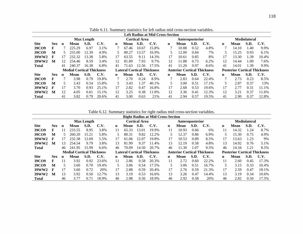
118

Table 6.11. Summary statistics for left radius mid cross-section variables. Left Radius at Mid Cross-Section

Max Length

Cortical Area

Anteroposterior

Mediolateral

Site Sex n Mean S.D. C.V. n Mean S.D. C.V. n Mean S.D. C.V. n Mean S.D. C.V.

39CO9 F 7 225.29 6.97 3.1% 7 67.46 10.67 15.8% 7 10.88 0.52 4.8% 7 14.10 1.40 9.9%

39CO9 M 5 255.00 12.39 4.9% 5 80.27 13.57 16.9% 5 12.00 0.84 7% 5 15.25 0.93 6.1%

39WW2 F 17 232.32 13.38 5.8% 17 63.55 9.11 14.3% 17 10.61 0.85 8% 17 13.30 1.39 10.4%

39WW2 M 12 254.46 8.59 3.4% 12 81.89 7.93 9.7% 12 11.88 0.73 6.2% 12 14.44 1.09 7.6%

Total 41 240.37 16.38 6.8% 41 71.63 12.56 17.5% 41 11.20 0.97 8.6% 41 14.01 1.39 9.9% Medial Cortical Thickness

Lateral Cortical Thickness

Anterior Cortical Thickness

Posterior Cortical Thickness

Site Sex n Mean S.D. C.V. n Mean S.D. C.V. n Mean S.D. C.V. n Mean S.D. C.V.

39CO9 F 7 3.98 0.79 19.8% 7 2.70 0.24 8.9% 7 2.83 0.64 22.4% 7 2.73 0.23 8.5%

39CO9 M 5 3.43 0.54 15.8% 5 3.43 1.37 40.1% 5 3.00 0.51 17.1% 5 2.87 0.37 13%

39WW2 F 17 3.70 0.93 25.1% 17 2.82 0.47 16.8% 17 2.68 0.53 19.6% 17 2.77 0.31 11.1%

39WW2 M 12 4.05 0.61 15.1% 12 3.25 0.38 11.8% 12 3.36 0.41 12.3% 12 3.21 0.37 11.6%

Total 41 3.82 0.79 20.6% 41 3.00 0.63 21% 41 2.94 0.57 19.5% 41 2.90 0.37 12.8%

Table 6.12. Summary statistics for right radius mid cross-section variables.

Right Radius at Mid Cross-Section Max Length

Cortical Area

Anteroposterior

Mediolateral

Site Sex n Mean S.D. C.V. n Mean S.D. C.V. n Mean S.D. C.V. n Mean S.D. C.V.

39CO9 F 11 233.55 8.95 3.8% 11 65.33 13.01 19.9% 11 10.93 0.66 6% 11 14.32 1.24 8.7%

39CO9 M 5 260.20 15.21 5.8% 5 80.31 9.82 12.2% 5 12.37 0.86 6.9% 5 15.30 0.75 4.9%

39WW2 F 17 232.38 12.69 5.5% 17 61.06 12.07 19.8% 17 10.53 0.89 8.5% 17 13.63 1.23 9%

39WW2 M 13 254.54 9.79 3.8% 13 81.99 9.37 11.4% 13 12.19 0.58 4.8% 13 14.92 0.76 5.1%

Total 46 241.95 15.99 6.6% 46 70.09 14.50 20.7% 46 11.30 1.07 9.5% 46 14.34 1.21 8.5% Medial Cortical Thickness

Lateral Cortical Thickness

Anterior Cortical Thickness

Posterior Cortical Thickness

Site Sex n Mean S.D. C.V. n Mean S.D. C.V. n Mean S.D. C.V. n Mean S.D. C.V.

39CO9 F 11 3.92 0.92 23.6% 11 2.86 0.58 20.3% 11 2.72 0.60 22.2% 11 2.60 0.45 17.3%

39CO9 M 5 3.60 0.70 19.4% 5 3.06 0.54 17.5% 5 3.06 0.51 16.7% 5 3.15 0.33 10.4%

39WW2 F 17 3.60 0.72 20% 17 2.88 0.59 20.4% 17 2.76 0.59 21.3% 17 2.59 0.47 18.1%

39WW2 M 13 3.92 0.50 12.7% 13 3.19 0.53 16.6% 13 3.26 0.47 14.4% 13 3.19 0.34 10.6%

Total 46 3.77 0.71 18.9% 46 2.98 0.56 18.9% 46 2.92 0.58 20% 46 2.82 0.50 17.5%

119

previous limb bone lengths. Unlike the humerus, mean cortical area is relatively similar for

right-side and left-side bones.

Females tend to exhibit more variation in right-side cross-sectional measurements. The

exception to this are the anteroposterior chords, where variation is greater for the males at the

Leavenworth site (39CO9). Left-side cross-sectional measurements tend to exhibit more

variation among the females at the Larson site (39WW2), but the pattern is more mixed at the

Leavenworth site.

Summary statistics for the ulna are presented in Table 6.13 (left-side) and Table 6.14

(right-side). The maximum length values are similar to those for the radius. Again, they exhibit

relatively low levels of variation in these samples. This seems to confirm that limb bone length

is relatively similar throughout the samples tested for this analysis.

The mean cortical area values are higher for are higher for right-side bones among the

male samples from both sites. The mean cortical area value for females is higher for the left-side

ulnae from the Leavenworth site (39CO9). The cortical area values are relatively equal for the

left-side among females from the Larson site (39WW2).

Barring a few measurements, females tend to exhibit more variation in most cross-

sectional measurements. The exceptions are left-side mediolateral chords and anterior cortical

thicknesses at the Leavenworth site (39CO9) and right-side medial cortical thickness and anterior

cortical thickness from the Larson site (39WW2), where males exhibit greater variation. Overall,

females from the Leavenworth site (39CO9), tend to have the most variation in ulna cross-

sectional variables.

120

Table 6.13. Summary statistics for left ulna mid cross-section variables. Left Ulna at Mid Cross-Section

Max Length

Cortical Area

Anteroposterior

Mediolateral

Site Sex n Mean S.D. C.V. n Mean S.D. C.V. n Mean S.D. C.V. n Mean S.D. C.V.

39CO9 F 5 250.20 11.34 4.5% 5 85.85 20.03 23.3% 5 15.05 1.62 10.8% 5 12.57 0.78 6.2%

39CO9 M 4 271.25 14.10 5.2% 4 91.80 15.05 16.4% 4 15.87 1.16 7.3% 4 13.30 1.24 9.3%

39WW2 F 14 250.54 14.73 5.9% 14 73.96 12.23 16.5% 14 14.28 1.52 10.7% 14 11.84 1.02 8.6%

39WW2 M 11 267.91 10.92 4.1% 11 91.64 12.99 14.2% 11 15.22 1.39 9.1% 11 13.15 1.18 9%

Total 34 258.54 15.55 6% 34 83.53 15.78 18.9% 34 14.89 1.50 10.1% 34 12.54 1.2 9.6% Medial Cortical Thickness

Lateral Cortical Thickness

Anterior Cortical Thickness

Posterior Cortical Thickness

Site Sex n Mean S.D. C.V. n Mean S.D. C.V. n Mean S.D. C.V. n Mean S.D. C.V.

39CO9 F 5 3.24 0.62 19.2% 5 3.22 0.99 30.7% 5 4.71 0.86 18.4% 5 3.16 1.01 32%

39CO9 M 4 3.19 0.35 11% 4 3.07 0.68 22.2% 4 4.40 1.14 25.9% 4 3.60 0.52 14.4%

39WW2 F 14 3.49 0.58 16.5% 14 3.07 0.69 22.4% 14 3.88 0.89 23.1% 14 3.26 0.48 14.7%

39WW2 M 11 3.83 0.37 9.6% 11 3.17 0.25 7.8% 11 3.62 0.69 19% 11 3.85 0.55 14.4%

Total 34 3.53 0.54 15.2% 34 3.12 0.61 19.4% 34 3.98 0.90 22.7% 34 3.47 0.64 18.5%

Table 6.14. Summary statistics for right ulna mid cross-section variables.

Right Ulna at Mid Cross-Section Max Length

Cortical Area

Anteroposterior

Mediolateral

Site Sex n Mean S.D. C.V. n Mean S.D. C.V. n Mean S.D. C.V. n Mean S.D. C.V.

39CO9 F 11 251.91 11.44 4.5% 11 75.58 19.83 26.2% 11 14.91 1.89 12.7% 11 12.42 1.48 11.9%

39CO9 M 5 278.20 14.31 5.1% 5 100.38 11.11 11.1% 5 16.38 0.70 4.3% 5 14.97 0.50 3.3%

39WW2 F 16 255.56 12.36 4.8% 16 74.32 12.06 16.2% 16 14.79 1.95 13.2% 16 12.12 1.05 8.7%

39WW2 M 15 271.73 11.90 4.4% 15 94.03 13.78 14.7% 15 16.18 1.35 8.4% 15 13.54 0.84 6.2%

Total 47 262.28 15.40 5.9% 47 83.68 17.69 21.1% 47 15.43 1.76 11.4% 47 12.95 1.39 10.7% Medial Cortical Thickness

Lateral Cortical Thickness

Anterior Cortical Thickness

Posterior Cortical Thickness

Site Sex n Mean S.D. C.V. n Mean S.D. C.V. n Mean S.D. C.V. n Mean S.D. C.V.

39CO9 F 11 3.11 0.76 24.4% 11 3.30 1.28 38.8% 11 4.20 1.25 29.7% 11 3.43 1.01 29.4%

39CO9 M 5 3.12 0.25 7.9% 5 4.86 1.64 33.6% 5 4.52 0.54 12% 5 3.71 0.51 13.8%

39WW2 F 16 2.88 0.48 16.5% 16 3.35 0.82 24.3% 16 3.64 0.99 27.1% 16 3.56 0.70 19.6%

39WW2 M 15 3.40 0.60 17.6% 15 3.35 0.57 16.9% 15 4.16 1.17 28.2% 15 4.07 0.62 15.1%

Total 47 3.13 0.60 19.2% 47 3.50 1.06 30.4% 47 4.03 1.09 27.1% 47 3.71 0.77 20.6%

121

Biological Distance and Correlation

Biological distance scores were developed using the Mahalanobis distance statistic

(Mahalanobis, 1936). Pairwise distance scores were calculated between groups using the

D2.dist() function from the biotools package in R (da Silva, 2015). The function relies on group

means and the pooled covariance matrix to calculate all possible pairwise distances within the

sample, resulting in a matrix containing the squared Mahalanobis distances (D2) between each

row of data and the center of each class of grouping (da Silva, 2015). The square root of these

scores (D) is presented here.

The Mahalanobis distance (D) matrices based on the raw, unadjusted variables are

presented in Table 6.15 (left-side) and Table 6.16 (right-side). The tables include a series of

distance matrices and the results of Mantel tests. The distance matrices were developed using

the variables listed in the summary statistics above. Distance matrices were calculated for each

cross-sectional locus. Each odontometric D matrix was created using variables from the same

individuals used to create the corresponding limb bone cross-sectional D matrix. If an individual

had to be deleted from the postcranial dataset due to incompleteness, they were also deleted from

the odontometric dataset for that analysis. To the right of each set of the D matrices in the table

are the results of the Mantel tests comparing their correlation.

Distances created from the postcranial datasets indicate that females from both sites tend

to be most similar to each other. The most noticeable departure from this trend is in the

subtrochanteric region, where females from Leavenworth site (39CO9) appear slightly more

similar to the males from Larson. The other postcranial distances and the distances created from

the odontometric data have a more mixed pattern indicating that biological sex alone is not the

only factor driving relationships in these datasets.

122

Table 6.15. Mahalanobis distance (D) for raw odontometrics and left-side cross-sections with Mantel results. Mahalanobis D from Left Side Bones Raw Data

Distances from Odontometrics

Distances from Femur Subtrochanteric Values

Mantel test 39CO9F 39CO9M 39WW2F 39WW2M

39CO9F 39CO9M 39WW2F 39WW2M

39CO9F 0.00 3.15 1.89 4.68 39CO9F 0.00 4.47 2.85 2.50 Permutation N: 9999

39CO9M 3.15 0.00 4.15 5.32 39CO9M 4.47 0.00 5.17 4.21 Correlation R: 0.051

39WW2F 1.89 4.15 0.00 5.37 39WW2F 2.85 5.17 0.00 3.09 p (uncorr; onetailed): 0.423

39WW2M 4.68 5.32 5.37 0.00 39WW2M 2.50 4.21 3.09 0.00

Distances from Odontometrics Distances from Femur Mid Values Mantel test 39CO9F 39CO9M 39WW2F 39WW2M

39CO9F 39CO9M 39WW2F 39WW2M

39CO9F 0.00 2.66 1.77 1.49 39CO9F 0.00 4.13 1.82 3.30 Permutation N: 9999

39CO9M 2.66 0.00 3.72 2.47 39CO9M 4.13 0.00 4.50 2.53 Correlation R: 0.691

39WW2F 1.77 3.72 0.00 2.12 39WW2F 1.82 4.50 0.00 3.23 p (uncorr; onetailed): 0.042

39WW2M 1.49 2.47 2.12 0.00 39WW2M 3.30 2.53 3.23 0.00

Distances from Odontometrics Distances from Tibia Mid Values Mantel test 39CO9F 39CO9M 39WW2F 39WW2M

39CO9F 39CO9M 39WW2F 39WW2M

39CO9F 0.00 2.92 2.42 1.93 39CO9F 0.00 4.04 1.91 4.30 Permutation N: 9999

39CO9M 2.92 0.00 3.37 1.86 39CO9M 4.04 0.00 4.30 2.54 Correlation R: 0.377

39WW2F 2.42 3.37 0.00 2.32 39WW2F 1.91 4.30 0.00 3.97 p (uncorr; onetailed): 0.254

39WW2M 1.93 1.86 2.32 0.00 39WW2M 4.30 2.54 3.97 0.00

Distances from Odontometrics Distances from Humerus Mid Values Mantel test 39CO9F 39CO9M 39WW2F 39WW2M

39CO9F 39CO9M 39WW2F 39WW2M

39CO9F 0.00 2.11 1.95 1.60 39CO9F 0.00 3.22 1.59 2.64 Permutation N: 9999

39CO9M 2.11 0.00 2.64 1.73 39CO9M 3.22 0.00 4.28 2.45 Correlation R: 0.739

39WW2F 1.95 2.64 0.00 2.05 39WW2F 1.59 4.28 0.00 3.38 p (uncorr; onetailed): 0.082

39WW2M 1.60 1.73 2.05 0.00 39WW2M 2.64 2.45 3.38 0.00

Distances from Odontometrics Distances from Radius Mid Values Mantel test 39CO9F 39CO9M 39WW2F 39WW2M

39CO9F 39CO9M 39WW2F 39WW2M

39CO9F 0.00 3.22 1.98 2.33 39CO9F 0.00 3.81 1.62 3.16 Permutation N: 9999

39CO9M 3.22 0.00 3.65 2.17 39CO9M 3.81 0.00 3.55 2.45 Correlation R: 0.826

39WW2F 1.98 3.65 0.00 2.67 39WW2F 1.62 3.55 0.00 2.66 p (uncorr; onetailed): 0.086

39WW2M 2.33 2.17 2.67 0.00 39WW2M 3.16 2.45 2.66 0.00

Distances from Odontometrics Distances from Ulna Mid Values Mantel test 39CO9F 39CO9M 39WW2F 39WW2M

39CO9F 39CO9M 39WW2F 39WW2M

39CO9F 0.00 1.75 1.98 1.10 39CO9F 0.00 2.77 1.68 3.39 Permutation N: 9999

39CO9M 1.75 0.00 3.15 2.02 39CO9M 2.77 0.00 3.07 2.56 Correlation R: -0.094

39WW2F 1.98 3.15 0.00 2.50 39WW2F 1.68 3.07 0.00 2.71 p (uncorr; onetailed): 0.717

39WW2M 1.10 2.02 2.50 0.00 39WW2M 3.39 2.56 2.71 0.00

123

Table 6.16. Mahalanobis distance (D) for raw odontometrics and right-side cross-sections with Mantel results. Mahalanobis D from Right Side Bones Raw Data

Distances from Odontometrics

Distances from Femur Subtrochanteric Values

Mantel test 39CO9F 39CO9M 39WW2F 39WW2M

39CO9F 39CO9M 39WW2F 39WW2M

39CO9F 0.00 2.39 1.47 2.02 39CO9F 0.00 3.97 3.36 3.43 Permutation N: 9999

39CO9M 2.39 0.00 2.97 2.88 39CO9M 3.97 0.00 5.22 4.54 Correlation R: 0.923

39WW2F 1.47 2.97 0.00 1.84 39WW2F 3.36 5.22 0.00 3.16 p (uncorr; onetailed): 0.042

39WW2M 2.02 2.88 1.84 0.00 39WW2M 3.43 4.54 3.16 0.00

Distances from Odontometrics Distances from Femur Mid Values Mantel test 39CO9F 39CO9M 39WW2F 39WW2M

39CO9F 39CO9M 39WW2F 39WW2M

39CO9F 0.00 2.71 1.88 1.82 39CO9F 0.00 4.68 2.74 4.02 Permutation N: 9999

39CO9M 2.71 0.00 3.70 2.76 39CO9M 4.68 0.00 6.10 4.35 Correlation R: 0.884

39WW2F 1.88 3.70 0.00 2.45 39WW2F 2.74 6.10 0.00 3.55 p (uncorr; onetailed): 0.042

39WW2M 1.82 2.76 2.45 0.00 39WW2M 4.02 4.35 3.55 0.00

Distances from Odontometrics Distances from Tibia Mid Values Mantel test 39CO9F 39CO9M 39WW2F 39WW2M

39CO9F 39CO9M 39WW2F 39WW2M

39CO9F 0.00 2.24 2.65 1.71 39CO9F 0.00 6.00 1.09 4.53 Permutation N: 9999

39CO9M 2.24 0.00 3.61 2.19 39CO9M 6.00 0.00 5.99 4.06 Correlation R: 0.139

39WW2F 2.65 3.61 0.00 2.60 39WW2F 1.09 5.99 0.00 3.96 p (uncorr; onetailed): 0.492

39WW2M 1.71 2.19 2.60 0.00 39WW2M 4.53 4.06 3.96 0.00

Distances from Odontometrics Distances from Humerus Mid Values Mantel test 39CO9F 39CO9M 39WW2F 39WW2M

39CO9F 39CO9M 39WW2F 39WW2M

39CO9F 0.00 2.39 1.72 1.25 39CO9F 0.00 3.21 1.54 2.36 Permutation N: 9999

39CO9M 2.39 0.00 2.93 2.10 39CO9M 3.21 0.00 4.31 2.58 Correlation R: 0.835

39WW2F 1.72 2.93 0.00 2.12 39WW2F 1.54 4.31 0.00 3.17 p (uncorr; onetailed): 0.045

39WW2M 1.25 2.10 2.12 0.00 39WW2M 2.36 2.58 3.17 0.00

Distances from Odontometrics Distances from Radius Mid Values Mantel test 39CO9F 39CO9M 39WW2F 39WW2M

39CO9F 39CO9M 39WW2F 39WW2M

39CO9F 0.00 2.67 1.49 2.23 39CO9F 0.00 3.29 1.04 2.84 Permutation N: 9999

39CO9M 2.67 0.00 2.69 1.69 39CO9M 3.29 0.00 3.59 1.02 Correlation R: 0.906

39WW2F 1.49 2.69 0.00 2.05 39WW2F 1.04 3.59 0.00 3.19 p (uncorr; onetailed): 0.131

39WW2M 2.23 1.69 2.05 0.00 39WW2M 2.84 1.02 3.19 0.00

Distances from Odontometrics Distances from Ulna Mid Values Mantel test 39CO9F 39CO9M 39WW2F 39WW2M

39CO9F 39CO9M 39WW2F 39WW2M

39CO9F 0.00 2.29 1.83 1.76 39CO9F 0.00 4.31 1.27 2.62 Permutation N: 9999

39CO9M 2.29 0.00 2.98 1.63 39CO9M 4.31 0.00 3.92 2.72 Correlation R: 0.538

39WW2F 1.83 2.98 0.00 2.45 39WW2F 1.27 3.92 0.00 2.20 p (uncorr; onetailed): 0.170

39WW2M 1.76 1.63 2.45 0.00 39WW2M 2.62 2.72 2.20 0.00

124

The Mantel results indicate that the distances created from the left-side cross-sectional

variables (Table 6.15) exhibit some correlation with those created from odontometric variables,

but the pattern is different for each bone. Significant (p<0.05) Mantel results are highlighted as

shaded rows. A moderate and significant correlation exists between distances created from

odontometric variables and those created from left femur midsection variables. Distances

created from the left humerus midsection and left radius midsection also have relatively high

correlation coefficients with p-values approaching significance.

For the right-side bones in Table 6.16, more loci exhibit significant correlations.

Distances created from variables at the subtrochanteric region and midsection of the femur along

with distances based on variables from the midsection of the humerus all exhibit relatively high

and statistically significant (p<0.05) correlations with distances created from odontometric

variables. Distances calculated from the radius and ulna also both exhibit moderate to high

correlations with the odontometric-based distances, but those correlations lack statistical

significance.

In order to account for differences in size, which may be less meaningful distinctions

between related individuals, the data were transformed and pairwise Mahalanobis distances (D)

were recalculated between groups. Cross-sectional variables were adjusted by bone length to

reflect the cortical dimensions relative to the size of the bone. Odontometric measurements were

size standardized by converting measurements to C-scores.

The pairwise D matrices along with the corresponding Mantel results for the size adjusted

datasets are presented in Table 6.17 (left-side) and Table 6.18 (right-side). Overall, the pattern is

similar to the one previously described for the Mahalanobis distance matrices constructed from

raw, unadjusted variables. Once again, the females from each site tend to be more similar in

125

Table 6.17. Mahalanobis distance (D) for size adjusted odontometrics and left-side cross-sections with Mantel results. Mahalanobis D from Left Side Bones Size Adjusted Data

Distances from Odontometrics

Distances from Femur Subtrochanteric Values

Mantel test 39CO9F 39CO9M 39WW2F 39WW2M

39CO9F 39CO9M 39WW2F 39WW2M

39CO9F 0.00 3.27 2.20 5.08 39CO9F 0.00 4.03 2.55 2.51 Permutation N: 9999

39CO9M 3.27 0.00 4.15 5.27 39CO9M 4.03 0.00 5.07 3.64 Correlation R: -0.021

39WW2F 2.20 4.15 0.00 5.23 39WW2F 2.55 5.07 0.00 2.77 p (uncorr; onetailed): 0.456

39WW2M 5.08 5.27 5.23 0.00 39WW2M 2.51 3.64 2.77 0.00

Distances from Odontometrics Distances from Femur Mid Values Mantel test 39CO9F 39CO9M 39WW2F 39WW2M

39CO9F 39CO9M 39WW2F 39WW2M

39CO9F 0.00 2.69 1.93 1.36 39CO9F 0.00 4.09 1.62 3.33 Permutation N: 9999

39CO9M 2.69 0.00 3.81 2.47 39CO9M 4.09 0.00 4.48 2.30 Correlation R: 0.593

39WW2F 1.93 3.81 0.00 2.27 39WW2F 1.62 4.48 0.00 3.09 p (uncorr; onetailed): 0.042

39WW2M 1.36 2.47 2.27 0.00 39WW2M 3.33 2.30 3.09 0.00

Distances from Odontometrics Distances from Tibia Mid Values Mantel test 39CO9F 39CO9M 39WW2F 39WW2M

39CO9F 39CO9M 39WW2F 39WW2M

39CO9F 0.00 2.66 2.47 1.65 39CO9F 0.00 3.83 1.95 4.17 Permutation N: 9999

39CO9M 2.66 0.00 3.38 1.85 39CO9M 3.83 0.00 4.17 2.43 Correlation R: 0.243

39WW2F 2.47 3.38 0.00 2.39 39WW2F 1.95 4.17 0.00 3.91 p (uncorr; onetailed): 0.290

39WW2M 1.65 1.85 2.39 0.00 39WW2M 4.17 2.43 3.91 0.00

Distances from Odontometrics Distances from Humerus Mid Values Mantel test 39CO9F 39CO9M 39WW2F 39WW2M

39CO9F 39CO9M 39WW2F 39WW2M

39CO9F 0.00 1.91 2.08 1.42 39CO9F 0.00 3.06 1.66 2.57 Permutation N: 9999

39CO9M 1.91 0.00 2.77 1.73 39CO9M 3.06 0.00 4.19 2.30 Correlation R: 0.655

39WW2F 2.08 2.77 0.00 2.19 39WW2F 1.66 4.19 0.00 3.38 p (uncorr; onetailed): 0.083

39WW2M 1.42 1.73 2.19 0.00 39WW2M 2.57 2.30 3.38 0.00

Distances from Odontometrics Distances from Radius Mid Values Mantel test 39CO9F 39CO9M 39WW2F 39WW2M

39CO9F 39CO9M 39WW2F 39WW2M

39CO9F 0.00 3.30 2.81 2.04 39CO9F 0.00 3.84 1.80 3.05 Permutation N: 9999

39CO9M 3.30 0.00 3.86 2.32 39CO9M 3.84 0.00 3.40 2.28 Correlation R: 0.403

39WW2F 2.81 3.86 0.00 3.09 39WW2F 1.80 3.40 0.00 2.19 p (uncorr; onetailed): 0.128

39WW2M 2.04 2.32 3.09 0.00 39WW2M 3.05 2.28 2.19 0.00

Distances from Odontometrics Distances from Ulna Mid Values Mantel test 39CO9F 39CO9M 39WW2F 39WW2M

39CO9F 39CO9M 39WW2F 39WW2M

39CO9F 0.00 1.75 2.32 1.16 39CO9F 0.00 1.57 1.86 3.07 Permutation N: 9999

39CO9M 1.75 0.00 3.27 2.04 39CO9M 1.57 0.00 2.24 2.21 Correlation R: -0.264

39WW2F 2.32 3.27 0.00 2.58 39WW2F 1.86 2.24 0.00 2.53 p (uncorr; onetailed): 0.631

39WW2M 1.16 2.04 2.58 0.00 39WW2M 3.07 2.21 2.53 0.00

126

Table 6.18. Mahalanobis distance (D) for size adjusted odontometrics and right-side cross-sections with Mantel results Mahalanobis D from Right Side Bones Size Adjusted Data

Distances from Odontometrics

Distances from Femur Subtrochanteric Values

Mantel test 39CO9F 39CO9M 39WW2F 39WW2M

39CO9F 39CO9M 39WW2F 39WW2M

39CO9F 0.00 2.58 1.87 1.47 39CO9F 0.00 3.80 3.31 3.39 Permutation N: 9999

39CO9M 2.58 0.00 2.96 2.63 39CO9M 3.80 0.00 4.95 4.24 Correlation R: 0.878

39WW2F 1.87 2.96 0.00 1.79 39WW2F 3.31 4.95 0.00 2.96 p (uncorr; onetailed): 0.041

39WW2M 1.47 2.63 1.79 0.00 39WW2M 3.39 4.24 2.96 0.00

Distances from Odontometrics Distances from Femur Mid Values Mantel test 39CO9F 39CO9M 39WW2F 39WW2M

39CO9F 39CO9M 39WW2F 39WW2M

39CO9F 0.00 2.74 2.11 1.69 39CO9F 0.00 4.71 2.81 3.85 Permutation N: 9999

39CO9M 2.74 0.00 3.84 2.75 39CO9M 4.71 0.00 6.11 4.00 Correlation R: 0.812

39WW2F 2.11 3.84 0.00 2.59 39WW2F 2.81 6.11 0.00 3.33 p (uncorr; onetailed): 0.044

39WW2M 1.69 2.75 2.59 0.00 39WW2M 3.85 4.00 3.33 0.00

Distances from Odontometrics Distances from Tibia Mid Values Mantel test 39CO9F 39CO9M 39WW2F 39WW2M

39CO9F 39CO9M 39WW2F 39WW2M

39CO9F 0.00 2.19 2.84 1.72 39CO9F 0.00 5.57 1.11 4.44 Permutation N: 9999

39CO9M 2.19 0.00 3.64 2.17 39CO9M 5.57 0.00 5.57 3.54 Correlation R: 0.025

39WW2F 2.84 3.64 0.00 2.68 39WW2F 1.11 5.57 0.00 3.91 p (uncorr; onetailed): 0.500

39WW2M 1.72 2.17 2.68 0.00 39WW2M 4.44 3.54 3.91 0.00

Distances from Odontometrics Distances from Humerus Mid Values Mantel test 39CO9F 39CO9M 39WW2F 39WW2M

39CO9F 39CO9M 39WW2F 39WW2M

39CO9F 0.00 2.15 1.69 1.25 39CO9F 0.00 2.90 1.62 2.29 Permutation N: 9999

39CO9M 2.15 0.00 2.95 2.15 39CO9M 2.90 0.00 4.10 2.38 Correlation R: 0.826

39WW2F 1.69 2.95 0.00 2.12 39WW2F 1.62 4.10 0.00 3.19 p (uncorr; onetailed): 0.040

39WW2M 1.25 2.15 2.12 0.00 39WW2M 2.29 2.38 3.19 0.00

Distances from Odontometrics Distances from Radius Mid Values Mantel test 39CO9F 39CO9M 39WW2F 39WW2M

39CO9F 39CO9M 39WW2F 39WW2M

39CO9F 0.00 2.38 1.62 1.87 39CO9F 0.00 2.64 1.02 2.34 Permutation N: 9999

39CO9M 2.38 0.00 2.74 1.71 39CO9M 2.64 0.00 2.70 0.92 Correlation R: 0.833

39WW2F 1.62 2.74 0.00 2.15 39WW2F 1.02 2.70 0.00 2.47 p (uncorr; onetailed): 0.037

39WW2M 1.87 1.71 2.15 0.00 39WW2M 2.34 0.92 2.47 0.00

Distances from Odontometrics Distances from Ulna Mid Values Mantel test 39CO9F 39CO9M 39WW2F 39WW2M

39CO9F 39CO9M 39WW2F 39WW2M

39CO9F 0.00 2.04 1.95 1.50 39CO9F 0.00 2.99 1.08 1.96 Permutation N: 9999

39CO9M 2.04 0.00 2.98 1.63 39CO9M 2.99 0.00 2.99 2.29 Correlation R: 0.396

39WW2F 1.95 2.98 0.00 2.46 39WW2F 1.08 2.99 0.00 1.87 p (uncorr; onetailed): 0.335

39WW2M 1.50 1.63 2.46 0.00 39WW2M 1.96 2.29 1.87 0.00

127

most cases.

The D matrices in Table 6.17 indicate a moderate and statistically significant (p<0.05)

correlation exists between Mahalanobis distances calculated from the femur midsection variables

and those calculated from odontometric variables. Again, the correlated cells are highlighted in

the table. There are also moderate but not significant correlations for the distances calculated

from the humerus and radius.

The right-side D matrices in Table 6.18 exhibit more significant correlations than the left-

side bones. Distances calculated from variables at the femur subtrochanteric region, the femur

midsection, the humerus midsection, and the radius midsection all exhibit relatively high and

significant (p<0.05) correlations with distances calculated from the corresponding odontometric

datasets.

To further explore the data, the sample was treated as a single group and intragroup

comparisons were conducted. Pairwise Mahalanobis distances (D2) were calculated using the

similarity and distance index in PAST v.3.09 (Hammer et al, 2001). The square root of these

distance scores (D) was used in this analysis. Due to the number of individuals in the analyses,

as many as 1,275 pairwise comparisons were created in each matrix. These D matrices are too

large to include in the results chapter and have been included as a separate appendix (Appendix

B).

The Mantel results comparing the intragroup pairwise D matrices are presented in Table

6.19. The table contains a series of Mantel results for comparisons between Mahalanobis

distance matrices calculated from odontometric variables and those constructed from the limb

bone cross-sectional variables. The pairwise D matrices (Appendix B) include distances

between all possible combinations of individuals in the sample. As with the intergroup distance

128

Table 6.19. Mantel results of intragroup pairwise Mahalanobis distance (D) matrices from odontometrics and cross-sections Mantel Results Based on Distances from Raw Variables Mantel Results Based on Distances from Size Adjusted Variables

Left Femur Subtrochanteric Right Femur Subtrochanteric Left Femur Subtrochanteric Right Femur Subtrochanteric

Mantel test

Mantel test

Mantel test

Mantel test

Permutation N: 9999 Permutation N: 9999 Permutation N: 9999 Permutation N: 9999

Correlation R: -0.083 Correlation R: -0.123 Correlation R: -0.062 Correlation R: -0.095

p (uncorr; onetailed): 0.760 p (uncorr; onetailed): 0.861 p (uncorr; onetailed): 0.692 p (uncorr; onetailed): 0.807

Left Femur Mid Right Femur Mid Left Femur Mid Right Femur Mid

Mantel test

Mantel test

Mantel test

Mantel test

Permutation N: 9999 Permutation N: 9999 Permutation N: 9999 Permutation N: 9999

Correlation R: -0.082 Correlation R: 0.018 Correlation R: -0.013 Correlation R: -0.021

p (uncorr; onetailed): 0.842 p (uncorr; onetailed): 0.422 p (uncorr; onetailed): 0.549 p (uncorr; onetailed): 0.565

Left Tibia Mid Right Tibia Mid Left Tibia Mid Right Tibia Mid

Mantel test

Mantel test

Mantel test

Mantel test

Permutation N: 9999 Permutation N: 9999 Permutation N: 9999 Permutation N: 9999

Correlation R: -0.041 Correlation R: 0.002 Correlation R: 0.003 Correlation R: -0.004

p (uncorr; onetailed): 0.672 p (uncorr; onetailed): 0.475 p (uncorr; onetailed): 0.459 p (uncorr; onetailed): 0.505

Left Humerus Mid Right Humerus Mid Left Humerus Mid Right Humerus Mid

Mantel test

Mantel test

Mantel test

Mantel test

Permutation N: 9999 Permutation N: 9999 Permutation N: 9999 Permutation N: 9999

Correlation R: 0.195 Correlation R: 0.061 Correlation R: 0.188 Correlation R: 0.074

p (uncorr; onetailed): 0.017 p (uncorr; onetailed): 0.263 p (uncorr; onetailed): 0.025 p (uncorr; onetailed): 0.242

Left Radius Mid Right Radius Mid Left Radius Mid Right Radius Mid

Mantel test

Mantel test

Mantel test

Mantel test

Permutation N: 9999 Permutation N: 9999 Permutation N: 9999 Permutation N: 9999

Correlation R: -0.130 Correlation R: 0.107 Correlation R: -0.105 Correlation R: 0.207

p (uncorr; onetailed): 0.869 p (uncorr; onetailed): 0.150 p (uncorr; onetailed): 0.828 p (uncorr; onetailed): 0.024

Left Ulna Mid Right Ulna Mid Left Ulna Mid Right Ulna Mid

Mantel test

Mantel test

Mantel test

Mantel test

Permutation N: 9999 Permutation N: 9999 Permutation N: 9999 Permutation N: 9999

Correlation R: 0.126 Correlation R: 0.092 Correlation R: 0.150 Correlation R: 0.176

p (uncorr; onetailed): 0.131 p (uncorr; onetailed): 0.160 p (uncorr; onetailed): 0.095 p (uncorr; onetailed): 0.035

129

scores, I have included distance calculated from both raw variables and the size-adjusted

variables in the table. The Mantel results have been separated by the bone cross-section used in

the analysis, with the comparisons of the raw unadjusted datasets on the left of the table and the

size adjusted comparisons on the right. Significant correlations (p<.05) have been highlighted.

The correlation coefficients are low for all of the Mantel results presented in Table 6.19.

For the Mantel results based on the raw dataset (left half of Table 6.19), only the distances

constructed from left humerus cross-sectional variables exhibit a significant correlation (p<0.05)

with odontometric-based distances. Mantel results comparing the D matrices constructed from

size adjusted variables are also presented in Table 6.19. Like the results for distances created

from the raw variables, there is a significant correlation (p<0.05) between D matrices constructed

from size-adjusted left side humerus midsection variables and those constructed from

standardized odontometric variables. In addition, D matrices created from right-side radius and

ulna midsection variables exhibit significant correlations with those constructed from

standardized odontometric variables. The comparison between size adjusted left ulna and

standardized odontometric variables is approaching statistical significance with a p-value of

0.095.

A number of the other correlation coefficients in Table 6.19 indicate low correlations in

the same range as those listed above. However, none of these are statistically significant. For

example, the comparison of D matrices for the size-adjusted left ulna approaches significance

with a correlation of 0.150 and a p-value of .095. The femur and tibia depart from this trend

towards slight correlations with each bone exhibiting low, non-significant results.

Similar to the intergroup comparisons, the Mantel results comparing the intragroup

distance matrices indicate that size adjusted variables produce more significant correlations than

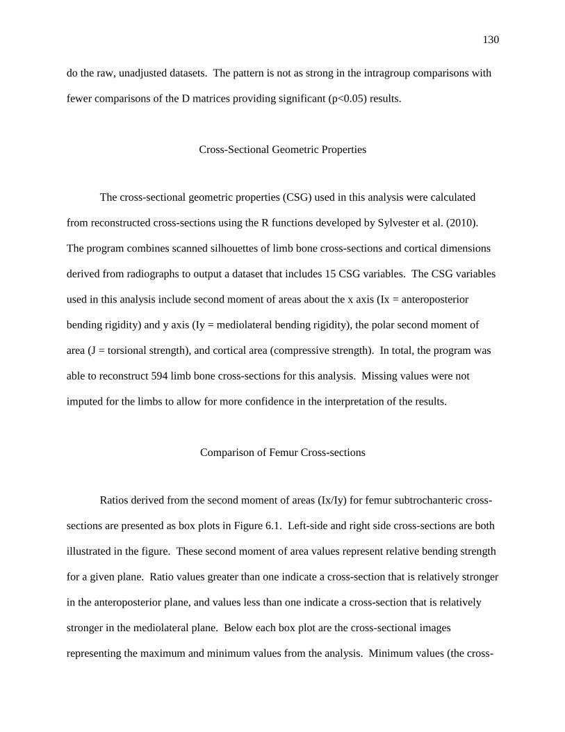
130

do the raw, unadjusted datasets. The pattern is not as strong in the intragroup comparisons with

fewer comparisons of the D matrices providing significant (p<0.05) results.

Cross-Sectional Geometric Properties

The cross-sectional geometric properties (CSG) used in this analysis were calculated

from reconstructed cross-sections using the R functions developed by Sylvester et al. (2010).

The program combines scanned silhouettes of limb bone cross-sections and cortical dimensions

derived from radiographs to output a dataset that includes 15 CSG variables. The CSG variables

used in this analysis include second moment of areas about the x axis (Ix = anteroposterior

bending rigidity) and y axis (Iy = mediolateral bending rigidity), the polar second moment of

area (J = torsional strength), and cortical area (compressive strength). In total, the program was

able to reconstruct 594 limb bone cross-sections for this analysis. Missing values were not

imputed for the limbs to allow for more confidence in the interpretation of the results.

Comparison of Femur Cross-sections

Ratios derived from the second moment of areas (Ix/Iy) for femur subtrochanteric cross-

sections are presented as box plots in Figure 6.1. Left-side and right side cross-sections are both

illustrated in the figure. These second moment of area values represent relative bending strength

for a given plane. Ratio values greater than one indicate a cross-section that is relatively stronger

in the anteroposterior plane, and values less than one indicate a cross-section that is relatively

stronger in the mediolateral plane. Below each box plot are the cross-sectional images

representing the maximum and minimum values from the analysis. Minimum values (the cross-

131

Figure 6.1. Box plots of Ix/Iy ratios for left and right femur subtrochanteric cross-sections. Images for

maximum and minimum values are presented below the box plots.

132

sectional images on the left below each set of box plots) are wider with more cortical bone

deposited in the mediolateral dimension. In contrast, the images representing cross-sections with

maximum ratio values (the images on the right below each set of box plots) are elongated in the

anteroposterior plane with more cortical bone positioned in those areas.

A few patterns are apparent from the illustration. Right-side subtrochanteric cross-

sections exhibit more variation than left-side cross-sections in this sample and on average have

higher ratio values, which indicates that right side bones are more likely to have greater bending

strength in the anteroposterior dimension. Females from both sites are more variable than men

indicating more variation in bending strength among females in general. Right-side cross-

sections from females at the Leavenworth site (39CO9) exhibit the most variation and have the

highest ratios in the sample.

An ANOVA was performed to determine if the ratio values differ significantly between

the groups. The results of the ANOVA for left femur subtrochanteric Ix/Iy ratios are presented

in Table 6.20. There is a significant difference (p<.05) in mean values of the groups. Tukey’s

pairwise comparisons in Table 6.21 indicate that, despite a significant overall difference between

the groups, no pairwise tests were significant. The pairwise comparison between males and

females at the Leavenworth site (39CO9) approaches significance with a p-value of 0.0633 for

the left-side subtrochanteric cross-sections.

The result of the ANOVA comparing right-side subtrochanteric Ix/Iy ratios are presented

in Table 6.22. The right-side mean values do not differ significantly in these groups, but the p-

value of 0.07291 indicates the results are approaching statistical significance (p<0.05). The

Tukey’s pairwise comparisons in Table 6.23 indicate that no significant pairwise differences are

present in this sample for right-side ratios.

133

Table 6.20. ANOVA results for left femur subtrochanteric Ix/Iy ratio.

Test for equal means for left femur subtrochanteric Ix/Iy ratio

Sum of sqrs df Mean square F p (same)

Between groups: 0.207948 3 0.0693161 3.975 0.01694

Within groups: 0.523193 30 0.0174398

Total: 0.731141 33

Table 6.21. Tukey’s pairwise for left femur subtrochanteric Ix/Iy ratio (p-values in upper right). 39CO9F 39CO9M 39WW2F 39WW2M

39CO9F

0.0633 0.432 0.248

39CO9M 3.694

0.7039 0.893

39WW2F 2.166 1.528

0.982

39WW2M 2.691 1.003 0.5254

Table 6.22. ANOVA results for right femur subtrochanteric Ix/Iy ratio.

Test for equal means for right femur subtrochanteric Ix/Iy ratio Sum of sqrs df Mean square F p (same)

Between groups: 0.667023 3 0.222341 2.52 0.07291

Within groups: 3.2651 37 0.0882458

Total: 3.93212 40

Table 6.23. Tukey’s pairwise for right femur subtrochanteric Ix/Iy ratio (p-values in upper right). 39CO9F 39CO9M 39WW2F 39WW2M

39CO9F

0.6248 0.2097 0.448

39CO9M 1.711

0.8623 0.991

39WW2F 2.816 1.106

0.961

39WW2M 2.122 0.4109 0.6947

134

To further explore the variation in subtrochanteric Ix/Iy ratios, absolute asymmetry was

calculated using right and left values. This percentage score indicates the magnitude of

asymmetry within an individual regardless of side bias. Box plots of the percent of absolute

asymmetry for the ratios are presented in Figure 6.2. To the right of the box plots are the cross-

sectional images for the most asymmetrical (top cross-sectional silhouettes) and least

asymmetrical (bottom cross-sectional silhouettes) individuals in the sample. Females from the

Leavenworth site (39CO9) exhibit the most variation and the highest percentage of asymmetry in

the subtrochanteric Ix/Iy ratios. The cross-sectional silhouettes for the maximum percentage of

absolute asymmetry illustrate that relative to the left-side subtrochanteric region, the right-side

subtrochanteric region for the female from Leavenworth (39CO9F_F102_B2A) is more

elongated in the anteroposterior dimension with more cortical bone deposited along that plane.

In contrast, the least asymmetrical individual in Figure 6.2 is the male from the Larson site

(39WW2M_F201_B54B) who exhibits similar cross-sections.

The results of the ANOVA on the values for percent absolute asymmetry in the

subtrochanteric Ix/Iy ratios are presented in Table 6.24. Males from Larson (39WW2) were only

represented by a single individual (due to only one male having both right and left bones) and

were not included in the ANOVA. The results indicate a significant difference (p<.05) exists

between the means of the groups included in the analysis. Confirming the significance of the

pattern noted in the box plots, the Tukey’s pairwise results in Table 6.25 indicate that females

from the Leavenworth site are significantly different from the other groups.

Absolute asymmetry was also calculated for the polar second moment of area (J) in these

samples. The polar second moment of area indicates the relative torsional strength of a cross-

section, and asymmetry in these measures indicates a difference in the ability of right and left-

135

Figure 6.2. Box plots of femur subtrochanteric Ix/Iy ratio values for percentage of absolute asymmetry by

group. The images to the right of the box plots are left and right subtrochanteric cross-sections for

maximum (above) and minimum (below) values.

Table 6.24. ANOVA results for right subtrochanteric Ix/Iy ratio percent absolute asymmetry.

Test for equal means for femur subtrochanteric Ix/Iy ratio % absolute asymmetry

Sum of sqrs df Mean square F p (same)

Between groups: 6800.32 2 3400.16 8.105 0.001935

Within groups: 10487.5 25 419.501

Total: 17287.8 27

Table 6.25. Tukey’s pairwise for femur subtrochanteric Ix/Iy ratio percent absolute asymmetry. (p-values

in upper right). 39CO9F 39CO9M 39WW2F

39CO9F

0.007821* 0.03913*

39CO9M 4.679

0.7642

39WW2F 3.686 0.9938

136

side cross-sections to resist torsional stress. Box plots of the absolute asymmetry values for J at

the subtrochanteric region are illustrated in Figure 6.3. All of the groups, with the exception of

the single male from Larson (39WW2), exhibit considerable variation in the asymmetry of J.

The most asymmetrical subtrochanteric cross-section, which is illustrated to the right of the box

plot, is from a female from the Leavenworth site (39CO9). The cross-sections from that the

right-side subtrochanteric region has considerably thinner cortices than the left-side.

The results of the ANOVA comparing the mean values for absolute asymmetry in the

polar second moment of area are presented in Table 6.26. Again, the males from the Larson site

were not included in the analysis due to the small sample. The ANOVA indicates that there is no

significant difference in the asymmetry in torsional strength for these groups. The Tukey’s

pairwise comparison in Table 6.27 supports this finding, with no significant differences between

any of the groups.

Cortical area is understood to reflect resistance to compressive forces in a limb bone

cross-section. For interpretive purposes, Ruff (2008) recommends adjusting the measurement by

bone length3 to account for the allometric relationship between cortical development and the size

of the individual. Size adjusted subtrochanteric cortical areas for left and right-side bones are

presented as box plots in Figure 6.4. Below each box plot, a pair of images representing the

maximum and minimum cross-sectional values has been included.

For both right-side and left-side cortical area, females exhibit more variation at each site.

The least robust cortical value for the left-side subtrochanteric region belongs to a female from

the Larson site (39WW2) and the most robust left-side subtrochanteric cortical value belongs to a

female from the Leavenworth site (39CO9). In contrast, the most robust right-side

subtrochanteric cortical value belongs to a male from the Larson site and the least robust value

137

Figure 6.3. Box plots of femur subtrochanteric J values for percentage of absolute asymmetry by group.

The images to the right of the box plots are left and right subtrochanteric cross-sections for maximum

(above) and minimum (below) values.

Table 6.26. ANOVA results for femur subtrochanteric J percent absolute asymmetry.

Test for equal means for femur subtrochanteric J % absolute asymmetry

Sum of sqrs df Mean square F p (same)

Between groups: 628.415 2 314.208 1.27 0.2984

Within groups: 6186 25 247.44

Total: 6814.42 27

Table 6.27. Tukey’s pairwise for femur subtrochanteric J percent absolute asymmetry. (p-values in the

upper right) 39CO9F 39CO9M 39WW2F

39CO9F

0.8169 0.5854

39CO9M 0.8606

0.2619

39WW2F 1.41 2.271

138

Figure 6.4. Box plots of size adjusted cortical areas for left and right femur subtrochanteric cross-sections.

Images for maximum and minimum values are presented below the box plots.

139

belongs to a female from the Leavenworth site. Visual inspection of the box plots indicates that

mean values for males tend to be higher in these samples and the right-side mean values for

males at the Larson site (39WW2) stand out as the highest in the sample.

The results of an ANOVA comparing the left-side size adjusted cortical values for the

subtrochanteric region is presented in Table 6.28. The results indicate that there are no

significant differences between the mean values of these samples. The Tukey’s pairwise

comparisons for the left side are consistent with the ANOVA results (Table 6.29).

Right-side size adjusted cortical values do differ significantly between these groups for

the subtrochanteric region. The result of the ANOVA is presented in Table 6.30. The mean

values are significantly different between the groups (p<0.05). An inspection of the box plots in

Figure 6.4 suggests that the males from the Larson site (39WW2) are the most different in these

values. The Tukey’s pairwise comparisons in Table 6.31 indicate there are no significant

(p<0.05) pairwise differences, however, the difference between the males from each site is

approaching significance with a p-value of 0.06.

Asymmetry in cortical area reflects a relative difference in resistance to compressive

forces between the left and right-side of the body. The box plots in Figure 6.5 illustrate the

percentage of absolute asymmetry for the cortical area at the subtrochanteric region for

individuals in the sample divided by sex and group. The cross-sectional images to the right of

the box plots are right-side and left-side cross-sectional reconstructions for the maximum (the

upper two images) and minimum (the lower two images) values from the analysis.

The box plots indicate that females at each site exhibit more variation in the cortical area

asymmetry in this region than do their male counterparts. It should be noted, however that males

from the Larson site (39WW2) are only represented by one individual for the subtrochanteric

140

Table 6.28. ANOVA results for left femur subtrochanteric size adjusted cortical areas.

Test for equal means for left femur subtrochanteric cortical area

Sum of sqrs df Mean square F p (same)

Between groups: 1.30E-12 3 4.34E-13 0.7485 0.5321

Within groups: 1.68E-11 29 5.79E-13

Total: 1.81E-11 32

Table 6.29. Tukey’s pairwise for left femur subtrochanteric size adjusted cortical areas. (p-values in the

upper right) 39CO9F 39CO9M 39WW2F 39WW2M

39CO9F

0.9859 0.8652 0.9754

39CO9M 0.4847

0.6819 0.9999

39WW2F 1.096 1.581

0.6376

39WW2M 0.5879 0.1032 1.684

Table 6.30. ANOVA results for right femur subtrochanteric size adjusted cortical areas.

Test for equal means for right femur subtrochanteric cortical area

Sum of sqrs df Mean square F p (same)

Between groups: 7.08E-12 3 2.36E-12 3.534 0.0256

Within groups: 2.14E-11 32 6.68E-13

Total: 2.84E-11 35

Table 6.31. Tukey’s pairwise for right femur subtrochanteric size adjusted cortical areas. (p-values in the

upper right) 39CO9F 39CO9M 39WW2F 39WW2M

39CO9F

1 0.9608 0.06082

39CO9M 0.001352

0.9606 0.0607

39WW2F 0.693 0.6944

0.1649

39WW2M 3.708 3.71 3.015

141

Figure 6.5. Box plots of femur subtrochanteric cortical area for percentage of absolute asymmetry by

group. The images to the right of the box plots are left and right subtrochanteric cross-sections for

maximum (above) and minimum (below) values.

Table 6.32. ANOVA results for femur subtrochanteric cortical area percent absolute asymmetry.

Test for equal means for femur subtrochanteric cortical area % absolute asymmetry

Sum of sqrs df Mean square F p (same)

Between groups: 512.182 2 256.091 0.9542 0.3987

Within groups: 6709.71 25 268.388

Total: 7221.89 27

Table 6.33. Tukey’s pairwise for femur subtrochanteric cortical area percent absolute asymmetry. (p-

values in the upper right) 39CO9F 39CO9M 39WW2F

39CO9F

0.9883 0.5397

39CO9M 0.2075

0.6296

39WW2F 1.516 1.309

142

region. Females from the Leavenworth site (39CO9) have on average slightly greater asymmetry

and more variation overall than do females from the Larson site.

The differences between the means of these groups, however, are not significant

according to the results of the ANOVA presented in Table 6.32. This result is supported by the

pairwise comparisons in Table 6.33, which also indicate that no significant differences were

found between the groups in the percentage of absolute asymmetry in cortical area at this locus.

Again, it should be noted that the ANOVA and Tukey’s comparisons exclude the single male

that was recorded from the Larson sample. Overall, these results indicate that while there is

considerable asymmetry in the amount of cortical bone among some individuals in this sample,

the difference in that asymmetry is not significant at the group level.

Ratios derived from the second moment of areas (Ix/Iy) for femur midsection cross-

sections are presented as box plots in Figure 6.6. Again, as with the subtrochanteric region, these

values represent relative bending strength at this locus. The ratios for left-side cross-sections are

presented on the left half of the figure with images of the minimum and maximum ratio values

presented under the box plots. The right-side values are illustrated on the right hand side of the

figure.

The box plots indicate that for both the right and left side, the second moment of area

ratios are slightly greater on average for males at both sites with males having more individuals

with ratios falling above 1. This indicates that at both sites males are more likely to have cross-

sections that have greater resistance to bending force in the anteroposterior dimension in the

middle of the femur. The box plots also indicate that females are more variable in these ratios at

each site on both the right and left-sides.

143

Figure 6.6. Box plots of Ix/Iy ratios for left and right femur mid cross-sections. Images for maximum and

minimum values are presented below the box plots.

144

Table 6.34. ANOVA results for left femur mid Ix/Iy ratio.

Test for equal means for left femur mid Ix/Iy ratio

Sum of sqrs df Mean square F p (same)

Between groups: 0.214527 3 0.071509 1.83 0.1532

Within groups: 2.0324 52 0.039085

Total: 2.24692 55

Table 6.35. Tukey’s pairwise for left femur mid Ix/Iy ratio. (p-values in the upper right). 39CO9F 39CO9M 39WW2F 39WW2M

39CO9F

0.5769 0.9963 0.5169

39CO9M 1.816

0.4431 0.9997

39WW2F 0.3092 2.126

0.3879

39WW2M 1.953 0.1366 2.262

Table 6.36. ANOVA results for right femur mid Ix/Iy ratio.

Test for equal means for right femur mid Ix/Iy ratio

Sum of sqrs df Mean square F p (same)

Between groups: 0.294206 3 0.098069 2.31 0.0873

Within groups: 2.16503 51 0.042452

Total: 2.45924 54

Table 6.37. Tukey’s pairwise for right femur mid Ix/Iy ratio. (p-values in the upper right). 39CO9F 39CO9M 39WW2F 39WW2M

39CO9F

0.3568 0.9195 0.7696

39CO9M 2.343

0.1128 0.8999

39WW2F 0.9014 3.245

0.3863

39WW2M 1.365 0.9781 2.267

145

ANOVA results for Ix/Iy ratios at the femur midsection indicate that there are no

significant differences between the groups for either side. Table 6.34 indicates that left-side

ratios are not significantly different (p<0.05) between any of the four groups used in the analysis.

This is supported by the Tukey’s pairwise comparisons in Table 6.35. The ANOVA results in

Table 6.36 also indicate no significant difference, however, the p-value of 0.08 is approaching

significance. An examination of the box plots indicates that differences between males and

females, especially males from the Leavenworth site (39CO9), are likely driving any difference

seen in the results. The Tukey’s pairwise comparisons in Table 6.37 support the results of the

ANOVA for the right-side bones, and the lower p-values for the male-female comparisons seems

to support the interpretation that sex differences are the most meaningful.

Values for absolute asymmetry in Ix/Iy ratios at the femur mid cross-section are

presented as box plots in Figure 6.7. In the figure, the cross-sectional images to the right of the

box plots represent the left and right-side bones from the most asymmetrical (top) and least

asymmetrical (bottom) individuals in the sample. Barring a few exceptions, the box plot in

Figure 6.7 illustrates a relatively low level of absolute asymmetry when compared to the same

values for the subtrochanteric region (Figure 6.2) in these groups. Females tend to exhibit a

wider range of asymmetry in each group and males from the Leavenworth site (39CO9) have the

highest average values among the samples.

The ANOVA in Table 6.38 indicates there are no significant differences (p<0.05)

between the groups in this analysis. The Tukey’s pairwise analysis in Table 6.39 is consistent

with this result. Overall, asymmetry in bending strength at the femur midsection does not

distinguish these groups.

146

Figure 6.7. Box plots of femur mid Ix/Iy ratio values for percentage of absolute asymmetry by group.

The images to the right of the box plots are left and right subtrochanteric cross-sections for maximum

(above) and minimum (below) values.

Table 6.38. ANOVA results for femur mid Ix/Iy ratio percent absolute asymmetry.

Test for equal means for femur mid Ix/Iy ratio % absolute asymmetry

Sum of sqrs df Mean square F p (same)

Between groups: 283.15 3 94.3832 1.126 0.3479

Within groups: 4022.94 48 83.8113

Total: 4306.09 51

Table 6.39. Tukey’s pairwise for femur mid Ix/Iy ratio percent absolute asymmetry. (p-values in the upper

right) 39CO9F 39CO9M 39WW2F 39WW2M

39CO9F

0.988 0.9987 0.7066

39CO9M 0.4606

0.9983 0.5054

39WW2F 0.219 0.2416

0.6116

39WW2M 1.52 1.98 1.739

147

Figure 6.8. Box plots of femur mid J for percentage of absolute asymmetry by group. The images to the

right of the box plots are left and right subtrochanteric cross-sections for maximum (above) and minimum

(below) values.

Table 6.40. ANOVA results for femur mid J percent absolute asymmetry.

Test for equal means for femur mid J % absolute asymmetry

Sum of sqrs df Mean square F p (same)

Between groups: 3802.91 3 1267.64 12.48 3.73E-06

Within groups: 4875.9 48 101.581

Total: 8678.81 51

Table 6.41. Tukey’s pairwise for femur mid J percent absolute asymmetry. (p-values in the upper right) 39CO9F 39CO9M 39WW2F 39WW2M

39CO9F

0.0002687* 0.001693* 0.002179*

39CO9M 6.686

0.8483 0.8042

39WW2F 5.537 1.149

0.9998

39WW2M 5.411 1.275 0.1257

148

Box plots illustrating the percentage of absolute asymmetry in torsional strength (J) are

presented in Figure 6.8. There is a marked difference in the asymmetry of J between the females

from the Leavenworth site (39CO9) and the other groups. The females from Leavenworth

exhibit much higher mean values and a greater range of variation in the asymmetry of J at the

femur midsection when compared to the other groups.

The ANOVA presented in Table 6.40 indicates that the difference between these groups

is highly significant. The Tukey’s pairwise comparisons in Table 6.41 indicate that the

significance of the ANOVA is driven entirely by the females from the Leavenworth site with that

group exhibiting significant differences from each of the other three groups in this analysis. The

females from the Leavenworth site have much higher levels of asymmetry in torsional strength

than do any of the individuals from the other groups, including males from the same site.

Box plots illustrating the cortical area adjusted by bone length at the midsection of the

femur are presented in Figure 6.9. Left-side and right-side bones are separated in the figure with

cross-sectional images representing the minimum and maximum in the analysis below each box

plot. For both the left and right side bone, females exhibit more variation than males in cortical

area at the femur midshaft. Although females exhibit more variation and in some cases have the

highest values, the average amount of cortical bone tends to be higher among males. In addition,

right-side values tend to be higher than left-side values for all groups, indicating that right-side

bones tend to have more cortical bone.

The ANOVA presented in Table 6.42 indicates that cortical area does not significantly

differ (p<0.05) among these groups for left-side bones. The Tukey’s pairwise comparisons for

left-side cortical area at the femur midshaft in Table 6.43 support the finding in the ANOVA. In

contrast to the left-side, the ANOVA results in Table 6.44 indicate there is a significant

149

Figure 6.9. Box plots of size adjusted cortical areas for left and right femur mid cross-sections. Images

for maximum and minimum values are presented below the box plots.

150

Table 6.42. ANOVA results for left femur mid size adjusted cortical areas.

Test for equal means for left femur mid cortical area

Sum of sqrs df Mean square F p (same)

Between groups: 2.20E-12 3 7.35E-13 1.508 0.2245

Within groups: 2.34E-11 48 4.88E-13

Total: 2.56E-11 51

Table 6.43. Tukey’s pairwise for left femur mid size adjusted cortical areas. (p-values in upper right) 39CO9F 39CO9M 39WW2F 39WW2M

39CO9F

0.8865 0.9999 0.416

39CO9M 1.026

0.9089 0.8422

39WW2F 0.08228 0.9439

0.4498

39WW2M 2.193 1.167 2.111

Table 6.44. ANOVA results for right femur mid size adjusted cortical areas.

Test for equal means for right femur mid cortical area

Sum of sqrs df Mean square F p (same)

Between groups: 8.36E-12 3 2.79E-12 8.783 0.000112

Within groups: 1.40E-11 44 3.17E-13

Total: 2.23E-11 47

Table 6.45. Tukey’s pairwise for right femur mid size adjusted cortical areas. (p-values in upper right). 39CO9F 39CO9M 39WW2F 39WW2M

39CO9F

0.155 0.3766 0.001321*

39CO9M 3.034

0.9533 0.248

39WW2F 2.295 0.7386

0.08999

39WW2M 5.704 2.67 3.409

151

difference between the right-side mean cortical areas for these groups. The Tukey’s pairwise

comparisons in Table 6.45 indicates the most significant difference on right-side is between

males from the Larson site (39WW2) and females from the Leavenworth site (39CO9).

Box plots illustrating the amount of absolute asymmetry in cortical area by group are

presented in Figure 6.10. Cross-sectional images of right-side and left-side bones for the most

asymmetrical (top two cross-sectional images) and least asymmetrical (bottom two cross-

sectional images) individuals in the analysis are presented to the right of the box plots. Upon

visual inspection of these images, it is apparent that, although asymmetry exists to varying

degrees in cortical area at the femur midsection, right-side and left-side cross-sections are rather

similar. Females from the Leavenworth site (39CO9) exhibit much more variation and have

higher values of asymmetry than all other groups. The maximum value for absolute asymmetry

is from a female from the Leavenworth site with an asymmetry in cortical area at the femur

midsection approaching 30%. The individual who exhibited the least asymmetry was a female

from the Larson site (39WW2).

The results of the ANOVA conducted on the absolute asymmetry data for the cortical

area at the femur midsection are presented in Table 6.46. The analysis indicates a highly

significant (p<0.0001) difference between these groups. The Tukey’s pairwise comparisons in

Table 6.47 confirm what is visually evident in the box plots. Specifically, the differences

between the females from the Leavenworth site (39CO9) and all other groups are the most

notable. The p-values in Table 6.47 indicate that the most significant difference exists between

males and females at the Leavenworth site. Males and females at the Larson site are much more

similar in the asymmetry they exhibit in cortical area at the femur midsection.

152

Figure 6.10. Box plots of femur mid cortical area for percentage of absolute asymmetry by group. The

images to the right of the box plots are left and right subtrochanteric cross-sections for maximum (above)

and minimum (below) values.

Table 6.46. ANOVA results for femur mid cortical area percent absolute asymmetry.

Test for equal means for femur mid cortical area % absolute asymmetry

Sum of sqrs df Mean square F p (same)

Between groups: 967.296 3 322.432 8.948 8.16E-05

Within groups: 1729.66 48 36.0346

Total: 2696.96 51

Table 6.47. Tukey’s pairwise for femur mid cortical area percent absolute asymmetry.(p-values in upper

right). 39CO9F 39CO9M 39WW2F 39WW2M

39CO9F

0.0004213* 0.009837* 0.02385*

39CO9M 6.312

0.6489 0.4445

39WW2F 4.658 1.654

0.9873

39WW2M 4.188 2.124 0.47

153

Comparison of Tibia Cross-sections

Ratios derived from the second moment of areas at the tibia midshaft are presented as

box plots in Figure 6.11. Left and right-side bones are separated in the figure with images from

the minimum and maximum ratios under each series of plots. Nearly all of the individuals

exhibit ratios that are above a value of 1, which indicates greater resistance to bending strength

in the anteroposterior dimension. For left-side tibia, Ix/Iy ratios exhibit noticeably more

variation among individuals from the Larson site (39WW2). The males from Larson also exhibit

much greater variation on the right-side than do the other groups. With the exception of right-

side tibia from the Leavenworth site, males exhibit higher ratios on average than females. Again,

these higher ratios indicate a tibia cross-section that is stronger in the anteroposterior dimension.

The cross-sectional images representing individuals with maximum values illustrate that these

tibia are narrow with considerable cortical bone deposited along the anterior margin.

The ANOVA results from the comparison of left-side Ix/Iy ratios at the tibia midsection

are presented in Table 6.48. The results indicate that the groups presented here are significantly

different (p<0.05) from each other. The Tukey’s pairwise comparisons in Table 6.49 indicate

that the most significant difference for the left tibia is between the males form the Larson site

(39WW2) and the females from the Leavenworth site (39CO9). The difference between the

males from each site is also approaching significance with a p-value of 0.08.

The right-side results also indicate significant differences exist between these groups for

the Ix/Iy ratios in the tibia. The ANOVA results presented in Table 6.50 indicate the differences

between the means of these groups are highly significant. According to the Tukey’s pairwise

comparisons in Table 6.51, the Ix/Iy ratios for the males from the Larson site are driving these

results. Males at Larson significantly differ (p<0.05) from both males and females at the

154

Figure 6.11. Box plots of Ix/Iy ratios for left and right tibia mid cross-sections. Images for maximum and

minimum values are presented below the box plots.

155

Table 6.48. ANOVA results for left tibia mid Ix/Iy ratio.

Test for equal means for left tibia mid Ix/Iy ratio

Sum of sqrs df Mean square F p (same)

Between groups: 1.44631 3 0.482102 5.076 0.00392

Within groups: 4.55886 48 0.094976

Total: 6.00517 51

Table 6.49. Tukey’s pairwise for left tibia mid Ix/Iy ratio. (p-values in upper right). 39CO9F 39CO9M 39WW2F 39WW2M

39CO9F

0.7887 0.32 0.007837*

39CO9M 1.316

0.8545 0.08217

39WW2F 2.446 1.13

0.3631

39WW2M 4.775 3.458 2.328

Table 6.50. ANOVA results for right tibia mid Ix/Iy ratio.

Test for equal means for right tibia mid Ix/Iy ratio

Sum of sqrs df Mean square F p (same)

Between groups: 2.384 3 0.794665 9.404 6.12E-05

Within groups: 3.80262 45 0.084503

Total: 6.18662 48

Table 6.51. Tukey’s pairwise for right tibia mid Ix/Iy ratio. (p-values in upper right). 39CO9F 39CO9M 39WW2F 39WW2M

39CO9F

0.9022 0.4974 0.001414*

39CO9M 0.9692

0.1689 0.000303*

39WW2F 2 2.969

0.0605

39WW2M 5.658 6.627 3.658

156

Leavenworth site. The difference between males and females at the Larson site is also

approaching statistical significance with a p-value of 0.06.

Percent absolute asymmetry in the Ix/Iy ratios for the tibia were calculated for individuals

and are presented as box plots in Figure 6.12. Images of the right and left cross-sections for the

most asymmetrical and least asymmetrical individuals in the sample are presented to the right of

the box plots in the figure. In general, there is a wide range of variation in the asymmetry of the

Ix/Iy ratio in the tibia. Individuals range from almost no asymmetry to nearly 45 percent. The

box plots illustrate that all groups exhibit some degree of variation in the amount of asymmetry

in the sample with males from the Leavenworth site (39CO9) exhibiting the highest degree of

variation, encompassing the range of variation for all other individuals in the analysis.

The difference in absolute asymmetry between these groups is not statistically significant

(p<0.05). The results of the ANOVA in Table 6.52 indicate that the mean asymmetry for each of

these groups are relatively similar. The Tukey’s pairwise comparisons in Table 6.53 are

consistent with the ANOVA and indicate that no significant pairwise difference exist between

the groups in this analysis for the percentage of absolute asymmetry in the tibia.

The percentage of absolute asymmetry for the polar second moment of area (J) for the

tibia cross-sections are presented as box plots in Figure 6.13. Again, J indicate resistance to

torsional forces at the cross-section. To the right of the box plots are left and right cross-

sectional images representing the most asymmetrical and least asymmetrical individuals in the

samples. The overall pattern is similar to that observed in the asymmetry of the Ix/Iy ratios for

the tibia. Males from the Leavenworth site exhibit the greatest range of variation and have the

highest values in the sample.

157

Figure 6.12. Box plots of tibia mid Ix/Iy ratio values for percentage of absolute asymmetry by group. The

images to the right of the box plots are left and right subtrochanteric cross-sections for maximum (above)

and minimum (below) values.

Table 6.52. ANOVA results for tibia mid Ix/Iy ratio percent absolute asymmetry.

Test for equal means for tibia mid Ix/Iy ratio % absolute asymmetry

Sum of sqrs df Mean square F p (same)

Between groups: 207.322 3 69.1072 0.7194 0.5459

Within groups: 4130.71 43 96.063

Total: 4338.03 46

Table 6.53. Tukey’s pairwise for tibia mid Ix/Iy ratio percent absolute asymmetry. (p-values in upper

right). 39CO9F 39CO9M 39WW2F 39WW2M

39CO9F

0.6333 0.9276 0.9957

39CO9M 1.69

0.9369 0.4905

39WW2F 0.8663 0.8237

0.8334

39WW2M 0.3267 2.017 1.193

158

Figure 6.13. Box plots of tibia mid J for percentage of absolute asymmetry by group. The images to the

right of the box plots are left and right subtrochanteric cross-sections for maximum (above) and minimum

(below) values.

Table 6.54. ANOVA results for tibia mid J percent absolute asymmetry.

Test for equal means for tibia mid J % absolute asymmetry

Sum of sqrs df Mean square F p (same)

Between groups: 182.245 3 60.7484 0.5509 0.6502

Within groups: 4741.29 43 110.262

Total: 4923.53 46

Table 6.55. Tukey’s pairwise for tibia mid J percent absolute asymmetry. (p-values in the upper right). 39CO9F 39CO9M 39WW2F 39WW2M

39CO9F

0.6423 0.9429 0.9999

39CO9M 1.67

0.9256 0.5978

39WW2F 0.7946 0.875

0.9207

39WW2M 0.1014 1.771 0.896

159

The ANOVA in Table 6.54 indicates that the differences observed between these groups

are not significant. The Tukey’s pairwise comparisons in Table 6.55 are consistent with the

results of the ANOVA. There are no significant pairwise difference for asymmetry in J at the

tibia midsection. Although it is apparent that considerable variation exists in the asymmetry of

the tibia for both J and the Ix/Iy ratios, it does not distinguish the groups under examination in

this analysis.

Size-adjusted cortical area for right and left tibia midsections are presented as box plots

in Figure 6.14. Left-side and right-sight cross-sections are separated in the figure, with cross-

sectional images from the individuals with the maximum and minimum values below the each

set of box plots. Males tend to have higher average values for cortical area than females. The

pattern of sexual dimorphism in cortical area appears to be magnified among individuals from

the Larson site (39WW2), where males exhibit considerably higher average cortical areas.

Individuals from the Larson site also exhibit the greatest range of variation in cortical area for

right-side and left-side tibia midsections.

An ANOVA comparing difference in cortical area between the groups for left-side tibia

midsections is presented in Table 6.56. The results indicate that the mean values are

significantly different between these groups. The Tukey’s pairwise comparisons presented in

Table 6.57 indicate that for left-side bones the differences are most significant between males

and females at the Larson site (39WW2). This result confirms the observation from the box

plots that sexual dimorphism is higher at among individuals from the Larson site.

The ANOVA comparing cortical area for right-side bones is presented in Table 6.58.

The results indicate the means of these groups do not differ significantly for these groups, but

they are approaching significance with a p-value of 0.09. The Tukey’s pairwise comparisons in

160

Figure 6.14. Box plots of size adjusted cortical areas for left and right tibia mid cross-sections. Images

for maximum and minimum values are presented below the box plots.

161

Table 6.56. ANOVA results for left tibia mid size adjusted cortical area.

Test for equal means for left tibia mid cortical area

Sum of sqrs df Mean square F p (same)

Between groups: 1.02E-11 3 3.39E-12 4.83 0.005427

Within groups: 3.08E-11 44 7.01E-13

Total: 4.10E-11 47

Table 6.57. Tukey’s pairwise for left tibia mid size adjusted cortical area. (p-values in the upper right). 39CO9F 39CO9M 39WW2F 39WW2M

39CO9F

0.9904 0.3277 0.4481

39CO9M 0.4262

0.1971 0.633

39WW2F 2.427 2.854

0.01276*

39WW2M 2.117 1.691 4.544

Table 6.58. ANOVA results for right tibia mid size adjusted cortical area.

Test for equal means for right tibia mid cortical area

Sum of sqrs df Mean square F p (same)

Between groups: 1.06E-11 3 3.52E-12 2.275 0.09754

Within groups: 5.26E-11 34 1.55E-12

Total: 6.32E-11 37

Table 6.59. Tukey’s pairwise for right tibia mid size adjusted cortical area. (p-values in the upper right). 39CO9F 39CO9M 39WW2F 39WW2M

39CO9F

0.9996 0.9981 0.1868

39CO9M 0.1482

0.9999 0.2249

39WW2F 0.2495 0.1013

0.2539

39WW2M 2.914 2.765 2.664

162

Figure 6.15. Box plots of tibia mid cortical area for percentage of absolute asymmetry by group. The

images to the right of the box plots are left and right subtrochanteric cross-sections for maximum (above)

and minimum (below) values.

Table 6.60. ANOVA results for tibia mid cortical area percent absolute asymmetry.

Test for equal means for tibia mid cortical area % absolute asymmetry

Sum of sqrs df Mean square F p (same)

Between groups: 91.2745 3 30.4248 0.4382 0.7268

Within groups: 2985.26 43 69.4246

Total: 3076.53 46

Table 6.61. Tukey’s pairwise for tibia mid cortical area percent absolute asymmetry. (p-values in the

upper right). 39CO9F 39CO9M 39WW2F 39WW2M

39CO9F

0.5734 0.9572 0.9499

39CO9M 1.826

0.8609 0.874

39WW2F 0.716 1.11

1

39WW2M 0.758 1.068 0.042

163

Table 6.59 are consistent with the ANOVA and indicate that none of the groups differ

significantly in cortical area at the tibia midsection.

The percentage of absolute asymmetry in cortical area at the midsection of the tibia is

presented as box plots in Figure 6.15. Right-side and left-side cross-sectional images

representing the most asymmetrical and least asymmetrical individuals in the analysis are

presented to the right of the box plots in the figure. There is a considerable range of variation in

the asymmetry of the cortical area in the tibia ranging from almost no asymmetry to almost 35

percent.

The results of the ANOVA comparing the percentage of asymmetry in cortical area for

the tibia are presented in Table 6.60. The results indicate the mean values for these groups are

not significantly different. The Tukey’s pairwise comparisons in Table 6.61 are consistent with

the result of the ANOVA. Although asymmetry does exist to varying degrees for cortical area at

the tibia midsection, the groups are not distinguished by this variable.

Comparison of Humerus Cross-sections

Cross-sectional geometric (CSG) properties for the bones of the upper limb are expected

to follow a different pattern than the bones of the lower limbs since these bones are subjected to

different loading patterns from activities during a person’s lifetime. The humerus, radius, and

ulna are generally not involved in loading during locomotion in humans. Rather, these bones are

subjected to bending, torsion, tension, and compression when the upper limb is used for pushing,

pulling, and swinging.

The second moment of area ratios for the humerus midsection are illustrated as box plots

in Figure 6.16. Left-side and right-side bones are separated in the figure with the images

164

Figure 6.16. Box plots of Ix/Iy ratios for left and right humerus mid cross-sections. Images for maximum

and minimum values are presented below the box plots. The overextended medullary cavity in the

minimum right side image is not believed to have impacted the resulting values.

165

Table 6.62. ANOVA results for left humerus mid Ix/Iy ratio.

Test for equal means for left humerus mid Ix/Iy ratio

Sum of sqrs df Mean square F p (same)

Between groups: 0.082453 3 0.027484 0.9957 0.4024

Within groups: 1.4078 51 0.027604

Total: 1.49025 54

Table 6.63. Tukey’s pairwise for left humerus mid Ix/Iy ratio. (p-values in upper right). 39CO9F 39CO9M 39WW2F 39WW2M

39CO9F

0.8447 0.7534 0.963

39CO9M 1.16

0.2786 0.5663

39WW2F 1.406 2.566

0.9557

39WW2M 0.6807 1.841 0.7254

Table 6.64. ANOVA results for right humerus mid Ix/Iy ratio.

Test for equal means for right humerus mid Ix/Iy ratio

Sum of sqrs df Mean square F p (same)

Between groups: 0.011689 3 0.003896 0.1986 0.8968

Within groups: 0.980811 50 0.019616

Total: 0.9925 53

Table 6.65. Tukey’s pairwise for right humerus mid Ix/Iy ratio. (p-values in upper right). 39CO9F 39CO9M 39WW2F 39WW2M

39CO9F

0.9997 0.9971 0.984

39CO9M 0.1338

0.9996 0.9686

39WW2F 0.2863 0.1525

0.943

39WW2M 0.5081 0.6418 0.7943

166

representing the cross-sections with minimum and maximum values found below each set of box

plots. Most of the values in the Figure 6.16 fall below a value of 1 for the Ix/Iy ratios indicating

those bones have greater resistance to bending forces in the mediolateral dimension. The few

individuals who exhibit Ix/Iy ratios above 1 have humeri that have greater resistance to bending

forces in the anteroposterior dimension. These populations exhibit a relatively wide range of

variation in the second moment of area ratios, with females at each site exhibiting more variation

than their male counterparts. However, compared to the bones of the lower limb, Ix/Iy ratios at

the humerus midsection for these groups are relatively similar.

Tables 6.62 through 6.65 confirm the similarities observed in the Ix/Iy ratio box plots for

the humerus. None of the groups are significantly different (p < 0.05) for left-side (Table 6.62)

or right-side (Table 6.64) second moment of area ratios according to the results of the ANOVA.

The pairwise comparisons in Tables 6.63 and 6.65 are consistent with the ANOVA and indicate

that no significant difference exist between any of the groups in this analysis.

Figure 6.17 illustrates box plots of the percentage of absolute asymmetry in second

moment of area (Ix/Iy) ratios at the humerus midsection. Cross-sectional images representing

the left and right-side bones from the most asymmetrical and least asymmetrical individuals are

presented to the right of the box plots in the image. Asymmetry in Ix/Iy ratios for the humerus

range from near zero to over 50 percent. Females from the Larson site (39WW2) exhibit the

highest amount of asymmetry, but overall the groups are quite similar.

The ANOVA presented in Table 6.66 confirms the similarities observed in the box plots.

These groups are not significantly different (p<0.05) in their degree of asymmetry for Ix/Iy ratios

in the humerus. Despite a wide range of variation within each group, the groups are not

167

Figure 6.17. Box plots of humerus mid Ix/Iy ratio values for percentage of absolute asymmetry by group.

The images to the right of the box plots are left and right subtrochanteric cross-sections for maximum

(above) and minimum (below) values.

Table 6.66. ANOVA results for humerus mid Ix/Iy ratio percent absolute asymmetry.

Test for equal means for humerus mid Ix/Iy ratio % absolute asymmetry

Sum of sqrs df Mean square F p (same)

Between groups: 293.809 3 97.9362 0.6119 0.6107

Within groups: 7522.65 47 160.056

Total: 7816.46 50

Table 6.67. Tukey’s pairwise for humerus mid Ix/Iy ratio percent absolute asymmetry. (p-values in upper

right). 39CO9F 39CO9M 39WW2F 39WW2M

39CO9F

0.9995 0.7606 0.9064

39CO9M 0.1662

0.8233 0.9444

39WW2F 1.388 1.222

0.9899

39WW2M 0.9533 0.7872 0.4348

168

Figure 6.18. Box plots of humerus mid J for percentage of absolute asymmetry by group. The images to

the right of the box plots are left and right subtrochanteric cross-sections for maximum (above) and

minimum (below) values.

Table 6.68. ANOVA results for humerus mid J percent absolute asymmetry.

Test for equal means for humerus mid J % absolute asymmetry

Sum of sqrs df Mean square F p (same)

Between groups: 911.115 3 303.705 1.864 0.1486

Within groups: 7657.86 47 162.933

Total: 8568.97 50

Table 6.69. Tukey’s pairwise for humerus mid J percent absolute asymmetry. (p-values in upper right). 39CO9F 39CO9M 39WW2F 39WW2M

39CO9F

0.2249 0.8298 0.3766

39CO9M 2.747

0.6967 0.9886

39WW2F 1.203 1.543

0.8672

39WW2M 2.294 0.4528 1.09

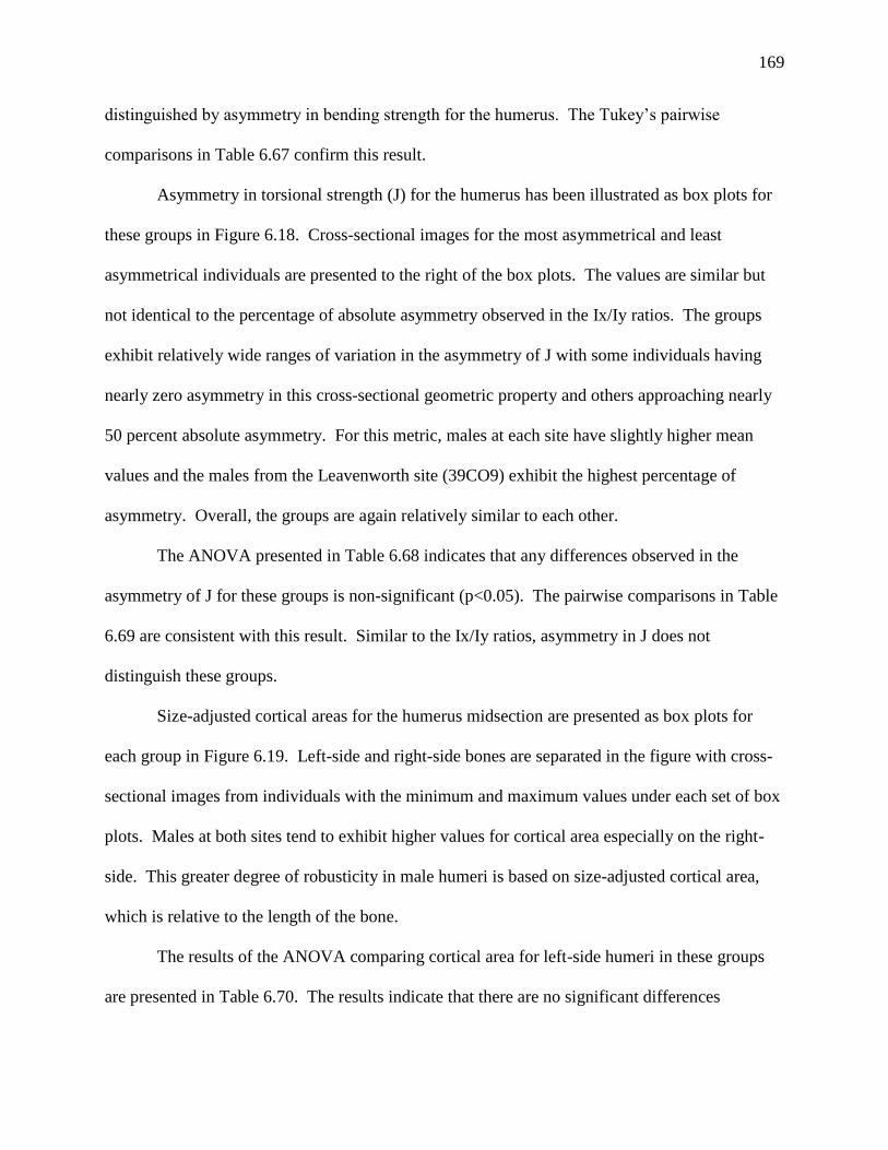
169

distinguished by asymmetry in bending strength for the humerus. The Tukey’s pairwise

comparisons in Table 6.67 confirm this result.

Asymmetry in torsional strength (J) for the humerus has been illustrated as box plots for

these groups in Figure 6.18. Cross-sectional images for the most asymmetrical and least

asymmetrical individuals are presented to the right of the box plots. The values are similar but

not identical to the percentage of absolute asymmetry observed in the Ix/Iy ratios. The groups

exhibit relatively wide ranges of variation in the asymmetry of J with some individuals having

nearly zero asymmetry in this cross-sectional geometric property and others approaching nearly

50 percent absolute asymmetry. For this metric, males at each site have slightly higher mean

values and the males from the Leavenworth site (39CO9) exhibit the highest percentage of

asymmetry. Overall, the groups are again relatively similar to each other.

The ANOVA presented in Table 6.68 indicates that any differences observed in the

asymmetry of J for these groups is non-significant (p<0.05). The pairwise comparisons in Table

6.69 are consistent with this result. Similar to the Ix/Iy ratios, asymmetry in J does not

distinguish these groups.

Size-adjusted cortical areas for the humerus midsection are presented as box plots for

each group in Figure 6.19. Left-side and right-side bones are separated in the figure with cross-

sectional images from individuals with the minimum and maximum values under each set of box

plots. Males at both sites tend to exhibit higher values for cortical area especially on the right-

side. This greater degree of robusticity in male humeri is based on size-adjusted cortical area,

which is relative to the length of the bone.

The results of the ANOVA comparing cortical area for left-side humeri in these groups

are presented in Table 6.70. The results indicate that there are no significant differences

170

Figure 6.19. Box plots of size adjusted cortical area for left and right humerus mid cross-sections. Images

for maximum and minimum values are presented below the box plots. The overextended medullary

cavities in the minimum cross-sectional images are not believed to have impacted these values.

171

Table 6.70. ANOVA results for left humerus mid size adjusted cortical area.

Test for equal means for left humerus mid cortical area

Sum of sqrs df Mean square F p (same)

Between groups: 3.91E-12 3 1.30E-12 1.751 0.1692

Within groups: 3.57E-11 48 7.44E-13

Total: 3.96E-11 51

Table 6.71. Tukey’s pairwise for left humerus mid size adjusted cortical area. (p-values in upper right). 39CO9F 39CO9M 39WW2F 39WW2M

39CO9F

0.9304 0.9651 0.4196

39CO9M 0.854

0.7062 0.1528

39WW2F 0.6665 1.521

0.7074

39WW2M 2.184 3.038 1.518

Table 6.72. ANOVA results for right humerus mid size adjusted cortical area.

Test for equal means for right humerus mid cortical area

Sum of sqrs df Mean square F p (same)

Between groups: 1.67E-11 3 5.58E-12 6.307 0.001154

Within groups: 3.98E-11 45 8.84E-13

Total: 5.65E-11 48

Table 6.73. Tukey’s pairwise for right humerus mid size adjusted cortical area (p-values in upper right). 39CO9F 39CO9M 39WW2F 39WW2M

39CO9F

0.02014* 0.9938 0.04955*

39CO9M 4.293

0.03875* 0.9834

39WW2F 0.3686 3.925

0.08938

39WW2M 3.779 0.514 3.411

172

(p<0.05) between the groups despite a trend towards more robust humeri among the males from

the Larson site (39WW2). The Tukey’s pairwise results in Table 6.71 are consistent with the

results of the ANOVA. There is a significant difference, however, between these groups for

right-side humeri according to the results of the ANOVA in Table 6.72. The Tukey’s pairwise

comparisons in Table 6.73 indicate that the most significant differences exist between males and

females from these sites with males exhibiting significantly greater amounts of cortical bone

relative to limb length.

Percentage of absolute asymmetry in cortical area for the humerus is illustrated as a box

plot in Figure 6.20. Images representing the left and right-side humeri for the most asymmetrical

and least asymmetrical individuals are presented to the right of the box plots. The individuals in

the sample exhibit a wide range of asymmetry for cortical area in the humerus with some

individuals exhibiting near zero and others exhibiting over 50 percent asymmetry.

The results of the ANOVA in Table 6.74 indicate that asymmetry in cortical area in the

humerus is significantly different (p<0.05) between these groups. The Tukey’s pairwise

comparisons in Table 6.75 indicate that the most significant difference exists between males and

females from the Leavenworth site (39CO9) with males exhibiting a greater degree of

asymmetry in robusticity between right and left-side humeri.

Comparison of Radius Cross-sections

Values for second moment of area ratios for the radius midsection are presented as box

plots in Figure 6.21. Right-side and left-side bones are presented separately in the figure with

cross-sectional images representing minimum and maximum values below each set of box plots.

All individuals in the analysis have Ix/Iy ratios below 1 indicating that they have the greatest

173

Figure 6.20. Box plots of humerus mid cortical area for percentage of absolute asymmetry by group. The

images to the right of the box plots are left and right subtrochanteric cross-sections for maximum (above)

and minimum (below) values. The overextended medullary cavities in these images are not believed to

have impacted these values.

Table 6.74. ANOVA results for humerus mid cortical area percent absolute asymmetry.

Test for equal means for humerus mid cortical area % absolute asymmetry

Sum of sqrs df Mean square F p (same)

Between groups: 1023.33 3 341.109 2.807 0.04974

Within groups: 5711.69 47 121.525

Total: 6735.02 50

Table 6.75. Tukey’s pairwise for humerus mid cortical area percent absolute asymmetry. (p-values in

upper right). 39CO9F 39CO9M 39WW2F 39WW2M

39CO9F

0.02232* 0.387 0.9159

39CO9M 4.228

0.5137 0.1031

39WW2F 2.267 1.962

0.7753

39WW2M 0.916 3.312 1.351

174

Figure 6.21. Box plots of Ix/Iy ratios for left and right radii mid cross-sections. Images for maximum and

minimum values are presented below the box plots. The overextended medullary cavity in the right-side

minimum cross-sectional image is not believed to have impacted these values.

175

Table 6.76. ANOVA results for left radius mid Ix/Iy ratio.

Test for equal means for left radius mid Ix/Iy ratio

Sum of sqrs df Mean square F p (same)

Between groups: 0.043446 3 0.014482 0.9573 0.4211

Within groups: 0.680768 45 0.015128

Total: 0.724215 48

Table 6.77. Tukey’s pairwise for left radius mid Ix/Iy ratio. (p-values in upper right). 39CO9F 39CO9M 39WW2F 39WW2M

39CO9F

0.8292 0.6029 0.5388

39CO9M 1.205

0.9794 0.96

39WW2F 1.759 0.5539

0.9997

39WW2M 1.904 0.6994 0.1455

Table 6.78. ANOVA results for right radius mid Ix/Iy ratio.

Test for equal means for right radius mid Ix/Iy ratio

Sum of sqrs df Mean square F p (same)

Between groups: 0.101043 3 0.033681 3.397 0.02552

Within groups: 0.456052 46 0.009914

Total: 0.557095 49

Table 6.79. Tukey’s pairwise for right radius mid Ix/Iy ratio. (p-values in upper right). 39CO9F 39CO9M 39WW2F 39WW2M

39CO9F

0.856 0.7619 0.478

39CO9M 1.126

0.2982 0.9151

39WW2F 1.385 2.511

0.08648

39WW2M 2.045 0.9193 3.43

176

resistance to bending stresses in the mediolateral dimension. Males tend to have average Ix/Iy

ratios that are higher than their female counterparts, although all of the groups appear relatively

similar.

The results of the ANOVA comparing Ix/Iy ratios at the left radius midsection in these

groups are presented in Table 6.76. They indicate that the observed differences in left radii are

not significant (p<0.05). The Tukey’s pairwise comparisons in Table 6.77 are consistent with

the results of the ANOVA. The results of the ANOVA comparing the Ix/Iy ratios for right-side

radii are presented in Table 6.78, indicating no significant differences. The pairwise

comparisons in Table 6.79 are consistent with the ANOVA.

Absolute asymmetry in the second moment of area ratios for the radius is presented as

box plots in Figure 6.22. There is a wide range of variation in asymmetry in the samples with

some individuals exhibiting almost no asymmetry and others exhibiting relatively high amounts

of asymmetry. Males from the Leavenworth site exhibit the highest degree of asymmetry in the

Ix/Iy ratio at the radius midsection with some individuals exceeding 60 percent absolute

asymmetry.

Despite the relatively wide range of variation for absolute asymmetry in these samples,

the variable does not distinguish these groups. The results of the ANOVA presented in Table

6.80 indicate that the groups do not differ significantly (p<0.05). The Tukey’s pairwise

comparisons in Table 6.81 are consistent with the results of the ANOVA indicating that none of

the groups differ significantly.

Percentage of absolute asymmetry in the polar second moment of area (J) at the

midsection of the radius is presented in the box plots in Figure 6.23. Cross-sectional images

representing left-side and right-side bones from the most asymmetrical and least asymmetrical

177

Figure 6.22. Box plots of radius mid Ix/Iy ratio values for percentage of absolute asymmetry by group.

The images to the right of the box plots are left and right subtrochanteric cross-sections for maximum

(above) and minimum (below) values.

Table 6.80. ANOVA results for radius mid Ix/Iy ratio percent absolute asymmetry.

Test for equal means for radius mid Ix/Iy ratio % absolute asymmetry

Sum of sqrs df Mean square F p (same)

Between groups: 775.249 3 258.416 1.652 0.1926

Within groups: 6255.58 40 156.39

Total: 7030.83 43

Table 6.81. Tukey’s pairwise for radius mid Ix/Iy ratio percent absolute asymmetry. (p-values in upper

right). 39CO9F 39CO9M 39WW2F 39WW2M

39CO9F

0.07126 0.6537 0.8772

39CO9M 3.571

0.5296 0.299

39WW2F 1.644 1.927

0.9757

39WW2M 1.057 2.514 0.5867

178

Figure 6.23. Box plots of radius mid J for percentage of absolute asymmetry by group. The images to the

right of the box plots are left and right subtrochanteric cross-sections for maximum (above) and minimum

(below) values.

Table 6.82. ANOVA results for radius mid J percent absolute asymmetry.

Test for equal means for radius mid J % absolute asymmetry

Sum of sqrs df Mean square F p (same)

Between groups: 128.967 3 42.9891 0.3491 0.79

Within groups: 4925.87 40 123.147

Total: 5054.84 43

Table 6.83. Tukey’s pairwise for radius mid J percent absolute asymmetry. (p-value in upper right). 39CO9F 39CO9M 39WW2F 39WW2M

39CO9F

0.9146 0.8229 0.9474

39CO9M 0.9207

0.9966 0.9996

39WW2F 1.223 0.3024

0.9886

39WW2M 0.771 0.1497 0.452

179

individuals in the sample are presented to the right of the box plots in the figure to provide some

context for the numbers. Barring a few exceptions, the groups exhibit relatively low values for

asymmetry in resistance to torsional forces. Most individuals fall below 30 percent asymmetry

for J.

The ANOVA in Table 6.82 indicates the groups do not differ significantly (p<0.05). The

pairwise comparisons in Table 6.83 are consistent with the ANOVA indicating that the groups

are relatively similar in the amount of asymmetry they exhibit in the polar second moment of

area at the radius midsection.

Size adjusted cortical area for the radius midsection is presented in the box plots in

Figure 6.24. Left and right-side bones are separated in the figure with cross-sectional images

representing the minimum and maximum values below each set of box plots. For left-side

cortical area in the radius, females from the Leavenworth site (39CO9) have the highest values in

the sample. The groups appear more similar for right-side elements. As a general trend, females

have average cortical areas that are higher than their male counterparts at each site.

The result of the ANOVA comparing left-side radius cortical areas indicates that these

groups do differ significantly (p<0.05) (Table 6.84). The Tukey’s pairwise comparisons in Table

6.85 indicate that the most significant difference exists between males and females at the

Leavenworth site. Females from Leavenworth exhibit significantly higher values for size-

adjusted cortical area indicating they experience relatively greater resistance to compressive

force in the left radius. Right-side radii do not exhibit difference between these groups despite

the trend towards higher cortical area values among females at each site. The ANOVA in Table

6.86 and the pairwise comparisons in Table 6.87 indicate that no significant differences exist for

right side radii.

180

Figure 6.24. Box plots of size adjusted cortical area for left and right radii mid cross-sections. Images for

maximum and minimum values are presented below the box plots. The overextended medullary cavity in

the right-side cross-section is not believed to have impacted these values.

181

Table 6.84. ANOVA results for left radius mid size adjusted cortical area.

Test for equal means for left radius mid size adjusted cortical area

Sum of sqrs df Mean square F p (same)

Between groups: 5.45E-12 3 1.82E-12 3.076 0.03866

Within groups: 2.31E-11 39 5.91E-13

Total: 2.85E-11 42

Table 6.85.Tukey’s pairwise for left radius mid size adjusted cortical area. (p-value in upper right). 39CO9F 39CO9M 39WW2F 39WW2M

39CO9F

0.03427* 0.1606 0.09415

39CO9M 4.022

0.8924 0.9702

39WW2F 3.017 1.005

0.9934

39WW2M 3.392 0.6297 0.3751

Table 6.86. ANOVA results for right radius mid size adjusted cortical area.

Test for equal means for right radius mid size adjusted cortical area

Sum of sqrs df Mean square F p (same)

Between groups: 1.07E-12 3 3.58E-13 0.4702 0.7046

Within groups: 3.20E-11 42 7.61E-13

Total: 3.30E-11 45

Table 6.87. Tukey’s pairwise for right radius mid size adjusted cortical area. (p-value in upper right). 39CO9F 39CO9M 39WW2F 39WW2M

39CO9F

0.5712 0.9432 0.9962

39CO9M 1.832

0.8827 0.7074

39WW2F 0.7927 1.039

0.9865

39WW2M 0.3134 1.518 0.4793

182

Figure 6.25. Box plots of radius mid cortical area for percentage of absolute asymmetry by group. The

images to the right of the box plots are left and right subtrochanteric cross-sections for maximum (above)

and minimum (below) values.

Table 6.88. ANOVA results for radius mid cortical area percent absolute asymmetry.

Test for equal means for radius mid cortical area % absolute asymmetry

Sum of sqrs df Mean square F p (same)

Between groups: 252.989 3 84.3298 1.192 0.3249

Within groups: 2828.7 40 70.7175

Total: 3081.69 43

Table 6.89. Tukey’s pairwise for radius mid cortical area percent absolute asymmetry. (p-values in upper

right) 39CO9F 39CO9M 39WW2F 39WW2M

39CO9F

0.2017 0.9476 0.649

39CO9M 2.842

0.4676 0.8354

39WW2F 0.7696 2.072

0.9232

39WW2M 1.655 1.187 0.885

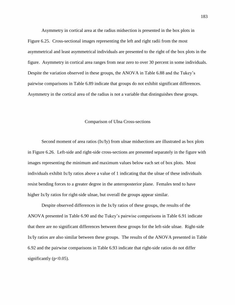
183

Asymmetry in cortical area at the radius midsection is presented in the box plots in

Figure 6.25. Cross-sectional images representing the left and right radii from the most

asymmetrical and least asymmetrical individuals are presented to the right of the box plots in the

figure. Asymmetry in cortical area ranges from near zero to over 30 percent in some individuals.

Despite the variation observed in these groups, the ANOVA in Table 6.88 and the Tukey’s

pairwise comparisons in Table 6.89 indicate that groups do not exhibit significant differences.

Asymmetry in the cortical area of the radius is not a variable that distinguishes these groups.

Comparison of Ulna Cross-sections

Second moment of area ratios (Ix/Iy) from ulnae midsections are illustrated as box plots

in Figure 6.26. Left-side and right-side cross-sections are presented separately in the figure with

images representing the minimum and maximum values below each set of box plots. Most

individuals exhibit Ix/Iy ratios above a value of 1 indicating that the ulnae of these individuals

resist bending forces to a greater degree in the anteroposterior plane. Females tend to have

higher Ix/Iy ratios for right-side ulnae, but overall the groups appear similar.

Despite observed differences in the Ix/Iy ratios of these groups, the results of the

ANOVA presented in Table 6.90 and the Tukey’s pairwise comparisons in Table 6.91 indicate

that there are no significant differences between these groups for the left-side ulnae. Right-side

Ix/Iy ratios are also similar between these groups. The results of the ANOVA presented in Table

6.92 and the pairwise comparisons in Table 6.93 indicate that right-side ratios do not differ

significantly (p<0.05).

184

Figure 6.26. Box plots of Ix/Iy ratios for left and right ulna mid cross-sections. Images for maximum and

minimum values are presented below the box plots.

185

Table 6.90. ANOVA results for left ulna mid Ix/Iy ratio.

Test for equal means for left ulna mid Ix/Iy ratio

Sum of sqrs df Mean square F p (same)

Between groups: 0.048504 3 0.016168 0.1732 0.9139

Within groups: 3.92017 42 0.093338

Total: 3.96868 45

Table 6.91. Tukey’s pairwise for left ulna mid Ix/Iy ratio. (p-values in the upper right) 39CO9F 39CO9M 39WW2F 39WW2M

39CO9F

1 0.9837 0.9985

39CO9M 0.05568

0.9884 0.997

39WW2F 0.5108 0.4552

0.9525

39WW2M 0.2323 0.288 0.7432

Table 6.92. ANOVA results for right ulna mid Ix/Iy ratio.

Test for equal means for right ulna mid Ix/Iy ratio

Sum of sqrs df Mean square F p (same)

Between groups: 0.247126 3 0.082375 1.125 0.3484

Within groups: 3.51514 48 0.073232

Total: 3.76226 51

Table 6.93. Tukey’s pairwise for right ulna mid Ix/Iy ratio. (p-values in the upper right). 39CO9F 39CO9M 39WW2F 39WW2M

39CO9F

0.4668 0.9618 0.9823

39CO9M 2.071

0.2212 0.6962

39WW2F 0.6879 2.759

0.826

39WW2M 0.5263 1.544 1.214

186

Figure 6.27. Box plots of ulna mid Ix/Iy ratio values for percentage of absolute asymmetry by group. The

images to the right of the box plots are left and right subtrochanteric cross-sections for maximum (above)

and minimum (below) values.

Table 6.94. ANOVA results for ulna mid Ix/Iy ratio percent absolute asymmetry.

Test for equal means for ulna mid Ix/Iy ratio % absolute asymmetry

Sum of sqrs df Mean square F p (same)

Between groups: 1105.32 3 368.441 1.621 0.1996

Within groups: 9089.51 40 227.238

Total: 10194.8 43

Table 6.95. Tukey’s pairwise for ulna mid Ix/Iy ratio percent absolute asymmetry. (p-values in the upper

right). 39CO9F 39CO9M 39WW2F 39WW2M

39CO9F

0.9054 0.5143 0.2963

39CO9M 0.9569

0.8922 0.6877

39WW2F 1.963 1.006

0.9788

39WW2M 2.522 1.565 0.5594

187

Absolute asymmetry in Ix/Iy ratios for the ulna midsection are presented as box plots in

Figure 6.27. Right and left-side cross-sectional images for the most and least asymmetrical

individuals are presented on the right side of the figure. The box plots indicate that there is a

wide range in the values, with some individuals exhibiting nearly zero asymmetry in Ix/Iy ratios

and others exhibiting nearly 90 percent asymmetry between right and left-side ulnae. Females

from the Leavenworth site (39CO9) exhibit the greatest range of variation.

Despite the variation observed in the sample, the ANOVA presented in Table 6.94

indicates the differences between these groups are not significant at the p<0.05 level. The

Tukey’s pairwise comparisons in Table 6.95 are consistent with the ANOVA results.

Asymmetry in Ix/Iy ratios at the ulna midsection is not a variable that distinguishes the groups

used in this analysis.

Absolute asymmetry in the second moment of area (J) at the ulna midsection is presented

as box plots in Figure 6.28, with cross-sectional images representing maximum and minimum

values presented to the right of the box plots in the figure. The values range from near zero to

over 50 percent asymmetry. The groups all appear relatively similar in their average asymmetry

values for J.

The ANOVA in Table 6.96 confirms what is visually apparent in the box plots. The

results indicate that any observed differences in the mean value are not significant at the p<0.05

level. The Tukey’s pairwise comparisons in Table 6.97 are consistent with the results of the

ANOVA and indicate that no differences exist between these groups.

Values for size-adjusted cortical area at the ulna midsection are illustrated as box plots in

Figure 6.29. Right and left-side bones are separated in the figure and cross-sectional images

representing the minimum and maximum values are presented below each set of box plots. For

188

cortical area in the ulna, females at each site exhibit a greater range of variation. Mean values

for each group, however, are relatively similar. The observation that these groups are relatively

similar is supported by the ANOVA results and Tukey’s comparisons presented in Tables 6.98 –

6.101, with no significant differences observed.

Finally, absolute asymmetry in cortical area at the ulna midsection is displayed as box

plots in Figure 6.30. These groups exhibit a range of variation from near zero to over 40 percent

asymmetry in cortical area. Females from each site, again, exhibit greater variation than do their

male counterparts. The results of the ANOVA comparing asymmetry in cortical area at the ulna

midsection indicate no significant differences exist between the groups (Table 6.102). The

pairwise comparisons in Table 6.103 support the results of the ANOVA.

189

Figure 6.28. Box plots of ulna mid J for percentage of absolute asymmetry by group. The images to the

right of the box plots are left and right subtrochanteric cross-sections for maximum (above) and minimum

(below) values. The overextended medullary cavity in the minimum cross-sections is not believed to

have impacted these values.

Table 6.96. ANOVA results for ulna mid J percent absolute asymmetry.

Test for equal means for ulna mid J % absolute asymmetry

Sum of sqrs df Mean square F p (same)

Between groups: 588.604 3 196.201 0.9805 0.4116

Within groups: 8003.83 40 200.096

Total: 8592.44 43

Table 6.97. Tukey’s pairwise for ulna mid J percent absolute asymmetry. (p-values in upper right). 39CO9F 39CO9M 39WW2F 39WW2M

39CO9F

0.8438 0.5963 0.9862

39CO9M 1.162

0.9725 0.9631

39WW2F 1.775 0.6126

0.7978

39WW2M 0.4831 0.6794 1.292

190

Figure 6.29. Box plots of size adjusted cortical area for left and right ulna mid cross-sections. Images for

maximum and minimum values are presented below the box plots.

191

Table 6.98. ANOVA results for left ulna mid size adjusted cortical area.

Test for equal means for left ulna mid size adjusted cortical area

Sum of sqrs df Mean square F p (same)

Between groups: 2.33E-12 3 7.78E-13 0.9471 0.4295

Within groups: 2.63E-11 32 8.21E-13

Total: 2.86E-11 35

Table 6.99. Tukey’s pairwise for left ulna mid size adjusted cortical area. (p-values in upper right). 39CO9F 39CO9M 39WW2F 39WW2M

39CO9F

0.3801 0.5712 0.6146

39CO9M 2.297

0.9879 0.9785

39WW2F 1.835 0.4614

0.9999

39WW2M 1.736 0.561 0.09961

Table 6.100. ANOVA results for right ulna mid size adjusted cortical area.

Test for equal means for right ulna mid size adjusted cortical area

Sum of sqrs df Mean square F p (same)

Between groups: 5.14E-13 3 1.71E-13 0.2497 0.8611

Within groups: 3.02E-11 44 6.87E-13

Total: 3.07E-11 47

Table 6.101. Tukey’s pairwise for right ulna mid size adjusted cortical area. (p-values in upper right). 39CO9F 39CO9M 39WW2F 39WW2M

39CO9F

0.9998 0.9424 1

39CO9M 0.1291

0.9133 0.9998

39WW2F 0.7971 0.9263

0.9405

39WW2M 0.008994 0.1202 0.8061

192

Figure 6.30. Box plots of ulna mid cortical area for percentage of absolute asymmetry by group. The

images to the right of the box plots are left and right subtrochanteric cross-sections for maximum (above)

and minimum (below) values.

Table 6.102. ANOVA results for ulna mid cortical area percent absolute asymmetry.

Test for equal means for ulna mid cortical area % absolute asymmetry

Sum of sqrs df Mean square F p (same)

Between groups: 95.4675 3 31.8225 0.3056 0.8211

Within groups: 4164.63 40 104.116

Total: 4260.1 43

Table 6.103. Tukey’s pairwise for ulna mid cortical area percent absolute asymmetry. (p-values in the

upper right). 39CO9F 39CO9M 39WW2F 39WW2M

39CO9F

0.789 0.9114 0.9767

39CO9M 1.315

0.9931 0.9536

39WW2F 0.9337 0.3817

0.9944

39WW2M 0.5782 0.7372 0.3555

193

CHAPTER 7

DISCUSSION AND CONCLUSIONS

My goal with this dissertation has been to explore the impact that the expansion of

Europeans and Americans had on the lives of the Plains Village Horticulturalists through an

examination of human skeletons from cemeteries associated with Sahnish villages. The analysis

relies heavily on the interpretation of limb bone cross-sectional shape to understand how activity

patterns may have changed from the beginning of the Post-Contact era to just prior to the

complete abandonment of the Plains Village lifeway. The study builds upon previous research

examining limb bone cross-sectional geometry (CSG) to understand activity in past populations.

In these studies, the arrangement of cortical bone in a cross-section is discussed in terms of bone

strength and interpreted as reflecting how the bone developed to resist the biomechanical forces

associated with habitual activities. I have added an additional layer to the typical CSG study by

including a comparison of biological distance to understand the underlying relationships between

individuals in the sample so that I may be able to provide a more robust interpretation of the

findings. To that end, I have posed a number of questions that were formalized as testable

hypotheses in Chapter 5 all of which revolve around broader themes. Were mobility patterns

significantly altered by the arrival of new groups on the Great Plains? Did the work loads of

women increase with new trading partners and their entrance into the Euroamerican fur markets?

Did hunting activities change substantially after the adoption of the gun? Perhaps most

194

importantly, can the skeleton provide us with clues to those changing activities? This last

question is of paramount importance since variation may have been introduced through gene

flow during the Post-Contact period. In the following sections, I will discuss how the results

from Chapter 6 can be used to address these questions.

Discussion of the Specific Hypotheses

The specific hypotheses outlined in Chapter 5 provide a starting point for understanding

the changes that occurred during the Post-Contact period. They address how biological variation

may have changed between the occupation of the Larson site (39WW2) and the Leavenworth site

(39CO9), with the specific goal of understanding how activity patterns were altered in response

to a suite of cultural changes. The hypotheses were developed to rigorously explore the dataset

with the hope of identifying whether the sources of variation were environmental or genetic. The

first set of hypotheses (referred to here as Hypotheses 1a and 1b) focused on distinguishing

whether shifting patterns of variation were the result of new alleles in the gene pool or if cultural

changes could explain the differences. They were designed to test whether related individuals,

that is individuals who share biological kinship, have similarities in the shape of their limbs. If

that was found to be the case, then it calls into question the interpretation of activity from the

skeleton. If biological kin have limb bones that look the same, then differences identified in

these samples may be attributed to new genes that were introduced during the Post-Contact

period rather than the adoption of new activity patterns. If, however, the limb bones of

biological kin vary randomly, then it lends support to the idea we may detect the repetitive

activities of individuals through examining their limbs. The second set of hypotheses (referred

to here as Hypotheses 2a – 2h) address those activities. The series of testable hypotheses related

195

to cross-sectional geometry were designed to explore some of the possible activity changes that

occurred during the Post-Contact period. In this section, I will review how the results reported in

Chapter 6 inform each hypothesis.

Based upon the Mantel results comparing the intergroup pairwise distances, I could not

fully reject the null hypothesis for Hypothesis 1a, which states that between group biological

distance will not correlate with distance based on limb bone geometry. Both the raw

measurements and size-transformed datasets provide similar results, indicating limb bone

variables at some specific loci and odontometric data from the same individuals created

Mahalanobis distance matrices that do not exhibit similar patterns (see Tables 6-15 thru 6-18 in

the previous chapter). The alternative hypothesis that group distance matrices will exhibit

correlations is supported in some cases. Distances created from the odontometric data exhibited

moderate to high correlations with distances created from loci on the right-side femur, humerus,

and radius (size adjusted only) and the left-side femur midsection. Overall, the pattern varies

depending on which limb bone locus is included in the analysis. The femur midshaft is the most

consistently correlated, with both right and left sides exhibiting significant correlations with the

distances based on odontometric data. In this analysis, support for the alternative hypothesis

indicates that caution should be taken when interpreting differences between the limb bones of

these groups. The results do not explicitly indicate that the limb bone data at these loci reflect

genetic variation, but alternative explanations for the pattern must be addressed with caution. In

the next section, I will provide a nuanced interpretation of this pattern.

Likewise, there are mixed results for Hypothesis 1b: within groups biological distance

will correlate with distance based on limb bone geometry. The intragroup results also indicate

that, at certain loci, correlations exist between distance scores created from odontometrics

196

(biological distance) and distances created from limb bone variables. The presence of some

significant correlations in Table 6-19 between pairwise distance matrices created from the limb

bone data and those created from the odontometric dataset indicates that the null Hypothesis 1b,

which states that biological distance between individuals based on odontometric data will not

correlate with distances based on limb bone cross-sectional geometry, cannot be fully rejected.

Even though these were weak correlations, their significance indicates that individuals within the

sample occupy multivariate space with nonrandom similarity whether the dataset be

odontometric data or limb bone data from certain cross-sectional loci. Specifically, individuals

with similarities in the odontometric data also exhibit some similarity in cross-sectional limb

morphology from the left humerus, the right radius (size-adjusted only), and the right ulna (size-

adjusted only). In the forearm, the correlation for the left ulna is approaching the level of

significance with a p-value of 0.09. The pattern is different than what was identified in the group

distances, with considerably fewer loci exhibiting significant correlations. While the null

hypothesis cannot be rejected for the dataset as a whole, the results seem to indicate that, for

most bones, cross-sectional variables are not very similar among biological kin.

Hypothesis 1 (including both 1a and 1b) was developed to test the long-held assumption

among some bioarchaeologists that limb bone cross-sectional geometry is not inherited and

instead reflects biomechanical loading patterns that individuals experience during their lifetimes.

This assumption has been criticized by some authors, who have suggested much of the shape of

the limb is set early during development before the habitual activities that might reshape the limb

would occur and therefore may be telling us more about genetic variation within a population

than variation in activity (e.g., Lovejoy et al., 2003; Pearson and Lieberman, 2004). The results

of this analysis are mixed, but they favor the idea that limb bone cross-sections do not reflect

197

genetic relationships between individuals. In the cases where biological kin (blood relatives)

seem to share limb bone cross-sectional shape, an activity-based explanation may be more

appropriate. In the intergroup analyses, the femur midshaft, for example, exhibits similarity

among groups that appear to be the most similar based on their dentition. This could suggest that

the midshaft of the femur retains genetic markers that are shared between biological kin groups,

but considering the femur is under significant biomechanical stress and bones under less

biomechanical stress exhibit no such correlation, the genetic explanation appears less likely. A

more probable explanation appears to be that kin groups were engaging in similar activities,

creating a pattern that may mirror genetic relationships in some cases. This somewhat

paradoxical result may relate to Sahnish residency patterns and is discussed in greater detail in

the following section. Ultimately, the results I have presented here fail to reject the null

hypothesis that limb bone cross-sectional geometry is not inherited, lending support to their

continued use in this study and others that seek to understand variation in activity patterns.

The cross-sectional geometric properties presented in Chapter 6 provide ample results to

discuss the hypotheses outlined in Chapter 5 under Hypothesis 2 – Effects of sex-specific activity

on cross-sectional geometry. Those hypotheses address a number of questions related to sexual

dimorphism resulting from sex-specific activities that have been inferred from historical

accounts and the archaeological record. They also address questions related to temporal trends

among these groups, specifically the hypothesized changes in activity patterns resulting from the

disruption of traditional lifeways experienced by individuals living at the Leavenworth site

(39CO9). Hypotheses 2a through 2c relate directly to patterns that may be apparent based a

sexual division of labor, much of which is based upon information gleaned from the

ethnohistoric record (e.g., Brackenridge et al., 1904; Moulton, 1987). The remaining hypotheses,

198

2d through 2h, relate to changes that may have occurred between the two sites. These relate to

specific activities that may have changed as the Sahnish took on a more direct role in the

Euroamerican trade networks and as pressure from outside groups reduced the size of their

territory (Holder, 1970; Rogers, 1990; Krause, 2016; Murray and Swenson, 2016).

The null hypothesis for Hypothesis 2a, which states that males and females will not

exhibit significant differences in the asymmetry of CSG variables in the upper limb, cannot be

fully rejected. The alternative hypothesis postulates that males will exhibit significantly more

asymmetry in the upper limb, likely due to their use of the bow and arrow. Males do exhibit

significantly higher values for the percentage of absolute asymmetry in cortical area in the

humerus at 39CO9 (Leavenworth) (see Figure 6.20 and Table 6.75), but no other differences in

asymmetry for any of the bones of the upper limb reached the level of statistical significance.

The trend towards asymmetry in the strength of the upper limbs of males, if linked to the use of

the bow, should be evident in males from both sites since all males would have engaged in the

activity. There is a trend towards greater asymmetry in males for J (torsional strength), though

differences between males and females fail to reach the critical value for significance (see Figure

6.18).

It is possible that this trend towards more asymmetry in torsional strength in male humeri

may be related to the use of the bow, but the activity is not intense enough or habitual enough to

create statistically significant differences between the sexes. The accounts by Brackenridge and

Clark indicate that, at least during the historic period, the Sahnish men led rather leisurely lives

when not engaged in hunting activities, which may indicate that bow use was somewhat sporadic

and not habitual enough to lead to significant differences (Brackenridge et al., 1904; Moulton,

1987). The greater cortical strength in male humeri, however, suggests that males were engaging

199

in activities that required more compressive strength than females in their upper limbs. Those

activities apparently did not involve a great deal of torsion on the bone, like would be expected

with the use of the bow. It remains unclear exactly what those activities may have been, but

general robusticity in the arms may indicate that these males were carrying heavier loads than

their female counterparts.

The null hypothesis for Hypothesis 2b, which states that males and females will not

exhibit significant differences in the asymmetry of CSG variables in the lower limb, cannot be

fully rejected. In the tibia, asymmetry in cross-sectional variables was not significantly different

between males and females. In the femur, however, there is support for the alternative

hypothesis that males and females differ in asymmetry of certain cross-sectional variables.

Females from the Leavenworth site (39CO9) exhibit significantly more asymmetry than do their

male counterparts in bending strength (Ix/Iy ratio) at the subtrochanteric region (see Figure 6.2).

At the midsection of the femur, females from Leavenworth have significantly higher values for

torsional strength (J) and compressive strength (cortical area) (see Figures 6.8 & 6.10). This

provides some support for the alternative hypothesis that female stance during horticultural

activities may result in lower limb asymmetry. However, the trend is only noted at Leavenworth,

and horticulture is a subsistence pattern known to exist at both sites. Therefore, horticultural

activities alone do not explain the trend. There may be additional cultural practices that were

adopted at Leavenworth that led to the development of the lower limb asymmetry at that site.

This is explored further in Hypothesis 2g.

The null hypothesis for Hypothesis 2c, which states that males and females will not

exhibit significant differences in bending strength for the bones of the lower limb, cannot be

rejected on the basis of the data presented here. The alternative hypothesis that males will have

200

greater resistance to bending stress in the anteroposterior plane due to more running and long

distance travel finds only minimal support as some values trend in that direction, though they do

not reach the level of significance. Males at the Larson site (39WW2) do exhibit higher values

for the second moment of area ratios in the ANOVA indicating they have tibiae that are more

resistant to anteroposterior bending stresses, but the differences are not significant at the 0.05

level when compared to females from the same site (see Tables 6.48 thru 6.51). The right-side

values for the tibia, however, are approaching significance. Although the differences do not

reach the critical value for statistical significance, the mean values for Ix/Iy ratios are

consistently higher for males at the midshaft of the tibia and the femur for both groups indicating

a trend toward greater anteroposterior bending resistance among males. A larger sample might

confirm that this difference is real and not due to chance alone.

In general, the results from the lower limb suggest that males may have only been

marginally more mobile than their female counterparts. This may relate to the manner in which

hunting was performed. Historic accounts indicate that the entire village was abandoned during

the summer and winter months for hunting expeditions, which suggests men and women were

both leaving for this long-range travel (Owsley et al., 1977). Perhaps the slight differences in

bending strength that are noted above relate more to male mobility within the village than it does

their long-range hunting strategies. Brackenridge notes that males were engaged in a fair amount

of sport during his visit in 1811, which may provide evidence that males were doing more

running during the day than their female counterparts (Brackenridge et al, 1904:120). Perhaps

these sporting activities and more opportunistic hunting around the village led males to develop

slightly greater bending strength in their lower limbs, but these activities were not frequent or

intense enough to create significant differences between males and females.

201

The null hypothesis for Hypothesis 2d, which states that bending strength will not change

in males over time, cannot be fully rejected since not all second moment of area ratios (Ix/Iy

ratios) in the lower limb differ significantly for males. In the tibia, however, there is support for

the alternative hypothesis that male bending strength will be reduced at the Leavenworth site

(39CO9). Second moment of area ratios for the right tibia are lower for males at the

Leavenworth site indicating a significant reduction in their resistance to anteroposterior bending

(see Figure 6.11 and Table 6.51). The reduction in the Ix/Iy ratio is approaching the level of

significance for the left tibia as well. The null hypothesis cannot be rejected for the femur,

however. Second moment of area ratios for the femur remain relatively similar for males in both

groups.

The null hypothesis for Hypothesis 2e, which states that males will not exhibit significant

differences over time in the ability of the lower limb to resist compressive forces, cannot be

rejected on the basis of the data presented in Chapter 6. Average size-adjusted cortical area is

lower in the femur and tibia among the males at the Leavenworth site (39CO9), though the

difference is not statistically significant when compared to their male counterparts from the

Larson site. This trend towards more gracile limbs suggests some support for the alternative

hypothesis that a reduction in mobility at Leavenworth would lead to lower cortical area in

males. However, this is only an observed trend and none of the analyses reach the critical value

needed to reject the null hypothesis.

Hypotheses 2d and 2e both suggest that something occurred between the occupation of

the Larson site and Leavenworth that led to a reduction in lower limb strength variables among

the males. This may relate to the introduction of the horse in 1738, which was likely not a factor

in the mobility of males at the Larson site. We may be observing a shift away from long-range

202

hunting on foot. By utilizing the horse for transportation, much of the stress on the lower limb

would be alleviated during long-range travel, which would result in less bending and

compression on the lower limb. Alternatively, or perhaps in addition to the addition of the horse,

conflicts with outside groups may have limited the amount of travel males engaged in at

Leavenworth. These changes may be enough to result in the observed differences.

The null hypothesis for Hypothesis 2f, which states that males will not exhibit

significantly different CSG asymmetry in the humerus, radius, and ulna, cannot be rejected. The

alternative hypothesis that asymmetry in the upper limbs of males would have reduced over time

as the use of the bow became less necessary is not supported by the asymmetry data examined in

this study. The introduction of firearms in 1750 may not have completely supplanted the use of

the bow (Rogers, 1990). Brackenridge, for example, mentions both weapons being used in

warfare and hunting, which may indicate that the gun did not play such a significant role in these

villages that the use of the bow and arrow was not a regular occurrence for the males at

Leavenworth (Brackenridge et al, 1904:118).

The null hypothesis for Hypothesis 2g, which states that females will not exhibit

significant changes in the asymmetry of CSG values in the lower limb over time, cannot be fully

rejected on the basis of the data presented in Chapter 6. There were no significant differences

between females in the asymmetry of the tibia. When examining the femur, however, there is

some support for the alternative hypothesis that asymmetry would have increased among the

females at the Leavenworth site (39CO9) due to an intensification of horticulture. Females from

the Leavenworth site exhibit significantly higher percentages of absolute asymmetry in second

moment of area ratios (Ix/Iy) at the subtrochanteric region (Table 6.25), polar second moment of

area (J) at the midsection (Table 6.41), and cortical area at the midsection (Table 6.47). It should

203

be noted, however, that much of the asymmetry in anteroposterior bending strength (Ix/Iy ratio)

in the subtrochanteric region of the femur can be attributed to an extreme amount of torsion

among some females from the Leavenworth site (Figure 7.1). The torsion identified in this study

mirrors that observed by Wescott et al. (2014), who suggested it may be the result of a habitual

side-sitting posture adopted by the Sahnish women during the historic period. This

interpretation, however, is perhaps overly simplistic and suggests that side-sitting was adopted

from a young age. What may be more likely, is that young women were being conscripted for

work at a younger and younger age to meet the demands of the new trade networks, during

which time they are sitting or standing in postures that led to extreme torsion in the femur.

Finally, the null hypothesis for Hypothesis 2h, which states that compressive strength will

not change over time in the upper limb of females, cannot be rejected. There is no support for

the alternative hypothesis that females from the Leavenworth site (39CO9) will exhibit

significantly greater cortical area in the upper limb due to an intensification of processing

activities related to trade. There is a slight trend for females from the Leavenworth site to exhibit

an increase in the average values for cortical area in the left radius and left ulna (see Figures 6.24

and 6.29), but the difference between the sites is far from significant. This seems to suggest that

women at both villages engaged in similar types of activities, at least when using their upper

limbs.

General Discussion of Themes

The results of this analysis provide interesting patterns that are worth discussing beyond

the language of hypothesis testing. While the results discussed above provide a place to start the

conversation, there are other patterns that became apparent during my analysis of these sites that

204

Figure 7.1. Example of torsion in the femur of a Leavenworth female.

205

are worth exploring. There are also broader themes that are apparent in the data that cross-cut

the hypotheses reviewed above. These topics deserve further exploration.

The coefficients of variation reported in the summary statistics are relatively low for the

dentition, indicating that these populations exhibit limited variation in the morphology of their

teeth (see Tables 6.1 and 6.2). Surprisingly, females in these samples exhibit slightly greater

variation than males for many of the dental metrics, which is unexpected for matrilocal

populations. One would expect significantly more variation among the males if they are leaving

their natal group, but that is not the pattern in the samples collected for this analysis. The

differences between male and female dental variation appear minor, however, and may be a

result of the small sample sizes used in this analysis. It is unclear if the variation is

representative of these populations as a whole, but the pattern appears relatively similar at both

sites, suggesting that slightly higher dental variation among females spans the temporal gap

between the sites. It should be noted, however, that these are simply observed patterns in the

summary statistics. I did not explicitly test for significant difference in dental variation between

these groups.

The multivariate distance scores for these groups may provide a stronger measurement

than the coefficient of variation for understanding how residency patterns have influenced the

overall structure of the villages. Many of the distance scores indicate that between these sites

females are more similar to each other than are the males (see Tables 6-15 thru 6-18). This

suggests that even though within each village the female dentition exhibits slightly higher

variation, between the sites females remain more similar while the males diverge over time. This

seems to reflect the pattern of matrilocal residency noted historically among the Sahnish (Parks,

2001a). Interestingly, this is pattern holds true for both the dentition and the limb-bone data,

206

suggesting that either the limbs are following a similar pattern as the teeth (data I am using for a

genetic proxy) or that this sample is detecting a convergence between the genetic similarities and

similarities in activities. Since the tests of correlation between dental and limb-bone data

showed only very limited correlations, it would appear that the latter is the case – we are

detecting convergence of genetic ties between people and similar activity patterns.

The pattern observed in the distance scores plays out in the Mantel results of correlations

between distance matrices. Comparing the two sites, the correlations between distance matrices

appears to be driven by differences between sexes. For many of the loci, both dental and limb

bone variables created distance scores that exhibit a similar pattern, with the femur, humerus and

radius all creating distance scores that indicate, like the teeth, that between sites females are

more similar to each other than are the males (see Tables 6-15 thru 6-18). The correlation

coefficients for these tests were slightly higher when the raw, unscaled variables were used in the

analysis, suggesting inherent size differences between males and females may contribute to the

pattern. However, the pattern is consistent even when these variables were scaled to account for

differences in body size. This is likely due to genetic and behavioral convergence at the level of

sex, with a sexual division of labor driving the analysis. Post-marital matrilocal residency

patterns among the Sahnish would create a scenario where men in these populations were

genetically dissimilar while women were more similar. Genetic similarities between the females

at each site seem to be borne out in the Mahalanobis D scores for the odontometric data. Female

activities at each site may have been similar enough to mirror the genetic patterns that developed

through matrilocal residency, with closer distance scores between the females from each site

regardless of whether those distance scores were generated from the teeth or from the limbs.

Males at each site exhibit relatively more dissimilarity for many of the loci, which may indicate

207

that the cultural changes had a greater impact on the males. With reduced mobility and changes

to hunting technology, we may expect the males from each site to be relatively more different

than the females. This pattern may coincidentally mirror the genetic differences since males are

not staying with their natal groups. The inclusion of an outgroup in future analyses would help

to clarify this issue.

Intragroup biological distance scores exhibit a different pattern than the between group

analyses (see Table 6-19). Within the sample, most distance matrices created from limb bone

cross-sectional data did not correlate with distance matrices created from the dentition for the

same individuals, the exception being the left humerus and some bones of the forearm. How

might the differences between the intragroup and intergroup analyses be explained? Regardless

of the activities performed or the intensity of those activities, certain biomechanical patterns will

be maintained. Handedness, for example, will be a constant regardless of the activities

performed. This may explain why the left-side humerus exhibits a significant correlation in the

intragroup analysis but not in the between group analyses. Biological kin, regardless of the

activities they perform, are likely to favor their dominant side. Therefore, the non-dominant side

(most frequently the left) should reflect less of the environmental effects of activity. The radius

and ulna may exhibit similarities among biological kin because they are relatively gracile bones,

with less bending and loading stresses applied during daily activities.

Between sites, we can see nearly the opposite pattern, with many of the distance matrices

exhibiting strong and significant correlations. While the biological kin within these populations

appear to share similarities in the more gracile bones that experience less biomechanical stress,

the significant correlations between sites appear to favor locations that would be under the

greatest biomechanical influence. This may suggest that the genetic patterns we are detecting in

208

these groups mirror the changing activity patterns, with males exhibiting greater variation

between each site than the females for two reasons: 1) they experienced a greater reduction in

their activities, and 2) they tend not to stay with their natal group. With matrilocal residency, we

would expect the Sahnish men to look more dissimilar at each site. The activity changes to

which we can point may be more speculative, but there are certain historic changes that may

suggest significant alterations to male activity patterns during the period. If, in fact, the Larson

village was occupied during the pre-horse era as has been suggested by some (e.g., Billeck and

Dussubieux, 2006), then the long-distance hunting parties at Leavenworth village would have

experienced a significantly altered pattern of mobility. Combined with a restricted territory, the

men at Leavenworth may have spent significantly less time traveling by foot, which could

contribute to the differences between the villages. Additional technological changes, like the

adoption of the gun, may have also contributed to males experiencing a disproportionate

difference in their activity patterns.

General trends in the data do seem to support historic accounts related to activity. In

many cases, the females in the samples exhibit a greater range of variation, perhaps indicating

that they are engaged in more varied activities than their male counterparts. This appears to be

supported by the historic accounts that mention women performing a wide variety of intensive

activities throughout the day, with some women spending a large portion of their day working in

their horticultural plots and others spending long hours dressing bison hides and still others

collecting firewood in canoes or likely a number of other labor-intensive tasks (Brackenridge et

al., 1904). By contrast, when the male activities are mentioned in the historic texts, the activities

seem to revolve almost entirely around hunting or sport, with no mention of a task division

among them (Brackenridge et al., 1904).

209

An alternative explanation for greater variation among females may relate to the non-

binary gender categories in Sahnish society. Historically, up to four genders were documented

among the Sahnish (Hollimon, 2005). If the female sample contains more individuals who filled

these non-binary gender categories, we may expect a greater range of variation in their activities.

These individuals may have undertaken activities that were more fluid than we may typically

characterize gender roles when envisioning a strict male-female sexual division of labor.

Beyond exhibiting more variation than males in many of the measurements, the females

in this sample tend to exhibit greater asymmetry in their lower limbs than their male

counterparts. This pattern is exaggerated at the Disorganized Coalescent site of Leavenworth.

Rather than driven by an intensification of horticultural activities, however, it appears that some

behavioral change among the women in the Leavenworth villages resulted in extreme asymmetry

in the orientation of the femoral head and neck. It should be noted that this pattern exhibits

considerable variation and is not present in all women. This is reflected in the variation

exhibited by the Leavenworth females in Figures 6.1 and 6.2. This varied pattern could reflect

the practice of side-sitting as suggested by Wescott et al. (2014), as new cultural traditions and

preferences were adopted. The condition is not uniform, however, which seems to mirror the

wider range of variation noted in other areas of the female skeleton. Perhaps the pattern reflects

a new activity performed by just some of the women in the village or the variation reflects the

convergence of multiple villages with some women preferring to sit in the side-sitting posture

and others sitting with more symmetry.

While females at Leavenworth exhibit considerably more asymmetry in the lower limb,

males at the Larson village tend to have higher values for strength measure in their lower limbs.

Notable examples are cortical area in the femur and tibia (see Figures 6.4, 6.9, and 6.14) and

210

anteroposterior bending strength in the tibia (see Figure 6.11). These patterns, while not

significant in all cases, provides some indication that the lower limb in males at Leavenworth is

relatively more gracile. This could suggest a reduction in their overall mobility.

In their upper limbs, individuals from each site exhibit more similarities than in their

lower limbs. Males consistently exhibit higher strength variables, but the females from each site

exhibit a greater range of variation. This is especially true of the forearm, where women exhibit

considerable variation in bending strength and asymmetry. Again, this may indicate that Sahnish

females were engaged in a wider range of activities then their male counterparts at each site.

The results presented here provide some support for the work presented in Wescott and

Cunningham (2006), who also examined trends in limb bone strength during the Coalescent

tradition. Like that study, this sample suggests there was a slight decrease in strength variables

from the Post-Contact to Disorganized Coalescent (Wescott and Cunningham, 2006). Much of

this appears to be in the lower limb and dominated by the changes between males at each site.

The results indicate that the males at Larson had more cortical bone in their lower limbs than the

males at Leavenworth. This seems to support the idea that male mobility was reduced at

Leavenworth. I suspect the reasons for this have to do with the introduction of the horse and a

reduction in the size of their territory.

Wescott and Cunningham (2006) identified greater asymmetry among males and females

during the Disorganized Coalescent. In this sample, however, that trend is driven almost entirely

by the female lower limb. Males do not seem to exhibit significantly greater amounts of

asymmetry at Leavenworth, but again, small sample sizes may be influencing this pattern.

This sample also seems to identify the same increase in the length of the lower limb (and

by extension, stature) among the males at Leavenworth that was identified by Wescott and

211

Cunningham (2006). This runs counter to the decline in stature among Disorganized Coalescent

groups identified by Auerbach (2010). The current male samples may be too small to say

anything meaningful about this pattern, but it is curious that the same trend is noted here as was

identified by Wescott and Cunningham (2006). Perhaps the males at Leavenworth were

experiencing enhanced nutrition during the Disorganized Coalescent, but if this is the case, why

are the females not exhibiting the same pattern? Perhaps the pattern of matrilocality played a

role in the change, with taller males moving into the village. It is even possible that female mate

choice played a role in the pattern, with a preference for taller men taking hold during the Post-

Contact period. At this point, these suggestions are purely speculative without further analysis of

the phenomenon.

My speculation about what activities are contributing to the observed differences in these

samples is an important part of this discussion but should not be viewed as my conclusions about

what caused the observed variation. I believe these results do support the use of CSG data to

understand activity, but the utility may be in identifying general trends rather than specific

changes. While the results seem to indicate that some temporal changes did occur in the daily

activities of Plains Villagers, the data provides me with only general patterns, which cannot be

confidently used to support specific activities. I believe this suggests that identifying activity

trends, such as more intense use of the limbs, may be possible, but pinpointing specific activity

changes, like shift towards more hide processing, may be beyond the reach of these types of

analyses. A wide variety of activities may involve a more generalized biomechanical pattern.

For example, whether a person is pulling an oar through the water for hours each day or pulling a

hoe through the soil, they may be engaging similar musculoskeletal elements, creating a similar

pattern of bone development. Therefore, we may use these data to discuss general trends in how

212

the limbs may have been used, but caution should be taken when attempting to expand one’s

interpretation to support differences in specific activities. Therefore, I feel more confident

leaving any discussion of specific activity changes within the realm of speculation rather than

asserting that these changes occurred with more certainty.

Before concluding, it is worth taking a moment to address one of the major weaknesses

of the current study. In many of the comparisons, the number of individuals included in the

analysis is extremely small. The small sample sizes can be attributed to two factors. First, data

collection and data processing for this study were time intensive. The method that I chose to

employ for the cross-sectional reconstruction required a trade-off between gathering a robust

dataset for each individual or collecting fewer variables from a larger sample. Because I chose

to examine variation among populations living in a relatively confined geographic space during a

brief period in the past, I recognized that collecting more variables from each individual could

provide me with greater opportunity to identify patterns within the dataset. For that reason, I

chose not to focus on count, but rather on collecting a wide variety of novel measurements from

the limbs.

The second factor that contributed to the low count in many of these comparisons was the

problem of missing skeletal elements. I chose not to impute missing variables for the limbs, so if

a locus was missing for an individual, they were deleted from the analysis. In some cases, this

pushed the total count for the analysis so low that I have risked the possibility of a Type II error,

or failing to reject a false null hypothesis. In many of the comparisons, I found no significant

difference between these groups. With more individuals exhibiting a wider range of variation,

those results may have been different.

213

With the biological distance analyses, however, the small sample sizes may have worked

in my favor. Stojanowski and Hubbard (2017) illustrated how more individuals in the analysis

can increase the risk of a false positive (Type I error). With more individuals included in an

analysis, the probability increases that you may identify two unrelated individuals who share

phenotypic traits. In such a situation, more individuals may falsely appear to be biological kin,

which suggests the small sample sizes in this analysis may provide some confidence that the

biodistance results provide an accurate picture of the true hereditary pattern.

While the problem of small sample size is a concern, it is something that I am willing to

overlook for the current analysis. I am more concerned with beginning a conversation about the

use of cross-sectional analysis and how it may inform our understanding of the changes that were

occurring on the Great Plains than I am with putting forth the definitive answers regarding the

changes that occurred. The results I have presented here should be viewed as a starting point, a

seed for future research, rather than the conclusion about the changes that occurred among the

Sahnish. With the methodological concerns addressed in this dissertation, larger samples can be

gathered in the future to enhance our understanding of the period.

Beyond the results of this regional study, the analysis provides an example of a novel

way to approach the study of cross-sectional geometric properties. By comparing biodistance

matrices before interpreting the results, I was able to more deeply explore the data, which aided

in my interpretations. The results of the analysis seem to suggest that certain loci are

experiencing less environmental impact from activities. For example, the left humerus stands out

as an area of the skeleton that presents a similar pattern among presumed biological kin. This

suggests handedness plays a significant role in the patterns observed in the upper limb. While

this pattern is formally addressed by studies that examine bilateral asymmetry, the results of this

214

analysis support the notion that the dominant side of the body is experiencing a greater impact

from external forces, or, alternatively, areas of the skeleton experiencing less biomechanical

stress may exhibit traits that have a stronger link to inheritance. At the group level, the addition

of biodistance to this analysis revealed that genetic variation and environmental variation may

converge, creating a scenario where genetically dissimilar groups are also distinguished by the

activities that they perform. This result suggests that when examining phenotypic variation

between populations, it may be very difficult to disentangle genes and environment since human

populations will vary both genetically and behaviorally.

Conclusions

This work supports the continued use of limb bone cross-sections for interpreting activity

patterns in the past, but it also illustrates the complexity involved in such analyses. Within the

sample the only bones that seem to exhibit similarities among presumed biological kin are the

bones that experience the lowest degree of influence from activities. These are primarily the

non-dominant bones of the upper limbs. Handedness may complicate interpretation in these

analyses since the environmental influences from activity seem to be magnified in dominant

limbs. The research that I have presented here seems to bear that out by illustrating that left-side

humeri appear to be similar among presumed biological kin. The examination of asymmetry

may be one of the most powerful ways to interpret activity from the skeleton, since it allows us

to contrast dominant and non-dominant sides.

While the results presented here illustrate that some of the differences between the

Larson and Leavenworth sites may be minor, some patterns are apparent. First, the strength

variables from the lower limbs of males in this sample support the suggestion that mobility

215

reduced for men during the Disorganized Coalescent. The adoption of the horse and a reduction

in the extent of the Sahnish territory, as nomadic hunters and Europeans encroached on their

villages, appear to have had enough of an impact on male behavioral patterns that their lower

limbs developed less cortical bone than the men during the Post-Contact Coalescent. This

impact created a scenario where the men at each village are more different than the females.

Another major pattern identified in this study is the greater degree of variation among the

Sahnish women. The pattern is consistent at both villages but becomes magnified in the lower

limb of the females from Leavenworth due to an extreme degree of femoral torsion exhibited by

some women at the site. This pattern of greater variation among the women seems to indicate

that they were engaged in more varied activities than the men. This result supports the historic

accounts of Sahnish women preforming a wide variety of labor intensive activities throughout

the day. Alternatively, this result may indicate that activities related to gender roles may be

difficult to interpret from groups based on biological sex, since gender roles were not binary in

Sahnish society. More variation among biological females may indicate that there are more

genders present in the female sample performing a wider range of activities than their male

counterparts.

Finally, the lower limbs of the Sahnish women at Leavenworth exhibit considerable

asymmetry, which could be viewed as support for an increase in the intensity of horticultural

activities. However, the extreme torsion in the femur suggests some novel behavior that results

in an asymmetrical posture is likely the causal factor for the change. The adoption of side-sitting

as a cultural preference may explain the pattern or other new activities may have influenced an

asymmetrical pattern. As with many of the patterns identified in this study, the exact cause

remains unclear.

216

LITERATURE CITED

Adachi, N., Suzuki, T., Sakaue, K., Takigawa, W., Ohshima, N., & Dodo, Y. (2006). Kinship

analysis of the Jomon skeletons unearthed from a double burial at the Usu-Moshiri site,

Hokkaido, Japan. Anthropological Science, 114(1), 29-34.

Adair, M. J. (1994). Corn and Culture History in the Central Plains. In Corn and Culture in the

Prehistoric New World, S. Johannason and C. Hastorf (Eds). Westview Press, Boulder pp.

315-334.

Ahler, S. A. (2007). Origins of the Northern Expression of the Middle Missouri Tradition. In

Plains Village Archaeology: Bison-hunting Farmers in the Central and Northern Plains.

Stanley A. Ahler and Marvin Kay (Eds). The University of Utah Press, Salt Lake City. Pp.

15-31.

Alexander, R. M. (2005). Mechanics of animal movement. Current biology, 15(16), R616-R619.

Armelagos, G. J., & Van Gerven, D. P. (2003). A century of skeletal biology and

paleopathology: contrasts, contradictions, and conflicts. American Anthropologist, 105(1):

53-64.

Auerbach, B. M. (2010). Giants among us? Morphological variation and migration on the Great

Plains. In: Human variation in the Americas: the integration of archaeology and biological

anthropology. Auerbach BM (Ed). Carbondale, IL: Center for Archaeological Investigations.

p 172–214.

217

Auerbach, B. M., & Ruff, C. B. (2006). Limb bone bilateral asymmetry: variability and

commonality among modern humans. Journal of human evolution, 50(2), 203-218.

Bamforth, D. B. (1988). Ecology and human organization on the Great Plains. Springer Science

& Business Media.

Bass W. M. (1966). Smithsonian River Basin Surveys Weekly Report. Archeological Progress

Report No. 11. Smithsonian Institution. Lincoln, Nebraska.

Bass W. M., Evans D. R., Jantz R. L. (1971). The Leavenworth Site Cemetery: Archaeology

and Physical Anthropology. University of Kansas Publications in Anthropology No. 2.

Lawrence, Kansas

Basu, A., Namboodiri, K. K., Weitkamp, L. R., Brown, W. H., Pollitzer, W. S., & Spivey, M. A.

(1976). Morphology, serology, dermatoglyphics, and microevolution of some village

populations in Haiti, West Indies. Human biology, 245-269.

Bertram J. E. (2004). New perspectives on brachiation mechanics. Am J Phys Anthropol 39

(Suppl 1)100 –117.

Biewener, A. A. (1990). Biomechanics of mammalian terrestrial locomotion. Science,

250(4984), 1097 – 1103.

Billeck W. (2007). William Duncan Strong and the Direct Historical Approach in the Plains:

The Leavenworth Site Excavations. In Plains Village Archaeology: Bison-hunting Farmers

in the Central and Northern Plains. Stanley A. Ahler and Marvin Kay (Eds). The University

of Utah Press, Salt Lake City. Pp. 225-238.

Billeck WT, Dussubieux L. (2006). Chemical and chronological variation of 17th, 18th, and 19th

century glass beads from the Plains. Poster presented at the Annual Meeting of the Plains

Anthropological Society, Topeka, Kansas.

218

Black A. J., Topping J., Durham B., Farquharson R.G., Fraser W.D. (2000). A detailed

assessment of alterations in bone turnover, calcium homeostasis, and bone density in normal

pregnancy. J Bone Miner Res 15:557-563.

Blakeslee, D. J. (1994). The archaeological context of human skeletons in the Northern and

Central Plains. Skeletal Biology in the Great Plains: Migration, Warfare, Health, and

Subsidence, 94-105.

Bondioli, L., Corruccini, R. S., & Macchiarelli, R. (1986). Familial segregation in the Iron Age

community of Alfedena, Abruzzo, Italy, based on osteodental trait analysis. American

Journal of Physical Anthropology, 71(4), 393-400.

Bowcock, A. M., Kidd, J. R., Mountain, J. L., Hebert, J. M., Carotenuto, L., Kidd, K. K., &

Cavalli-Sforza, L. L. (1991). Drift, admixture, and selection in human evolution: a study with

DNA polymorphisms. Proceedings of the National Academy of Sciences, 88(3), 839-843.

Bowers A. W. (1967). Field Report: 1964 Excavations of the Davis and Larson Sites Near

Mobridge, South Dakota. Plains Anthropolog 12:204-205.

Brace, C. L., & Hunt, K. D. (1990). A nonracial craniofacial perspective on human variation: A

(ustralia) to Z (uni). American Journal of Physical Anthropology, 82(3), 341-360.

Brackenridge HM, Thwaites RG, Franchere G. (1904). Brackenridge's journal up the Missouri,

1811. Cleveland, Ohio : Aarthur H. Clark Co.

Bradbury J. (1819). Travels of the Interior of America, in the Years 1809, 1810, and 1811;

including a Description of Upper Louisiana together with the States of Ohio, Kentucky,

Indiana, and Tennessee, with the Illinois and Western Territories, and Containing Remarks

and Observations Useful to Persons Emigrating to those Countries. Second Edition. London:

Sherwood, Neely, and Jones.

219

Bridges, P. S. (1989). Changes in Activities with the Shift to Agriculture in the Southeastern

United States. Current Anthropology, 30(3), 385-394.

Bridges, P. S., Blitz, J. H., & Solano, M. C. (2000). Changes in long bone diaphyseal strength

with horticultural intensification in west-central Illinois. American Journal of Physical

Anthropology, 112(2), 217-238.

Brooks, S., & Suchey, J. M. (1990). Skeletal age determination based on the os pubis: a

comparison of the Acsádi-Nemeskéri and Suchey-Brooks methods. Human evolution, 5(3),

227-238.

Carlson, K. J., & Marchi, D. (2014). Introduction: towards refining the concept of mobility. In

Reconstructing Mobility (pp. 1-11). Springer US.

Cavalli-Sforza, L. L., Piazza, A., Menozzi, P., & Mountain, J. (1988). Reconstruction of human

evolution: bringing together genetic, archaeological, and linguistic data. Proceedings of the

National Academy of Sciences, 85(16), 6002-6006.

Cole, T. M. (1994). Size and shape of the femur and tibia in northern Plains Indians. Skeletal

biology in the Great Plains: migration, warfare, health and subsistence. Washington, DC:

Smithsonian Institution Press. p, 219-233.

Corruccini, R. S. (1974). An examination of the meaning of cranial discrete traits for human

skeletal biological studies. American Journal of Physical Anthropology, 40(3), 425-445.

Corruccini, R. S., & Shimada, I. (2002). Dental relatedness corresponding to mortuary patterning

at Huaca Loro, Peru. American Journal of Physical Anthropology, 117(2), 113-121.

Corruccini, R. S., Shimada, I., & Shinoda, K. I. (2002). Dental and mtDNA relatedness among

thousand-year-old remains from Huaca Loro, Peru. Dental Anthropology, 16(1), 914.

220

Cowgill, L. W., Eleazer, C. D., Auerbach, B. M., Temple, D. H., & Okazaki, K. (2012).

Developmental variation in ecogeographic body proportions. American Journal of Physical

Anthropology, 148(4), 557-570.

Currey, J. D. (2013). Bones: structure and mechanics. Princeton university press.

da Silva, A.R. (2015). Tools for Biometry and Applied Statistics in Agricultural Science.

Package ‘biotools’. CRAN Repository.

Dempsey, P. J., & Townsend, G. C. (2001). Genetic and environmental contributions to variation

in human tooth size. Heredity, 86(6), 685-693.

Denig, E. T. (1961). Five Indian Tribes of the Upper Missouri, edited by John C. Ewers.

Dong, Y., & Peng, C. Y. J. (2013). Principled missing data methods for researchers.

SpringerPlus, 2(1), 222.

Dorsey, G. A. (1904). Traditions of the Arikara (Vol. 17). Carnegie Institution of Washington.

Dyck, I., & Morlan, R. E. (2001). Hunting and gathering tradition: Canadian plains. In DeMallie

RJ (ed) Plains, Handbook of North American Indians Vol 13.,Part 1. Smithsonian Institution

Press, Washington, D.C. pp. 115-30.

Eleazer, C. D., & Jankauskas, R. (2016). Mechanical and metabolic interactions in cortical bone

development. American journal of physical anthropology, 160(2), 317-333.

Endo, B. and Kimura T. (1970). Postcranial skeleton of the Amud Man, In The Amud Man and

His Cave Site, ed. H. Suzuki and F. Takai. Tokyo: Academic Press of Japan. Pp. 231 – 406.

Friedlaender, J. S. (1975). Patterns of human variation: The demography, genetics, and phenetics

of Bougainville Islanders. Harvard University Press.

Frison, G. C. (1991). Hunting strategies, prey behavior and mortality data. Human predators and

prey mortality, 15-30.

221

Frison, G.C. (1998). The northwestern and northern Plains Archaic. In Wood RW (ed)

Archaeology on the Great Plains, University Press of Kansas, Lawerence. Pp 140-172.

Frost, H. M. (1987). Bone “mass” and the “mechanostat”: a proposal. Anat Rec 219:1-9.

Frost, H. M. (2003). Bone’s mechanostat: a 2003 update. Anat Rec A Discov Mol Cell Evol

Biol 275:1081-1101.

Goodship AE, Lanyon LE, McFie H. (1979). Functional adaption of bone to increased stress.

Journal of Bone and Joint Surgery 61A:539-546.

Guglielmino‐Matessi, C. R., Gluckman, P., & Cavalli‐Sforza, L. L. (1979). Climate and the

evolution of skull metrics in man. American Journal of Physical Anthropology, 50(4), 549-

564.

Hammer, Ø., Harper, D. A. T., & Ryan, P. D. (2001). PAST-Palaeontological statistics. www.

uv. es/~ pardomv/pe/2001_1/past/pastprog/past. pdf, acessado em, 25(07), 2009.

Hanihara, T., & Ishida, H. (2005). Metric dental variation of major human populations.

American Journal of Physical Anthropology, 128(2), 287-298.

Hillson, S. (1996). Dental anthropology. Cambridge University Press.

Hoffmann, J.J. (1966). Larson Site. River Basin Surveys Weekly Reports. Reports No. 9-11.

Hofman, J. L., & Graham, R. W. (1998). The Paleo-indian cultures of the Great Plains. In Wood

RW (ed) Archaeology on the Great Plains, University Press of Kansas, Lawerence. Pp. 87-

139.

Holliday, T. W. (1995). Body size and proportions in the Late Pleistocene Western Old World

and the origins of modern humans (Doctoral dissertation, University of New Mexico).

Holliday, T. W. (1999). Brachial and crural indices of European Late Upper Paleolithic and

Mesolithic humans. Journal of human evolution, 36(5), 549-566.

222

Hollimon SE. (2005) Hideworking and changes in women’s status among the Arikara, 1700 –

1862.

Holt, B. M. (2003). Mobility in Upper Paleolithic and Mesolithic Europe: evidence from the

lower limb. American Journal of Physical Anthropology, 122(3), 200-215.

Howells, W. W. (1966). Craniometry and Multivariate Analysis: The Jomon Population of

Japan. Papers of the Peabody Museum of Archaeology and Ethnology.

Howells, W. W. (1973). Cranial variation in man. Peabody Museum Papers, 67, 1-259.

Howells, W. W. (1989). Skull shapes and the map. Craniometric analyses in the dispersion of

modern Homo. Peabody Museum of Archeology and Ethnology.

Hsieh Y. F., Robling A. G., Ambrosius W. T., Burr D. B., Turner C. H. (2001). Mechanical

loading of diaphyseal bone in vivo: the strain threshold for an osteogenic response varies

with location. J Bone Miner Res 16:2291-2297.

Huiskes, R. (2000). If bone is the answer, then what is the question?. Journal of Anatomy,

197(02), 145-156.

Jantz, R. L. (1972). Cranial variation and microevolution in Arikara skeletal populations. The

Plains Anthropologist, 20-35.

Jantz RL. (1973). Microevolutionary Change in Arikara Crania: A Multivariate Analysis.

American Journal of Physical Anthropology 38:15-26.

Jantz, R. L. (1977). Craniometric Relationships of Plains Populations: Historical and

Evolutionary Implications. The Plains Anthropologist, 162-176.

Jantz, R., & Willey, P. (1983). Temporal and geographic patterning of relative head height in the

central Plains and middle Missouri areas. Plains Anthropologist, 28(99), 59-67. Retrieved

from http://www.jstor.org/stable/25668336

223

Johansson, S. R., & Owsley, D. (2002). Welfare history on the Great Plains: mortality and

skeletal health, 1650 to 1900. The Backbone of History: Health and Nutrition in the Western

Hemisphere, Cambridge University Press, Cambridge, 524-560.

Johnson AE. (2001) Plains Woodland Tradition. In DeMallie RJ (ed) Plains, Handbook of North

American Indians Vol 13.,Part 1. Smithsonian Institution Press, Washington, D.C. pp. 159-

172.

Johnson, A. M., & Johnson, A. E. (1998). The Plains Woodland. Archaeology on the Great

Plains, edited by W. Raymond Wood, 201-234.

Johnson, C. M. (1998). The coalescent tradition. Archaeology on the Great Plains, 308-344.

Johnson, C. M. (2007). A Chronology of Middle Missouri Plains Village Sites (No. 47).

Washington, DC: Smithsonian Institution Scholarly Press.

Jones HH, Priest JD, Hayes WC, Tichenor CC, Nagel DA. (1977). Humeral hypertrophy in

response to exercise. J Bone Joint Surg [Am] 59:204–208.

Jurmain, R. (1999). Stories from the skeleton: Behavioral reconstruction in osteoarchaeology.

Amsterdam: Gordon and Breach Publishers.

Jurmain, R., Cardoso, F. A., Henderson, C., & Villotte, S. (2012). Bioarchaeology's Holy Grail:

the reconstruction of activity. A companion to paleopathology, In Grauer, AL (ed) A

Companion to Paleopathology. Blackwell Publishing. Pp. 531-552.

Kannus, P., Haapasalo, H., Sankelo, M., Sievanen, H., Pasanen, M., Heinonen, A., Oja, P., &

Vuori, I. (1995). Effect of starting age of physical activity on bone mass in the dominant arm

of tennis and squash players. Annals of internal medicine, 123(1), 27-31.

Kay, M. (1998). The great plains setting. In Wood WR (ed) Archaeology on the Great Plains, 16-

47.

224

Kay, M, Ahler, S. A. (2007). Introduction. In Plains Village Archaeology: Bison-hunting

Farmers in the Central and Northern Plains. Stanley A. Ahler and Marvin Kay (Eds). The

University of Utah Press, Salt Lake City. Pp. 1-12.

Key, P. J. (1982). Craniometric Relationships among Plains Indians: Culture-Historical and

Evolutionary Implications. PhD Dissertation. The University of Tennessee Knoxville.

Key, P. J. (1994). Relationships of the Woodland period on the northern and central Plains: the

craniometric evidence. Skeletal Biology in the Great Plains: Migration, Warfare, Health, and

Subsistence, Smithsonian Institution Press, Washington, DC, 179-188.

Key, P., & Jantz, R. L. (1981). A multivariate analysis of temporal change in Arikara

craniometrics: a methodological approach. American journal of physical anthropology, 55(2),

247-259.

Kieser, J. A. (1990). Human adult odontometrics: the study of variation in adult tooth size (No.

4). Cambridge University Press.

Kollmannsberger, P., Kerschnitzki, M., Repp, F., Wagermaier, W., Weinkamer, R., & Fratzl, P.

(2017). The small world of osteocytes: connectomics of the lacuno-canalicular network in

bone. New Journal of Physics, 19(7), 073019.

Krause RA. (1972). The Leavenworth Site: Archaeology of An Historic Arikara Community.

University of Kansas publications in anthropology no. 3. Lawrence: University of Kansas.

Krause, R. A. (2001). Plains village tradition: coalescent. In Plains, edited by Raymond

DeMallie, pp. 196-206. Handbook of North American Indians, Vol. 13, Part 1, William

Sturdevant, general editor. Smithsonian Institution, Washington, D.C.

Krause, R. A. (2016). An explication of Arikara culture history. Plains Anthropologist, 61(240),

308-335.

225

Kannus, P., Haapasalo, H., Sankelo, M., Sievanen, H., Pasanen, M., Heinonen, A., Pekka, O., &

Vuori, I. (1995). Effect of starting age of physical activity on bone mass in the dominant arm

of tennis and squash players. Annals of Internal Medicine, 123(1), 27-31.

Komarova S. V., Smith R. J., Dixon S. J., Sims S. M., Wahl L. M. (2003). Mathematical model

predicts a critical role for osteoclast autocrine regulation in the control of bone remodeling.

Bone 33:206-215.

Lane, R. A., & Sublett, A. J. (1972). Osteology of social organization: Residence pattern.

American Antiquity, 37(2), 186-201.

Laughlin, W. S., & Jørgensen, J. B. (1956). Isolate variation in Greenlandic Eskimo crania.

Human Heredity, 6(1), 3-12.

Lawrence, D. M., Kemp, B. M., Eshleman, J., Jantz, R. L., Snow, M., George, D., & Smith, D.

G. (2010). Mitochondrial DNA of protohistoric remains of an Arikara population from South

Dakota: implications for the macro-Siouan language hypothesis. Human biology, 82(2), 157-

178.

Leblanc A. D., Schneider V. S., Evans H. J., Engelbretson D. A., Krebs J. M. (1990). Bone

mineral loss and recovery after 17 weeks of bed rest. J Bone Miner Res 5:843-850.

Legendre, P., & Fortin, M. J. (2010). Comparison of the Mantel test and alternative approaches

for detecting complex multivariate relationships in the spatial analysis of genetic data.

Molecular ecology resources, 10(5), 831-844.

Lehmer, D. J. (1971). Introduction to middle Missouri archaeology. National Park Service,

Anthropological Papers vol.1. Department of Interior, Washington D.C.

Lehmer, D. J., & Jones, D. T. (1968). Arikara Archaeology: The Bad River Phase. Smithsonian

Institution, River Basin Surveys. Publications in Salvage Archaeology, 7.

226

Lowie RH. (1915), Societies of the Arikara Indians. Anthropological Papers of the American

Museum of Natural History. 11(8): 645-678.

Lovejoy, C. O., Burstein, A. H., & Heiple, K. G. (1976). The biomechanical analysis of bone

strength: a method and its application to platycnemia. American journal of physical

anthropology, 44(3), 489-505.

Lovejoy, C. O., McCollum, M. A., Reno, P. L., Rosenman, B. A. (2003). Developmental biology

and human evolution. Annual Review of Anthropology, 32(1), 85-109.

Lovejoy, C. O., Meindl, R. S., Pryzbeck, T. R., & Mensforth, R. P. (1985). Chronological

metamorphosis of the auricular surface of the ilium: a new method for the determination of

adult skeletal age at death. American journal of physical anthropology, 68(1), 15-28.

Lyman, R. L., & O'brien, M. J. (2001). The direct historical approach, analogical reasoning, and

theory in Americanist archaeology. Journal of Archaeological Method and Theory, 8(4), 303-

342.

Marchi, D. (2008). Relationships between lower limb cross‐sectional geometry and mobility:

The case of a Neolithic sample from Italy. American journal of physical anthropology,

137(2), 188-200.

Martin, R. B., Burr, D. B., & Sharkey, N. A. (1998). Skeletal tissue mechanics (Vol. 190). New

York: Springer.

Matsumura H. and Nishimoto T. (1996). Statistical analysis on kinship of the Nakazuma Jomon

people using tooth crown measurements. Zoo-archaeology, vol.6, pp.1-17 (in Japanese with

English summary).

Mayr, E. (1961). Cause and effect in biology. Science, 134(3489), 1501-1506.

227

Meindl, R. S., & Lovejoy, C. O. (1985). Ectocranial suture closure: A revised method for the

determination of skeletal age at death based on the lateral‐anterior sutures. American journal

of physical anthropology, 68(1), 57-66.

Meltzer, D. J. (1999). Human responses to middle Holocene (Altithermal) climates on the north

American Great Plains. Quaternary Research, 52(3), 404-416.

Moeller, D. A., & Schaal, B. A. (1999), Genetic relationships among Native American maize

accessions of the Great Plains assessed by RAPDs. Theoretical and Applied Genetics, 99(6),

1061-1067.

Molyneaux, B. L., Fox, R. A., Hodgson, N. J., Mathur, S, Stewart, A. M., Ramirez, E., Marvin,

R. (1995). Analysis of the 1991 collections from the Larson Site (39WW2), Walworth

County, South Dakota. Report prepared for contract DACW45-95-P-0709, U.S. Army Corps

of Engineers, Omaha District.

Moulton, G. E., Editor (1987). The Journals of the Lewis and Clark Expedition. Volume 3:

August 25, 1804 – April 6, 1805. University of Nebraska Press.

Murray, W. F., & Swenson, F. E. (2016). Situational sedentism: Post-Contact Arikara settlement

as social process in the Middle Missouri, North Dakota. Plains Anthropologist, 61(240), 336-

360.

Muzzall, E. (2015). Burial and social organization in Italian Iron Age necropoles: testing a

biodistance approach. Dissertation, Southern Illinois University Carbondale.

Niinimäki, S. (2012), The relationship between musculoskeletal stress markers and

biomechanical properties of the humeral diaphysis. Am. J. Phys. Anthropol., 147: 618–628.

228

Niinimäki, S., Narra, N., Härkönen, L., Abe, S., Nikander, R., Hyttinen, J, Knüsel, C, &

Sievänen, H. (2017). The relationship between loading history and proximal femoral

diaphysis cross‐sectional geometry. American Journal of Human Biology, 29(4), pp. 1-14.

Ohman, J. C., Lovejoy, C. O., Simpson, S. W., & Latimer, B. L. (2000). Skeletal variability and

functional morphology. Am. J. phys. Anthrop. Suppl., 30, pp. 242-243

Ortner, D. J., & Corruccini, R. S. (1976). The skeletal biology of the Virginia Indians. American

journal of physical anthropology, 45(3), 717-722.

Owsley DW, Bass WM. (1979). A Demographic Analysis of Skeletons from the Larson Site

(39WW2), Walworth County, South Dakota: Vital Statistics. American Journal of Physical

Anthropology 51:145-154.

Owsley, D. W., Bennett, S. M., & Jantz, R. L. (1982). Intercemetery morphological variation in

Arikara crania from the Mobridge site (39WW1). American Journal of Physical

Anthropology, 58(2), 179-185.

Owsley, D. W., Berryman, H. E., & Bass, W. M. (1977). Demographic and osteological evidence

for warfare at the Larson site, South Dakota. The Plains Anthropologist, 119-131.

Owsley, D. W., & Bruwelheide, K. L. (1996). Bioarcheological research in northeastern

Colorado, northern Kansas, Nebraska and South Dakota. Archeology and Paleoecology of

the Central Great Plains: A Volume in the Central and Northern Plains Archeological

Overview, edited by Jack L. Hofman, 150-202.

Owsley, D. W., & Jantz, R. L. (1978). Intracemetery morphological variation in Arikara crania

from the Sully site (39SL4), Sully County, South Dakota. Plains Anthropologist, 23(80),

139-148.

229

Parks DR. (2001a). Arikara. In: Handbook of North American Indians V 13 Part 1 Raymond J.

DeMallie, Volume Editor. William C Sturtevant, General Editor. Smithsonian Institution,

Washington. pp 365-390.

Parks DR. (2001b). Caddoan Languages. In Plains, edited by Raymond J. DeMallie. Handbook

of North American Indians, 13, 80-93.

Pearson, O. M., & Lieberman, D. E. (2004). The aging of Wolff's “law”: ontogeny and responses

to mechanical loading in cortical bone. American journal of physical anthropology,

125(S39), 63-99.

Phenice, T. W. (1969). A newly developed visual method of sexing the os pubis. American

Journal of Physical Anthropology, 30(2), 297-301.

Pilloud, M. A., Hefner, J. T., Hanihara, T., & Hayashi, A. (2014). The use of tooth crown

measurements in the assessment of ancestry. Journal of forensic sciences, 59(6), 1493-1501.

Pigliucci, M. (2010). Phenotypic Plasciticty. In Pigliucci, M., Müller, G. (eds) Evolution-the

extended synthesis (No. 576.82 E9).

Pollitzer, W. S. (1958). The Negroes of Charleston (SC); a study of hemoglobin types, serology,

and morphology. American Journal of Physical Anthropology, 16(2), 241-263.

Pollitzer, W. S., Rucknagel, D., Tashian, R., Shreffler, D. C., Leyshon, W. C., Namboodiri, K.,

& Elston, R. C. (1970). The Seminole Indians of Florida: morphology and serology.

American Journal of Physical Anthropology, 32(1), 65-81.

Ravosa, M. J., Scott, J. E., McAbee, K. R., Veit, A. J., & Fling, A. L. (2015), Chewed out: an

experimental link between food material properties and repetitive loading of the masticatory

apparatus in mammals. PeerJ, 3, e1345. http://doi.org/10.7717/peerj.1345

230

Rightmire, G. P. (1972). Cranial measurements and discrete traits compared in distance studies

of African Negro skulls. Human Biology, 263-276.

Ritterbush, L. W., & Logan, B. (2009). A Late Prehistoric Bison Processing Camp in the Central

Plains: Montana Creek East (14JW46). Plains Anthropologist, 54(211), 217-236.

Roberts, D. F. (1978). Climate and human variability. Benjamin-Cummings Publishing

Company.

Robling AG, Hinant FM, Burr DB, Turner CH. (2002). Improved bone structure and strength

after long-term mechanical loading is greatest if loading is separated into short bouts. J Bone

Min Res. 17:1545-1554

Ronda, J. P. (2002). Lewis and Clark among the Indians. U of Nebraska Press.

Roseman, C. C., & Auerbach, B. M. (2015). Ecogeography, genetics, and the evolution of human

body form. Journal of human evolution, 78, 80-90.

Ross M. H., Pawlina W. (2006). Histology: A Text and Atlas with Corelated Cell and Molecular

Biology. 5th Ed. Baltimore: Lippincott Williams & Wilkins.

Ruff, C. (1987). Sexual dimorphism in human lower limb bone structure: relationship to

subsistence strategy and sexual division of labor. Journal of Human Evolution, 16(5), 391-

416.

Ruff CB. (1994). Biomechanical analysis of northern and southern Plains femora: behavioral

implications, In Owsley DW, Jantz RL (eds) Skeletal Biology in the Great Plains: Migration,

Warfare, Health, and Subsistence, Smithsonian Institution Press, Washington, DC, pp. 235-

246.

Ruff, C. B. (1995). Limb bone structure: influence of sex, subsistence, and terrain. Am J Phys

Anthropol [Suppl], 20, 186.

231

Ruff, C. B. (1999). Skeletal structure and behavioral patterns of prehistoric Great Basin

populations. In Hemphill BE, Larsen CS (eds) Understanding Prehistoric lifeways in the

Great Basin wetlands: bioarchaeological reconstruction and interpretation. Salt Lake City,

UT: The University of Utah Press, pp. 290-320.

Ruff, C. B. (2000). Body size, body shape, and long bone strength in modern humans. Journal of

Human Evolution, 38(2), 269-290.

Ruff, C. B. (2005). Mechanical determinants of bone form: insights from skeletal remains.

Journal of Musculoskeletal and Neuronal Interactions, 5(3), 202.

Ruff, C. B. (2008). Biomechanical analyses of archaeological human skeletons. In: Katzenberg

MA, Saunders SR, editors. Biological Anthropology of the Human Skeleton. 2nd edition.

New York: Wiley-Liss pp. 183-206.

Ruff, C., Holt, B., & Trinkaus, E. (2006). Who's afraid of the big bad Wolff?:“Wolff's law” and

bone functional adaptation. American journal of physical anthropology, 129(4), 484-498.

Ruff, C. B., & Larsen, C. S. (1990). Postcranial biomechanical adaptations to subsistence

strategy changes on the Georgia coast. Anthropol Pap Am Mus Nat Hist, 68, 94-120.

Ruff C.B., Larsen C.S. (2014). Long bone structural analyses and reconstruction of past

mobility: A historical review. Mobility: Interpreting Behavior from Skeletal Adaptations and

Environmental Interactions, eds Carlson K, Marchi D (Springer, New York), pp 13–29.

Ruff, C. B., Larsen, C. S., & Hayes, W. C. (1984). Structural changes in the femur with the

transition to agriculture on the Georgia coast. American Journal of Physical Anthropology,

64(2), 125-136.

232

Ruff, C. B., Trinkaus, E., Walker, A., & Larsen, C. S. (1993). Postcranial robusticity in Homo. I:

Temporal trends and mechanical interpretation. American journal of physical anthropology,

91(1), 21-53.

Ruff CB, Walker A, Trinkaus E. (1994). Postcranial robusticity in Homo. III. Ontogeny. Am J

Phys Anthropol 93:35-54.

Rux, D. R., & Wellik, D. M. (2017). Hox genes in the adult skeleton: Novel functions beyond

embryonic development. Developmental Dynamics, 246(4), 310-317.

Sanghvi, L. D. (1953). Comparison of genetical and morphological methods for a study of

biological differences. American Journal of Physical Anthropology, 11(3), 385-404.

Savell, K. R., Auerbach, B. M., & Roseman, C. C. (2016). Constraint, natural selection, and the

evolution of human body form. Proceedings of the National Academy of Sciences, 113(34),

9492-9497.

Scheuer, L., & Black, S. (2004). The juvenile skeleton. Elsevier.

Shaw C. N., Stock J. T. (2009a). Habitual throwing and swimming correspond with upper limb

diaphyseal strength and shape in modern human athletes. Am J Phys Anthropol. 140(1):160-

172.

Shaw C. N, Stock J. T. (2009b). Intensity, repetitiveness, and directionality of habitual

adolescent mobility patterns influence the tibial diaphysis morphology of athletes. Am J

Phys Anthropol 140:149-159.

Shaw, C. N., Stock, J. T., Davies, T. G., & Ryan, T. M. (2014). Does the Distribution and

Variation in Cortical Bone Along Lower Limb Diaphyses Reflect Selection for Locomotor

Economy?. In Reconstructing Mobility (pp. 49-66). Springer, Boston, MA.

233

Shimada, I., Shinoda, K. I., Bourget, S., Alva, W., & Uceda, S. (2005). MtDNA analysis of

Mochica and Sicán populations of pre-Hispanic Peru. Biomolecular Archaeology: Genetic

Approaches to the Past, Occasional Paper, (32), 61-92.

Shinoda, K. I., & Kanai, S. (1999). Intracemetery genetic analysis at the Nakazuma Jomon site in

Japan by mitochondrial DNA sequencing. Anthropological Science, 107(2), 129-140.

Shinoda, K. I., Matzumura, H., & Nishimoto, T. (1998). Genetical and morphological analysis

on kinship of the Nakazuma Jomon people using mitochondrial DNA and tooth crown

measurements. Zoo-archaeology, 11, 1-21.

Smithsonian (2017) George Catlin, Arikara Village of Earth-Covered lodges, 1600 Miles above

St. Louis, 1832, oil, Smithsonian American Art Museum, Gift of Mrs. Joseph Harrison, Jr.,

1985.66.386 (https://americanart.si.edu/artwork/arikara-village-of-earth-covered-lodges-

1600-miles-above-st-louis-3876 Accessed 10/6/2017).

Snortland, JS. (1994). Northern plains Woodland mortuary practices. In Skeletal Biology in the

Great Plains: Migration, Warfare, Health, and Subsistence. Edited by DW Owsley and RL

Jantz, pp 51-72. Washington DC: Smithsonian Institution.

Sofaer, J. R. (2006). The body as material culture: a theoretical osteoarchaeology (Vol. 4).

Cambridge University Press.

Sparacello, V. and Marchi, D. (2008), Mobility and subsistence economy: A diachronic

comparison between two groups settled in the same geographical area (Liguria, Italy). Am. J.

Phys. Anthropol., 136: 485–495.

Sparacello, V. S., Pearson, O. M., Coppa, A., & Marchi, D. (2011). Changes in skeletal

robusticity in an Iron Age agropastoral group: The Samnites from the Alfedena necropolis

(Abruzzo, Central Italy). American Journal of Physical Anthropology, 144(1), 119-130.

234

Spielman, R. S. (1973). Differences among Yanomama Indian villages: do the patterns of allele

frequencies, anthropometrics and map locations correspond?. American Journal of Physical

Anthropology, 39(3), 461-479.

Srinivasan S., Agans S. C., King K. A., Moy N. Y., Poliachik S. L., Gross T. S. (2003). Enabling

bone formation in the aged skeleton via rest-inserted mechanical loading. Bone 33:946-955.

Steckel, R. H., & Prince, J. M. (2001). Tallest in the world: Native Americans of the Great Plains

in the nineteenth century. The American Economic Review, 91(1), 287-294.

Steinacher TL, Carlson GF. (1998), The Central Plains Tradition. In Wood RW (Ed)

Archaeology on the Great Plains. Lawrence: University Press of Kansas. pp.235-268.

Stock, J. T. (2006). Hunter‐gatherer postcranial robusticity relative to patterns of mobility,

climatic adaptation, and selection for tissue economy. American Journal of Physical

Anthropology, 131(2), 194-204.

Stock, J. T., & Pfeiffer, S. K. (2004). Long bone robusticity and subsistence behaviour among

Later Stone Age foragers of the forest and fynbos biomes of South Africa. Journal of

Archaeological Science, 31(7), 999-1013.

Stock JT, Shaw CN. (2007). Which measures of diaphyseal robusticity are robust? A

comparison of external methods of quantifying the strength of long bone diaphysis to cross-

sectional geometric properties. Am J Phys Anthropol. 134:412-423.

Stojanowski, C. M. (2005). Biological structure of the San Pedro y San Pablo de Patale mission

cemetery. Southeastern Archaeology, 165-179.

Stojanowski, C. M., & Hubbard, A. R. (2017). Sensitivity of dental phenotypic data for the

identification of biological relatives. International Journal of Osteoarchaeology, 27(5), 813-

827.

235

Stojanowski, C. M., & Schillaci, M. A. (2006). Phenotypic approaches for understanding

patterns of intracemetery biological variation. American journal of physical anthropology,

131(S43), 49-88.

Strong, W. D. (1953). Historical approach in anthropology. Anthropology Today, University of

Chicago Press, Chicago, 386-397.

Sylvester AD, Garofalo E, Ruff C. (2010). Technical note: An R program for automating bone

cross section reconstruction. Am J Phys Anthropol 142: 665–669.

Tabeau, J. B. (1939). Tabeau's Narrative of Loisel's Expedition to the Upper Missouri, ed. by

Annie H. Abel. Norman: University of Oklahoma Press, 69-70.

Taylor, R. (2013). Paleodemography of the Larson Site (39WW2) Cemetery: how age-at-death

methods influence model estimation. PhD Dissertation. The University of Tennessee

Knoxville.

Thwaites RG (1904a). Brackenridge’s Journal of a Voyage Up the River Missouri: Performed in

1811 (Vol. 6). Cleveland: AH Clark Company.

Thwaites RG. (1904b). Bradbury's Travels in the Interior of America, 1809-1811 (Vol. 5). AMS

Press.

Tiffany, J. A. (2007). Examining the Origins of the Middle Missouri Tradition. Plains Village

Archaeology: Bison-hunting Farmers in the Central and Northern Plains, edited by Stanley

A. Ahler and Marvin Kay, 3-31.

Trinkaus, E., & Ruff, C. B. (1989). Diaphyseal cross-sectional morphology and biomechanics of

the Fond-de-Forêt 1 femur and the Spy 2 femur and tibia. Bull Soc R Belge Anthropol

Prehist, 100, 33-42.

236

Trudeau, J. B. (1912) Journal of Jean Baptiste Trudeau Among the Arikara Indians in 1795.

Missouri Historical Society Collections 4:9-48.

Turner C. H. (1999). Toward a mathematical description of bone biology: the principle of

cellular accommodation. Calcif Tissue Int 65:466-471.

Turner C. H., Robling A. G., Duncan R. L., Burr D. B. (2002). Do bone cells behave like a

neuronal network? Calcif Tissue Int 70:435-442.

Uhthoff HK, Jaworski ZF. (1978). Bone loss in response to long-term immobilisation. J Bone

Joint Surg 60B(3):420-429.

Vico, L., Collet, P., Guignandon, A., Lafage-Proust, M. H., Thomas, T., Rehailia, M., &

Alexandre, C. (2000). Effects of long-term microgravity exposure on cancellous and cortical

weight-bearing bones of cosmonauts. The Lancet, 355(9215), 1607-1611.

Wallace, I. J., Tommasini, S. M., Judex, S., Garland, T., & Demes, B. (2012). Genetic variations

and physical activity as determinants of limb bone morphology: an experimental approach

using a mouse model. American Journal of Physical Anthropology, 148(1), 24-35.

Weaver, T. D. (2003). The shape of the Neandertal femur is primarily the consequence of a

hyperpolar body form. Proceedings of the National Academy of Sciences, 100(12), 6926-

6929.

Wedel, W. R. (1953). Some aspects of human ecology in the Central Plains. American

Anthropologist, 55(4), 499-514.

Wedel, W. R., & Frison, G. C. (2001). Environment and subsistence. Handbook of North

American Indians. Washington: Smithsonian Institution, 44-60.

Weibel, E. R., Taylor, C. R., & Bolis, L. (Eds.). (1998). Principles of animal design: the

optimization and symmorphosis debate. Cambridge University Press.

237

Weiss, E. (2003), Effects of rowing on humeral strength. Am. J. Phys. Anthropol., 121: 293–302.

doi:10.1002/ajpa.10240

Wescott, D. J. (2001). Structural Variation in the Humerus and Femur in the American Great

Plains and Adjacent Regions: Differences in Subsistence Strategy and Physical Terrain

[dissertation] University of Tennessee, Knoxville.

Wescott, D. J. (2005). Effect of mobility on femur midshaft external shape and robusticity.

American Journal of Physical Anthropology, 130(2), 201-213.

Wescott, D. J. (2008). Biomechanical analysis of humeral and femoral structural variation in the

Great Plains. Plains Anthropologist, 53(207), 333-355.

Wescott, D. J. (2014). The relationship between femur shape and terrestrial mobility patterns. In

Reconstructing Mobility (pp. 111-132). Springer, Boston, MA.

Wescott, D. J., & Cunningham, D. L. (2006). Temporal changes in Arikara humeral and femoral

cross-sectional geometry associated with horticultural intensification. Journal of

Archaeological Science, 33(7), 1022-1036.

Wescott, D. J., & Cunningham, D. L. (2013). Temporal changes in Arikara femoral torsion. Am

J Phys Anthropol, 150(S56), 289.

Wescott, D. J., Cunningham, D. L., & Hunt, D. R. (2014). Temporal trends in femoral diaphyseal

torsional asymmetry among the Arikara associated with postural behavior. American journal

of physical anthropology, 154(4), 512-524.

White, T. D., & Folkens, P. A. (2000). Human Osteology. 2nd.

White T. D., and Folkens P. A. (2005). The Human Bone Manual. Amsterdam: Elsevier

Academic Press.

238

Will, G. F., & Hyde, G. E. (1917). Corn among the Indians of the upper Missouri. WH Miner

Co, St Louis, Mo.

Willey, P. (1990). Prehistoric warfare on the Great Plains. New York: Garland.

Willey, P., & Emerson, T. E. (1993). The osteology and archaeology of the Crow Creek

massacre. The Plains Anthropologist, 227-269.

Winship, G. P. (1922). The Journey of Coronado, 1540-1542: From the City of Mexico to the

Grand Canon of the Colorado and the Buffalo Plains of Texas, Kansas and Nebraska (Vol.

5). AMS Press, Incorporated.

Wolff, J. (1892). The law of bone transformation. Berlin: Hirschwald.

Woo SLY, Kuei SC, Amiel D, Gomez MA, Hayes WC, White FC, Akeson WH. (1981). The

effect of prolonged physical training on the properties of long bone: a study of Wolff’s law. J

Bone and Joint Surg 63A:780-787.

Wood, W. (1969). The middle Missouri regions: typology and concepts. Plains Anthropologist,

14(44), 144-148.

Xiong, J., & O’Brien, C. A. (2012). Osteocyte RANKL: New Insights into the Control of Bone

Remodeling. Journal of Bone and Mineral Research : The Official Journal of the American

Society for Bone and Mineral Research, 27(3), 499–505.

Young, N. M., & HallgrÍmsson, B. (2005). Serial homology and the evolution of mammalian

limb covariation structure. Evolution, 59(12), 2691-2704.

Young, N. M., Wagner, G. P., & Hallgrímss on, B. (2010). Development and the evolvability of

human limbs. Proceedings of the National Academy of Sciences, 107(8), 3400-3405.

Zadik Z. (2007). Effect of nutrition and physical activity on bone health of children and young

adults. Expert Rev Endocrinol Metab 2:155-161.

239

Zimmerman, L. J., & Bradley, L. E. (1993). The Crow Creek massacre: Initial Coalescent

warfare and speculations about the genesis of Extended Coalescent. The Plains

Anthropologist, 215-226.

APPENDICES

240

APPENDIX A

R SCRIPT

R script for data imputation

###Download "Amelia" package###

###Load Amelia###

library("Amelia")

###Set Working Directory###

setwd("<<Insert File Path>>")

###Look at files in Directory###

list.files()

###Read CSV Files Into R####

dentalfull <- read.csv("dentalfull.csv")

###Look at the Data###

head(dentalfull)

tail(dentalfull)

###Run Amelia###

imputeddentalful <- amelia(x = dentalfull, m = 5, idvars = 1:4)

summary(imputeddentalful)

plot(imputeddentalful)

###Save Files###

write.amelia(imputeddentalful, file.stem = "imputeddentalfull", extension = ".csv", format =

"csv")

241

R script for calculating C-scores

######z-score calculation#######

###Set Working Directory###

setwd("<<Insert File Path>>")

###Look at files in Directory###

list.files()

###Read CSV Files Into R####

dentalfull <- read.csv("dentalforzscore.csv")

###Look at the Data###

head(dentalfull)

tail(dentalfull)

dentalfull

###create z-score functi###

x <- apply(dentalfull, 2, scale)

###write to csv###

write.csv(x, file = "dentalzscores.csv")

###calc mean z score for individuals###

z.mean <- apply(x, 1, mean)

###calc c scores###

c.scores <- x - z.mean

###write to csv###

write.csv(c.scores, file = "dentalCscores.csv")

242

R script for calculating group Mahalanobis D

## Mahalanobis Distance By Group in R https://cran.r-

project.org/web/packages/HDMD/HDMD.pdf

setwd("<<Insert File Path>>")

install.packages("HDMD")

library(HDMD)

########## CSCORE MAXILLARY DATA ##############

DentMaxCSCORESforASMF <- read.csv("Alternating Dental for R.csv", header=TRUE)

head(DentMaxCSCORESforASMF)

tail(DentMaxCSCORESforASMF)

names(DentMaxCSCORESforASMF)

groupingt <- t(DentMaxCSCORESforASMF[,1])

MahMaxillary <- pairwise.mahalanobis(DentMaxCSCORESforASMF[2:13], groupingt, digits =

5)

DtMax = sqrt(MahMaxillary$distance)

DtMax

rownames(DtMax)=colnames(DtMax)=c("39CO9F","39CO9M","39WW2F","39WW2M")

DtMax

243

APPENDIX B

MAHALANOBIS DISTANCE MATRICES

Dental for L Fem MidF101-B20F101-B31AF101-B35F101-B48AF101-B54AF101-B69F101-B9F102-B12F102-B17F102-B2AF102-B41AF102-B55F201-B2F201-B6F202-B10BF202-B17CF202-B3F402-B1F101-B10CF101-B12BF101-B7F201-B117F201-B120BF201-B122BF201-B129B

F101-B20 0.00F101-B31A 1.30 0.00F101-B35 1.07 1.52 0.00F101-B48A 1.02 1.69 1.22 0.00F101-B54A 1.61 2.08 1.87 2.02 0.00F101-B69 1.50 1.38 1.45 1.61 2.22 0.00F101-B9 0.86 1.32 1.39 1.11 2.02 1.46 0.00F102-B12 0.93 1.51 1.21 0.64 1.88 1.66 0.93 0.00F102-B17 1.12 1.50 1.11 1.00 1.75 1.48 1.16 0.74 0.00F102-B2A 1.40 2.11 1.79 1.62 2.26 2.41 1.49 1.56 1.66 0.00F102-B41A 1.01 1.55 1.28 1.03 1.93 1.68 0.94 0.52 0.66 1.51 0.00F102-B55 1.27 1.53 1.50 1.18 1.71 1.78 1.26 0.76 0.77 1.61 0.81 0.00F201-B2 0.99 1.33 1.08 1.34 1.72 1.78 1.49 1.08 1.04 1.55 1.06 1.15 0.00F201-B6 0.80 1.36 1.14 1.41 1.76 1.43 1.08 1.19 0.97 1.57 1.08 1.26 1.05 0.00F202-B10B 1.11 1.20 0.91 1.35 1.84 1.71 1.27 1.11 0.93 1.68 1.11 1.19 1.03 1.04 0.00F202-B17C 1.38 1.43 1.32 1.59 1.84 1.74 1.51 1.35 1.04 1.74 1.11 1.32 1.03 1.36 1.24 0.00F202-B3 1.37 1.95 1.44 1.54 1.84 1.68 1.65 1.35 1.29 2.16 1.40 1.38 1.40 1.20 1.73 1.67 0.00F402-B1 0.92 1.49 1.18 1.04 1.72 1.78 1.24 0.86 1.10 1.77 1.15 1.08 1.08 1.08 1.19 1.53 0.98 0.00F101-B10C 0.94 1.50 1.38 1.13 1.64 1.67 1.27 1.25 1.23 1.82 1.30 1.59 1.38 1.38 1.32 1.32 1.87 1.41 0.00F101-B12B 0.96 1.47 1.24 1.42 2.07 1.74 1.20 1.36 1.36 1.20 1.37 1.40 1.24 0.93 1.21 1.48 1.49 1.13 1.58 0.00F101-B7 1.09 1.45 1.15 1.44 1.74 2.02 1.51 1.32 1.22 1.49 1.38 1.46 0.81 1.10 0.87 1.38 1.82 1.23 1.34 1.30 0.00F201-B117 1.20 1.67 1.46 1.64 2.09 1.93 1.11 1.40 1.72 1.56 1.43 1.62 1.54 1.49 1.65 1.69 1.66 1.40 1.88 1.30 1.74 0.00F201-B120B 1.09 1.45 0.93 1.25 1.99 1.75 1.21 1.22 1.08 1.67 1.25 1.55 1.20 1.11 0.91 1.17 1.65 1.13 1.14 1.19 0.96 1.58 0.00F201-B122B 1.01 1.66 1.29 1.25 2.00 1.89 1.09 1.16 1.43 2.02 1.28 1.71 1.61 1.41 1.24 1.77 1.84 1.25 1.10 1.64 1.48 1.57 1.12 0.00F201-B129B 1.51 2.12 1.15 1.51 2.00 1.79 1.61 1.48 1.45 1.86 1.58 1.58 1.72 1.52 1.43 2.06 1.78 1.66 1.98 1.64 1.72 1.72 1.78 1.76 0.00F201-B130C 0.80 1.81 1.30 1.44 1.93 1.89 1.48 1.43 1.65 1.86 1.52 1.81 1.40 1.22 1.54 1.85 1.43 1.12 1.35 1.22 1.53 1.55 1.45 1.20 1.79F201-B141B 1.50 1.89 1.24 1.58 1.88 2.01 1.43 1.36 1.36 1.95 1.32 1.49 1.72 1.67 1.20 1.47 1.84 1.53 1.60 1.63 1.78 1.53 1.39 1.32 1.48F201-B14D 0.94 1.44 1.45 1.27 1.58 1.64 0.78 1.03 1.13 1.79 1.04 1.31 1.46 1.16 1.22 1.55 1.75 1.33 1.07 1.63 1.37 1.49 1.28 0.93 1.65F201-B19D 1.00 1.83 1.33 1.04 1.82 1.75 1.18 0.75 0.91 1.77 0.77 1.16 1.24 1.10 1.30 1.65 1.42 1.20 1.33 1.63 1.39 1.71 1.45 1.18 1.39F201-B32B 1.37 1.68 1.14 1.02 2.09 1.66 1.30 1.06 1.02 1.75 1.17 1.45 1.29 1.49 1.34 1.26 1.75 1.42 1.36 1.67 1.30 1.65 1.00 1.51 1.70F201-B33 1.44 2.12 1.50 1.88 2.10 1.84 1.52 1.73 1.39 1.96 1.49 1.93 1.72 1.02 1.62 1.64 1.60 1.75 1.68 1.62 1.66 1.91 1.33 1.64 1.87F201-B34B 1.33 1.93 1.31 1.48 2.02 1.75 1.74 1.66 1.72 1.85 1.67 1.94 1.58 1.82 1.77 1.50 1.95 1.80 1.31 1.61 1.87 1.73 1.67 1.76 1.86F201-B3E 0.91 1.45 0.83 1.10 1.89 1.55 1.08 0.77 0.86 1.70 0.69 1.10 0.99 1.03 0.95 1.09 1.16 0.92 1.31 1.16 1.35 1.24 1.03 1.11 1.44F201-B54B 1.11 1.41 1.46 1.69 1.78 1.78 1.39 1.41 1.59 1.85 1.43 1.58 1.15 1.31 1.46 1.75 1.83 1.54 1.71 1.69 1.30 1.35 1.72 1.60 1.65F201-B56E 0.89 1.44 1.37 1.21 2.00 1.27 0.71 1.15 1.14 1.46 1.10 1.41 1.38 0.89 1.42 1.51 1.59 1.42 1.34 1.26 1.41 1.36 1.29 1.45 1.59F201-B63B 1.02 1.50 1.35 1.50 2.03 1.73 0.97 1.05 1.26 1.77 0.79 1.34 1.30 1.19 1.27 1.34 1.55 1.35 1.49 1.44 1.62 1.12 1.41 1.14 1.73F201-B68A 0.93 1.38 1.47 0.94 1.86 1.72 1.21 0.97 1.31 1.79 1.29 1.26 1.24 1.34 1.48 1.57 1.34 0.67 1.21 1.25 1.44 1.50 1.30 1.36 2.00F201-B6A 0.95 1.71 1.30 0.84 1.99 1.59 1.29 0.88 0.89 1.57 0.98 1.13 1.12 1.03 1.37 1.43 1.16 0.97 1.24 1.14 1.41 1.77 1.30 1.52 1.69F201-B97D 1.03 1.73 1.26 1.51 1.81 1.75 1.38 1.22 1.04 1.65 0.87 1.35 1.08 0.99 1.25 1.05 1.39 1.41 1.29 1.33 1.45 1.63 1.35 1.47 1.73F301-B19D 1.08 1.63 1.48 1.47 1.96 1.76 1.31 1.11 1.31 1.73 0.89 1.37 1.03 1.33 1.60 1.19 1.45 1.43 1.49 1.59 1.61 1.29 1.60 1.59 1.95F301-B25 0.63 1.37 0.94 1.07 1.68 1.51 0.92 0.98 1.05 1.47 1.15 1.21 1.12 0.68 0.95 1.56 1.26 0.76 1.30 0.85 1.02 1.24 0.99 1.12 1.23F301-B2F 0.90 1.44 1.10 1.08 2.23 1.59 1.13 1.02 1.06 1.58 0.98 1.40 1.18 1.03 0.94 1.47 1.73 1.30 1.18 1.16 1.24 1.72 1.14 1.15 1.56F301-B33C 1.17 1.68 1.45 1.48 1.96 2.09 1.23 1.17 1.33 1.88 1.16 1.54 1.34 1.31 1.39 1.36 1.47 1.03 1.40 1.51 1.40 1.35 0.97 1.07 2.12F301-B38A 1.41 2.01 1.25 1.48 1.99 1.88 1.54 1.52 1.51 1.88 1.62 1.87 1.50 1.50 1.75 1.59 1.51 1.41 1.66 1.65 1.49 1.46 1.15 1.66 1.84F301-B41A 0.94 1.20 0.90 1.36 1.81 1.68 1.19 1.01 0.98 1.59 0.98 1.05 0.83 0.84 0.58 1.21 1.35 0.90 1.48 0.94 1.00 1.31 1.03 1.30 1.41F301-B42 1.14 1.34 1.10 1.25 1.89 1.44 0.98 0.99 0.91 1.59 0.98 1.01 1.18 1.04 1.15 1.06 1.18 1.01 1.54 1.05 1.41 1.11 1.04 1.53 1.57F301-B47 1.37 1.77 1.04 1.34 2.24 1.92 1.66 1.18 1.47 2.09 1.37 1.65 1.13 1.61 1.41 1.74 1.65 1.30 1.78 1.79 1.40 1.56 1.47 1.46 1.58F301-B49A 0.81 1.51 1.20 0.88 1.54 1.69 0.80 0.75 0.84 1.38 0.93 0.94 1.26 1.00 1.02 1.41 1.41 0.85 1.10 1.12 1.16 1.36 1.01 1.09 1.40F301-B50G 0.95 1.52 1.03 1.32 1.96 1.74 1.39 1.09 1.02 1.75 1.05 1.42 0.78 0.84 0.98 1.40 1.46 1.14 1.34 1.37 0.85 1.72 1.06 1.27 1.63F301-B54A 0.88 1.74 1.25 1.02 1.68 1.74 1.20 0.95 1.06 1.29 0.93 1.28 1.01 1.24 1.40 1.30 1.62 1.38 1.14 1.48 1.20 1.46 1.35 1.45 1.51

244

Dental for L Fem MidF201-B130CF201-B141BF201-B14DF201-B19DF201-B32BF201-B33F201-B34BF201-B3EF201-B54BF201-B56EF201-B63BF201-B68AF201-B6AF201-B97DF301-B19DF301-B25F301-B2FF301-B33CF301-B38AF301-B41AF301-B42F301-B47F301-B49AF301-B50GF301-B54A

F101-B20F101-B31AF101-B35F101-B48AF101-B54AF101-B69F101-B9F102-B12F102-B17F102-B2AF102-B41AF102-B55F201-B2F201-B6F202-B10BF202-B17CF202-B3F402-B1F101-B10CF101-B12BF101-B7F201-B117F201-B120BF201-B122BF201-B129BF201-B130C 0.00F201-B141B 1.75 0.00F201-B14D 1.57 1.46 0.00F201-B19D 1.39 1.62 0.97 0.00F201-B32B 1.92 1.65 1.34 1.36 0.00F201-B33 1.68 1.85 1.48 1.45 1.69 0.00F201-B34B 1.44 1.63 1.89 1.85 1.70 2.10 0.00F201-B3E 1.17 1.03 1.24 1.03 1.25 1.46 1.40 0.00F201-B54B 1.63 1.98 1.23 1.33 1.63 1.91 1.94 1.46 0.00F201-B56E 1.56 1.84 0.99 1.16 1.20 1.27 1.75 1.29 1.27 0.00F201-B63B 1.37 1.25 1.11 1.14 1.59 1.53 1.68 0.73 1.31 1.28 0.00F201-B68A 1.23 1.81 1.38 1.42 1.44 2.02 1.66 1.20 1.65 1.38 1.51 0.00F201-B6A 1.20 1.77 1.48 1.04 1.39 1.58 1.54 1.02 1.77 1.21 1.45 0.98 0.00F201-B97D 1.26 1.42 1.39 1.12 1.62 1.22 1.43 0.83 1.59 1.36 0.93 1.59 1.11 0.00F301-B19D 1.48 1.75 1.38 1.20 1.47 1.69 1.53 1.00 1.21 1.28 0.84 1.44 1.33 0.95 0.00F301-B25 1.06 1.45 1.04 1.08 1.33 1.39 1.68 0.98 1.25 0.96 1.25 1.06 1.06 1.31 1.47 0.00F301-B2F 1.19 1.56 1.32 1.06 1.45 1.55 1.53 0.93 1.56 1.20 1.17 1.37 0.96 1.05 1.40 1.04 0.00F301-B33C 1.43 1.49 1.22 1.40 1.38 1.49 1.96 1.03 1.67 1.49 1.11 1.22 1.47 1.36 1.30 1.23 1.51 0.00F301-B38A 1.74 1.87 1.59 1.65 0.99 1.49 1.80 1.45 1.71 1.35 1.76 1.54 1.62 1.75 1.60 1.32 1.85 1.29 0.00F301-B41A 1.28 1.22 1.30 1.23 1.45 1.57 1.70 0.68 1.30 1.35 1.01 1.29 1.21 1.07 1.31 0.79 0.98 1.21 1.64 0.00F301-B42 1.64 1.29 1.31 1.43 1.10 1.50 1.70 0.85 1.57 1.10 1.17 1.21 1.23 1.31 1.29 0.98 1.39 1.14 1.22 0.92 0.00F301-B47 1.57 1.77 1.65 1.30 1.27 2.05 1.78 1.12 1.27 1.67 1.44 1.54 1.57 1.64 1.36 1.36 1.42 1.52 1.47 1.26 1.51 0.00F301-B49A 1.37 1.24 0.82 1.02 1.19 1.50 1.69 1.01 1.51 1.04 1.26 1.01 1.04 1.31 1.47 0.67 1.17 1.13 1.40 1.01 0.94 1.59 0.00F301-B50G 1.25 1.77 1.28 0.91 1.32 1.32 1.81 0.99 1.22 1.24 1.24 1.42 1.10 1.05 1.23 0.99 0.87 1.27 1.50 0.92 1.37 1.09 1.25 0.00F301-B54A 1.47 1.68 1.12 0.92 1.04 1.56 1.36 1.17 1.17 0.99 1.29 1.37 1.12 1.13 0.96 1.17 1.23 1.46 1.31 1.35 1.32 1.33 1.08 1.10 0.00

245

L Fem Mid for DentalF101-B20F101-B31AF101-B35F101-B48AF101-B54AF101-B69F101-B9F102-B12F102-B17F102-B2AF102-B41AF102-B55F201-B2F201-B6F202-B10BF202-B17CF202-B3F402-B1F101-B10CF101-B12BF101-B7F201-B117F201-B120BF201-B122BF201-B129B

F101-B20 0.00F101-B31A 0.91 0.00F101-B35 0.89 1.38 0.00F101-B48A 1.01 1.35 1.43 0.00F101-B54A 1.09 1.35 1.67 1.02 0.00F101-B69 1.28 0.97 1.58 1.25 1.10 0.00F101-B9 1.19 0.88 1.91 1.68 1.56 1.46 0.00F102-B12 1.61 1.62 1.99 1.24 1.43 1.57 2.05 0.00F102-B17 1.77 1.38 1.89 1.76 1.90 1.07 1.84 1.62 0.00F102-B2A 1.53 1.23 2.17 1.43 1.40 1.37 1.42 1.53 1.83 0.00F102-B41A 1.40 1.18 1.41 1.70 1.95 1.64 1.88 1.75 1.72 1.49 0.00F102-B55 1.64 1.50 2.01 1.39 1.84 1.58 1.90 1.06 1.56 1.32 1.50 0.00F201-B2 1.44 1.45 1.64 1.00 1.56 1.45 1.99 0.73 1.36 1.55 1.42 1.07 0.00F201-B6 0.86 1.02 1.15 1.35 1.31 1.14 1.44 1.79 1.64 1.31 1.16 1.66 1.57 0.00F202-B10B 1.20 1.18 1.51 1.09 1.72 1.49 1.61 1.62 1.83 1.29 1.19 1.02 1.32 1.28 0.00F202-B17C 1.35 1.16 1.80 1.31 1.44 1.04 1.47 1.79 1.64 0.87 1.45 1.36 1.62 0.92 1.03 0.00F202-B3 0.98 0.96 1.48 1.35 1.45 1.38 1.36 1.48 1.81 1.17 1.16 1.08 1.50 1.06 0.87 1.09 0.00F402-B1 1.14 1.00 1.78 1.33 1.53 1.42 1.12 1.47 1.64 0.85 1.32 1.13 1.36 1.04 1.04 0.95 0.89 0.00F101-B10C 1.16 0.72 1.48 1.46 1.69 1.29 1.25 1.62 1.33 1.21 0.88 1.42 1.27 0.97 1.14 1.16 1.15 0.80 0.00F101-B12B 0.73 0.71 1.07 1.17 1.30 1.25 1.34 1.61 1.75 1.25 0.86 1.54 1.36 0.75 0.98 1.14 0.87 1.04 0.80 0.00F101-B7 1.16 0.98 1.49 1.67 1.71 1.32 1.24 1.83 1.61 1.79 1.69 1.50 1.80 1.37 1.37 1.48 0.97 1.33 1.38 1.32 0.00F201-B117 0.87 1.02 1.19 1.10 1.45 1.31 1.43 1.67 1.79 1.50 1.40 1.47 1.42 0.92 0.91 1.10 1.00 1.03 1.06 0.81 1.11 0.00F201-B120B 1.42 1.38 2.00 1.64 1.61 1.79 1.49 1.50 2.08 1.52 1.87 1.62 1.62 1.53 1.64 1.66 1.33 1.07 1.39 1.40 1.47 1.16 0.00F201-B122B 1.06 1.09 1.31 1.25 1.51 1.40 1.63 1.56 1.82 1.38 1.17 1.41 1.33 0.88 0.98 1.10 0.98 0.99 0.97 0.73 1.34 0.47 1.08 0.00F201-B129B 1.06 1.18 1.59 1.59 1.43 1.32 1.19 1.84 1.61 1.49 1.72 1.78 1.74 0.83 1.65 1.25 1.33 0.97 1.15 1.28 1.29 1.13 1.26 1.22 0.00F201-B130C 1.15 1.15 1.70 1.67 1.60 1.75 1.44 1.46 2.03 1.39 1.31 1.38 1.62 1.37 1.39 1.62 0.68 1.08 1.30 1.09 1.26 1.38 1.21 1.28 1.47F201-B141B 1.25 0.82 1.73 1.36 1.13 0.94 1.37 1.39 1.53 0.86 1.22 1.37 1.43 1.15 1.31 1.05 0.96 1.17 1.13 0.95 1.42 1.40 1.59 1.30 1.49F201-B14D 1.49 1.09 1.91 1.46 1.64 1.54 1.47 1.69 1.96 1.47 1.68 1.75 1.53 1.60 1.41 1.53 1.50 1.32 1.20 1.17 1.62 1.09 1.10 1.06 1.68F201-B19D 1.56 1.19 2.02 1.39 1.70 1.41 1.54 1.69 1.88 1.05 1.56 1.24 1.56 1.43 0.91 0.90 1.14 1.02 1.21 1.22 1.48 1.00 1.32 0.97 1.62F201-B32B 1.47 1.42 1.86 1.57 1.85 1.41 1.58 1.76 1.44 1.38 1.63 1.20 1.57 1.14 1.26 0.96 1.25 0.86 1.20 1.50 1.36 1.21 1.58 1.27 1.01F201-B33 1.42 1.43 1.83 1.18 1.69 1.54 1.74 1.79 2.02 1.09 1.45 1.20 1.56 1.29 0.57 0.77 1.07 1.08 1.37 1.20 1.68 1.13 1.80 1.16 1.70F201-B34B 1.50 0.96 1.73 1.68 1.75 1.06 1.49 1.93 1.25 1.19 1.08 1.65 1.61 1.00 1.39 0.94 1.40 1.19 0.76 1.11 1.62 1.41 1.90 1.33 1.36F201-B3E 0.77 0.92 1.37 1.02 1.05 1.13 1.20 1.04 1.32 1.32 1.45 1.30 1.00 1.11 1.36 1.39 1.09 0.96 1.03 1.03 1.23 1.14 1.20 1.20 1.01F201-B54B 1.39 1.22 1.43 1.54 1.75 1.22 1.87 1.74 1.62 1.59 1.25 1.31 1.57 1.09 1.07 1.06 0.99 1.36 1.28 1.12 1.13 0.94 1.64 0.87 1.50F201-B56E 1.47 1.43 1.85 1.48 2.04 1.66 1.46 1.79 1.52 1.83 1.93 1.35 1.49 1.68 1.29 1.58 1.53 1.20 1.35 1.67 1.30 1.27 1.61 1.53 1.44F201-B63B 1.68 1.58 1.89 1.84 1.72 1.32 2.04 1.73 1.62 1.52 1.60 1.48 1.76 1.12 1.67 1.14 1.31 1.40 1.53 1.54 1.53 1.45 1.70 1.29 1.30F201-B68A 1.31 1.30 1.82 1.73 1.51 1.49 1.54 1.48 1.79 1.39 1.58 1.28 1.73 1.29 1.54 1.41 0.76 1.16 1.50 1.39 1.10 1.48 1.42 1.44 1.27F201-B6A 1.38 1.27 1.68 1.64 2.07 1.87 1.60 1.72 1.73 1.47 0.93 1.39 1.35 1.39 1.18 1.57 1.30 0.99 0.78 1.16 1.73 1.45 1.71 1.36 1.57F201-B97D 1.09 1.29 1.66 1.52 1.37 1.58 1.53 1.61 2.02 1.09 1.32 1.50 1.66 0.83 1.37 1.14 0.85 0.86 1.24 1.02 1.53 1.22 1.27 1.06 1.05F301-B19D 1.27 1.05 1.50 1.74 1.91 1.51 1.52 1.65 1.50 1.50 1.01 1.19 1.51 1.09 1.18 1.31 0.81 0.96 0.91 1.10 0.99 1.14 1.42 1.06 1.21F301-B25 1.36 0.90 1.89 1.36 1.41 0.94 1.06 1.92 1.65 1.14 1.75 1.60 1.80 1.36 1.21 0.87 1.25 1.24 1.31 1.26 1.29 1.26 1.75 1.44 1.50F301-B2F 1.50 1.37 1.76 1.64 1.68 1.35 1.76 1.59 1.66 1.76 1.84 1.46 1.62 1.41 1.54 1.44 1.28 1.37 1.49 1.48 1.04 1.01 1.10 1.03 1.29F301-B33C 1.30 0.64 1.87 1.57 1.61 1.36 0.95 1.63 1.68 1.09 1.38 1.43 1.57 1.36 1.24 1.26 1.02 0.87 0.85 1.01 1.18 1.14 1.08 1.12 1.36F301-B38A 0.90 1.00 1.26 1.10 1.51 1.11 1.27 1.71 1.47 1.52 1.52 1.29 1.45 1.06 0.86 1.03 0.99 1.07 1.16 1.10 0.87 0.77 1.58 1.10 1.16F301-B41A 1.51 1.17 1.75 1.72 1.85 1.44 1.55 1.76 1.31 1.62 1.46 1.80 1.42 1.26 1.71 1.53 1.69 1.20 0.76 1.31 1.67 1.30 1.36 1.20 1.13F301-B42 1.27 1.07 1.57 1.55 1.92 1.61 1.40 1.76 1.80 1.79 1.55 1.30 1.64 1.66 1.02 1.63 0.98 1.38 1.38 1.29 0.80 1.21 1.65 1.41 1.77F301-B47 1.33 1.54 1.78 1.45 1.73 1.81 1.66 1.78 2.01 1.42 1.60 1.70 1.51 1.13 1.45 1.36 1.52 0.89 1.13 1.28 1.89 1.12 1.23 1.03 1.07F301-B49A 1.75 1.38 1.74 1.85 1.93 1.59 2.13 1.82 1.95 1.86 1.41 1.85 1.66 1.59 1.61 1.70 1.56 1.76 1.42 1.25 1.69 1.30 1.58 1.04 1.94F301-B50G 1.35 1.22 1.81 1.37 1.51 1.30 1.50 1.44 1.61 1.34 1.69 1.31 1.39 1.21 1.32 1.12 1.21 0.91 1.17 1.29 1.26 0.82 0.80 0.80 1.03F301-B54A 1.51 0.83 1.95 1.8 1.74 1.35 1.27 1.46 1.36 1.24 1.28 1.34 1.5 1.49 1.53 1.49 1.13 1.11 0.96 1.26 1.26 1.55 1.41 1.45 1.49

246

L Fem Mid for DentalF201-B130CF201-B141BF201-B14DF201-B19DF201-B32BF201-B33F201-B34BF201-B3EF201-B54BF201-B56EF201-B63BF201-B68AF201-B6AF201-B97DF301-B19DF301-B25F301-B2FF301-B33CF301-B38AF301-B41AF301-B42F301-B47F301-B49AF301-B50GF301-B54A

F101-B20F101-B31AF101-B35F101-B48AF101-B54AF101-B69F101-B9F102-B12F102-B17F102-B2AF102-B41AF102-B55F201-B2F201-B6F202-B10BF202-B17CF202-B3F402-B1F101-B10CF101-B12BF101-B7F201-B117F201-B120BF201-B122BF201-B129BF201-B130C 0.00F201-B141B 1.15 0.00F201-B14D 1.62 1.41 0.00F201-B19D 1.56 1.25 0.96 0.00F201-B32B 1.65 1.58 1.85 1.33 0.00F201-B33 1.63 1.36 1.61 0.90 1.24 0.00F201-B34B 1.72 1.05 1.58 1.35 1.29 1.42 0.00F201-B3E 1.10 1.10 1.42 1.53 1.32 1.58 1.42 0.00F201-B54B 1.50 1.29 1.56 1.13 1.24 1.24 1.28 1.50 0.00F201-B56E 1.82 1.91 1.68 1.50 1.07 1.56 1.74 1.30 1.66 0.00F201-B63B 1.64 1.38 1.99 1.55 1.12 1.62 1.39 1.55 0.96 1.96 0.00F201-B68A 0.80 1.15 1.93 1.63 1.33 1.65 1.66 1.15 1.33 1.79 1.13 0.00F201-B6A 1.33 1.54 1.70 1.60 1.41 1.46 1.33 1.28 1.70 1.44 1.94 1.68 0.00F201-B97D 0.92 1.16 1.72 1.46 1.27 1.33 1.45 1.15 1.38 1.87 1.20 0.92 1.39 0.00F301-B19D 1.00 1.31 1.66 1.40 1.03 1.47 1.24 1.19 0.98 1.38 1.18 0.98 1.08 1.11 0.00F301-B25 1.70 1.04 1.34 1.00 1.45 1.19 1.18 1.41 1.38 1.54 1.72 1.61 1.80 1.62 1.58 0.00F301-B2F 1.54 1.57 1.40 1.27 1.30 1.72 1.72 1.36 0.96 1.50 1.14 1.32 1.98 1.52 1.21 1.57 0.00F301-B33C 1.11 1.01 0.85 0.93 1.47 1.45 1.22 1.16 1.39 1.47 1.70 1.37 1.32 1.34 1.14 1.04 1.35 0.00F301-B38A 1.49 1.39 1.54 1.22 0.96 1.09 1.34 1.09 1.04 0.91 1.49 1.37 1.44 1.41 1.10 1.03 1.24 1.28 0.00F301-B41A 1.76 1.57 1.28 1.54 1.39 1.89 1.13 1.22 1.59 1.50 1.63 1.84 1.35 1.60 1.32 1.69 1.45 1.23 1.52 0.00F301-B42 1.26 1.49 1.52 1.38 1.60 1.50 1.74 1.36 1.32 1.23 1.96 1.45 1.49 1.74 1.15 1.35 1.46 1.16 0.97 1.86 0.00F301-B47 1.64 1.75 1.53 1.47 1.21 1.44 1.56 1.29 1.71 1.51 1.68 1.77 1.26 1.13 1.46 1.82 1.65 1.51 1.46 1.16 1.98 0.00F301-B49A 1.73 1.48 1.14 1.36 2.02 1.86 1.59 1.75 1.12 2.17 1.64 1.91 1.95 1.81 1.54 1.78 1.29 1.38 1.77 1.51 1.73 1.94 0.00F301-B50G 1.47 1.42 1.10 0.94 1.02 1.40 1.46 1.14 1.13 1.26 1.20 1.37 1.64 1.26 1.20 1.36 0.65 1.08 1.13 1.12 1.52 1.11 1.38 0.00F301-B54A 1.05 0.92 1.4 1.4 1.54 1.77 1.2 1.13 1.48 1.67 1.58 1.17 1.33 1.43 1.02 1.38 1.49 0.74 1.51 1.31 1.32 1.8 1.54 1.38 0.00

247

Dental for L Fem SubF101-B20F101-B31AF101-B35F101-B48AF101-B54AF101-B69F101-B9F102-B12F102-B17F102-B2AF102-B41AF102-B55F201-B2F201-B6F202-B10BF202-B17CF202-B3F402-B1F101-B7F201-B117F201-B130CF201-B14DF201-B19DF201-B34BF201-B35C

F101-B20 0.00F101-B31A 1.22 0.00F101-B35 1.41 1.90 0.00F101-B48A 1.08 1.57 1.24 0.00F101-B54A 1.50 1.96 1.87 1.84 0.00F101-B69 1.34 1.46 1.44 1.38 1.93 0.00F101-B9 0.83 1.30 1.46 1.12 1.76 1.27 0.00F102-B12 0.95 1.42 1.31 0.66 1.72 1.50 0.98 0.00F102-B17 1.06 1.56 1.16 1.02 1.60 1.20 1.03 0.85 0.00F102-B2A 1.32 1.95 1.79 1.64 1.99 1.96 1.36 1.57 1.43 0.00F102-B41A 0.96 1.55 1.47 1.15 1.78 1.55 0.98 0.66 0.74 1.45 0.00F102-B55 1.29 1.45 1.74 1.27 1.61 1.67 1.30 0.87 1.05 1.52 1.00 0.00F201-B2 1.02 1.37 1.41 1.28 1.73 1.60 1.49 1.05 1.09 1.51 1.08 1.26 0.00F201-B6 0.91 1.57 1.53 1.57 1.77 1.28 1.12 1.43 1.00 1.33 1.22 1.52 1.25 0.00F202-B10B 1.14 1.38 1.07 1.32 1.74 1.57 1.15 1.10 1.00 1.58 1.12 1.27 1.32 1.29 0.00F202-B17C 1.33 1.54 1.59 1.57 1.76 1.58 1.39 1.38 1.04 1.59 1.12 1.52 1.13 1.41 1.46 0.00F202-B3 1.33 1.89 1.56 1.43 1.75 1.46 1.55 1.33 1.21 1.81 1.42 1.41 1.28 1.24 1.77 1.57 0.00F402-B1 0.97 1.33 1.42 0.94 1.66 1.57 1.20 0.86 1.18 1.67 1.27 1.13 1.11 1.36 1.30 1.56 1.02 0.00F101-B7 1.09 1.51 1.18 1.31 1.71 1.63 1.38 1.30 1.11 1.44 1.39 1.62 0.90 1.15 1.12 1.36 1.59 1.24 0.00F201-B117 1.38 1.72 1.40 1.50 1.86 1.79 1.19 1.31 1.59 1.55 1.48 1.54 1.55 1.72 1.56 1.68 1.56 1.31 1.63 0.00F201-B130C 0.80 1.69 1.76 1.53 1.90 1.84 1.44 1.43 1.63 1.79 1.42 1.75 1.47 1.33 1.51 1.85 1.60 1.28 1.61 1.81 0.00F201-B14D 0.97 1.53 1.51 1.30 1.46 1.49 0.77 1.11 1.08 1.73 1.06 1.51 1.53 1.29 1.19 1.47 1.75 1.42 1.32 1.53 1.56 0.00F201-B19D 1.04 1.89 1.44 1.21 1.77 1.62 1.26 0.91 0.95 1.73 0.78 1.38 1.25 1.25 1.28 1.64 1.50 1.42 1.37 1.77 1.39 1.04 0.00F201-B34B 1.23 1.80 1.42 1.34 1.78 1.64 1.55 1.41 1.51 1.72 1.43 1.73 1.49 1.80 1.55 1.42 1.83 1.63 1.72 1.65 1.41 1.67 1.65 0.00F201-B35C 1.17 1.48 1.26 1.18 1.57 1.73 1.39 1.14 1.04 1.70 1.33 1.34 1.25 1.38 0.86 1.41 1.53 0.95 1.00 1.76 1.46 1.37 1.46 1.60 0.00F201-B54B 1.25 1.60 1.51 1.57 1.74 1.71 1.52 1.30 1.52 1.84 1.41 1.60 1.07 1.56 1.52 1.77 1.73 1.53 1.25 1.41 1.76 1.38 1.26 1.83 1.79F201-B66 1.17 1.63 1.71 0.91 1.83 1.65 1.38 1.22 1.34 1.49 1.53 1.58 1.31 1.59 1.68 1.68 1.74 1.29 1.14 1.82 1.75 1.45 1.52 1.68 1.43F301-B25 0.82 1.45 1.05 1.07 1.57 1.25 0.89 1.07 0.99 1.31 1.26 1.31 1.26 0.90 0.98 1.59 1.21 0.88 0.97 1.23 1.29 1.13 1.24 1.59 1.04F301-B33C 1.30 1.74 1.65 1.50 1.96 1.93 1.26 1.35 1.40 1.93 1.35 1.87 1.47 1.55 1.63 1.28 1.56 1.27 1.39 1.48 1.66 1.25 1.59 1.85 1.39F301-B41A 0.97 1.29 1.18 1.32 1.70 1.56 1.12 0.96 1.03 1.44 0.97 1.00 1.08 1.15 0.59 1.41 1.42 1.02 1.19 1.29 1.27 1.33 1.24 1.50 0.98F301-B49A 0.89 1.47 1.26 0.93 1.38 1.39 0.69 0.90 0.84 1.29 1.08 1.10 1.40 1.15 0.99 1.41 1.36 0.93 1.18 1.27 1.45 0.88 1.24 1.51 0.94

Dental for L Fem SubF201-B54BF201-B66F301-B25F301-B33CF301-B41AF301-B49A

F101-B20F101-B31AF101-B35F101-B48AF101-B54AF101-B69F101-B9F102-B12F102-B17F102-B2AF102-B41AF102-B55F201-B2F201-B6F202-B10BF202-B17CF202-B3F402-B1F101-B7F201-B117F201-B130CF201-B14DF201-B19DF201-B34BF201-B35CF201-B54B 0.00F201-B66 1.60 0.00F301-B25 1.37 1.28 0.00F301-B33C 1.78 1.70 1.45 0.00F301-B41A 1.37 1.70 0.88 1.55 0.00F301-B49A 1.59 1.20 0.65 1.31 1.01 0.00

248

L Fem Sub for DentalF101-B20F101-B31AF101-B35F101-B48AF101-B54AF101-B69F101-B9F102-B12F102-B17F102-B2AF102-B41AF102-B55F201-B2F201-B6F202-B10BF202-B17CF202-B3F402-B1F101-B7F201-B117F201-B130CF201-B14DF201-B19DF201-B34BF201-B35C

F101-B20 0.00F101-B31A 1.13 0.00F101-B35 1.26 1.35 0.00F101-B48A 1.28 1.49 1.38 0.00F101-B54A 1.52 1.40 1.63 1.21 0.00F101-B69 1.59 0.98 1.49 1.26 1.05 0.00F101-B9 1.18 0.90 1.00 1.07 0.94 0.64 0.00F102-B12 1.40 1.53 1.74 1.63 1.21 1.56 1.33 0.00F102-B17 1.85 1.37 1.98 1.62 1.66 1.09 1.41 1.48 0.00F102-B2A 1.17 1.15 1.74 1.50 1.16 1.22 1.24 1.32 1.36 0.00F102-B41A 1.25 1.27 1.36 1.15 1.54 1.08 0.95 1.81 1.52 1.47 0.00F102-B55 1.56 1.54 1.74 1.26 1.48 1.26 1.28 1.53 1.15 1.36 0.93 0.00F201-B2 1.50 1.75 1.43 1.57 1.82 1.79 1.64 1.70 1.71 1.56 1.51 1.45 0.00F201-B6 1.15 1.09 1.18 0.73 0.91 0.84 0.46 1.34 1.49 1.34 1.00 1.26 1.75 0.00F202-B10B 1.35 0.87 1.30 1.25 1.61 1.09 1.10 2.05 1.61 1.47 1.11 1.60 1.61 1.18 0.00F202-B17C 1.17 1.10 1.51 1.24 1.32 1.46 1.22 1.42 1.62 1.37 1.36 1.19 1.70 1.13 1.39 0.00F202-B3 0.93 0.91 1.50 1.60 1.56 1.52 1.37 1.40 1.54 1.00 1.48 1.52 1.22 1.50 1.24 1.13 0.00F402-B1 1.89 1.31 1.76 1.67 1.37 1.36 1.47 1.87 1.62 1.53 1.69 1.54 1.59 1.59 1.31 1.25 1.32 0.00F101-B7 1.14 0.78 1.34 1.28 1.41 0.96 0.86 1.29 1.00 1.08 1.18 1.19 1.70 0.95 1.22 1.12 1.19 1.63 0.00F201-B117 1.63 1.58 1.85 1.42 1.78 1.74 1.71 1.88 1.73 1.52 2.11 2.09 2.02 1.59 1.58 1.77 1.65 2.02 1.39 0.00F201-B130C 1.61 1.33 1.65 1.74 2.05 1.71 1.59 1.92 1.57 1.70 1.60 1.40 1.96 1.63 1.59 1.08 1.52 1.74 1.03 1.85 0.00F201-B14D 1.21 1.37 1.74 1.41 1.40 1.45 1.34 1.87 1.88 0.96 1.34 1.41 1.95 1.32 1.46 1.27 1.45 1.77 1.28 1.76 1.56 0.00F201-B19D 1.47 1.29 1.53 1.34 1.17 1.53 1.27 1.38 1.80 1.56 1.72 1.52 1.91 1.17 1.61 0.59 1.42 1.26 1.32 1.74 1.36 1.53 0.00F201-B34B 1.55 1.45 1.22 1.62 1.58 1.38 1.14 1.51 1.53 1.43 1.46 1.29 1.72 1.33 1.74 1.40 1.64 1.79 0.99 1.91 1.15 1.45 1.45 0.00F201-B35C 1.59 1.44 1.47 1.44 1.45 1.19 1.24 1.76 1.40 1.02 1.52 1.45 1.59 1.39 1.43 1.68 1.55 1.66 1.12 1.38 1.59 1.21 1.74 1.07 0.00F201-B54B 1.06 0.56 0.93 1.20 1.22 0.87 0.58 1.29 1.26 1.18 1.15 1.35 1.52 0.79 0.95 1.03 1.03 1.33 0.59 1.44 1.22 1.38 1.11 1.06 1.19F201-B66 1.19 0.82 1.36 1.72 1.55 1.19 1.00 1.21 1.37 1.33 1.41 1.66 1.66 1.26 1.40 1.52 1.09 1.76 0.95 1.87 1.71 1.82 1.67 1.50 1.66F301-B25 1.23 1.05 1.60 1.58 1.20 1.19 1.17 1.63 1.61 0.64 1.30 1.36 1.55 1.37 1.26 1.27 0.98 1.24 1.25 1.86 1.66 0.86 1.49 1.44 1.16F301-B33C 1.32 0.79 1.41 1.74 1.29 1.02 0.87 1.57 1.64 1.10 1.35 1.58 1.97 1.19 1.34 1.33 1.29 1.53 1.01 1.97 1.53 1.18 1.44 1.20 1.34F301-B41A 1.57 0.77 1.39 1.31 1.25 0.82 0.96 1.60 1.15 1.34 1.40 1.43 1.62 1.10 0.87 1.17 1.21 0.87 1.00 1.47 1.41 1.61 1.18 1.45 1.30F301-B49A 1.73 1.51 1.08 1.69 1.36 1.43 1.21 1.65 1.83 1.48 1.77 1.73 1.54 1.48 1.63 1.60 1.58 1.40 1.45 1.85 1.72 1.68 1.45 1.00 1.07

L Fem Sub for DentalF201-B54BF201-B66F301-B25F301-B33CF301-B41AF301-B49A

F101-B20F101-B31AF101-B35F101-B48AF101-B54AF101-B69F101-B9F102-B12F102-B17F102-B2AF102-B41AF102-B55F201-B2F201-B6F202-B10BF202-B17CF202-B3F402-B1F101-B7F201-B117F201-B130CF201-B14DF201-B19DF201-B34BF201-B35CF201-B54B 0.00F201-B66 0.80 0.00F301-B25 1.16 1.41 0.00F301-B33C 0.87 1.07 0.86 0.00F301-B41A 0.71 1.23 1.25 1.20 0.00F301-B49A 1.14 1.62 1.35 1.31 1.28 0.00

249

Dental for L TibF101-B20F101-B27AF101-B31AF101-B35F101-B48AF101-B69F101-B9F102-B12F102-B17F102-B2AF102-B55F201-B2F201-B6F202-B10BF202-B13F202-B17CF202-B3F101-B10CF101-B7F201-B117F201-B120BF201-B122BF201-B129BF201-B130CF201-B141B

F101-B20 0.00F101-B27A 1.21 0.00F101-B31A 1.25 1.45 0.00F101-B35 1.02 1.20 1.49 0.00F101-B48A 1.02 1.30 1.54 1.11 0.00F101-B69 1.51 1.76 1.36 1.42 1.54 0.00F101-B9 0.92 1.13 1.27 1.34 1.05 1.47 0.00F102-B12 0.98 0.99 1.48 1.17 0.63 1.69 0.96 0.00F102-B17 1.14 1.15 1.52 1.06 0.97 1.47 1.16 0.74 0.00F102-B2A 1.41 1.50 2.05 1.71 1.58 2.31 1.38 1.57 1.65 0.00F102-B55 1.25 1.31 1.54 1.48 1.16 1.79 1.32 0.81 0.83 1.66 0.00F201-B2 0.94 1.10 1.35 1.04 1.24 1.78 1.45 1.00 1.02 1.61 1.13 0.00F201-B6 0.79 1.28 1.35 1.09 1.31 1.42 1.02 1.19 1.00 1.49 1.31 1.09 0.00F202-B10B 1.04 0.98 1.21 0.85 1.20 1.63 1.17 1.04 0.87 1.61 1.19 1.02 0.97 0.00F202-B13 0.89 0.96 1.51 0.95 0.79 1.56 1.10 0.77 0.96 1.54 1.38 0.89 1.05 1.11 0.00F202-B17C 1.41 1.39 1.54 1.35 1.56 1.82 1.54 1.33 1.06 1.77 1.35 1.05 1.48 1.27 1.33 0.00F202-B3 1.29 1.88 1.88 1.43 1.46 1.79 1.67 1.32 1.34 2.10 1.30 1.31 1.25 1.66 1.46 1.72 0.00F101-B10C 0.94 1.61 1.47 1.32 1.26 1.67 1.36 1.30 1.23 1.88 1.54 1.30 1.38 1.24 1.24 1.26 1.80 0.00F101-B7 0.99 1.32 1.39 1.06 1.37 1.93 1.43 1.28 1.20 1.54 1.43 0.82 1.02 0.83 1.16 1.43 1.67 1.28 0.00F201-B117 1.14 1.41 1.60 1.45 1.53 1.98 1.11 1.36 1.69 1.46 1.57 1.45 1.45 1.58 1.49 1.68 1.57 1.81 1.61 0.00F201-B120B 1.12 1.40 1.41 0.96 1.20 1.77 1.12 1.20 1.15 1.59 1.62 1.22 1.09 0.90 1.04 1.29 1.67 1.28 0.98 1.49 0.00F201-B122B 0.99 1.39 1.60 1.25 1.23 1.92 1.11 1.13 1.38 1.96 1.68 1.47 1.34 1.14 1.15 1.70 1.77 1.10 1.33 1.53 1.08 0.00F201-B129B 1.55 1.59 2.15 1.21 1.57 1.75 1.72 1.62 1.47 1.89 1.60 1.77 1.52 1.45 1.69 2.11 1.81 1.94 1.70 1.87 1.91 1.86 0.00F201-B130C 0.81 1.70 1.77 1.32 1.42 1.96 1.52 1.46 1.69 1.83 1.79 1.37 1.23 1.50 1.25 1.91 1.37 1.39 1.45 1.50 1.47 1.21 1.88 0.00F201-B141B 1.46 1.50 1.92 1.27 1.55 2.05 1.51 1.36 1.31 1.89 1.41 1.62 1.67 1.21 1.67 1.38 1.80 1.45 1.70 1.57 1.50 1.36 1.55 1.76 0.00F201-B14D 1.00 1.41 1.49 1.45 1.40 1.71 1.06 1.17 1.15 1.88 1.32 1.41 1.21 1.19 1.39 1.52 1.73 1.02 1.28 1.56 1.42 1.02 1.68 1.65 1.41F201-B19D 1.09 1.17 1.86 1.30 1.13 1.79 1.30 0.84 0.88 1.83 1.20 1.19 1.15 1.23 0.93 1.59 1.46 1.34 1.34 1.76 1.51 1.17 1.47 1.50 1.57F201-B32B 1.41 1.33 1.63 1.11 1.04 1.65 1.27 1.05 1.00 1.75 1.49 1.25 1.47 1.27 1.00 1.24 1.78 1.45 1.30 1.62 1.01 1.47 1.80 1.97 1.66F201-B33 1.50 1.77 2.16 1.50 1.87 1.90 1.52 1.75 1.39 1.89 2.00 1.73 1.08 1.56 1.49 1.69 1.81 1.70 1.61 1.95 1.37 1.61 1.89 1.81 1.87F201-B34B 1.38 1.76 1.95 1.33 1.55 1.79 1.83 1.71 1.72 1.89 1.90 1.56 1.86 1.74 1.50 1.46 1.95 1.28 1.86 1.77 1.79 1.81 1.88 1.55 1.54F201-B35C 1.25 1.70 1.61 1.21 1.36 2.08 1.67 1.27 1.17 1.92 1.28 1.12 1.33 0.92 1.45 1.48 1.47 1.30 0.94 1.88 1.14 1.36 1.83 1.47 1.42F201-B3E 0.95 0.94 1.48 0.88 0.99 1.64 1.09 0.69 0.86 1.63 1.14 0.93 1.08 0.94 0.75 1.09 1.22 1.30 1.30 1.26 1.02 1.06 1.62 1.24 1.11F201-B54B 1.13 1.31 1.49 1.46 1.70 1.81 1.52 1.46 1.56 1.97 1.56 1.14 1.36 1.46 1.43 1.73 1.75 1.57 1.23 1.46 1.77 1.57 1.70 1.67 1.91F201-B63B 1.09 0.90 1.59 1.36 1.41 1.86 1.04 0.98 1.20 1.72 1.38 1.23 1.26 1.24 1.06 1.24 1.61 1.43 1.55 1.23 1.36 1.09 1.90 1.46 1.29F201-B66 1.03 1.54 1.59 1.45 0.88 1.84 1.27 1.12 1.30 1.38 1.35 1.29 1.39 1.37 1.17 1.73 1.82 1.21 1.13 1.68 1.41 1.50 1.75 1.59 1.90F201-B6A 0.99 1.40 1.63 1.23 0.77 1.58 1.22 0.87 0.96 1.51 1.19 1.13 1.01 1.27 0.77 1.50 1.19 1.38 1.39 1.67 1.26 1.47 1.74 1.22 1.76F201-B97G 0.98 1.40 1.57 1.54 1.33 1.74 1.26 1.02 1.06 1.73 1.14 1.01 1.11 1.46 1.06 1.15 1.21 1.23 1.48 1.53 1.51 1.47 2.07 1.39 1.71F301-B27D 0.91 1.23 1.54 1.11 1.23 1.62 1.26 1.05 0.75 1.40 1.13 0.75 0.92 1.08 0.94 0.88 1.39 1.05 0.98 1.55 1.18 1.47 1.64 1.50 1.51F301-B2F 1.17 1.01 1.57 1.19 1.10 1.65 1.15 1.13 1.18 1.58 1.63 1.36 1.14 1.05 0.77 1.62 1.88 1.46 1.41 1.80 1.16 1.26 1.78 1.41 1.74F301-B38A 1.35 1.82 1.88 1.20 1.46 1.89 1.50 1.48 1.49 1.83 1.81 1.39 1.43 1.62 1.35 1.58 1.47 1.64 1.35 1.35 1.14 1.58 1.89 1.71 1.83F301-B3H 1.19 1.60 1.70 1.40 0.84 1.75 1.01 0.86 1.20 1.91 1.39 1.56 1.51 1.47 1.19 1.64 1.54 1.27 1.61 1.44 1.26 1.00 1.86 1.61 1.46F301-B41A 0.85 0.94 1.20 0.87 1.17 1.67 1.10 0.91 0.95 1.49 1.04 0.82 0.81 0.58 1.01 1.28 1.27 1.40 0.92 1.23 0.98 1.18 1.50 1.21 1.26F301-B42 1.12 1.29 1.29 1.10 1.12 1.49 0.92 0.96 0.97 1.47 1.05 1.17 1.05 1.11 1.19 1.17 1.21 1.56 1.34 1.04 1.01 1.49 1.69 1.63 1.37F301-B47 1.42 1.22 1.79 1.11 1.29 1.98 1.68 1.14 1.46 2.12 1.68 1.09 1.63 1.41 0.97 1.72 1.64 1.79 1.39 1.61 1.45 1.42 1.81 1.63 1.84F301-B49A 0.78 1.39 1.43 1.17 0.95 1.68 0.89 0.87 0.92 1.41 0.92 1.22 0.97 0.96 1.23 1.45 1.32 1.12 1.08 1.28 1.11 1.12 1.42 1.35 1.21F301-B54A 0.97 1.18 1.75 1.19 1.15 1.74 1.30 1.03 1.01 1.45 1.27 0.96 1.26 1.32 0.93 1.21 1.60 1.11 1.19 1.49 1.44 1.42 1.52 1.56 1.53

Dental for L TibF201-B14DF201-B19DF201-B32BF201-B33F201-B34BF201-B35CF201-B3EF201-B54BF201-B63BF201-B66F201-B6AF201-B97GF301-B27DF301-B2FF301-B38AF301-B3HF301-B41AF301-B42F301-B47F301-B49AF301-B54A

F101-B20F101-B27AF101-B31AF101-B35F101-B48AF101-B69F101-B9F102-B12F102-B17F102-B2AF102-B55F201-B2F201-B6F202-B10BF202-B13F202-B17CF202-B3F101-B10CF101-B7F201-B117F201-B120BF201-B122BF201-B129BF201-B130CF201-B141BF201-B14D 0.00F201-B19D 1.02 0.00F201-B32B 1.43 1.37 0.00F201-B33 1.52 1.43 1.65 0.00F201-B34B 1.90 1.88 1.78 2.15 0.00F201-B35C 1.49 1.49 1.58 1.90 1.90 0.00F201-B3E 1.34 1.04 1.18 1.50 1.46 1.25 0.00F201-B54B 1.14 1.31 1.65 1.92 1.94 1.79 1.54 0.00F201-B63B 1.21 1.10 1.48 1.52 1.71 1.70 0.71 1.43 0.00F201-B66 1.34 1.37 1.30 2.01 1.73 1.43 1.53 1.53 1.77 0.00F201-B6A 1.61 1.16 1.40 1.64 1.63 1.35 0.95 1.82 1.39 1.19 0.00F201-B97G 1.27 1.09 1.55 1.56 1.68 1.56 1.02 1.47 0.99 1.49 1.02 0.00F301-B27D 1.14 1.02 1.13 1.26 1.47 1.29 1.03 1.29 1.20 1.19 1.07 0.84 0.00F301-B2F 1.63 1.26 1.45 1.57 1.75 1.61 1.02 1.85 1.24 1.47 0.97 1.45 1.34 0.00F301-B38A 1.58 1.65 1.04 1.55 1.85 1.65 1.42 1.61 1.69 1.55 1.62 1.65 1.30 1.91 0.00F301-B3H 1.12 1.23 1.10 1.81 1.82 1.55 1.15 1.73 1.32 1.28 1.32 1.39 1.43 1.57 1.30 0.00F301-B41A 1.31 1.21 1.38 1.58 1.70 0.98 0.68 1.36 1.04 1.43 1.08 1.22 1.06 1.10 1.50 1.43 0.00F301-B42 1.42 1.49 1.09 1.60 1.75 1.39 0.90 1.64 1.23 1.47 1.15 1.25 1.13 1.45 1.18 1.19 0.87 0.00F301-B47 1.73 1.31 1.23 2.05 1.89 1.63 1.11 1.40 1.41 1.67 1.52 1.66 1.52 1.50 1.44 1.49 1.27 1.53 0.00F301-B49A 0.90 1.14 1.31 1.58 1.72 1.03 1.08 1.46 1.32 0.99 1.12 1.24 1.04 1.43 1.37 0.97 0.92 0.94 1.66 0.00F301-B54A 1.09 0.90 1.11 1.53 1.37 1.58 1.15 1.12 1.21 1.08 1.27 1.07 0.63 1.45 1.33 1.31 1.31 1.37 1.37 1.15 0.00

250

L Tib for DentalF101-B20F101-B27AF101-B31AF101-B35F101-B48AF101-B69F101-B9F102-B12F102-B17F102-B2AF102-B55F201-B2F201-B6F202-B10BF202-B13F202-B17CF202-B3F101-B10CF101-B7F201-B117F201-B120BF201-B122BF201-B129BF201-B130CF201-B141B

F101-B20 0.00F101-B27A 1.98 0.00F101-B31A 1.39 1.94 0.00F101-B35 1.19 1.93 0.92 0.00F101-B48A 1.22 2.01 1.68 1.07 0.00F101-B69 1.49 2.04 1.07 0.87 1.21 0.00F101-B9 1.51 1.91 1.37 1.56 1.38 1.24 0.00F102-B12 1.29 1.49 1.32 1.53 1.75 1.75 1.27 0.00F102-B17 1.86 1.93 1.13 1.24 1.94 1.28 1.68 1.35 0.00F102-B2A 1.40 1.38 1.09 1.05 1.40 1.22 1.45 1.33 1.34 0.00F102-B55 1.48 1.05 1.54 1.40 1.70 1.63 1.74 1.04 1.28 1.30 0.00F201-B2 1.46 1.92 1.50 0.70 1.12 1.23 1.83 1.65 1.31 1.38 1.29 0.00F201-B6 1.28 1.92 0.93 0.84 1.03 0.84 1.10 1.36 1.31 1.17 1.44 1.22 0.00F202-B10B 1.31 1.87 0.96 0.82 1.20 1.20 1.20 1.28 1.41 1.19 1.47 1.16 0.94 0.00F202-B13 1.64 1.97 1.23 1.40 1.85 1.43 1.49 1.06 0.84 1.61 1.30 1.46 1.18 1.50 0.00F202-B17C 1.21 1.88 0.34 0.71 1.45 0.94 1.36 1.29 1.11 0.91 1.41 1.31 0.77 0.88 1.26 0.00F202-B3 1.41 2.05 1.01 0.86 1.77 1.49 2.00 1.69 1.51 1.30 1.60 1.28 1.51 1.08 1.78 0.95 0.00F101-B10C 1.86 1.99 1.21 1.34 2.01 1.57 1.78 1.68 1.50 1.68 1.57 1.61 1.60 1.02 1.79 1.26 1.10 0.00F101-B7 1.27 1.75 1.03 1.30 1.78 1.47 1.67 1.42 1.67 1.56 1.39 1.67 1.23 1.44 1.39 1.09 1.37 1.53 0.00F201-B117 1.38 1.96 1.47 1.58 1.74 1.98 1.60 1.33 2.03 1.31 1.92 1.89 1.73 1.27 1.98 1.45 1.49 1.91 1.81 0.00F201-B120B 1.18 1.74 1.13 1.18 1.54 1.23 1.56 1.48 1.62 1.46 1.21 1.54 1.06 1.30 1.53 1.02 1.39 1.36 0.77 2.00 0.00F201-B122B 1.31 1.81 0.99 1.09 1.28 1.23 0.87 1.10 1.45 1.25 1.46 1.42 0.91 0.41 1.42 0.95 1.36 1.12 1.40 1.30 1.26 0.00F201-B129B 1.47 1.89 0.56 1.03 1.70 1.24 1.28 1.14 1.08 1.24 1.42 1.45 1.04 0.68 1.23 0.66 1.05 0.84 1.24 1.45 1.20 0.67 0.00F201-B130C 1.46 1.96 1.49 1.23 1.66 1.34 1.79 1.75 1.59 1.42 1.43 1.42 1.61 1.27 1.96 1.30 1.23 1.16 1.78 1.97 1.29 1.38 1.34 0.00F201-B141B 1.38 1.33 1.34 1.34 1.65 1.34 1.40 1.27 1.43 1.07 1.07 1.53 1.51 1.23 1.68 1.23 1.37 1.22 1.55 1.63 1.24 1.18 1.19 0.79 0.00F201-B14D 1.45 1.70 1.28 1.40 1.52 1.56 1.40 1.42 1.88 1.57 1.42 1.73 1.11 1.07 1.74 1.24 1.59 1.31 1.08 1.80 0.85 0.94 1.15 1.62 1.45F201-B19D 1.01 1.80 1.25 1.03 1.07 0.99 1.17 1.48 1.65 1.13 1.43 1.37 1.10 0.97 1.77 1.03 1.35 1.38 1.48 1.60 1.03 0.96 1.20 0.82 0.84F201-B32B 1.27 2.29 1.47 1.58 1.87 1.60 1.49 1.52 1.83 1.88 1.91 1.82 1.72 1.56 1.54 1.54 1.62 1.80 1.45 1.59 1.69 1.49 1.49 1.82 1.61F201-B33 0.86 1.62 1.33 0.89 0.70 1.12 1.35 1.45 1.75 1.04 1.28 1.15 0.93 1.05 1.71 1.08 1.39 1.66 1.31 1.54 1.00 1.10 1.39 1.27 1.19F201-B34B 1.25 2.02 1.21 1.41 1.72 1.16 1.26 1.35 1.38 1.43 1.44 1.74 1.27 1.41 1.43 1.09 1.64 1.55 1.49 1.94 1.08 1.27 1.20 1.10 1.00F201-B35C 0.76 2.19 1.36 1.47 1.67 1.59 1.56 1.37 1.86 1.55 1.61 1.86 1.41 1.46 1.74 1.19 1.58 1.79 1.43 1.69 1.11 1.38 1.41 1.35 1.34F201-B3E 1.15 1.89 1.06 1.11 1.77 1.45 1.63 1.30 1.42 1.37 1.40 1.41 1.54 1.06 1.55 1.05 0.78 1.03 1.30 1.36 1.30 1.16 0.94 1.04 0.97F201-B54B 1.61 1.96 1.53 1.52 1.70 1.53 1.36 1.64 1.89 1.87 1.78 1.68 1.62 1.27 1.72 1.62 1.63 1.38 1.41 1.73 1.56 1.20 1.37 1.73 1.48F201-B63B 1.38 1.79 1.33 1.21 1.52 1.08 1.53 1.66 1.56 1.39 1.59 1.41 1.38 1.58 1.43 1.32 1.54 1.88 1.22 1.80 1.45 1.60 1.57 1.77 1.48F201-B66 1.14 1.74 1.15 0.85 1.21 1.17 1.30 0.98 1.06 1.32 1.03 0.81 0.94 0.89 0.88 1.05 1.31 1.38 1.29 1.58 1.23 0.94 1.00 1.39 1.26F201-B6A 0.83 1.55 1.33 1.22 1.56 1.75 1.73 1.02 1.70 1.31 1.13 1.38 1.49 1.24 1.55 1.25 1.14 1.59 1.13 1.16 1.28 1.31 1.32 1.53 1.27F201-B97G 1.20 1.48 1.27 0.92 1.33 1.13 1.50 1.33 1.28 1.07 0.98 0.99 1.31 1.02 1.54 1.10 1.08 1.15 1.45 1.62 1.16 1.13 1.14 0.67 0.59F301-B27D 1.44 1.87 1.71 1.41 1.56 1.25 1.63 1.73 1.67 1.79 1.42 1.36 1.58 1.64 1.55 1.65 1.74 1.72 1.46 2.20 1.35 1.63 1.70 1.44 1.32F301-B2F 1.67 2.10 1.67 1.38 1.62 1.75 1.85 1.67 1.84 2.03 1.48 1.34 1.46 1.17 1.70 1.62 1.59 1.24 1.48 2.14 1.31 1.24 1.37 1.64 1.72F301-B38A 1.25 1.77 1.51 1.23 1.25 1.58 1.35 1.18 1.69 1.63 1.28 1.21 1.28 0.82 1.53 1.43 1.49 1.29 1.47 1.55 1.34 0.82 1.19 1.45 1.33F301-B3H 0.97 1.93 1.35 1.11 1.30 1.49 1.56 1.08 1.46 1.53 1.10 1.17 0.99 1.17 1.17 1.17 1.51 1.65 1.26 1.78 1.05 1.18 1.26 1.53 1.51F301-B41A 1.40 1.93 1.31 1.37 1.46 1.39 0.94 0.87 1.24 1.47 1.34 1.47 1.08 0.98 1.11 1.23 1.75 1.49 1.68 1.64 1.47 0.77 1.00 1.49 1.27F301-B42 1.11 2.09 1.26 0.96 1.59 1.65 2.05 1.48 1.57 1.49 1.44 1.16 1.32 1.38 1.43 1.13 1.07 1.78 1.18 1.63 1.36 1.57 1.41 1.77 1.78F301-B47 1.30 1.64 0.83 0.99 1.37 1.03 1.35 1.48 1.56 1.12 1.40 1.49 0.77 1.11 1.50 0.77 1.32 1.43 0.77 1.71 0.71 1.09 1.07 1.56 1.36F301-B49A 1.44 1.70 1.09 1.45 1.85 1.42 1.56 1.52 1.74 1.58 1.44 1.86 1.26 1.49 1.55 1.15 1.54 1.46 0.48 1.97 0.62 1.37 1.25 1.70 1.43F301-B54A 1.04 2.14 1.48 1.43 1.75 1.58 1.70 1.27 1.51 1.71 1.28 1.57 1.45 1.49 1.41 1.32 1.60 1.66 1.50 2.00 1.14 1.45 1.39 1.22 1.30

L Tib for DentalF201-B14DF201-B19DF201-B32BF201-B33F201-B34BF201-B35CF201-B3EF201-B54BF201-B63BF201-B66F201-B6AF201-B97GF301-B27DF301-B2FF301-B38AF301-B3HF301-B41AF301-B42F301-B47F301-B49AF301-B54A

F101-B20F101-B27AF101-B31AF101-B35F101-B48AF101-B69F101-B9F102-B12F102-B17F102-B2AF102-B55F201-B2F201-B6F202-B10BF202-B13F202-B17CF202-B3F101-B10CF101-B7F201-B117F201-B120BF201-B122BF201-B129BF201-B130CF201-B141BF201-B14D 0.00F201-B19D 1.22 0.00F201-B32B 1.91 1.56 0.00F201-B33 1.12 0.68 1.71 0.00F201-B34B 1.53 0.92 1.50 1.34 0.00F201-B35C 1.46 1.02 1.55 1.20 0.85 0.00F201-B3E 1.53 1.13 1.07 1.37 1.22 1.25 0.00F201-B54B 1.49 1.46 1.02 1.58 1.73 1.92 1.23 0.00F201-B63B 1.83 1.45 1.13 1.35 1.58 1.79 1.37 1.25 0.00F201-B66 1.35 1.18 1.31 1.10 1.28 1.43 1.08 1.28 1.25 0.00F201-B6A 1.39 1.34 1.36 1.13 1.56 1.26 0.93 1.49 1.42 1.05 0.00F201-B97G 1.43 0.78 1.49 0.96 1.13 1.37 0.83 1.35 1.27 0.90 1.09 0.00F301-B27D 1.79 1.33 1.25 1.40 1.42 1.75 1.36 1.15 0.96 1.15 1.53 1.06 0.00F301-B2F 1.11 1.56 1.89 1.47 1.85 1.86 1.52 1.39 1.94 1.11 1.50 1.41 1.58 0.00F301-B38A 1.09 1.19 1.50 1.13 1.57 1.54 1.21 1.11 1.67 0.78 1.10 1.08 1.39 0.76 0.00F301-B3H 1.20 1.27 1.67 1.05 1.30 1.13 1.37 1.74 1.67 0.74 1.07 1.24 1.53 1.13 0.98 0.00F301-B41A 1.38 1.20 1.57 1.37 1.09 1.35 1.36 1.55 1.76 0.83 1.48 1.24 1.62 1.45 1.00 1.03 0.00F301-B42 1.62 1.63 1.67 1.30 1.76 1.49 1.30 1.89 1.51 1.09 0.92 1.42 1.76 1.55 1.46 0.99 1.70 0.00F301-B47 0.84 1.10 1.71 0.92 1.35 1.41 1.41 1.49 1.25 1.26 1.34 1.28 1.56 1.51 1.42 1.28 1.51 1.35 0.00F301-B49A 0.94 1.38 1.61 1.35 1.35 1.43 1.41 1.45 1.37 1.46 1.39 1.46 1.50 1.56 1.56 1.43 1.68 1.56 0.69 0.00F301-B54A 1.58 1.21 1.58 1.38 0.83 0.77 1.20 1.88 1.80 1.12 1.29 1.20 1.48 1.57 1.37 0.85 1.15 1.41 1.60 1.55 0.00

251

Dental for L HumF101-B20F101-B31AF101-B35F101-B54AF101-B69F102-B11AF102-B12F102-B17F102-B4 F102-B41AF102-B55F201-B2F201-B6F202-B10BF202-B13F202-B17CF202-B3F402-B1F101-B12BF101-B7F201-B117F201-B122BF201-B129BF201-B130CF201-B141B

F101-B20 0.00F101-B31A 1.33 0.00F101-B35 1.09 1.55 0.00F101-B54A 1.64 2.13 1.85 0.00F101-B69 1.67 1.41 1.54 2.26 0.00F102-B11A 0.71 1.62 1.14 1.76 1.51 0.00F102-B12 0.95 1.55 1.18 1.93 1.79 0.89 0.00F102-B17 1.14 1.53 1.07 1.81 1.55 0.94 0.72 0.00F102-B4 1.05 1.52 1.18 1.64 1.92 1.09 0.97 0.90 0.00F102-B41A 1.01 1.61 1.27 1.99 1.85 1.01 0.50 0.67 0.91 0.00F102-B55 1.25 1.63 1.47 1.82 1.89 1.26 0.73 0.77 1.12 0.80 0.00F201-B2 0.96 1.42 1.00 1.75 1.88 1.16 1.02 1.03 0.61 1.04 1.15 0.00F201-B6 0.81 1.41 1.18 1.84 1.58 0.92 1.19 1.01 1.06 1.11 1.25 1.09 0.00F202-B10B 1.04 1.22 0.91 1.86 1.76 1.30 1.02 0.88 1.03 1.02 1.14 0.99 1.01 0.00F202-B13 0.75 1.51 0.90 2.00 1.64 0.69 0.72 0.91 0.90 0.80 1.22 0.78 1.04 1.06 0.00F202-B17C 1.38 1.50 1.31 1.90 1.90 1.45 1.36 1.09 1.12 1.15 1.41 1.07 1.46 1.21 1.27 0.00F202-B3 1.43 2.01 1.36 1.85 1.80 1.24 1.37 1.30 1.45 1.48 1.46 1.37 1.27 1.68 1.36 1.75 0.00F402-B1 0.96 1.55 1.16 1.78 1.91 1.04 0.90 1.13 1.17 1.18 1.16 1.03 1.10 1.16 1.03 1.55 0.96 0.00F101-B12B 1.07 1.70 1.45 2.26 2.08 1.36 1.45 1.50 1.62 1.45 1.46 1.37 1.04 1.32 1.36 1.64 1.73 1.34 0.00F101-B7 0.99 1.46 1.11 1.79 2.09 1.24 1.24 1.20 0.80 1.29 1.39 0.77 1.04 0.83 1.06 1.33 1.73 1.16 1.28 0.00F201-B117 1.21 1.82 1.58 2.21 2.26 1.54 1.46 1.78 1.59 1.46 1.64 1.54 1.47 1.63 1.52 1.75 1.84 1.48 1.25 1.58 0.00F201-B122B 1.07 1.61 1.34 1.98 2.00 1.27 1.21 1.45 1.46 1.30 1.74 1.56 1.44 1.21 1.21 1.71 1.81 1.24 1.83 1.45 1.68 0.00F201-B129B 1.61 2.27 1.33 2.10 1.96 1.61 1.54 1.52 1.78 1.64 1.53 1.76 1.58 1.54 1.60 2.20 1.85 1.80 1.76 1.78 1.85 2.03 0.00F201-B130C 0.83 1.84 1.30 1.89 2.05 1.18 1.43 1.65 1.57 1.54 1.80 1.34 1.27 1.49 1.13 1.84 1.44 1.10 1.41 1.45 1.63 1.21 1.91 0.00F201-B141B 1.43 1.91 1.23 1.86 2.14 1.62 1.29 1.29 1.60 1.23 1.44 1.60 1.64 1.14 1.52 1.37 1.84 1.51 1.71 1.64 1.60 1.30 1.65 1.69 0.00F201-B14D 0.96 1.40 1.48 1.62 1.74 1.07 1.09 1.16 1.14 1.07 1.34 1.47 1.15 1.16 1.26 1.55 1.79 1.37 1.74 1.34 1.54 0.96 1.81 1.58 1.42F201-B19D 1.04 1.85 1.30 1.83 1.82 0.91 0.75 0.90 0.99 0.79 1.10 1.21 1.13 1.23 0.85 1.68 1.39 1.20 1.76 1.38 1.77 1.24 1.43 1.40 1.54F201-B32B 1.37 1.64 1.10 2.14 1.75 1.11 1.06 0.99 1.08 1.14 1.41 1.22 1.47 1.26 1.02 1.16 1.70 1.40 1.73 1.26 1.64 1.54 1.82 1.92 1.54F201-B33 1.43 2.10 1.53 2.15 1.99 1.30 1.72 1.41 1.48 1.49 1.91 1.71 1.00 1.57 1.52 1.65 1.63 1.72 1.66 1.58 1.85 1.64 1.98 1.71 1.80F201-B34B 1.42 2.02 1.37 2.01 1.95 1.55 1.72 1.76 1.86 1.73 1.96 1.58 1.94 1.77 1.41 1.50 2.06 1.89 1.81 1.86 1.93 1.87 2.00 1.53 1.61F201-B35C 1.33 1.68 1.17 1.71 2.16 1.42 1.25 1.11 1.21 1.39 1.37 1.11 1.38 0.91 1.30 1.36 1.53 0.97 1.63 1.01 2.03 1.38 1.98 1.48 1.39F201-B3E 0.92 1.50 0.80 1.90 1.71 1.04 0.73 0.84 1.02 0.71 1.11 0.91 1.08 0.89 0.73 1.09 1.18 0.90 1.37 1.23 1.39 1.08 1.60 1.16 1.00F201-B43A 1.31 1.63 1.47 1.87 1.86 1.46 1.07 1.26 1.33 1.12 0.91 1.18 1.40 1.46 1.35 1.48 1.18 1.13 1.55 1.68 1.36 1.83 1.75 1.65 1.53F201-B54B 1.10 1.46 1.46 1.79 1.87 1.42 1.40 1.59 1.07 1.45 1.56 1.18 1.29 1.42 1.29 1.82 1.82 1.54 1.78 1.27 1.40 1.62 1.68 1.62 1.94F201-B63B 0.97 1.52 1.34 2.03 1.91 1.28 0.99 1.23 1.17 0.77 1.33 1.24 1.18 1.16 1.06 1.33 1.62 1.31 1.53 1.45 1.21 1.06 1.84 1.35 1.19F201-B66 1.12 1.81 1.63 2.03 2.13 1.07 1.16 1.38 1.38 1.35 1.34 1.37 1.52 1.49 1.17 1.74 2.04 1.48 1.45 1.23 1.74 1.73 1.82 1.71 1.92F201-B68A 0.93 1.37 1.41 1.88 1.82 1.00 1.00 1.31 1.36 1.30 1.30 1.18 1.33 1.38 1.06 1.53 1.34 0.67 1.40 1.34 1.56 1.32 2.11 1.19 1.72F201-B6A 0.97 1.74 1.24 2.02 1.70 0.74 0.86 0.88 1.26 0.97 1.07 1.08 1.05 1.28 0.74 1.45 1.19 1.00 1.24 1.35 1.79 1.56 1.68 1.22 1.67F201-B97D 1.00 1.77 1.21 1.80 1.90 1.14 1.16 1.02 1.08 0.86 1.33 1.04 1.07 1.17 0.96 1.07 1.45 1.39 1.46 1.35 1.67 1.41 1.78 1.23 1.29F201-B97G 0.90 1.55 1.50 1.77 1.75 0.90 1.00 1.03 1.01 0.85 1.15 1.05 1.01 1.40 0.95 1.20 1.25 1.16 1.49 1.42 1.61 1.46 2.05 1.31 1.68F301-B19D 1.03 1.65 1.38 1.93 1.91 1.17 1.04 1.26 0.93 0.87 1.34 0.95 1.33 1.46 0.89 1.16 1.49 1.37 1.67 1.44 1.35 1.49 1.98 1.43 1.60F301-B27D 0.87 1.57 1.14 1.65 1.77 0.83 1.01 0.79 0.68 0.85 1.08 0.76 0.88 1.08 0.82 0.91 1.43 1.24 1.25 0.92 1.53 1.56 1.69 1.45 1.51F301-B2F 0.90 1.46 1.13 2.25 1.70 1.07 0.97 1.04 1.30 0.93 1.32 1.16 1.05 0.89 0.73 1.47 1.75 1.32 1.26 1.21 1.73 1.23 1.63 1.24 1.48F301-B38A 1.45 2.02 1.27 2.07 2.07 1.25 1.57 1.55 1.37 1.65 1.89 1.46 1.50 1.70 1.39 1.56 1.49 1.39 1.71 1.42 1.46 1.71 2.03 1.76 1.82F301-B3H 1.24 1.78 1.45 2.01 1.83 0.98 0.93 1.22 1.47 1.16 1.46 1.64 1.57 1.51 1.19 1.63 1.60 1.19 1.86 1.67 1.63 1.02 1.96 1.62 1.41F301-B41A 0.88 1.30 0.89 1.85 1.81 1.22 0.92 0.95 0.96 0.93 1.02 0.79 0.82 0.55 0.95 1.25 1.34 0.87 1.07 0.87 1.31 1.27 1.50 1.24 1.19F301-B42 1.13 1.42 1.13 2.00 1.67 1.12 1.01 0.93 1.18 1.00 1.05 1.16 1.01 1.10 1.16 1.11 1.30 1.06 1.11 1.27 1.14 1.56 1.69 1.67 1.31F301-B47 1.47 1.86 1.05 2.25 2.03 1.51 1.23 1.50 1.24 1.44 1.69 1.12 1.69 1.44 1.05 1.78 1.56 1.30 2.02 1.44 1.77 1.53 1.76 1.60 1.78F301-B49A 0.79 1.54 1.24 1.65 1.85 0.85 0.78 0.88 1.13 0.90 0.91 1.23 0.95 0.96 1.07 1.40 1.47 0.94 1.13 1.08 1.31 1.19 1.50 1.38 1.19F301-B50G 0.97 1.53 0.98 1.97 1.80 1.04 1.05 1.01 0.75 1.04 1.39 0.77 0.88 0.94 0.69 1.42 1.36 1.07 1.53 0.87 1.73 1.23 1.72 1.22 1.67F301-B54A 0.89 1.79 1.23 1.73 1.90 0.84 0.94 1.07 0.87 0.90 1.19 0.98 1.24 1.31 0.78 1.30 1.66 1.41 1.48 1.14 1.42 1.54 1.51 1.48 1.54

252

Dental for L HumF201-B14DF201-B19DF201-B32BF201-B33F201-B34BF201-B35CF201-B3EF201-B43AF201-B54BF201-B63BF201-B66F201-B68AF201-B6AF201-B97DF201-B97GF301-B19DF301-B27DF301-B2FF301-B38AF301-B3HF301-B41AF301-B42F301-B47F301-B49AF301-B50GF301-B54A

F101-B20F101-B31AF101-B35F101-B54AF101-B69F102-B11AF102-B12F102-B17F102-B4 F102-B41AF102-B55F201-B2F201-B6F202-B10BF202-B13F202-B17CF202-B3F402-B1F101-B12BF101-B7F201-B117F201-B122BF201-B129BF201-B130CF201-B141BF201-B14D 0.00F201-B19D 1.04 0.00F201-B32B 1.39 1.41 0.00F201-B33 1.46 1.51 1.65 0.00F201-B34B 1.99 1.91 1.75 2.21 0.00F201-B35C 1.55 1.47 1.46 1.81 1.90 0.00F201-B3E 1.25 1.00 1.16 1.46 1.48 1.13 0.00F201-B43A 1.61 1.42 1.65 2.04 1.87 1.67 1.04 0.00F201-B54B 1.23 1.31 1.65 1.89 2.03 1.90 1.47 1.48 0.00F201-B63B 1.03 1.10 1.50 1.48 1.76 1.63 0.75 1.21 1.30 0.00F201-B66 1.44 1.42 1.36 2.06 1.75 1.62 1.61 1.83 1.63 1.77 0.00F201-B68A 1.39 1.43 1.42 1.97 1.71 1.25 1.14 1.29 1.64 1.44 1.26 0.00F201-B6A 1.52 1.04 1.37 1.61 1.58 1.29 0.98 1.34 1.75 1.41 1.20 1.01 0.00F201-B97D 1.36 1.09 1.54 1.26 1.44 1.40 0.80 1.38 1.59 0.91 1.70 1.53 1.07 0.00F201-B97G 1.20 1.06 1.49 1.45 1.71 1.51 1.00 1.16 1.47 1.01 1.49 1.10 0.91 0.83 0.00F301-B19D 1.33 1.16 1.37 1.66 1.55 1.73 0.93 1.12 1.21 0.80 1.62 1.36 1.29 0.91 0.77 0.00F301-B27D 1.22 1.11 1.08 1.26 1.51 1.27 1.01 1.36 1.37 1.21 1.17 1.30 0.93 0.81 0.82 0.97 0.00F301-B2F 1.33 1.07 1.43 1.59 1.58 1.38 0.93 1.61 1.56 1.12 1.35 1.35 0.92 1.02 1.22 1.33 1.12 0.00F301-B38A 1.67 1.75 1.03 1.46 1.94 1.69 1.44 1.82 1.75 1.72 1.76 1.55 1.67 1.74 1.67 1.56 1.34 1.90 0.00F301-B3H 1.06 1.23 1.11 1.75 1.86 1.56 1.16 1.62 1.79 1.32 1.45 1.12 1.35 1.60 1.37 1.45 1.46 1.49 1.40 0.00F301-B41A 1.26 1.16 1.35 1.51 1.76 1.02 0.67 1.09 1.27 0.96 1.54 1.21 1.13 1.04 1.19 1.22 1.02 0.94 1.57 1.51 0.00F301-B42 1.33 1.45 1.00 1.43 1.82 1.40 0.92 1.07 1.57 1.18 1.54 1.21 1.21 1.32 1.21 1.28 1.02 1.36 1.17 1.26 0.90 0.00F301-B47 1.76 1.33 1.33 2.11 1.90 1.59 1.12 1.54 1.37 1.49 1.86 1.55 1.59 1.65 1.71 1.34 1.59 1.52 1.55 1.59 1.29 1.60 0.00F301-B49A 0.88 1.07 1.21 1.45 1.77 1.17 1.02 1.33 1.48 1.17 1.05 1.05 1.04 1.25 1.14 1.39 0.96 1.14 1.44 1.01 0.93 0.89 1.70 0.00F301-B50G 1.28 0.90 1.29 1.34 1.87 1.16 0.89 1.54 1.22 1.15 1.55 1.34 1.09 1.03 1.12 1.14 0.96 0.93 1.49 1.52 0.85 1.33 1.08 1.25 0.00F301-B54A 1.20 0.99 1.10 1.58 1.39 1.59 1.14 1.44 1.19 1.22 0.97 1.40 1.11 1.06 1.07 0.91 0.67 1.20 1.41 1.35 1.26 1.28 1.45 1.04 1.16 0.00

253

L Hum for DentalF101-B20F101-B31AF101-B35F101-B54AF101-B69F102-B11AF102-B12F102-B17F102-B4 F102-B41AF102-B55F201-B2F201-B6F202-B10BF202-B13F202-B17CF202-B3F402-B1F101-B12BF101-B7F201-B117F201-B122BF201-B129BF201-B130CF201-B141B

F101-B20 0.00F101-B31A 1.04 0.00F101-B35 1.38 1.01 0.00F101-B54A 1.70 1.27 1.14 0.00F101-B69 1.15 1.67 1.39 1.86 0.00F102-B11A 1.42 1.32 0.88 1.13 1.61 0.00F102-B12 1.57 1.02 1.44 1.32 1.81 1.69 0.00F102-B17 1.32 1.39 1.18 1.69 1.31 1.37 1.34 0.00F102-B4 1.06 1.57 1.46 1.59 1.22 1.46 1.61 0.97 0.00F102-B41A 1.42 1.48 0.82 1.37 1.29 1.02 1.59 0.81 0.94 0.00F102-B55 1.05 1.14 1.22 1.46 1.11 1.28 1.16 0.94 1.14 1.16 0.00F201-B2 1.44 1.45 1.39 1.42 1.53 1.53 1.41 1.48 1.39 1.46 1.68 0.00F201-B6 1.16 0.93 0.67 1.17 1.16 0.94 1.40 1.39 1.55 1.20 0.98 1.46 0.00F202-B10B 0.85 0.81 1.35 1.61 1.51 1.38 1.37 1.42 1.50 1.59 0.83 1.79 1.02 0.00F202-B13 0.98 1.22 1.17 1.60 0.95 1.40 1.30 0.84 1.05 1.11 1.02 1.16 1.16 1.38 0.00F202-B17C 1.41 1.24 0.69 0.98 1.57 0.69 1.64 1.44 1.42 0.95 1.46 1.34 0.96 1.59 1.26 0.00F202-B3 1.31 1.17 1.18 1.11 1.41 1.21 1.10 1.41 1.41 1.37 1.33 0.61 1.07 1.46 1.07 1.13 0.00F402-B1 1.54 1.14 0.93 1.44 1.94 1.31 1.75 1.38 1.63 1.25 1.70 1.58 1.37 1.61 1.46 1.10 1.60 0.00F101-B12B 1.40 1.32 0.97 0.89 1.19 1.11 1.44 1.56 1.41 1.18 1.11 1.43 0.72 1.38 1.37 1.03 1.06 1.68 0.00F101-B7 1.01 0.63 1.34 1.25 1.53 1.57 0.98 1.59 1.54 1.68 1.09 1.45 1.04 0.90 1.23 1.45 1.12 1.60 1.18 0.00F201-B117 1.13 1.19 1.20 1.83 1.48 1.65 1.77 1.76 1.63 1.53 1.63 1.54 1.22 1.45 1.41 1.35 1.48 1.57 1.45 1.33 0.00F201-B122B 0.65 0.85 1.01 1.43 1.31 1.28 1.56 1.34 1.14 1.21 1.16 1.44 0.99 0.92 1.18 1.15 1.35 1.13 1.20 1.01 0.88 0.00F201-B129B 1.27 0.97 0.89 1.53 1.48 1.40 1.47 1.31 1.60 1.32 1.47 1.35 1.08 1.51 0.88 1.04 1.27 0.98 1.49 1.25 1.20 1.13 0.00F201-B130C 1.46 1.44 1.33 1.77 1.17 1.88 1.54 1.18 1.42 1.34 1.15 1.85 1.36 1.57 1.05 1.67 1.75 1.59 1.47 1.41 1.70 1.36 1.24 0.00F201-B141B 1.25 1.59 1.16 1.38 1.12 0.80 1.83 1.19 1.06 0.93 1.11 1.47 1.09 1.42 1.23 1.10 1.28 1.57 1.07 1.65 1.76 1.26 1.59 1.65 0.00F201-B14D 1.20 1.56 1.64 1.61 1.75 1.44 1.91 1.87 1.31 1.54 1.48 1.94 1.55 1.45 1.71 1.39 1.70 1.98 1.40 1.48 1.43 1.19 1.88 2.04 1.51F201-B19D 1.22 1.46 1.54 1.48 1.85 1.56 1.83 1.64 1.03 1.38 1.73 1.45 1.72 1.70 1.51 1.27 1.55 1.37 1.63 1.52 1.46 1.03 1.55 1.86 1.55F201-B32B 0.88 1.05 1.27 1.77 1.27 1.45 1.42 1.25 1.44 1.49 1.31 1.10 1.17 1.27 0.68 1.36 1.03 1.45 1.58 1.18 1.23 1.13 0.85 1.52 1.45F201-B33 1.50 1.63 1.83 1.91 2.06 1.62 2.36 2.06 2.02 2.09 1.91 2.03 1.65 1.55 1.87 1.77 1.93 1.54 2.00 1.77 2.15 1.50 1.75 2.16 1.59F201-B34B 1.29 1.19 1.42 1.23 1.78 1.31 1.46 1.41 1.37 1.47 1.37 1.56 1.42 1.48 1.13 1.17 1.36 1.32 1.55 1.21 1.86 1.35 1.17 1.54 1.44F201-B35C 1.19 1.27 0.96 1.25 1.47 0.95 1.65 1.42 1.17 0.92 1.25 1.63 1.08 1.40 1.31 0.73 1.39 1.42 1.05 1.38 1.17 0.97 1.32 1.61 1.17F201-B3E 1.54 1.44 0.71 1.42 1.33 0.75 1.65 1.11 1.52 0.86 1.25 1.47 0.90 1.58 1.11 0.85 1.21 1.34 1.19 1.69 1.63 1.44 1.14 1.56 0.94F201-B43A 1.43 1.27 1.23 1.47 1.75 1.52 1.66 1.35 1.39 1.24 1.44 1.88 1.46 1.62 1.24 1.19 1.77 1.10 1.60 1.44 1.65 1.22 1.04 1.14 1.63F201-B54B 1.72 1.69 1.92 1.85 2.13 1.61 1.59 1.88 1.89 1.93 1.66 1.91 1.79 1.81 1.59 1.65 1.51 2.28 1.89 1.66 2.03 1.98 1.83 2.32 1.92F201-B63B 1.12 1.47 1.74 1.86 1.70 1.57 1.72 1.28 1.24 1.58 1.32 1.81 1.70 1.45 1.07 1.60 1.67 1.66 1.91 1.50 1.96 1.45 1.44 1.62 1.49F201-B66 1.74 1.22 1.24 1.61 2.23 1.51 1.42 1.40 1.69 1.32 1.69 1.78 1.67 1.73 1.58 1.31 1.68 1.17 1.87 1.66 1.60 1.47 1.31 1.86 1.94F201-B68A 1.31 1.19 0.97 1.77 1.36 1.36 1.47 1.06 1.51 1.10 1.08 1.80 1.09 1.36 0.95 1.25 1.56 1.44 1.49 1.45 1.30 1.27 0.94 1.17 1.52F201-B6A 0.88 1.10 1.18 1.78 1.34 1.35 1.58 1.28 1.37 1.37 1.43 1.03 1.19 1.30 0.92 1.27 1.06 1.34 1.57 1.34 1.02 0.98 0.98 1.69 1.38F201-B97D 1.46 1.15 1.41 1.05 1.51 1.67 0.97 1.59 1.55 1.62 1.17 1.50 1.20 1.44 1.23 1.46 1.17 1.76 1.06 0.76 1.73 1.43 1.36 1.21 1.67F201-B97G 1.32 0.97 1.34 1.59 1.91 1.28 1.44 1.39 1.65 1.52 0.99 2.06 1.24 0.67 1.64 1.59 1.72 1.49 1.57 1.28 1.76 1.20 1.66 1.74 1.52F301-B19D 1.36 1.30 1.19 1.51 1.59 0.88 1.43 1.09 1.45 1.19 1.08 1.63 1.18 1.36 1.05 1.11 1.26 1.55 1.48 1.50 1.77 1.49 1.27 1.71 1.18F301-B27D 1.37 1.21 1.19 1.45 1.66 1.34 1.07 0.68 1.01 0.92 1.11 1.33 1.45 1.37 1.17 1.39 1.26 1.31 1.51 1.45 1.67 1.26 1.44 1.51 1.37F301-B2F 1.07 1.40 1.32 1.62 1.33 0.99 1.65 1.25 1.26 1.26 1.20 1.42 1.21 1.41 0.89 1.09 1.15 1.66 1.45 1.48 1.57 1.35 1.26 1.75 1.04F301-B38A 1.10 0.85 0.97 1.72 1.52 1.30 1.39 1.23 1.54 1.26 1.04 1.77 0.99 0.90 1.26 1.34 1.50 1.39 1.44 1.23 1.03 0.94 1.18 1.48 1.54F301-B3H 0.87 0.94 0.83 1.48 1.26 1.13 1.35 0.92 1.00 0.81 1.00 1.41 1.02 1.12 0.88 0.99 1.27 1.16 1.26 1.21 0.95 0.71 0.96 1.26 1.22F301-B41A 0.99 0.97 0.88 1.53 1.28 0.90 1.47 1.05 1.38 1.08 0.77 1.68 0.74 0.82 1.05 1.12 1.36 1.33 1.24 1.25 1.35 0.98 1.13 1.39 1.06F301-B42 1.36 1.04 1.06 1.63 1.69 1.14 1.56 1.50 1.87 1.55 1.52 1.39 1.02 1.39 1.18 1.14 1.14 1.31 1.58 1.40 1.40 1.36 0.86 1.84 1.52F301-B47 1.75 1.77 1.63 1.88 1.72 1.88 2.12 1.99 1.97 1.82 1.83 2.17 1.59 2.06 1.45 1.47 1.96 1.88 1.73 1.71 1.80 1.74 1.25 1.48 1.95F301-B49A 1.26 1.23 1.09 1.53 1.43 1.20 1.70 1.73 1.70 1.43 1.27 1.86 0.84 1.29 1.41 1.08 1.47 1.76 1.07 1.27 1.07 1.17 1.32 1.67 1.47F301-B50G 0.99 1.29 1.33 1.79 1.45 1.55 1.60 1.46 1.23 1.34 1.55 1.20 1.43 1.54 1.09 1.27 1.24 1.59 1.56 1.39 0.76 1.03 1.19 1.74 1.60F301-B54A 0.80 1.12 1.03 1.49 1.11 1.02 1.44 0.79 0.85 0.83 0.64 1.56 1.01 0.95 0.86 1.14 1.34 1.37 1.22 1.25 1.38 0.87 1.23 1.23 0.89

254

L Hum for DentalF201-B14DF201-B19DF201-B32BF201-B33F201-B34BF201-B35CF201-B3EF201-B43AF201-B54BF201-B63BF201-B66F201-B68AF201-B6AF201-B97DF201-B97GF301-B19DF301-B27DF301-B2FF301-B38AF301-B3HF301-B41AF301-B42F301-B47F301-B49AF301-B50GF301-B54A

F101-B20F101-B31AF101-B35F101-B54AF101-B69F102-B11AF102-B12F102-B17F102-B4 F102-B41AF102-B55F201-B2F201-B6F202-B10BF202-B13F202-B17CF202-B3F402-B1F101-B12BF101-B7F201-B117F201-B122BF201-B129BF201-B130CF201-B141BF201-B14D 0.00F201-B19D 1.17 0.00F201-B32B 1.80 1.60 0.00F201-B33 2.16 1.88 1.67 0.00F201-B34B 1.60 1.29 1.29 1.50 0.00F201-B35C 0.79 1.12 1.48 2.00 1.32 0.00F201-B3E 1.85 1.85 1.29 1.91 1.48 1.19 0.00F201-B43A 1.62 1.28 1.55 1.88 0.93 1.15 1.51 0.00F201-B54B 1.61 1.99 1.59 2.49 1.47 1.54 1.77 1.93 0.00F201-B63B 1.64 1.47 1.25 1.64 0.79 1.51 1.67 1.20 1.49 0.00F201-B66 1.77 1.48 1.63 2.36 1.50 1.30 1.56 1.25 1.76 1.71 0.00F201-B68A 1.69 1.81 1.16 2.16 1.47 1.13 1.03 1.16 1.64 1.44 1.26 0.00F201-B6A 1.68 1.44 0.48 1.69 1.49 1.36 1.26 1.64 1.75 1.45 1.54 1.25 0.00F201-B97D 1.73 1.70 1.49 2.09 1.19 1.49 1.65 1.37 1.75 1.62 1.82 1.54 1.72 0.00F201-B97G 1.58 1.79 1.63 1.74 1.52 1.40 1.57 1.56 1.87 1.56 1.46 1.38 1.61 1.67 0.00F301-B19D 1.61 1.76 1.17 1.88 1.10 1.18 0.88 1.41 1.08 1.11 1.39 1.00 1.29 1.57 1.29 0.00F301-B27D 1.69 1.39 1.38 2.14 1.44 1.34 1.34 1.44 1.80 1.48 1.07 1.32 1.30 1.55 1.26 1.24 0.00F301-B2F 1.41 1.55 0.94 1.75 1.11 1.11 1.03 1.50 1.10 1.01 1.66 1.16 1.03 1.61 1.58 0.62 1.42 0.00F301-B38A 1.48 1.69 1.19 2.01 1.63 1.11 1.27 1.44 1.74 1.62 1.21 0.76 1.11 1.63 0.94 1.21 1.20 1.34 0.00F301-B3H 1.21 1.17 1.02 1.90 1.28 0.73 1.10 1.05 1.62 1.28 1.05 0.73 0.90 1.44 1.19 1.06 0.92 1.04 0.66 0.00F301-B41A 1.46 1.68 1.08 1.62 1.32 1.03 0.89 1.32 1.60 1.30 1.44 0.77 1.09 1.51 0.87 0.79 1.22 0.95 0.65 0.75 0.00F301-B42 1.95 1.87 0.80 1.65 1.40 1.48 1.03 1.65 1.59 1.59 1.50 1.18 0.86 1.69 1.53 1.02 1.56 1.06 1.16 1.20 1.00 0.00F301-B47 1.91 1.95 1.70 2.21 1.38 1.50 1.71 1.15 1.95 1.64 2.04 1.39 1.92 1.52 2.22 1.69 2.24 1.58 1.87 1.60 1.67 1.77 0.00F301-B49A 1.15 1.74 1.43 2.08 1.60 0.81 1.28 1.50 1.53 1.76 1.67 1.04 1.42 1.48 1.46 1.28 1.76 1.22 1.00 1.04 0.96 1.31 1.39 0.00F301-B50G 1.30 1.15 0.98 2.17 1.58 1.09 1.54 1.55 1.62 1.56 1.41 1.28 0.77 1.69 1.81 1.48 1.35 1.19 1.19 0.80 1.36 1.36 1.81 1.30 0.00F301-B54A 1.21 1.34 1.12 1.71 1.17 0.87 1.05 1.14 1.58 1.03 1.41 0.88 1.11 1.43 1.03 0.88 0.98 0.87 0.89 0.57 0.57 1.33 1.65 1.14 1.19 0.00

255

Dental for L RadF101-B20F101-B31AF101-B35F102-B11AF102-B12F102-B17F102-B55F201-B6F202-B13F202-B17CF202-B3F402-B1F201-B117F201-B120BF201-B122BF201-B129BF201-B130CF201-B141BF201-B19DF201-B32BF201-B33F201-B34BF201-B35CF201-B3EF201-B43A

F101-B20 0.00F101-B31A 1.49 0.00F101-B35 1.09 1.66 0.00F102-B11A 0.82 1.78 1.12 0.00F102-B12 1.09 1.89 1.29 1.00 0.00F102-B17 1.17 1.71 1.08 0.95 0.78 0.00F102-B55 1.21 1.84 1.49 1.29 0.77 0.80 0.00F201-B6 0.79 1.55 1.08 0.98 1.21 0.99 1.20 0.00F202-B13 1.01 1.86 1.03 0.89 0.73 0.98 1.27 1.08 0.00F202-B17C 1.28 1.68 1.21 1.37 1.35 1.03 1.29 1.31 1.31 0.00F202-B3 1.46 2.14 1.35 1.14 1.49 1.34 1.55 1.33 1.46 1.68 0.00F402-B1 0.95 1.82 1.18 1.00 0.95 1.14 1.11 1.07 1.05 1.45 1.04 0.00F201-B117 1.31 2.18 1.62 1.65 1.54 1.86 1.68 1.52 1.58 1.74 1.95 1.49 0.00F201-B120B 1.17 1.84 1.01 1.18 1.18 1.13 1.49 1.09 1.02 1.11 1.65 1.09 1.51 0.00F201-B122B 1.05 1.67 1.37 1.27 1.30 1.40 1.64 1.41 1.41 1.66 1.86 1.37 1.82 1.38 0.00F201-B129B 1.44 2.17 1.18 1.52 1.53 1.41 1.48 1.40 1.60 1.89 1.78 1.67 1.77 1.80 1.75 0.00F201-B130C 0.84 2.02 1.32 1.15 1.41 1.60 1.68 1.21 1.17 1.73 1.44 1.02 1.62 1.41 1.34 1.78 0.00F201-B141B 1.42 2.09 1.37 1.61 1.37 1.30 1.38 1.62 1.68 1.37 1.91 1.57 1.69 1.46 1.30 1.45 1.71 0.00F201-B19D 1.09 1.93 1.35 1.08 0.98 0.97 1.15 1.17 1.13 1.58 1.56 1.32 1.90 1.58 1.12 1.35 1.49 1.54 0.00F201-B32B 1.42 1.89 1.05 1.11 1.13 1.04 1.45 1.43 1.06 1.16 1.65 1.38 1.67 0.99 1.59 1.67 1.88 1.64 1.45 0.00F201-B33 1.40 2.20 1.39 1.28 1.68 1.33 1.81 1.00 1.52 1.52 1.60 1.67 1.85 1.30 1.60 1.70 1.68 1.71 1.45 1.55 0.00F201-B34B 1.40 2.11 1.37 1.41 1.72 1.70 1.90 1.83 1.51 1.46 1.86 1.75 1.93 1.70 1.84 1.89 1.44 1.60 1.97 1.73 2.06 0.00F201-B35C 1.28 1.93 1.30 1.50 1.42 1.23 1.31 1.35 1.49 1.31 1.68 1.06 2.05 1.19 1.50 1.81 1.49 1.50 1.48 1.59 1.78 1.92 0.00F201-B3E 1.07 1.84 0.95 1.06 0.68 0.84 1.09 1.07 0.70 1.14 1.31 0.96 1.47 0.97 1.27 1.50 1.19 1.18 1.17 1.18 1.43 1.47 1.38 0.00F201-B43A 1.22 1.74 1.41 1.35 1.09 1.21 0.91 1.31 1.36 1.35 1.20 1.07 1.42 1.65 1.72 1.61 1.53 1.49 1.43 1.59 1.90 1.72 1.65 1.06 0.00F201-B56E 1.00 1.59 1.33 0.89 1.20 1.15 1.37 0.87 1.12 1.47 1.65 1.43 1.41 1.27 1.50 1.51 1.58 1.75 1.34 1.22 1.24 1.78 1.89 1.26 1.47F201-B63B 1.05 1.75 1.38 1.34 0.99 1.20 1.26 1.17 1.13 1.33 1.76 1.39 1.34 1.36 1.08 1.63 1.42 1.23 1.08 1.51 1.45 1.80 1.71 0.84 1.20F201-B66 1.11 2.08 1.65 1.20 1.19 1.44 1.29 1.47 1.24 1.62 2.02 1.32 1.67 1.42 1.72 1.80 1.56 1.89 1.51 1.43 2.00 1.76 1.47 1.57 1.73F201-B97D 1.03 1.99 1.24 1.19 1.13 0.99 1.21 1.02 1.02 1.03 1.54 1.34 1.70 1.27 1.42 1.61 1.22 1.30 1.11 1.54 1.21 1.48 1.39 0.84 1.32F201-B97G 0.89 1.71 1.46 0.87 1.02 0.98 1.07 1.00 1.05 1.14 1.25 1.10 1.71 1.41 1.41 1.86 1.25 1.64 1.07 1.48 1.42 1.61 1.50 1.04 1.06F301-B19D 1.02 1.82 1.35 1.21 1.14 1.27 1.32 1.27 1.04 1.12 1.57 1.36 1.41 1.48 1.44 1.77 1.44 1.63 1.10 1.34 1.56 1.63 1.69 1.08 1.12F301-B25 0.62 1.61 0.98 0.91 1.08 1.11 1.15 0.61 1.07 1.44 1.34 0.79 1.25 1.02 1.25 1.20 1.04 1.45 1.20 1.34 1.31 1.70 1.23 1.06 1.24F301-B27D 0.88 1.81 1.15 1.01 1.19 0.95 1.10 0.89 1.07 0.83 1.50 1.21 1.57 1.13 1.55 1.54 1.42 1.53 1.15 1.17 1.23 1.57 1.16 1.18 1.34F301-B2F 1.51 2.10 1.57 1.52 1.13 1.35 1.56 1.41 0.95 1.77 2.06 1.58 2.00 1.37 1.73 1.92 1.53 1.86 1.63 1.73 1.87 1.89 1.86 1.06 1.82F301-B33C 1.21 2.06 1.49 1.36 1.26 1.43 1.54 1.35 1.34 1.33 1.63 1.07 1.38 1.00 1.22 2.08 1.44 1.52 1.46 1.36 1.46 2.03 1.34 1.18 1.53F301-B3H 1.40 1.99 1.55 0.99 1.13 1.28 1.55 1.68 1.42 1.71 1.58 1.36 1.86 1.49 1.16 1.87 1.70 1.49 1.39 1.26 1.77 1.76 1.85 1.31 1.59F301-B41A 0.95 1.64 1.01 1.35 1.00 1.04 1.01 0.81 1.01 1.21 1.57 0.95 1.35 0.99 1.40 1.39 1.25 1.34 1.27 1.41 1.50 1.80 1.10 0.81 1.14F301-B42 1.28 1.83 1.17 1.15 1.03 1.02 1.15 1.10 1.14 1.17 1.34 1.08 1.25 0.94 1.71 1.62 1.61 1.44 1.64 1.06 1.46 1.70 1.61 0.89 1.09F301-B47 1.54 2.03 1.14 1.62 1.43 1.60 1.78 1.65 1.20 1.75 1.75 1.45 1.83 1.59 1.63 1.70 1.73 2.00 1.39 1.32 2.01 2.06 1.71 1.36 1.65F301-B49A 0.79 1.79 1.29 0.94 0.92 0.96 0.87 1.00 1.25 1.30 1.53 0.93 1.38 1.11 1.18 1.37 1.32 1.12 1.15 1.32 1.43 1.68 1.15 1.11 1.25F301-B54A 0.92 1.97 1.27 1.09 1.21 1.23 1.26 1.25 1.15 1.22 1.74 1.40 1.47 1.43 1.47 1.43 1.51 1.56 1.03 1.21 1.51 1.57 1.47 1.34 1.45

Dental for L RadF201-B56EF201-B63BF201-B66F201-B97DF201-B97GF301-B19DF301-B25F301-B27DF301-B2FF301-B33CF301-B3HF301-B41AF301-B42F301-B47F301-B49AF301-B54A

F101-B20F101-B31AF101-B35F102-B11AF102-B12F102-B17F102-B55F201-B6F202-B13F202-B17CF202-B3F402-B1F201-B117F201-B120BF201-B122BF201-B129BF201-B130CF201-B141BF201-B19DF201-B32BF201-B33F201-B34BF201-B35CF201-B3EF201-B43AF201-B56E 0.00F201-B63B 1.22 0.00F201-B66 1.39 1.74 0.00F201-B97D 1.38 0.92 1.61 0.00F201-B97G 1.17 1.06 1.45 0.85 0.00F301-B19D 1.31 0.87 1.57 0.96 0.84 0.00F301-B25 0.95 1.23 1.21 1.24 1.19 1.35 0.00F301-B27D 1.17 1.29 1.15 0.86 0.91 0.95 1.02 0.00F301-B2F 1.47 1.39 1.67 1.33 1.56 1.74 1.48 1.68 0.00F301-B33C 1.57 1.18 1.62 1.35 1.27 1.22 1.25 1.26 1.88 0.00F301-B3H 1.38 1.47 1.66 1.71 1.40 1.59 1.46 1.68 1.88 1.44 0.00F301-B41A 1.31 1.01 1.45 1.01 1.24 1.23 0.78 1.04 1.25 1.23 1.78 0.00F301-B42 1.04 1.30 1.56 1.35 1.28 1.41 1.04 1.25 1.48 1.31 1.39 1.06 0.00F301-B47 1.81 1.55 1.87 1.72 1.76 1.30 1.52 1.57 1.92 1.59 1.87 1.39 1.75 0.00F301-B49A 1.11 1.21 1.03 1.20 1.11 1.38 0.71 0.99 1.60 1.17 1.19 1.03 1.07 1.82 0.00F301-B54A 1.25 1.29 1.07 1.13 1.14 0.86 1.17 0.65 1.86 1.38 1.60 1.30 1.51 1.43 1.09 0.00

256

L Rad for DentalF101-B20F101-B31AF101-B35F102-B11AF102-B12F102-B17F102-B55F201-B6F202-B13F202-B17CF202-B3F402-B1F201-B117F201-B120BF201-B122BF201-B129BF201-B130CF201-B141BF201-B19DF201-B32BF201-B33F201-B34BF201-B35CF201-B3EF201-B43A

F101-B20 0.00F101-B31A 1.47 0.00F101-B35 1.79 1.09 0.00F102-B11A 1.42 1.24 1.09 0.00F102-B12 1.64 1.14 1.08 1.07 0.00F102-B17 2.10 1.88 2.02 1.59 1.59 0.00F102-B55 1.90 1.80 1.33 1.27 1.46 1.39 0.00F201-B6 1.47 1.18 0.81 0.90 0.99 1.72 0.96 0.00F202-B13 2.35 2.01 1.75 1.83 1.87 2.21 2.06 1.73 0.00F202-B17C 1.48 1.13 1.00 0.99 1.09 1.84 1.21 0.48 2.10 0.00F202-B3 1.75 1.08 1.26 0.86 0.82 1.20 1.36 1.07 2.00 1.09 0.00F402-B1 1.47 1.23 1.18 1.14 1.17 1.71 0.97 0.59 2.08 0.64 1.19 0.00F201-B117 1.58 1.40 1.25 0.88 1.27 2.05 1.70 1.24 2.19 1.13 1.39 1.42 0.00F201-B120B 1.84 2.04 1.89 1.63 1.73 1.92 1.66 1.31 2.18 1.26 1.75 1.57 1.69 0.00F201-B122B 1.36 1.29 0.99 1.15 1.48 2.00 1.12 0.69 1.79 0.97 1.49 0.84 1.56 1.75 0.00F201-B129B 1.47 1.27 1.51 1.43 1.27 1.76 1.39 0.99 2.38 0.79 1.35 0.66 1.41 1.47 1.33 0.00F201-B130C 2.30 1.50 1.02 1.70 1.16 2.13 1.61 1.30 2.45 1.29 1.39 1.49 1.76 2.10 1.71 1.62 0.00F201-B141B 1.43 0.83 1.03 0.80 0.71 1.23 1.16 0.78 1.77 0.87 0.59 0.82 1.18 1.61 1.14 0.97 1.39 0.00F201-B19D 1.65 1.19 1.02 1.19 1.21 1.96 1.46 0.67 1.90 0.52 1.30 1.00 1.15 1.10 1.15 1.00 1.37 1.04 0.00F201-B32B 1.91 1.81 1.63 1.48 1.58 1.81 1.44 1.51 2.12 1.64 1.77 1.42 1.29 2.06 1.68 1.45 2.09 1.33 1.69 0.00F201-B33 1.85 1.44 1.12 0.61 1.35 1.56 1.15 0.98 1.93 1.05 0.90 1.26 1.23 1.65 1.24 1.60 1.63 1.02 1.23 1.74 0.00F201-B34B 2.03 1.72 1.54 1.39 1.16 1.86 1.39 1.12 2.16 1.11 1.42 1.02 1.31 1.61 1.66 1.02 1.65 1.15 1.22 1.20 1.57 0.00F201-B35C 2.05 2.08 2.07 1.52 1.78 2.51 2.02 1.63 2.37 1.70 1.79 1.54 1.94 2.32 1.80 1.91 2.48 1.75 2.00 2.21 1.81 1.63 0.00F201-B3E 1.52 1.20 0.82 0.76 0.68 1.36 0.85 0.60 1.77 0.84 0.78 0.86 1.18 1.52 1.04 1.18 1.17 0.57 1.05 1.37 0.89 1.16 1.77 0.00F201-B43A 1.75 0.89 0.96 0.97 0.88 1.74 1.45 0.72 1.62 0.79 0.83 0.95 1.30 1.61 1.17 1.18 1.36 0.69 0.82 1.70 1.06 1.18 1.60 0.89 0.00F201-B56E 1.27 1.12 1.22 0.99 0.68 1.77 1.68 1.10 1.86 1.11 1.13 1.30 0.90 1.55 1.49 1.25 1.58 0.86 1.11 1.44 1.44 1.27 1.87 0.94 1.06F201-B63B 1.57 1.40 1.39 1.13 0.61 1.36 1.24 0.99 2.00 1.05 0.97 0.99 1.28 1.46 1.52 0.97 1.46 0.73 1.21 1.31 1.41 0.83 1.74 0.73 1.08F201-B66 1.41 1.39 1.10 1.06 0.97 1.70 1.25 0.82 1.38 1.11 1.36 1.09 1.16 1.39 1.13 1.26 1.68 0.92 1.04 1.14 1.38 1.13 1.84 0.82 1.08F201-B97D 1.35 1.39 1.22 0.82 1.23 1.53 0.88 0.78 2.11 0.80 1.18 0.71 0.99 1.45 1.02 0.91 1.66 0.84 1.08 1.06 1.01 1.07 1.72 0.78 1.19F201-B97G 1.26 1.52 1.46 1.20 0.87 1.77 1.69 1.33 2.03 1.46 1.27 1.55 1.49 1.78 1.60 1.67 1.70 1.19 1.60 1.89 1.61 1.74 1.96 1.02 1.48F301-B19D 1.95 1.74 1.87 1.71 1.22 1.79 1.73 1.32 2.11 1.41 1.32 1.34 2.15 1.67 1.75 1.46 1.82 1.33 1.56 2.31 1.83 1.53 1.69 1.38 1.25F301-B25 2.30 1.83 1.48 1.23 1.24 2.16 1.86 1.41 2.10 1.38 1.40 1.67 1.06 1.76 1.97 1.76 1.70 1.43 1.34 1.72 1.35 1.11 1.80 1.34 1.23F301-B27D 1.59 1.28 1.51 1.62 1.09 1.85 1.77 1.28 1.85 1.34 1.55 1.28 1.50 1.67 1.61 1.05 1.75 1.08 1.22 1.37 1.94 1.21 2.19 1.30 1.24F301-B2F 1.58 1.39 1.14 0.89 0.69 1.66 1.31 0.85 1.63 1.02 1.11 1.07 0.98 1.43 1.35 1.22 1.54 0.82 1.05 1.20 1.24 0.83 1.58 0.72 0.92F301-B33C 1.84 1.24 1.33 1.38 1.12 1.77 1.49 0.85 1.74 0.87 1.22 0.91 1.52 1.36 1.35 0.91 1.56 0.93 0.76 1.64 1.47 0.96 1.79 1.13 0.66F301-B3H 1.45 1.39 1.02 0.95 0.70 1.72 1.11 0.64 1.78 0.86 1.15 0.86 1.11 1.42 1.13 1.10 1.37 0.85 1.01 1.29 1.25 0.89 1.57 0.57 0.98F301-B41A 1.59 1.67 1.15 1.48 1.05 2.23 1.49 1.10 2.14 1.29 1.64 1.32 1.58 1.85 1.34 1.56 1.30 1.40 1.43 1.83 1.75 1.56 2.00 1.03 1.51F301-B42 1.84 0.82 1.39 1.48 1.28 1.87 1.81 1.35 1.99 1.36 1.31 1.20 1.53 2.21 1.53 1.19 1.75 0.92 1.40 1.44 1.69 1.39 2.01 1.38 1.00F301-B47 1.31 0.85 1.29 0.81 1.19 1.78 1.63 0.94 1.88 0.85 0.98 1.03 1.13 1.59 1.17 1.13 1.82 0.79 0.97 1.71 1.08 1.42 1.53 1.12 0.71F301-B49A 1.66 1.48 1.27 1.30 1.42 1.89 1.48 0.86 1.71 0.89 1.47 1.25 1.34 0.78 1.25 1.27 1.70 1.22 0.51 1.76 1.31 1.44 2.18 1.18 1.09F301-B54A 1.90 1.64 1.22 1.50 1.34 2.00 1.08 0.96 1.76 1.31 1.62 0.88 1.79 2.02 1.02 1.37 1.64 1.23 1.47 1.40 1.64 1.22 1.70 1.09 1.27

L Rad for DentalF201-B56EF201-B63BF201-B66F201-B97DF201-B97GF301-B19DF301-B25F301-B27DF301-B2FF301-B33CF301-B3HF301-B41AF301-B42F301-B47F301-B49AF301-B54A

F101-B20F101-B31AF101-B35F102-B11AF102-B12F102-B17F102-B55F201-B6F202-B13F202-B17CF202-B3F402-B1F201-B117F201-B120BF201-B122BF201-B129BF201-B130CF201-B141BF201-B19DF201-B32BF201-B33F201-B34BF201-B35CF201-B3EF201-B43AF201-B56E 0.00F201-B63B 0.80 0.00F201-B66 0.80 0.89 0.00F201-B97D 1.15 0.97 0.98 0.00F201-B97G 0.84 1.04 1.15 1.44 0.00F301-B19D 1.56 1.16 1.56 1.74 1.49 0.00F301-B25 1.26 1.31 1.40 1.49 1.73 1.91 0.00F301-B27D 0.93 0.97 0.91 1.40 1.48 1.55 1.74 0.00F301-B2F 0.65 0.61 0.54 0.95 1.07 1.40 0.97 1.03 0.00F301-B33C 1.22 1.03 1.06 1.25 1.71 1.16 1.43 0.96 1.01 0.00F301-B3H 0.78 0.62 0.58 0.84 0.98 1.32 1.21 1.09 0.41 1.05 0.00F301-B41A 1.20 1.21 1.12 1.41 1.01 1.63 1.77 1.49 1.14 1.63 0.80 0.00F301-B42 1.32 1.35 1.39 1.42 1.88 1.81 1.79 1.08 1.36 1.09 1.44 1.92 0.00F301-B47 1.03 1.24 1.21 1.07 1.48 1.52 1.47 1.37 1.11 1.01 1.18 1.73 1.10 0.00F301-B49A 1.23 1.34 0.99 1.21 1.63 1.64 1.52 1.32 1.14 0.96 1.14 1.59 1.68 1.17 0.00F301-B54A 1.58 1.29 1.06 1.23 1.73 1.61 1.86 1.42 1.18 1.26 0.98 1.26 1.44 1.60 1.62 0.00

257

Dental for L UlnF101-B35F102-B11AF102-B17F102-B41AF102-B55F202-B13F202-B17CF202-B3F402-B1F201-B117F201-B129BF201-B14DF201-B19DF201-B32BF201-B33F201-B34BF201-B35CF201-B3EF201-B43AF201-B63BF201-B66F201-B68AF201-B6AF201-B97DF301-B19D

F101-B35 0.00F102-B11A 1.16 0.00F102-B17 1.04 0.99 0.00F102-B41A 1.36 1.17 0.82 0.00F102-B55 1.47 1.28 0.80 0.89 0.00F202-B13 1.01 0.79 1.00 0.89 1.30 0.00F202-B17C 1.27 1.41 1.00 1.31 1.23 1.38 0.00F202-B3 1.47 1.18 1.35 1.60 1.43 1.51 1.70 0.00F402-B1 1.12 1.02 1.14 1.18 1.13 1.04 1.49 1.06 0.00F201-B117 1.56 1.52 1.73 1.40 1.54 1.43 1.74 1.85 1.36 0.00F201-B129B 1.26 1.52 1.40 1.47 1.39 1.56 1.93 1.71 1.54 1.61 0.00F201-B14D 1.53 1.32 1.43 1.71 1.60 1.65 1.59 1.88 1.59 1.88 1.86 0.00F201-B19D 1.40 1.00 1.06 0.93 1.11 1.05 1.64 1.37 1.14 1.68 1.31 1.39 0.00F201-B32B 1.15 1.22 0.90 1.13 1.30 1.08 1.17 1.76 1.44 1.67 1.67 1.70 1.44 0.00F201-B33 1.42 1.16 1.30 1.43 1.72 1.38 1.56 1.54 1.54 1.70 1.72 1.69 1.44 1.61 0.00F201-B34B 1.33 1.45 1.70 1.73 1.86 1.50 1.52 1.87 1.66 1.80 1.77 1.94 1.78 1.82 1.96 0.00F201-B35C 1.34 1.63 1.34 1.52 1.38 1.58 1.42 1.70 1.06 1.95 1.75 1.81 1.49 1.67 1.81 1.79 0.00F201-B3E 0.89 1.16 0.93 0.75 1.21 0.85 1.31 1.40 0.92 1.37 1.41 1.69 1.13 1.23 1.41 1.43 1.33 0.00F201-B43A 1.42 1.34 1.20 1.29 0.90 1.41 1.33 1.12 1.12 1.40 1.60 1.61 1.38 1.57 1.84 1.74 1.72 1.25 0.00F201-B63B 1.22 1.24 1.20 0.88 1.35 1.01 1.42 1.68 1.21 1.21 1.61 1.37 1.15 1.47 1.40 1.62 1.69 0.73 1.28 0.00F201-B66 1.71 1.21 1.48 1.38 1.29 1.23 1.65 1.99 1.41 1.56 1.74 1.80 1.40 1.47 1.87 1.78 1.63 1.68 1.76 1.74 0.00F201-B68A 1.29 0.95 1.31 1.45 1.41 1.06 1.51 1.42 0.82 1.57 1.96 1.49 1.51 1.50 1.78 1.59 1.55 1.23 1.27 1.34 1.43 0.00F201-B6A 1.39 0.95 1.10 1.01 1.30 0.79 1.61 1.41 1.10 1.69 1.70 2.04 1.32 1.46 1.46 1.65 1.66 1.03 1.52 1.39 1.38 1.16 0.00F201-B97D 1.31 1.16 1.14 0.95 1.25 1.10 1.20 1.42 1.22 1.52 1.54 1.69 1.03 1.60 1.17 1.35 1.35 0.96 1.38 1.04 1.53 1.55 1.18 0.00F301-B19D 1.50 1.13 1.32 1.14 1.25 1.08 1.23 1.44 1.34 1.38 1.80 1.52 1.08 1.45 1.59 1.59 1.78 1.30 1.08 1.12 1.45 1.43 1.49 1.02 0.00F301-B25 0.97 0.91 1.17 1.34 1.30 1.00 1.52 1.44 0.88 1.21 1.36 1.33 1.31 1.45 1.24 1.69 1.46 1.15 1.34 1.16 1.34 0.98 1.22 1.34 1.45F301-B33C 1.53 1.47 1.48 1.19 1.54 1.39 1.53 1.64 1.02 1.38 1.96 1.77 1.37 1.54 1.52 1.90 1.25 1.09 1.64 1.17 1.70 1.47 1.58 1.24 1.41F301-B38A 1.42 1.27 1.50 1.59 1.62 1.47 1.50 1.40 1.35 1.44 1.70 1.89 1.54 1.21 1.45 1.82 1.66 1.55 1.64 1.76 1.56 1.67 1.72 1.56 1.40F301-B3H 1.48 1.25 1.31 1.27 1.59 1.41 1.81 1.69 1.34 1.79 1.77 1.58 1.34 1.33 1.80 1.74 1.79 1.14 1.69 1.31 1.83 1.39 1.53 1.67 1.73F301-B41A 0.88 1.28 1.05 1.12 1.15 0.99 1.25 1.59 0.92 1.27 1.44 1.54 1.36 1.39 1.42 1.71 1.23 0.88 1.23 0.97 1.52 1.18 1.27 1.17 1.39F301-B42 1.11 1.20 0.91 1.12 1.16 1.16 1.18 1.50 1.20 1.29 1.61 1.71 1.62 1.01 1.38 1.82 1.71 1.03 1.19 1.22 1.66 1.24 1.23 1.48 1.52F301-B47 1.15 1.49 1.46 1.42 1.59 1.09 1.72 1.66 1.27 1.69 1.62 1.84 1.26 1.30 1.98 1.88 1.66 1.23 1.51 1.41 1.76 1.56 1.69 1.63 1.31F301-B49A 1.22 1.00 0.97 0.96 0.91 1.18 1.35 1.48 0.86 1.23 1.25 1.35 1.06 1.31 1.34 1.56 1.12 1.02 1.30 1.14 1.12 1.20 1.22 1.09 1.39F301-B50G 1.09 1.09 1.15 1.26 1.43 0.77 1.41 1.55 1.13 1.66 1.70 1.50 1.12 1.37 1.32 1.88 1.45 1.20 1.53 1.21 1.45 1.29 1.30 1.21 1.17

Dental for L UlnF301-B25F301-B33CF301-B38AF301-B3HF301-B41AF301-B42F301-B47F301-B49AF301-B50G

F101-B35F102-B11AF102-B17F102-B41AF102-B55F202-B13F202-B17CF202-B3F402-B1F201-B117F201-B129BF201-B14DF201-B19DF201-B32BF201-B33F201-B34BF201-B35CF201-B3EF201-B43AF201-B63BF201-B66F201-B68AF201-B6AF201-B97DF301-B19DF301-B25 0.00F301-B33C 1.46 0.00F301-B38A 1.48 1.34 0.00F301-B3H 1.59 1.37 1.67 0.00F301-B41A 0.72 1.32 1.65 1.71 0.00F301-B42 1.05 1.50 1.44 1.48 0.98 0.00F301-B47 1.50 1.55 1.51 1.67 1.34 1.65 0.00F301-B49A 0.90 1.10 1.35 1.21 1.02 1.13 1.63 0.00F301-B50G 0.98 1.46 1.55 1.83 0.89 1.42 1.11 1.36 0.00

258

L Uln for DentalF101-B35F102-B11AF102-B17F102-B41AF102-B55F202-B13F202-B17CF202-B3F402-B1F201-B117F201-B129BF201-B14DF201-B19DF201-B32BF201-B33F201-B34BF201-B35CF201-B3EF201-B43AF201-B63BF201-B66F201-B68AF201-B6AF201-B97DF301-B19D

F101-B35 0.00F102-B11A 1.80 0.00F102-B17 1.29 1.61 0.00F102-B41A 1.30 1.41 1.30 0.00F102-B55 1.05 1.50 1.20 0.81 0.00F202-B13 1.49 1.94 1.74 1.40 1.13 0.00F202-B17C 1.17 1.63 1.49 1.13 1.21 1.56 0.00F202-B3 1.69 1.67 1.82 1.35 1.24 1.67 1.43 0.00F402-B1 1.72 1.96 1.70 1.58 1.55 1.59 1.30 1.23 0.00F201-B117 1.52 1.66 1.71 1.29 1.50 1.91 0.90 1.16 0.91 0.00F201-B129B 1.64 1.37 1.68 1.14 0.96 1.17 1.17 1.15 1.44 1.42 0.00F201-B14D 1.86 2.05 2.18 1.73 1.52 1.45 1.50 1.72 1.75 1.86 1.54 0.00F201-B19D 1.37 1.71 1.76 1.05 1.52 1.48 1.00 1.65 1.45 1.13 1.49 1.80 0.00F201-B32B 1.61 1.12 1.52 1.45 1.57 1.62 1.24 1.51 1.66 1.49 1.27 1.90 1.30 0.00F201-B33 1.28 1.31 1.85 1.41 1.11 1.36 1.43 1.11 1.67 1.53 1.16 1.47 1.55 1.34 0.00F201-B34B 1.70 1.72 1.44 0.62 1.25 1.65 1.42 1.40 1.50 1.32 1.44 2.01 1.19 1.65 1.81 0.00F201-B35C 1.86 1.18 1.88 1.11 1.49 1.47 1.41 1.56 1.84 1.63 1.17 1.62 1.13 1.01 1.36 1.33 0.00F201-B3E 1.40 1.30 1.39 0.95 0.82 0.95 1.21 0.88 1.23 1.33 0.71 1.39 1.29 1.08 0.94 1.16 1.02 0.00F201-B43A 1.61 1.57 1.89 1.00 1.29 1.58 1.27 1.02 1.65 1.28 1.03 1.98 1.18 1.29 1.25 1.18 1.13 1.01 0.00F201-B63B 1.58 1.44 1.31 0.86 1.02 1.06 1.27 1.31 1.50 1.56 0.96 1.49 1.27 1.11 1.41 0.99 0.89 0.59 1.18 0.00F201-B66 1.42 1.87 1.60 0.98 1.07 0.90 1.22 1.69 1.60 1.61 1.02 1.82 1.12 1.55 1.61 1.24 1.36 1.08 1.21 1.01 0.00F201-B68A 1.93 1.82 1.55 1.72 1.48 1.67 1.35 1.60 1.46 1.63 1.03 2.00 1.96 1.46 1.86 1.85 1.86 1.31 1.71 1.40 1.49 0.00F201-B6A 1.52 1.59 1.78 1.49 1.51 1.23 1.36 1.66 1.60 1.58 1.11 2.12 1.21 1.07 1.39 1.73 1.36 1.16 1.21 1.35 1.03 1.46 0.00F201-B97D 1.05 1.44 1.46 1.02 0.79 1.35 0.86 1.29 1.68 1.38 0.84 1.65 1.36 1.24 1.06 1.51 1.37 0.99 1.00 1.17 1.07 1.32 1.18 0.00F301-B19D 1.62 1.75 1.49 1.12 1.16 1.10 1.23 1.20 1.42 1.53 0.91 1.69 1.34 1.14 1.49 1.19 1.20 0.71 1.03 0.59 0.94 1.19 1.17 1.09 0.00F301-B25 1.33 1.35 1.36 0.88 0.86 1.59 1.01 1.65 1.84 1.52 1.17 1.43 1.48 1.54 1.44 1.39 1.34 1.23 1.51 1.17 1.33 1.61 1.76 0.93 1.46F301-B33C 1.93 2.04 1.89 1.38 1.61 1.93 1.23 1.59 1.96 1.68 1.54 1.65 1.59 1.53 1.91 1.48 1.42 1.45 1.42 1.19 1.66 1.76 2.01 1.40 1.17F301-B38A 1.55 2.19 1.77 1.85 1.75 1.87 1.76 1.57 2.03 2.00 1.97 2.13 1.86 1.46 1.63 1.98 1.92 1.50 1.67 1.57 2.00 2.11 1.87 1.61 1.41F301-B3H 1.45 1.37 1.15 1.17 1.20 1.43 0.92 1.55 1.60 1.49 1.03 1.69 1.36 0.82 1.53 1.43 1.19 1.02 1.36 0.84 1.19 1.02 1.24 0.93 0.87F301-B41A 1.18 1.65 1.33 0.87 0.99 0.80 1.10 1.36 1.31 1.39 1.09 1.59 0.88 1.17 1.31 1.05 1.13 0.72 1.09 0.68 0.68 1.52 1.01 1.07 0.70F301-B42 1.29 1.70 1.53 0.82 0.86 1.21 0.93 1.19 1.54 1.34 0.82 1.66 1.18 1.32 1.31 1.14 1.25 0.87 0.75 0.90 0.76 1.34 1.18 0.61 0.70F301-B47 1.12 1.66 1.72 1.24 1.41 1.38 0.74 1.72 1.61 1.31 1.37 1.59 0.67 1.15 1.36 1.59 1.21 1.29 1.30 1.32 1.13 1.76 1.10 1.04 1.33F301-B49A 1.46 1.72 1.73 1.42 1.40 1.53 0.54 1.59 1.53 1.29 1.07 1.53 1.26 1.17 1.50 1.74 1.41 1.28 1.35 1.32 1.24 1.18 1.25 0.88 1.17F301-B50G 1.73 1.63 1.45 1.49 1.63 1.38 1.44 1.78 1.34 1.60 1.61 1.51 1.31 1.22 1.71 1.51 1.29 1.19 1.87 1.05 1.59 1.75 1.61 1.77 1.35

L Uln for DentalF301-B25F301-B33CF301-B38AF301-B3HF301-B41AF301-B42F301-B47F301-B49AF301-B50G

F101-B35F102-B11AF102-B17F102-B41AF102-B55F202-B13F202-B17CF202-B3F402-B1F201-B117F201-B129BF201-B14DF201-B19DF201-B32BF201-B33F201-B34BF201-B35CF201-B3EF201-B43AF201-B63BF201-B66F201-B68AF201-B6AF201-B97DF301-B19DF301-B25 0.00F301-B33C 1.38 0.00F301-B38A 2.07 1.62 0.00F301-B3H 1.05 1.16 1.58 0.00F301-B41A 1.32 1.46 1.47 1.01 0.00F301-B42 1.11 1.14 1.56 0.97 0.78 0.00F301-B47 1.28 1.50 1.71 1.11 0.96 1.09 0.00F301-B49A 1.21 1.24 1.81 0.83 1.22 0.97 0.83 0.00F301-B50G 1.61 1.74 1.83 1.23 1.10 1.67 1.37 1.57 0.00

259

Dental for R Fem MidF101-B20F101-B27AF101-B31AF101-B35F101-B48AF101-B54AF101-B69F102-B17F102-B41AF102-B55F201-B2F201-B6F202-B10BF202-B17CF202-B3F402-B1F101-B10CF101-B12BF101-B7F201-B117F201-B120BF201-B129BF201-B130CF201-B141BF201-B19D

F101-B20 0.00F101-B27A 1.06 0.00F101-B31A 1.30 1.41 0.00F101-B35 1.16 1.23 1.56 0.00F101-B48A 0.98 1.23 1.62 1.13 0.00F101-B54A 1.57 2.09 2.03 1.90 1.97 0.00F101-B69 1.56 1.83 1.31 1.48 1.60 2.16 0.00F102-B17 1.12 1.18 1.50 1.17 0.93 1.71 1.48 0.00F102-B41A 0.98 0.88 1.58 1.36 0.95 1.89 1.75 0.67 0.00F102-B55 1.22 1.20 1.58 1.55 1.09 1.69 1.81 0.72 0.80 0.00F201-B2 1.08 1.10 1.50 1.06 1.21 1.76 1.83 1.05 1.12 1.18 0.00F201-B6 0.77 1.26 1.37 1.27 1.31 1.70 1.47 0.95 1.08 1.17 1.16 0.00F202-B10B 1.02 0.92 1.16 0.96 1.18 1.78 1.62 0.90 1.05 1.14 1.11 1.00 0.00F202-B17C 1.39 1.43 1.55 1.43 1.51 1.83 1.81 1.03 1.13 1.28 1.07 1.38 1.28 0.00F202-B3 1.36 1.79 1.89 1.32 1.39 1.85 1.63 1.23 1.42 1.39 1.30 1.21 1.60 1.66 0.00F402-B1 0.92 1.37 1.44 1.12 0.96 1.76 1.72 1.11 1.17 1.14 1.08 1.07 1.08 1.57 0.93 0.00F101-B10C 0.90 1.50 1.38 1.44 1.17 1.56 1.61 1.21 1.21 1.51 1.43 1.31 1.21 1.30 1.79 1.39 0.00F101-B12B 1.14 1.53 1.72 1.56 1.50 2.15 2.00 1.49 1.51 1.43 1.47 1.06 1.39 1.57 1.67 1.37 1.71 0.00F101-B7 1.03 1.19 1.48 1.13 1.30 1.69 1.98 1.16 1.30 1.34 0.77 1.06 0.88 1.33 1.64 1.15 1.36 1.36 0.00F201-B117 1.11 1.24 1.71 1.52 1.53 2.04 2.07 1.68 1.40 1.57 1.55 1.42 1.53 1.69 1.74 1.39 1.75 1.30 1.55 0.00F201-B120B 1.01 1.31 1.35 0.96 1.15 1.94 1.69 1.05 1.17 1.44 1.18 1.04 0.81 1.17 1.52 1.05 1.13 1.30 0.93 1.41 0.00F201-B129B 1.48 1.41 2.12 1.16 1.39 1.95 1.85 1.43 1.58 1.54 1.67 1.50 1.38 2.04 1.69 1.58 1.94 1.72 1.59 1.68 1.70 0.00F201-B130C 0.83 1.55 1.77 1.31 1.37 1.94 1.90 1.65 1.52 1.80 1.45 1.26 1.45 1.89 1.41 1.08 1.33 1.46 1.49 1.51 1.39 1.75 0.00F201-B141B 1.40 1.38 1.82 1.34 1.47 1.85 2.00 1.36 1.28 1.48 1.77 1.62 1.12 1.54 1.86 1.50 1.44 1.75 1.71 1.47 1.30 1.51 1.67 0.00F201-B19D 1.03 1.14 1.80 1.36 1.02 1.80 1.77 0.96 0.80 1.19 1.29 1.17 1.23 1.69 1.39 1.18 1.30 1.87 1.37 1.70 1.42 1.41 1.38 1.56 0.00F201-B32B 1.38 1.33 1.67 1.08 0.99 2.06 1.68 0.99 1.16 1.37 1.15 1.48 1.27 1.21 1.60 1.36 1.44 1.79 1.20 1.60 1.01 1.62 1.90 1.63 1.37F201-B33 1.34 1.76 2.02 1.61 1.77 1.97 1.85 1.32 1.40 1.76 1.72 0.94 1.52 1.59 1.60 1.69 1.56 1.63 1.58 1.77 1.29 1.83 1.67 1.75 1.44F201-B34B 1.38 1.68 2.00 1.33 1.44 2.02 1.88 1.70 1.67 1.88 1.50 1.82 1.73 1.44 1.89 1.78 1.37 1.69 1.76 1.73 1.63 1.83 1.50 1.65 1.89F201-B35C 1.25 1.51 1.56 1.12 1.23 1.67 1.94 1.03 1.33 1.25 1.10 1.26 0.81 1.38 1.42 0.90 1.30 1.55 0.93 1.86 0.93 1.69 1.47 1.41 1.41F201-B3E 0.91 0.94 1.44 0.84 0.95 1.89 1.56 0.88 0.74 1.15 1.01 1.09 0.87 1.19 1.14 0.86 1.21 1.45 1.26 1.29 0.93 1.44 1.13 1.05 0.99F201-B43A 1.26 1.27 1.53 1.47 1.34 1.80 1.72 1.19 1.09 0.90 1.18 1.34 1.40 1.35 1.10 1.07 1.71 1.52 1.61 1.29 1.59 1.70 1.61 1.53 1.44F201-B54B 1.11 1.07 1.45 1.42 1.56 1.71 1.80 1.55 1.42 1.59 1.20 1.35 1.38 1.79 1.75 1.44 1.59 1.91 1.21 1.38 1.59 1.63 1.57 1.90 1.24F201-B56E 0.89 1.27 1.46 1.52 1.23 1.91 1.45 1.12 1.09 1.29 1.44 0.81 1.34 1.47 1.62 1.43 1.31 1.27 1.33 1.29 1.24 1.60 1.61 1.75 1.27F201-B66 1.14 1.49 1.84 1.67 0.98 1.89 2.09 1.33 1.34 1.28 1.34 1.45 1.50 1.65 1.92 1.45 1.34 1.46 1.16 1.67 1.46 1.73 1.72 1.96 1.44F201-B68A 0.88 1.48 1.28 1.38 0.89 1.84 1.65 1.25 1.24 1.23 1.20 1.24 1.30 1.53 1.25 0.63 1.18 1.37 1.31 1.42 1.17 1.89 1.16 1.69 1.38F201-B6A 1.00 1.43 1.74 1.33 0.82 1.98 1.65 0.88 0.99 1.05 1.08 1.01 1.32 1.37 1.10 1.01 1.31 1.21 1.32 1.71 1.27 1.63 1.27 1.75 1.15F201-B97D 0.99 1.22 1.76 1.36 1.37 1.76 1.81 1.00 0.83 1.27 1.13 1.02 1.23 1.04 1.40 1.40 1.17 1.45 1.37 1.59 1.28 1.72 1.29 1.40 1.13F301-B19D 1.07 1.10 1.68 1.47 1.33 1.91 1.85 1.25 0.87 1.35 0.99 1.35 1.51 1.17 1.46 1.39 1.37 1.76 1.45 1.36 1.47 1.92 1.47 1.70 1.15F301-B2F 0.86 0.94 1.42 1.15 0.96 2.16 1.60 1.04 0.92 1.32 1.22 1.01 0.88 1.47 1.61 1.20 1.12 1.32 1.22 1.60 1.06 1.53 1.14 1.44 1.05F301-B33C 1.14 1.46 1.60 1.49 1.43 1.96 2.07 1.37 1.15 1.56 1.42 1.33 1.29 1.47 1.53 1.06 1.33 1.73 1.38 1.32 0.95 2.09 1.39 1.41 1.35F301-B38A 1.41 1.74 1.97 1.16 1.41 1.97 1.90 1.47 1.59 1.78 1.33 1.48 1.63 1.54 1.41 1.36 1.71 1.73 1.32 1.42 1.14 1.72 1.73 1.86 1.66F301-B3H 1.20 1.54 1.70 1.49 0.93 1.99 1.71 1.27 1.15 1.48 1.74 1.55 1.45 1.77 1.62 1.20 1.20 1.95 1.71 1.52 1.27 1.76 1.57 1.37 1.14F301-B41A 0.85 0.85 1.22 0.91 1.15 1.78 1.65 0.94 0.96 1.03 0.91 0.83 0.52 1.26 1.26 0.79 1.35 1.14 0.90 1.24 0.87 1.36 1.20 1.19 1.18F301-B42 1.10 1.25 1.36 1.18 1.15 1.86 1.52 0.87 1.00 0.96 1.18 0.97 1.06 1.05 1.22 1.04 1.47 1.10 1.26 1.11 0.92 1.53 1.64 1.32 1.47F301-B49A 0.79 1.25 1.49 1.37 0.96 1.53 1.75 0.90 0.92 0.89 1.37 0.92 0.96 1.42 1.48 0.98 1.10 1.18 1.15 1.24 1.01 1.40 1.40 1.18 1.12F301-B50G 1.01 1.09 1.53 1.00 1.19 1.95 1.71 1.05 1.07 1.43 0.82 0.99 0.99 1.47 1.31 1.04 1.35 1.66 0.90 1.69 1.06 1.59 1.23 1.73 0.88

Dental for R Fem MidF201-B32BF201-B33F201-B34BF201-B35CF201-B3EF201-B43AF201-B54BF201-B56EF201-B66F201-B68AF201-B6AF201-B97DF301-B19DF301-B2FF301-B33CF301-B38AF301-B3HF301-B41AF301-B42F301-B49AF301-B50G

F101-B20F101-B27AF101-B31AF101-B35F101-B48AF101-B54AF101-B69F102-B17F102-B41AF102-B55F201-B2F201-B6F202-B10BF202-B17CF202-B3F402-B1F101-B10CF101-B12BF101-B7F201-B117F201-B120BF201-B129BF201-B130CF201-B141BF201-B19DF201-B32B 0.00F201-B33 1.68 0.00F201-B34B 1.65 2.07 0.00F201-B35C 1.39 1.73 1.81 0.00F201-B3E 1.16 1.45 1.41 1.09 0.00F201-B43A 1.57 1.93 1.74 1.53 1.00 0.00F201-B54B 1.52 1.84 1.94 1.74 1.40 1.50 0.00F201-B56E 1.30 1.15 1.80 1.72 1.34 1.52 1.34 0.00F201-B66 1.32 1.93 1.69 1.53 1.61 1.77 1.61 1.21 0.00F201-B68A 1.41 1.88 1.64 1.19 1.08 1.17 1.53 1.36 1.25 0.00F201-B6A 1.37 1.53 1.50 1.24 1.04 1.28 1.76 1.22 1.18 0.99 0.00F201-B97D 1.54 1.16 1.39 1.40 0.89 1.32 1.59 1.30 1.64 1.49 1.04 0.00F301-B19D 1.34 1.62 1.49 1.70 0.98 1.12 1.21 1.33 1.59 1.36 1.29 0.92 0.00F301-B2F 1.41 1.48 1.53 1.26 0.85 1.53 1.53 1.19 1.39 1.23 0.95 1.01 1.32 0.00F301-B33C 1.42 1.47 1.99 1.32 1.00 1.48 1.56 1.49 1.78 1.19 1.55 1.35 1.26 1.41 0.00F301-B38A 0.94 1.54 1.73 1.60 1.39 1.71 1.58 1.43 1.61 1.50 1.57 1.69 1.50 1.78 1.39 0.00F301-B3H 1.24 1.73 1.87 1.57 1.14 1.58 1.66 1.36 1.53 1.16 1.47 1.63 1.49 1.40 1.12 1.49 0.00F301-B41A 1.32 1.47 1.65 0.89 0.65 1.04 1.27 1.28 1.52 1.10 1.13 1.08 1.27 0.89 1.14 1.49 1.46 0.00F301-B42 1.06 1.40 1.67 1.28 0.95 0.98 1.58 1.03 1.48 1.14 1.15 1.28 1.32 1.30 1.23 1.19 1.33 0.87 0.00F301-B49A 1.31 1.36 1.74 1.13 1.08 1.31 1.49 0.95 1.08 1.05 1.12 1.25 1.46 1.13 1.19 1.48 1.05 0.95 0.90 0.00F301-B50G 1.23 1.40 1.79 1.12 0.90 1.51 1.14 1.35 1.53 1.30 1.13 1.11 1.15 0.92 1.24 1.40 1.51 0.90 1.37 1.35 0.00

260

R Fem Mid for DentalF101-B20F101-B27AF101-B31AF101-B35F101-B48AF101-B54AF101-B69F102-B17F102-B41AF102-B55F201-B2F201-B6F202-B10BF202-B17CF202-B3F402-B1F101-B10CF101-B12BF101-B7F201-B117F201-B120BF201-B129BF201-B130CF201-B141BF201-B19D

F101-B20 0.00F101-B27A 1.89 0.00F101-B31A 1.38 2.01 0.00F101-B35 1.15 2.14 1.26 0.00F101-B48A 0.87 1.77 1.38 1.20 0.00F101-B54A 1.54 1.51 1.51 1.43 1.10 0.00F101-B69 1.64 2.03 1.07 1.51 1.65 1.67 0.00F102-B17 1.95 1.96 1.78 1.63 2.00 2.16 1.58 0.00F102-B41A 1.62 2.08 0.83 1.23 1.75 1.53 1.00 1.76 0.00F102-B55 1.84 2.07 1.39 1.38 1.64 1.65 1.39 0.97 1.45 0.00F201-B2 0.96 1.59 1.39 0.97 1.16 1.43 1.53 1.23 1.39 1.24 0.00F201-B6 0.86 2.01 0.91 0.83 1.19 1.56 1.14 1.77 1.01 1.66 1.09 0.00F202-B10B 0.78 1.92 0.78 0.81 0.81 1.17 1.29 1.84 1.07 1.45 0.99 0.63 0.00F202-B17C 1.69 2.13 1.91 1.20 1.78 1.52 1.53 1.91 1.42 1.80 1.37 1.41 1.53 0.00F202-B3 1.56 2.04 1.41 1.19 1.65 1.44 1.89 2.00 1.35 1.73 1.33 1.39 1.17 1.66 0.00F402-B1 1.04 2.00 0.50 1.16 1.20 1.52 1.00 1.81 0.98 1.55 1.28 0.60 0.61 1.76 1.39 0.00F101-B10C 0.82 2.01 0.81 1.12 1.20 1.63 1.17 1.77 1.19 1.60 1.21 0.59 0.70 1.77 1.45 0.43 0.00F101-B12B 0.86 2.16 1.27 0.82 0.97 1.54 1.41 1.84 1.52 1.65 1.20 0.76 0.78 1.53 1.38 0.92 0.80 0.00F101-B7 1.18 2.20 1.24 0.88 1.62 1.85 1.30 1.37 1.05 1.38 0.96 0.83 1.07 1.34 1.46 1.10 0.94 1.15 0.00F201-B117 1.21 2.13 1.43 0.65 1.14 1.42 1.53 1.85 1.40 1.59 1.19 0.95 0.99 1.25 1.71 1.33 1.29 1.08 1.13 0.00F201-B120B 1.22 1.84 1.40 0.92 1.18 1.33 1.55 1.83 1.51 1.64 1.33 1.05 1.09 1.49 1.58 1.27 1.11 1.00 1.25 0.81 0.00F201-B129B 1.04 2.02 1.49 1.00 1.41 1.75 1.31 1.61 1.47 1.69 1.18 0.84 1.18 1.29 1.71 1.19 0.93 0.86 0.84 1.03 0.84 0.00F201-B130C 1.49 2.22 1.59 1.09 1.47 1.48 1.76 1.81 1.68 1.44 1.41 1.47 1.26 1.62 1.12 1.45 1.34 1.03 1.39 1.52 1.18 1.32 0.00F201-B141B 1.05 1.46 1.49 1.46 1.26 1.55 1.28 1.67 1.64 1.78 1.21 1.11 1.25 1.60 1.65 1.15 1.02 1.03 1.40 1.57 1.24 0.94 1.45 0.00F201-B19D 1.51 1.85 1.06 1.10 1.24 1.15 1.32 1.87 1.25 1.45 1.51 1.15 1.05 1.66 1.60 1.13 1.18 1.24 1.44 0.99 0.68 1.27 1.37 1.47 0.00F201-B32B 1.23 1.95 1.26 1.09 1.40 1.44 1.25 1.61 1.30 1.37 1.27 1.09 1.09 1.47 1.43 1.08 0.88 0.98 0.99 1.27 0.83 0.80 0.85 1.08 1.02F201-B33 1.91 2.29 1.74 1.36 1.43 1.14 1.51 2.11 1.68 1.50 1.76 1.69 1.46 1.37 1.83 1.71 1.81 1.45 1.86 1.34 1.42 1.69 1.39 1.80 1.23F201-B34B 1.23 1.73 1.22 1.27 1.54 1.38 1.00 1.75 0.92 1.63 1.23 0.94 1.10 1.16 1.47 1.03 0.97 1.27 0.98 1.32 1.15 0.92 1.44 1.03 1.22F201-B35C 1.66 2.10 1.45 1.70 1.54 1.40 1.29 2.18 1.48 1.70 1.81 1.53 1.42 1.81 2.18 1.42 1.40 1.67 1.65 1.44 1.29 1.48 1.79 1.66 1.06F201-B3E 0.77 1.97 1.57 1.26 1.00 1.65 1.62 1.64 1.84 1.53 1.04 1.23 1.12 1.78 1.77 1.28 1.00 0.92 1.23 1.35 1.19 0.97 1.22 1.04 1.51F201-B43A 1.20 1.92 1.36 0.76 1.31 1.36 1.26 1.70 1.23 1.55 1.19 0.85 1.04 1.03 1.51 1.18 1.07 0.93 0.95 0.70 0.54 0.58 1.20 1.16 0.88F201-B54B 1.34 2.01 1.15 0.83 1.55 1.44 1.16 1.54 0.73 1.31 1.06 0.90 1.01 1.04 1.39 1.13 1.11 1.28 0.63 0.93 1.08 0.99 1.38 1.47 1.10F201-B56E 1.47 2.07 1.58 1.46 1.81 1.51 1.79 2.14 1.22 1.85 1.39 1.44 1.34 1.49 1.56 1.55 1.47 1.78 1.22 1.50 1.50 1.53 1.70 1.82 1.58F201-B66 1.55 2.15 1.72 1.67 1.60 1.70 1.73 1.81 1.88 1.44 1.58 1.74 1.56 2.03 2.03 1.63 1.40 1.58 1.51 1.69 1.34 1.41 1.30 1.59 1.45F201-B68A 1.70 2.03 1.48 1.42 1.81 1.64 1.54 1.68 1.49 1.50 1.56 1.50 1.46 1.73 1.19 1.38 1.29 1.32 1.38 1.81 1.33 1.34 0.76 1.30 1.40F201-B6A 1.54 2.21 1.49 1.00 1.52 1.47 1.62 1.81 1.52 1.48 1.46 1.34 1.23 1.49 1.07 1.36 1.29 0.97 1.33 1.43 1.08 1.22 0.35 1.39 1.23F201-B97D 1.06 1.79 1.08 1.13 1.20 1.17 1.17 1.91 1.16 1.63 1.30 0.88 0.83 1.42 1.22 0.81 0.74 0.87 1.19 1.30 0.93 0.97 1.03 0.89 1.00F301-B19D 1.15 1.98 1.48 1.15 1.53 1.54 1.77 1.81 1.44 1.62 1.16 1.25 1.17 1.61 1.34 1.36 1.10 1.31 0.98 1.35 1.05 1.09 1.10 1.43 1.35F301-B2F 1.66 1.92 1.65 1.36 1.76 1.72 2.06 1.91 1.68 1.79 1.51 1.55 1.54 1.97 1.79 1.73 1.57 1.77 1.45 1.29 1.00 1.48 1.71 1.88 1.17F301-B33C 1.63 2.08 0.87 1.36 1.46 1.65 1.41 1.79 1.42 1.42 1.67 1.27 1.18 2.16 1.66 1.01 1.05 1.30 1.50 1.47 1.11 1.47 1.42 1.55 0.77F301-B38A 1.02 2.03 1.45 0.77 0.90 1.33 1.58 1.58 1.52 1.23 0.76 1.15 0.89 1.36 1.58 1.35 1.30 1.07 1.12 0.80 1.20 1.23 1.35 1.51 1.34F301-B3H 1.16 1.73 1.42 1.33 1.50 1.36 1.37 1.88 1.28 1.74 1.29 1.13 1.18 1.35 1.48 1.20 1.01 1.27 1.12 1.40 1.04 0.93 1.28 1.03 1.26F301-B41A 1.28 1.92 1.22 1.13 1.36 1.67 1.06 1.44 1.37 1.40 1.30 0.95 1.18 1.59 1.86 1.07 0.91 1.05 1.03 1.03 0.77 0.66 1.43 1.09 0.90F301-B42 1.37 2.12 1.07 1.35 1.39 1.43 1.85 1.98 1.37 1.44 1.29 1.43 0.95 2.10 1.25 1.22 1.25 1.55 1.42 1.60 1.58 1.82 1.45 1.87 1.44F301-B49A 1.87 1.96 1.69 1.37 1.87 1.91 2.02 2.00 1.78 2.07 1.74 1.46 1.66 1.97 1.70 1.70 1.67 1.62 1.70 1.45 1.10 1.51 1.79 1.73 1.25F301-B50G 1.25 2.13 1.28 0.93 1.22 1.52 1.55 1.60 1.42 1.21 1.14 1.17 1.04 1.67 1.78 1.30 1.18 1.27 1.04 0.78 0.95 1.17 1.43 1.66 1.00

R Fem Mid for DentalF201-B32BF201-B33F201-B34BF201-B35CF201-B3EF201-B43AF201-B54BF201-B56EF201-B66F201-B68AF201-B6AF201-B97DF301-B19DF301-B2FF301-B33CF301-B38AF301-B3HF301-B41AF301-B42F301-B49AF301-B50G

F101-B20F101-B27AF101-B31AF101-B35F101-B48AF101-B54AF101-B69F102-B17F102-B41AF102-B55F201-B2F201-B6F202-B10BF202-B17CF202-B3F402-B1F101-B10CF101-B12BF101-B7F201-B117F201-B120BF201-B129BF201-B130CF201-B141BF201-B19DF201-B32B 0.00F201-B33 1.45 0.00F201-B34B 0.82 1.63 0.00F201-B35C 1.16 1.46 1.17 0.00F201-B3E 0.98 1.76 1.36 1.55 0.00F201-B43A 0.76 1.29 0.84 1.26 1.22 0.00F201-B54B 0.94 1.50 0.74 1.31 1.44 0.72 0.00F201-B56E 1.31 1.99 1.01 1.45 1.68 1.33 0.93 0.00F201-B66 0.88 1.78 1.43 1.17 1.03 1.43 1.49 1.54 0.00F201-B68A 0.77 1.68 1.21 1.76 1.48 1.28 1.36 1.69 1.38 0.00F201-B6A 0.81 1.30 1.33 1.75 1.36 1.04 1.27 1.70 1.46 0.68 0.00F201-B97D 0.63 1.41 0.68 1.21 1.15 0.85 1.04 1.30 1.32 0.94 0.92 0.00F301-B19D 0.77 1.89 1.04 1.49 1.11 1.05 0.99 0.88 1.06 1.17 1.18 1.01 0.00F301-B2F 1.37 2.11 1.54 1.67 1.70 1.25 1.27 1.38 1.57 1.73 1.68 1.57 1.08 0.00F301-B33C 1.13 1.70 1.51 1.45 1.54 1.33 1.44 1.92 1.50 1.32 1.32 1.19 1.51 1.42 0.00F301-B38A 1.29 1.36 1.43 1.59 1.00 1.10 1.09 1.49 1.48 1.75 1.41 1.36 1.29 1.57 1.63 0.00F301-B3H 0.67 1.71 0.48 1.18 1.20 0.88 0.96 0.95 1.18 1.11 1.24 0.63 0.75 1.41 1.54 1.46 0.00F301-B41A 0.80 1.57 1.05 1.19 1.10 0.73 1.03 1.67 1.27 1.36 1.33 1.04 1.27 1.34 1.01 1.28 1.12 0.00F301-B42 1.42 1.94 1.57 1.70 1.50 1.66 1.36 1.29 1.52 1.62 1.55 1.37 1.17 1.51 1.38 1.30 1.52 1.71 0.00F301-B49A 1.63 2.11 1.74 2.17 2.01 1.30 1.59 2.09 2.25 1.72 1.60 1.61 1.72 1.21 1.39 1.90 1.76 1.41 2.05 0.00F301-B50G 1.08 1.56 1.36 1.23 1.12 1.00 0.95 1.35 1.16 1.68 1.46 1.34 1.07 1.06 1.23 0.80 1.34 0.95 1.21 1.69 0.00

261

Dental for R Fem SubF101-B20F101-B27AF101-B31AF101-B35F101-B48AF101-B54AF101-B69F102-B17F102-B41AF102-B55F201-B2F201-B6F202-B10BF202-B17CF202-B3F402-B1F201-B120BF201-B130CF201-B14DF201-B19DF201-B34BF201-B35CF201-B3EF201-B43AF201-B54B

F101-B20 0.00F101-B27A 1.14 0.00F101-B31A 1.42 1.64 0.00F101-B35 1.44 1.22 1.96 0.00F101-B48A 1.12 1.29 1.64 1.39 0.00F101-B54A 1.53 1.91 2.00 1.82 1.88 0.00F101-B69 1.59 1.79 1.51 1.55 1.66 1.99 0.00F102-B17 1.21 1.22 1.65 1.26 1.13 1.55 1.36 0.00F102-B41A 1.03 0.97 1.62 1.43 1.11 1.67 1.59 0.62 0.00F102-B55 1.19 1.10 1.59 1.62 1.11 1.61 1.75 0.88 0.83 0.00F201-B2 1.12 1.22 1.48 1.38 1.20 1.68 1.80 1.14 1.15 1.22 0.00F201-B6 0.96 1.46 1.83 1.58 1.71 1.82 1.61 1.22 1.28 1.41 1.47 0.00F202-B10B 1.18 0.92 1.41 1.07 1.34 1.58 1.58 0.93 1.02 1.12 1.26 1.37 0.00F202-B17C 1.41 1.55 1.63 1.62 1.63 1.72 1.74 1.05 1.08 1.39 1.18 1.51 1.37 0.00F202-B3 1.41 1.72 1.96 1.36 1.57 1.76 1.50 1.23 1.36 1.44 1.41 1.34 1.57 1.64 0.00F402-B1 1.02 1.37 1.38 1.36 1.01 1.69 1.70 1.25 1.21 1.12 1.08 1.48 1.18 1.63 1.08 0.00F201-B120B 1.11 1.40 1.66 1.14 1.34 1.89 1.71 1.16 1.25 1.52 1.27 1.18 1.12 1.17 1.51 1.24 0.00F201-B130C 0.94 1.60 1.73 1.65 1.56 1.74 1.86 1.66 1.47 1.72 1.54 1.50 1.44 1.88 1.49 1.16 1.61 0.00F201-B14D 1.00 1.31 1.49 1.59 1.36 1.38 1.52 1.09 0.97 1.31 1.53 1.35 1.13 1.49 1.66 1.37 1.31 1.48 0.00F201-B19D 1.29 1.29 1.89 1.47 1.24 1.60 1.63 0.92 0.86 1.29 1.33 1.56 1.23 1.68 1.41 1.35 1.63 1.45 1.04 0.00F201-B34B 1.29 1.54 1.96 1.43 1.41 1.76 1.82 1.60 1.50 1.72 1.54 1.89 1.59 1.45 1.87 1.69 1.59 1.47 1.74 1.79 0.00F201-B35C 1.44 1.58 1.53 1.46 1.37 1.52 1.91 1.14 1.31 1.33 1.21 1.77 0.90 1.47 1.59 1.05 1.37 1.47 1.46 1.35 1.76 0.00F201-B3E 1.19 1.05 1.59 1.02 1.27 1.67 1.48 0.95 0.80 1.21 1.27 1.49 0.85 1.28 1.14 1.04 1.23 1.22 1.21 1.06 1.37 1.14 0.00F201-B43A 1.37 1.25 1.59 1.59 1.48 1.78 1.73 1.38 1.19 0.96 1.40 1.66 1.41 1.56 1.19 1.08 1.72 1.60 1.61 1.62 1.69 1.63 1.07 0.00F201-B54B 1.21 1.15 1.69 1.43 1.48 1.74 1.82 1.58 1.50 1.57 1.12 1.57 1.51 1.83 1.70 1.42 1.57 1.74 1.38 1.44 1.86 1.85 1.58 1.61 0.00F201-B63B 1.20 1.12 1.65 1.54 1.65 1.78 1.68 1.27 0.87 1.41 1.59 1.48 1.15 1.43 1.51 1.42 1.49 1.28 1.05 1.23 1.61 1.59 0.73 1.25 1.65F201-B6A 0.93 1.50 1.66 1.68 1.02 1.84 1.62 1.00 0.99 1.07 1.12 1.20 1.41 1.39 1.30 1.12 1.39 1.29 1.46 1.24 1.51 1.38 1.31 1.48 1.73F301-B19D 1.13 1.30 1.64 1.63 1.39 1.75 1.73 1.22 0.89 1.38 0.96 1.54 1.54 1.10 1.41 1.37 1.47 1.49 1.32 1.21 1.45 1.66 1.13 1.31 1.30F301-B2F 0.97 1.11 1.47 1.50 1.22 1.90 1.55 1.05 0.90 1.27 1.32 1.31 0.93 1.48 1.64 1.30 1.37 1.10 1.20 1.07 1.46 1.24 1.01 1.60 1.68F301-B33C 1.24 1.60 1.63 1.60 1.55 1.87 1.96 1.40 1.21 1.61 1.39 1.54 1.42 1.33 1.43 1.11 0.99 1.47 1.23 1.55 1.86 1.42 1.14 1.53 1.65F301-B3H 1.34 1.57 1.75 1.48 0.92 1.88 1.64 1.30 1.21 1.47 1.63 1.86 1.50 1.70 1.58 1.18 1.32 1.69 1.09 1.32 1.68 1.58 1.23 1.59 1.64F301-B41A 0.98 0.82 1.45 1.05 1.35 1.64 1.62 1.04 0.98 1.02 1.15 1.13 0.58 1.38 1.25 0.93 1.10 1.24 1.25 1.32 1.55 1.12 0.75 1.04 1.38F301-B49A 0.83 1.22 1.76 1.45 1.15 1.61 1.79 1.13 1.09 0.98 1.47 1.05 1.17 1.51 1.53 1.18 1.05 1.53 1.07 1.48 1.60 1.52 1.34 1.42 1.52F301-B50G 1.22 1.32 1.64 1.31 1.36 1.77 1.63 1.03 1.10 1.50 0.87 1.38 1.15 1.45 1.35 1.22 1.28 1.39 1.31 0.88 1.79 1.17 1.12 1.71 1.26

Dental for R Fem SubF201-B63BF201-B6AF301-B19DF301-B2FF301-B33CF301-B3HF301-B41AF301-B49AF301-B50G

F101-B20F101-B27AF101-B31AF101-B35F101-B48AF101-B54AF101-B69F102-B17F102-B41AF102-B55F201-B2F201-B6F202-B10BF202-B17CF202-B3F402-B1F201-B120BF201-B130CF201-B14DF201-B19DF201-B34BF201-B35CF201-B3EF201-B43AF201-B54BF201-B63B 0.00F201-B6A 1.56 0.00F301-B19D 1.11 1.24 0.00F301-B2F 1.13 0.95 1.35 0.00F301-B33C 1.16 1.55 1.19 1.54 0.00F301-B3H 1.44 1.52 1.45 1.54 1.20 0.00F301-B41A 1.02 1.29 1.38 1.02 1.27 1.53 0.00F301-B49A 1.43 1.21 1.57 1.32 1.38 1.27 1.03 0.00F301-B50G 1.40 1.20 1.12 1.06 1.33 1.56 1.18 1.60 0.00

262

R Fem Sub for DentalF101-B20F101-B27AF101-B31AF101-B35F101-B48AF101-B54AF101-B69F102-B17F102-B41AF102-B55F201-B2F201-B6F202-B10BF202-B17CF202-B3F402-B1F201-B120BF201-B130CF201-B14DF201-B19DF201-B34BF201-B35CF201-B3EF201-B43AF201-B54B

F101-B20 0.00F101-B27A 1.77 0.00F101-B31A 1.15 1.89 0.00F101-B35 1.38 2.26 1.32 0.00F101-B48A 0.98 2.23 1.43 1.65 0.00F101-B54A 0.96 1.74 1.21 1.34 1.11 0.00F101-B69 1.49 2.01 1.25 1.44 1.40 1.27 0.00F102-B17 1.52 2.14 1.39 1.95 1.90 1.84 1.45 0.00F102-B41A 1.47 2.14 1.00 2.01 1.66 1.83 1.78 1.39 0.00F102-B55 1.35 2.13 1.48 1.91 1.41 1.25 1.15 1.15 1.83 0.00F201-B2 1.29 2.20 1.58 1.64 1.11 1.45 1.50 1.49 1.81 1.32 0.00F201-B6 1.03 1.91 1.08 1.29 1.10 1.07 0.89 1.66 1.52 1.39 1.67 0.00F202-B10B 0.71 1.67 1.09 1.28 0.98 0.97 1.29 1.55 1.34 1.52 1.15 1.04 0.00F202-B17C 0.99 1.75 1.62 1.93 1.37 1.33 1.78 1.75 1.86 1.62 1.27 1.71 0.97 0.00F202-B3 1.22 2.00 1.07 1.55 1.11 1.44 1.21 1.43 1.30 1.50 0.90 1.35 0.88 1.21 0.00F402-B1 1.04 1.95 0.80 1.86 1.17 1.22 1.54 1.49 1.07 1.32 1.46 1.33 1.17 1.32 1.08 0.00F201-B120B 1.36 2.25 1.34 1.39 1.63 1.29 1.59 1.71 1.83 1.72 1.34 1.74 1.07 1.21 1.19 1.50 0.00F201-B130C 0.83 1.96 1.14 1.52 1.51 1.00 1.52 1.29 1.63 1.07 1.57 1.30 1.23 1.36 1.58 1.14 1.35 0.00F201-B14D 1.00 2.07 1.20 1.61 1.15 1.07 1.26 1.88 1.64 1.57 1.81 0.85 1.02 1.36 1.37 1.19 1.47 1.26 0.00F201-B19D 0.85 2.04 1.25 1.75 1.40 1.46 1.61 1.68 1.59 1.65 1.80 1.20 1.20 1.23 1.40 1.12 1.64 1.16 0.84 0.00F201-B34B 1.11 2.10 1.34 1.72 1.69 1.49 1.43 1.21 1.71 1.36 1.63 1.46 1.25 1.15 1.38 1.36 1.22 0.97 1.16 0.91 0.00F201-B35C 1.17 1.99 1.37 1.80 1.57 1.25 1.46 1.46 1.71 1.42 1.53 1.55 1.05 0.88 1.27 1.29 0.87 1.11 1.10 1.21 0.69 0.00F201-B3E 1.01 2.12 1.65 1.80 1.25 1.59 1.63 1.68 2.01 1.43 1.30 1.47 1.41 1.25 1.35 1.42 1.84 1.40 1.49 1.05 1.31 1.61 0.00F201-B43A 0.89 1.93 0.81 1.42 1.28 0.98 1.52 1.62 1.52 1.38 1.40 1.34 1.12 1.21 1.17 0.72 1.17 0.87 1.17 1.06 1.20 1.18 1.27 0.00F201-B54B 0.99 1.76 0.90 1.13 1.46 1.32 1.24 1.34 1.48 1.55 1.28 1.24 0.88 1.16 0.85 1.22 1.03 1.20 1.24 1.07 0.95 1.09 1.23 0.93 0.00F201-B63B 1.73 1.96 1.44 1.76 1.93 1.65 1.48 1.86 2.23 1.62 1.74 1.75 1.81 1.75 1.50 1.56 1.77 1.66 1.80 1.65 1.61 1.75 1.44 1.23 1.21F201-B6A 0.89 2.01 1.12 1.68 1.35 1.22 1.78 1.59 1.55 1.31 1.52 1.42 1.40 1.51 1.53 0.88 1.73 0.85 1.50 1.21 1.48 1.63 1.21 0.73 1.34F301-B19D 1.09 2.06 1.70 1.47 1.75 1.48 1.64 1.40 1.96 1.48 1.71 1.38 1.35 1.70 1.87 1.88 1.76 1.05 1.65 1.55 1.32 1.58 1.58 1.68 1.45F301-B2F 1.19 2.11 1.28 1.33 1.73 1.85 1.70 1.55 1.57 2.00 1.64 1.47 1.24 1.58 1.25 1.59 1.59 1.55 1.58 1.15 1.28 1.63 1.32 1.39 0.74F301-B33C 1.38 2.02 1.07 1.67 1.58 1.20 0.91 1.46 1.68 1.24 1.74 1.17 1.29 1.48 1.29 1.22 1.27 1.20 0.92 1.23 0.93 0.88 1.66 1.17 1.12F301-B3H 0.86 1.82 0.83 1.19 1.32 1.15 1.19 1.27 1.52 1.20 1.26 1.10 1.10 1.33 1.06 1.02 1.34 0.90 1.25 1.01 1.06 1.31 0.97 0.68 0.64F301-B41A 0.93 1.97 1.15 1.51 0.94 1.24 0.92 1.30 1.55 1.05 1.08 0.94 1.02 1.23 0.84 1.08 1.49 1.23 1.07 0.99 1.08 1.25 0.78 1.09 0.91F301-B49A 0.92 2.06 0.97 1.45 1.30 1.22 1.22 1.56 1.58 1.40 1.64 0.97 1.15 1.33 1.23 1.03 1.41 1.02 0.70 0.53 0.84 1.12 1.10 0.84 0.87F301-B50G 1.17 2.16 1.02 1.32 1.57 1.05 1.71 1.65 1.70 1.45 1.48 1.60 1.33 1.55 1.49 1.15 1.11 0.85 1.57 1.56 1.45 1.39 1.69 0.66 1.21

R Fem Sub for DentalF201-B63BF201-B6AF301-B19DF301-B2FF301-B33CF301-B3HF301-B41AF301-B49AF301-B50G

F101-B20F101-B27AF101-B31AF101-B35F101-B48AF101-B54AF101-B69F102-B17F102-B41AF102-B55F201-B2F201-B6F202-B10BF202-B17CF202-B3F402-B1F201-B120BF201-B130CF201-B14DF201-B19DF201-B34BF201-B35CF201-B3EF201-B43AF201-B54BF201-B63B 0.00F201-B6A 1.57 0.00F301-B19D 2.18 1.54 0.00F301-B2F 1.70 1.55 1.51 0.00F301-B33C 1.39 1.61 1.74 1.69 0.00F301-B3H 1.01 0.85 1.35 1.01 1.14 0.00F301-B41A 1.30 1.23 1.47 1.24 1.08 0.74 0.00F301-B49A 1.32 1.16 1.53 1.17 0.86 0.74 0.79 0.00F301-B50G 1.56 0.93 1.62 1.65 1.44 0.99 1.49 1.31 0.00

263

Dental for R TibF101-B31AF101-B35F101-B48AF101-B69F102-B17F102-B41AF102-B55F201-B2F201-B6F202-B13F202-B17CF202-B3F101-B12BF101-B7F201-B117F201-B120BF201-B129BF201-B130CF201-B141BF201-B14DF201-B32BF201-B33F201-B34BF201-B3EF201-B43A

F101-B31A 0.00F101-B35 1.40 0.00F101-B48A 1.67 1.23 0.00F101-B69 1.34 1.34 1.56 0.00F102-B17 1.51 0.97 0.98 1.41 0.00F102-B41A 1.65 1.29 1.11 1.73 0.84 0.00F102-B55 1.53 1.30 1.12 1.68 0.70 0.97 0.00F201-B2 1.38 1.00 1.48 1.74 1.08 1.20 1.10 0.00F201-B6 1.33 0.99 1.37 1.40 0.91 1.10 1.11 0.97 0.00F202-B13 1.52 0.98 0.90 1.51 0.96 0.74 1.22 0.97 0.98 0.00F202-B17C 1.47 1.19 1.59 1.70 1.04 1.20 1.26 1.03 1.27 1.29 0.00F202-B3 1.91 1.35 1.41 1.65 1.24 1.59 1.33 1.44 1.25 1.43 1.69 0.00F101-B12B 1.69 1.37 1.46 1.87 1.45 1.51 1.43 1.47 1.12 1.38 1.55 1.70 0.00F101-B7 1.38 1.06 1.59 1.92 1.22 1.49 1.30 0.74 1.01 1.27 1.30 1.70 1.50 0.00F201-B117 1.74 1.61 1.75 2.05 1.82 1.43 1.67 1.60 1.51 1.47 1.71 1.96 1.50 1.76 0.00F201-B120B 1.39 0.99 1.18 1.72 1.08 1.32 1.45 1.37 1.15 1.16 1.22 1.54 1.31 1.20 1.70 0.00F201-B129B 2.10 1.22 1.71 1.77 1.44 1.63 1.45 1.59 1.41 1.59 1.92 1.87 1.78 1.61 1.84 1.96 0.00F201-B130C 1.71 1.32 1.40 1.85 1.58 1.56 1.69 1.43 1.23 1.20 1.78 1.37 1.56 1.50 1.71 1.42 1.94 0.00F201-B141B 1.78 1.23 1.52 1.94 1.28 1.35 1.41 1.69 1.56 1.60 1.37 1.81 1.78 1.66 1.69 1.30 1.65 1.63 0.00F201-B14D 1.47 1.56 1.58 1.76 1.41 1.36 1.48 1.59 1.36 1.47 1.67 1.86 2.11 1.47 1.65 1.56 1.83 1.53 1.41 0.00F201-B32B 1.58 1.05 1.01 1.54 0.94 1.09 1.27 1.28 1.34 0.97 1.18 1.61 1.62 1.37 1.58 1.01 1.70 1.83 1.53 1.55 0.00F201-B33 1.99 1.36 1.78 1.77 1.27 1.32 1.70 1.56 0.95 1.34 1.47 1.62 1.68 1.57 1.80 1.37 1.74 1.62 1.66 1.54 1.52 0.00F201-B34B 1.92 1.36 1.60 1.73 1.67 1.71 1.80 1.54 1.72 1.46 1.36 1.94 1.74 1.80 1.82 1.77 1.84 1.51 1.60 1.93 1.69 1.93 0.00F201-B3E 1.44 0.86 1.02 1.54 0.85 0.68 1.09 1.11 1.00 0.71 1.12 1.27 1.34 1.37 1.39 0.96 1.60 1.18 1.08 1.41 1.08 1.29 1.51 0.00F201-B43A 1.49 1.36 1.43 1.64 1.22 1.15 0.87 1.13 1.25 1.29 1.32 1.20 1.50 1.58 1.29 1.65 1.66 1.57 1.52 1.62 1.49 1.82 1.70 1.05 0.00F201-B56E 1.51 1.36 1.33 1.37 1.23 1.05 1.35 1.38 0.94 0.99 1.48 1.74 1.35 1.49 1.22 1.46 1.53 1.65 1.79 1.36 1.16 1.22 1.72 1.26 1.43F201-B66 1.71 1.50 0.99 1.88 1.29 1.43 1.21 1.34 1.40 1.20 1.62 1.79 1.51 1.26 1.77 1.49 1.74 1.57 1.85 1.53 1.27 1.91 1.61 1.55 1.65F201-B97G 1.57 1.45 1.31 1.63 1.08 0.91 1.14 1.10 1.01 0.94 1.18 1.27 1.60 1.48 1.57 1.48 1.94 1.23 1.67 1.31 1.43 1.32 1.56 1.02 1.08F301-B25 1.28 0.89 1.08 1.46 1.01 1.24 1.06 1.12 0.66 1.04 1.48 1.20 1.10 0.98 1.38 1.01 1.33 1.06 1.38 1.24 1.25 1.34 1.68 1.00 1.23F301-B27D 1.59 1.11 1.40 1.63 0.89 1.06 1.04 0.72 0.85 0.99 0.84 1.45 1.41 0.97 1.61 1.35 1.50 1.50 1.58 1.44 1.17 1.17 1.36 1.15 1.26F301-B2F 1.58 1.22 1.16 1.66 1.14 0.93 1.42 1.39 1.12 0.77 1.53 1.84 1.29 1.52 1.77 1.24 1.72 1.41 1.61 1.72 1.39 1.48 1.73 0.89 1.64F301-B38A 1.84 1.20 1.44 1.78 1.43 1.60 1.65 1.42 1.39 1.34 1.48 1.36 1.69 1.44 1.47 1.20 1.86 1.64 1.74 1.66 0.98 1.46 1.74 1.39 1.58F301-B41A 1.19 0.80 1.32 1.62 0.92 1.02 0.98 0.85 0.74 1.00 1.17 1.39 1.13 0.92 1.43 1.00 1.43 1.29 1.23 1.45 1.28 1.39 1.71 0.72 1.07F301-B42 1.39 1.07 1.14 1.47 0.93 1.08 1.01 1.28 1.04 1.16 1.11 1.30 1.04 1.42 1.27 0.96 1.65 1.65 1.35 1.65 0.92 1.43 1.72 0.91 1.03F301-B47 1.71 1.15 1.47 1.87 1.48 1.33 1.62 1.18 1.52 1.00 1.74 1.68 1.99 1.46 1.63 1.56 1.71 1.61 1.83 1.70 1.27 1.87 1.96 1.12 1.48F301-B49A 1.46 1.17 0.93 1.66 0.90 1.16 0.89 1.34 1.03 1.21 1.38 1.33 1.34 1.19 1.53 1.02 1.54 1.28 1.12 1.08 1.20 1.46 1.66 1.07 1.28

Dental for R TibF201-B56EF201-B66F201-B97GF301-B25F301-B27DF301-B2FF301-B38AF301-B41AF301-B42F301-B47F301-B49A

F101-B31AF101-B35F101-B48AF101-B69F102-B17F102-B41AF102-B55F201-B2F201-B6F202-B13F202-B17CF202-B3F101-B12BF101-B7F201-B117F201-B120BF201-B129BF201-B130CF201-B141BF201-B14DF201-B32BF201-B33F201-B34BF201-B3EF201-B43AF201-B56E 0.00F201-B66 1.30 0.00F201-B97G 1.16 1.40 0.00F301-B25 1.09 1.15 1.24 0.00F301-B27D 1.08 1.17 0.88 1.12 0.00F301-B2F 1.24 1.54 1.35 1.24 1.38 0.00F301-B38A 1.39 1.51 1.53 1.22 1.31 1.90 0.00F301-B41A 1.31 1.50 1.24 0.75 1.09 1.04 1.51 0.00F301-B42 1.11 1.47 1.30 0.97 1.19 1.36 1.14 0.94 0.00F301-B47 1.62 1.77 1.60 1.41 1.58 1.47 1.50 1.25 1.57 0.00F301-B49A 1.25 1.00 1.20 0.66 1.15 1.40 1.30 1.03 1.00 1.69 0.00

264

R Tib for DentalF101-B31AF101-B35F101-B48AF101-B69F102-B17F102-B41AF102-B55F201-B2F201-B6F202-B13F202-B17CF202-B3F101-B12BF101-B7F201-B117F201-B120BF201-B129BF201-B130CF201-B141BF201-B14DF201-B32BF201-B33F201-B34BF201-B3EF201-B43A

F101-B31A 0.00F101-B35 0.61 0.00F101-B48A 1.42 1.39 0.00F101-B69 0.80 0.97 1.10 0.00F102-B17 1.33 1.38 1.90 1.39 0.00F102-B41A 1.02 1.30 1.23 0.98 1.66 0.00F102-B55 1.34 1.44 1.42 1.21 1.44 1.24 0.00F201-B2 1.69 1.68 1.11 1.54 1.83 1.49 1.24 0.00F201-B6 0.96 1.04 0.77 0.69 1.34 1.02 1.39 1.41 0.00F202-B13 1.04 1.27 1.69 1.25 1.00 1.12 1.11 1.64 1.34 0.00F202-B17C 0.94 0.88 1.27 1.17 1.46 1.30 1.52 1.56 1.10 1.07 0.00F202-B3 1.41 1.44 1.90 1.71 1.79 1.96 2.01 1.66 1.73 1.62 1.37 0.00F101-B12B 0.67 0.58 1.20 0.78 1.59 1.10 1.38 1.44 0.97 1.41 1.02 1.47 0.00F101-B7 0.53 0.84 1.43 1.04 1.53 1.06 1.31 1.45 1.15 1.23 1.14 1.30 0.66 0.00F201-B117 1.60 1.19 1.68 1.54 2.13 1.87 1.80 2.13 1.66 1.91 1.62 2.14 1.44 1.80 0.00F201-B120B 0.75 1.05 1.38 0.78 1.74 0.67 1.28 1.65 1.10 1.35 1.39 1.86 0.75 0.76 1.69 0.00F201-B129B 0.54 0.76 1.52 1.08 1.50 0.98 1.39 1.67 1.23 0.96 0.73 1.44 0.78 0.69 1.67 0.90 0.00F201-B130C 1.06 1.08 1.64 1.35 1.17 1.14 1.57 1.89 1.15 0.95 1.22 1.81 1.37 1.31 1.65 1.35 1.11 0.00F201-B141B 1.20 1.19 1.34 1.27 1.51 1.29 0.81 1.52 1.31 1.13 1.10 2.05 1.27 1.30 1.64 1.35 1.13 1.44 0.00F201-B14D 1.25 1.38 1.70 1.75 1.80 1.64 1.83 2.06 1.41 1.68 1.50 2.02 1.58 1.28 2.13 1.64 1.44 1.37 1.49 0.00F201-B32B 1.23 1.31 1.85 1.33 1.78 1.30 1.45 1.82 1.62 1.28 1.65 1.65 1.35 1.28 1.45 1.17 1.29 1.32 1.74 2.09 0.00F201-B33 0.88 1.13 1.09 0.86 1.76 0.90 1.42 1.55 0.85 1.40 1.37 1.63 1.01 0.93 1.59 0.80 1.17 1.25 1.51 1.43 1.15 0.00F201-B34B 0.87 1.22 1.69 1.03 1.53 0.87 1.39 1.76 1.36 0.97 1.12 1.76 1.05 1.01 2.03 0.87 0.65 1.37 1.32 1.87 1.41 1.35 0.00F201-B3E 1.29 1.33 1.45 1.39 1.71 0.95 1.33 1.35 1.36 1.16 1.43 1.64 1.32 1.22 1.62 1.20 1.22 1.07 1.54 1.81 0.83 1.05 1.40 0.00F201-B43A 1.29 1.28 1.40 1.46 1.56 1.07 1.55 1.81 1.16 1.12 1.16 2.06 1.50 1.50 1.63 1.45 1.22 0.65 1.27 1.37 1.57 1.30 1.49 1.10 0.00F201-B56E 1.93 1.67 1.96 2.00 2.09 1.76 2.26 1.93 1.86 1.99 1.61 2.25 1.61 1.92 2.18 1.94 1.66 1.74 2.03 2.41 2.21 2.20 1.78 1.79 1.73F201-B66 1.27 1.22 1.52 1.21 1.30 1.38 1.36 1.56 1.11 1.62 1.73 2.06 1.15 1.23 1.90 1.24 1.54 1.38 1.52 1.63 1.71 1.39 1.63 1.55 1.64F201-B97G 1.29 1.16 1.70 1.55 1.72 1.72 1.14 1.60 1.71 1.41 1.20 1.78 1.25 1.26 1.67 1.57 1.17 1.78 0.80 1.72 1.78 1.78 1.50 1.74 1.77F301-B25 0.60 0.81 1.29 0.58 1.51 0.98 1.48 1.83 0.83 1.29 1.00 1.80 0.71 0.98 1.59 0.75 0.81 1.25 1.25 1.53 1.51 1.00 0.88 1.53 1.34F301-B27D 1.11 1.15 1.71 1.12 0.93 1.39 1.37 1.56 1.19 1.28 1.60 1.60 1.16 1.13 1.91 1.26 1.39 1.22 1.66 1.82 1.34 1.35 1.42 1.35 1.66F301-B2F 1.45 1.51 1.97 1.93 2.10 1.49 1.71 1.82 1.84 1.81 1.86 2.11 1.47 1.13 2.19 1.40 1.42 1.61 1.67 1.39 1.77 1.61 1.74 1.45 1.69F301-B38A 1.02 0.73 1.29 1.07 1.25 1.43 1.46 1.51 0.88 1.50 1.32 1.62 0.88 1.09 1.42 1.27 1.30 1.14 1.43 1.44 1.51 1.18 1.61 1.39 1.40F301-B41A 0.93 1.08 1.49 0.79 1.41 1.02 1.30 1.71 1.11 1.29 1.25 2.00 0.84 1.10 1.88 0.84 0.97 1.46 1.19 1.83 1.65 1.40 0.76 1.63 1.57F301-B42 0.99 0.70 1.70 1.22 1.60 1.42 1.38 1.75 1.44 1.52 1.43 1.81 0.76 0.99 1.32 1.04 1.07 1.40 1.32 1.73 1.31 1.42 1.36 1.43 1.63F301-B47 0.67 0.72 1.12 0.94 1.38 1.27 1.59 1.53 0.70 1.32 0.79 1.25 0.79 0.83 1.67 1.18 0.92 1.17 1.37 1.18 1.61 0.97 1.29 1.44 1.30F301-B49A 0.81 1.05 1.16 1.02 1.66 0.82 1.40 1.22 0.99 1.30 1.05 1.41 0.70 0.56 1.93 0.79 0.78 1.36 1.37 1.47 1.45 0.94 0.94 1.15 1.41

R Tib for DentalF201-B56EF201-B66F201-B97GF301-B25F301-B27DF301-B2FF301-B38AF301-B41AF301-B42F301-B47F301-B49A

F101-B31AF101-B35F101-B48AF101-B69F102-B17F102-B41AF102-B55F201-B2F201-B6F202-B13F202-B17CF202-B3F101-B12BF101-B7F201-B117F201-B120BF201-B129BF201-B130CF201-B141BF201-B14DF201-B32BF201-B33F201-B34BF201-B3EF201-B43AF201-B56E 0.00F201-B66 1.89 0.00F201-B97G 2.11 1.73 0.00F301-B25 1.85 1.35 1.52 0.00F301-B27D 1.94 0.76 1.74 1.35 0.00F301-B2F 2.02 1.47 1.66 1.80 1.69 0.00F301-B38A 1.74 0.72 1.52 1.15 0.85 1.56 0.00F301-B41A 1.70 1.18 1.44 0.68 1.23 1.76 1.27 0.00F301-B42 1.73 1.07 1.17 1.17 1.14 1.33 0.92 1.09 0.00F301-B47 1.83 1.33 1.48 0.83 1.25 1.68 0.88 1.22 1.31 0.00F301-B49A 1.64 1.32 1.47 0.97 1.29 1.30 1.21 1.05 1.26 0.85 0.00

265

Dental for R HumF101-B20F101-B31AF101-B35F101-B48AF101-B54AF101-B69F101-B9F102-B11AF102-B12F102-B2AF102-B4 F102-B41AF102-B55F201-B6F202-B10BF202-B13F202-B17CF202-B3F402-B1F101-B10CF101-B12BF101-B3F101-B7F201-B117F201-B129B

F101-B20 0.00F101-B31A 1.33 0.00F101-B35 1.01 1.58 0.00F101-B48A 1.01 1.58 1.11 0.00F101-B54A 1.55 2.07 1.78 1.90 0.00F101-B69 1.55 1.47 1.44 1.58 2.15 0.00F101-B9 0.91 1.32 1.40 1.27 2.01 1.61 0.00F102-B11A 0.69 1.65 1.07 0.92 1.71 1.42 1.03 0.00F102-B12 0.97 1.44 1.20 0.66 1.83 1.72 1.05 1.01 0.00F102-B2A 1.38 2.10 1.70 1.57 2.17 2.31 1.52 1.51 1.54 0.00F102-B4 1.08 1.50 1.24 1.35 1.62 1.87 1.33 1.11 0.99 1.60 0.00F102-B41A 1.03 1.57 1.25 1.03 1.89 1.73 1.02 1.03 0.56 1.46 0.90 0.00F102-B55 1.42 1.55 1.60 1.17 1.77 1.84 1.46 1.47 0.80 1.65 1.22 0.95 0.00F201-B6 1.01 1.56 1.31 1.58 1.91 1.58 1.05 0.97 1.36 1.65 1.13 1.19 1.55 0.00F202-B10B 1.06 1.22 0.98 1.27 1.84 1.71 1.11 1.28 1.02 1.66 1.03 1.01 1.28 1.07 0.00F202-B13 0.72 1.51 0.87 0.77 1.90 1.53 1.20 0.71 0.79 1.47 0.96 0.83 1.37 1.21 1.11 0.00F202-B17C 1.41 1.60 1.28 1.50 1.84 1.76 1.60 1.44 1.37 1.68 1.19 1.14 1.49 1.60 1.33 1.25 0.00F202-B3 1.38 1.96 1.43 1.51 1.82 1.74 1.67 1.22 1.34 2.06 1.44 1.38 1.41 1.25 1.65 1.37 1.69 0.00F402-B1 1.01 1.46 1.29 1.11 1.78 1.91 1.27 1.15 0.88 1.81 1.21 1.20 1.20 1.24 1.16 1.14 1.65 1.02 0.00F101-B10C 0.96 1.59 1.28 1.21 1.63 1.70 1.36 1.05 1.36 1.83 1.43 1.34 1.81 1.57 1.33 1.10 1.29 1.91 1.57 0.00F101-B12B 0.96 1.52 1.23 1.34 2.03 1.71 1.18 1.17 1.32 1.15 1.49 1.33 1.48 1.03 1.21 1.20 1.52 1.40 1.16 1.59 0.00F101-B3 1.20 1.82 1.47 1.14 1.90 1.72 1.00 0.82 0.91 1.69 1.10 0.93 1.24 1.12 1.36 1.15 1.69 1.30 1.21 1.59 1.52 0.00F101-B7 1.04 1.42 1.15 1.41 1.77 1.99 1.34 1.21 1.25 1.51 0.79 1.30 1.54 1.10 0.82 1.10 1.46 1.70 1.17 1.40 1.26 1.40 0.00F201-B117 1.15 1.63 1.45 1.58 1.97 2.04 1.15 1.51 1.37 1.51 1.54 1.45 1.70 1.62 1.58 1.45 1.72 1.70 1.37 1.82 1.30 1.59 1.58 0.00F201-B129B 1.52 2.14 1.22 1.47 1.90 1.72 1.71 1.53 1.51 1.79 1.73 1.59 1.60 1.66 1.50 1.52 2.07 1.77 1.78 1.99 1.65 1.57 1.76 1.80 0.00F201-B130C 0.83 1.92 1.30 1.44 1.88 1.99 1.55 1.17 1.49 1.85 1.68 1.56 1.98 1.44 1.57 1.14 1.88 1.51 1.27 1.31 1.29 1.76 1.55 1.56 1.86F201-B141B 1.42 1.94 1.22 1.49 1.80 2.06 1.45 1.63 1.34 1.87 1.68 1.27 1.64 1.78 1.22 1.53 1.43 1.86 1.60 1.44 1.64 1.71 1.72 1.54 1.60F201-B14D 1.06 1.51 1.53 1.52 1.70 1.84 0.77 1.17 1.23 1.89 1.19 1.18 1.62 1.18 1.13 1.38 1.73 1.83 1.43 1.27 1.66 1.06 1.27 1.52 1.81F201-B19D 1.01 1.83 1.31 1.15 1.80 1.80 1.19 0.92 0.84 1.74 0.97 0.77 1.28 1.11 1.16 0.91 1.68 1.40 1.25 1.42 1.57 0.80 1.29 1.70 1.41F201-B32B 1.34 1.60 1.05 1.10 2.04 1.67 1.31 1.11 1.11 1.69 1.07 1.16 1.54 1.52 1.22 1.03 1.18 1.70 1.44 1.40 1.57 1.15 1.19 1.57 1.74F201-B35C 1.29 1.63 1.23 1.33 1.75 2.10 1.57 1.38 1.19 1.89 1.19 1.31 1.41 1.36 0.85 1.31 1.45 1.51 0.95 1.38 1.40 1.52 0.94 1.89 1.88F201-B3E 0.88 1.50 0.83 1.00 1.82 1.63 1.13 1.03 0.74 1.62 1.08 0.66 1.22 1.21 0.93 0.73 1.09 1.18 0.99 1.23 1.16 1.22 1.26 1.27 1.51F201-B54B 1.15 1.40 1.50 1.63 1.72 1.85 1.42 1.49 1.38 1.84 1.10 1.48 1.62 1.51 1.45 1.33 1.87 1.86 1.54 1.77 1.72 1.55 1.28 1.31 1.66F201-B63B 0.98 1.57 1.34 1.45 1.95 1.87 0.95 1.28 1.04 1.72 1.20 0.79 1.50 1.28 1.17 1.10 1.38 1.59 1.35 1.39 1.44 1.33 1.47 1.17 1.80F201-B66 1.10 1.64 1.49 0.84 1.84 1.91 1.42 1.10 1.10 1.31 1.33 1.37 1.40 1.68 1.46 1.08 1.70 1.92 1.41 1.30 1.45 1.35 1.24 1.72 1.73F201-B68A 1.02 1.30 1.47 0.96 1.85 1.82 1.35 1.19 0.99 1.81 1.44 1.36 1.32 1.59 1.45 1.15 1.63 1.38 0.71 1.39 1.27 1.45 1.42 1.43 2.04F201-B97G 0.96 1.60 1.50 1.30 1.73 1.67 1.26 0.94 1.04 1.63 1.04 0.82 1.24 1.13 1.43 0.97 1.19 1.16 1.24 1.30 1.32 1.17 1.46 1.58 1.96F301-B19D 1.08 1.68 1.39 1.35 1.83 1.83 1.45 1.25 1.10 1.63 1.07 0.94 1.44 1.58 1.56 0.93 1.14 1.51 1.49 1.43 1.58 1.46 1.56 1.31 1.91F301-B27D 0.94 1.62 1.10 1.22 1.59 1.60 1.29 0.81 1.10 1.28 0.74 0.88 1.28 1.01 1.15 0.83 0.89 1.34 1.36 1.17 1.18 1.13 1.03 1.59 1.62F301-B2F 0.91 1.52 1.08 1.06 2.17 1.59 1.15 1.03 1.04 1.56 1.32 0.95 1.52 1.14 0.93 0.73 1.48 1.69 1.38 1.17 1.16 1.39 1.24 1.73 1.57F301-B38A 1.46 2.04 1.29 1.68 2.05 2.01 1.55 1.24 1.68 1.90 1.42 1.70 2.10 1.50 1.69 1.45 1.63 1.57 1.53 1.73 1.62 1.42 1.40 1.47 2.01F301-B3H 1.16 1.72 1.39 1.02 1.95 1.84 0.98 1.02 0.98 1.94 1.46 1.17 1.60 1.57 1.40 1.21 1.68 1.62 1.18 1.24 1.65 0.98 1.56 1.44 1.86F301-B41A 0.90 1.23 0.97 1.22 1.78 1.71 1.08 1.20 0.87 1.54 0.96 0.89 1.09 0.95 0.56 0.99 1.32 1.27 0.83 1.47 0.95 1.29 0.90 1.27 1.47F301-B42 1.17 1.34 1.14 1.25 1.89 1.53 0.99 1.15 1.02 1.54 1.16 1.00 1.14 1.10 1.08 1.20 1.14 1.17 1.04 1.60 1.01 1.09 1.28 1.16 1.65F301-B47 1.38 1.73 1.12 1.26 2.14 2.01 1.74 1.53 1.15 2.06 1.27 1.41 1.66 1.84 1.44 1.04 1.76 1.69 1.32 1.79 1.81 1.64 1.40 1.52 1.68F301-B49A 0.83 1.46 1.20 1.02 1.57 1.74 0.75 0.88 0.82 1.41 1.10 0.93 1.13 1.00 0.88 1.11 1.47 1.37 0.88 1.23 1.06 0.84 1.04 1.31 1.48F301-B50G 1.00 1.60 1.10 1.39 2.00 1.82 1.30 1.01 1.14 1.77 0.79 1.04 1.58 0.85 0.94 0.82 1.52 1.42 1.18 1.42 1.36 1.20 0.82 1.70 1.71

266

Dental for R HumF201-B130CF201-B141BF201-B14DF201-B19DF201-B32BF201-B35CF201-B3EF201-B54BF201-B63BF201-B66F201-B68AF201-B97GF301-B19DF301-B27DF301-B2FF301-B38AF301-B3HF301-B41AF301-B42F301-B47F301-B49AF301-B50G

F101-B20F101-B31AF101-B35F101-B48AF101-B54AF101-B69F101-B9F102-B11AF102-B12F102-B2AF102-B4 F102-B41AF102-B55F201-B6F202-B10BF202-B13F202-B17CF202-B3F402-B1F101-B10CF101-B12BF101-B3F101-B7F201-B117F201-B129BF201-B130C 0.00F201-B141B 1.68 0.00F201-B14D 1.66 1.50 0.00F201-B19D 1.43 1.56 1.05 0.00F201-B32B 1.92 1.57 1.43 1.41 0.00F201-B35C 1.56 1.44 1.50 1.39 1.40 0.00F201-B3E 1.18 1.00 1.33 1.01 1.17 1.13 0.00F201-B54B 1.72 1.98 1.33 1.36 1.62 1.88 1.51 0.00F201-B63B 1.36 1.19 1.07 1.07 1.50 1.58 0.75 1.38 0.00F201-B66 1.67 1.92 1.56 1.40 1.29 1.52 1.52 1.52 1.78 0.00F201-B68A 1.33 1.79 1.60 1.54 1.49 1.30 1.20 1.62 1.52 1.17 0.00F201-B97G 1.38 1.72 1.38 1.07 1.51 1.51 0.99 1.55 1.06 1.50 1.25 0.00F301-B19D 1.48 1.63 1.57 1.26 1.43 1.78 0.96 1.30 0.95 1.57 1.44 0.84 0.00F301-B27D 1.51 1.58 1.36 1.09 1.08 1.29 1.01 1.46 1.27 1.24 1.45 0.81 1.03 0.00F301-B2F 1.23 1.50 1.38 1.02 1.42 1.33 0.91 1.63 1.13 1.36 1.45 1.22 1.39 1.13 0.00F301-B38A 1.79 1.86 1.64 1.74 1.06 1.69 1.50 1.81 1.73 1.79 1.72 1.73 1.70 1.38 1.88 0.00F301-B3H 1.57 1.36 1.05 1.23 1.12 1.46 1.14 1.75 1.25 1.41 1.21 1.44 1.53 1.49 1.44 1.39 0.00F301-B41A 1.34 1.27 1.26 1.10 1.32 0.94 0.69 1.30 0.98 1.49 1.21 1.18 1.30 1.08 0.98 1.61 1.41 0.00F301-B42 1.73 1.38 1.38 1.42 1.02 1.30 0.93 1.59 1.22 1.56 1.25 1.20 1.36 1.07 1.40 1.25 1.24 0.87 0.00F301-B47 1.63 1.77 1.80 1.40 1.31 1.59 1.16 1.28 1.48 1.59 1.45 1.72 1.32 1.59 1.51 1.66 1.55 1.27 1.57 0.00F301-B49A 1.41 1.24 0.86 1.00 1.19 1.02 0.99 1.48 1.16 1.16 1.13 1.19 1.49 1.06 1.16 1.44 0.91 0.86 0.89 1.62 0.00F301-B50G 1.34 1.74 1.24 0.86 1.29 1.15 1.01 1.34 1.17 1.52 1.52 1.17 1.34 0.99 0.92 1.48 1.48 0.89 1.33 1.28 1.17 0.00

267

R Hum for DentalF101-B20F101-B31AF101-B35F101-B48AF101-B54AF101-B69F101-B9F102-B11AF102-B12F102-B2AF102-B4 F102-B41AF102-B55F201-B6F202-B10BF202-B13F202-B17CF202-B3F402-B1F101-B10CF101-B12BF101-B3F101-B7F201-B117F201-B129B

F101-B20 0.00F101-B31A 0.87 0.00F101-B35 1.12 0.63 0.00F101-B48A 1.15 1.18 0.98 0.00F101-B54A 1.63 1.52 1.43 1.27 0.00F101-B69 1.60 1.00 0.79 1.57 1.71 0.00F101-B9 0.75 0.76 0.97 1.16 1.80 1.44 0.00F102-B11A 1.26 1.21 1.03 1.17 1.82 1.52 0.78 0.00F102-B12 1.28 0.89 0.76 1.46 1.58 0.90 1.40 1.48 0.00F102-B2A 1.54 1.30 1.24 1.51 1.99 1.18 1.44 1.45 1.39 0.00F102-B4 1.14 1.27 1.38 1.73 1.85 1.58 1.07 1.11 1.44 1.36 0.00F102-B41A 1.23 1.18 1.43 1.73 1.69 1.39 1.29 1.51 1.41 1.12 0.76 0.00F102-B55 0.99 0.81 0.97 1.56 1.60 1.25 1.07 1.23 0.84 1.35 0.76 0.93 0.00F201-B6 0.79 0.62 0.58 0.69 1.41 1.16 0.73 0.94 1.06 1.10 1.26 1.25 1.00 0.00F202-B10B 0.86 1.17 1.31 1.41 1.74 1.65 1.13 1.54 1.35 1.85 1.46 1.56 1.31 1.27 0.00F202-B13 1.75 1.51 1.85 2.16 2.47 1.84 1.66 1.99 1.69 2.16 2.02 1.88 1.80 1.82 1.79 0.00F202-B17C 0.94 0.76 0.71 0.84 1.72 1.27 0.51 0.70 1.26 1.24 1.32 1.45 1.19 0.49 1.27 1.73 0.00F202-B3 1.20 0.76 0.78 1.16 1.76 1.15 1.11 1.22 0.81 1.24 1.54 1.51 1.11 0.78 1.44 1.41 0.83 0.00F402-B1 1.31 0.98 1.10 1.29 1.80 1.50 1.21 1.37 1.40 1.39 1.63 1.54 1.28 0.83 1.97 1.90 1.06 0.99 0.00F101-B10C 1.32 1.07 1.43 1.87 1.82 1.78 1.57 2.08 1.40 2.15 1.89 1.81 1.27 1.47 1.56 2.07 1.69 1.57 1.55 0.00F101-B12B 1.30 1.64 1.50 1.21 1.35 1.69 1.70 1.81 1.60 1.62 1.73 1.56 1.70 1.31 1.42 2.44 1.61 1.76 1.94 2.14 0.00F101-B3 0.71 0.52 0.82 1.33 1.51 1.28 0.79 1.19 0.95 1.50 1.02 1.13 0.51 0.79 1.14 1.72 0.96 1.05 1.11 0.96 1.64 0.00F101-B7 0.94 1.09 1.11 1.19 1.58 1.81 1.11 1.26 1.32 1.75 1.38 1.66 1.03 0.97 1.30 2.29 1.12 1.29 1.36 1.28 1.73 0.84 0.00F201-B117 0.76 0.71 0.87 0.89 1.76 1.36 0.57 1.10 1.33 1.34 1.46 1.46 1.28 0.56 1.11 1.66 0.45 0.93 1.12 1.53 1.51 0.97 1.19 0.00F201-B129B 1.23 0.80 0.89 1.30 1.60 0.89 1.15 1.37 1.14 0.95 1.37 1.05 1.11 0.76 1.71 1.76 1.04 1.03 0.83 1.61 1.52 1.04 1.58 1.04 0.00F201-B130C 1.07 1.33 1.60 1.75 2.10 1.78 1.54 1.95 1.47 1.33 1.51 1.24 1.30 1.30 1.58 2.04 1.59 1.46 1.48 1.60 1.55 1.30 1.56 1.38 1.30F201-B141B 1.02 1.23 1.06 1.19 1.71 1.53 1.15 1.02 1.17 1.13 0.99 1.28 0.94 0.88 1.39 2.23 1.05 1.19 1.39 1.85 1.37 1.08 0.95 1.22 1.32F201-B14D 1.34 1.19 1.16 1.52 1.99 1.48 0.95 1.31 1.76 1.82 1.59 1.76 1.55 1.21 1.51 2.28 1.08 1.72 1.67 1.74 1.90 1.23 1.54 1.09 1.44F201-B19D 0.78 1.15 1.43 1.40 1.95 1.69 0.99 1.51 1.61 1.28 1.25 1.13 1.32 1.08 1.06 1.92 1.15 1.43 1.62 1.74 1.41 1.21 1.42 0.91 1.34F201-B32B 0.92 1.09 1.17 1.29 1.69 1.68 1.28 1.46 1.08 1.60 1.47 1.52 1.03 0.93 1.53 1.83 1.22 0.98 0.99 1.39 1.59 0.94 1.01 1.21 1.24F201-B35C 1.42 1.41 1.70 1.48 1.57 1.90 1.27 1.48 1.94 1.77 1.48 1.27 1.63 1.38 1.65 1.74 1.42 1.64 1.68 2.12 1.80 1.53 1.85 1.40 1.50F201-B3E 1.29 0.91 0.67 1.25 1.61 0.68 1.03 0.98 0.93 1.06 1.19 1.21 1.07 0.91 1.28 1.72 0.86 0.98 1.48 1.86 1.50 1.11 1.51 1.07 1.01F201-B54B 0.88 1.07 1.02 1.28 1.63 1.33 0.94 1.04 1.16 1.58 1.11 1.29 1.05 0.94 1.25 1.62 1.01 1.21 1.37 1.75 1.34 0.94 1.39 1.09 1.12F201-B63B 1.28 1.31 1.48 1.77 2.01 1.81 1.20 1.29 1.64 1.68 1.11 1.30 1.09 1.24 1.99 1.99 1.37 1.52 1.02 1.77 2.07 1.07 1.46 1.49 1.22F201-B66 0.97 1.04 1.11 1.29 1.72 1.29 0.97 1.11 1.09 1.39 1.16 1.20 1.12 1.02 1.00 1.26 0.98 0.98 1.56 1.87 1.40 1.12 1.51 1.03 1.25F201-B68A 1.75 1.91 1.85 2.15 2.39 1.80 1.96 2.23 1.94 2.19 2.12 2.03 2.02 1.85 2.07 2.37 2.00 2.17 2.09 2.26 1.71 1.87 2.37 1.88 1.65F201-B97G 0.99 0.82 0.68 1.08 1.53 1.12 0.93 1.05 0.85 1.40 1.27 1.42 0.99 0.85 0.78 1.74 0.82 0.91 1.55 1.55 1.44 0.91 1.07 0.92 1.32F301-B19D 1.08 1.29 1.28 1.58 1.73 1.54 1.02 0.97 1.36 1.69 0.72 1.17 0.97 1.24 1.27 1.82 1.24 1.50 1.71 1.93 1.59 1.04 1.43 1.40 1.45F301-B27D 1.40 1.22 1.00 1.58 1.42 1.20 1.44 1.30 0.92 1.68 1.22 1.39 0.88 1.22 1.66 2.01 1.42 1.35 1.47 1.69 1.63 1.01 1.41 1.61 1.25F301-B2F 1.28 1.20 1.01 1.26 1.50 1.49 1.18 0.96 1.20 1.85 1.41 1.68 1.18 1.07 1.59 1.82 1.11 1.19 1.31 1.80 1.73 1.08 1.30 1.35 1.37F301-B38A 0.88 0.90 1.13 1.44 1.48 1.41 1.14 1.59 1.11 1.91 1.49 1.48 1.13 1.19 0.67 1.57 1.29 1.32 1.72 1.15 1.49 0.86 1.31 1.14 1.45F301-B3H 0.72 0.59 0.72 1.19 1.43 1.09 0.72 0.99 0.83 1.41 0.95 1.08 0.65 0.75 0.91 1.50 0.83 0.93 1.28 1.34 1.42 0.51 1.07 0.89 1.03F301-B41A 0.71 0.97 1.18 1.45 1.66 1.57 0.68 1.01 1.37 1.66 0.72 1.08 0.80 1.02 1.10 1.77 1.05 1.40 1.45 1.50 1.62 0.66 1.11 1.10 1.31F301-B42 1.14 1.20 1.15 1.05 1.82 1.53 1.22 1.29 1.21 1.57 1.71 1.72 1.48 0.96 1.40 1.42 0.99 0.79 1.30 1.93 1.50 1.35 1.51 1.00 1.30F301-B47 1.58 1.40 1.65 1.56 1.34 1.82 1.55 1.86 1.95 2.01 1.89 1.55 1.76 1.41 2.00 2.03 1.63 1.80 1.43 1.81 1.82 1.51 1.95 1.55 1.28F301-B49A 1.21 1.09 1.12 1.45 2.14 1.48 0.83 1.27 1.70 1.67 1.61 1.74 1.52 1.05 1.57 2.09 0.90 1.51 1.37 1.70 1.91 1.18 1.51 0.86 1.25F301-B50G 1.09 1.57 1.55 1.27 1.99 2.07 1.36 1.44 1.68 1.94 1.74 1.90 1.64 1.20 1.67 1.97 1.30 1.42 1.41 2.05 1.57 1.47 1.46 1.29 1.61

268

R Hum for DentalF201-B130CF201-B141BF201-B14DF201-B19DF201-B32BF201-B35CF201-B3EF201-B54BF201-B63BF201-B66F201-B68AF201-B97GF301-B19DF301-B27DF301-B2FF301-B38AF301-B3HF301-B41AF301-B42F301-B47F301-B49AF301-B50G

F101-B20F101-B31AF101-B35F101-B48AF101-B54AF101-B69F101-B9F102-B11AF102-B12F102-B2AF102-B4 F102-B41AF102-B55F201-B6F202-B10BF202-B13F202-B17CF202-B3F402-B1F101-B10CF101-B12BF101-B3F101-B7F201-B117F201-B129BF201-B130C 0.00F201-B141B 1.30 0.00F201-B14D 2.03 1.66 0.00F201-B19D 0.97 1.21 1.53 0.00F201-B32B 1.15 1.04 1.89 1.46 0.00F201-B35C 1.94 1.79 1.89 1.41 1.82 0.00F201-B3E 1.72 1.14 1.31 1.37 1.53 1.54 0.00F201-B54B 1.55 1.14 1.37 1.39 1.08 1.52 1.04 0.00F201-B63B 1.60 1.37 1.71 1.68 1.16 1.67 1.65 1.15 0.00F201-B66 1.50 1.18 1.64 1.16 1.26 1.29 0.84 0.76 1.55 0.00F201-B68A 1.92 2.10 1.82 2.04 1.94 2.52 1.94 1.39 1.99 1.88 0.00F201-B97G 1.60 1.00 1.34 1.22 1.30 1.61 0.67 1.06 1.73 0.82 2.08 0.00F301-B19D 1.77 1.14 1.49 1.46 1.41 1.49 1.10 0.64 1.22 0.89 1.83 1.12 0.00F301-B27D 1.84 1.23 1.69 1.90 1.23 1.88 1.13 0.90 1.28 1.28 1.79 1.23 0.97 0.00F301-B2F 2.00 1.29 1.59 1.88 1.13 1.67 1.21 0.75 1.23 1.15 1.94 1.18 0.97 0.76 0.00F301-B38A 1.59 1.53 1.43 1.33 1.35 1.59 1.25 1.06 1.76 1.04 1.82 0.89 1.22 1.33 1.32 0.00F301-B3H 1.42 1.02 1.23 1.16 1.05 1.35 0.76 0.64 1.24 0.68 1.77 0.61 0.75 0.90 0.89 0.70 0.00F301-B41A 1.52 1.13 1.22 1.16 1.24 1.32 1.20 0.77 1.03 1.01 1.86 1.07 0.60 1.15 1.08 1.01 0.61 0.00F301-B42 1.57 1.30 1.87 1.47 1.00 1.62 1.24 0.99 1.64 0.82 1.93 1.13 1.42 1.48 1.12 1.36 1.08 1.44 0.00F301-B47 2.01 2.08 1.79 1.82 1.78 1.11 1.79 1.58 1.60 1.75 2.14 1.90 1.81 1.77 1.65 1.63 1.52 1.56 1.82 0.00F301-B49A 1.79 1.57 0.52 1.40 1.66 1.90 1.34 1.28 1.51 1.56 1.68 1.37 1.53 1.71 1.54 1.48 1.22 1.24 1.63 1.78 0.00F301-B50G 1.60 1.33 1.96 1.61 0.92 1.85 1.77 1.03 1.42 1.31 1.83 1.59 1.44 1.62 1.20 1.63 1.37 1.40 0.88 1.92 1.69 0.00

269

Dental for R RadF101-B20F101-B27AF101-B31AF101-B35F101-B54AF101-B69F101-B9F102-B12F102-B17F102-B41AF102-B55F201-B6F202-B13F202-B17CF202-B3F402-B1F101-B10CF101-B12BF101-B3F201-B117F201-B120BF201-B129BF201-B14DF201-B19DF201-B32B

F101-B20 0.00F101-B27A 1.14 0.00F101-B31A 1.37 1.38 0.00F101-B35 1.13 1.21 1.56 0.00F101-B54A 1.57 1.99 2.01 1.78 0.00F101-B69 1.65 1.91 1.43 1.55 2.24 0.00F101-B9 0.95 1.19 1.42 1.38 1.97 1.58 0.00F102-B12 0.99 1.03 1.54 1.12 1.83 1.71 0.95 0.00F102-B17 1.28 1.22 1.54 1.09 1.78 1.54 1.18 0.73 0.00F102-B41A 1.08 0.96 1.61 1.23 1.87 1.76 0.95 0.49 0.64 0.00F102-B55 1.36 1.20 1.60 1.46 1.73 1.86 1.25 0.77 0.72 0.78 0.00F201-B6 0.81 1.24 1.35 1.24 1.75 1.56 1.14 1.22 1.11 1.16 1.32 0.00F202-B13 0.73 1.07 1.50 1.02 1.92 1.62 1.21 0.81 1.06 0.91 1.32 0.98 0.00F202-B17C 1.51 1.41 1.56 1.36 1.85 1.86 1.50 1.29 0.99 1.06 1.21 1.48 1.38 0.00F202-B3 1.34 1.87 1.93 1.40 1.86 1.65 1.66 1.31 1.33 1.41 1.46 1.23 1.30 1.73 0.00F402-B1 0.92 1.45 1.51 1.12 1.73 1.80 1.27 0.86 1.17 1.16 1.20 1.09 1.01 1.58 0.95 0.00F101-B10C 0.96 1.55 1.51 1.28 1.60 1.67 1.21 1.15 1.24 1.20 1.54 1.40 1.12 1.35 1.73 1.31 0.00F101-B12B 1.09 1.46 1.73 1.41 2.14 2.00 1.21 1.39 1.46 1.40 1.43 1.09 1.34 1.58 1.60 1.26 1.63 0.00F101-B3 1.18 1.44 1.82 1.44 1.87 1.66 1.02 0.79 0.92 0.87 1.07 1.19 1.04 1.56 1.30 1.22 1.42 1.60 0.00F201-B117 1.16 1.32 1.79 1.48 1.97 2.10 1.08 1.39 1.73 1.42 1.60 1.49 1.48 1.69 1.74 1.43 1.76 1.26 1.53 0.00F201-B120B 1.16 1.37 1.46 0.90 1.96 1.82 1.16 1.12 1.05 1.15 1.45 1.17 1.13 1.16 1.60 1.10 1.13 1.27 1.40 1.50 0.00F201-B129B 1.57 1.44 2.18 1.14 1.92 1.93 1.58 1.44 1.45 1.54 1.54 1.62 1.61 2.01 1.82 1.67 1.89 1.68 1.54 1.68 1.72 0.00F201-B14D 1.00 1.24 1.39 1.40 1.50 1.69 0.86 1.07 1.21 1.08 1.37 1.19 1.28 1.58 1.74 1.33 1.04 1.73 1.10 1.47 1.27 1.64 0.00F201-B19D 0.97 1.16 1.76 1.27 1.73 1.78 1.25 0.81 1.03 0.85 1.24 1.08 0.81 1.67 1.35 1.14 1.27 1.70 0.86 1.69 1.43 1.45 0.99 0.00F201-B32B 1.47 1.35 1.63 1.15 2.05 1.73 1.35 1.07 0.97 1.13 1.31 1.50 1.13 1.12 1.73 1.47 1.45 1.71 1.10 1.62 1.04 1.69 1.42 1.43 0.00F201-B33 1.37 1.74 2.03 1.47 2.03 1.86 1.42 1.62 1.37 1.40 1.82 0.98 1.43 1.63 1.54 1.65 1.59 1.59 1.39 1.79 1.29 1.83 1.41 1.37 1.66F201-B34B 1.45 1.84 2.17 1.39 2.03 1.96 1.73 1.62 1.76 1.65 1.92 1.96 1.50 1.61 1.93 1.79 1.31 1.68 1.94 1.71 1.71 1.82 1.94 1.88 1.80F201-B35C 1.42 1.57 1.69 1.14 1.73 2.15 1.68 1.21 1.11 1.34 1.32 1.43 1.40 1.42 1.61 1.02 1.32 1.57 1.67 1.97 0.96 1.76 1.53 1.46 1.51F201-B3E 1.04 1.14 1.59 0.81 1.86 1.65 1.11 0.72 0.90 0.73 1.15 1.22 0.95 1.19 1.19 0.90 1.14 1.35 1.24 1.36 0.95 1.44 1.24 1.06 1.29F201-B43A 1.34 1.36 1.60 1.47 1.76 1.75 1.37 1.05 1.23 1.08 0.91 1.43 1.39 1.36 1.14 1.14 1.71 1.49 1.37 1.30 1.66 1.73 1.57 1.46 1.61F201-B63B 1.01 1.03 1.57 1.27 1.89 1.81 0.94 0.97 1.25 0.81 1.37 1.25 1.14 1.40 1.53 1.25 1.25 1.54 1.33 1.19 1.27 1.68 0.99 1.07 1.57F201-B66 1.18 1.49 1.81 1.69 1.96 2.16 1.44 1.26 1.48 1.43 1.42 1.48 1.15 1.74 1.99 1.50 1.44 1.46 1.28 1.71 1.57 1.87 1.54 1.44 1.36F201-B68A 0.91 1.60 1.41 1.42 1.87 1.73 1.24 0.99 1.37 1.29 1.34 1.30 1.03 1.61 1.23 0.65 1.17 1.31 1.29 1.49 1.30 2.00 1.42 1.37 1.52F201-B6A 1.03 1.54 1.79 1.34 2.05 1.68 1.33 0.92 1.02 1.01 1.18 1.09 0.81 1.49 1.10 1.00 1.27 1.16 1.09 1.75 1.34 1.74 1.60 1.11 1.47F201-B97D 1.01 1.26 1.80 1.23 1.75 1.85 1.32 1.10 1.05 0.82 1.32 1.08 1.00 1.14 1.35 1.32 1.15 1.38 1.36 1.58 1.27 1.69 1.34 1.05 1.57F301-B19D 1.05 1.19 1.65 1.51 1.83 1.88 1.40 1.16 1.39 1.02 1.43 1.28 0.91 1.30 1.45 1.41 1.43 1.67 1.29 1.36 1.59 2.00 1.39 1.14 1.44F301-B25 0.63 1.16 1.39 0.97 1.65 1.63 0.94 0.99 1.15 1.15 1.25 0.68 0.95 1.60 1.26 0.77 1.27 0.96 1.11 1.19 1.01 1.27 1.06 1.05 1.39F301-B27D 1.02 1.21 1.58 1.32 1.62 1.82 1.34 1.13 0.96 0.97 1.13 0.90 0.89 0.99 1.46 1.34 1.30 1.30 1.12 1.55 1.23 1.75 1.35 1.16 1.12F301-B2F 0.92 1.07 1.51 1.09 2.16 1.68 1.11 0.95 1.09 0.96 1.38 1.06 0.79 1.52 1.62 1.18 1.09 1.23 1.36 1.68 1.09 1.56 1.30 1.02 1.49F301-B33C 1.18 1.54 1.69 1.38 1.92 2.14 1.25 1.15 1.38 1.16 1.57 1.35 1.27 1.43 1.48 1.01 1.30 1.60 1.40 1.38 0.93 2.08 1.20 1.36 1.46F301-B38A 1.37 1.73 1.91 1.25 1.92 1.93 1.54 1.47 1.50 1.55 1.76 1.41 1.27 1.52 1.48 1.41 1.68 1.62 1.29 1.36 1.21 1.82 1.61 1.61 1.01F301-B3H 1.38 1.76 1.93 1.43 2.05 1.77 1.07 0.97 1.32 1.20 1.52 1.74 1.39 1.74 1.61 1.27 1.19 1.84 1.07 1.59 1.32 1.76 1.18 1.34 1.35F301-B41A 0.95 0.86 1.27 0.85 1.72 1.77 1.15 0.91 0.96 0.95 1.05 0.90 1.03 1.25 1.36 0.85 1.34 1.10 1.39 1.32 0.90 1.39 1.21 1.14 1.37F301-B42 1.29 1.32 1.48 1.14 1.92 1.58 0.98 0.98 0.87 0.96 0.95 1.19 1.29 1.01 1.32 1.15 1.50 1.13 1.12 1.18 0.99 1.55 1.38 1.50 1.02F301-B47 1.43 1.30 1.75 1.15 2.12 2.02 1.85 1.32 1.61 1.53 1.79 1.63 1.06 1.87 1.65 1.33 1.78 2.03 1.63 1.75 1.55 1.76 1.68 1.29 1.41F301-B49A 0.94 1.26 1.59 1.16 1.58 1.79 0.75 0.74 0.89 0.87 0.91 1.11 1.18 1.36 1.46 0.95 1.09 1.11 0.95 1.26 0.97 1.32 0.93 1.12 1.25

Dental for R RadF201-B33F201-B34BF201-B35CF201-B3EF201-B43AF201-B63BF201-B66F201-B68AF201-B6AF201-B97DF301-B19DF301-B25F301-B27DF301-B2FF301-B33CF301-B38AF301-B3HF301-B41AF301-B42F301-B47F301-B49A

F101-B20F101-B27AF101-B31AF101-B35F101-B54AF101-B69F101-B9F102-B12F102-B17F102-B41AF102-B55F201-B6F202-B13F202-B17CF202-B3F402-B1F101-B10CF101-B12BF101-B3F201-B117F201-B120BF201-B129BF201-B14DF201-B19DF201-B32BF201-B33 0.00F201-B34B 2.09 0.00F201-B35C 1.78 1.94 0.00F201-B3E 1.43 1.39 1.13 0.00F201-B43A 1.94 1.77 1.66 1.07 0.00F201-B63B 1.41 1.65 1.59 0.73 1.21 0.00F201-B66 2.00 1.85 1.71 1.75 1.85 1.86 0.00F201-B68A 1.89 1.67 1.38 1.18 1.25 1.41 1.31 0.00F201-B6A 1.53 1.56 1.41 1.08 1.35 1.44 1.29 0.96 0.00F201-B97D 1.15 1.42 1.42 0.84 1.33 0.89 1.72 1.48 1.06 0.00F301-B19D 1.60 1.66 1.86 1.22 1.19 1.04 1.56 1.37 1.34 1.02 0.00F301-B25 1.30 1.75 1.23 1.05 1.35 1.19 1.29 1.04 1.11 1.26 1.42 0.00F301-B27D 1.28 1.70 1.45 1.29 1.40 1.40 1.12 1.39 1.07 0.97 0.97 1.15 0.00F301-B2F 1.46 1.58 1.30 0.91 1.61 1.09 1.46 1.27 0.95 0.99 1.42 1.00 1.27 0.00F301-B33C 1.44 1.96 1.30 1.00 1.50 0.99 1.83 1.22 1.52 1.28 1.34 1.23 1.45 1.42 0.00F301-B38A 1.45 1.85 1.75 1.49 1.72 1.69 1.59 1.52 1.61 1.66 1.45 1.28 1.24 1.79 1.35 0.00F301-B3H 1.79 1.69 1.65 1.11 1.59 1.28 1.74 1.26 1.46 1.60 1.69 1.39 1.76 1.47 1.24 1.57 0.00F301-B41A 1.45 1.76 0.92 0.75 1.15 0.99 1.59 1.23 1.23 1.06 1.35 0.75 1.15 0.93 1.13 1.52 1.57 0.00F301-B42 1.46 1.72 1.41 0.97 1.01 1.25 1.62 1.29 1.27 1.32 1.43 1.08 1.17 1.39 1.25 1.22 1.32 0.99 0.00F301-B47 2.04 2.01 1.64 1.34 1.68 1.55 1.81 1.57 1.71 1.71 1.39 1.43 1.62 1.52 1.57 1.48 1.79 1.32 1.74 0.00F301-B49A 1.43 1.64 1.13 0.96 1.28 1.14 1.25 1.11 1.13 1.21 1.51 0.76 1.17 1.12 1.16 1.43 1.03 0.93 0.89 1.76 0.00

270

R Rad for DentalF101-B20F101-B27AF101-B31AF101-B35F101-B54AF101-B69F101-B9F102-B12F102-B17F102-B41AF102-B55F201-B6F202-B13F202-B17CF202-B3F402-B1F101-B10CF101-B12BF101-B3F201-B117F201-B120BF201-B129BF201-B14DF201-B19DF201-B32B

F101-B20 0.00F101-B27A 1.16 0.00F101-B31A 0.67 1.30 0.00F101-B35 1.18 1.37 1.27 0.00F101-B54A 1.49 1.55 1.92 1.75 0.00F101-B69 0.90 1.19 1.21 1.28 1.31 0.00F101-B9 1.03 1.03 0.94 1.16 1.76 1.19 0.00F102-B12 1.04 1.16 1.09 1.21 1.53 0.94 0.93 0.00F102-B17 1.91 1.28 2.05 2.08 2.22 1.83 1.86 1.59 0.00F102-B41A 1.44 1.58 1.63 1.43 2.03 1.73 1.12 1.25 1.83 0.00F102-B55 1.36 1.05 1.63 1.37 1.17 0.90 1.21 0.82 1.41 1.45 0.00F201-B6 1.12 1.01 1.48 1.32 1.39 1.29 0.93 1.22 1.88 1.08 1.15 0.00F202-B13 1.55 1.48 1.85 1.86 1.86 1.04 1.53 1.45 1.98 1.86 1.25 1.41 0.00F202-B17C 1.16 1.56 1.23 1.62 1.42 0.99 1.17 1.10 2.10 1.77 1.24 1.56 1.78 0.00F202-B3 0.81 1.10 0.88 1.44 1.33 0.71 0.89 0.77 1.86 1.64 1.04 1.24 1.39 0.70 0.00F402-B1 1.11 1.12 1.16 1.23 1.65 1.13 0.68 0.75 1.92 1.25 1.12 0.91 1.50 1.24 0.93 0.00F101-B10C 1.11 1.33 1.14 2.04 1.70 1.30 1.22 1.30 1.98 1.89 1.55 1.47 1.66 1.14 0.75 1.33 0.00F101-B12B 1.23 0.80 1.32 1.37 1.65 1.16 1.07 1.32 1.99 1.86 1.34 1.06 1.43 1.61 1.12 0.94 1.44 0.00F101-B3 1.59 1.69 1.72 2.07 1.97 1.57 1.57 1.23 2.07 1.82 1.58 1.60 1.91 1.52 1.37 1.05 1.48 1.62 0.00F201-B117 1.26 1.23 1.55 1.54 1.57 1.30 1.32 1.45 2.26 1.80 1.50 0.94 1.57 1.68 1.32 0.94 1.58 0.75 1.35 0.00F201-B120B 1.54 1.40 1.95 1.85 1.78 1.33 1.44 1.70 1.94 1.60 1.38 1.05 1.15 1.71 1.57 1.45 1.73 1.46 1.81 1.34 0.00F201-B129B 1.33 1.15 1.31 0.87 1.73 1.12 0.77 1.11 2.02 1.48 1.12 1.15 1.42 1.45 1.17 0.97 1.74 1.02 1.95 1.42 1.56 0.00F201-B14D 1.65 1.49 1.84 1.51 1.83 1.58 1.13 1.52 1.95 1.23 1.32 1.18 1.88 1.43 1.58 1.26 1.91 1.66 1.83 1.64 1.19 1.32 0.00F201-B19D 1.08 1.15 1.31 1.31 1.56 1.11 0.70 1.13 1.80 1.08 1.10 0.81 1.47 1.05 1.04 0.89 1.34 1.27 1.50 1.27 0.95 1.09 0.64 0.00F201-B32B 1.13 1.23 1.40 1.29 1.28 0.96 1.24 0.54 1.46 1.25 0.62 1.23 1.43 1.24 0.99 1.12 1.49 1.54 1.48 1.61 1.65 1.32 1.56 1.22 0.00F201-B33 1.25 1.12 1.56 1.71 1.26 1.35 1.55 1.67 1.71 1.97 1.39 1.46 1.89 1.46 1.30 1.81 1.44 1.58 2.27 1.82 1.66 1.68 1.74 1.41 1.50F201-B34B 1.72 1.72 1.93 1.84 1.68 1.90 1.64 1.66 2.41 1.69 1.68 1.37 1.87 2.17 1.72 1.76 1.92 1.83 2.45 1.96 2.17 1.65 2.25 1.90 1.56F201-B35C 0.91 1.30 1.38 1.63 1.19 1.13 1.16 1.33 1.95 1.37 1.25 0.91 1.46 1.15 1.01 1.34 1.10 1.51 1.76 1.45 1.16 1.51 1.38 0.88 1.21F201-B3E 1.11 1.13 1.23 1.18 1.31 0.62 1.00 0.54 1.72 1.55 0.63 1.26 1.30 0.91 0.66 0.83 1.35 1.15 1.35 1.34 1.54 0.94 1.42 1.06 0.72F201-B43A 1.59 1.28 1.48 1.57 1.74 1.23 1.01 1.35 2.17 1.98 1.27 1.49 1.50 1.32 1.04 1.25 1.47 1.12 2.02 1.63 1.73 0.82 1.60 1.32 1.59F201-B63B 0.99 1.06 1.34 1.50 1.35 0.88 1.05 0.71 1.53 1.20 0.78 0.88 1.03 1.25 0.86 0.90 1.14 1.26 1.24 1.25 1.19 1.30 1.46 0.98 0.66F201-B66 1.53 1.23 1.84 1.70 1.49 1.21 1.43 1.20 1.92 1.69 1.05 1.02 1.05 1.78 1.34 1.04 1.66 1.08 1.37 0.97 1.31 1.38 1.74 1.41 1.22F201-B68A 0.86 1.36 1.09 1.54 1.62 0.81 1.07 0.86 1.80 1.38 1.14 1.27 1.07 1.11 0.76 1.18 1.04 1.50 1.57 1.60 1.43 1.34 1.67 1.11 0.92F201-B6A 1.19 1.09 1.35 1.55 1.48 1.29 1.32 0.95 1.61 1.63 1.19 1.30 1.90 1.33 1.09 0.94 1.35 1.25 0.91 1.17 1.77 1.61 1.63 1.30 1.09F201-B97D 1.58 1.85 1.90 1.24 1.46 1.12 1.82 1.50 2.28 2.02 1.29 1.78 1.86 1.47 1.59 1.66 2.27 1.82 2.05 1.77 1.83 1.52 1.67 1.57 1.36F301-B19D 1.60 1.60 1.78 2.02 1.73 1.04 1.41 1.39 2.00 1.90 1.17 1.58 0.91 1.24 1.12 1.53 1.35 1.67 1.87 1.86 1.29 1.48 1.65 1.28 1.41F301-B25 1.64 1.35 1.75 1.85 1.40 1.71 1.24 1.25 1.79 1.43 1.17 1.25 2.05 1.38 1.29 1.31 1.42 1.71 1.70 1.80 1.86 1.60 1.42 1.26 1.23F301-B27D 1.09 1.31 1.09 1.36 2.03 1.12 0.92 0.89 1.78 1.22 1.30 1.27 1.12 1.53 1.10 1.07 1.41 1.40 1.70 1.62 1.57 1.10 1.71 1.23 1.12F301-B2F 1.06 1.19 1.40 1.15 1.21 0.78 1.17 0.60 1.55 1.24 0.53 1.10 1.29 1.17 0.97 1.01 1.53 1.40 1.43 1.42 1.43 1.17 1.38 1.06 0.32F301-B33C 1.21 1.31 1.17 1.35 1.82 1.09 0.62 0.83 1.75 1.16 1.07 1.26 1.44 0.95 0.91 0.92 1.31 1.46 1.55 1.66 1.44 0.98 1.08 0.73 1.09F301-B38A 1.20 0.90 1.40 1.51 2.02 1.25 1.53 1.49 1.34 1.88 1.49 1.53 1.51 1.90 1.47 1.60 1.68 1.25 1.99 1.58 1.59 1.55 1.95 1.56 1.51F301-B3H 1.38 1.11 1.58 1.61 1.33 1.04 1.04 0.82 1.72 1.45 0.67 0.99 1.15 1.24 0.91 0.79 1.27 1.16 1.21 1.22 1.30 1.17 1.38 1.04 0.91F301-B41A 1.01 1.83 1.49 1.58 1.68 1.30 1.62 1.30 2.28 1.44 1.60 1.37 1.59 1.67 1.44 1.47 1.71 1.85 1.71 1.58 1.72 1.81 2.00 1.52 1.20F301-B42 1.13 0.90 1.24 1.26 1.34 0.83 0.76 0.60 1.66 1.40 0.64 0.97 1.23 1.06 0.67 0.59 1.21 0.92 1.27 1.15 1.38 0.84 1.29 0.91 0.83F301-B47 0.82 1.03 1.23 1.43 1.23 1.08 1.02 1.31 2.03 1.54 1.31 0.71 1.54 1.23 0.96 1.00 1.14 0.95 1.49 0.78 1.14 1.32 1.33 0.83 1.37F301-B49A 1.04 1.42 1.45 1.60 1.70 1.16 1.17 1.39 1.88 1.28 1.38 1.08 1.47 1.22 1.25 1.28 1.41 1.57 1.59 1.42 0.84 1.54 1.06 0.62 1.38

R Rad for DentalF201-B33F201-B34BF201-B35CF201-B3EF201-B43AF201-B63BF201-B66F201-B68AF201-B6AF201-B97DF301-B19DF301-B25F301-B27DF301-B2FF301-B33CF301-B38AF301-B3HF301-B41AF301-B42F301-B47F301-B49A

F101-B20F101-B27AF101-B31AF101-B35F101-B54AF101-B69F101-B9F102-B12F102-B17F102-B41AF102-B55F201-B6F202-B13F202-B17CF202-B3F402-B1F101-B10CF101-B12BF101-B3F201-B117F201-B120BF201-B129BF201-B14DF201-B19DF201-B32BF201-B33 0.00F201-B34B 1.91 0.00F201-B35C 1.06 1.56 0.00F201-B3E 1.53 1.81 1.31 0.00F201-B43A 1.65 1.84 1.59 1.06 0.00F201-B63B 1.48 1.50 0.92 0.84 1.47 0.00F201-B66 1.92 1.64 1.50 1.13 1.55 0.86 0.00F201-B68A 1.53 1.65 0.94 0.97 1.45 0.67 1.38 0.00F201-B6A 1.63 2.08 1.48 1.05 1.76 1.08 1.31 1.46 0.00F201-B97D 1.85 2.41 1.76 1.18 1.88 1.63 1.77 1.72 1.69 0.00F301-B19D 1.70 2.04 1.28 1.17 1.23 1.12 1.48 0.97 1.89 1.86 0.00F301-B25 1.53 1.59 1.29 1.35 1.54 1.25 1.63 1.57 1.33 2.12 1.72 0.00F301-B27D 1.86 1.63 1.39 1.11 1.43 0.91 1.38 0.70 1.59 1.91 1.32 1.75 0.00F301-B2F 1.49 1.65 1.14 0.60 1.50 0.63 1.09 0.91 1.08 1.12 1.31 1.33 1.10 0.00F301-B33C 1.66 1.91 1.23 0.87 1.12 1.01 1.56 0.90 1.44 1.67 1.10 1.31 0.90 1.02 0.00F301-B38A 1.41 2.19 1.64 1.48 1.82 1.37 1.62 1.45 1.49 1.90 1.84 2.11 1.37 1.44 1.66 0.00F301-B3H 1.66 1.59 1.22 0.74 1.16 0.63 0.73 1.08 1.13 1.68 1.08 1.08 1.20 0.84 1.02 1.68 0.00F301-B41A 1.94 1.75 1.24 1.49 2.19 1.08 1.54 1.05 1.61 1.70 1.82 2.00 1.30 1.14 1.63 1.79 1.58 0.00F301-B42 1.50 1.60 1.20 0.44 0.92 0.70 0.91 0.99 0.99 1.49 1.15 1.12 1.04 0.74 0.82 1.46 0.45 1.55 0.00F301-B47 1.20 1.74 0.76 1.21 1.45 1.03 1.26 1.23 1.14 1.67 1.55 1.41 1.46 1.22 1.33 1.45 1.16 1.39 1.04 0.00F301-B49A 1.46 2.15 0.82 1.36 1.77 1.06 1.59 1.08 1.49 1.65 1.35 1.67 1.35 1.21 1.10 1.52 1.37 1.32 1.31 0.94 0.00

271

Dental for R UlnF101-B20F101-B27AF101-B31AF101-B48AF101-B54AF101-B69F101-B9F102-B12F102-B17F102-B41AF102-B55F201-B6F202-B13F202-B17CF202-B3F402-B1F101-B10CF101-B12BF101-B3F201-B117F201-B122BF201-B129BF201-B130CF201-B141BF201-B14D

F101-B20 0.00F101-B27A 1.14 0.00F101-B31A 1.41 1.42 0.00F101-B48A 1.03 1.34 1.65 0.00F101-B54A 1.54 2.03 2.06 1.98 0.00F101-B69 1.64 1.98 1.52 1.68 2.25 0.00F101-B9 0.91 1.40 1.55 1.24 2.01 1.64 0.00F102-B12 0.94 1.02 1.52 0.58 1.83 1.77 1.12 0.00F102-B17 1.14 1.34 1.61 1.03 1.77 1.55 1.18 0.84 0.00F102-B41A 0.98 1.07 1.69 0.99 1.88 1.80 0.99 0.61 0.65 0.00F102-B55 1.22 1.24 1.59 1.07 1.70 1.91 1.28 0.73 0.86 0.82 0.00F201-B6 0.89 1.48 1.62 1.52 1.81 1.59 1.06 1.35 1.01 1.13 1.38 0.00F202-B13 0.78 1.01 1.54 0.82 1.92 1.65 1.31 0.75 1.01 0.88 1.28 1.19 0.00F202-B17C 1.37 1.52 1.63 1.52 1.87 1.88 1.50 1.35 0.99 1.07 1.34 1.39 1.30 0.00F202-B3 1.35 1.89 2.00 1.43 1.86 1.65 1.68 1.32 1.25 1.38 1.45 1.29 1.32 1.68 0.00F402-B1 0.99 1.43 1.47 0.97 1.76 1.84 1.40 0.82 1.17 1.20 1.11 1.31 1.02 1.57 1.02 0.00F101-B10C 0.93 1.62 1.54 1.16 1.60 1.67 1.23 1.22 1.14 1.17 1.47 1.35 1.14 1.19 1.72 1.40 0.00F101-B12B 1.12 1.66 1.86 1.52 2.20 2.05 1.17 1.52 1.43 1.42 1.48 1.07 1.48 1.53 1.69 1.43 1.59 0.00F101-B3 1.10 1.54 1.91 1.02 1.85 1.70 1.01 0.89 0.92 0.87 1.12 1.17 1.10 1.58 1.28 1.26 1.39 1.61 0.00F201-B117 1.11 1.31 1.77 1.54 2.00 2.12 1.18 1.37 1.73 1.43 1.58 1.54 1.42 1.71 1.73 1.41 1.78 1.38 1.51 0.00F201-B122B 1.05 1.45 1.63 1.26 1.93 1.85 1.23 1.14 1.37 1.24 1.65 1.43 1.17 1.70 1.66 1.19 1.08 1.78 1.40 1.59 0.00F201-B129B 1.47 1.42 2.15 1.47 1.91 1.88 1.70 1.46 1.46 1.56 1.57 1.57 1.47 2.02 1.71 1.64 1.92 1.78 1.51 1.68 1.74 0.00F201-B130C 0.81 1.63 1.89 1.36 1.87 1.94 1.50 1.36 1.58 1.44 1.73 1.29 1.09 1.81 1.32 1.12 1.30 1.41 1.60 1.51 1.15 1.71 0.00F201-B141B 1.53 1.65 2.06 1.50 1.95 2.08 1.47 1.38 1.28 1.27 1.48 1.71 1.65 1.42 1.78 1.58 1.45 1.68 1.68 1.68 1.32 1.57 1.71 0.00F201-B14D 0.92 1.35 1.48 1.37 1.50 1.69 0.86 1.13 1.15 1.06 1.32 1.13 1.29 1.53 1.70 1.39 1.05 1.70 1.01 1.47 0.99 1.65 1.53 1.52 0.00F201-B19D 0.98 1.19 1.85 1.11 1.72 1.80 1.32 0.82 0.97 0.81 1.18 1.18 0.84 1.62 1.33 1.21 1.31 1.78 0.84 1.66 1.15 1.34 1.30 1.63 1.01F201-B32B 1.38 1.37 1.63 1.10 2.07 1.76 1.49 1.10 1.09 1.23 1.46 1.57 1.00 1.21 1.68 1.38 1.43 1.80 1.22 1.57 1.51 1.65 1.87 1.68 1.45F201-B34B 1.38 1.77 2.09 1.39 2.01 1.92 1.81 1.60 1.70 1.62 1.87 1.93 1.37 1.50 1.89 1.79 1.31 1.75 1.92 1.73 1.78 1.82 1.45 1.59 1.94F201-B35C 1.40 1.62 1.66 1.35 1.78 2.15 1.78 1.25 1.11 1.39 1.33 1.48 1.34 1.37 1.59 1.01 1.35 1.63 1.69 1.99 1.39 1.81 1.57 1.46 1.60F201-B3E 0.96 1.13 1.57 0.98 1.88 1.63 1.23 0.74 0.84 0.73 1.13 1.19 0.78 1.11 1.09 0.91 1.19 1.41 1.20 1.37 1.00 1.44 1.12 1.05 1.28F201-B43A 1.33 1.35 1.59 1.34 1.80 1.85 1.54 1.02 1.38 1.19 0.93 1.65 1.38 1.55 1.23 1.10 1.76 1.71 1.47 1.33 1.75 1.75 1.62 1.65 1.62F201-B63B 0.93 1.07 1.62 1.36 1.90 1.79 1.00 0.99 1.16 0.73 1.30 1.19 1.06 1.30 1.47 1.31 1.27 1.54 1.24 1.20 1.01 1.67 1.25 1.26 1.00F201-B66 1.13 1.47 1.79 1.05 1.90 2.22 1.43 1.19 1.49 1.41 1.33 1.64 1.22 1.73 2.04 1.45 1.36 1.55 1.35 1.62 1.74 1.81 1.70 2.06 1.47F201-B68A 1.02 1.59 1.35 0.90 1.89 1.82 1.36 0.94 1.40 1.34 1.22 1.56 1.13 1.62 1.37 0.67 1.27 1.50 1.39 1.47 1.36 1.99 1.26 1.82 1.48F201-B6A 0.99 1.59 1.85 0.88 2.02 1.71 1.27 0.95 0.89 0.92 1.11 1.10 0.92 1.37 1.13 1.08 1.19 1.17 1.07 1.73 1.50 1.68 1.17 1.64 1.51F201-B97G 0.95 1.57 1.76 1.36 1.76 1.77 1.18 1.13 1.08 0.84 1.19 1.06 1.12 1.23 1.25 1.33 1.15 1.46 1.09 1.60 1.53 2.00 1.32 1.78 1.21F301-B19D 1.04 1.14 1.73 1.39 1.83 1.93 1.46 1.09 1.36 0.97 1.39 1.47 0.90 1.29 1.48 1.42 1.42 1.79 1.32 1.29 1.52 1.86 1.41 1.82 1.36F301-B25 0.63 1.24 1.44 1.10 1.66 1.62 0.96 1.02 1.06 1.13 1.20 0.74 0.99 1.53 1.25 0.86 1.27 1.02 1.07 1.18 1.13 1.23 1.07 1.50 1.03F301-B27D 0.91 1.34 1.73 1.31 1.60 1.84 1.25 1.17 0.85 0.89 1.19 0.89 0.96 0.89 1.45 1.39 1.11 1.26 1.11 1.52 1.59 1.65 1.47 1.65 1.21F301-B2F 0.92 1.13 1.57 1.05 2.16 1.67 1.14 1.00 0.97 0.90 1.32 1.05 0.82 1.37 1.60 1.28 1.10 1.23 1.34 1.68 1.13 1.54 1.16 1.46 1.31F301-B33C 1.18 1.61 1.74 1.47 1.97 2.14 1.30 1.20 1.30 1.15 1.55 1.32 1.25 1.31 1.45 1.08 1.34 1.59 1.35 1.39 1.04 2.09 1.40 1.50 1.25F301-B38A 1.44 1.84 2.04 1.59 2.03 1.99 1.69 1.60 1.57 1.66 1.93 1.53 1.32 1.58 1.52 1.49 1.73 1.78 1.42 1.43 1.70 1.80 1.74 1.95 1.68F301-B3H 1.22 1.70 1.81 0.86 1.99 1.70 1.09 0.92 1.22 1.14 1.40 1.61 1.23 1.64 1.47 1.18 1.19 1.80 0.92 1.52 1.01 1.77 1.53 1.40 1.13F301-B41A 0.91 0.91 1.28 1.21 1.76 1.78 1.26 0.92 0.95 0.97 1.04 1.00 0.96 1.22 1.33 0.84 1.36 1.21 1.39 1.32 1.18 1.38 1.24 1.30 1.25F301-B42 1.12 1.41 1.49 1.18 1.93 1.57 0.96 1.04 0.87 0.98 1.07 1.06 1.21 1.03 1.23 1.10 1.40 1.08 1.10 1.19 1.48 1.59 1.59 1.29 1.30F301-B49A 0.83 1.41 1.64 0.99 1.60 1.82 0.75 0.89 0.87 0.89 0.92 1.00 1.20 1.34 1.44 1.04 1.06 1.07 0.90 1.31 1.18 1.46 1.36 1.21 0.90F301-B50G 1.08 1.14 1.59 1.40 1.93 1.87 1.62 1.18 1.17 1.20 1.53 1.10 0.75 1.49 1.45 1.19 1.45 1.71 1.40 1.73 1.27 1.60 1.31 1.88 1.36

272

Dental for R UlnF201-B19DF201-B32BF201-B34BF201-B35CF201-B3EF201-B43AF201-B63BF201-B66F201-B68AF201-B6AF201-B97GF301-B19DF301-B25F301-B27DF301-B2FF301-B33CF301-B38AF301-B3HF301-B41AF301-B42F301-B49AF301-B50G

F101-B20F101-B27AF101-B31AF101-B48AF101-B54AF101-B69F101-B9F102-B12F102-B17F102-B41AF102-B55F201-B6F202-B13F202-B17CF202-B3F402-B1F101-B10CF101-B12BF101-B3F201-B117F201-B122BF201-B129BF201-B130CF201-B141BF201-B14DF201-B19D 0.00F201-B32B 1.41 0.00F201-B34B 1.82 1.70 0.00F201-B35C 1.51 1.44 1.93 0.00F201-B3E 1.00 1.19 1.38 1.16 0.00F201-B43A 1.46 1.69 1.76 1.71 1.11 0.00F201-B63B 1.01 1.52 1.64 1.65 0.76 1.24 0.00F201-B66 1.47 1.40 1.75 1.64 1.67 1.80 1.78 0.00F201-B68A 1.48 1.48 1.67 1.37 1.20 1.19 1.47 1.27 0.00F201-B6A 1.12 1.49 1.51 1.38 0.99 1.42 1.33 1.35 1.13 0.00F201-B97G 1.10 1.65 1.69 1.69 1.14 1.30 1.00 1.57 1.31 0.91 0.00F301-B19D 1.11 1.41 1.51 1.84 1.07 1.18 0.89 1.60 1.44 1.38 0.94 0.00F301-B25 1.09 1.33 1.73 1.24 1.02 1.42 1.18 1.29 1.15 1.09 1.30 1.45 0.00F301-B27D 1.13 1.20 1.55 1.39 1.14 1.55 1.22 1.25 1.50 1.02 0.89 1.08 1.09 0.00F301-B2F 1.06 1.44 1.54 1.32 0.88 1.65 1.06 1.45 1.39 0.89 1.23 1.40 1.02 1.14 0.00F301-B33C 1.40 1.36 1.97 1.32 1.02 1.59 1.05 1.78 1.31 1.46 1.28 1.33 1.22 1.31 1.43 0.00F301-B38A 1.68 0.99 1.86 1.76 1.47 1.92 1.71 1.75 1.70 1.72 1.78 1.57 1.33 1.36 1.83 1.32 0.00F301-B3H 1.24 1.24 1.71 1.63 1.11 1.54 1.26 1.54 1.14 1.31 1.42 1.51 1.28 1.56 1.42 1.20 1.51 0.00F301-B41A 1.15 1.30 1.71 0.93 0.72 1.19 1.01 1.53 1.23 1.20 1.33 1.31 0.75 1.12 0.93 1.15 1.56 1.49 0.00F301-B42 1.45 1.09 1.69 1.38 0.92 1.21 1.17 1.58 1.26 1.15 1.24 1.40 0.95 1.07 1.27 1.13 1.27 1.20 0.95 0.00F301-B49A 1.15 1.34 1.70 1.23 1.07 1.41 1.16 1.17 1.16 1.02 1.16 1.50 0.72 1.02 1.11 1.17 1.55 1.03 1.00 0.86 0.00F301-B50G 0.94 1.27 1.91 1.25 1.06 1.69 1.26 1.60 1.53 1.34 1.38 1.23 1.08 1.10 1.05 1.29 1.45 1.67 0.91 1.46 1.45 0.00

273

R Uln for DentalF101-B20F101-B27AF101-B31AF101-B48AF101-B54AF101-B69F101-B9F102-B12F102-B17F102-B41AF102-B55F201-B6F202-B13F202-B17CF202-B3F402-B1F101-B10CF101-B12BF101-B3F201-B117F201-B122BF201-B129BF201-B130CF201-B141BF201-B14D

F101-B20 0.00F101-B27A 1.77 0.00F101-B31A 1.37 1.76 0.00F101-B48A 1.89 1.48 1.90 0.00F101-B54A 1.43 1.51 1.69 1.69 0.00F101-B69 1.23 1.34 1.47 1.29 1.46 0.00F101-B9 1.51 1.49 1.27 1.13 1.28 1.20 0.00F102-B12 1.39 1.63 1.26 1.94 1.81 1.33 1.55 0.00F102-B17 1.61 0.99 1.60 1.69 1.64 0.92 1.41 1.14 0.00F102-B41A 1.42 1.84 1.68 1.78 1.35 1.31 0.92 1.66 1.52 0.00F102-B55 1.75 2.06 1.96 1.82 1.92 1.28 1.67 1.25 1.49 1.64 0.00F201-B6 1.18 1.57 1.56 1.53 1.30 0.81 1.12 1.66 1.35 1.00 1.42 0.00F202-B13 1.54 1.36 1.74 1.81 1.51 0.86 1.46 1.59 0.73 1.42 1.68 1.19 0.00F202-B17C 1.32 1.73 0.94 1.90 1.58 1.24 1.32 1.42 1.57 1.39 1.71 1.03 1.67 0.00F202-B3 1.43 1.78 1.47 1.97 1.56 1.44 1.63 0.85 1.54 1.61 1.25 1.54 1.88 1.24 0.00F402-B1 1.06 1.47 1.55 1.49 1.25 1.14 0.90 1.57 1.41 0.74 1.59 0.70 1.40 1.24 1.53 0.00F101-B10C 1.83 2.25 1.84 2.19 1.50 1.71 1.74 2.10 1.95 1.86 1.77 1.45 1.65 1.79 2.08 1.75 0.00F101-B12B 1.20 1.28 1.50 1.28 1.12 1.00 0.88 1.65 1.37 0.99 1.62 0.53 1.36 1.09 1.52 0.47 1.65 0.00F101-B3 1.53 1.31 1.28 1.54 1.63 1.13 1.12 1.14 1.16 1.31 1.33 1.06 1.55 0.86 1.09 1.07 1.95 0.96 0.00F201-B117 1.41 1.81 0.87 1.74 1.56 1.37 1.46 1.64 1.71 1.93 2.11 1.64 1.63 1.39 1.80 1.78 1.70 1.63 1.74 0.00F201-B122B 0.62 1.52 1.54 1.41 1.27 1.01 1.23 1.45 1.48 1.28 1.51 0.90 1.45 1.38 1.43 0.74 1.71 0.82 1.32 1.53 0.00F201-B129B 1.32 1.59 1.13 1.46 1.29 1.25 0.53 1.20 1.34 0.87 1.43 1.17 1.46 1.25 1.35 0.87 1.62 1.02 1.04 1.48 1.15 0.00F201-B130C 1.61 1.86 1.57 1.60 1.72 1.45 1.44 1.34 1.56 1.83 1.10 1.54 1.70 1.74 1.56 1.56 1.32 1.55 1.47 1.62 1.36 1.19 0.00F201-B141B 1.65 1.37 1.19 1.41 1.55 1.02 0.82 1.15 1.01 1.17 1.28 1.11 1.31 1.05 1.29 1.16 1.76 1.07 0.60 1.56 1.44 0.80 1.34 0.00F201-B14D 1.69 1.57 1.31 1.11 1.45 1.29 0.63 1.65 1.62 1.20 1.83 1.30 1.76 1.22 1.55 1.20 2.11 1.05 1.09 1.51 1.45 0.97 1.78 0.93 0.00F201-B19D 1.54 1.14 1.34 1.05 1.14 0.95 0.74 1.37 1.17 1.19 1.41 0.98 1.37 1.10 1.25 1.02 1.71 0.76 0.74 1.48 1.21 0.90 1.38 0.63 0.72F201-B32B 2.11 1.61 1.91 1.71 1.79 1.47 1.62 1.95 1.54 1.94 1.56 1.30 1.63 1.60 1.93 1.64 1.41 1.35 1.28 2.00 1.76 1.66 1.37 1.27 1.80F201-B34B 1.86 1.88 2.04 1.65 1.36 1.32 1.35 1.71 1.48 1.27 1.61 1.61 1.35 2.02 1.73 1.60 2.01 1.63 1.83 1.91 1.67 1.38 1.85 1.48 1.50F201-B35C 1.48 1.76 1.56 1.27 1.63 0.78 1.10 1.58 1.48 1.21 1.22 0.74 1.49 1.07 1.44 1.10 1.78 0.93 0.99 1.64 1.18 1.22 1.53 0.96 1.04F201-B3E 1.43 1.19 1.35 1.35 1.25 0.63 1.05 1.35 0.76 1.33 1.38 0.96 0.66 1.32 1.55 1.21 1.35 1.05 1.16 1.25 1.22 1.09 1.23 0.86 1.31F201-B43A 1.51 1.20 1.17 1.16 1.38 1.16 0.71 1.43 1.15 1.41 1.77 1.37 1.24 1.53 1.76 1.22 1.69 1.17 1.30 1.19 1.29 0.83 1.25 0.97 1.11F201-B63B 1.66 1.48 1.47 1.55 1.62 0.63 1.32 1.49 0.91 1.50 1.53 1.17 0.76 1.38 1.70 1.53 1.70 1.37 1.34 1.33 1.55 1.41 1.64 1.01 1.40F201-B66 1.43 1.62 1.59 1.70 1.77 1.27 1.01 1.36 1.20 0.93 1.49 1.20 1.33 1.54 1.70 0.84 1.95 1.15 1.16 1.95 1.23 0.81 1.48 1.03 1.44F201-B68A 1.97 2.03 1.47 2.22 1.56 1.58 1.31 1.81 1.57 1.23 1.92 1.46 1.40 1.40 1.87 1.61 1.53 1.58 1.56 1.71 1.97 1.26 1.92 1.18 1.54F201-B6A 1.84 1.01 1.30 1.73 1.47 1.55 1.19 1.45 1.19 1.62 1.91 1.51 1.55 1.35 1.58 1.40 1.87 1.26 0.98 1.69 1.67 1.16 1.58 0.95 1.36F201-B97G 1.46 1.26 1.52 1.62 1.51 1.08 1.03 1.46 0.92 1.10 1.51 0.92 0.97 1.37 1.72 0.85 1.57 0.90 1.02 1.77 1.21 0.96 1.37 0.90 1.46F301-B19D 1.46 1.69 1.46 1.64 1.83 1.33 1.02 1.43 1.28 1.25 1.74 1.48 1.30 1.75 1.94 1.20 1.94 1.42 1.51 1.66 1.35 0.88 1.43 1.22 1.50F301-B25 1.62 1.63 1.47 0.94 1.69 0.85 0.93 1.44 1.29 1.44 1.19 1.17 1.37 1.48 1.63 1.31 1.68 1.20 1.19 1.44 1.28 1.05 1.08 0.88 1.11F301-B27D 1.39 1.78 1.57 2.06 1.75 1.06 1.37 1.56 1.19 0.97 1.62 0.89 1.01 1.20 1.73 1.08 1.79 1.19 1.25 1.84 1.40 1.28 1.86 1.16 1.61F301-B2F 1.61 1.70 1.11 1.80 1.77 1.52 1.03 1.29 1.34 1.44 1.72 1.58 1.48 1.55 1.78 1.38 1.70 1.50 1.36 1.49 1.56 0.77 1.20 1.04 1.49F301-B33C 1.57 1.66 1.30 1.60 1.85 0.82 1.38 1.55 1.28 1.59 1.85 1.34 1.24 1.27 1.75 1.61 2.13 1.47 1.41 1.20 1.58 1.51 1.94 1.20 1.27F301-B38A 1.25 0.86 1.69 1.88 1.32 1.20 1.66 1.37 0.92 1.67 1.85 1.37 1.10 1.59 1.50 1.33 1.99 1.28 1.40 1.72 1.21 1.56 1.77 1.52 1.83F301-B3H 1.56 1.60 1.30 1.68 1.52 0.84 1.23 1.06 1.03 1.26 1.17 1.15 1.19 1.05 1.07 1.40 1.77 1.31 0.95 1.48 1.49 1.15 1.53 0.72 1.21F301-B41A 1.72 1.36 1.44 1.47 1.63 1.05 0.92 1.21 0.97 1.10 1.27 1.13 1.32 1.19 1.33 1.13 1.93 1.08 0.59 1.81 1.49 0.91 1.50 0.31 1.01F301-B42 1.56 1.27 1.41 1.72 1.14 1.27 1.04 1.16 1.05 1.05 1.42 1.19 1.32 1.21 1.09 1.07 1.72 1.06 0.83 1.77 1.40 0.86 1.48 0.76 1.22F301-B49A 1.55 1.43 1.26 1.67 1.36 1.17 1.09 1.75 1.42 1.26 1.85 0.81 1.39 0.75 1.65 1.08 1.59 0.78 0.94 1.50 1.41 1.22 1.76 0.96 1.14F301-B50G 1.52 1.77 1.54 1.79 2.24 1.21 1.57 1.71 1.48 1.76 1.78 1.21 1.57 1.34 2.00 1.37 2.06 1.33 1.26 1.78 1.40 1.56 1.67 1.35 1.73

274

R Uln for DentalF201-B19DF201-B32BF201-B34BF201-B35CF201-B3EF201-B43AF201-B63BF201-B66F201-B68AF201-B6AF201-B97GF301-B19DF301-B25F301-B27DF301-B2FF301-B33CF301-B38AF301-B3HF301-B41AF301-B42F301-B49AF301-B50G

F101-B20F101-B27AF101-B31AF101-B48AF101-B54AF101-B69F101-B9F102-B12F102-B17F102-B41AF102-B55F201-B6F202-B13F202-B17CF202-B3F402-B1F101-B10CF101-B12BF101-B3F201-B117F201-B122BF201-B129BF201-B130CF201-B141BF201-B14DF201-B19D 0.00F201-B32B 1.21 0.00F201-B34B 1.37 2.17 0.00F201-B35C 0.89 1.43 1.55 0.00F201-B3E 0.85 1.19 1.28 1.10 0.00F201-B43A 0.96 1.57 1.50 1.43 0.83 0.00F201-B63B 1.11 1.51 1.33 1.10 0.58 1.19 0.00F201-B66 1.29 1.78 1.63 1.36 1.24 1.14 1.50 0.00F201-B68A 1.41 1.78 1.58 1.61 1.25 1.49 1.29 1.57 0.00F201-B6A 0.97 1.32 1.96 1.69 1.18 1.05 1.54 1.43 1.48 0.00F201-B97G 1.06 1.23 1.67 1.29 0.84 1.00 1.22 0.70 1.36 1.05 0.00F301-B19D 1.46 1.98 1.61 1.58 1.21 0.86 1.45 0.66 1.62 1.55 0.98 0.00F301-B25 0.92 1.38 1.41 0.82 0.87 0.95 1.00 1.24 1.64 1.56 1.19 1.18 0.00F301-B27D 1.41 1.75 1.68 1.22 1.13 1.52 1.14 1.01 1.20 1.63 0.91 1.28 1.47 0.00F301-B2F 1.37 1.75 1.81 1.67 1.19 0.80 1.50 0.96 1.38 1.19 1.02 0.71 1.25 1.44 0.00F301-B33C 1.29 1.95 1.60 1.13 1.07 1.34 0.70 1.63 1.58 1.76 1.54 1.53 1.18 1.28 1.65 0.00F301-B38A 1.36 1.78 1.77 1.75 1.15 1.42 1.45 1.54 1.93 1.32 1.22 1.65 1.76 1.48 1.71 1.65 0.00F301-B3H 0.92 1.56 1.25 0.95 0.89 1.35 0.77 1.39 1.17 1.41 1.28 1.53 1.08 1.11 1.45 0.98 1.48 0.00F301-B41A 0.71 1.35 1.46 1.00 0.99 1.14 1.11 0.97 1.29 1.04 0.89 1.28 1.01 1.13 1.21 1.31 1.51 0.79 0.00F301-B42 0.78 1.44 1.39 1.36 1.04 1.20 1.35 1.16 1.18 0.84 0.96 1.45 1.40 1.26 1.26 1.63 1.21 0.95 0.74 0.00F301-B49A 0.88 1.22 1.89 1.08 1.05 1.29 1.22 1.45 1.20 1.08 1.03 1.65 1.38 1.12 1.50 1.33 1.49 1.18 1.07 1.09 0.00F301-B50G 1.56 1.59 2.35 1.27 1.38 1.50 1.46 1.28 2.01 1.72 1.16 1.40 1.31 1.25 1.50 1.40 1.74 1.60 1.41 1.80 1.34 0.00

275

APPENDIX C

IMAGE USE APPROVAL

276

VITA

Graduate School

Southern Illinois University

Ryan M. Campbell

ryan.kambel@gmail.com

Cowley County Community College

Associate of Arts, Secondary Education, May 1999

Wichita State University

Bachelor of Arts, Anthropology, May 2003

Wichita State University

Master of Arts, Anthropology, May 2005

Special Honors and Awards:

2014 The Albert A. Dahlberg Award, Dental Anthropology Association

2013 William S. Pollitzer Student Travel Award, American Association of Physical

Anthropologists

2010 William S. Pollitzer Student Travel Award, American Association of Physical

Anthropologists

2009 William S. Pollitzer Student Travel Award, American Association of Physical

Anthropologists

2003 Magna Cum Laude, B.A. Wichita State University

2000 Dean’s Honor Roll, Wichita State University (Fall 2000 – Spring 2006)

1996 Academic Scholarship Awarded by Cowley County Community College

Dissertation Paper Title:

Shifting Patterns of Limb Strength Among Plains Village Horticulturalists: A Critical

Examination of the Use of Cross-sectional Geometry to Understand Cultural Change.

Major Professors: Susan M. Ford & Robert S. Corruccini

PUBLICATIONS:

Articles in Professional Journals:

In review Variation in obstetric dimensions of the human bony pelvis in relation to age-

at-death and latitude. American Journal of Physical Anthropology. (Coauthored

277

with Benjamin M. Auerbach, Katherine A. King, Ryan M. Campbell, Meadow L.

Campbell, Adam D. Sylvester).

2018 (in press) Dietary signals in the premolar dentition of primates. Journal of Human

Evolution. (Coauthored with Jeremiah E. Scott, Ryan M. Campbell, Luisa M.

Baj, Maegan C. Burns, Mia S. Price, Jaime D. Sykes, Christopher J. Vinyard).

2016 Burial detection using ground penetrating radar in southern Illinois: a comparison

of historic cemeteries. Illinois Archaeology, vol. 28, pp. 117–130. Coauthored

with Ryan M. Campbell and Nathan J. Meissner).

2015 Occlusopalatal landmark variation among savanna baboons fed different diets.

Am J Phys Anthropol. 156(S60):100. (Coauthored with Ryan M. Campbell,

Meadow L. Campbell, and Evan Muzzall).

2015 Patterns of premolar molarization in platyrrhine and catarrhine primates. Am J

Phys Anthropol. 156(S60):282. (Coauthored with Jeremiah E. Scott and Ryan M.

Campbell).

2014 The effects of dietary toughness on occlusopalatal variation in savanna baboons.

Dental Anthropol. 27:8-15 (Coauthored with Evan Muzzall, Ryan M. Campbell,

Meadow Campbell, and Robert S. Corruccini).

2013 The effects of dietary hardness on occlusal variation and the masticatory

apparatus of savanna baboons. Am J Phys Anthropol. 150(S56):203. (Coauthored

with Evan Muzzall, Ryan M. Campbell, Meadow L. Campbell, Robert

Corruccini)

2011 Quantifying a twisted curve: 3D digitization of sciatic notch shape using a

microscribe. Am J Phys Anthropol 144(S52):102. (Coauthored with Ryan M.

Campbell, Meadow L. Campbell, Adam D. Sylvester, Benjamin M. Auerbach,

Katherine A. King)

2011 Survival is in the balance? Asymmetry in obstetric dimensions and mortality. Am

J Phys Anthropol 144(S52):102. (Coauthored with Meadow L. Campbell, Ryan

M. Campbell, Benjamin M. Auerbach, Katherine A. King, Adam D. Sylvester)

2011 Effects of occlusal variation on temporomandibular joint form in modern

humans. Am J Phys Anthropol 144(S52):136. (Coauthored with Elliot C.

Forsythe, Lauren A. Forsythe, Meadow L. Campbell, Ryan M. Campbell, Evan

Muzzall, Robert Corruccini)

278

2011 Dental attrition does not explain occlusal discrepancies in a modern human

population. Am J Phys Anthropol 144(S52):137. (Coauthored with Lauren A.

Forsythe, Elliot C. Forsythe, Ryan M Campbell, Meadow L. Campbell, Evan

Muzzall, Robert Corruccini)

2011 Death and the (narrow) maiden: pelvic dimensions, mortality, and obstetric

versus thermoregulation. Am J Phys Anthropol 144(S52):186. (Coauthored with

Katherine A. King, Benjamin M. Auerbach, Adam D. Sylvester, Meadow L.

Campbell, Ryan M. Campbell)

2011 Replication of standard caliper measurements using photo imaging software: a

case study using temporomandibular fossa measurements. Am J Phys Anthropol

144(S52):222. (Coauthored with Evan Muzzall, Meadow L. Campbell, Ryan M.

Campbell, Elliot C. Forsythe, Lauren A. Forsythe, Robert Corruccini)

Technical Reports:

2017 Archaeological Survey Short Report. Ground Penetrating Radar Survey of

Adams County Courthouse. Center for Archaeological Investigations,

Carbondale, IL.

2017 A Cultural Resources Investigation of The Trail of Tears in The Mark Twain

National Forest, Wayne and Butler Counties, Missouri. Cultural Resource

Reconnaissance Report. (Coauthored with Ryan Campbell, Ayla Amadio, and

Mark Wagner).

2017 Archaeological Survey Short Report. Evaluation of Newly Identified

Archaeological Site at Camp Lincoln. Center for Archaeological Investigations,

Carbondale, IL.

2016 A Phase I Cultural Resources Investigation of 321 Acres for the Tell City Barrens

Project Area in the Hoosier National Forest, Perrry County, Indiana. Cultural

Resource Reconnaissance Report No. R2016091204391. (Coauthored with Ryan

Campbell, Mark Wagner, and Ayla Amadio)

2016 Archaeological Survey Short Report. Archival and Geophysical Investigations

(Ground Penetrating Radar) Investigations of National Guard Armory. Center

for Archaeological Investigations, Carbondale, IL. (Coauthored with Mark

Wagner and Ryan Campbell)

2016 A Cultural Resources Investigation of The Bunker-Culler Lumber Company

Tramways in The Mark Twain National Forest, Dent and Shannon County,

Missouri. Cultural Resource Reconnaissance Report No. R2016090507613

279

(Coauthored with Ryan Campbell, Ayla Amadio, Kayeleigh Sharp, and Mark J.

Wagner)

2016 A Phase I Cultural Resources Investigation of 2,566 Acres for the Uniontown

North Project Area in the Hoosier National Forest, Crawford County, Dubois

County, and Perry County, Indiana. Center for Archaeological Investigations,

Carbondale, IL. Report submitted to the Hoosier National Forest. Cultural

Resource Reconnaissance Report No. R2015091204352. (Coauthored with Ryan

M. Campbell, Mark J Wagner, Kayeleigh Sharp, and Ayla Amadio).

2015 A Phase I Cultural Resources Investigation of 1,410 Acres for the Uniontown

Project Area in the Hoosier National Forest, Crawford County and Perry County,

Indiana. Center for Archaeological Investigations, Carbondale, IL. Report

submitted to the Hoosier National Forest. Cultural Resource Reconnaissance

Report No. R2015091204353. (Coauthored with Ryan M. Campbell, Mark J

Wagner, Kayeleigh Sharp, and Ayla Amadio).

2015 Archaeological Survey Short Report IHPA Log # 003050115 Report on Phase I

archaeological survey of proposed location for Four Points Center, O’Fallon,

Illinois. Center for Archaeological Investigations, Carbondale, IL.

2015 Archaeological Survey Short Report IHPA Log # 004041015 Report on Phase I

archaeological survey for Marshall Stream Bank Stabilization Project, Marshall,

Illinois. Center for Archaeological Investigations, Carbondale, IL.

2013 Archaeological Survey Short Report IHPA Log # 005070813 Report on Phase I

survey of 5 acres for the Washington Park Transfer Station, Washington Park,

Illinois. Center for Archaeological Investigations, Carbondale, IL.

2013 Archaeological and Architectural Investigations at the Bridges Tavern Site

Johnson County, Illinois. Center for Archaeological Investigations Southern

Illinois University Carbondale Technical Report 132 submitted to the Illinois

Historic Preservation Agency. (Coauthored with Mark J. Wagner, David

Birnbaum, and Ryan M. Campbell).

2013 Preliminary Report on the Human Skeletal Remains Donated by the Cobden

Museum, Cobden, IL. Report submitted to the Illinois State Museum.

2011 Report on Human Remains from Hanging Dog Island Union County, Illinois.

Report submitted to the Illinois State Museum. (Coauthored with Ryan M.

Campbell, Kyle Lubsen, D.C. Martin, and Gretchen R. Dabbs).

280

2006 A Cultural Resources Survey of the Garrison Ridge Project Area in the Ava

Ranger District, Mark Twain National Forest, Christian County, Missouri. FS

Report Number R2006-09-05-00290. (Coauthored with Ryan M. Campbell,

Peggy J. Boden, Chris Kugler, and Edwin Hajic).

Papers and Presentations at Professional Meetings:

2017 Reflections on Fort Kaskaskia: New Ground Penetrating Radar Results from the

State Historic Site. Paper presented at the Illinois Archaeological Survey (IAS)

annual meeting in Carbondale, IL.

2017 Retracing the Trail of Tears: Using GIS for Trail Preservation and Management.

Poster presented at the 16th Annual To Bridge A Gap Conference in Tulsa, OK.

2016 Mortar Holes and Human Footprints: The Clendennin and Seven Footprint Cave

Sites. Podium presentation at the Eastern States Rock Art Conference in Spence,

Tennessee (Coauthored with Mark Wagner, Kayleigh Sharp, Ryan Campbell and

Nate Meissner).

2016 Vandalism Run Amok: The Hutcheson Rock Art Site in Southern Illinois.

Podium presentation at the Eastern States Rock Art Conference in Spence,

Tennessee (Coauthored with Mark Wagner, Kayleigh Sharp, Ayla Amadio, Nate

Meissner, and Ryan Campbell)

2015 Occlusopalatal landmark variation among savanna baboons fed different diets.

Poster presented at the Annual Meeting of the American Association of Physical

Anthropologists. (Coauthored with Ryan M. Campbell, Meadow L. Campbell,

and Evan Muzzall).

2015 Patterns of premolar molarization in platyrrhine and catarrhine primates. Poster

presented at the Annual Meeting of the American Association of Physical

Anthropologists. (Coauthored with Jeremiah E. Scott and Ryan M. Campbell).

2013 Sorting out the past: making sense of the Cobden Museum skeletons. Paper

presented at the Illinois Archaeological Survey (IAS) annual meeting in

Carbondale, IL.

2013 The effects of dietary hardness on occlusal variation and the masticatory

apparatus of savanna baboons. Poster presented at the Annual Meeting of the

American Association of Physical Anthropologists. (Coauthored with Evan

Muzzall, Ryan M. Campbell, Meadow L. Campbell, Robert Corruccini)

281

2012 Biological affinity and activity induced long bone growth during the coalescent

period on the American Great Plains. Brownbag presentation of dissertation

proposal at Southern Illinois University, Carbondale.

2012 Patterns of intracemetery biological variation within Archaic groups at the Black

Earth site: implications for residence patterns. Paper presented at the Annual

Meeting of The Midwest Bioarcheology & Forensic Anthropology Association

(Coauthored with Meadow L. Campbell and Ryan M. Campbell)

2011 Quantifying a twisted curve: 3D digitization of sciatic notch shape using a

microscribe. Poster presented at the Annual Meeting of the American Association

of Physical Anthropologists. (Coauthored with Ryan M. Campbell, Meadow L.

Campbell, Adam D. Sylvester, Benjamin M. Auerbach, Katherine A. King)

2011 Survival is in the balance? Asymmetry in obstetric dimensions and mortality.

Poster presented at the Annual Meeting of the American Association of Physical

Anthropologists. (Coauthored with Meadow L. Campbell, Ryan M. Campbell,

Benjamin M. Auerbach, Katherine A. King, Adam D. Sylvester)

2011 Effects of occlusal variation on temporomandibular joint form in modern

humans. Poster presented at the Annual Meeting of the American Association of

Physical Anthropologists. (Coauthored with Elliot C. Forsythe, Lauren A.

Forsythe, Meadow L. Campbell, Ryan M. Campbell, Evan Muzzall, Robert

Corruccini)

2011 Dental attrition does not explain occlusal discrepancies in a modern human

population. Poster presented at the Annual Meeting of the American Association

of Physical Anthropologists. (Coauthored with Lauren A. Forsythe, Elliot C.

Forsythe, Ryan M Campbell, Meadow L. Campbell, Evan Muzzall, Robert

Corruccini)

2011 Death and the (narrow) maiden: pelvic dimensions, mortality, and obstetric

versus thermoregulation. Poster presented at the Annual Meeting of the American

Association of Physical Anthropologists. (Coauthored with Katherine A. King,

Benjamin M. Auerbach, Adam D. Sylvester, Meadow L. Campbell, Ryan M.

Campbell)

2011 Replication of standard caliper measurements using photo imaging software: a

case study using temporomandibular fossa measurements. Poster presented at the

Annual Meeting of the American Association of Physical Anthropologists.

(Coauthored with Evan Muzzall, Meadow L. Campbell, Ryan M. Campbell,

Elliot C. Forsythe, Lauren A. Forsythe, Robert Corruccini)

282

2011 Picking up the pieces: the need for accuracy in the investigation of human

skeletal remains. Paper presented at the Annual Meeting of The Midwest

Bioarcheology & Forensic Anthropology Association (Coauthored with Ryan M.

Campbell, D.C. Martin, Gretchen R. Dabbs, and Kyle Lubsen)

2006 The assessment of sexual differences in fragmentary skeletal collections using

postcranial material. Paper presented at the 64th Plains Anthropological

Conference, Topeka, KS.

2005 Determining sex and group using the human elbow: differences between

variables. Paper presented at the Central States Anthropological Society

Conference, Omaha, NE. (Coauthored with Meadow L. Campbell, Peer H.

Moore-Jansen, and Ryan M. Campbell).

2005 Measurement variability: standard caliper measurements vs. measurements

calculated from coordinate data. Paper presented at the Wichita State University

Lambda Alpha Symposium, Wichita, KS.

2004 Becoming modern Homo sapiens: learning the advantages of a 3D data

collection technique. Paper presented at the Wichita State University Lambda

Alpha Symposium, Wichita, KS.

2004 The application of the 3-D digitizer on the quantification of human skeletal

morphology. Paper presented at the Midwest Bioarchaeology and Forensic

Anthropology Association Conference, Norman, OK.

Grants and Contracts Received:

2018 Ground Penetrating Radar Survey of the Hallock Farmstead and Cemetery

Wabash County, IL. Contract with American Resources Group, LLC. ($6,342)

(Co-PI with Mark Wagner).

2018 GPR Survey of possible graves in Wabash County, 700 square meters. Contract

with American Resources Group, LLC. ($6,017) (Co-PI with Mark Wagner).

2017 Ground Penetrating Radar Survey of Adams County Courthouse. ($8,907) (Co-PI

with Mark Wagner).

2017 Phase I Archaeological Inventory of the McTeal Tract and Kinkaid Watershed.

FS Agreement No. 17-PA-11090800-022. ($200,000) (Co-PI with Mark

Wagner).

283

2017 SIU Summer Archaeological Field School Support. FS Agreement No. 17-PA-

110908000-016. ($16,000) (Co-PI with Mark Wagner).

2017 Cultural Resource and Biological Inventory of the Wyden Rx Project Area,

Continuation. FS Agreement No. 15-CS-11090800-028. ($123,335) (Co-PI with

Mark Wagner).

2017 Heritage Inventory for Shawnee NF Timer Sale Projects. FS Agreement No. 15-

CS-11090800-028. ($15,000).

2017 Archaeological Collection Rehab. FS Agreement No. 16-PA-11090800-034.

($15,089) (Co-PI with Mark Wagner).

2017 Archaeological Investigations of 901 Acres in the Tell City Barrens and Lick

Creek Project Areas, Hoosier National Forest ($50,000) (Co-PI with Mark

Wagner)

2017 Ground Penetrating Radar Survey of Adams County Courthouse ($8,907) (Co-PI

with Mark Wagner)

2017 Evaluation of Newly Identified Archaeological Site at Camp Lincoln. Illinois

Department of Military Affairs ($3,151) (Co-PI with Mark Wagner)

2017 Archaeological Investigations of 721 Acres of the Tell City Openings Project

Area, Hoosier National Forest, Challenge Cost Share ($40,010) (Co-PI with

Mark Wagner)

2017 Phase II Investigations of Sites 12-Lr-338, 12-Or-846, and 12-Or-852. Hoosier

National Forest, Challenge Cost Share ($34,892) (Co-PI with Mark Wagner)

2016 Little Grassy Camp Archaeological Survey. Illinois Great Rivers Conference.

($5,587)

2016 Archaeological Collections Rehab. Shawnee National Forest, Challenge Cost

Share 16-PA-11090800-034 ($29,000) (Co-PI with Mark Wagner)

2016 Archaeological Test Investigations at the East St. Louis Armory. Illinois

Department of Military Affairs ($16,000) (Co-PI with Mark Wagner)

2016 GPR Survey of East St. Louis Armory. Illinois Department of Military Affairs.

($14,990)(Co-PI with Mark Wagner)

284

2016 Phase I Heritage Resource Survey of Approximately 321 acres of the Tell City

Barrens Project in Crawford and Perry Counties, Indiana, Hoosier National

Forest, Challenge Cost Share 16-CS-11091204-014. ($14,450)(Co-PI with Mark

Wagner)

2016 Archaeological Investigations of 311 Acres of the Tell City Openings Project

Area, Hoosier National Forest, Challenge Cost Share 16-CS-11091204-015.

($14,000) (Co-PI with Mark Wagner)

Professional Experience:

December 2015 – Present. Researcher III, Archaeologist/Project Director, Center for

Archaeological Investigations, Southern Illinois University, Carbondale, IL.

May 2007 – October 2015. Staff Archaeologist (Extra Help) Seasonal employment as field

director/crew chief//researcher, Center for Archaeological Investigations, Southern

Illinois University, Carbondale, IL.

August 2013 – May 2015. Research Assistant engaged in data collection, statistical analysis

and report writing, Department of Anthropology and Center for Archaeological

Investigations, Southern Illinois University, Carbondale, IL.

August 2009 – May 2010; January 2013 – May 2013. Instructor of Record, Department of

Anthropology, Southern Illinois University, Carbondale, IL.

May 2009 – August 2009. Bioarchaeological Technician, Contract archaeology employment.

Midwest Archaeological Research Services, Inc. Marengo, IL.

January 2008 – December 2012. Teaching Assistant/Discussion Instructor, Department of

Anthropology, Southern Illinois University, Carbondale, IL.

May 2005 – April 2006. Crew Chief/Field Technician. Contract archaeology employment. 4-

G Consulting. St. Paul, MN

Teaching Experience:

Courses Instructed:

ANTH 104, The Human Experience: Anthropology [4-field]

ANTH 202, Americas Diverse Cultures

Teaching Assistant:

ANTH 104, The Human Experience: Anthropology [4-field]

ANTH 202, Americas Diverse Cultures

ANTH 240A, Human Biology: Introduction to Biological Anthropology

ANTH 331, Forensic Anthropology

285

Areas of Specialization:

Human biological variation, human osteology, biomechanics, the peopling of the

Americas, forensic anthropology, quantitative methods (statistics), evolutionary

biology, archaeological and bioarchaeological field methods

Professional Service:

Membership in Professional Associations :

American Association of Physical Anthropologists, Member since 2008

Illinois Archaeological Survey, Member since 2017

Lambda Alpha National Honors Society, Member since 2002

Offices Held and honors Awarded in Professional Associations:

National President, Lambda Alpha Honors Society 2004

Community Service:

2017 Burial detection for Bluff Springs Church, Canton, MO.

2014 Consultation with the Illinois State Police regarding nonhuman skeletal remains

2012-14 Volunteer bioarchaeological excavation searching for Herrin Massacre Victims, Herrin,

Illinois.

2011 Volunteer bioarchaeological excavation and analysis for the Illinois State Historical

Society

2010-13 Volunteer osteologist assisting with repatriation at Wickliffe Mounds, Kentucky.

2008 Anthropology presentation on language and culture at Giant City Elementary School.