Shear-wave splitting in the mantle of the pacific

Geophys. J . Int. (1994) 119, 195-218

Shear-wave splitting in the mantle of the Pacific

Vkronique Farra’ and Lev Vinnik2 ‘Laboratoire de Sismologie, Institut de Physique du Globe de Paris, 4 Place Jussieu, F-75005 Paris, France ‘Institute of Physics of the Earth, Moscow 123810, Russia

Accepted 1994 March 12. Received 1994 February 13; in original form 1993 July 24

SUMMARY The bulk of previously known data on seismic anisotropy in the suboceanic mantle was obtained from observations of azimuthal variations of the surface-wave and P, velocities. Our study of azimuthal anisotropy in the mantle of the Pacific is based on observations of shear-wave splitting. The idea of our method of measurement (Vinnik & Farra 1992) is to analyse evolution of the waveform of the long-period multiple reflected ScS and SSCS phases as a function of the order of reflection. The estimates of anisotropy correspond to circular regions with a radius of several hundred kilometres around the surface bounce points. The technique was applied to the digital recordings of deep and intermediate events from the circum-Pacific seismic belt at seismograph stations in and around the Pacific. The estimates of polarization direction of the fast split wave and time lag of the slow wave are obtained for a few regions of the Pacific basin, marginal basins and the Andes.

In the back-arc extensional basins whose spreading has continued to the present time or ended later than about 15Ma, the inferred direction of extension in the mantle is close to that imprinted in the crust (Lau basin, Japan Sea). In the back-arc basins whose active development ended 15-20 Ma or earlier (South Fiji and Parece Vela basins), the inferred directions of extension in the mantle are in strong disagreement with the crustal data. In the Central Andes, the region of plate collision and low-angle subduction, the inferred direction of flow in the mantle is perpendicular to the plate boundary, contrary to the regularity previously found in several other collisional belts. The fast direction of anisotropy in the mantle beneath the southwestern part of the 100Ma old Pacific plate is very close to the absolute plate motion direction; the magnitude of anisotropy corresponds to the lowest values found in the continental mantle and is much lower than in most of the marginal basins and the Andes. The weakness of this, presumably asthenospheric, anisotropy in comparison with asthenospheric anisotropy under some old continental plates is probably related to a difference in upper mantle viscosities.

Key words: Andes, anisotropy, mantle, Pacific region, shear-wave splitting.

1 INTRODUCTION

Seismic anisotropy in the mantle is of interest for the geoscientist because it is related to the lattice preferred orientation of olivine which, in its turn, depends on finite strain. Axes [loo], [OlO] and [OOl] in olivine tend to become aligned with the longest, shortest and intermediate axes of strain ellipsoid, respectively (McKenzie 1979; Ribe 1992). Axis [lo01 is aligned with the direction of mantle flow if that is in the form of progressive simple shear. This kind of flow is expected to arise below the lithosphere at a fast spreading ridge, above a subducted slab, and in the convective boundary layer under the lithosphere (Ribe 1989). If axis

[ 1001 is horizontal, its direction coincides with the fast direction of propagation of the Rayleigh and P, waves and with polarization direction of the fast split wave in the vertical propagating S wave.

Previous estimates of azimuthal anisotropy in the uppermost part of the oceanic mantle were obtained mainly from the P, data (e.g. Hess 1964; Bibee & Shor 1976; Shimamura 1984; Shearer & Orcutt 1985, 1986) and, for the deeper part of the mantle, from the phase velocities of long-period surface waves (e.g., Forsyth 1975; Mitchell & Yu 1980; Tanimoto & Anderson 1984, 1985; Cara & Leveque 1988; Nishimura & Forsyth 1988, 1989; Montagner & Tanimoto 1990, 1991). Most of these estimates

195

Dow

nloaded from https://academ

ic.oup.com/gji/article/119/1/195/567244 by guest on 12 February 2022

196 V . Farra and L. Vinnik

correspond to the mantle of the Pacific. They indicate that the fast direction at the top of the mantle underneath the old oceanic crust aligns with the fossil spreading direction in the lithosphere. In the depth range around 200 km the fast direction tends to be orthogonal to the mid-oceanic ridges and thus is related to the present-day plate tectonics. The drawback of the surface-wave data is not only their relatively low lateral resolution (in the range of a few thousand km) but also the trade-off between azimuthal anisotropy and lateral heterogeneity of the isotropic medium (see e.g. Babuska & Cara 1991).

An unambiguous manifestation of azimuthal anisotropy is shear-wave splitting. Observations of shear-wave splitting in the short period (1-2s) ScS phases (S reflections from the core-mantle boundary) are known for some stations surrounding the Pacific (Ando 1984; Fukao 1984). The most useful method for measuring shear-wave splitting in the mantle is based on the analysis of intermediate-period recordings of the SKS and SKKS seismic phases (Vinnik, Kosarev & Makeyera 1984). Ellipticity of particle motion in the horizontal plane in these phases is determined practically only by anisotropy underneath the receiver which is generally not true for the other shear phases. The SKS techniques were successfully applied in recent continental studies (for reviews see, e.g. Silver & Chan 1991; Vinnik et al. 1992) but they are less useful in the oceans because the oceanic stations are few and, usually, noisy, in the period range of interest, between 3 and 15 s.

In this study we use the method which has much in common with the SKS techniques but is based on the analysis of evolution of particle motion in the family of ScS,, multiple shear-wave reflections from the core-mantle boundary and the Earth’s surface (Vinnik & Farra 1992). In the period range longer than 20s these phases are sometimes well recorded even in a noisy near-shore environment. The technique allows the mapping of azimuthal anisotropy in the region between the source and

‘the receiver with a lateral resolution intermediate between those of SKS (100 km) and of the long-period surface waves (a few thousand kilometres). This method was applied by Vinnik & Farra (1992) to measure shear-wave splitting in the mantle of the Fiji region in the south-west Pacific, by using the records of station AFI. Now we describe the results for other stations and other regions of the Pacific.

2 MULTIPLE ScS TECHNIQUE

The idea of the method is to analyse the evolution of particle motion in the records of long-period multiple ScS, and sSCS, at the same station as a function of the order of reflection n. The differences in the angles of incidence of the two successive ScS, are in the range of several degrees, and it may be assumed for practical purposes that the S-wave radiation in the two directions is the same. Considering the pair ScS,, ScS, (Fig. 1) and assuming some simplifications we may write for the spectra of the corresponding particle motions in the horizontal plane the following expressions:

C O R E Figure 1. Ray paths of ScS, (dash line) and ScS, (solid line).

The SV, and SH, motion components are determined by the source radiation pattern and also by anisotropy and heterogeneity in the source region; we assume that these components are similar for ScS, and ScS,. K, is the reflection coefficient for S V at the core-mantle boundary; it depends on the angle of incidence and, consequently, on the order of reflection. F, is the matrix of response for the anisotropic zone in the bounce point and F, is the similar matrix for the anisotropic zone at the receiver. For simplicity we neglect the amplitude difference between ScS, and ScS, due to spreading of the wavefront and anelastic attenuation, since this difference should not affect the shape of the particle motion. We also neglect the difference between the coefficients of reflection of SV and SH at the free surface. Similar expressions can be written for any other pair of the reflections. Matrices F, and F, can be written as:

On the assumption of transverse isotropy with the horizontal symmetry axis, the approximate expressions for the coefficients of the matrices can be written (Vinnik et al. 1989c) as

SV, = cos’ /3 + sin’ /3 exp (-just),

s < h = SH, = 0.5 sin 2/3[1- exp ( - iob t ) ] , (3) SH,, = sin’ /3 + cos’ /3 exp (-iwbt),

where /3 and 6t are the angle between the symmetry axis and the back azimuth of the event and time lag of the slow wave, respectively. From eq. (1) we obtain:

If the parameters of matrix F, are known, eq. (4) can be

Dow



Shear-wave splitting in the Pacific mantle 197

used to find the parameters of matrix F,. Unfortunately, this is not the case for most of our stations. In principle, the parameters of both, F, and F,, can be found from the records of a group of events, but the required amount of records is too large to be practical. For these reasons, we use a different technique that has much in common with the SKS technique (Vinnik, Farra & Romanowicz 1889a). First, we assume that the reflection coefficient K , is equal to 1, which is correct for observations at very small epicentral distances. Moreover, assuming that w6t << 1, the matrix product F,F, can be reversed, so that:

[”,I = F,[ ”I1]. SH, SH, Similar expressions can be written for any other pair of

reflections. If we consider two reflections ScS,. and ScS,, n ‘ > n , one can write

where 6n = n ’ - n is the difference in the orders of reflections in the pair and FP is given by eqs (2) and (3) with 6t replaced by 6n6t.

Let us now start from the simplest situation: particle motion in the source is linear (there is no phase shift between SV, and SH,), anisotropy in the receiver region is missing and the r,eflection coefficient K , is equal to 1. These assumptions imply that the particle motion in ScS, is linear (see eq. 1) and the principal motion direction (PMD) in ScS, at long periods is similar to that in ScS,. This situation, in principle, is similar to that with SKS provided that the radial (R) and transverse (T) components in the expression for SKS are replaced by the principal component ( M ) of the particle motion in ScS, and the orthogonal horizontal component (0), respectively. In practice, anisotropy in the source and the receiver regions as well as source complexity may contribute to the 0 component of ScS,,. A contribution from them should be present in both reflections in the pair. To reduce the disturbing effect of these contributions we apply to both reflections the same filter which transforms particle motion in the first reflection into a linear one. The filter for linearizing particle motion in the first reflection is synthesized on the assumption that ellipticity of the first reflection is caused by anisotropy. In some cases this procedure is very efficient. If, for instance, ellipticities of waveforms in ScS, and ScS, are similar, this means that anisotropy at the bounce point is missing, or PMD is close to the polarization direction of either fast or slow split wave. Generally, however, as can be shown by simple matrix manipulations, this procedure does not remove the disturbance completely. Unfortunately, analytical evaluation of the residue is difficult.

After applying the filtering process, we can calculate from the M component of the second reflection in the pair, the theoretical 0 component denoted by O*

O * = F * M

where, in frequency domain, the filter F is

(6)

1 - exp [-iwSt(Gn)] cos2B + sin2B exp [-iwSt(Sn)]’ (7) f ( w ) = 0.5 sin 28

where /3 is the angle between the fast direction of anisotropy and the principal direction of the particle motion, &(an) = 26n6t, 6t is time lag of the slow wave for one path in the mantle and 6n is the difference in the orders of reflections in the pair. The optimum pair of parameters of anisotropy in the bounce points corresponds to the minimum of the penalty function E:

~

( [ O ( t ) - O*(t, (Y, st ) ] ’ dt I f E(cY, 6 t ) =- C 1 M 2 ( t ) dt

N

where (Y is azimuth of polarization of the fast wave, O* is the theoretical 0 component obtained via eq. (6) and N is the number of pairs of the reflections.

To estimate the accuracy of this technique in the general case we performed numerical experiments. The initial motion was modelled by a cycle of sinusoid with 20 s period, and the theoretical particle motions for ScS, and ScS, were calculated using eq. 1. Theoretical seismograms were processed using the simplified technique described above. Table 1 summarizes the results for the most general case when anisotropy is present in the source, receiver and bounce point regions. 6t for anisotropies in all regions are taken the same (0.6s for one path in the mantle) whereas the directions of the axes of symmetry are present in all possible combinations, with 45 degree increments. To take into account the effect of inequality of the reflection coefficients for S V and SH at the core-mantle boundary, the seismograms are calculated for the angle of 45 degrees between PMD and the radial direction. The adopted epicentral distance is 20 degrees where the values of K , for ScS, and ScS, are close to 0.7 and 0.9, respectively. Table 1 indicates that in the vast majority of cases the proposed technique provides reasonably accurate estimates of the parameters (the errors are not more than 20 degrees for (Y

and 0.2s for s t ) . Accuracy can further be enhanced by applying this technique to a group of records with differing PMD. Thus, our approach allows us to distinguish the effect of anisotropy in the bounce point from other sources of ellipticity of the ScS, particle motion. This is hardly possible with the observations of ScS, alone (Ansel & Nataf 1990).

We note that in the case of a malfunction of the recording instruments which results in a phase shift between the records of the horizontal components, this shift is eliminated by the filtering procedure described above.

We neglect a possibility that the lower mantle may contribute to splitting in ScS,, in spite of indications that anisotropy can be present in the D” region (Vinnik, Farra & Romanowicz 1989b; Lay & Young 1991). Possible evidence of anisotropy in D has been found in the observations of anomalous polarization of the S-wave diffracted along the core-mantle boundary. It is possible that the anisotropy in D is very weak, and the observable effect can be accumulated only if the wavepath in D” is a few thousand kilometres, which is not the case for ScS,. Moreover, the anomalous polarization was documented so far for only a few paths in D”. In any case, the effect of possible anisotropy in D upon splitting in ScS, is practically similar to that in SKS; in numerous studies of upper mantle anisotropy with the SKS techniques, this effect so far has been neglected.

Dow



198

Table 1. Results of testing the inversion procedure.

V . Farra and L. Vinnik

a b

deg 0. 0. 0. 0. 0. 0. 0. 0. 0. 0. 0. 0. 0. 0. 0. 0. 45. 45. 45. 45. 45. 45. 45. 45. 45. 45. 45. 45. 45. 45. 45. 45. 90. 90. 90. 90. 90. 90. 90. 90. 90. 90. 90. 90. 90. 90. 90. 90.

az

0. 0. 0. 0. 45. 45. 45. 45. 90. 90. 90. 90. 135. 135. 135. 135. 0. 0. 0. 0. 45. 45. 45. 45. 90. 90. 90. 90. 135. 135. 135. 135. 0. 0. 0. 0. 45. 45. 45. 45. 90. 90. 90. 90. 135. 135. 135. 135.

deg Qr

0. 45. 90. 135.

'0. 45. 90. 135. 0. 45. 90. 135. 0. 45. 90. 135. 0. 45. 90. 135. 0. 45. 90. 135. 0. 45. 90.

0. 45. 90. 135. 0. 45. 90. 135. 0. 45. 90. 135. 0. 45. 90. 135. 0. 45. 90. 135.

deg

135.

6tl a1 sec deg 0.6 170. 0.6 10. 0.6 0. 0.8 160. 0.2 10. 0.4 10. 0.2 10. 0.4 10. 1.2 40. 1.0 40. 0.6 20. 0.8 170. 0.4 10. 0.2 10. 0.2 0. 0.2 10. 0.2 60. 0.4 60. 0.2 60. 0.2 60. 1.0 20. 0.6 40. 0.6 50. 0.6 50. 0.2 70. 0.4 60. 0.4 60. 0.2 60. 0.6 40. 0.6 60. 0.6 30. 0.6 40.

0.6 90. 0.6 90. 0.6 110. 0.6 110. 0.4 100. 0.4 100. 0.4 100. 0.2 100. 0.6 90. 0.8 70. 0.6 90. 0.6 110. 0.2 100. 0.4 100. 0.2 120. 0.4 100.

6 t 2 Q2

sec deg

0.2 90. 0.4 90.

0.4 90. 0.2 90.

0.2 130.

0.2 130.

0.4 0.

0.4 0. 0.2 0.

0.2 0. 0.4 0. 0.8 0.

135. 0. 0. - 140. - 50.

Table (Continued.)

a b

deg 135. 135. 135. 135. 135. 135. 135. 135. 135. 135. 135. 135. 135. 135. 135.

az

0. 0. 0. 45. 45. 45. 45. 90. 90. 90. 90. 135. 135. 135. 135.

deg a r

45. 90. 135. 0. 45. 90. 135. 0. 45. 90. 135. 0. 45. 90. 135.

deg S t , a1 6 t 2 sec deg sec - 140. - - 140. - - 140. - 0.6 150. 0.6 140. 0.6 130. 0.6 150. - 140. - - 140. - - 140. - - 140. - 0.6 140. 0.6 130. 0.8 160. 0.6 130.

a2

50. 50. 50.

deg

50. 50. 50. 50.

( Y ~ and (Y, are the values of (Y at the bounce and receiver points of the model, respectively; (Y in the source is fixed at 0 degrees; az is back azimuth of the S wave; bf in the receiver, source and bounce points of the model are fixed at 0.6s, at, and a, are the results of the inversion for the parameters of anisotropy in the bounce point of the model; at, and is the second pair of values of the parameters which was obtained in some experiments.

The size of the region responsible for the observed effect can be estimated as the first Fresnel zone around the surface bounce point. The traveltimes of the rays which connect the points within this zone with the source and the receiver differ from that for the bounce point by less than a half-period (Kravtsov & Orlov 1990). A smaller region where the major portion of wave energy is reflected can be defined by the contour with the quarter-period phase difference. The quarter-period zones can be approximated by circular areas around the bounce points. For the 25s period, the radius of the circle is around 6 degrees (ScS,) or 7 degrees (ScS,).

3 RESULTS OF MEASUREMENTS

In the literature, there are many examples of applications of observations of ScS, for various purposes (e.g. Sipkin & Jordan 1980; Chan & Der 1988), but these are usually analyses of the SH component of selected events with a high signal-to-noise ratio. Our study is complicated by a necessity to analyse the 0 component where the signal-to-noise ratio is by an order of magnitude lower than in the principal component. An additional requirement is that the noise level in the 0 component should be low in, at least, two reflections of different order. The other, though not so restrictive requirement, is the similarity of the PMD in both reflections. By inspecting practically all available digital recordings of strong intermediate and deep events at stations in and around the Pacific we have found 45 records of the required quality (Table 2). PMD was determined as the eigenvector of the corresponding covariance matrix. The filter for linearizing particle motion in the first reflection was synthesized on the assumption that ellipticity of the first

Dow




Table 2. List of records. Az is principal directions of ScS, particle motion in the horizontal plane.

N o Date Lon

deg

Lat

deg

Dist

deg

Phase Az

deg

A FI

1

2

3

4

5

6

7

83 01 26

84 06 15

84 10 15

84 10 30

84 11 17

86 10 30

91 06 09

-179.21

-174.87

-173.79

-174 11

-178.09

- 176.68

-176.27

-30.52

-15.79

-15.74

-17.12

-18.74

-21.69

-20.16

238

24 7

129

141

45 1

194

278

17.8

3.2

2.66

3.90

7.73

9.04

7.56

scs, ,ScS2 scs, JCS2 ScS, ,ScS2 ,Sc& scs, ,ScS2,sScS,, sscs2

sscs, ,sScS2 scs, ,scs2 scs, ,scs2 ,scs3 sscs, ,sscs2

158,164

75,76

75,76,76

95,93,101,101

160,157

126,113

126,116,119

118,126

PPT

1

2 3

4

5

CTAO 1

2

3

4

5

6

7

SNZO

1

2

3

G U M 0 group 1

1

2

group 2

3

4

MAJO

group 1

1

2

8 7 0 2 10

87 03 19

8 8 0 1 15

88 03 10

89 03 11

182.54

183.87

184.00

181.35

185.24

-19.49

-20.40

-20.79

-20.92

-17.77

395

214

214

623

230

26.49

25.25

25.14

27.62

23.99

SCSl ,ScS2 SCS, ,scs2,sscs, ,sscsz scs, ,scs2 scs, ,scs2 scs, ,ScS2

92,95

105,102,111,97

120,114

145,146

105,103

77 07 06

80 04 13

81 09 28

81 10 07

84 08 26

84 11 17

85 08 28

181.42

183.30

181.35

181.00

179.07

181.97

181.02

-21.0

-23.74

-29.27

-20.52

-23.59

-18.79

-21.01

597

166

309

625

560

45 1

625

32.9

34.5

33.1

32.6

30.6

33.7

32.5

scs, ,scs3 scs2 .scs3

scs2 ,scs3

scs2 ,scs3

scs2 JCS3 scs2,scs3,scs,

scs2 .scs3,scs,

142,138

159,150

169,175

160,157

165,154

3,173,174

155,155,134

81 04 28

82 09 17

84 08 26

180.07

179.83

179.07

-23.62

-23.15

-23.59

553

562

560

17.63

18.04

17.46

SCS, ,scs2 SCS, ,ScS2 scs, JCS2

78,76

84,80

138.140

84 03 06

88 09 07

139.11

137.43

29.60

30.24

90,89

66,78

84 02 01

90 05 12

146.31

141.88

49.10

49.04

131,143

165.174

95,100,100,105

75,71

79 08 16

81 11 27

131.74

131.07

4 1.97

42.913

2 142.07

148.77

151.32

147.693

141.88

42.2

50.19

47.05

49.28

49.04

121 6.39 SCS,,SCS~ 593 15 62 SCS, ,SCS~ ,SCS~ 153 14.32 SCS~,SCS~ 542 14.49 SCSI,SCS~,SSCS, ,sSCS~ 611 12.78 SCS,,SCS~

141,142

123,131,131

117,130

126,133,123,126

154,163

81 01 23

84 04 20

86 07 19

87 05 18

90 05 12

3

82 07 04

85 04 03

88 09 07

91 05 03

136.48

139.6

137.431

139.570

27.92

28.4

30.245

28.061

552 8.73 SCS,,SCS~ 455 8.21 SCS~,SCS~ 485 6.32 SCS~,SCS~ 459 8.55 scs,,scs2

169,179

69,74

44,49

79,82

group 4

12

13

14

15

78 05 23

81 01 02

82 07 05

87 07 03

130.45

128.38

130.47

130.322

31.0

29.03

30.77

31.196

176 8.49 ScSi,sCsz 217 11.15 SCS,,SCSZ 119 8.64 SCSI,SCSZ 168 8.45 SCS,,SCSZ

62,63

119.128

127,138

98,88

Dow



200 V. Farra and L. Vinnik

Table 2. (Continued.) N~ Date Lon Lat Dep Dist Phase A Z

d % deg deg kin drg INU 10 88 09 07 137.431 30.245 485 6.32 SCS~,SCS~ 44,49

KIP 1 9005 12 141.88 49.04 611 5458 SCSZ,SC& 37,33

ZOBO

1 77 02 04 296.61 -22.66 5.55 8.1 ScSl,ScSz,ScS3 68,61,71

2 87 10 27 297.07 -28.676 605 13 7 SCS~,SCS~,SCS~ 90,90,87

reflection is caused by anisotropy. The record of each reflection was individually filtered to attain the highest possible signal-to-noise ratio in the 0 component. Only the initial part of the signal is used because the later part can be contaminated by unwanted waves whose arrivals are sometimes well seen in the 0 component. In the rest of this section the data are described in detail. Positions of the sources, receivers, quarter-period zones and the resulting fast directions of anisotropy are summarized in Fig. 2. The results of measurements are also summarized in Table 3.

3.1 Southwestern Pacific

The data for the southwestern part of the Pacific are obtained at seismograph stations AFI, PPT, CTAO and SNZO; the sources are intermediate and deep events in the Fiji-Tonga subduction zone. The regions sampled by the data are mainly a part of the Pacific basin with old (around 100 Ma) lithosphere and marginal basins between the Fiji-Tonga island arc and Australia.

The data of GDSN station AFI are described by Vinnik & Farra (1992) and, for this reason, are only mentioned here. A high signal-to-noise ratio was found in the seismograms of seven events. Sometimes we could use three successive phases (ScS,, ScS,, ScS,) and depth phases sSCS, and sSCS,. The solutions for different records are compatible with each other, and the eryors of the final estimates of the fast direction (Y are unlikely to exceed 10 degrees. They are practically similar (100-110 degrees) for the Pacific basin and the Lau basin. The estimates of 6t are around 0.5 s for one path in the mantle of the Pacific basin and around 1 s for the Lau basin.

At Geoscope station PPT we could use the records of five events, all of them in the region of Fiji. Examples of the records and the contour plots of the penalty function E are shown in Figs 3 and 4, respectively. In the records of event 1 with the PMD near 94 degrees and event 3 with the PMD near 117 degrees the linear motion in ScS, evolves into elliptic in ScS,. Particle motion directions in ScS, are clockwise (event 3) and counterclockwise (event 1). This relationship suggests that the polarization of the fast wave is between these two PMD (near 105 degrees). This conclusion is compatible with the results for the other records. In the record of event 5 with the PMD near 104 degrees, the linear motion is observed in both, ScS, and ScS,. This is possible when the PMD is close or perpendicular to the direction of the axis of symmetry. A similar relation between ScS, and ScS, is found in the record of event 2 with a similar PMD. A notable feature of the record of ScS, of event 5 is an arrival in the 0 component with a delay around 1 min with respect to ScS,. Similar arrivals can be recognized in some other

records of multiple ScS. We have no idea about the origins of these phases, but explain them tentatively by scattering at lateral heterogeneities. The fast direction obtained for the whole group of the records of PPT (100 degrees) is well constrained and is similar to that found from the data of AFI. The estimate of 6t (around 0.6 s) is similar, as well.

At CTAO, there are seven records of events in the Fiji-Tonga zone with epicentral distances 30-35 degrees. At these distances we can not use the records of ScS, , and most of the estimates are obtained from the records of ScS, and ScS,. The estimates of the parameters obtained for the different pairs are in a good agreement with each other. The final estimates (170 degrees for (Y and 1.0 s for 6t) are well constrained.

At station SNZO there are records of three ScS,, ScS, pairs suitable for the analysis of splitting, all of them from deep events at epicentral distances near 18 degrees. The records and the corresponding plots of E are shown in Figs 5 and 6. In the record of event 1 with PMD near 77 degrees the linear m o t h in ScS, changes to elliptic in Sc&; the inferred direction of fast velocity is 20 degrees. In the record of event 2 with PMD around 82 degrees, both particle motions are elliptical. After filtering which corrects for ellipticity of ScS, , particle motion in ScS, becomes linear, as well. The corresponding fast direction is in the range from 0 to 80 degrees. ScS, of event 3 also needs correction for ellipticity of ScS,. The solution for the fast direction in this pair is 40 degrees, close to the value inferred from record of event 1. The penalty function E for the whole group has clear minimum at a near 45 degrees; the preferred value of 6t is around 1 s.

3.2 Northwestern Pacific

The data for anisotropy in the northwestern Pacific are obtained at stations GUMO, MAJO, INU and KIP. The epicentres of events recorded at GUMO form two separate groups and the results correspond to two different regions. The records of the first group (events 1 and 2) and the corresponding penalty functions are shown in Figs 7 and 8. In the record of event 1 the particle motions of both, sSCS, and sScS, are elliptical, but sSCS, corrected for ellipticity of sSCS, is linear. The resulting fast direction is either 0 or 90 degrees. In the record of event 2 the linear motion in ScS, transforms into elliptical in ScS, with the fast direction near 30 degrees. The difference between the solutions for the two events (30 degrees) is in the range of the possible errors of measurement. The combined solution for the two events is close to 0 degrees. The solutions for the events of the second group (events 3 and 4) are also compatible with each

Dow



Dow




60.

50.

4 0 .

30.

2 0 .

l o * I 0. -- 1 -- - r - - - - w

1 4 0 . 152. 163. 175. 167. 198. 2 1 0 .

Figure 2. (Continued.)

and the final solution is well constrained. The optimum values of the parameters are 160 degrees for a! and 1.4 s for at.

The records of the second group consisting of events 3-7 characterize a region around Hokkaido. The positions of the minimum values of E for individual pairs of this group vary in a broad range but the regions of low values overlap. The preferred value of a! for this group is near 120 degrees; the estimate of 6t is uncertain. The data of the third group (events 8-11) characterize a region to the south of Japan. The results for event 10 are different at stations MAJO and INU. We use the record of INU because the resulting value

5 5 .

50.

4 5 .

4 0 .

3 5 .

30.

25. 120. 126. 132. 138. 1 4 3 . 1 4 9 . 155.

..

2 7 5 . 2 8 0 . 2 8 5 . $90. 295 . 300. 305.

of a! is compatible with those for the other records. The estimate of a for the group (170 degrees) is reasonably well constrained while the estimate of 6t is determined practically by one record and should be regarded as less reliable. In the records of the fourth group (events 12-15), whose quarter-period zone corresponds to the region around southern Japan, the PMD vary between 60 and 140 degrees. The effect of anisotropy in all records of this group is negligible.

In Figs 11 and 12 we present data for the Sakhalin event recorded at KIP. The linear motion in ScS, is transformed into elliptical in ScS,. The resulting estimates of a! and 6t

Dow




Table 3. Summary parameters.

Station

A F I

A F I

PPT

CTAO SNZO

G U M 0

G U M 0 M A J O

MAJO

M A J O

M A J O

K I P

ZOBO

a

d% 100

107

100

170

45

0 150

160

120

170

90

80

90

61

sec

1.1

0.5

0.6

1 .o 1 .o 2.

1.

1.4

1.4

2.

0.3

0.9

1.5

splitting

Event

no

1

1-7

1-5

1-7

1-3

1 2

3,4

132 3- 7

8-11

12-15

1

192

are 8 0 f 3 0 degrees and around l s , respectively. These estimates correspond to a large part of the northwestern Pacific.

3.3 Andes

Anisotropy in a central part of Andes is inferred from the records of two events at station ZOBO. The data are displayed in Figs 13 and 14. In the ScS,, ScS, pair of the first event both particle motions are elliptic but their ellipticities are strongly different. A good signal-to-noise ratio is also observed in ScS,, but the result for the pair Sch, ScS, deviates from that for the first pair. We attribute the difference to a larger area sampled by ScS, and do not use the second pair. In the record of event 2, particle motions in ScS,, Sch and ScS, are linear. This result is compatible with the solution for event 1. The result of combined processing is 90 degrees for a and 1.5 s for dt.

4 DISCUSSION A N D CONCLUSIONS

Prior to discussing the results, one should consider a possible trade-off between the effects of anisotropy and lateral heterogeneity in our data. The ray paths of the multiple ScS in the source and the receiver regions are similar, and the disturbing effects of the corresponding heterogeneities are minimized by our technique of differential measurements. The other heterogeneities may act as random scatterers, and scattered waves may contaminate the records. In the 0 component we often observed disturbances arriving approximately 1 min later than multiple ScS. We tentatively explain them as scattered waves and analyse only the initial parts of the ScS records. Of course, scattered energy might remain unnoticed and contaminate the early parts of the records, but it could

scarcely mimic systematic effects of azimuthal anisotropy in a group of records with differing PMD. In Section 3 we discussed extensively the compatibility of the results within each group of records. In some cases the compatibility is almost perfect implying that the unwanted effects are negligible. In other cases such effects are present, but they are probably suppressed by combined processing of several records.

An additional way to judge the accuracy of our measurements is provided by the observations of splitting in SKS at the stations within the regions sampled by ScS, or in the neighbourhood of these regions. The relevant data on splitting in SKS are summarized by Vinnik et al. (1992). The value of a at SNZO (20 degrees) is close to that for the neighbouring South Fiji basin (Fig. 2d): the difference is less than 30 degrees. Similarly, the values of a for INU and MAJO (170 and 130 degrees, respectively) are close to those for the neighbouring regions in Figs 2(e) and 2(f), and the value of a at ZOBO (120 degrees) is close to that for the neighbouring region in Fig. 2(h). These are the only available data that can be compared; the difference between the values of a inferred from SKS and ScS, is always within 30 degrees.

Interpretation of splitting in the seismic phases with a steep incidence, like ScS, or SKS, is usually complicated by their low depth resolution. The assumption about a negligible effect of crustal anisotropy, which is common in the continental studies based on the SKS technique, is even more appropriate for the ocean crust, owing to its reduced thickness. Discrimination between fossil anisotropy in the subcrustal lithosphere and recently formed anisotropy in the asthenosphere is, generally, easier for the oceans than for the continents, owing to the younger age, smaller thickness and better understood history and structure of the oceanic lithosphere.

Various relations between mantle anisotropy and plate motions are already established for some of the Earth’s regions (e.g. Vinnik et al. 1992), and in the rest of this section we try to do this for the regions of our study. The regions sampled by our data fell into three distinctly different groups: (1) the Pacific basin with the old (around 100 Ma) lithosphere, (2) back-arc basins of various age, and (3) the Andes.

4.1 Pacific basin

The data for the Pacific basin are obtained from the records of AFI, PFT, GUMO and KIP (Fig. 2). Unfortunately, the data of GUMO (second group) sample not only the Pacific basin but also the neighbouring back-arc basins, and the obtained estimates of anisotropy present a combined effect of a few different tectonic units. The data of KIP are less accurate than the others and deserve separate discussion. The data of AFI and PPT correspond to the old oceanic lithosphere in the south-west Pacific with the age of 100 Ma (Sclater, Parsons & Jaupart 1981). Our estimates of the parameters of anisotropy for this region are reliable and remarkably consistent in the two data sets. In both cases azimuth of polarization of the fast wave (a) is around 100-105 degrees and time lag of the slow wave ( d t ) is close to 0.5 s. In both cases the present-day absolute plate motion

Dow



(a) P (b) P 5 0-

0 s 0 U

-50-

- i25: - 25

1 . 13 .40 .00 1 . 1 14 1 15 1 16 17

SCSl

(''r M I---_..

PPT Event 1

10-

-10-

-50

8 . 5 5 . 0 . 0 0

SCSl PPT Eveht 3

(el 0 I I

10- 0 : -

-10-

80-

U

M ' P ; 0

-80-

1 1 5 . 19- 0.00

SCSl PPT Event 5

50- o ?

0 -50-

-40

1 . 28. 30.00 29

1 . 1 31

PPT Event 1 sc s2

I I . 1 1 I 13

9 . 10. 0 .00 l b

PPT Event 3 sc s2

5 . 3 4 . 4 0 . 0 0

PPT Event 5 sc s2 Figure 3. Examples of records at PFT. Each record is represented by the M and 0 components of motion and particle motion plot. Time marks are minutes; time interval used for the analysis is shown by ticks at the time axis. The beginning and end of the particle motion plot are marked by circle and triangle, respectively. Event numbers correspond to the list of events in Table 2. (a) ScS, of event 1, (b) ScS, of event 1, (c) ScS, of event 3, (d) ScS, of event 3, (e) ScS, of event 5 , ( f ) ScS, of event 5.

Dow




9 (a) ? lhl cu

>

-J a W 0

0

0

ru

>

1 w 0

a

0 .o FINCL E 180.0 0 .o FlNGLE 180 -0

0 lC\

w 0

0

0

* -J w 0

a

0

0

180.0 RNGLE 180.0 0 .o R N G L E 0 .o

Figure 4. Plots of E ( a , st) for PPT. (a) ScS,, ScS, of event 1, (b) ScS,, ScS, of event 2, (c) sSCS,, sSCS, of event 2, (d) ScS,, ScS, of event 3, (e) ScS,, ScS, of event 4, ( f ) ScS,, ScS, of event 5, (8) all pairs.

direction (around 290 degrees after Minster and Jordan 1978) is very close to the value of a (105 or 285 degrees). The fast direction in the subcrustal lithosphere which is presumably aligned with the fossil spreading direction is around 330 degrees in the region sampled by the data of AFI and around 260 degrees in the region sampled by the data of PPT (for the fossil spreading directions see e.g. Nishimura & Forsyth 1989). The influence of the large changes in the direction of fossil anisotropy on splitting in ScS, is, clearly, small, and our data characterize mainly the present-day flow in the asthenosphere. A similar alignment

of the fast direction of anisotropy with the present-day absolute plate motion direction was previously found for some old continental plates (Vinnik et al. 1992) and explained by resistive drag at the base of the plates. Our observations in the Pacific can be explained by a similar process. The time lag of 0.5 s in the mantle underneath the southwestern part of the Pacific plate is much lower than the values representative of the continental mantle. The difference can be explained by a lower viscosity of the oceanic upper mantle. The weakness of asthenospheric anisotropy underneath the oldest (older than 80 Ma) parts of

Dow




cu

> _J

w 0

a

0

0

* J w 0

a

0

0

180.0 R N G L E 180.0 0 .o R N G L E 0 .o

0 - la) 1.7,

180 .o R N G L E 0 .O


the Pacific plate is noted also in the surface-wave data (Nishimura & Forsyth 1988, 1989).

The data of KIP suggest a value around 80 (260) degrees for (Y in the northwestern Pacific. This value deviates from the present-day absolute plate motion direction (around 300 degrees) but the difference of 40 degrees is comparable with the possible error of this measurement. According to Nishimura & Forsyth (1988) the direction of frozen anisotropy in the subcrustal lithosphere of that region is around 45 degrees, whereas asthenospheric anisotropy is too weak to be observed. The direction of anisotropy at 200 km depth inferred from the surface-wave data by Montagner & Tanimoto (1991) is consistent with ours (Fig. 15). The fast direction different from the absolute plate motion direction is also found underneath KIP, using SKS techniques (45

degrees, Vinnik et al. 1989a; 75 degrees, Kuo & Forsyth 1992). Under plausible assumptions about magnitude of frozen anisotropy, it might account for a part of the effect in ScS. We conclude that anisotropy inferred from the data of KIP most likely presents a combined effect of frozen anisotropy in the subcrustal lithosphere and of recent flow in the asthenosphere. More definitive judgment is hampered by the relatively low accuracy of this measurement.

4.2 Back-arc basins

The data for the back-arc basins can be divided into two groups. In several instances (Lau, South Fiji, Parece Vela basins and Japan Sea) the size of the basin is comparable with the size of the quarter-period zone, and the parameters

Dow



Shear-wave splitting in the Pac$c mantle 207

42 4 1 .

I I

SNZO Event 1 sc SNZO Event 1 s c s 2

44 I 4p 46 21. 43. 0.00 . 43

2 1 . 2 7 . 0.00

1 59 6 0 4 3 I 4 4 57 Sp

5 0-

0 2 I

m

-50-

- 1 0

5 . 13 . 0.00 . 1 . 1 13 I4 I 15 I 16

SNZO Event 3 SC s 1

1 3 . 5 6 . 0.00

SNZO Event 2 sc s2

Figure 5. The same as in Fig. 3 for SNZO. (a) ScS, of event 1 , (b) ScS, of event 1 , (c) ScS, of event 2, (d) ScS, of event 2 (e) ScS, of event 2 corrected for ellipticity of ScS,, (f) ScS, of event 3, (9) ScS, of event 3, (h) ScS, of event 3 corrected for ellipticity of ScS,.

Dow



L. Vinnik 208 V . Farra and

I I 32 5 . 2 9 . 0.00

29 3p I 31

SNZO Event 3 s C s 2


of anisotropy can be attributed to the upper mantle underneath the basin. This group of data is the most informative, and it is discussed first. The data of the second group are more ambiguous because the corresponding quarter-period zones sample a few tectonic units.

The fast direction for the Lau basin is around 100 degrees, almost perpendicular to the plate boundary, as marked by the Tonga islands. Our estimate is broadly consistent with the fast direction beneath station LAK on the Lau ridge reported by Bowman & Ando (1987). Magnetic anomalies indicate that the Lau basin is formed by spreading in the east-west direction during the last 3 Ma (Malahoff, Feden & Fleming 1982). The fast direction of anisotropy in the mantle is close to the direction of spreading indicated by magnetic anomalies, implying that the direction of spreading in the crust coincides with the principal direction of extension or shear flow in the mantle. The data suggest that anisotropy in the Lau basin is stronger than in the neighbouring region of the Pacific.

The South Fiji basin is a marginal basin several hundred kilometres wide produced by spreading which was active in the period between 36 and 25Ma (Malahoff et al. 1982). Magnetic anomalies are oriented predominantly parallel to the Kermadek trench which indicates spreading in the direction perpendicular to the trench. The quarter-period zone for events recorded at SNZO also samples the Havre trough, a 3 Ma old zone of back-arc spreading to the east of the South Fiji basin. This zone is very narrow in comparison with the diameter of the quarter-period zone and, for this reason, probably is unable to contribute much to the effect in ScS,,. The direction of spreading in this zone, like in the South Fiji basin, is perpendicular to the Kermadek trench. It is clear that the direction of extension in the mantle inferred from the data at SNZO is roughly perpendicular to the directions of extension in the crust of the South Fiji basin and the Havre trough. This direction of anisotropy is consistent with compression perpendicular to the plate boundary. A similar direction of anisotropy is found underneath SNZO, using the SKS technique (Vinnik et al. 1992).

0

I I . 3p I 31 32 5. 2 9 . 0.00 .

29

SNZO Event 3 s c s 2

The Parece Vela basin within the Philippine Sea plate is characterized by magnetic anomalies oriented roughly north-south (Jolivet, Huchon & Rangin 1989). Spreading took place from 30 to 17 Ma. To the east of the Parece Vela basin, within the same quarter-period zone, there is a narrow zone (Manana trough) where spreading in the east-west direction commenced 8 Ma ago (Jolivet et al. 1989). The size of the rough is small in comparison with the size of the quarter-period zone. Our estimate of the fast direction (0 degrees) and the corresponding direction of extension in the mantle are practically perpendicular to the direction of crustal spreading in the Parece Vela basin and the Mariana trough.

The Sea of Japan opened as a distributed right-lateral shear zone several hundred km wide with the direction of extension near 140 degrees (e.g. Jolivet et al. 1991; Tamaki et al. 1992). Opening of the sea commenced 32Ma and continued until 10 Ma. Later, NW-SE extension was placed by an east-west compression which has been continued until the present day. P-wave azimuthal anisotropy at the top of the mantle in the Yamato basin (eastern part of the Japan Sea) is one of the largest in the world (9.1 per cent) with the fast direction near 140 degrees (Chung 1992). The direction of extension in the mantle of the Japan Sea inferred from our splitting measurements is 160 degrees between the direction of extension imprinted in the crust (140 degrees) and that corresponding to the axis of extension of the present-day deformation (180 degrees). Taking into account the large magnitude of the observed P-wave anisotropy and assuming the largest possible difference between velocities of the split waves in the ultramafic rocks (around 4.5 per cent, Christensen 1984), the thickness of the anisotropic layer can be estimated as 150 km.

The data for the above-mentioned basins can be generalized as follows. In the back-arc basins with the latest episodes of extension not older than circa lOMa, the direction of extension in the mantle is close to that imprinted in the crust (Lau basin, Sea of Japan). In the back-arc extensional basins whose active development ended more than 15Ma ago, the direction of extension in

Dow




N

W 0

0

0

N

>-

J W 0

a

0

0

180 - 0 0 .o R N G L E 0 . o

N

>

-J W 0

a >-

_I

W 0

a

180 .O R N G L E

0 .o R N G L E 180.0 0 .o R N G L E Figure 6. The same as in Fig. 4 for SNZO. (a) ScS,, ScS, of event 1 , (b) ScS,, ScS, of event 2, (c) ScS,, ScSz of event 3, (d) all pairs

the mantle inferred from the seismic data is parallel to the strike of the island arc rather than to the palaeodirection of spreading. Apparently, the subcrustal lithosphere, where fossil anisotropy can be preserved, in the back-arc basins is too thin to affect our measurements, and the deformations inferred from the seismic data are those recently formed in the asthenosphere. They are usually not much older then several Ma.

The data of the second group are more ambiguous, but, generally, they do not contradict the data of the first group. The quarter-period zone representative of the second group of events recorded at MAJO includes the region of the Kuril basin whose opening was contemporaneous with the opening of the Sea of Japan and probably was related to the same process (Jolivet el al. 1989). The fast direction of

anisotropy for this group is 130 degrees practically similar to the opening direction of the Kuril basin. The quarter-period zone of the third group of events recorded at MAJO includes a part of the Shikoku basin, whose opening in the east-west direction took place from 25 to 12 Ma ago (Jolivet et al. 1989). The fast direction of anisotropy (170 degrees) is strongly different from the direction of spreading, though the basin is not much older than the Sea of Japan. It is possible that the part of the basin within the quarter-period zone is too small to affect the results of measurements. The region of the quarter-period zone of the fourth group at MAJO is too heterogeneous to discuss the reasons for the weakness of anisotropy. The data obtained at CTAO correspond mainly to the southern part of the Coral sea, New Caledonia and Fiji plateau. The plateau is a 3-5Ma

Dow




V I 1 3 . 4 . 40.00 2 . 4 9 . 10.00 I

5 1 6 1 7 8 50 I 1 5 1 5 2

GUMO Event 1 s c s 3 GUMO Event 1 s s c s 2

3 . 4 . 40.00 1 . 1 1 2 . 6 . 10.00 5 ’ 1 6 1 7 8

(4 0

1 7 1 8 9

GUMO Event 2 SCSl GUMOEvent 1 S s C S 3

1 o-’

0 s - n

-10- 25-

M s n

-25-

12. 22. 0.00 28 I 24 2 5 22

GUMO Event 2 s c s z Figure 7. The same as in Fig. 3 for the first group of events at GUMO. (a) sScS, of event 1, (b) sSCS, of event 1, (c) sScS, of event 1 corrected from ellipticity of sSCS,, (d) ScS, of event 2, (e) ScS, of event 2.

Dow



>

J W 0

a

0

0

o .o FlNGLE 0

cu

>-

-1 w 0

a

0

0

180.0

Shear-wave splitting in the Pacific mantle 21 1

0 (b)

2-

-1 w 0

a

0

0 1 I

180.0 R N G L E 0 .o

Figure 8. The same as in Fig. 4 for the first group of events at GUMO. (a) sScS,, sSCS, of event 1, (b) ScS,, ScS, of event 2, (c) both pairs.

old basin with evidence of east-west spreading. Apparently, it is too small in comparison with the whole region sampled by the data to affect the results of measurements. In the rest of this region active deformations, like the overthrusting phase of the New Caledonia ultramafic rocks, took place roughly in the same period of time as spreading in the South Fiji basin (Malahoff et al. 1982). Anisotropy with the fast direction of 170 degrees is probably related to the present-day flow in the mantle rather than to these relatively old deformations.

4.3 Andes

Anisotropy in the upper mantle of the presently active collisional belt of the Andes is inferred from the data of ZOBO. The main tectonic units within the quarter-period

zone are Altiplano and Puna, a plateau 4000 m high. Within the quarter-period zone, the Nasca plate is subducted under the continental plate at a low angle. For a description of tectonics and dynamics of the region see, e.g. Isaacs (1988). Previous studies indicate that in most cases the fast polarization direction in the presently active collisional belt aligns with the plate boundary (Vinnik et af. 1992). The fast direction of anisotropy in the study region is perpendicular to the plate boundary, as in the young back-arc basins. A similar relationship was found in some other zones of convergence (see, e.g. Vinnik, Makeyeva & Roecker 1992), but very seldom. In our case this direction can be explained as a combined effect of shear strain and small-scale convection in the mantle wedge above the subducted plate, frozen anisotropy in the subducted lithosphere, and either active flow or resistive drag below the plate. The cumulative

Dow




4 00-

0

-400 -

50-

M ; I - - 50-

10-

M Z - ui

- 10-

2 1 . 44. 0.00 44 4p I 46 41

MAJO Event 1 sc

25-

0 : - ui

-25-

- 4 0

1 7 . 3 4 . 0.00 I 1 34 35 I 3k 31

MAJO Event 2 S C S l

2 1 . 5 9 . 0.00 59 60 I 6 1 I 6 2

MAJO Event 1 sc s2

3 4 ( 6 1 6 2 2 . 3 . 0 .00

MAJO Event 1 s s c s 2

17. 5 0 . 0.00 . I I

S C S 2 50 5p I 52 53

MAJO Event 2

Figure 9. The same as in Fig. 3 for the first group of events at MAJO. (a) ScS, of event 1 , (b) ScS, of event 1 , ( c ) sSCS, of event 1 , (d) sSCS, of event 1 , (e) ScS, of event 2, (f) ScS2 of event 2.

Dow



Shear-wave splitting in the PaciJic mantle 213

0

@J

>-

-1 W 0

a

0

0

0 @J

t c 1 W 0

0

0

0 .o R N G L E 180.0 0 .o R N G L E 180 .o

0 - fc) N

2-

-1 W 0

a

0

0

N

>-

--I W 0

a

0

0

180.0 QNGLE 180.0 0 .o QNGLE 0 .o

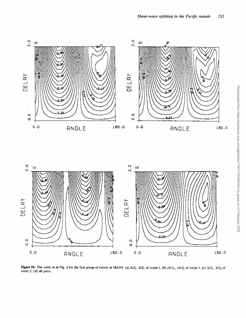
Figure 10. The same as in Fig. 4 for the first group of events at MAJO. (a) ScS,, ScS, of event 1 , (b) sScS,, sSCS, of event 1, (c) ScS, , ScS, of event 2, (d) all pairs.

Dow




5 . 19. 30.00 1 I I . I 20 2p I 22 5 . 3 4 . 30.00 35 I36 37

KIP Event 1 sc s3 KIP Event 1 sc s2

Figure 11. The same as in Fig. 3 for KIP. (a) ScS, of event 1, (b) ScS, of event 1.

0

N

>- a

n w

0

0

180 .o R N G L E 0 .o

Figure U. Plot of E ( a , st) for ScS,, ScS, of event 1 at KIP.

Dow




7 . ‘59. 0.00 1 I I 8. 1 5 . 0 . 0 0 I I . 59 60 I 6p 62 15 I F I 17 18

sc s 2 SCSl ZOBO Event 1 ZOBO Event 1

(4 0 I

(a 0 I

L

I I . 1 . 1 I 12 I 13 8. 15. 0.00 2 2 . 10. 0.00 I5 .’ I F I 17 16 Ib I I

ZOBO Event 1 S C S 2 ZOBO Event 2 SCSl

(e) 0

- L, b-----r?- t -

-250

M

Dow




9 (4 N

>-

3 W 0

a

0 - 0 . 2 6

I i

0 .o FlNGLE 0

cu

>-

_J

w 0

a

0

c\I

>

J w 0

a

0

0

FlNGLE 180.0 0 .o 180 .o

0

0 0.16 > 1

180.0 R N G L E 0 .o

Figure 14. The same as in Fig. 4 for ZOBO. (a) ScS,, ScS, of event 1, (b) ScS,, ScS, of event 2, (c) both pairs.

0 LONG IT UDE m+-' 7

9 120.00 180.00 240.00 * 300.00

\ - .\

l i I I 1

Figure 15. Directions of polarization of the fast split wave (arrows) superimposed on the map of S-wave azimuthal anisotropy at 200 km depth derived from the surface wave data (modified from Montagner & Tanimoto 1991).

Dow




effect of these anisotropies is large (around 1.5 s), probably owing to their similar orientations.

All our estimates of polarization of the fast split wave are summarized in Fig. 15 where they are superimposed on the fast directions at 200 km depth inferred from the phase velocities of the long-period surface waves (Montagner & Tanimoto 1991). Between the two kinds of data there are discrepancies, especially pronounced in the south-west of the study region. Among the possible reasons for the discrepancies, the difference between the corresponding lateral resolutions is probably the most important. Further improvements in the data and techniques are necessary to resolve more details of the mantle flow within and around the Pacific.

ACKNOWLEDGMENT

The study was carried out during the visit of one of the authors (L.V.) to Institut de Physique du Globe de Paris and he thanks R. Madariaga and his staff for their hospitality. The authors appreciate help from J.-P. Montagner and A. Deschamps. Many records used in the study were obtained from NEIC and IRIS data centres, and the authors thank M. Zirbes and T. Ahern for their cooperation.

REFERENCES

Ando, M., 1984. ScS polarization anisotropy around the Pacific ocean, 1. Phys. Earth, 32, 179-195.

Ansel, V. & Nataf, H.C., 1990. On the use of Sc& phases for studying mantle anisotropy, Ann. Geophys., Special Issue (abstract), presented at the EGS 25th General Assembly in Copenhagen, 1990 April 23-27.

Babuska, V. & Cara, M., 1991. Seismic Anisotropy in the Earth, Kluwer, Dordrecht.

Bibee, L. & Shor, G.. Jr, 1976. Compressional wave anisotropy in the crust and upper mantle, Geophys. Res. Lett., 3, 639-642.

Bowman, J.R. & Ando, M., 1987. Shear-wave splitting in the upper-mantle wedge above the Tonga subduction zone, Geophys. J . R. astr. SOC., 88, 25-41.

Cara, M. & Leveque, J.J., 1988. Anisotropy in the asthenosphere: the higher mode data of the Pacific revisited, Geophys. Res. Lett., 11, 633-636.

Chan, W.W. & Der, Z.A., 1988. Attenuation of multiple ScS in various parts of the world, Geophys. J. Int., 92, 303-314.

Christensen, N.I., 1984. The magnitude, symmetry and origin of upper mantle anisotropy based on fabric analyses of ultramafic tectonites, Geophys. J. R. astr. Soc., 76, 89-111.

Chung, T.W., 1992. A quantitative study of seismic anisotropy in the Yamato Basin, the southeastern Japan sea, from refraction data collected by an ocean bottom seismographic array, Geophys. J. Int., 109, 620-638.

Forsyth, D.W., 1975. The early structural evolution and anisotropy of the oceanic upper mantle, Geophys. J . R. astr. SOC., 43,

Fukao, Y., 1984. ScS evidence for anisotropy in the Earth’s mantle, Nature, 309, 695-698.

Hess, H., 1964. Seismic anisotropy of the uppermost mantle under oceans, Nature, 203, 629-631.

Isaccs, B.L., 1988. Uplift of the central Andean plateau and bending of the Bolivian orocline, J. geophys Res., 93,

Jolivet, L., Huchon, P. & Rangin, C., 1989. Tectonic setting of

103-162.

321 1-3231.

Western Pacific marginal basins, Tectonophysics, 160, 23-47. Jolivet, L., Huchon, P., Brunm, J.P., Le Pichon, X.,

Chamrot-Rooke, N. & Thomas, J.C., 1991. Arc deformation and marginal basin opening: Japan Sea as a case study, 1. geophys. Res., %, 4367-4384.

Kravtsov, Yu. A. & Orlov, Yu. I., 1990. Geometrical Optics of Inhomogeneous Media, Springer Verlag, Berlin.

Kuo, B.-Y. & Forsyth, D.W., 1992. A search for split SKS waveforms in the North Atlantic, Geophys. J. Int., 108, 557-574.

Lay, T. & Young, C.J., 1991. Analysis of seismic SV waves in the core’s penumbra, Geophys. Res. Lett., 18, 1373-1376.

Makeyeva, L.I., Vinnik, L.P. & Roecker, S.W., 1992. Shear-wave splitting and small-scale convection in the continental upper mantle, Nature, 358, 144-146.

Malahoff, A, , Feden, R.H. & Fleming, H.S., 1982. Magnetic anomalies and tectonic fabrics of marginal basins North of New Zealand, J. geophys. Res., 87, 4109-4125.

McKenzie, D., 1979. Finite deformation during fluid flow, Geophys.

Minster, J.B. & Jordan, T.H., 1978. Present-day plate motions, J. geophys. Res., 83, 5331-5354.

Mitchell, B.J. & Yu, G., 1980. Surface wave dispersion, regionalized velocity models and anisotropy of the Pacific crust and upper mantle, Geophys. J. R. astr. Soc., 63, 497-514.

Montagner, J.P. & Tanimoto, T., 1990. Global anisotropy in the upper mantle inferred from the regionalization of the phase velocities, J . geophys. Res., 95, 4797-4819.

Montagner, J.P. & Tanimoto, T., 1991. Global upper mantle tomography of seismic velocities and anisotropies, J. geophys. Res., %, 20 337-20 351.

Nishimura, C. & Forsyth, D.W., 1988. Rayleigh wave phase velocities in the Pacific with implications for azimuthal anisotropy and lateral heterogeneities, Geophys. J. R. astr.

Nishimura, C. & Forsyth, D.W., 1989. The anisotropic structure of the upper mantle in the Pacific, Geophys. J. lnt., %, 203-229.

Ribe, N.M., 1989. Seismic anisotropy and mantle flow, J. geophys. Res., 94, 4213-4223.

Ribe, N.M., 1992. On the relation between seismic anisotropy and finite strain, J . geophys. Res., 97, 8737-8747.

Sclater, J.G., Parsons, B. & Jaupart, C., 1981. Ocean and continents: similarities and differences in the mechanisms of heat loss, J. geophys. Res., 86, 11 535-11 552.

Shearer, P. & Orcutt, J., 1985. Anisotropy in the oceanic lithosphere-theory and observations from the Ngendei seismic refraction experiment in the south-west Pacific, Geophys. J. R.

Shearer, P. & Orcutt, J.A., 1986. Compressional and shear wave anisotropy in the oceanic lithosphere-the Ngendei seismic refraction experiment, Geophys. J. R. astr. SOC., 87, 967-1003.

Shimamura, H., 1984. Anisotropy in the oceanic lithosphere of the northwestern Pacific basin, Geophys. J . R. astr. SOC., 76,

Silver, P.G. & Chan, W.W., 1991. Shear wave splitting and subcontinental mantle deformation, J. geophys. Res., 96, 16

Sipkin, S.A. & Jordan, T.H., 1980. Regional variations of Qscs, BUN. seism. SOC. Am., 70, 1071-1102.

Tamaki, K., Suyehiro, K., Allan, J., Ingle, J.C. & Pisciotto, K.A., 1992. Tectonic synthesis and implications of Japan sea drilling, Proc. ODP, Sci. Results, 127/128, College Station, TX.

Tanimoto, T. & Anderson, D.L., 1984. Mapping convection in the mantle, Geophys. Res. Lett., 11, 287-290.

Tanimoto, T. & Anderson, D.L., 1985. Lateral heterogeneity and azimuthal anisotropy in the upper mantle: Love and Rayleigh waves 100-250s, J. geophys. Res., 90, 1842-1858.

Vinnik, L.P. & Farra, V., 1992. Multiple-ScS technique for

J . R. as@. SOC., 58,689-715.

SOC., 94,479-501.

mtr. SOC., 80, 493-526.

253-260.

429-16 454.

Dow



218 V . Furra and L . Vinnik

measuring anisotropy in the mantle, Geophys. Res. Lett., 19,

Vinnik, L.P., Kosarev, G.L. & Makeyeva, L.I., 1984. Anisotropy in the lithosphere from the observations of SKS and SKKS, Dokl. Acud. Nuuk SSSR, 278, 1335-1339 (in Russian).

Vinnik, L.P., Farra, V. & Romanowicz, B., 1989a. Azimuthal anisotropy in the Earth from observations of SKS at Geoscope and NARS broadband stations, Bull. seism. SOC. Am., 79,

489-492.

1542- 1558.

Vinnik, L.P., Farra, V. & Romanowicz, B., 1989b. Observational evidence for diffracted SV on the shadow of the Earth’s core, Geophys. Res. Lett., 16, 519-522.

Vinnik, L.P., Kind, R., Kosarev, G.L. & Makeyeva, L.I., 1989c. Azimuthal anisotropy in the lithosphere from observations of long-period S waves, Geophys. J. Int., 99, 549-559.

Vinnik, L.P., Makeyeva, L.I., Milev, A. & Usenko, A. Yu., 1992. Global patterns of azimuthal anisotropy and deformations in the continental mantle, Geophys. J. Int., 111, 433-447.

Dow



Shear-wave splitting in the mantle of the pacific

Documents

Transcript of Shear-wave splitting in the mantle of the pacific