Shawn W. Walker€¦ · Shawn W. Walker LouisianaStateUniversity DepartmentofMathematicsand Center...
74
Introduction to Shape Optimization Shawn W. Walker Louisiana State University Department of Mathematics and Center for Computation and Technology (CCT) IMA Workshop, June 6-10, 2016 Frontiers in PDE-constrained Optimization
Transcript of Shawn W. Walker€¦ · Shawn W. Walker LouisianaStateUniversity DepartmentofMathematicsand Center...

Introduction to Shape Optimization
Shawn W. Walker
Louisiana State UniversityDepartment of Mathematics and
Center for Computation and Technology (CCT)
IMA Workshop, June 6-10, 2016
Frontiers in PDE-constrained Optimization

Introduction Differential Geometry Surface Derivatives Shape Perturbation Examples Gradient Flows Drag Minimization Conclusion
Table of Contents
1 Introduction
2 Differential Geometry
3 Surface Derivatives
4 Shape Perturbation
5 Examples
6 Gradient Flows
7 Drag Minimization
8 Conclusion
Introduction to Shape Optimization S. W. Walker

Introduction Differential Geometry Surface Derivatives Shape Perturbation Examples Gradient Flows Drag Minimization Conclusion
Examples of Shape Optimization
Optimal shape of structures (G.Allaire, et al).
Inverse problems (shape detection).
Image processing.
Flow control.
Minimum drag bodies.
X0 0.2 0.4 0.6 0.8 1 1.2 1.4 1.6 1.8 2
Y
0
0.2
0.4
0.6
0.8
1Streamlines
Introduction to Shape Optimization S. W. Walker

Introduction Differential Geometry Surface Derivatives Shape Perturbation Examples Gradient Flows Drag Minimization Conclusion
Mathematical Statement
Admissible Set:
Let ΩALL be a “hold-all” domain.
Optimization variable is Ω or Γ.
Denote the admissible set by U .U should have a compactness
property.
Cost Functional:
Let J : U → R be a shape
functional.
Ex: J (Ω) =∫
Ω f(x,Ω) dx.
Ex: J (Γ) =∫
Γg(x,Γ) dS(x).
Ω
ΩALL
Γ
ν
Optimization Problem:
Ω∗ = argminΩ∈U
J (Ω), Γ∗ = argminΓ∈U
J (Γ).
Introduction to Shape Optimization S. W. Walker

Introduction Differential Geometry Surface Derivatives Shape Perturbation Examples Gradient Flows Drag Minimization Conclusion
Shape Optimization Example: Drag Minimization
Define Ω = ΩALL \ ΩB.
u = 0
u = ex
u = ex
ν
ν
Ω
ΩB
ΓOΓBΓI
ΓW
ΓW
Navier-Stokes Equations:
(u · ∇)u−∇ · σ = 0, in Ω,
∇ · u = 0, in Ω,
u = 0, on ΓB,
u = ex, on ΓI ,
u = ex, on ΓW ,
σν = 0, on ΓO.
Cost functional: J (Ω) = −ex ·∫
ΓBσ(u, p)ν (drag force).
Newtonian fluid: σ(u, p) := −pI + 2ReD(u), D(u) := ∇u+(∇u)†
2 .
Reynolds number: Re = ρU0Lµ .
Introduction to Shape Optimization S. W. Walker

Introduction Differential Geometry Surface Derivatives Shape Perturbation Examples Gradient Flows Drag Minimization Conclusion
Shape Sensitivity: Simple Example
ν
Ω
∂ΩR
Let Ω be a disk of radius R.
The boundary is ∂Ω with outer normal ν.
Let f = f(x, y) be a smooth function definedeverywhere.
Suppose f also depends on Ω: f = f(x, y; Ω).
Consider the cost functional:
J (Ω) =
∫
Ω
f(x, y; Ω) dx dy
What is the sensitivity of J with respect to changing R?
Polar coordinates: J =∫ 2π
0
∫ R
0f(r, θ;R) r dr dθ.
Differentiate:
d
dRJ =
∫ 2π
0
(
d
dR
∫ R
0
f(r, θ;R) r dr
)
dθ
=
∫ 2π
0
∫ R
0
f ′(r, θ;R) r dr dθ +
∫ 2π
0
f(R, θ;R)Rdθ.
Introduction to Shape Optimization S. W. Walker

Introduction Differential Geometry Surface Derivatives Shape Perturbation Examples Gradient Flows Drag Minimization Conclusion
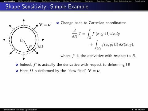
Shape Sensitivity: Simple Example
V = ν
Ω
∂ΩR
Change back to Cartesian coordinates:
d
dRJ =
∫
Ω
f ′(x, y; Ω) dx dy
+
∫
∂Ω
f(x, y; Ω) dS(x, y),
where f ′ is the derivative with respect to R.
Introduction to Shape Optimization S. W. Walker
Introduction Differential Geometry Surface Derivatives Shape Perturbation Examples Gradient Flows Drag Minimization Conclusion
Shape Sensitivity: Simple Example
V = ν
Ω
∂ΩR
Change back to Cartesian coordinates:
d
dRJ =
∫
Ω
f ′(x, y; Ω) dx dy
+
∫
∂Ω
f(x, y; Ω) dS(x, y),
where f ′ is the derivative with respect to R.
Indeed, f ′ is actually the derivative with respect to deforming Ω!
Here, Ω is deformed by the “flow field” V = ν.
Introduction to Shape Optimization S. W. Walker

Introduction Differential Geometry Surface Derivatives Shape Perturbation Examples Gradient Flows Drag Minimization Conclusion
Shape Sensitivity: Simple Example
V = ν
Ω
∂ΩR
Change back to Cartesian coordinates:
d
dRJ =
∫
Ω
f ′(x, y; Ω) dx dy
+
∫
∂Ω
f(x, y; Ω) dS(x, y),
where f ′ is the derivative with respect to R.
Indeed, f ′ is actually the derivative with respect to deforming Ω!
Here, Ω is deformed by the “flow field” V = ν.
We have shown a specific version of a more general formula:
δJ (Ω;V) =
∫
Ω
f ′(x; Ω) dx+
∫
∂Ω
f(x; Ω)V(x) · ν(x) dS(x),
where V is the instantaneous velocity deformation of Ω.
Introduction to Shape Optimization S. W. Walker

Introduction Differential Geometry Surface Derivatives Shape Perturbation Examples Gradient Flows Drag Minimization Conclusion
Notation!
Vectors: e.g. x = (x, y, z)†, a = (a1, a2, a3)†, etc., are column
vectors.
Gradients are row vectors:
∇x =
(∂
∂x,∂
∂y,∂
∂z
)
,
∇x =
(∂
∂x1,
∂
∂x2,
∂
∂x3
)
,
where x = (x, y, z)† or x = (x1, x2, x3)†.
Introduction to Shape Optimization S. W. Walker
Introduction Differential Geometry Surface Derivatives Shape Perturbation Examples Gradient Flows Drag Minimization Conclusion
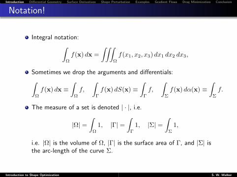
Notation!
Integral notation:
∫
Ω
f(x) dx =
∫∫∫
Ω
f(x1, x2, x3) dx1 dx2 dx3,
Sometimes we drop the arguments and differentials:
∫
Ω
f(x) dx ≡∫
Ω
f,
∫
Γ
f(x) dS(x) ≡∫
Γ
f,
∫
Σ
f(x) dα(x) ≡∫
Σ
f.
The measure of a set is denoted | · |, i.e.
|Ω| =∫
Ω
1, |Γ| =∫
Γ
1, |Σ| =∫
Σ
1,
i.e. |Ω| is the volume of Ω, |Γ| is the surface area of Γ, and |Σ| isthe arc-length of the curve Σ.
Introduction to Shape Optimization S. W. Walker
Introduction Differential Geometry Surface Derivatives Shape Perturbation Examples Gradient Flows Drag Minimization Conclusion
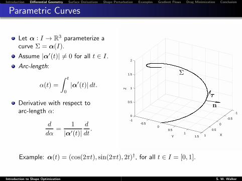
Parametric Curves
Let α : I → R3 parameterize a
curve Σ = α(I).
Assume |α′(t)| 6= 0 for all t ∈ I.
Arc-length:
α(t) =
∫ t
0
|α′(t)| dt.
Derivative with respect toarc-length α:
d
dα=
1
|α′(t)|d
dt.
-10
-0.5-1
0.5
-0.5
X
1
0Z
Y
0
1.5
0.5
2
0.51
11.5
τ
n
Σ
Example: α(t) = (cos(2πt), sin(2πt), 2t)†, for all t ∈ I = [0, 1].
Introduction to Shape Optimization S. W. Walker

Introduction Differential Geometry Surface Derivatives Shape Perturbation Examples Gradient Flows Drag Minimization Conclusion
Parametric Curves
Tangent vector:
τ (t) :=α
′(t)
|α′(t)| , or τ =dα
dα.
Curvature vector:
kn := −d2α
dα2= −dτ
dα,
where n is the unit normal vector.
k is the signed curvature.
Formula in terms of t:
-10
-0.5-1
0.5
-0.5
X
1
0Z
Y
0
1.5
0.5
2
0.51
11.5
τ
n
Σ
k(t)n(t) = − 1
|α′(t)|
(α
′(t)
|α′(t)|
)′
= − α′′(t)
α′(t) ·α′(t)−(
1
|α′(t)|
)′
τ (t)
Introduction to Shape Optimization S. W. Walker

Introduction Differential Geometry Surface Derivatives Shape Perturbation Examples Gradient Flows Drag Minimization Conclusion
Mappings
−2
0
2
−2
0
2−2
−1
0
1
2
−2
0
2
−2
0
2−2
−1
0
1
2
−2
0
2
−2
0
2−2
−1
0
1
2
(a) Ellipsoidal Set (b) Rotated Set (c) Deformed Set
x1x1x1 x2x2x2
x3
x3
x3
A mapping Φ = (Φ1,Φ2,Φ3)† can be viewed as a deformation.
Ex: (b) rigid motion: Φ(x) = Rx+ b.
Ex: (c) Φ(x) = (x1 − 1.2 + 1.6 cos(x3π/4), x2, x3)†.
Introduction to Shape Optimization S. W. Walker

Introduction Differential Geometry Surface Derivatives Shape Perturbation Examples Gradient Flows Drag Minimization Conclusion
Parametric Representation of a Surface
Think of creating a surface by deforming a flat rubber sheet into acurved sheet.
Let U ⊂ R2 be a “flat” domain (reference domain).
Let X : U → R3 be the
parameterization.
(s1, s2)† in U are the parameters.
Every point x = (x1, x2, x3)† in R
3
is given by
x = X(s1, s2).
Γ = X(U) denotes the surfaceobtained from “deforming” U .
−1
0
1
2 −1
0
1
2
3
0
0.5
1
1.5
2
2.5
3
x1
x2
x3
X
U
Γ
Introduction to Shape Optimization S. W. Walker

Introduction Differential Geometry Surface Derivatives Shape Perturbation Examples Gradient Flows Drag Minimization Conclusion
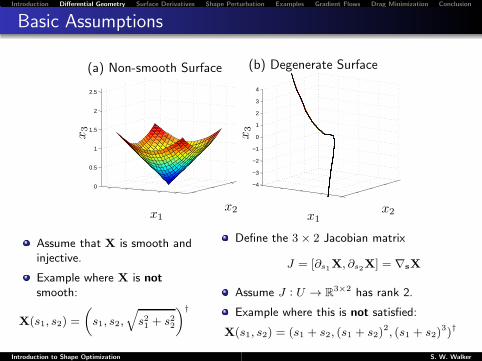
Basic Assumptions
0
0.5
1
1.5
2
2.5
−4
−3
−2
−1
0
1
2
3
4
(a) Non-smooth Surface (b) Degenerate Surface
x1x1x2x2
x3
x3
Introduction to Shape Optimization S. W. Walker
Introduction Differential Geometry Surface Derivatives Shape Perturbation Examples Gradient Flows Drag Minimization Conclusion
Basic Assumptions
0
0.5
1
1.5
2
2.5
−4
−3
−2
−1
0
1
2
3
4
(a) Non-smooth Surface (b) Degenerate Surface
x1x1x2x2
x3
x3
Assume that X is smooth andinjective.
Example where X is notsmooth:
X(s1, s2) =
(
s1, s2,
√
s21 + s22
)†
Define the 3× 2 Jacobian matrix
J = [∂s1X, ∂s2X] = ∇sX
Assume J : U → R3×2 has rank 2.
Example where this is not satisfied:
X(s1, s2) = (s1 + s2, (s1 + s2)2, (s1 + s2)
3)†
Introduction to Shape Optimization S. W. Walker

Introduction Differential Geometry Surface Derivatives Shape Perturbation Examples Gradient Flows Drag Minimization Conclusion
Parameterization of a Plane
−2−1
01
2
−2
0
2
−2
−1
0
1
2
−2−1
01
2
−2
0
2
−2
−1
0
1
2
x1x1 x2x2
x3
x3
(a) Cartesian parameterization (b) Polar coordinates
Plane: x ∈ R3 : x ·N = 0, N = (N1, N2, N3)
†.Solve for x3: x3 = −1
N3(x1N1 + x2N2).
(a) X(s1, s2) =(
s1, s2,−s1N1+s2N2
N3
)†
, for all (s1, s2)† in U , where
U = R2.
(b) X(r, θ) =(
r cos θ, r sin θ,−r cos θN1+sin θN2
N3
)†
, where
U = (0,∞)× (0, 2π).
Introduction to Shape Optimization S. W. Walker

Introduction Differential Geometry Surface Derivatives Shape Perturbation Examples Gradient Flows Drag Minimization Conclusion
Regular Surface; Local Charts
A regular surface is built from many maps and reference domains(U,X).
We call (U,X) a local chart.
For a general surface, one needs an atlas of local charts: (Ui,Xi).
x1
x2
x3
s1
s2
U1U2
U3
Γ
X
X
X
Introduction to Shape Optimization S. W. Walker
Introduction Differential Geometry Surface Derivatives Shape Perturbation Examples Gradient Flows Drag Minimization Conclusion
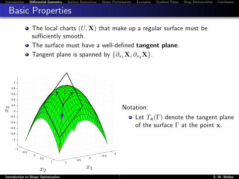
Basic Properties
The local charts (U,X) that make up a regular surface must besufficiently smooth.
The surface must have a well-defined tangent plane.
Tangent plane is spanned by ∂s1X, ∂s2X.
−1−0.5
00.5
1
−1−0.5
00.5
1
−1
−0.8
−0.6
−0.4
−0.2
0
0.2
0.4
0.6
0.8
1
x1x2
x3 Notation:
Let Tx(Γ) denote the tangent planeof the surface Γ at the point x.
Introduction to Shape Optimization S. W. Walker

Introduction Differential Geometry Surface Derivatives Shape Perturbation Examples Gradient Flows Drag Minimization Conclusion
First Fundamental Form
Deforming the reference domain distorts it.
Need a characterization of the distortion.
Define the coefficients of the First Fundamental Form:
gij = ∂siX · ∂sjX, for 1 ≤ i, j ≤ 2.
10.5
0-0.5
-1-1
-0.5
0
0.5
0.5
0
-0.5
-1
1
1
0.50
-0.5-1-1
-0.5
0
0.5
-1
-0.5
0
0.5
1
1
x1x1 x2x2
x3
x3
(a) Top-Half Of Unit Sphere (b) Side-Half Of Unit Sphere
Introduction to Shape Optimization S. W. Walker

Introduction Differential Geometry Surface Derivatives Shape Perturbation Examples Gradient Flows Drag Minimization Conclusion
Example: Plane
Recall the cartesian parameterization of a plane:
X(s1, s2) =(
s1, s2,− s1N1+s2N2
N3
)†
.
Compute: ∂s1X =(
1, 0,−N1
N3
)†
, ∂s2X =(
0, 1,−N2
N3
)†
.
First fundamental form coefficients are:
g11 = ∂s1X · ∂s1X = 1 + (N1/N3)2,
g12 = ∂s1X · ∂s2X = g21 = (N1/N3)(N2/N3),
g22 = ∂s2X · ∂s2X = 1 + (N2/N3)2,
which are all constant.
Introduction to Shape Optimization S. W. Walker

Introduction Differential Geometry Surface Derivatives Shape Perturbation Examples Gradient Flows Drag Minimization Conclusion
Example: Sphere
Consider the parameterization of part of a sphere:
(x1, x2, x3)† ∈ R
3 : x21 + x2
2 + x23 = 1.
Top-half: X1(s1, s2) =(
s1, s2,+√
1− (s21 + s22))†
,
for all (s1, s2)† in U = (s1, s2)† ∈ R
2 : s21 + s22 < 1.
Compute: ∂s1X(s1, s2) =(
1, 0,−s1(1− (s21 + s22))−1/2
)†
,
∂s2X(s1, s2) =(
0, 1,−s2(1− (s21 + s22))−1/2
)†
.
First fundamental form coefficients are:
g11 = ∂s1X · ∂s1X =1− s22
1− (s21 + s22),
g12 = ∂s1X · ∂s2X = g21 =s1s2
1− (s21 + s22),
g22 = ∂s2X · ∂s2X =1− s21
1− (s21 + s22),
which blow-up as (s21 + s22) → 1.
Introduction to Shape Optimization S. W. Walker

Introduction Differential Geometry Surface Derivatives Shape Perturbation Examples Gradient Flows Drag Minimization Conclusion
Metric Tensor
The coefficients gij can be grouped into a 2× 2 matrix denoted g:
g =
[g11 g12g21 g22
]
= (∇sX)†(∇sX),
which is a symmetric matrix because g12 = g21.g is positive definite for a regular surface.The inverse matrix:
g−1 =
[g11 g12
g21 g22
]
=1
det(g)
[g22 −g12−g21 g11
]
;
note the superscript indices.Of course, we have the following property because g g−1 = I:
δij =
2∑
k=1
gikgkj =
2∑
k=1
gikgjk,
where δij is the “Kronecker delta”:
δij =
0, if i 6= j,1, if i = j.
Introduction to Shape Optimization S. W. Walker

Introduction Differential Geometry Surface Derivatives Shape Perturbation Examples Gradient Flows Drag Minimization Conclusion
Normal Vector
If X parameterizes a surface, then the normal vector ν is given by
ν(s) = ν(s1, s2) =∂s1X(s)× ∂s2X(s)
|∂s1X(s)× ∂s2X(s)| =∂s1X(s)× ∂s2X(s)√
det g
Choice of parameterization induces an orientation of the surface.
−2
−1
0
1
2 −2−1
01
2
−2
−1
0
1
2
−3 −2 −1 0 1 2 3−3
−2
−1
0
1
2
3
−3
−2
−1
0
1
2
3
x1
x1 x2x2
x3
x3
(a) Orientable (b) Non-orientable
Introduction to Shape Optimization S. W. Walker

Introduction Differential Geometry Surface Derivatives Shape Perturbation Examples Gradient Flows Drag Minimization Conclusion
Surface Area
Let (U,X) be a local chart of Γ, with R = X(U) ⊂ Γ.
The area of R is given by
|R| :=∫
R
1 =
∫∫
U
|∂s1X×∂s2X| ds1 ds2 =
∫∫
U
√
det g(s1, s2) ds1 ds2,
where g = g(s1, s2) is the metric tensor.
Standard change of variable formula for surface integrals.
Introduction to Shape Optimization S. W. Walker

Introduction Differential Geometry Surface Derivatives Shape Perturbation Examples Gradient Flows Drag Minimization Conclusion
Deviating From The Tangent Plane
Curved surface Γ.
Tangent plane TP (Γ) in green.
Let P = X(s1, s2) andQ = X(s1 + ℓ1, s2 + ℓ2).
distance: dist(Q, TP (Γ)) =
1
2
2∑
i,j=1
ℓiℓj ∂si∂sjX · ν︸ ︷︷ ︸
=hij
+ H.O.T.
where ν is the normal vector of Γat P .
−1−0.5
00.5
1−1
−0.5
0
0.5
1
−1
−0.8
−0.6
−0.4
−0.2
0
0.2
0.4
0.6
0.8
1
x1
x2
x3
P
Q
hij are the coefficients of the second fundamental form.
Introduction to Shape Optimization S. W. Walker

Introduction Differential Geometry Surface Derivatives Shape Perturbation Examples Gradient Flows Drag Minimization Conclusion
Second Fundamental Form
Define the coefficients of the second fundamental form:
hij = ν · ∂si∂sjX, for 1 ≤ i, j ≤ 2,
Since ν · ∂sjX = 0 for j = 1, 2, we can differentiate to see that
∂siν · ∂sjX+ ν · ∂si∂sjX = 0, for 1 ≤ i, j ≤ 2.
Hence, we can write
hij = −∂siν · ∂sjX = ν · ∂si∂sjX, for 1 ≤ i, j ≤ 2.
The coefficients hij can be grouped into a 2× 2 matrix denoted h:
h =
[h11 h12
h21 h22
]
,
which is a symmetric matrix because h12 = h21.
h is not necessarily positive definite.
Alternative formula:
h = −(∇sν)†(∇sX).
Introduction to Shape Optimization S. W. Walker
Introduction Differential Geometry Surface Derivatives Shape Perturbation Examples Gradient Flows Drag Minimization Conclusion
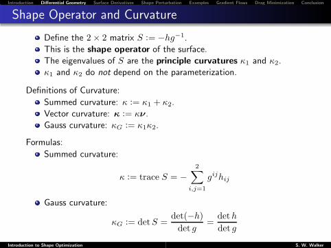
Shape Operator and Curvature
Define the 2× 2 matrix S := −hg−1.
This is the shape operator of the surface.
The eigenvalues of S are the principle curvatures κ1 and κ2.
κ1 and κ2 do not depend on the parameterization.
Introduction to Shape Optimization S. W. Walker
Introduction Differential Geometry Surface Derivatives Shape Perturbation Examples Gradient Flows Drag Minimization Conclusion
Shape Operator and Curvature
Define the 2× 2 matrix S := −hg−1.
This is the shape operator of the surface.
The eigenvalues of S are the principle curvatures κ1 and κ2.
κ1 and κ2 do not depend on the parameterization.
Definitions of Curvature:
Summed curvature: κ := κ1 + κ2.
Vector curvature: κ := κν.
Gauss curvature: κG := κ1κ2.
Formulas:
Summed curvature:
κ := trace S = −2∑
i,j=1
gijhij
Gauss curvature:
κG := detS =det(−h)
det g=
deth
det g
Introduction to Shape Optimization S. W. Walker

Introduction Differential Geometry Surface Derivatives Shape Perturbation Examples Gradient Flows Drag Minimization Conclusion
Classification of Surfaces
−1
0
1
−10
1
−1
−0.5
0
0.5
1
1.5
2
−1
0
1
−10
1
−1
−0.5
0
0.5
1
1.5
2
−1
0
1
−10
1
−1
−0.5
0
0.5
1
1.5
2
x1x1x1 x2x2x2
x3
x3
x3
(a) Elliptic (κG > 0) (b) Parabolic (κG = 0) (c) Hyperbolic (κG < 0)
The Gauss curvature provides a way to classify (qualitatively) localsurface geometry.
Introduction to Shape Optimization S. W. Walker

Introduction Differential Geometry Surface Derivatives Shape Perturbation Examples Gradient Flows Drag Minimization Conclusion
Functions on Surfaces
−1
−0.5
0
0.5
1 −1
−0.5
0
0.5
1
−1
−0.5
0
0.5
1
−1 −0.5 0 0.5 1
−1
−0.5
0
0.5
1 −1
−0.5
0
0.5
1
−1
−0.5
0
0.5
1
−1 −0.5 0 0.46
x1x1x2x2
x3
x3
(a) f1 (b) f2
Let f : Γ → R be a function defined on Γ.
If (U,X) is a local chart, then define f := f X : U → R.
We say f is smooth i.f.f. f is smooth in the usual sense.
In practice, we first define f : U → R, then form f := f X−1.
Introduction to Shape Optimization S. W. Walker
Introduction Differential Geometry Surface Derivatives Shape Perturbation Examples Gradient Flows Drag Minimization Conclusion
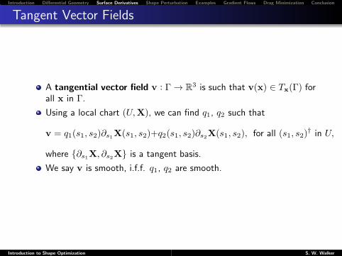
Tangent Vector Fields
A tangential vector field v : Γ → R3 is such that v(x) ∈ Tx(Γ) for
all x in Γ.
Using a local chart (U,X), we can find q1, q2 such that
v = q1(s1, s2)∂s1X(s1, s2)+q2(s1, s2)∂s2X(s1, s2), for all (s1, s2)† in U,
where ∂s1X, ∂s2X is a tangent basis.
We say v is smooth, i.f.f. q1, q2 are smooth.
Introduction to Shape Optimization S. W. Walker

Introduction Differential Geometry Surface Derivatives Shape Perturbation Examples Gradient Flows Drag Minimization Conclusion
Tangential Directional Derivative
Let ω : Γ → R be a surface function.
Denote the tangential directional derivative of ω at P in Γ, in thedirection v in TP (Γ), by Dvω(P ).
Suppose α(t) is a parameterization of acurve (red) contained in Γ such thatα(0) = P and α
′(0) = v (blue), then
Dvω(P ) :=d
dtω(α(t))
∣∣∣t=0
−1−0.5
00.5
1
−1−0.5
00.5
1
−1
−0.8
−0.6
−0.4
−0.2
0
0.2
0.4
0.6
0.8
1
x1x2
x3
Introduction to Shape Optimization S. W. Walker

Introduction Differential Geometry Surface Derivatives Shape Perturbation Examples Gradient Flows Drag Minimization Conclusion
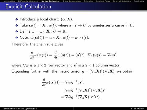
Explicit Calculation
Introduce a local chart: (U,X).
Take α(t) = X s(t), where s : I → U parameterizes a curve in U .
Define ω = ω X : U → R.
Note: ω(α(t)) = ω X s(t) = ω s(t).
Introduction to Shape Optimization S. W. Walker

Introduction Differential Geometry Surface Derivatives Shape Perturbation Examples Gradient Flows Drag Minimization Conclusion
Explicit Calculation
Introduce a local chart: (U,X).
Take α(t) = X s(t), where s : I → U parameterizes a curve in U .
Define ω = ω X : U → R.
Note: ω(α(t)) = ω X s(t) = ω s(t).Therefore, the chain rule gives
d
dtω(α(t)) =
d
dtω(s(t)) = (s′(t) · ∇s)ω(s) = ∇ωs′,
where ∇ω is a 1× 2 row vector and s′ is a 2× 1 column vector.
Introduction to Shape Optimization S. W. Walker
Introduction Differential Geometry Surface Derivatives Shape Perturbation Examples Gradient Flows Drag Minimization Conclusion
Explicit Calculation
Introduce a local chart: (U,X).
Take α(t) = X s(t), where s : I → U parameterizes a curve in U .
Define ω = ω X : U → R.
Note: ω(α(t)) = ω X s(t) = ω s(t).Therefore, the chain rule gives
d
dtω(α(t)) =
d
dtω(s(t)) = (s′(t) · ∇s)ω(s) = ∇ωs′,
where ∇ω is a 1× 2 row vector and s′ is a 2× 1 column vector.
Expanding further with the metric tensor g = (∇sX)†(∇sX), we obtain
d
dtω(α(t)) = ∇ωg−1gs′,
= ∇ωg−1(∇sX)†(∇sX)s′
= ∇ωg−1(∇sX)†α′(t).
Introduction to Shape Optimization S. W. Walker

Introduction Differential Geometry Surface Derivatives Shape Perturbation Examples Gradient Flows Drag Minimization Conclusion
Surface Gradient Operator
Hence, we obtain
d
dtω(α(t))
∣∣∣t=0
= ∇ωg−1(∇sX)†α′(t)∣∣∣t=0
⇒ Dvω(P ) = ∇ωg−1(∇sX)†︸ ︷︷ ︸
1×3 row vector
· v.
In general,
Dvω X = ∇ωg−1(∇sX)† · v, for arbitrary v,
evaluated at s with P = X(s).
Denote the surface gradient of ω at P in Γ by ∇Γω(P ) in TP (Γ).
Define it by ∇Γω(P ) · v = Dvω(P ), for all v ∈ TP (Γ).
Thus,
(∇ΓωX)·v = DvωX = ∇ωg−1(∇sX)†·v, for all v ∈ TX(s)(Γ).
Therefore, ∇Γω X = ∇sωg−1(∇sX)†.
Introduction to Shape Optimization S. W. Walker

Introduction Differential Geometry Surface Derivatives Shape Perturbation Examples Gradient Flows Drag Minimization Conclusion
Surface Gradient Example
−1
−0.5
0
0.5
1 −1
−0.5
0
0.5
1
−1
−0.5
0
0.5
1
−1
−0.5
0
0.5
1 −1
−0.5
0
0.5
1
−1
−0.5
0
0.5
1
x1x1x2x2
x3
x3
(a) ∇Γf1 (b) ∇Γf2
If ϕ = (ϕ1, ϕ2, ϕ3), then
(∇Γϕ) X =
(∇Γϕ1) X(∇Γϕ2) X(∇Γϕ3) X
, a 3× 3 matrix.
Introduction to Shape Optimization S. W. Walker

Introduction Differential Geometry Surface Derivatives Shape Perturbation Examples Gradient Flows Drag Minimization Conclusion
Other Surface Operators; Curvatures
Surface Operators:
Identity map: idΓ(x) = x for all x in Γ.
Tangent space projection: ∇ΓidΓ = I− ν ⊗ ν.
Surface divergence: ∇Γ ·ϕ = trace(∇Γϕ).
Surface Laplacian (Laplace-Beltrami): ∆Γω := ∇Γ · ∇Γω.
Alternate curvature formulas:
Curvature vector: −∆ΓidΓ = κν.
Gauss curvature:
κG = ν · ∂s1ν × ∂s2ν√
det(g), κGν =
∂s1ν × ∂s2ν√
det(g).
Surface divergence of the normal vector: ∇Γ · ν = κ.
Introduction to Shape Optimization S. W. Walker

Introduction Differential Geometry Surface Derivatives Shape Perturbation Examples Gradient Flows Drag Minimization Conclusion
Integration by Parts on Surfaces
Let Γ be a surface with boundary ∂Γ.
ν is the oriented normal vector of Γ.
τ is the positively oriented tangent vector of ∂Γ.
Let ω : Γ → R be differentiable.
Integration by parts:
∫
Γ
∇Γω =
∫
Γ
ωκν +
∫
∂Γ
ω(τ × ν)
(τ × ν) is the “outer normal” of the boundary ∂Γ.
Another integration by parts formula:
∫
Γ
∇Γϕ · ∇Γη = −∫
Γ
ϕ∆Γη +
∫
∂Γ
ϕ(τ × ν) · ∇Γη,
where ϕ, η : Γ → R are differentiable.
Introduction to Shape Optimization S. W. Walker

Introduction Differential Geometry Surface Derivatives Shape Perturbation Examples Gradient Flows Drag Minimization Conclusion
Shape Functionals
Recall shape functionals:
E(Ω) =∫
Ω
f(x,Ω), J (Γ) =
∫
Γ
f(x,Ω), B(Γ) =∫
Γ
g(x,Γ).
Note: Γ ⊂ Ω.
Application: optimization.
Ω∗ = argminΩ
E(Ω), Γ∗ = argminΓ
J (Γ), Γ∗ = argminΓ
B(Γ).
Introduction to Shape Optimization S. W. Walker

Introduction Differential Geometry Surface Derivatives Shape Perturbation Examples Gradient Flows Drag Minimization Conclusion
Perturbing the Domain
x1
x2 x3
x4x′1
x′2
x′3
x′4
ǫV ǫV
Ω Ωǫ
Γ
Γǫ
Perturbation of the identity:
Mapping the bulk domain:
Φǫ(x) := x+ ǫV(x), for all x in ΩALL,
where Ωǫ = Φǫ(Ω).
Mapping an embedded surface:
Xǫ X−1(x) := x+ ǫV(x), for all x in Γ ⊂ ΩALL,
where Γǫ = Xǫ X−1(Γ).
Introduction to Shape Optimization S. W. Walker

Introduction Differential Geometry Surface Derivatives Shape Perturbation Examples Gradient Flows Drag Minimization Conclusion
Perturbing Functions
Material derivative:
f(Ω;V)(x) ≡ f(x) := limǫ→0
fǫ(Φǫ(x)) − f(x)
ǫ, for all x in Ω,
Extend f to all of ΩALL such that
fǫ(Φǫ(x)) = f(ǫ,Φǫ(x)), for all x ∈ Ω, ǫ ∈ [0, ǫmax].
Differentiate:
f(x) =d
dǫf(ǫ,Φǫ(x))
∣∣∣ǫ=0
=∂
∂ǫf(0,x) +∇f(0,x) · d
dǫΦǫ(x)
∣∣∣ǫ=0
=∂
∂ǫf(0,x)
︸ ︷︷ ︸
=:f ′(Ω;V)(x)
+(V(x) · ∇) f(0,x)︸ ︷︷ ︸
=f(x)
.
Shape derivative: f ′(x) ≡ f ′(Ω;V)(x).
Introduction to Shape Optimization S. W. Walker

Introduction Differential Geometry Surface Derivatives Shape Perturbation Examples Gradient Flows Drag Minimization Conclusion
Perturbing Functions
Relationship between material derivative and shape derivatives:
Perturbing functions f defined on Ω:
f(x) = f ′(x) +V(x) · ∇f(x)
Perturbing functions g defined on Γ:
g(x) = g′(x) +V(x) · ∇Γg(x)
Other examples:
Local perturbation of Γ:
˙idΓ = V, id′Γ = (V · ν)ν
Perturb the normal vector:
ν = −(∇ΓV)†ν, ν′ = −∇Γ (V · ν)†
Perturb the summed curvature:
κ = −ν · (∆ΓV)− 2(∇ΓV) : (∇Γν), κ′ = −∆Γ (V · ν)
Introduction to Shape Optimization S. W. Walker

Introduction Differential Geometry Surface Derivatives Shape Perturbation Examples Gradient Flows Drag Minimization Conclusion
Perturbing Functionals
Consider the perturbed functionals:
Eǫ =∫
Ωǫ
f(Ωǫ), Jǫ =
∫
Γǫ
f(Ωǫ), Bǫ =
∫
Γǫ
g(Γǫ), for all ǫ ≥ 0,
and define the corresponding shape perturbations:
δE(Ω) ·V ≡ δE(Ω;V) :=d
dǫEǫ∣∣∣ǫ=0+
,
δJ (Γ) ·V ≡ δJ (Γ;V) :=d
dǫJǫ
∣∣∣ǫ=0+
,
δB(Γ) ·V ≡ δB(Γ;V) :=d
dǫBǫ
∣∣∣ǫ=0+
.
Introduction to Shape Optimization S. W. Walker

Introduction Differential Geometry Surface Derivatives Shape Perturbation Examples Gradient Flows Drag Minimization Conclusion
Perturbing Functionals
δE(Ω;V) =
∫
Ω
f(Ω;V) +
∫
Ω
f(Ω)(∇ ·V) =
recall intro. example︷ ︸︸ ︷∫
Ω
f ′(Ω;V) +
∫
∂Ω
f(Ω)(V · ν),
δJ (Γ;V) =
∫
Γ
f(Ω;V) + f(∇Γ ·V)
=
∫
Γ
f ′(Ω;V) + (V · ∇)f + f(∇Γ ·V)
=
∫
Γ
f ′(Ω;V) +[(ν · ∇)f + fκ
](V · ν) +
∫
∂Γ
f(τ × ν) ·V,
δB(Γ;V) =
∫
Γ
g(Γ;V) + g(∇Γ ·V)
=
∫
Γ
g′(Γ;V) + (V · ∇Γ)g + g(∇Γ ·V)
=
∫
Γ
g′(Γ;V) + gκ(V · ν) +∫
∂Γ
g(τ × ν) ·V.
Introduction to Shape Optimization S. W. Walker

Introduction Differential Geometry Surface Derivatives Shape Perturbation Examples Gradient Flows Drag Minimization Conclusion
Structure Theorem
Hadamard-Zolesio structure theorem.
Ω is a “flat” domain.
Let J = J (Ω) be a generic shape functional, whose shapeperturbation exists.
If everything is sufficiently smooth, then one can always write
δJ (Ω;V) =
∫
∂Ω
η(V · ν),
for some function η in L1(∂Ω).
Example:
δE(Ω;V) =
∫
Ω
f ′(Ω;V) +
∫
∂Ω
f(Ω)(V · ν).
Rewriting∫
Ω f ′(Ω;V) as an integral over ∂Ω requires using anadjoint PDE.
Introduction to Shape Optimization S. W. Walker

Introduction Differential Geometry Surface Derivatives Shape Perturbation Examples Gradient Flows Drag Minimization Conclusion
Minimal Surfaces
10.5
01
0.5
0
0.5
0
10.5
010.5
0.5
00
10.5010.5
0
0.5
0
(a) u = ga, on ∂Ω (b) u = gb, on ∂Ω (c) u = gc, on ∂Ω
xxx yyy
z
Let Γ be a surface with boundary ∂Γ ≡ Σ.
Perimeter functional: J (Γ) =∫
Γ 1 dS.
What is the first order optimality condition?
Apply shape perturbation formula with f = 1:
δJ (Γ;V) =
∫
Γ
f ′ +[(ν · ∇)f + fκ
](V · ν) +
∫
Σ
f(τ × ν) ·V,
=
∫
Γ
κν ·V = 0,
for all smooth perturbations V that vanish on Σ.
First order condition is: κ = 0.Introduction to Shape Optimization S. W. Walker

Introduction Differential Geometry Surface Derivatives Shape Perturbation Examples Gradient Flows Drag Minimization Conclusion
Surface Tension
Γs
ΓΓ
b
bbs
bs
νν
Σ τΣ
θclex
ex
ey
ezez
Γs,g
Let γ be a surface tension coefficient.
Consider the surface energy functional: J (Γ) =∫
Γγ dS(x).
Differentiating the energy gives the “force”:
δJ (Γ;V) =
∫
Γ
γκν ·V +
∫
Σ
γb ·V,
where V is a perturbation of the surface Γ. Note: b = τΣ × ν.
δJ (Γ;V) is the relative force exerted by surface tension againstdeforming the surface by V.
Integral over Σ are the contact line forces.
Introduction to Shape Optimization S. W. Walker

Introduction Differential Geometry Surface Derivatives Shape Perturbation Examples Gradient Flows Drag Minimization Conclusion
Shape Optimization
Consider a shape functional J = J (Γ) defined over a set ofadmissible shapes U .The optimization problem is:
find Γ∗ ∈ U , such that J (Γ∗) = minΓ∈U
J (Γ).
Can we evolve Γ = Γ(t) with a “velocity field” such that
J (Γ(t2)) < J (Γ(t1)), whenever t1 < t2.
Note: “time” here is a pseudotime that corresponds to our flow“velocity.”
Introduction to Shape Optimization S. W. Walker

Introduction Differential Geometry Surface Derivatives Shape Perturbation Examples Gradient Flows Drag Minimization Conclusion
Variational Problem
Define a “velocity” space:
V(Γ) =
V :
∫
Γ
|V|2 < ∞
, with norm ‖V‖V(Γ) :=(∫
Γ
|V|2)1/2
Define a bilinear form b : V(Γ)× V(Γ) → R such thatb(V,Y) =
∫
ΓV ·Y.
Note that ‖V‖V(Γ) =√
b(V,V).
We now define the velocity field as follows: at each time t ≥ 0, findV(t) in V(Γ(t)) that solves the following variational problem:
b(V(t),Y) = −δJ (Γ(t);Y), for all Y ∈ V(Γ(t)).
This ensures we decrease the energy because
δJ (Γ(t);V(t)) = −b(V(t),V(t)) = −‖V(t)‖2V(Γ) < 0.
Introduction to Shape Optimization S. W. Walker

Introduction Differential Geometry Surface Derivatives Shape Perturbation Examples Gradient Flows Drag Minimization Conclusion
L2-Gradient Descent
Discretize time:
Start with an initial domain Γ0.
FOR i = 0, 1, 2, ..., find Vi in V(Γi) such that
b(Vi,Y) = −δJ (Γi;Y), for all Y ∈ V(Γi).
Define perturbation of the identity:
X∆t (Xi)−1(x) := idΓi(x) + ∆tVi(x), for all x in Γi.
where Xi is a parameterization of Γi, and ∆t is a “time-step”.
Update the domain: Γi+1 = X∆t (Xi)−1(Γi).
If the time step ∆t is small enough, then the sequence J (Γi)i≥0
is decreasing, i.e.
J (t0) > J (t1) > J (t2) > · · · > J (ti) > J (ti+1) > · · ·
Choosing a different space V(Γ) can improve the convergence rate.
Introduction to Shape Optimization S. W. Walker

Introduction Differential Geometry Surface Derivatives Shape Perturbation Examples Gradient Flows Drag Minimization Conclusion
Mean Curvature Flow
Assume Γ is a closed surface.
Consider the perimeter functional: J (Γ) =∫
Γ1 dS(x).
For each t ≥ 0, find V(t) such that
∫
Γ(t)
V(t) ·Y = −δJ (Γ(t);Y) = −∫
Γ(t)
κ(t)ν(t) ·Y,
for all smooth perturbations Y.
Continuing, we get∫
Γ(t)
[V(t) + κ(t)ν(t)
]·Y = 0, for all smooth Y.
Therefore, V(t,x) = −κ(t,x)ν(t,x), for all x ∈ Γ(t).
The surface Γ(t) moves with normal velocity:
V · ν = −κ.
Mean curvature flow is the L2-gradient flow of perimeter.
Introduction to Shape Optimization S. W. Walker
Introduction Differential Geometry Surface Derivatives Shape Perturbation Examples Gradient Flows Drag Minimization Conclusion
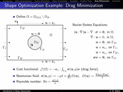
Shape Optimization Example: Drag Minimization
Define Ω = ΩALL \ ΩB.
u = 0
u = ex
u = ex
ν
ν
Ω
ΩB
ΓOΓBΓI
ΓW
ΓW
Navier-Stokes Equations:
(u · ∇)u−∇ · σ = 0, in Ω,
∇ · u = 0, in Ω,
u = 0, on ΓB,
u = ex, on ΓI ,
u = ex, on ΓW ,
σν = 0, on ΓO.
Cost functional: J (Ω) = −ex ·∫
ΓBσ(u, p)ν (drag force).
Newtonian fluid: σ(u, p) := −pI + 2ReD(u), D(u) := ∇u+(∇u)†
2 .
Reynolds number: Re = ρU0Lµ .
Introduction to Shape Optimization S. W. Walker
Introduction Differential Geometry Surface Derivatives Shape Perturbation Examples Gradient Flows Drag Minimization Conclusion
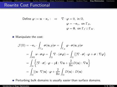
Rewrite Cost Functional
Define ϕ := u− ex : ⇒ ∇ · ϕ = 0, in Ω,
ϕ = −ex, on ΓB,
ϕ = 0, on ΓI ∪ ΓW .
Manipulate the cost:
J (Ω) = −ex ·∫
ΓB
σ(u, p)ν =
∫
ΓB
ϕ · σ(u, p)ν
=
∫
∂Ω
ν · σϕ =
∫
Ω
∇ · (σϕ) =∫
Ω
[∇ · σ] ·ϕ+ σ : ∇ϕ
=
∫
Ω
[∇ · σ] ·ϕ− pI : ∇u+2
ReD(u) : ∇u
=
∫
Ω
[(u · ∇)u] · ϕ+2
Re
∫
Ω
D(u) : D(u)
Perturbing bulk domains is usually easier than surface domains.
Introduction to Shape Optimization S. W. Walker

Introduction Differential Geometry Surface Derivatives Shape Perturbation Examples Gradient Flows Drag Minimization Conclusion
Differentiate The Cost
J (Ω) =
∫
Ω
[(u · ∇)u] ·ϕ+2
Re
∫
Ω
D(u) : D(u)
Apply shape perturbation formula:
δJ (Ω;V) =
∫
Ω
[
(u′ · ∇)u+ (u · ∇)u′]
·ϕ+
∫
Ω
[(u · ∇)u] ·ϕ′
+
∫
∂Ω
(V · ν)[(u · ∇)u] ·ϕ+
+4
Re
∫
Ω
D(u′) : D(u) +2
Re
∫
∂Ω
(V · ν)|D(u)|2
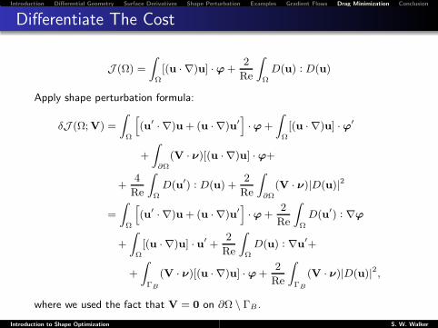
=
∫
Ω
[
(u′ · ∇)u+ (u · ∇)u′]
·ϕ+2
Re
∫
Ω
D(u′) : ∇ϕ
+
∫
Ω
[(u · ∇)u] · u′ +2
Re
∫
Ω
D(u) : ∇u′+
+
∫
ΓB
(V · ν)[(u · ∇)u] · ϕ+2
Re
∫
ΓB
(V · ν)|D(u)|2,
where we used the fact that V = 0 on ∂Ω \ ΓB .
Introduction to Shape Optimization S. W. Walker
Introduction Differential Geometry Surface Derivatives Shape Perturbation Examples Gradient Flows Drag Minimization Conclusion
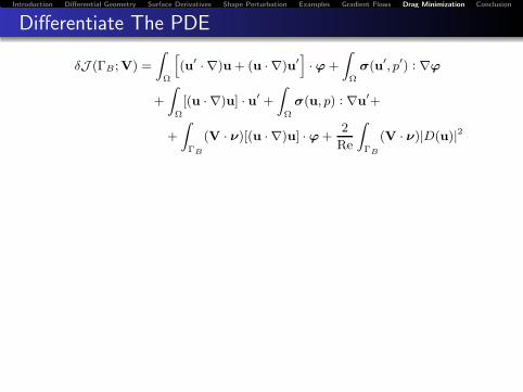
Differentiate The PDE
δJ (ΓB ;V) =
∫
Ω
[
(u′ · ∇)u+ (u · ∇)u′]
·ϕ+
∫
Ω
σ(u′, p
′) : ∇ϕ
+
∫
Ω
[(u · ∇)u] · u′ +
∫
Ω
σ(u, p) : ∇u′+
+
∫
ΓB
(V · ν)[(u · ∇)u] · ϕ+2
Re
∫
ΓB
(V · ν)|D(u)|2

Introduction Differential Geometry Surface Derivatives Shape Perturbation Examples Gradient Flows Drag Minimization Conclusion
Differentiate The PDE
δJ (ΓB ;V) =
∫
Ω
[
(u′ · ∇)u+ (u · ∇)u′]
·ϕ+
∫
Ω
σ(u′, p
′) : ∇ϕ
+
∫
Ω
[(u · ∇)u] · u′ +
∫
Ω
σ(u, p) : ∇u′+
+
∫
ΓB
(V · ν)[(u · ∇)u] · ϕ+2
Re
∫
ΓB
(V · ν)|D(u)|2
int. by parts =
∫
Ω
[
(u′ · ∇)u+ (u · ∇)u′ −∇ · σ′]
·ϕ+
∫
∂Ω
σ′ν ·ϕ
+
∫
Ω
[
(u · ∇)u−∇ · σ]
· u′ +
∫
∂Ω
σν · u′+
+
∫
ΓB
(V · ν)[(u · ∇)u] · ϕ+2
Re
∫
ΓB
(V · ν)|D(u)|2
(u · ∇)u−∇ · σ = 0, in Ω,
∇ · u = 0, in Ω,
u = 0, on ΓB ,
u = ex, on ΓI ∪ ΓW ,
σν = 0, on ΓO.
(u′ · ∇)u+ (u · ∇)u′ −∇ · σ′ = 0, in Ω,
∇ · u′ = 0, in Ω,
u′ =??, on ΓB ,
u′ = 0, on ΓI ∪ ΓW ,
σ′ν = 0, on ΓO .
Introduction to Shape Optimization S. W. Walker

Introduction Differential Geometry Surface Derivatives Shape Perturbation Examples Gradient Flows Drag Minimization Conclusion
Use The Adjoint Variable
The shape perturbation reduces to
δJ (ΓB ;V) =
∫
ΓB
σ′ν ·ϕ+
∫
ΓB
σν · u′ +2
Re
∫
ΓB
(V · ν)|D(u)|2
Introduction to Shape Optimization S. W. Walker

Introduction Differential Geometry Surface Derivatives Shape Perturbation Examples Gradient Flows Drag Minimization Conclusion
Use The Adjoint Variable
The shape perturbation reduces to
δJ (ΓB ;V) =
∫
ΓB
σ′ν ·ϕ+
∫
ΓB
σν · u′ +2
Re
∫
ΓB
(V · ν)|D(u)|2
Next, we need the adjoint PDE, i.e. find (r, π) such that:
−[∇r]†u− (u · ∇)r−∇ · S(r, π) = 0, in Ω,
∇ · r = 0, in Ω,
r = ϕ = −ex, on ΓB,
r = 0, on ΓI ∪ ΓW ,
Sν = 0, on ΓO,
where S(r, π) = −πI+ 2
ReD(r).
Thus, after lots of integration by parts, etc.,
δJ (ΓB ;V) =
∫
ΓB
Sν · u′ +
∫
ΓB
σν · u′ +2
Re
∫
ΓB
(V · ν)|D(u)|2
Introduction to Shape Optimization S. W. Walker

Introduction Differential Geometry Surface Derivatives Shape Perturbation Examples Gradient Flows Drag Minimization Conclusion
Simplify
Since u = 0 on ΓB, regardless of the shape of ΓB, we have that
u = 0, on ΓB.
Therefore, u′ = −(V · ∇)u = −[∇u]V, on ΓB.
Hence, the shape perturbation simplifies to
δJ (ΓB;V) = −∫
ΓB
(Sν + σν) · [∇u]V +2
Re
∫
ΓB
(V · ν)|D(u)|2
= −∫
ΓB
(Sν + σν) · [∇u]ν
(V · ν)
+2
Re
∫
ΓB
(V · ν)|D(u)|2
=
∫
ΓB
η(V · ν).
This satisfies the structure theorem.
η is sometimes called the shape gradient.
Introduction to Shape Optimization S. W. Walker

Introduction Differential Geometry Surface Derivatives Shape Perturbation Examples Gradient Flows Drag Minimization Conclusion
Shape Gradient Descent
Start with an initial domain ΓiB.
FOR i = 0, 1, 2, ..., do the following.
Solve for (u, p) and (r, π) on Ωi.
Evaluate ηi.
Find Vi in V(ΓiB) such that
b(Vi,Y) = −δJ (ΓiB;Y), for all Y ∈ V(Γi
B).
Update the domain using Vi to obtain Γi+1B (line-search!).
Choice of V(ΓB) can improve the convergence rate, e.g.
V(ΓB) =
V :
∫
ΓB
|V|2 +∫
ΓB
|∇ΓBV|2 < ∞
.
Min Drag Movie
Introduction to Shape Optimization S. W. Walker

Introduction Differential Geometry Surface Derivatives Shape Perturbation Examples Gradient Flows Drag Minimization Conclusion
Remarks
Issues we did not talk about:
Existence of a minimizer; mostly the same as usual.
Can restrict the admissible set to give existence.
In general, can be quite difficult. Even the minimal surface problemis not completely understood.
Lower-semicontinuity of the functional.
Optimize-then-discretize Vs. Discretize-then-optimize, e.g. the issueof inconsistent gradients.
Is the solution regular enough?
Introduction to Shape Optimization S. W. Walker

Introduction Differential Geometry Surface Derivatives Shape Perturbation Examples Gradient Flows Drag Minimization Conclusion
Book On Shape Differential Calculus
Moving interfaces often involvecurvature.
Can be understood in the contextof shape differentiation.
Shape gradients necessary for shapeoptimization.
SIAM Book Series: Advances in
Design and Control, vol 28, July 2015.
Book is written at theundergraduate level.
Also useful for first year graduatestudents.
First book to make this materialaccessible to a wider audience.
Introduction to Shape Optimization S. W. Walker
Introduction Differential Geometry Surface Derivatives Shape Perturbation Examples Gradient Flows Drag Minimization Conclusion
Summary
Provided a “crash course” on differential geometry.
Defined surface derivatives.
Introduced shape differential calculus.
Brief introduction to gradient flows.
Worked an example on drag minimization.
Special thanks to
through the following grants: DMS-1418994, DMS-1555222 (CAREER)
Introduction to Shape Optimization S. W. Walker