Sharpening Our Observational Tools to Nail Down theNature of Dark Energy

by

Daniel L. Shafer

A dissertation submitted in partial fulfillmentof the requirements for the degree of

Doctor of Philosophy(Physics)

in the University of Michigan2016

Doctoral Committee:

Professor Dragan Huterer, ChairProfessor Fred C. AdamsProfessor August E. EvrardProfessor Jeffrey M. McMahonProfessor Christopher J. Miller

©Daniel L. Shafer

2016

for Allison

ii

A C K N O W L E D G M E N T S

First and foremost, I would like to thank my advisor, Dragan Huterer, for helpful advice,relentless encouragement, and abundant patience over the last several years. He is anawesome advisor, and I really enjoyed working with him, often feeling more like acolleague than a student. His expertise and experience were crucial to this work.

I would like to thank my parents for sacrificing their time and energy to raise me withevery opportunity to be successful, for encouraging me to put my education first, and forconstantly offering their help and support.

I would like to thank my wife, Allison, for being my best friend, supporting methroughout this journey, and reminding me that there are things in life other than astro-physics.

Finally, I would like to thank my committee and all of the faculty, staff, and my fellowgraduate students in the Physics Department for creating such a supportive atmosphere forlearning and research.

iii

P R E F A C E

We live in an exciting time for physical cosmology. The ΛCDM model, one of severalviable alternatives two decades ago, has now solidified as the standard cosmologicalmodel. It has been well-constrained and well-tested, passing a wide variety of new andmore stringent cosmological tests. Even with all of this recent progress, ongoing surveysof unprecedented size, like DES and BOSS, along with future programs like DESI, LSST,JWST, Euclid, and WFIRST, will bring improvement by orders of magnitude still, allowingus to robustly test ΛCDM and its possible extensions. These observations, already plannedwell into the next decade, will bring new challenges in data management and analysisand require new theoretical insights and more powerful simulations. If we can rise to thechallenge, we will have many new results, and probably some exciting surprises, to lookforward to in the coming years.

This dissertation is based on work carried out at the University of Michigan from 2011–2016, all of which has been previously published in peer-reviewed journals. Chapter 2is based on Ruiz et al. [1]. My overall contribution to that study was roughly 40% andincluded Figs. 2.1, 2.3, 2.4, 2.5, 2.6, and 2.11. Chapters 3–5 are based, respectively, onShafer et al. [2], Shafer et al. [3], and Shafer [4]. Chapter 6 is based on Huterer et al. [5].My contribution was roughly 30% and included Fig. 6.1.

iv

TABLE OF CONTENTS

Dedication . . . . . . . . . . . . . . . . . . . . . . . . . . . . . . . . . . . . . . . ii

Acknowledgments . . . . . . . . . . . . . . . . . . . . . . . . . . . . . . . . . . . iii

Preface . . . . . . . . . . . . . . . . . . . . . . . . . . . . . . . . . . . . . . . . . iv

List of Figures . . . . . . . . . . . . . . . . . . . . . . . . . . . . . . . . . . . . . viii

List of Tables . . . . . . . . . . . . . . . . . . . . . . . . . . . . . . . . . . . . . . xiii

List of Appendices . . . . . . . . . . . . . . . . . . . . . . . . . . . . . . . . . . . xv

Chapter

1 Introduction . . . . . . . . . . . . . . . . . . . . . . . . . . . . . . . . . . . . . 1

1.1 Modern Cosmology from the Cosmological Principle . . . . . . . . . . . 11.2 The Cosmological Constant and Simple Cosmologies . . . . . . . . . . . 31.3 The Standard Cosmological Model . . . . . . . . . . . . . . . . . . . . . 71.4 Distance Probes of Dark Energy . . . . . . . . . . . . . . . . . . . . . . 8

1.4.1 SNe Ia . . . . . . . . . . . . . . . . . . . . . . . . . . . . . . . 81.4.2 CMB . . . . . . . . . . . . . . . . . . . . . . . . . . . . . . . . 91.4.3 BAO . . . . . . . . . . . . . . . . . . . . . . . . . . . . . . . . 10

1.5 Outline . . . . . . . . . . . . . . . . . . . . . . . . . . . . . . . . . . . 11

2 Dark Energy with SN Ia Systematic Errors . . . . . . . . . . . . . . . . . . . . 14

2.1 Introduction . . . . . . . . . . . . . . . . . . . . . . . . . . . . . . . . . 142.2 Data Sets Used . . . . . . . . . . . . . . . . . . . . . . . . . . . . . . . 15

2.2.1 SN Ia Data and Covariance . . . . . . . . . . . . . . . . . . . . . 162.2.2 BAO and CMB data . . . . . . . . . . . . . . . . . . . . . . . . 192.2.3 Parameter constraint methodology . . . . . . . . . . . . . . . . . 21

2.3 Results: Effects Of The Systematics . . . . . . . . . . . . . . . . . . . . 222.3.1 Preliminaries . . . . . . . . . . . . . . . . . . . . . . . . . . . . 222.3.2 Constant w . . . . . . . . . . . . . . . . . . . . . . . . . . . . . 232.3.3 w0 and wa . . . . . . . . . . . . . . . . . . . . . . . . . . . . . . 262.3.4 Principal Components . . . . . . . . . . . . . . . . . . . . . . . 28

2.4 Effect of Finite Detection Significance of BAO . . . . . . . . . . . . . . 332.5 Conclusions . . . . . . . . . . . . . . . . . . . . . . . . . . . . . . . . . 35

v

3 Distance Probes and Evidence for Phantom Dark Energy . . . . . . . . . . . . 37

3.1 Introduction . . . . . . . . . . . . . . . . . . . . . . . . . . . . . . . . . 373.2 Data Sets . . . . . . . . . . . . . . . . . . . . . . . . . . . . . . . . . . 38

3.2.1 SN Ia data . . . . . . . . . . . . . . . . . . . . . . . . . . . . . 383.2.2 BAO data . . . . . . . . . . . . . . . . . . . . . . . . . . . . . . 413.2.3 CMB data . . . . . . . . . . . . . . . . . . . . . . . . . . . . . . 43

3.3 Results . . . . . . . . . . . . . . . . . . . . . . . . . . . . . . . . . . . . 453.3.1 Constraint methodology . . . . . . . . . . . . . . . . . . . . . . 453.3.2 Basic constraints . . . . . . . . . . . . . . . . . . . . . . . . . . 463.3.3 SN Ia host mass correction . . . . . . . . . . . . . . . . . . . . . 483.3.4 Scanning through SN observables . . . . . . . . . . . . . . . . . 503.3.5 External H0 Prior . . . . . . . . . . . . . . . . . . . . . . . . . . 51

3.4 Conclusions . . . . . . . . . . . . . . . . . . . . . . . . . . . . . . . . . 51

4 Multiplicative Errors in the Power Spectrum . . . . . . . . . . . . . . . . . . . 54

4.1 Introduction . . . . . . . . . . . . . . . . . . . . . . . . . . . . . . . . . 544.2 Methodology . . . . . . . . . . . . . . . . . . . . . . . . . . . . . . . . 56

4.2.1 Calibration Error Formalism . . . . . . . . . . . . . . . . . . . . 564.2.2 Fisher matrix and bias . . . . . . . . . . . . . . . . . . . . . . . 594.2.3 Fiducial model and survey . . . . . . . . . . . . . . . . . . . . . 60

4.3 Results . . . . . . . . . . . . . . . . . . . . . . . . . . . . . . . . . . . . 624.3.1 Biases from multiplicative errors . . . . . . . . . . . . . . . . . . 624.3.2 Self-calibration to remove multiplicative errors . . . . . . . . . . 66

4.4 Discussion . . . . . . . . . . . . . . . . . . . . . . . . . . . . . . . . . . 68

5 Testing Power Law Cosmology with Model Comparison Statistics . . . . . . . 70

5.1 Introduction . . . . . . . . . . . . . . . . . . . . . . . . . . . . . . . . . 705.2 Models . . . . . . . . . . . . . . . . . . . . . . . . . . . . . . . . . . . 71

5.2.1 ΛCDM . . . . . . . . . . . . . . . . . . . . . . . . . . . . . . . 725.2.2 Power law and Rh = ct cosmology . . . . . . . . . . . . . . . . 72

5.3 Data Sets . . . . . . . . . . . . . . . . . . . . . . . . . . . . . . . . . . 735.3.1 SN Ia data . . . . . . . . . . . . . . . . . . . . . . . . . . . . . 735.3.2 BAO data . . . . . . . . . . . . . . . . . . . . . . . . . . . . . . 76

5.4 Methodology . . . . . . . . . . . . . . . . . . . . . . . . . . . . . . . . 785.4.1 Goodness of fit . . . . . . . . . . . . . . . . . . . . . . . . . . . 785.4.2 Model comparison . . . . . . . . . . . . . . . . . . . . . . . . . 79

5.5 Results . . . . . . . . . . . . . . . . . . . . . . . . . . . . . . . . . . . . 805.6 Discussion . . . . . . . . . . . . . . . . . . . . . . . . . . . . . . . . . . 85

6 Peculiar Velocities of SNe Ia . . . . . . . . . . . . . . . . . . . . . . . . . . . . 89

6.1 Introduction . . . . . . . . . . . . . . . . . . . . . . . . . . . . . . . . . 896.2 Theoretical framework . . . . . . . . . . . . . . . . . . . . . . . . . . . 90

6.2.1 Magnification and SN magnitude residuals at low redshifts . . . . 906.2.2 Monopole subtraction . . . . . . . . . . . . . . . . . . . . . . . 94

6.3 SN Ia data and noise covariance . . . . . . . . . . . . . . . . . . . . . . 95

vi

6.4 Likelihood . . . . . . . . . . . . . . . . . . . . . . . . . . . . . . . . . . 976.5 Constraints on the amplitude of signal covariance . . . . . . . . . . . . . 1006.6 Constraints on excess bulk velocity . . . . . . . . . . . . . . . . . . . . . 1026.7 Relation to previous bulk flow measurements . . . . . . . . . . . . . . . 1056.8 Conclusions . . . . . . . . . . . . . . . . . . . . . . . . . . . . . . . . . 107

7 Closing Remarks . . . . . . . . . . . . . . . . . . . . . . . . . . . . . . . . . . 109

Appendices . . . . . . . . . . . . . . . . . . . . . . . . . . . . . . . . . . . . . . . 113

Bibliography . . . . . . . . . . . . . . . . . . . . . . . . . . . . . . . . . . . . . . 118

vii

LIST OF FIGURES

Figure1.1 SN Ia, CMB, and BAO constraints on Ωm and ΩΛ in an open ΛCDM universe

(left panel) and on Ωm and w in a flat universe where the dark energy equationof state is allowed to vary (right panel). . . . . . . . . . . . . . . . . . . . . . 12

2.1 Hubble diagram for the compilation of all SN Ia data used in this paper, label-ing SNe from each survey separately and showing the (diagonal-only) magni-tude uncertainties. The solid black line represents the best fit to the data. . . . . 17

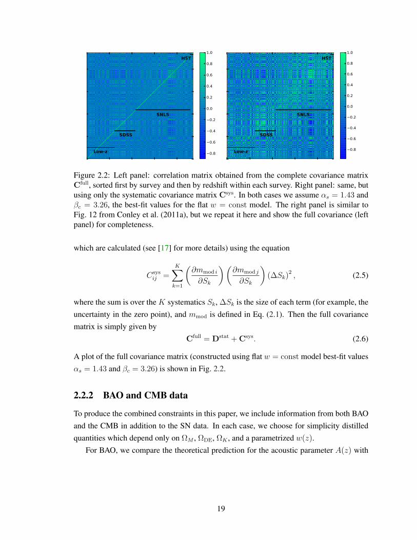
2.2 Left panel: correlation matrix obtained from the complete covariance matrixCfull, sorted first by survey and then by redshift within each survey. Rightpanel: same, but using only the systematic covariance matrix Csys. In bothcases we assume αs = 1.43 and βc = 3.26, the best-fit values for the flatw = const model. The right panel is similar to Fig. 12 from Conley et al.(2011a), but we repeat it here and show the full covariance (left panel) forcompleteness. . . . . . . . . . . . . . . . . . . . . . . . . . . . . . . . . . . . 19

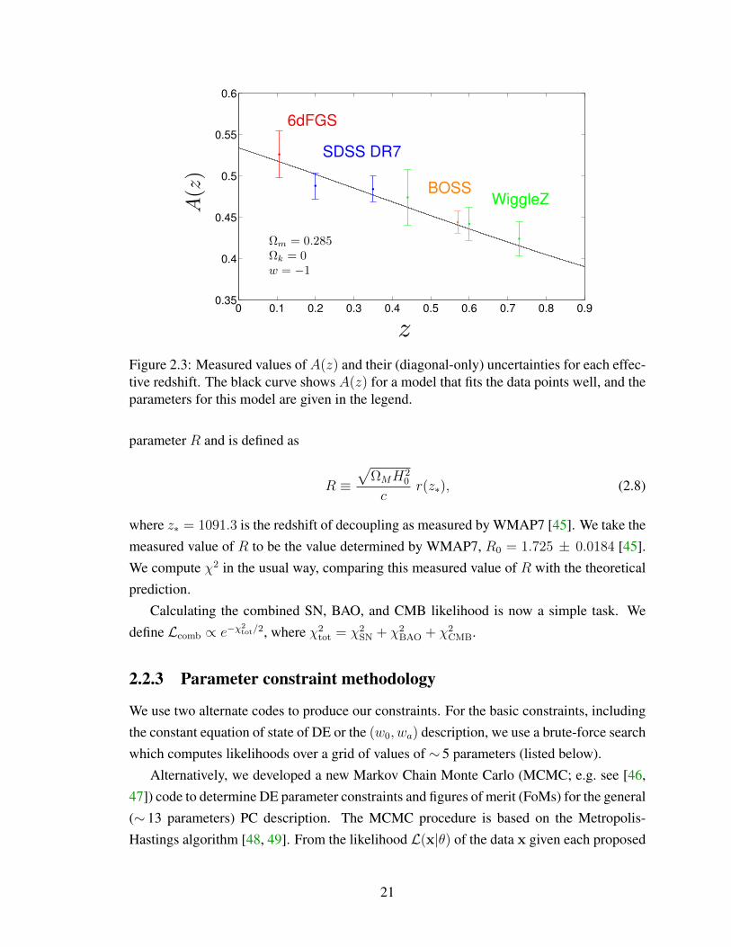
2.3 Measured values of A(z) and their (diagonal-only) uncertainties for each ef-fective redshift. The black curve shows A(z) for a model that fits the datapoints well, and the parameters for this model are given in the legend. . . . . . 21

2.4 68.3%, 95.4%, and 99.7% likelihood constraints on ΩM and w, assuming aconstant value for w and a flat universe. We use only SN data and marginalizeover the nuisance parameters. We compare the case of diagonal statisticalerrors only (shaded blue) with the full covariance matrix (red). . . . . . . . . . 24

2.5 68.3%, 95.4%, and 99.7% likelihood constraints on αs and βc, assuming aconstant value for w and a flat universe. We use only SN data and marginalizeoverM, ΩM , and w. We compare the case of diagonal statistical errors only(shaded blue) with the full covariance matrix (red). . . . . . . . . . . . . . . . 24

2.6 68.3%, 95.4%, and 99.7% likelihood constraints on w0 and wa in a flatuniverse, marginalized over ΩM and the nuisance parameters. The leftpanel shows SN-only constraints, while the right panel shows combinedSN+BAO+CMB constraints. The shaded blue contours represent constraintswith only statistical SN errors assumed (Dstat), while the red contours rep-resent the full SN covariance matrix (Cfull). Note that the ΛCDM model(w0, wa) = (−1, 0), represented by the black dashed lines, is fully consistentwith the data. . . . . . . . . . . . . . . . . . . . . . . . . . . . . . . . . . . . 25

viii

2.7 The first 10 PCs, e1(z)–e10(z), used in our analysis, in order of increasingvariance (bottom to top). The PCs were obtained assuming the observablequantities centered at the fiducial ΛCDM model, but with actual errors fromthe current data. See text for details. . . . . . . . . . . . . . . . . . . . . . . . 27

2.8 68.3%, 95.4%, and 99.7% likelihood constraints for all pairwise combinationsof the 13 cosmological parameters using the combined SN+BAO+CMB data.Diagonal boxes show the 1D marginalized likelihood for each parameter. Theblack contours illustrate the case of diagonal statistical SN errors only (Dstat),while the red contours (Cfull) also include the systematic SN covariance ma-trix. The parameter ordering is (top to bottom, or left to right): matter densityrelative to critical ΩM , the 10 PC amplitudes α1–α10, and the stretch and colornuisance parameters αs and βc. Note the good constraints on all parametersexcept for the last few PC amplitudes. . . . . . . . . . . . . . . . . . . . . . . 30

2.9 Marginalized SN+BAO+CMB constraints on the 10 PC amplitudes. Thedashed vertical lines represent the prior limits. Black curves represent con-straints from the diagonal statistical SN errors only, while the red curves cor-respond to the full SN covariance matrix. The black and red number in eachpanel shows the ratio of the PC error to the rms of the top-hat prior for thestatistical-covariance and full-covariance case, respectively. Note the goodconstraints on all PC amplitudes except for the last few. . . . . . . . . . . . . . 31

2.10 Top panel: FoM as a function of the number of PCs included, with the blackline showing the statistical-only FoM and the red line showing the FoM withsystematics included (See Eq. (2.16) for the definition of the FoM). Bottompanel: ratio of the FoM with systematic errors considered in the SN Ia data tothat with only statistical errors considered. BAO and CMB constraints wereincluded in both cases. Notice that the FoM ratio levels off after approximatelyfive PCs have been included. Note that here we have considered the first 15PCs (as opposed to 10 in Figs. 2.7-2.9) to show that the FoM indeed flattensoff as the PCs become very poorly constrained. . . . . . . . . . . . . . . . . . 32

2.11 Effects on the BAO-only (left panel) and BAO+CMB+SN (right panel) con-straints in the ΩM–w plane with (red) and without (shaded blue) the finitedetection significances of the BAO features taken into account. Note that thedifferences are modest in the BAO-only case and negligible in the combinedcase. . . . . . . . . . . . . . . . . . . . . . . . . . . . . . . . . . . . . . . . . 34

3.1 Likelihood curves for a constant equation of state w in a flat universe, usingPlanck CMB data (left panel) and WMAP9 CMB data (right panel). We com-pare constraints from CMB + BAO data alone (dashed black) to those whichadditionally include SN Ia data from SNLS3 (blue), Union2.1 (green), or PS1(dashed red). All likelihoods are marginalized over other cosmological andnuisance parameters, as explained in the text. . . . . . . . . . . . . . . . . . . 43

ix

3.2 Evolution of the mass step predicted from a toy model calibrated using datafrom the Nearby Supernova Factory. This is similar to Fig. 11 of Rigault etal. (2013), though we include a region of uncertainty by propagating errors inthe mass step and local star-forming fraction measured at z = 0.05 from theNearby Supernova Factory data. Vertical lines separate the three redshift bins,each of which contains twoM nuisance parameters, one for each host galaxymass range. . . . . . . . . . . . . . . . . . . . . . . . . . . . . . . . . . . . . 46

3.3 Effect of allowing for evolution of the mass step in redshift bins in the SNIa analysis. Left: 68.3%, 95.4% and 99.7% likelihood contours in the Ωm–w plane for SNLS3 data analyzed the standard way with two M nuisanceparameters (filled blue) and a new way with sixM parameters (open red), onefor each of two mass bins and three redshift bins. Planck + BAO constraints(open black) are overlaid for comparison. Right: 68.3% contours in the sameplane for combined Planck + BAO + SNLS3 data using one, two, or six Mparameters. . . . . . . . . . . . . . . . . . . . . . . . . . . . . . . . . . . . . 47

3.4 Residuals of SN Ia magnitudes, binned by redshift (inverse-covarianceweights), for SNLS3 (blue) and Union2.1 (red). All curves and data pointsare relative to a flat ΛCDM cosmology with Ωm = 0.3, which is roughly thebest-fit value from CMB and BAO data. The plot shows the degree to whichSNe in each redshift range pull toward w < −1, and we show several theorycurves with constant w for comparison. . . . . . . . . . . . . . . . . . . . . . 48

3.5 Effect of each individual SNLS3 SN on the combined constraint on the equa-tion of state, as a function of redshift (top left), host galaxy stellar mass (topright), stretch (bottom left), and color (bottom right). The blue points show theshift ∆w in the final constraint on w due to each individual SN. The red circlesshow the combined (summed) pull from each bin in the particular quantity. . . 50

3.6 Effect of an external H0 prior on the constant equation of state. We show theeffect on Planck + BAO constraints (black) and on combined Planck + BAO+ SN constraints separately for PS1 (red) and SNLS3 (blue), where the errorbars bound 68.3% and 95.4% of the likelihood for w. The external prior hasan uncertainty of 2.4 km/s/Mpc in each case, mimicking the uncertainty in theRiess et al. (2011) measurement. . . . . . . . . . . . . . . . . . . . . . . . . . 52

4.1 Number density of galaxies per steradian for our fiducial survey. Galaxies areassigned to the five redshift bins in proportion to the areas of the colouredregions, each spanning ∆z = 0.2. . . . . . . . . . . . . . . . . . . . . . . . . 62

4.2 Multiplicative effect due to our fiducial calibration errors with σ2c = 0.1 dis-

tributed on large scales ` ≤ 20. The biased power spectrum T` (black points)is compared to the true power spectrum C` (solid lines) for three of the fiveredshift bins of our fiducial survey. The spectra are binned in ` with inverse-variance weights, and the error boxes include cosmic variance and shot noise. . 63

4.3 Forecasted 68.3, 95.4, and 99.7 per cent joint constraints on the w0–wa darkenergy parametrization for our fiducial survey, using information from ` = 21through `max = 2,000 without calibration errors (blue) and with multiplicativecalibration errors from ` ≤ 20 with σ2

c = 0.1 (red). . . . . . . . . . . . . . . . 65

x

4.4 Shift in parameter-space χ2 due to multiplicative calibration errors as a func-tion of the maximum multipole used in the analysis. We show the effecton the full five-dimensional space of parameters (black) along with the two-dimensional spaces of Ωm and w with fixed wa = 0 (blue) and w0 and wa(red). The overlaid dashed grey lines mark the 68.3, 95.4, and 99.7 per centbounds for a two-dimensional Gaussian distribution (for comparison with thered or blue lines). . . . . . . . . . . . . . . . . . . . . . . . . . . . . . . . . . 66

4.5 Shift in the full five-dimensional parameter-space χ2 due to multiplicative cal-ibration errors as a function of the maximum multipole used in the analysis,for calibration-error parameters measured up to various `max, meas. The over-laid dashed grey lines mark the 68.3, 95.4, and 99.7 per cent bounds for afive-dimensional Gaussian distribution. . . . . . . . . . . . . . . . . . . . . . 67

4.6 Statistical error (blue) and bias (dashed red) on w0 (left) and wa (right) as afunction of the maximum multipole `max, meas at which calibration errors aremeasured. . . . . . . . . . . . . . . . . . . . . . . . . . . . . . . . . . . . . . 68

5.1 Fits to an isotropic-only version of the BAO data (black points), where weuse the direct isotropic measurement from BOSS CMASS (z = 0.57) andan isotropic measurement derived from the LyαF anisotropic measurements(z = 2.34). We show the best fit to this modified BAO set for ΛCDM with Ωm

and rd varied (solid black), power law cosmology with n and rd varied (solidblue), and power law cosmology with n = 1.5 and only rd varied (dashed red),where the value n = 1.5 is roughly the value required to fit the SN Ia data. . . . 83

5.2 Hubble diagram for the JLA SN compilation, where the measured distancemoduli have been standardized separately for ΛCDM (blue points) and theRh = ct cosmology (red points). The best-fit (Ωm = 0.29) ΛCDM model(solid blue) is plotted along with theRh = ctmodel (dashed red). We show theSN data without (left panel) and with (right panel) systematic errors included.The distance moduli are binned in redshift with inverse-covariance weights. . . 86

6.1 Comparison of the signal (left panel) and noise (right panel) contributions tothe full covariance matrix for the 111 SNe at z < 0.05 from the JLA compilation. 99

6.2 Constraints on the parameter A that quantifies the amount of velocity corre-lations (A = 1 is the standard ΛCDM value). The JLA data are consistentwith A = 1 but do not rule out the noise-only hypothesis A = 0. JLA andUnion2 give somewhat different constraints, though they are not statisticallyinconsistent. Note that differences remain even after restricting to the ratherlarge subset of SNe that they have in common (dashed lines). . . . . . . . . . . 101

6.3 A slice through the 3D likelihood for excess bulk velocity. The direction isfixed to be nmax-like (different for each dataset), while the amplitude of thedipole is varied and allowed to be positive or negative. Conclusions about thebulk flow would differ significantly if the velocity signal covariance were setto zero (dashed lines), as in most previous work on the subject. . . . . . . . . 103

xi

6.4 Angle-averaged posterior on the amplitude of bulk velocity in excess of thecorrelations captured by the full ΛCDM velocity covariance. Both JLA andUnion2 data are consistent with zero velocity, with relatively large error. Theconclusion would again be very different if the velocity covariance were arti-ficially set to zero (dashed lines). . . . . . . . . . . . . . . . . . . . . . . . . . 104

xii

LIST OF TABLES

Table1.1 Summary of results for simple one-component universes. . . . . . . . . . . . . 6

2.1 Summary of SN Ia observations included in this analysis, showing the numberof SNe included from each survey and the approximate redshift ranges. . . . . 17

2.2 Summary of measurements of distilled BAO parameter A(z). We show thesurvey from which the measurement comes, the effective redshift of the survey(or its subsample), and the measured value A0. . . . . . . . . . . . . . . . . . 20

2.3 Values of the FoM (Eq. (2.12)) for SN alone (middle row) and SN+BAO+CMB(bottom row). The middle column shows the FoMs for the statistical covari-ance matrix Dstat only, while the right column shows the FoMs for the fullcovariance matrix Cfull. Note that including the systematics reduces the FoMby a factor of two to three. . . . . . . . . . . . . . . . . . . . . . . . . . . . . 26

3.1 Summary of BAO measurements combined in the analysis. We list the surveyfrom which the measurement comes, the effective redshift of the survey, theobservable parameter constrained, and its measured value. . . . . . . . . . . . 43

3.2 Mean values and standard deviations of the CMB measurements used in ouranalysis. The measurements for both Planck and WMAP9 were obtained usingthe Markov chains provided by the Planck collaboration. We assumed themodel with a flat universe and constant dark energy equation of state, the samemodel we constrain in this analysis. . . . . . . . . . . . . . . . . . . . . . . . 45

5.1 Summary of BAO measurements combined in this analysis. We list the samplefrom which the measurement comes, the effective redshift of the sample, theobservable quantity constrained, and its measured value. The anisotropic mea-surements from BOSS CMASS are correlated with coefficient −0.52, whilethose from BOSS LyαF are correlated with coefficient −0.48. Otherwise, weassume the measurements to be statistically independent. . . . . . . . . . . . . 77

5.2 Best-fit values of each parameter varied for each model and data combination. . 815.3 Results of the model comparison. For each of the models and data combina-

tions, we list the number of parameters k that were varied, the total number ofdata points N , the best-fit χ2

min, the probability P (χ2min, ν) that a greater χ2

mincould occur due to chance alone for degrees of freedom ν = N − k, and thelikelihood of the model relative to ΛCDM for the AICc, BIC, and Bayes factormodel comparison statistics. . . . . . . . . . . . . . . . . . . . . . . . . . . . 82

xiii

6.1 Summary of numerical results. For both JLA and Union2, we show the best-fit, maximum-likelihood (ML) values and 95% confidence intervals for A. Wealso show the quantity ∆χ2 (that is, −2∆ lnL) between the best-fit value andspecial values A = 0 (no velocity signal) and A = 1 (ΛCDM velocity signal).We also show ML and 95% intervals for bulk velocity in the best-fit directionand 95% intervals for angle-averaged bulk velocity (here we do not report MLvalues, which are near zero). All velocities are in units of km/s. . . . . . . . . 107

xiv

LIST OF APPENDICES

A Analytic Marginalization Over Multiple SN Ia Absolute Magnitudes . . . . . 113

B The Biased Angular Power Spectrum . . . . . . . . . . . . . . . . . . . . . . . 116

xv

CHAPTER 1

Introduction

1.1 Modern Cosmology from the Cosmological Principle

Cosmology is the subfield of astrophysics concerned with the properties of the universe as awhole, and it has ancient roots. For thousands of years, cultures throughout the world havesought to understand and explain the universe in the context of their world view. Througha mixture of creation stories and other philosophies, often inspired by and tied to carefulobservations of the night sky, people have tried to answer the big questions: Where did wecome from? What else is out there? How does it all work? Descriptions of the universewere as numerous and diverse as the cultures that created them.

On the other hand, only very recently has cosmology become an established science.The existence of distant galaxies was not accepted by the scientific community until theearly-to-mid 20th century. Even after our basic cosmological picture was established, mea-surements were so uncertain that determinations of certain key parameters, such as theHubble expansion constant and the age of the universe, varied by factors of two. Only inthe last decade or two have we been able to turn cosmology into a precise science; however,the result is that we are now able to determine many of these important parameters withpercent-level measurement uncertainties.

Cosmology can be modeled in a surprisingly simple framework. On small scales, theheterogeneity of the universe is apparent. In our Solar System, dense planets and asteroidsmove along stable orbits, leaving a near vacuum everywhere else. On galactic scales, wefind dense galaxies and galaxy clusters in some regions and voids elsewhere. On even largerscales, however, we can map the enormous filaments of large-scale structure that carry us tothe edge of the observable universe. On these scales (&100 Mpc), we can often rely on the(testable) assumptions of homogeneity and isotropy. Homogeneity is the statement that theuniverse is the same everywhere, while isotropy is the statement that there is no preferreddirection. They are consequences of the cosmological principle, which asserts that on the

1

largest scales, all properties of the universe are the same for all observers.From these conditions, we can write down a compatible spacetime metric in the frame-

work of general relativity (see e.g. [6]). We choose one which allows the spatial coordinatesto scale (equally) with time and which allows for space to have uniform intrinsic curvature,which can be realized in one of three ways, as dictated by the value of the constant k. Thepossibilities for k are positive curvature (spherical geometry, closed universe), zero cur-vature (flat geometry, critical universe), or negative curvature (hyperbolic geometry, openuniverse). One can show that the appropriate metric is

ds2 = −dt2 + a(t)2

[1

1− kr2dr2 + r2

(dθ2 + sin2 θ dφ2

)], (1.1)

where we have set the speed of light c = 1. This is the famous Friedmann-Lemaıtre–Robertson-Walker (FLRW) metric. From this interval, one can immediately deduce thecorresponding metric tensor gµν and compute the Christoffel symbols, the Riemann tensor,the Ricci tensor Rµν , and the Ricci scalar R. The resulting Einstein tensor is given by

Gµν = Rµν −1

2gµνR

= diag[

3 (k + a2)

a2, − Z

1− kr2, −r2 Z , −r2 sin2 θ Z

], (1.2)

where Z ≡ 2aa+a2+k. For consistency, we should apply the assumptions of homogeneityand isotropy to the stress-energy tensor. With the assumption of a perfect fluid — one withno shear stresses, heat conduction, or viscosity, the stress-energy tensor is simply

Tµν = (ρ+ p)UµUν + p gµν = diag[ρ ,

p a2

1− kr2, p a2r2 , p a2r2 sin2 θ

], (1.3)

where ρ is the fluid’s energy density, p is its pressure, and Uµ = (1, 0, 0, 0) is the four-velocity. We can now solve the Einstein field equations Gµν = 8πG Tµν using the above.The equation for the 00 component immediately produces the following result:(

a

a

)2

=8πG

3ρ− k

a2. (1.4)

2

The tensor trace gives a second independent result:

gνµ Gµν = 8πG gνµ Tµν

−R = 8πG T νν

− 6

a2

(aa+ a2 + k

)= 8πG (−ρ+ 3p) (1.5)

a

a= −4πG

3(ρ+ 3p) . (1.6)

Eq. (1.6) follows from using Eq. (1.4) to rewrite Eq. (1.5). There are, in general, 10 inde-pendent field equations to solve, but our assumptions (symmetries) leave only four nontriv-ial equations, two of which are redundant. Although there are no more independent results,it is possible and often useful to combine the above two equations and write down a third.If we multiply Eq. (1.4) by a2, take its time derivative, and substitute for a/a in Eq. (1.6),we obtain:

ρ = −3a

a(ρ+ p) . (1.7)

Often these equations are collectively referred to as the Friedmann equations, but Eq. (1.4)is often called the Friedmann equation, with Eq. (1.6) called the acceleration equation andEq. (1.7) called the fluid equation, an expression of conservation of energy. The quantitya is the scale factor, and it is the (time-dependent) factor that translates between comovingdistance and physical distance, where comoving distance (also called coordinate distance)is unchanged by any expansion or contraction of the universe. Comoving distance coincideswith physical distance at the value a = 1.

1.2 The Cosmological Constant and Simple Cosmologies

Einstein, motivated by his expectation of a steady-state universe, added a term Λ gµν to theEinstein tensor, where Λ is called the cosmological constant. Today, it is widely acceptedthat the universe is expanding and not in a steady state; however, the possibility of a cos-mological constant is intriguing. In fact, if one simply writes the constant term on the otherside of the equation, Gµν = 8πG Tµν − Λ gµν , it has the appearance of a vacuum energy

density, since it contributes to the stress-energy tensor Tµν . With the cosmological constantincluded, Eq. (1.4) becomes (

a

a

)2

=8πG

3ρ− k

a2+

Λ

3, (1.8)

3

while Eq. (1.7) is unchanged.To understand the effect of a so-called vacuum energy, we will first study the Friedmann

equations in more detail. Let us rewrite Eq. (1.8) in a more useful form. The important thingto remember is that ρ represents the total energy density of the homogeneous universe. Butthe universe does not contain only one type of fluid. It contains both matter (ordinarybaryonic matter and non-baryonic cold dark matter) and radiation (hot, relativistic matterparticles like light neutrinos would also be included here). It is also convenient to describeboth curvature and the cosmological constant in terms of an energy density, though it isimportant to emphasize that curvature does not actually contribute to a physical energydensity, unlike Λ, which might. So let us define ρi to be the energy density of species ionly, and then let us also define

ρk =3

8πG

k

a2, ρΛ =

Λ

8πG, (1.9)

so that the Friedmann equation becomes

H2 =8πG

3(ρ− ρk) , ρ = ρm + ρr + ρΛ , H ≡ a

a. (1.10)

Here, H is the Hubble parameter, which describes the rate of expansion of the universe;like a, it is a function of time.

One further simplification is helpful. Notice that if we set ρ = 3H2/(8πG) inEq. (1.10), it would imply that k = 0 and the universe is flat. Since k is a constant, ifthis is the case at one time, then k is always zero and it is thus impossible for an expandinguniverse (a > 0) to contract, though the rate of expansion will approach zero as t → ∞.This motivates the definition of the critical density ρcrit = 3H2/(8πG) and the fractionaldensity Ωi = ρi/ρcrit. The Friedmann equation simply becomes Ω− Ωk = 1.

To proceed further, we observe that the two independent Friedmann equations involvethree variables (a, ρ, and p). In order to get some real solutions, we must close the system byrelating two of these quantities. The most obvious way to do that is by assuming an equationof state, which is a relationship between p and ρ. For the perfect fluids that we want todescribe, the equation of state has the form pi = wiρi, where wi is a constant. For matter,which is assumed to be cold (non-relativistic), the pressure is negligible compared to theenergy density, so we set wm = 0 so that pm = 0. For radiation, we know from statisticalmechanics that pr = ρr/3 so that wr = 1/3. Although not the case for the other fluids,we expect the vacuum stress-energy tensor to be Lorentz invariant (all observers should seethe same vacuum). Since Tµν ∝ gµν when pΛ = −ρΛ, we have wΛ = −1. For curvature,

4

we can deduce the effective wk from the fluid equation. Substituting the definition of ρk inEq. (1.9) into Eq. (1.7) and specifying pk = wkρk, we find that wk = −1/3.

We expect the fluid equation to be valid for any species i. Since we now know thepressure as a function of energy density for each species, we can solve Eq. (1.7) to find theenergy density ρi as a function of the scale factor a:

ρi = ρi,0 a−3(1+wi). (1.11)

It is customary to denote present values with a subscript 0 and to fix a0 = 1 (since a is justa scale factor, its overall normalization has no physical significance, and this is the mostconvenient choice).

This result is easy to understand. For matter, wm = 0, so ρm ∝ a−3. This is whatwe expect: given some fixed amount of matter, its average mass density is inversely pro-portional to its volume. The mass of non-relativistic matter is proportional to its energy,and the actual volume of the universe is proportional to a3, so this result is consistent withexpectations. For radiation (wr = 1/3), we find that ρr ∝ a−4. Here, we still expect thesame dilution factor that applies to matter, but there is an extra factor of 1/a. This is dueto the fact that, as the universe expands, so do the wavelengths of photons, and the energyof a photon E = hc/λ is inversely proportional to its wavelength. For the cosmologicalconstant (wΛ = −1), we find ρΛ to be constant. This may seem surprising, but if Λ is in-terpreted as vacuum energy, this makes sense: the volume of the universe may change, butthe amount of vacuum energy is proportional to the volume of the vacuum, so the densityis constant. The curvature result (ρk ∝ a−2) is less intuitive but is a consequence of theway we defined curvature density.

Finally, we can rewrite the Friedmann equation one more time by inserting the expres-sions for ρi(a) and making use of the parameters Ωi that we defined earlier:

H2(a) = H20

[Ωma

−3 + Ωra−4 + ΩΛ − Ωka

−2], (1.12)

where these Ωi refer to present values even though the subscript 0 is almost always omitted.Defining the cosmological redshift of photons as

1 + z ≡ λobs

λemit=

1

a, (1.13)

we can express Eq. (1.12) equivalently in terms of the redshift:

H2(z) = H20

[Ωm (1 + z)3 + Ωr (1 + z)4 + ΩΛ − Ωk (1 + z)2

]. (1.14)

5

Equations (1.12) and (1.14) are probably the most illuminating and most useful forms ofthe Friedmann equation.

Solving for a(t), for instance, is now straightforward, though for a realistic universethe Friedmann equation must be integrated numerically for a given choice of the Ωi andH0 parameters. To gain insight, we can solve Eq. (1.12) assuming that the energy densityof the universe is dominated by one of the fluids so that we can ignore the others. Thismay seem like a terrible oversimplification, since we know that the universe has multiplecomponents and has had multiple components in the past; however, since each fluid tendsto dominate during a different epoch, these simpler solutions could in principle be stitchedtogether to obtain a more complete picture. So let us now find the solution for a(t) when afluid with equation of state parameter w is dominant. By integrating the simplified versionof Eq. (1.12),

H2 = H20 a−3(1+w), (1.15)

we find

a(t) =

(t

t0

) 23(1+w)

, w 6= −1. (1.16)

Here we have assumed that the universe had zero size (a = 0) at a time t = 0 (correspond-ing to the Big Bang) and used the present as a reference point (a(t0) = 1). For the specialcase w = −1, one can go back to Eq. (1.15). The result is

a(t) = eH0(t−t0) = e√

Λ/3 (t−t0), w = −1. (1.17)

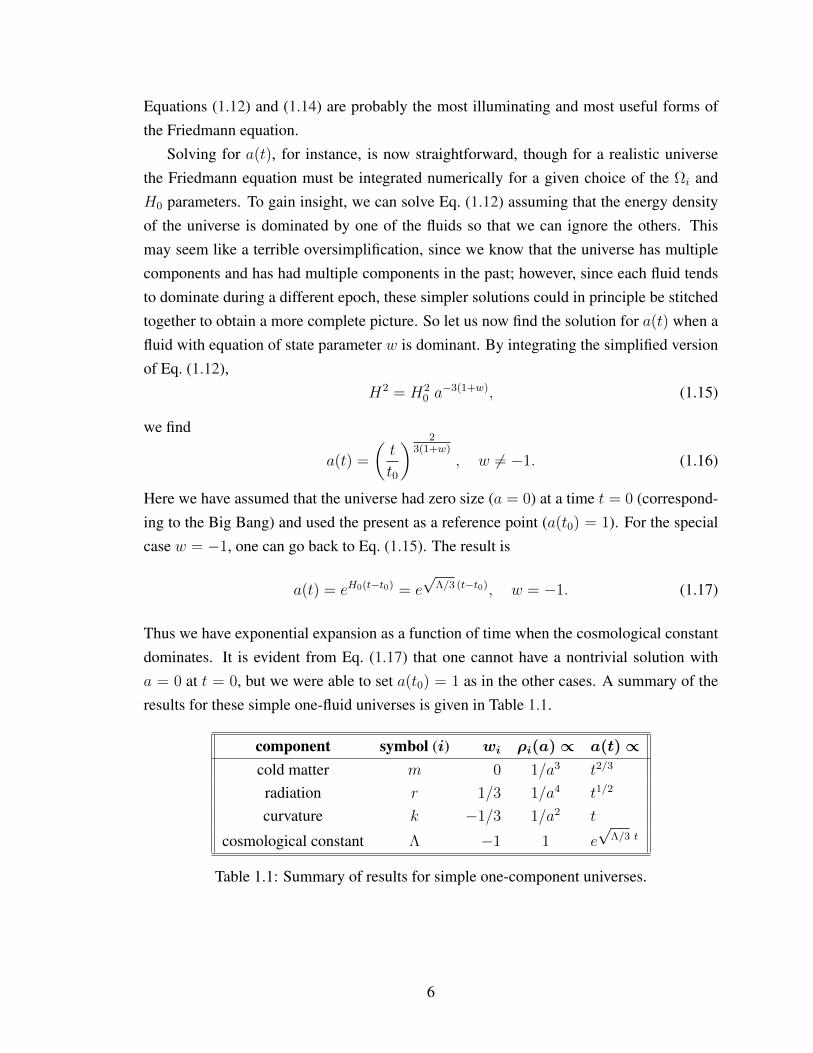
Thus we have exponential expansion as a function of time when the cosmological constantdominates. It is evident from Eq. (1.17) that one cannot have a nontrivial solution witha = 0 at t = 0, but we were able to set a(t0) = 1 as in the other cases. A summary of theresults for these simple one-fluid universes is given in Table 1.1.

component symbol (i) wi ρi(a) ∝ a(t) ∝cold matter m 0 1/a3 t2/3

radiation r 1/3 1/a4 t1/2

curvature k −1/3 1/a2 t

cosmological constant Λ −1 1 e√

Λ/3 t

Table 1.1: Summary of results for simple one-component universes.

6

1.3 The Standard Cosmological Model

The currently favored cosmological model features a universe that consists mostly of colddark matter and dark energy in the form of a cosmological constant. A Big Bang occurred13.8 billion years ago, with space itself expanding from a very small, hot, and dense ini-tial state. Roughly 10−36 seconds after the Big Bang, inflation — a period of very rapidexpansion — occurred, driving any intrinsic curvature to very near zero and seeding theuniverse with small, Gaussian density perturbations. A few seconds later, protons and neu-trons fused to form hydrogen and helium along with trace amounts of heavier elements in aprocess called Big Bang nucleosynthesis (BBN), which lasted several minutes. After about380,000 years, at a redshift z ' 1100, the universe cooled enough for electrons and protonsto combine and form neutral hydrogen, allowing photons to free stream. These photons areobserved today at a temperature of 2.73 K as the cosmic microwave background (CMB).The universe then entered a period, the Dark Ages, which lasted until the epoch of reion-ization when the first stars formed and partially reionized the universe. The formation ofgalaxies and galaxy clusters followed, creating a large-scale structure imprinted with theprimordial density perturbations and acoustic waves. At z ∼ 1, roughly half the presentage, the expansion of the universe began to accelerate due to the cosmological constant Λ,which now dominates the energy budget.

This model is called ΛCDM, since the primary ingredients are a cosmological constantand cold dark matter. With only six free parameters, ΛCDM accurately describes an enor-mous breadth of cosmological observations and has passed stringent tests in recent years.The six parameters are: the physical densities of cold dark matter and baryons Ωch

2 andΩbh

2, the Hubble constant H0 = 100h km/s/Mpc, the amplitude and index of a power lawprimordial power spectrum P (k) = As (k/kpiv)

ns , and the optical depth at reionization τ .With the minor exception of τ , which is rather poorly constrained at present, Planck CMBobservations [7] alone measure all of these parameters with roughly 1% precision.

Testing the ΛCDM model and characterizing the nature of dark energy are among thecentral challenges for modern cosmology. Given the robustness of ΛCDM, it is not surpris-ing that most alternative models are extensions in the sense that ΛCDM is embedded as aspecial case. Such extensions include a non-minimal neutrino sector, where the neutrinomass sum or the effective number of species is allowed to vary; a non-minimal dark energysector, where the equation of state is allowed to be different from −1 and vary with cosmictime; a nonzero value for intrinsic curvature; and a non-minimal inflationary epoch thatmanifests running of the spectral index or a nonzero tensor-to-scalar ratio. Many of theseone- or two-parameter extensions are already well-constrained by combined data (e.g. [7]).

7

1.4 Distance Probes of Dark Energy

Here we give a brief overview of the three classic distance probes of dark energy andcosmic expansion: Type Ia supernovae (SNe Ia), CMB fluctuations, and baryon acousticoscillations (BAO).

1.4.1 SNe Ia

SNe Ia alone were used to discover dark energy [8, 9]. They function as bright standard can-dles — objects with roughly constant or otherwise deterministic luminosity whose apparentbrightnesses can be used to infer distance. SNe Ia are characterized spectroscopically bythe lack of a hydrogen line, distinguishing them from Type II SNe, and the presence of asingly ionized silicon line, distinguishing them from Type Ib/c SNe. While the other typesare associated with the core collapse of a dying massive star, it is thought that a SN Iaoccurs when mass is accreted onto the surface of a white dwarf from a companion star.When the white dwarf accumulates enough mass to exceed the Chandrasekhar limit, thewhole star detonates, releasing an enormous amount of energy in the process. Given thisspecific mass limit (∼ 1.4M) for white dwarves, it is not surprising that all SNe Ia releaseapproximately the same amount of energy.

It is important to note that, whether or not our understanding of this mechanism iscorrect, it is an empirical fact that there exist stellar explosions, distinguishable from otherstellar explosions, that tend to have similar peak luminosities. Since these explosions arevery bright, they can be observed at high redshifts, making them useful for measuringcosmological distances.

The apparent magnitude of a SN Ia is given by

m(z) = 5 log10

[H0

cdL(z)

]+M , (1.18)

where dL is the luminosity distance andM is an offset that depends on the Hubble constantH0 and the absolute magnitude of a SN Ia, which is a priori unknown. The luminosity

8

distance is given by dL(z) = (1 + z) r(z), where

r(z) ≡

R0 sin [χ(z)/R0] Ωk > 0

χ(z) Ωk = 0

R0 sinh [χ(z)/R0] Ωk < 0

(1.19)

χ(z) ≡∫ z

0

c

H(z′)dz′ , R0 ≡

c

H0

1√|Ωk|

. (1.20)

For a flat universe, the Hubble parameter has the form

H(z) = H0

√Ωm (1 + z)3 + ΩX (1 + z)3(1+w) , (1.21)

where we have left out the radiation contribution, which is negligible for the relativelylow redshifts (z . 2) where we find SNe. Also, we have replaced the Λ term with amore general dark energy term, assuming a constant equation of state that reduces to Λ ifw = −1.

SNe are not perfect standard candles; their absolute magnitudes vary with a scatter of∼0.3 mag, corresponding to a distance error of ∼14%. But useful empirical correlationsexist between the peak apparent magnitude and other light-curve properties, notably thelight curve’s stretch (i.e. broadness, decline time) and color measure (e.g. magnitude dif-ference between two bands). As a rule of thumb, broader is brighter, and bluer is brighter.These relations further standardize SNe Ia, reducing the intrinsic scatter to ∼0.15 mag orless for a distance error of less than 7%.

Since these standardization relations are empirical, substantial current work is focusedon how best to model them, determining whether other useful correlations exist, and at-tempting to quantify any possible evolutionary effects.

1.4.2 CMB

The CMB contains a wealth of cosmological information; it can separately inform us aboutthe densities of dark matter and baryons, the physics of inflation, and the geometry of theuniverse [7]. Until relatively recently, most of this information came from measurementsof the power spectrum of temperature fluctuations, but today these are joined by measure-ments of the E-mode and B-mode polarization spectra as well as the CMB lensing potential.

On the other hand, CMB observations are very limited in their ability to constrain gen-eral models of the dark energy equation of state. Since dark energy was negligible at highredshifts, the CMB is only sensitive to dark energy in how it affects the CMB photons on

9

their way to us. While this includes some information from the effect of dark energy ongrowth of structure, via the integrated Sachs-Wolfe (ISW) effect and gravitational lensing,most of the information is encapsulated by a single measure of distance to the surface ofrecombination. Since the redshift z∗ of recombination is not known a priori, it is mostappropriate to summarize CMB distance information with a set of observables. A commonchoice is to measure z∗ along with

la ≡ π (1 + z∗)dA(z∗)

rs(z∗), (1.22)

R ≡√

ΩmH20

c(1 + z∗) dA(z∗) , (1.23)

where la is the acoustic angular scale, R is the so-called shift parameter, and rs is the soundhorizon — the distance that a sound wave travels in a time t since the Big Bang, given by

rs(t) =

∫ t

0

csadt′ , cs =

c√3 (1 +R)

, (1.24)

where the sound speed cs depends on the ratio of baryon energy density to photon energydensity, with R ≡ 3ρb/(4ργ).

Although these observables basically provide one distance measurement, it is a veryprecise distance to a very high redshift, so the approximate result is that it effectively fixesone parameter describing the geometry of the late universe, for instance, a constraint onΩm or a narrow constraint band in the Ωm – w plane.

It is important to be aware of any possible model dependence of these observables.While they are typically independent of any dark energy model, they will be sensitive tothe overall cosmological model. For instance, the measured value of z∗ might shift if non-standard neutrino physics is assumed.

1.4.3 BAO

BAO are the regular, periodic fluctuations of visible matter density in large-scale structure(LSS) resulting from sound waves propagating in the early universe. The BAO signal cor-responds to a peak in the correlation function at a comoving scale of∼150 Mpc. This scaleis an excellent standard ruler, and measuring the location of the peak at various redshiftswill probe expansion and dark energy. The first detection of the feature in the SDSS LRGsample [10] has since been replaced by several more precise measurements, including oneat z = 0.106 (6dF, [11]), z = 0.32 (BOSS LOWZ, [12]), and z = 0.57 (BOSS CMASS,[13]), with the latter achieving a ∼1% distance measurement. BAO can also be detected in

10

other LSS tracers, such as Lyman-α forests, where the feature has been detected at z = 2.34

using BOSS quasars (e.g. [14]).The typical observable derived from the BAO measurement is DV (zeff)/rd, where zeff

is the median redshift of the LSS survey, rd ≡ rs(zd) is the size of the sound horizon at theepoch of baryon drag, and DV is a spherical-volume-averaged distance defined by

DV (z) ≡[(1 + z)2 d2

A(z)cz

H(z)

]1/3

. (1.25)

Recently, it has been possible to achieve high signal-to-noise detections using the trans-verse and radial correlation functions separately, resulting in separate measurements of(1 + zeff) dA(zeff)/rd and czeff/H(zeff)/rd. In addition to providing more cosmological con-straining power, these anisotropic measurements can be used to look for exotic departuresfrom the standard model.

One important caveat when using the BAO observables is that the measurements areoften correlated. This is the case for the anisotropic measurements as well as for mea-surements at different redshifts and/or from different surveys if there is overlap in surveyvolume. Neglecting any significant correlation will lead to incorrect constraints and under-estimates of errors.

Also, note that comparing data to theory here requires a way to estimate the size of thesound horizon, which ultimately requires some information from the CMB, such as a prioron the sound horizon itself, priors on Ωmh

2 and Ωbh2, or some combination thereof. One

way around this is to use multiple BAO measurements as relative distance indicators, asone typically does with SNe Ia, and just marginalize over the sound horizon.

BAO measurements are generally thought to be robust and free of systematic effectsat least down to the 1% level, making them effective probes of dark energy, especially athigher redshifts, where they will likely out-perform SN Ia distances.

Fig. 1.1 illustrates how the three probes (SN Ia, CMB, BAO) complement one anotherto constrain dark energy by breaking degeneracies in parameter space. Combining theseand other probes not only allows us to more precisely determine cosmological parame-ters, it also provides a way to check for consistency and determine whether there are anyunaccounted-for systematic effects.

1.5 Outline

This goal of this dissertation is to investigate systematic effects and perform new cosmo-logical tests with observational probes of dark energy in anticipation of the precision dark

11

Figure 1.1: SN Ia, CMB, and BAO constraints on Ωm and ΩΛ in an open ΛCDM universe(left panel) and on Ωm and w in a flat universe where the dark energy equation of state isallowed to vary (right panel).

energy constraints expected in the near future.Chapters 2–4 study systematic effects in dark energy probes, focusing especially on

constraints from distance probes like SNe Ia. In Chapter 2, we quantify the effect of currentSN Ia systematic errors on dark energy constraints, both for simple parametrizations of theequation of state and for a general description with principal components. We consider bothSN-only and combined constraints and find that the SN Ia systematics typically degradefigures of merit by roughly a factor of three, illustrating their importance even for currentdata. Separately, we consider the effect on constraints of the finite detection significance ofthe BAO feature.

Chapter 3 investigates recent evidence for a phantom dark energy equation of stateusing three separate SN Ia compilations (SNLS3, Union2.1, and PS1) in combination withCMB distance information from either WMAP9 or Planck. Using this distance informationalone, we find nearly 2σ evidence for w < −1 when SNLS3 or PS1 is combined withPlanck. In the process, we introduce new tests to investigate systematic effects. We studythe dependence of the constraints on the redshift, stretch, color, and host galaxy stellarmass of SNe, but we find no unusual trends. In contrast, the constraints strongly dependon any external H0 prior: a higher adopted value for the direct measurement of the Hubbleconstant (H0 & 71 km/s/Mpc) leads to & 2σ evidence for phantom dark energy. GivenPlanck data, and assuming that ΛCDM is correct, we conclude that either the SNLS3 andPS1 data have systematics that remain unaccounted for or that the Hubble constant is belowabout 71 km/s/Mpc.

Chapter 4 is concerned with photometric calibration errors in the galaxy power spec-trum. We first point out the danger posed by the multiplicative effect of calibration errors,

12

where large-angle error propagates to small scales and may be significant even if the large-scale information is cleaned or not used in the cosmological analysis. We then propose amethod to measure the arbitrary large-scale calibration errors and use these measurementsto correct the small-scale (high-multipole) power which is most useful for constraining themajority of cosmological parameters. Using a Fisher matrix formalism, we demonstratethe effectiveness of our approach on synthetic examples and briefly discuss how it may beapplied to real data.

Chapters 5–6 focus on tests of the standard ΛCDM model. In Chapter 5, we usegoodness-of-fit and Bayesian model comparison techniques with model-independent SNIa and BAO data to test power law expansion as an alternative cosmological model. Wefind that neither power law expansion nor ΛCDM is strongly preferred over the other whenthe SN Ia and BAO data are analyzed separately but that power law expansion is stronglydisfavored by the combination. We treat the so-called Rh = ct cosmology (a constant rateof expansion) separately and find that it is conclusively disfavored by all combinations ofdata that include SN Ia observations and a poor overall fit when systematic errors in the SNIa measurements are ignored, despite a recent claim to the contrary. We discuss this claimand some concerns regarding hidden model dependence in the SN Ia data.

In Chapter 6, we use low-redshift SN Ia data to test for the presence of the peculiarvelocity correlations predicted for the standard ΛCDM model. We find no evidence for thepresence of these correlations, although, given the significant noise, the data is also consis-tent with them. We then consider the dipolar component of the velocity correlations — thefrequently studied “bulk velocity” — and explicitly demonstrate that including the velocitycorrelations in the data covariance matrix is crucial for drawing correct and unambiguousconclusions about the bulk flow. In particular, current SN data is consistent with no excessbulk flow on top of what is expected for ΛCDM and effectively captured by the covariance.We further clarify the nature of the apparent bulk flow that is inferred when the velocitycovariance is ignored.

13

CHAPTER 2

Dark Energy with SN Ia Systematic Errors

2.1 Introduction

Since the discovery of the accelerating universe in the late 1990s [8, 9], a tremendousamount of effort has been devoted to improving measurements of dark energy (DE) pa-rameters. As constraints on these parameters improved, controlling the systematic errorsin measurements became critical for continued progress. The systematics come in manyflavors, including a multitude of instrumental effects and astrophysical effects.

Type Ia supernovae (SNe Ia) were used to discover DE and still provide the best con-straints on DE. The advantage of SNe Ia relative to other cosmological probes is that ev-

ery SN provides a distance measurement and therefore some information about DE. Morerecently, SN Ia observations have been joined by measurements of baryon acoustic oscil-lations (BAO), which provide exceedingly accurate measurements of the angular diameterdistance in redshift bins. Cosmic microwave background (CMB) anisotropies come mostlyfrom high redshift and are thus not particularly effective in probing DE, but they do provideone measurement of the angular diameter distance to redshift z ' 1100 very accurately.Galaxy clusters also constrain DE usefully, while weak gravitational lensing is expected tobecome one of the most effective probes of DE in the near future. For recent comprehensivereviews of DE probes, see [15, 16].

In this work, we are interested in studying the effect of SN Ia systematics on DE con-straints by including the covariance of measurements between different SNe. The covari-ance includes primarily systematic errors, and for the first time it has been quantified indepth by [17]. Including the effects of the systematic errors, represented by nonzero co-variance, weakens the overall constraints on model parameters. Here we wish to explorethe effect of systematic errors for general models of DE described by a number of principalcomponents (PCs) of the equation of state, though we first consider these effects for sim-pler, more commonly used descriptions of the DE sector. We choose to combine the SN

14

Ia data with BAO and CMB measurements and estimate the effects of current systematicerrors in SN Ia observations. We then proceed to study another systematic concern that isparticularly relevant for BAO: whether the finite significance of the detection of the BAOfeature in various surveys, when taken into account, weakens the constraints imposed onDE parameters.

While we closely follow the accounting for the SN Ia systematics from [17], we notethat several other analyses have considered the effect of SN systematics. However, mostof these analyses only studied the effects of the systematic errors on the constant equationof state (e.g. [17–20]) or included the additional parameter wa to describe the variation ofthe equation of state with time (e.g. [21]). Notable exceptions are studies by [22] and [23],which considered a number of specific DE models with non-standard behavior, and [24]and [25], which parametrized the DE density in several redshift bins. Here our goal is to gobeyond any specific models and study the effects of systematic errors in current data on DEconstraints in the greatest generality possible. While a truly model-independent descriptionof the DE sector is of course impossible, a description of the expansion history in terms of10 or so parameters – which we adopt in this paper – comes close1. In this sense, ourpaper complements the recent investigations by [26, 27] (see also [28–36]), which studiedconstraints on very general descriptions of DE using (a slightly different set of) current databut without specific study of the effects of systematic errors.

The paper is organized as follows. In Sec. 2.2, we describe the SN Ia, BAO, and CMBdata (and for BAO and CMB, the distilled observable quantities) that we use in our analysis.In Sec. 2.3, we discuss useful parametrizations of DE and compare constraints on the DEparameters with and without systematic errors included in the analysis. In Sec. 2.4, we in-vestigate the effects of the finite detection significance of the BAO feature in galaxy surveyson the cosmological parameter constraints. In Sec. 2.5, we summarize our conclusions.

2.2 Data Sets Used

We begin by describing the data sets used in this analysis. We have used three probes ofDE: SNe Ia, BAO and CMB anisotropies.

1We do not, however, consider allowing departures from general relativity; doing so would further gener-alize the treatment.

15

2.2.1 SN Ia Data and Covariance

Although SNe Ia are not, of course, perfect standard candles, it has long been known thatthere exist useful correlations between the peak apparent magnitude of a SN Ia and thestretch, or broadness, of its light curve (simply put, broader is brighter). The peak appar-ent magnitude is also correlated with the color of the light curve (bluer is brighter). Wetherefore model the apparent magnitude of a SN Ia with the equation [37]

mmod = 5 log10

(H0

cdL

)− αs(s− 1) + βc C +M, (2.1)

where dL is the luminosity distance, αs is a nuisance parameter associated with the mea-sured stretch s of a SN Ia light curve, and βc is a nuisance parameter associated with themeasured color C of the light curve. The absolute magnitude of a SN Ia is contained withinthe constant magnitude offsetM, which is considered yet another nuisance parameter2.

Recent work has concentrated on estimating correlations between measurements of in-dividual SN Ia magnitudes. A complete covariance matrix for SNe Ia includes all identifiedsources of systematic error in addition to the intrinsic scatter and other sources of statisticalerror. The χ2 statistic is then given by

χ2 = ∆mTC−1∆m, (2.2)

where ∆m = mobs−mmod(p) is the vector of magnitude differences between the observedmagnitudes of N SNe Ia mobs and the theoretical prediction that depends on the set ofcosmological parameters p, mmod(p). Here C is the N × N covariance matrix betweenthe SNe. Given a value for χ2, we assume that the likelihood of a set of cosmologicalparameters is Gaussian, so that L(p) ∝ e−χ

2/2. Since C is a function of parameters αsand βc (see below), we would naıvely expect that the inclusion of the Gaussian prefactor1/√

det C in the likelihood is necessary. However, using simple simulations of parameterextraction with synthetic data, we (and separately [17]) find that including the prefactorleads to significant biases in recovered αs and βc values. This result, discussed brieflyin [17], is in hindsight not surprising given that both the independent variables (stretchand color) and dependent variable (magnitude) have errors; see e.g. [38] for a lengthydiscussion. We therefore do not include the 1/

√det C prefactor in our analysis.

Recently [17] determined covariances between SN Ia measurements from the Super-

2Throughout the analyses in this paper, we actually marginalize analytically over a model with two distinctM values, where a mass cut of the host galaxy dictates whichM value applies (here we use a mass cut of1010M). This is meant to correct for host galaxy properties and is empirical in nature (see text and AppendixC of [17]). For simplicity, we suppress mention of the secondM parameter.

16

Source NSN Range in z

Low-z 123 0.01 - 0.1

SDSS 93 0.06 - 0.4

SNLS 242 0.08 - 1.05

HST 14 0.7 - 1.4

Table 2.1: Summary of SN Ia observations included in this analysis, showing the numberof SNe included from each survey and the approximate redshift ranges.

0 0.5 1 1.5

14

16

18

20

22

24

26

z

mcorr

=m

B+

αs(s

−1)−

βcC

Low-z

SDSS

SNLSHST

Figure 2.1: Hubble diagram for the compilation of all SN Ia data used in this paper, labelingSNe from each survey separately and showing the (diagonal-only) magnitude uncertainties.The solid black line represents the best fit to the data.

nova Legacy Survey (SNLS). The SN compilation and covariance matrix that resulted fromthis work will be used in this analysis. The SNLS compilation consists of 472 SNe Ia, ap-proximately one half of which were detected in SNLS, while the rest originated from oneof three other sources. These four main sources are summarized in Table 2.1 and illustratedin the Hubble diagram of Fig. 2.1. The low-redshift (Low-z) SNe actually come from avariety of samples as discussed in [17].

The complete covariance matrix from [17] can be written most usefully as the sum oftwo separate parts, a diagonal part consisting of typical statistical errors and a systematicpart, which includes both diagonal and off-diagonal elements. This off-diagonal pieceincludes some correlated errors which are considered statistical in [17] (since they can be

17

reduced by including more observations), but here we disregard the distinction and groupthese errors with the actual systematic errors, which also lead to off-diagonal covarianceelements. This simplification is reasonable because the correlated statistical errors are smallcompared to the (correlated) systematic errors. The diagonal, statistical-only part of thecovariance matrix can be expressed as

Dstatii = σ2

mB ,i+ α2

s σ2s,i + β2

c σ2C,i + σ2

int

+

(5(1 + zi)

zi(1 + zi/2) log 10

)2

σ2z,i + σ2

lensing (2.3)

+ σ2host correction +DmBs C

ii (αs, βc)

In the above, σmB ,i , σs,i , σC,i , and σz,i are the statistical uncertainties of the measuredmagnitude, stretch, color, and redshift, respectively, of the ith SN. The z term translatesthe error in redshift into error in magnitude. To include actual intrinsic scatter of SNe Iaand allow for any mis-estimates of photometric uncertainties, the quantity σint is included,with a different value allowed for each sample. The σint values were derived by requiringthe χ2 of the best-fitting (ΩM ,w) cosmological fit to a flat universe to be one per degree offreedom for each sample separately. Also included here are statistical uncertainties due togravitational lensing and uncertainty in the host galaxy correction.

The contribution DmBs Cii (αs, βc) represents a combination of the covariance terms be-

tween magnitude, stretch, and color for the ith SN. It is given by

DmBs Cii (αs, βc) = 2αsD

mB sii − 2βcD

mB Cii − 2αsβcD

s Cii , (2.4)

where DmB sii , DmB C

ii and Ds Cii represent the computed magnitude-stretch, magnitude-color,

and stretch-color covariances for the ith SN. Note that even the statistical covariance ma-trix is a function of αs and βc, meaning that a proper analysis involves varying the errors(recomputing the covariance matrix) any time αs and βc are changed.

A similar equation can be used to construct the systematic covariance matrix, wheredifferent systematic terms are combined to produce submatrices which are then added to-gether with specified values for αs and βc, as above. The systematic terms include calibra-tion (which is the dominant contribution), Malmquist bias, peculiar velocities, Milky Waydust extinction, contamination of the sample with non-Ia SNe, uncertainties arising fromdifferences in the light-curve fitters, uncertainty in the relationship between host galaxyproperties and SN magnitude, evolution of αs and βc, and early light-curve photometric un-certainty. The systematic covariance matrix includes diagonal and off-diagonal elements,

18

Low-z

SDSS

SNLS

HST

0.8

0.6

0.4

0.2

0.0

0.2

0.4

0.6

0.8

1.0

Low-z

SDSS

SNLS

HST

0.8

0.6

0.4

0.2

0.0

0.2

0.4

0.6

0.8

1.0

Figure 2.2: Left panel: correlation matrix obtained from the complete covariance matrixCfull, sorted first by survey and then by redshift within each survey. Right panel: same, butusing only the systematic covariance matrix Csys. In both cases we assume αs = 1.43 andβc = 3.26, the best-fit values for the flat w = const model. The right panel is similar toFig. 12 from Conley et al. (2011a), but we repeat it here and show the full covariance (leftpanel) for completeness.

which are calculated (see [17] for more details) using the equation

Csysij =

K∑k=1

(∂mmod i

∂Sk

)(∂mmod j

∂Sk

)(∆Sk)

2 , (2.5)

where the sum is over the K systematics Sk, ∆Sk is the size of each term (for example, theuncertainty in the zero point), and mmod is defined in Eq. (2.1). Then the full covariancematrix is simply given by

Cfull = Dstat + Csys. (2.6)

A plot of the full covariance matrix (constructed using flat w = const model best-fit valuesαs = 1.43 and βc = 3.26) is shown in Fig. 2.2.

2.2.2 BAO and CMB data

To produce the combined constraints in this paper, we include information from both BAOand the CMB in addition to the SN data. In each case, we choose for simplicity distilledquantities which depend only on ΩM , ΩDE, ΩK , and a parametrized w(z).

For BAO, we compare the theoretical prediction for the acoustic parameter A(z) with

19

Sample zeff A0(zeff)

6dFGS 0.106 0.526± 0.028

SDSS DR7 0.20 0.488± 0.016

SDSS DR7 0.35 0.484± 0.016

WiggleZ 0.44 0.474± 0.034

BOSS 0.57 0.444± 0.014

WiggleZ 0.60 0.442± 0.020

WiggleZ 0.73 0.424± 0.021

Table 2.2: Summary of measurements of distilled BAO parameter A(z). We show thesurvey from which the measurement comes, the effective redshift of the survey (or itssubsample), and the measured value A0.

the measured value, where we define (see [10])

A(z) ≡[r2(z)

cz

H(z)

]1/3√

ΩMH20

cz, (2.7)

where r(z) is the comoving distance to redshift z. We combine recent measurements ofA(z) at different effective redshifts, using data from the 6dF Galaxy Survey [11], the SloanDigital Sky Survey (SDSS) Data Release 7 (DR7) [39], the WiggleZ survey [40, 41], andthe SDSS Baryon Oscillation Spectroscopic Survey (BOSS) [42, 43]. The measured valuesare summarized in Table 2.2.

A plot of the measured values and their uncertainties superimposed on an A(z) curve(Fig. 2.3) suggests that there is no significant tension between the measurements. Note thatthe SDSS DR7 measurements at z = (0.2, 0.35) are correlated with correlation coefficient0.337. The WiggleZ measurements are correlated with coefficient 0.369 for the pair z =

(0.44, 0.6) and coefficient 0.438 for z = (0.6, 0.73). Ignoring the relatively small overlapin survey volume between SDSS DR7 and the BOSS sample, we expect all other pairwisecorrelations to be zero. We compute χ2 in the usual way for correlated measurements, asin Eq. (2.2).

Nearly all of the sensitivity of the CMB to DE comes from the measurement of anangle at which the sound horizon at z ≈ 1100 is observed (e.g. [44]). This measurementin turn determines the angular diameter distance to recombination with the physical matterquantity, ΩMh

2, essentially fixed. The latter quantity is popularly known as the CMB shift

20

0 0.1 0.2 0.3 0.4 0.5 0.6 0.7 0.8 0.90.35

0.4

0.45

0.5

0.55

0.6

z

A(z)

6dFGS

SDSS DR7

BOSSWiggleZ

Ωm = 0.285Ωk = 0w = −1

Figure 2.3: Measured values of A(z) and their (diagonal-only) uncertainties for each effec-tive redshift. The black curve shows A(z) for a model that fits the data points well, and theparameters for this model are given in the legend.

parameter R and is defined as

R ≡√

ΩMH20

cr(z∗), (2.8)

where z∗ = 1091.3 is the redshift of decoupling as measured by WMAP7 [45]. We take themeasured value of R to be the value determined by WMAP7, R0 = 1.725 ± 0.0184 [45].We compute χ2 in the usual way, comparing this measured value of R with the theoreticalprediction.

Calculating the combined SN, BAO, and CMB likelihood is now a simple task. Wedefine Lcomb ∝ e−χ

2tot/2, where χ2

tot = χ2SN + χ2

BAO + χ2CMB.

2.2.3 Parameter constraint methodology

We use two alternate codes to produce our constraints. For the basic constraints, includingthe constant equation of state of DE or the (w0, wa) description, we use a brute-force searchwhich computes likelihoods over a grid of values of ∼ 5 parameters (listed below).

Alternatively, we developed a new Markov Chain Monte Carlo (MCMC; e.g. see [46,47]) code to determine DE parameter constraints and figures of merit (FoMs) for the general(∼ 13 parameters) PC description. The MCMC procedure is based on the Metropolis-Hastings algorithm [48, 49]. From the likelihood L(x|θ) of the data x given each proposed

21

parameter set θ, Bayes’ Theorem tells us that the posterior probability distribution of theparameter set given the data is

P(θ|x) =L(x|θ)P(θ)∫L(x|θ)P(θ) dθ

, (2.9)

where P(θ) is the prior probability density. The MCMC algorithm generates random drawsfrom the posterior distribution. We test convergence of the samples to a stationary distri-bution that approximates P(θ|x) by applying a conservative Gelman-Rubin criterion [50]of R − 1 . 0.03 across a minimum of four chains for each model class. We use thegetdist routine of the CosmoMC code [51] to process the resulting chains; getdistbins the chains and then smoothes the binned distribution of counts by convolution with amultidimensional Gaussian kernel.

We verified that the two codes give results that are in excellent agreement in severalrelevant cases, e.g. constraints in the ΩM–w or w0–wa plane.

2.3 Results: Effects Of The Systematics

2.3.1 Preliminaries

Before beginning our discussion of systematics, we briefly consider the vanilla ΛCDM

cosmology, where w = −1. The cosmological parameters describing the expansion rateare matter and cosmological constant densities relative to critical, ΩM and ΩΛ. Includingthe nuisance parameters, the total parameter set is

pi ∈ ΩM ,ΩΛ,M, αs, βc. (2.10)

We combine SN constraints with BAO and CMB constraints and marginalize over the otherparameters to map the likelihood of ΩΛ. We find a mean value ΩΛ = 0.724 ± 0.0114.This suggests that a universe with zero (or negative) cosmological constant is ruled outat approximately 64-σ! Amusingly, using the brute-force likelihood search that includesthe positive and negative values of ΩΛ, we find that the combined data give a remarkablylow likelihood of zero or negative vacuum energy, even allowing for nonzero curvature:P (ΩΛ ≤ 0) ∼ 10−267. Of course, in reality, the evidence for DE is not nearly this con-vincing, since the likelihood in the space of cosmological observables is certainly not ex-pected to be Gaussian this far away from the peak and thus would not be described byLcomb ∝ e−χ

2tot/2 (we discuss a related issue in Sec. 2.4). Nonetheless, it is impressive how

22

strong the evidence for DE is with current data.We now discuss how one goes beyond ΛCDM cosmology by parametrizing the DE

equation of state.Previous work on the effect of systematics, such as [17], considered the DE sector

parametrized by its energy density relative to critical, ΩDE, and a constant equation of statew. Here, we are particularly interested in extending the DE sector to allow for a time-varying equation of state. We make two alternative choices in addition to the constantequation of state so that the three parametrizations we consider are:

1. Constant equation of state, w = constant;

2. Equation of state described with w0 and wa [52], so that w(a) = w0 + wa(1− a);

3. Equation of state described by a finite number of principal components of w(z) [53].

We now describe in more detail the different parametrizations of DE that we consider(constant w, w0 and wa, PCs) and then proceed to analyze the effects of SN systematics onparameter constraints.

2.3.2 Constant w

Assuming that DE can be described by an equation of state w that is constant in time,and assuming a flat universe, we calculate the SN-only likelihood in the ΩM–w plane. Wemarginalize over the usual nuisance parametersM, αs, and βc.

The results for SN-only constraints on ΩM and w are shown in Fig. 2.4, where we il-lustrate the effect of the systematics by showing constraints from the full covariance matrixCfull on top of those which assume only the diagonal statistical uncertainties Dstat. Thesystematic uncertainties broaden the well-determined direction in the ΩM -w plane withoutelongating the poorly determined direction much. Constraints in either parameter are notappreciably shifted. The marginalized uncertainty for w is σw = 0.17 for statistical errorsonly and σw = 0.20 when systematic errors are included. Thus, even though systematicerrors increase the area of the contours in the ΩM–w plane by more than a factor of two,they only increase the uncertainty of w by about 20%.

We also seek to understand how SN systematics influence the stretch and color param-eters αs and βc, not only because these correlations are what make SNe Ia useful standardcandles, but also because it is expected that systematics could potentially affect these corre-lations. In Fig. 2.5, we marginalize overM, ΩM , and w to show constraints on the stretchand color coefficients αs and βc. Of particular interest is the color coefficient βc, which

23

ΩM

w

0 0.1 0.2 0.3 0.4 0.5 0.6−2

−1.5

−1

−0.5

Figure 2.4: 68.3%, 95.4%, and 99.7% likelihood constraints on ΩM and w, assuming aconstant value for w and a flat universe. We use only SN data and marginalize over thenuisance parameters. We compare the case of diagonal statistical errors only (shaded blue)with the full covariance matrix (red).

αs

βc

1 1.2 1.4 1.6 1.8 2

2.8

3

3.2

3.4

3.6

3.8

Figure 2.5: 68.3%, 95.4%, and 99.7% likelihood constraints on αs and βc, assuming aconstant value for w and a flat universe. We use only SN data and marginalize over M,ΩM , and w. We compare the case of diagonal statistical errors only (shaded blue) with thefull covariance matrix (red).

24

w0

wa

−1.6 −1.4 −1.2 −1 −0.8 −0.6 −0.4 −0.2−6

−5

−4

−3

−2

−1

0

1

2

3

w0

wa

−2 −1.5 −1 −0.5 0 0.5 1

−25

−20

−15

−10

−5

0

5

Figure 2.6: 68.3%, 95.4%, and 99.7% likelihood constraints on w0 and wa in a flat uni-verse, marginalized over ΩM and the nuisance parameters. The left panel shows SN-onlyconstraints, while the right panel shows combined SN+BAO+CMB constraints. The shadedblue contours represent constraints with only statistical SN errors assumed (Dstat), whilethe red contours represent the full SN covariance matrix (Cfull). Note that the ΛCDMmodel (w0, wa) = (−1, 0), represented by the black dashed lines, is fully consistent withthe data.

25

FoM(w0 wa) Dstat Cfull

SN 2.28 1.16

SN+BAO+CMB 32.9 11.8

Table 2.3: Values of the FoM (Eq. (2.12)) for SN alone (middle row) and SN+BAO+CMB(bottom row). The middle column shows the FoMs for the statistical covariance matrixDstat only, while the right column shows the FoMs for the full covariance matrix Cfull.Note that including the systematics reduces the FoM by a factor of two to three.

is broadly consistent with values found previously; the systematic errors shift it slightlyupwards and increase errors in both parameters by a modest amount.

2.3.3 w0 and wa

We wish to understand the constraints on the redshift dependence of w(z), so we alloww(z) to have the form [52, 54]

w(z) = w0 + wa z/(1 + z). (2.11)

Constraints on w0 and wa in a flat universe are shown in Fig. 2.6. The shaded blue contoursrepresent constraints with only statistical SN errors assumed (Dstat), while the red contours(Cfull) additionally include the systematic errors. The left panel shows SN-only constraints,while the right panel shows constraints when BAO and CMB information is also included.

The figure of merit (FoM) for this model defined by the Dark Energy Task Force(DETF) [55, 56] is the inverse of the area of the 95.4% confidence level region A95 inthe w0–wa plane; to be slightly more specific, we instead define the FoM as in [27] as

FoM(w0 wa) ≡ (det C)−1/2 ≈ 6.17π

A95

. (2.12)

The approximate equality in Eq. (2.12) becomes exact for a Gaussian posterior distribution,in which case our FoM is equivalent to the DETF FoM. The FoMs for various scenariosin the w0–wa plane are given in Table 2.3. We find that including the systematic errorsreduces the FoM by about a factor of two to three.

26

i = 10

i = 9

i = 8

i = 7

i = 6

i = 5

i = 4

i = 3

i = 2

0 0.5 1 1.5 2z

i = 1

Figure 2.7: The first 10 PCs, e1(z)–e10(z), used in our analysis, in order of increasing vari-ance (bottom to top). The PCs were obtained assuming the observable quantities centeredat the fiducial ΛCDM model, but with actual errors from the current data. See text fordetails.

27

2.3.4 Principal Components

We now describe the methodology of how to calculate and constrain the principal compo-nents of DE [53], which are weights in redshift ordered by how well they are measured bya given cosmological probe and with a given survey.

Following e.g. [26], we first precompute the PCs assuming the current data centered at a

fixed fiducial model (we choose the standard flat ΛCDM model with ΩM = 1−ΩΛ = 0.25).For this precomputation, we include data from all probes (SN+BAO+CMB) and use allidentified SN errors. We follow the procedure set forth by the Figure of Merit ScienceWorking Group (FoMSWG) [57] and parametrize w(z) by 36 piecewise constant values inbins uniformly spaced in scale factor a in the range 0.1 ≤ a ≤ 1.0. We fix (i.e. ignore) allother parameters in the FoMSWG except for ΩM and the SN Ia nuisance parameter3 Mbecause they are not probed by the SN Ia data, and at the same time they are effectivelymarginalized over in the BAO and CMB data in the distilled observable quantities, A(z)

and R respectively. We fix curvature to zero.We therefore have a 38× 38 Fisher matrix (or really a 45× 45 Fisher matrix with seven

parameters fixed), corresponding to parameters

pi ∈ w1, . . . , w36,ΩM ,M. (2.13)

We marginalize over ΩM andM and then diagonalize the remaining 36-dimensional Fishermatrix of the piecewise constant w parameters. The resulting eigenvectors – shapes thatdescribe w(z) – are the PCs ei(z), and we show the 10 best-determined of these PCs,e1(z)–e10(z), in Fig. 2.7.

The equation of state can be described as [58]

1 + w(z) =N∑i=1

αiei(z), (2.14)

where αi are amplitudes for each PC ei(z). While the Fisher matrix tells us the best ac-curacy to which these PCs are measured using the assumed data set (these accuracies arerelated to the eigenvalues λi via σ(αi) = λ

−1/2i ), we are not interested in this; rather, we

would like to constrain the PCs using actual current data.We then feed the shapes in redshift of the first several PCs to the MCMC procedure to

3In the Fisher matrix precomputation of the PCs we assume a singleM parameter as per usual practice(and following the FoMSWG parametrization), but in the actual constraints on the cosmological parameterswe adopt two such parameters as described in Sec. 2.2.1. To the extent that the PCs will be correlatedanyway due to the differences between real data and assumed “data” going into the Fisher matrix, this subtledifference will be unimportant.

28

constrain these (and a few other, non-w(z)) parameters.Finally, in our parameter search we impose weak priors on the PCs. Following [58]

we impose a hard-bound prior on each αi, enforcing its contribution to excursions in theequation of state to the region |1 +w(z)| ≤ 1. This approach yields top-hat priors of width[27]

∆αi =2

Nz,PC

Nz,PC∑j=1

|ei(zj)| (2.15)

centered at w(z) = −1 or αi = 0. As we will demonstrate, these priors are much widerthan the allowed ranges for many of the individual PCs, meaning that our principal resultsare largely unaffected by the prior (Indeed, we verified this explicitly by constraining thePCs without the prior).

The pairwise constraints on all 13 parameters (ΩM , the PC amplitudes α1 − α10, andthe nuisance parameters αs and βc) are shown in Fig. 2.8. The black curves representconstraints from the diagonal statistical SN errors only, while the red curves correspond tothe full SN covariance matrix. Overall, the systematic errors broaden and shift the contoursslightly.

In Fig. 2.9, we show the individual marginalized constraints on the 10 PC amplitudes.When we assume only diagonal statistical errors, three PCs have a ratio of error to the rmsvalue of the top-hat prior less than 1/3, and six PCs have a ratio less than 1/2. For the fullcovariance case, two and five PCs have error/prior ratios less than 1/3 and 1/2, respectively.From this, we are extremely encouraged by the fact that constraints on several PCs are verygood even with current data, a result incidentally also found by [26] using a slightly differ-ent combined “current” data set that, most notably, did not include the BOSS and WiggleZBAO measurements. Here we again see that the SN systematics broaden the constraintsslightly; however, as we show just below, the cumulative effect of the systematics on theFoM is not negligible.

We finally calculate the generalization of the DETF FoM to PCs. As defined in [27],

FoM(PC)n ≡

(det Cn

det C(prior)n

)−1/2

, (2.16)

where Cn is the n× n covariance submatrix of n PCs and

det C(prior)n =

n∏i=1

(∆αi√

12

)2

is the determinant of the top-hat prior covariance for the n PC coefficients. Each

29

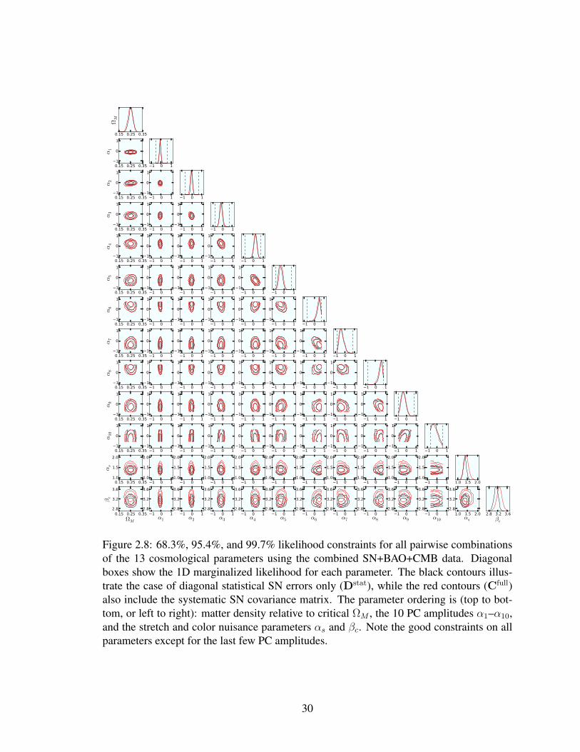
0.15 0.25 0.35

ΩM

0.15 0.25 0.351

0

1

α1

1 0 1

0.15 0.25 0.351

0

1

α2

1 0 11

0

1

1 0 1

0.15 0.25 0.351

0

1

α3

1 0 11

0

1

1 0 11

0

1

1 0 1

0.15 0.25 0.351

0

1

α4

1 0 11

0

1

1 0 11

0

1

1 0 11

0

1

1 0 1

0.15 0.25 0.351

0

1

α5

1 0 11

0

1

1 0 11

0

1

1 0 11

0

1

1 0 11

0

1

1 0 1

0.15 0.25 0.351

0

1

α6

1 0 11

0

1

1 0 11

0

1

1 0 11

0

1

1 0 11

0

1

1 0 11

0

1

1 0 1

0.15 0.25 0.351

0

1

α7

1 0 11

0

1

1 0 11

0

1

1 0 11

0

1

1 0 11

0

1

1 0 11

0

1

1 0 11

0

1

1 0 1

0.15 0.25 0.351

0

1

α8

1 0 11

0

1

1 0 11

0

1

1 0 11

0

1

1 0 11

0

1

1 0 11

0

1

1 0 11

0

1

1 0 11

0

1

1 0 1

0.15 0.25 0.351

0

1

α9

1 0 11

0

1

1 0 11

0

1

1 0 11

0

1

1 0 11

0

1

1 0 11

0

1

1 0 11

0

1

1 0 11

0

1

1 0 11

0

1

1 0 1

0.15 0.25 0.351

0

1

α10

1 0 11

0

1

1 0 11

0

1

1 0 11

0

1

1 0 11

0

1

1 0 11

0

1

1 0 11

0

1

1 0 11

0

1

1 0 11

0

1

1 0 11

0

1

1 0 1

0.15 0.25 0.351.0

1.5

2.0

αs

1 0 11.0

1.5

2.0

1 0 11.0

1.5

2.0

1 0 11.0

1.5

2.0

1 0 11.0

1.5

2.0

1 0 11.0

1.5

2.0

1 0 11.0

1.5

2.0

1 0 11.0

1.5

2.0

1 0 11.0

1.5

2.0

1 0 11.0

1.5

2.0

1 0 11.0

1.5

2.0

1.0 1.5 2.0

0.15 0.25 0.35

ΩM

2.8

3.2

3.6

βc

1 0 1α1

2.8

3.2

3.6

1 0 1α2

2.8

3.2

3.6

1 0 1α3

2.8

3.2

3.6

1 0 1α4

2.8

3.2

3.6

1 0 1α5

2.8

3.2

3.6

1 0 1α6

2.8

3.2

3.6

1 0 1α7

2.8

3.2

3.6

1 0 1α8

2.8

3.2

3.6

1 0 1α9

2.8

3.2

3.6

1 0 1α10

2.8

3.2

3.6

1.0 1.5 2.0αs

2.8

3.2

3.6

2.8 3.2 3.6

βc

Figure 2.8: 68.3%, 95.4%, and 99.7% likelihood constraints for all pairwise combinationsof the 13 cosmological parameters using the combined SN+BAO+CMB data. Diagonalboxes show the 1D marginalized likelihood for each parameter. The black contours illus-trate the case of diagonal statistical SN errors only (Dstat), while the red contours (Cfull)also include the systematic SN covariance matrix. The parameter ordering is (top to bot-tom, or left to right): matter density relative to critical ΩM , the 10 PC amplitudes α1–α10,and the stretch and color nuisance parameters αs and βc. Note the good constraints on allparameters except for the last few PC amplitudes.

30

1 0 1α1

0.190.15

1 0 1α2

0.260.15

1 0 1α3

0.390.32

1 0 1α4

0.430.36

1 0 1α5

0.540.43

1 0 1α6

0.470.47

1 0 1α7

0.610.60

1 0 1α8

0.610.50

1 0 1α9

0.750.77

1 0 1α10

0.930.93

Figure 2.9: Marginalized SN+BAO+CMB constraints on the 10 PC amplitudes. The dashedvertical lines represent the prior limits. Black curves represent constraints from the diag-onal statistical SN errors only, while the red curves correspond to the full SN covariancematrix. The black and red number in each panel shows the ratio of the PC error to therms of the top-hat prior for the statistical-covariance and full-covariance case, respectively.Note the good constraints on all PC amplitudes except for the last few.

(∆αi/√

12)2 term refers to the rms value of the top-hat prior, where ∆αi is the widthof the top-hat prior as calculated in Eq. (2.15).

FoM results are shown in Fig. 2.10, where we show the FoM as a function of the numberof PCs included. The top panel shows the FoMs with and without SN systematic errors,while the bottom panel shows the corresponding ratios of the two cases. We see that theFoM degradation with the addition of SN systematic errors asymptotes to about a factor ofthree to four when about five PCs are included and after that remains relatively constant. Wetherefore conclude that only the few lowest PCs are affected by current systematic errors.We suspect that this is due to the fact that the effect of the systematics is relatively smoothin redshift, and therefore systematics do not become degenerate with the higher PCs thatwiggle in z (see the PC shapes in Fig. 2.7). It is somewhat fortuitous that higher (n & 5)PCs seem to be unaffected by systematics, since it is precisely those higher PCs that aredifficult to measure accurately; however, it may be the case that systematics in future datawill behave differently and affect the higher components.

31

101

102

103

104

105

106

Figu

re o

f Mer

it

1 2 3 4 5 6 7 8 9 10 11 12 13 14 15Number of PCs included

0.00.20.40.60.81.0

FoMfull /

FoMdiag

Figure 2.10: Top panel: FoM as a function of the number of PCs included, with the blackline showing the statistical-only FoM and the red line showing the FoM with systematicsincluded (See Eq. (2.16) for the definition of the FoM). Bottom panel: ratio of the FoM withsystematic errors considered in the SN Ia data to that with only statistical errors considered.BAO and CMB constraints were included in both cases. Notice that the FoM ratio levelsoff after approximately five PCs have been included. Note that here we have consideredthe first 15 PCs (as opposed to 10 in Figs. 2.7-2.9) to show that the FoM indeed flattens offas the PCs become very poorly constrained.

32

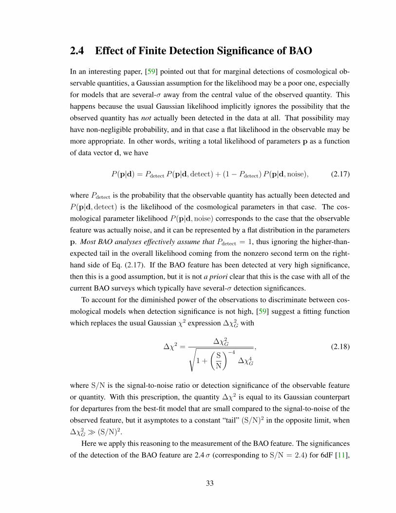
2.4 Effect of Finite Detection Significance of BAO

In an interesting paper, [59] pointed out that for marginal detections of cosmological ob-servable quantities, a Gaussian assumption for the likelihood may be a poor one, especiallyfor models that are several-σ away from the central value of the observed quantity. Thishappens because the usual Gaussian likelihood implicitly ignores the possibility that theobserved quantity has not actually been detected in the data at all. That possibility mayhave non-negligible probability, and in that case a flat likelihood in the observable may bemore appropriate. In other words, writing a total likelihood of parameters p as a functionof data vector d, we have

P (p|d) = Pdetect P (p|d, detect) + (1− Pdetect)P (p|d, noise), (2.17)

where Pdetect is the probability that the observable quantity has actually been detected andP (p|d, detect) is the likelihood of the cosmological parameters in that case. The cos-mological parameter likelihood P (p|d, noise) corresponds to the case that the observablefeature was actually noise, and it can be represented by a flat distribution in the parametersp. Most BAO analyses effectively assume that Pdetect = 1, thus ignoring the higher-than-expected tail in the overall likelihood coming from the nonzero second term on the right-hand side of Eq. (2.17). If the BAO feature has been detected at very high significance,then this is a good assumption, but it is not a priori clear that this is the case with all of thecurrent BAO surveys which typically have several-σ detection significances.

To account for the diminished power of the observations to discriminate between cos-mological models when detection significance is not high, [59] suggest a fitting functionwhich replaces the usual Gaussian χ2 expression ∆χ2

G with

∆χ2 =∆χ2

G√1 +

(S

N

)−4

∆χ4G

, (2.18)

where S/N is the signal-to-noise ratio or detection significance of the observable featureor quantity. With this prescription, the quantity ∆χ2 is equal to its Gaussian counterpartfor departures from the best-fit model that are small compared to the signal-to-noise of theobserved feature, but it asymptotes to a constant “tail” (S/N)2 in the opposite limit, when∆χ2

G (S/N)2.Here we apply this reasoning to the measurement of the BAO feature. The significances

of the detection of the BAO feature are 2.4σ (corresponding to S/N = 2.4) for 6dF [11],

33

ΩM

w

0.1 0.2 0.3 0.4 0.5

−2.5

−2

−1.5

−1

−0.5

ΩM

w

0.22 0.24 0.26 0.28 0.3 0.32 0.34−1.5

−1.4

−1.3

−1.2

−1.1

−1

−0.9

−0.8

−0.7

BAO-only BAO+CMB+SN

Accounts for Finite

Detection Significance

Figure 2.11: Effects on the BAO-only (left panel) and BAO+CMB+SN (right panel) con-straints in the ΩM–w plane with (red) and without (shaded blue) the finite detection signif-icances of the BAO features taken into account. Note that the differences are modest in theBAO-only case and negligible in the combined case.

2.8σ for WiggleZ [41] (combined for three redshift bins), 3.6 σ for SDSS [39] (combinedfor two redshift bins), and 5.0σ for BOSS [43]. We expect that, once the probability ofnon-detection of the BAO feature has been included, the BAO constraints will change,especially for surveys with lower significance of detection and for 99.7% contour regions.This has in fact been confirmed by [59] for the case of the SDSS BAO data alone.

Fig. 2.11 shows the BAO-only (left panel) and BAO+CMB+SN (right panel) constraintsin the ΩM–w plane with and without the finite detection of the BAO features taken intoaccount4. Note that the difference is modest in the BAO-only case and negligible in thecombined case. This is as expected, especially given that some of the strongest BAO datasets (e.g. BOSS) also have the highest detection significances of the BAO feature.

Note also that there is nothing BAO-specific to the effects of the finite detection signif-icance. While the CMB is detected with very high confidence and thus does not warranta similar analysis, it could be applied to SNe Ia where, for example, a few percent of SNemay not be Type Ia5. Given the full probabilistic classification of each SN on whetheror not it is Type Ia [60, 61], one could carry out a similar analysis, which in this contextwould be how imperfect purity of the SN Ia sample affects the constraints on cosmologi-cal parameters. We suspect the results would be even less discrepant relative to the usual

4The results in the w0–wa plane are qualitatively similar, and we do not show them here.5[17] find that the fraction of non-Ia SNe rises from zero at low redshift to O(10%) at z ∼ 1; however,

their modeling is very conservative, and the true fraction of non-Ia SNe is likely very small in the current datasets.

34

perfect-detection analysis than in the case of BAO, and we do not pursue such an analysisin this paper.

In conclusion, the finite detection significance of the BAO feature in large-scale struc-ture surveys leads to a small but discernible weakening of the constraints on cosmologicalparameters.

2.5 Conclusions

In this paper, we have investigated the effects of systematic errors in current SN Ia ob-servations on DE parameter constraints. We accounted for the systematic errors in SNIa observations, including the effects of photometric calibration, dust, color, gravitationallensing, and other systematics by adopting a fully off-diagonal covariance matrix between∼ 500 SNe from the SNLS compilation (see Fig. 2.2). We extended the similar analysisfrom [17] by constraining the temporal evolution of the equation of state of DE describedby the pair of parameters (w0, wa) as well as a much richer description in terms of 10 PCsof the equation of state (shown in Fig. 2.7). We combined the SN Ia constraints with datafrom BAO from four different surveys (see Fig. 2.3) as well as the principal informationon DE given by the acoustic peak measurements of the CMB anisotropies measured by theWMAP experiment.

The constraints on the simple parametrizations of DE are affected by the systemat-ics, but the overall constraints are still strong even after their inclusion (see Figs. 2.4 and2.6). More importantly, we found that systematic errors affect the constraints somewhat,reducing the w0–wa FoM by a factor of about three (see Table 2.3), while the general-ized PC-based FoM is degraded by a factor of three to four (see Fig. 2.10). However, asthe PC analysis shows, this degradation is mainly restricted to the first few numbers (PCamplitudes) describing DE. In fact, what is particularly impressive about current data isthat roughly five PCs are well-constrained even in the presence of systematic errors (seeFigs. 2.8 and 2.9).

In the spirit of testing for systematic effects in current data constraining DE, we alsowondered if the relatively low detection significances of BAO features, ranging from about2.4σ to 5.0σ in various surveys, change the overall cosmological constraints. While nota systematic error per se, the small but non-negligible probability that the BAO featurehas not been detected in some of these surveys implies that the posterior probability ofcosmological parameter values asymptotes to a small but nonzero value far from the like-lihood peak [59]. We find that, while the BAO-only constraints are somewhat affected, thecombined constraints are not (see Fig. 2.11).

35

From all this, we conclude that current systematic errors do degrade DE constraints andFoMs, but not in a major way. Given that future constraints are forecasted to be much better,continued control of current systematic errors remains key for progress in characterizingDE.

36

CHAPTER 3

Distance Probes and Evidence for Phantom DarkEnergy

3.1 Introduction

A key question in understanding the mechanism behind the acceleration of the Universe isthe value of the dark energy equation of state, the ratio of pressure to energy density fordark energy: w ≡ pDE/ρDE . Measurements so far [18–20, 22–25, 62–66] have generallybeen in good, even excellent, agreement with w = −1, the value corresponding to thevacuum energy density described by the famous cosmological-constant term in Einstein’sequations of general relativity. Any measured departure from this value would not onlyprofoundly shake up our understanding of the Universe, but also provide an important hintin our quest to understand cosmic acceleration.

It is therefore particularly important to measure the equation of state and search for anyevidence of its variation in time. Over the past decade, there were several clear instancesin which the measurements indicated that w < −1 at & 2σ evidence [28, 67–69], thougheventually these departures either were explained by known systematics in the data or qui-etly went away as new and better data became available. More recently, with the release ofthe first results from Planck [7], other such claims have been presented, such as [70], whichfeatures high-quality data and a careful analysis including systematic errors [71] (see also[72, 73]). This motivates us to investigate the current data in some detail, concentratingespecially on the value of w marginalized over other cosmological parameters.

The principal tool for studying the equation of state is the combination of three ofthe most mature probes of dark energy: Type Ia supernovae (SNe Ia), baryon acousticoscillations (BAO), and cosmic microwave background (CMB) anisotropies. SNe Ia andBAO probe expansion at low and intermediate redshifts and are thus a crucial ingredientin studying dark energy. The CMB measurements effectively probe a single high-redshiftdistance (specifically, the distance to the surface of last scattering), which is crucial mainly

37

because it provides complementary information to break degeneracy in the Ωm–w plane.For comprehensive reviews of dark energy probes, see [15, 16].

The rest of the paper is organized as follows. In Sec. 3.2, we describe the SN Ia, BAO,and CMB data that we use in our analysis. In Sec. 3.3, we present our results for theconstraints on a constant dark energy equation of state along with several further analysesthat were performed. In Sec. 3.4, we summarize and discuss our findings.

3.2 Data Sets

We begin by describing the data sets used in this analysis. We have used the three most ma-ture probes of dark energy: SNe Ia, BAO, and CMB anisotropies. We focus on these threeprobes since they remain the most mature, well-studied, and robust dark energy probes atpresent. Furthermore, they are expected to be statistically independent for all practical pur-poses. Finally, being purely geometric in nature, they measure dark energy only through itseffect on expansion history; therefore they are understood intuitively and may bypass cer-tain systematic effects, such as those involved in growth of structure measurements, whichare not very well understood.

3.2.1 SN Ia data

SNe Ia were used to discover dark energy [8, 9] and still provide the best constraints ondark energy. SNe Ia are very bright standard candles that are useful for measuring cosmicdistances.

SNe Ia constrain cosmology by providing essentially one measurement each of theluminosity distanceDL(z) = (1+z) r(z) to the redshift of the SN. The theoretical apparentmagnitude is then given by

mth(z) = 5 log10

(H0

cDL(z)

)+M , (3.1)

where the constant magnitude offsetM is a nuisance parameter that depends on both theabsolute magnitude of a SN Ia and the Hubble constant H0. It has long been known thatthere exist useful correlations between the peak absolute magnitude of a SN Ia and boththe stretch (or broadness) and photometric color of its light curve. Simply put, a broaderor bluer SN light curve corresponds to a brighter SN. Thus we compare the theoretical

38

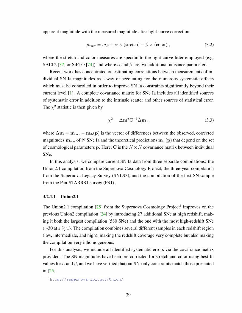
apparent magnitude with the measured magnitude after light-curve correction:

mcorr = mB + α× (stretch)− β × (color) , (3.2)

where the stretch and color measures are specific to the light-curve fitter employed (e.g.SALT2 [37] or SiFTO [74]) and where α and β are two additional nuisance parameters.

Recent work has concentrated on estimating correlations between measurements of in-dividual SN Ia magnitudes as a way of accounting for the numerous systematic effectswhich must be controlled in order to improve SN Ia constraints significantly beyond theircurrent level [1]. A complete covariance matrix for SNe Ia includes all identified sourcesof systematic error in addition to the intrinsic scatter and other sources of statistical error.The χ2 statistic is then given by

χ2 = ∆mᵀC−1∆m , (3.3)

where ∆m = mcorr −mth(p) is the vector of differences between the observed, correctedmagnitudes mcorr ofN SNe Ia and the theoretical predictions mth(p) that depend on the setof cosmological parameters p. Here, C is the N×N covariance matrix between individualSNe.

In this analysis, we compare current SN Ia data from three separate compilations: theUnion2.1 compilation from the Supernova Cosmology Project, the three-year compilationfrom the Supernova Legacy Survey (SNLS3), and the compilation of the first SN samplefrom the Pan-STARRS1 survey (PS1).

3.2.1.1 Union2.1

The Union2.1 compilation [25] from the Supernova Cosmology Project1 improves on theprevious Union2 compilation [24] by introducing 27 additional SNe at high redshift, mak-ing it both the largest compilation (580 SNe) and the one with the most high-redshift SNe(∼30 at z & 1). The compilation combines several different samples in each redshift region(low, intermediate, and high), making the redshift coverage very complete but also makingthe compilation very inhomogeneous.

For this analysis, we include all identified systematic errors via the covariance matrixprovided. The SN magnitudes have been pre-corrected for stretch and color using best-fitvalues for α and β, and we have verified that our SN-only constraints match those presentedin [25].

1http://supernova.lbl.gov/Union/

39

3.2.1.2 SNLS3

Results from the first three years of the Supernova Legacy Survey include measurements of∼250 SNe at intermediate-to-high redshifts. When combined with∼100 low-redshift SNe,∼100 SNe from the Sloan Digital Sky Survey (SDSS), and∼10 high-redshift SNe from theHubble Space Telescope, they produce a compilation [17] of 472 SNe with good redshiftcoverage out to z ∼ 1 and some SNe extending to z ' 1.4. The SNLS3 compilationcontains the largest homogeneous sample and includes many of the best-measured SNealong with a detailed analysis of systematic errors [17]. Note that the SNLS3 and SDSSsamples have been recalibrated [75] and that new cosmological results, including the fullSDSS sample, are forthcoming.

We use the SN Ia data and covariance matrices provided2 to compute the full covariancematrix, which includes all identified sources of statistical and systematic error. Like thecorrected SN magnitudes, the covariance matrix is a function of the light-curve nuisanceparameters α and β. For practical reasons, and for a fairer comparison with other SN Ia datasets, we fix these parameters at their best-fit values (α = 1.43, β = 3.26) throughout theanalysis. It is worth noting that completely marginalizing over these parameters (varyingthem both when computing the corrected magnitudes and when building the covariancematrix) has a negligible effect on constraints in our parameter space. We verify that ourSN-only constraints match those in [1, 17], where α and β are varied.

It is important to note that, in constraints with SNLS3, we follow the prescription in [17]and marginalize over a model with two distinctM parameters, where a mass cut (1010M)of the host galaxy dictates which M applies. This is meant to correct for environmentaldependencies of SN Ia magnitudes on host galaxy properties and is empirical in nature. Wediscuss and investigate this issue further in Sec. 3.3.3.

3.2.1.3 PS1

The primary goal of the Panoramic Survey Telescope and Rapid Response System (Pan-STARRS) is to detect Solar System objects by making precise, repeated observations ofa wide field of view. These observations also lead to the discovery of SNe Ia, which canbe spectroscopically confirmed in follow-up observations. Recently-published SN resultsfrom the first 1.5 years of the Pan-STARRS1 Medium Deep Survey include a compilation[70] of 313 SNe, 112 of which were discovered via Pan-STARRS. The rest (201 SNe)come from a combination of low-redshift samples. Aside from the low-redshift anchor, allSNe come from the same instrument, making this compilation very homogeneous. A full

2https://tspace.library.utoronto.ca/snls

40

systematic analysis is described in [71]. Due to the smaller number of SNe and the lackof high-redshift SNe, the PS1 compilation is not competitive with current constraints fromUnion2.1 or SNLS3, but the survey is ongoing and this will eventually change. The currentcompilation nevertheless provides good constraints on a constant-w model of dark energywhen combined with other probes, so we study it here.

We use the SN Ia data provided3 and adopt the covariance matrix to account for allidentified systematic errors. As with Union2.1, the SN magnitudes have been pre-correctedfor stretch and color, and we have verified that our SN-only constraints agree with those in[70].

3.2.2 BAO data

Baryon acoustic oscillations (BAO) are the regular, periodic fluctuations of visible matterdensity in large-scale structure (LSS) resulting from sound waves propagating in the earlyUniverse. In recent years, measurements of BAO have proven to be useful geometric probesof dark energy. A measurement of the position of the BAO feature in the LSS powerspectrum or correlation function basically provides a precise measurement of a spherically-averaged comoving distance to the effective redshift of the survey. New measurementsover a wide range of redshifts are making it possible to map expansion history with theBAO distance, analogous to the way SNe Ia map expansion with luminosity distance. Forour BAO constraints, we combine recent measurements of the BAO feature from the Six-degree-Field Galaxy Survey (6dFGS) [11], the SDSS Luminous Red Galaxies (SDSS LRG)[76], and the SDSS-III DR9 Baryon Oscillation Spectroscopic Survey (BOSS) [43].

Different authors report their measurement of the BAO feature using different dis-tilled observable quantities. The surveys included here report constraints on the quantityrs(zd)/DV (z) or its inverse, where rs(zd) is the comoving sound horizon at the redshift ofthe baryon drag epoch and DV is a spherically-averaged (two tangential and one radial)distance measure [10] given by

DV (z) ≡[(1 + z)2D2

A(z)cz

H(z)

]1/3

, (3.4)

where DA(z) = r(z)/(1 + z) is the angular diameter distance. We compute the sound

3http://wachowski.pha.jhu.edu/˜dscolnic/PS1_public/

41

horizon via

rs(z) =

∫ t

0

csa

dt′ =∫ a

0

csa′2H(a′)

da′ , (3.5)

cs =c√

3 (1 +R),

where the sound speed cs depends on the ratio of baryon energy density to photon energydensity, which is proportional to the scale factor:

R ≡ 3ρb4ργ≈ 31500 Ωbh

2

(TCMB

2.7 K

)−4

a . (3.6)

The redshift of the baryon drag epoch is given by the fitting formula [77]

zd =1291 (Ωmh

2)0.251

1 + 0.659 (Ωmh2)0.828

[1 + b1(Ωbh

2)b2], (3.7)

where

b1 = 0.313 (Ωmh2)−0.419

[1 + 0.607 (Ωmh

2)0.674],

b2 = 0.238 (Ωmh2)0.223 .

It is important to include a term for radiation in H(a). One can write Ωr = Ωmaeq, whereaeq = 1/(1 + zeq) is the scale factor at the epoch of matter-radiation equality and zeq isapproximated by

zeq ≈ 25000 Ωmh2

(TCMB

2.7 K

)−4

. (3.8)

We assume the value TCMB = 2.7255 K in our analysis.The measured values of the BAO parameters are summarized in Table 3.1. Covari-

ance between different surveys should be negligible here, so we treat these as independentmeasurements.

Note that previous measurements of the BAO feature from SDSS LRG data (e.g.[10, 39]) cannot be used simultaneously with the measurement from [76] since roughlythe same galaxy sample is analyzed. The measurement from [76] makes use of a recon-struction technique to enhance the BAO signal and increase the precision of the distancemeasurement. We use this measurement since it is the most precise and avoids the cor-relation between the pair of measurements from [39], where the SDSS LRG sample iscombined with the SDSS main galaxy sample.

Also note that we choose to leave out the BAO measurements from the WiggleZ

42

Sample zeff Parameter Measurement

6dFGS 0.106 rs(zd)/DV (zeff) 0.336± 0.015

SDSS LRG 0.35 DV (zeff)/rs(zd) 8.88± 0.17

BOSS 0.57 DV (zeff)/rs(zd) 13.67± 0.22

Table 3.1: Summary of BAO measurements combined in the analysis. We list the surveyfrom which the measurement comes, the effective redshift of the survey, the observableparameter constrained, and its measured value.

w

Lik

elih

oo

d

−1.3 −1.2 −1.1 −1 −0.9 −0.80

1

2

3

4

5

6 Planck + BAO

+ PS1

+ Union2.1

+ SNLS3

w

−1.3 −1.2 −1.1 −1 −0.9 −0.8

WMAP9 + BAO

+ PS1

+ Union2.1

+ SNLS3

Figure 3.1: Likelihood curves for a constant equation of state w in a flat universe, usingPlanck CMB data (left panel) and WMAP9 CMB data (right panel). We compare con-straints from CMB + BAO data alone (dashed black) to those which additionally includeSN Ia data from SNLS3 (blue), Union2.1 (green), or PS1 (dashed red). All likelihoods aremarginalized over other cosmological and nuisance parameters, as explained in the text.

Dark Energy Survey [41], which measures the BAO distance in three redshift slices(zeff = 0.44, 0.6, 0.73). These measurements are somewhat correlated with the BOSS mea-surement due to overlap in sky area and redshift, and so far no correlation coefficientshave been estimated. Although the correlation is probably negligible (in part due to shotnoise), adding the WiggleZ measurements to the other BAO measurements improves ourconstraints only very slightly, so we leave them out.

3.2.3 CMB data

Although the CMB contains relatively little geometric information about dark energy, theposition of the first peak in the power spectrum basically provides one very precise mea-surement of the angular diameter distance to recombination at z ≈ 1100. This measure-ment helps break degeneracy between the dark energy equation of state and Ωm [44]. In

43

our analysis, we include CMB constraints from Planck [7] and also from WMAP9 [78] forcomparison.

We summarize CMB information using the following CMB observables:

la ≡ π (1 + z∗)DA(z∗)

rs(z∗), (3.9)

R ≡√

ΩmH20

c(1 + z∗)DA(z∗) . (3.10)

The redshift z∗ of decoupling is given by the fitting formula [79]

z∗ = 1048[1 + 0.00124 (Ωbh

2)−0.738]

(3.11)

×[1 + g1(Ωmh

2)g2],

where

g1 =0.0783 (Ωbh

2)−0.238

1 + 39.5 (Ωbh2)0.763,

g2 =0.560

1 + 21.1 (Ωbh2)1.81.

Following [80], we use the Markov chains from the Planck Legacy Archive (PLA) toderive constraints on the parameter combination (la , R , z∗), which is known to efficientlysummarize CMB information on dark energy, with the measurements themselves indepen-dent of the dark energy model to a good approximation. We assume the same model that weconstrain in this analysis (flat universe, constant w) when deriving the CMB observables.For the Planck data, we use information from the temperature power spectrum combinedwith WMAP polarization at low multipoles (Planck + WP). We also use the PLA chains toderive the corresponding measurements for WMAP9 (temperature and polarization data)with the same model assumptions. The CMB measurements are summarized in Table 3.2.

We evaluate the correlation matrix for (la , R , z∗) for Planck to be 1.0000 0.5262 0.4708

0.5262 1.0000 0.8704

0.4708 0.8704 1.0000

.

44

x± σ Planck WMAP9

la 301.65± 0.18 301.98± 0.66

R 1.7499± 0.0088 1.7302± 0.0169

z∗ 1090.41± 0.53 1089.09± 0.89

Table 3.2: Mean values and standard deviations of the CMB measurements used in ouranalysis. The measurements for both Planck and WMAP9 were obtained using the Markovchains provided by the Planck collaboration. We assumed the model with a flat universeand constant dark energy equation of state, the same model we constrain in this analysis.

The same correlation matrix for WMAP9 is 1.0000 0.4077 0.5132

0.4077 1.0000 0.8580

0.5132 0.8580 1.0000

.

We have explicitly verified that, when multiple probes are combined, the constraintson w obtained directly from the CMB chains are in good agreement with results obtainedusing the measurements in Table 3.2. For the base case of Planck combined with BAO andSNLS3 SNe, the best-fit values of w differ by less than 0.1σ. The discrepancy is greaterwhen the complementary SN data are not included, but the difference is still less than 0.3σfor the data combinations we consider.

Note that our measurements cannot be directly compared to those presented in [80]because of different assumptions: we do not include Planck lensing information, we assumea flat model with w as a free parameter instead of a Λ model with curvature, and we treatz∗ as an observable in place of Ωbh

2.

3.3 Results

3.3.1 Constraint methodology

The complete parameter set used in our analysis is

pi ∈ Ωm , w ,Ωmh2 ,Ωbh

2 , Mi ,

45

z

∆〈M

corr

B〉

0 0.5 1 1.5−0.12

−0.1

−0.08

−0.06

−0.04

−0.02

0

M5 , M6

M3 , M4

M1 , M2

Figure 3.2: Evolution of the mass step predicted from a toy model calibrated using datafrom the Nearby Supernova Factory. This is similar to Fig. 11 of Rigault et al. (2013),though we include a region of uncertainty by propagating errors in the mass step and lo-cal star-forming fraction measured at z = 0.05 from the Nearby Supernova Factory data.Vertical lines separate the three redshift bins, each of which contains two M nuisanceparameters, one for each host galaxy mass range.

where we marginalize over Ωmh2 and Ωbh

2 for the CMB and BAO constraints and over oneor more SN Ia nuisance parametersMi (see Secs. 3.2.1.2 and 3.3.3). Given the small num-ber of parameters, we calculate constraints using brute-force computation of likelihoodsover a grid of parameter values. We assume a Gaussian likelihood L ∝ exp(−χ2/2),where we have ignored the 1/

√det C prefactor, which is a constant and thus cancels out

in likelihood ratios. Note that, in general, the SN covariance matrix is a function of the SNnuisance parameters. If we were to vary those parameters, we would need to recompute theSN covariance matrix at each step; however, one might still want to drop the Gaussian pref-actor, as it can bias the values of recovered parameters if included (e.g. [38] and Appendix Bof [17]). Finally, note that aside from the implicit prior that Ωm ,Ωmh

2 ,Ωbh2 ≥ 0, we

assume flat priors on all of the parameters.

3.3.2 Basic constraints

Combined constraints on the equation of state, marginalized over the other parameters, areshown in Fig. 3.1, where the left panel shows the Planck data combined with the BAOand SN Ia data, while the right panel shows the same for WMAP9. CMB and BAO data

46

Ωm

w

0 0.1 0.2 0.3 0.4 0.5 0.6 0.7

−3

−2.5

−2

−1.5

−1

−0.5

SNLS3 – 6 M

SNLS3 – 2 M

Planck + BAO

Ωm

w

0.26 0.27 0.28 0.29 0.30 0.31 0.32

−1.25

−1.2

−1.15

−1.1

−1.05

−1

−0.95

1 M

2 M

6 M

Planck + BAO + SNLS3

Figure 3.3: Effect of allowing for evolution of the mass step in redshift bins in the SN Iaanalysis. Left: 68.3%, 95.4% and 99.7% likelihood contours in the Ωm–w plane for SNLS3data analyzed the standard way with twoM nuisance parameters (filled blue) and a newway with sixM parameters (open red), one for each of two mass bins and three redshiftbins. Planck + BAO constraints (open black) are overlaid for comparison. Right: 68.3%contours in the same plane for combined Planck + BAO + SNLS3 data using one, two, orsixM parameters.

alone constrain the equation of state rather weakly. With Planck, there is a preference forw < −1, but at ' 1σ it is not significant. There is no preference at all with WMAP9. Notealso that the constraints with Planck are visibly better than those with WMAP9, as Planckmeasures all of the CMB distance parameters (la , R , z∗) more precisely, with errors thatare 2–3 times smaller.

Things get more interesting when SN Ia data are added. The Union2.1 data set pro-duces the best constraints when combined with CMB and BAO, marginally better than theconstraints with SNLS3. Again, though, this leads to good agreement with a cosmologicalconstant, with an insignificant preference for w < −1 driven by the Planck data. However,when SNLS3 or PS1 data are used, we find a preference for w < −1 at the 1.8σ (SNLS3)or 1.9σ (PS1) level with Planck and the 1σ (SNLS3) or 1.2σ (PS1) level with WMAP9.4

Note that the PS1 data give slightly stronger evidence for w < −1, even though the overallconstraints are weaker.

It is useful to study the SN Ia constraints in more detail, which we do in the following

4Since the posterior likelihoods are not perfectly Gaussian, we always determine σ values by computingthe integral of the likelihood between the two values of w where the likelihood equals that at w = −1.The quoted multiple of σ is the number of standard deviations that enclose this probability in a Gaussiandistribution.

47

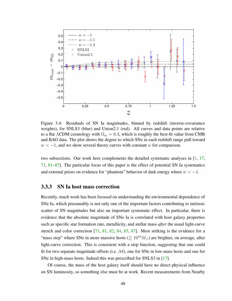
z

mcorr−

mth

0 0.25 0.5 0.75 1 1.25 1.5

−0.5

−0.4

−0.3

−0.2

−0.1

0

0.1

0.2

0.3

0.4

0.5 w = −1

w = −1.1

w = −1.2

SNLS3

Union2.1

Figure 3.4: Residuals of SN Ia magnitudes, binned by redshift (inverse-covarianceweights), for SNLS3 (blue) and Union2.1 (red). All curves and data points are relativeto a flat ΛCDM cosmology with Ωm = 0.3, which is roughly the best-fit value from CMBand BAO data. The plot shows the degree to which SNe in each redshift range pull towardw < −1, and we show several theory curves with constant w for comparison.

two subsections. Our work here complements the detailed systematic analyses in [1, 17,71, 81–87]. The particular focus of this paper is the effect of potential SN Ia systematicsand external priors on evidence for “phantom” behavior of dark energy where w < −1.

3.3.3 SN Ia host mass correction

Recently, much work has been focused on understanding the environmental dependence ofSNe Ia, which presumably is not only one of the important factors contributing to intrinsicscatter of SN magnitudes but also an important systematic effect. In particular, there isevidence that the absolute magnitude of SNe Ia is correlated with host galaxy propertiessuch as specific star formation rate, metallicity, and stellar mass after the usual light-curvestretch and color correction [71, 81, 82, 84, 85, 87]. Most striking is the evidence for a“mass step” where SNe in more massive hosts (& 1010M) are brighter, on average, afterlight-curve correction. This is consistent with a step function, suggesting that one couldfit for two separate magnitude offsets (i.e.M), one for SNe in low-mass hosts and one forSNe in high-mass hosts. Indeed this was prescribed for SNLS3 in [17].

Of course, the mass of the host galaxy itself should have no direct physical influenceon SN luminosity, so something else must be at work. Recent measurements from Nearby

48

Supernova Factory data [87] have indicated strong (∼ 3.1σ) evidence that SNe Ia in locally

passive environments are brighter on average than those in active star-forming environ-ments. The authors further show that this can explain the observed mass step, as passiveenvironments are more common in high-mass galaxies. This is especially important be-cause the fraction of SNe Ia in locally star-forming environments surely evolves with red-shift, and therefore the amplitude of the mass step should also evolve. This is a systematiceffect not corrected for by the introduction of twoM parameters, and the authors estimatea bias on the equation of state of ∆w ' 0.06.

Fig. 3.2 shows a toy model for the redshift evolution of the mass step from the analysisof [87], with errors that we have estimated by propagating errors in the mass step and localstar-forming fraction measured at z = 0.05 from the Nearby Supernova Factory data. Giventhe astrophysical uncertainties in linking the star formation rate to host stellar mass and thelatter to absolute magnitude of SNe Ia, we do not try to use any fixed model to correct forthis. Instead, we use a less model-dependent parametrization of the relation between theobserved host galaxy mass and absolute magnitude by allowing for two independent valuesof M in each of three redshift bins: z ≤ 0.5, 0.5 < z ≤ 1.0, and z > 1.0. Therefore,instead of two offset parameters in the Hubble diagram as in [17], we now have a total ofsixM parameters. The redshift extent that pairs of these parameters cover is illustrated inFig. 3.2, with the divisions centered on the fiducial model presented in [87]. Clearly, oncetheir amplitudes are allowed to float, these nuisance parameters will do a much better jobrecovering the redshift dependence of the mass step than a single pair of M parametersfor the whole redshift range. We succeeded in marginalizing analytically over these sixparameters with flat priors and including covariance between SNe with different M (seeSec. A).

The result is shown in Fig. 3.3. In the left panel, the filled blue contours show the68.3%, 95.4% and 99.7% constraints for the usual case with two M parameters, whilethe open red contours show the result for the six M parameters. The constraints clearlyweaken, although not as much as one might expect with four extra parameters introducedat the level of the Hubble diagram. This “self-calibration” serves to effectively protectagainst departures from the standard-candle assumption. Remarkably, when SN Ia data iscombined with CMB and BAO data, the resulting constraints are barely weakened becausethe lengthening of the contours occurs mainly in the direction that is very well constrainedby the complementary data sets. On the other hand, the right panel of Fig. 3.3 showsthat the best-fit value of w is shifted appreciably, illustrating the sensitivity of dark energyconstraints to systematic effects in SN Ia measurements.

49

z

∆w

0 0.25 0.5 0.75 1 1.25 1.5−0.03

−0.02

−0.01

0

0.01

0.02

0.03

log10 (Mhost/M⊙)

∆w

8 9 10 11 12−0.03

−0.02

−0.01

0

0.01

0.02

0.03

s

∆w

0.8 0.9 1 1.1 1.2−0.03

−0.02

−0.01

0

0.01

0.02

0.03

C

∆w

−0.15 −0.1 −0.05 0 0.05 0.1 0.15 0.2−0.03

−0.02

−0.01

0

0.01

0.02

0.03

Figure 3.5: Effect of each individual SNLS3 SN on the combined constraint on the equationof state, as a function of redshift (top left), host galaxy stellar mass (top right), stretch(bottom left), and color (bottom right). The blue points show the shift ∆w in the finalconstraint on w due to each individual SN. The red circles show the combined (summed)pull from each bin in the particular quantity.

3.3.4 Scanning through SN observables

Are SNe in any given redshift range of the SNLS3 compilation responsible for shifting theequation of state to phantom values? We examine this issue in Fig. 3.4, where we showthe residuals in the Hubble diagram relative to w = −1 for SNe binned in ∆z = 0.075

bins. In this analysis, we have assumed the same cosmology for both SNLS3 and Union2.1(Ωm = 0.3, w = −1), where Ωm is roughly the best-fit value from CMB + BAO. Wefix the stretch, color, andM parameters at their best-fit values separately for each SN Iadata set. We see that the two data sets are consistent at the 1σ level in all bins exceptat z ' 0.95, where they are consistent at 2σ. Therefore, the agreement between the twoHubble diagrams seems excellent.

We can get an even more accurate picture of the redshift dependence of SN constraintson the equation of state. The individual points in Fig. 3.5 show the effect of adding a singleSN to the combination of Planck + BAO + SNLS3. For practical purposes,5 we compare themean equation of state rather than the maximum of the likelihood. The red circles denote

5The computed mean value depends on the precise likelihood ratios between different points in a grid ofparameter values, but a simple numerical estimate of the maximum-likelihood value will only reflect changesthat are of order the grid spacing or larger.

50

the total (summed) contribution of SNe per ∆z = 0.075 bin. We see that no redshift bincontributes to a negative shift in the mean equation of state more than about 0.01.

The other three panels in Fig. 3.5 show the individual SNLS3 SN contributions to was a function of stretch, color, and host galaxy stellar mass. As before, the red circlesdenote the summed contribution of all SNe in a given bin in the quantity shown. As in theredshift scan, we do not observe any correlation or particular region in the stretch, color, orhost-mass spaces that is chiefly responsible for shifting the equation of state.

3.3.5 External H0 Prior

Adding a prior corresponding to an external measurement of the Hubble constant with asmall error bar has an important effect on our results. This is easy to understand: Given thatthe CMB essentially pins down the physical matter density Ωmh

2 (for example, to betterthan 2% with Planck), δ ln Ωm ' −2δ lnh and therefore a higher value of H0 correspondsto a lower value of Ωm. For a lower Ωm, the degenerate direction of CMB + BAO con-straints leads to a more negative w. Therefore, we would expect that higher values of H0

lead to more negative w, and vice versa.This expectation is confirmed by our explicit tests with the current data, shown in

Fig. 3.6. Here we use the same Hubble constant measurement error of ±2.4 km/s/Mpcas reported by [88], but instead of adopting the central value of 73.8 km/s/Mpc, we varythe central value as an integer in the range H0 ∈ [65, 75] km/s/Mpc, one value at a time.We show the final constraint on the dark energy equation of state using the CMB + BAO+ H0 data, with or without the addition of the PS1 or SNLS3 SN data, as a function ofthe H0 central value. For the external prior H0 = 74 ± 2.4 km/s/Mpc, we recover resultssimilar to [70] that favor w < −1 at ∼ 2.5σ. However, for a smaller central value of H0

(≤ 70 km/s/Mpc), the results are consistent with w = −1 at the 2σ level or less, and for aneven smaller central value (' 66 km/s/Mpc), we find the results consistent with w = −1 at1σ.

3.4 Conclusions

We studied geometric constraints on the dark energy equation of state from recent SN Iadata complemented with distance measurements from the CMB and a compilation of BAOresults. For the SNLS3 and PS1 SN data sets, the combined SN Ia + BAO + Planck datafavor a phantom equation of state where w < −1 at ∼ 1.9σ confidence (see Fig. 3.1), ingood agreement with the corresponding results reported in the original SN Ia and Planck

51

H0 Central Value (km/s/Mpc)

w

65 66 67 68 69 70 71 72 73 74 75−1.4

−1.3

−1.2

−1.1

−1

−0.9

−0.8 Planck + BAO + H0

+ SNLS+ PS1

Figure 3.6: Effect of an external H0 prior on the constant equation of state. We showthe effect on Planck + BAO constraints (black) and on combined Planck + BAO + SNconstraints separately for PS1 (red) and SNLS3 (blue), where the error bars bound 68.3%and 95.4% of the likelihood for w. The external prior has an uncertainty of 2.4 km/s/Mpcin each case, mimicking the uncertainty in the Riess et al. (2011) measurement.

papers. Evidence for a phantom equation of state is weaker if WMAP9 is used insteadof Planck, while the Union2.1 data set is consistent with the cosmological-constant valuew = −1 when combined with either CMB data set.

We have tested for a possible presence of systematics correlated with SN properties –their redshifts, stretch factors, colors, and host galaxy masses. We find no evidence of atrend or that a particular range of any of these properties contributes to pushing w < −1;rather, the hints of a phantom equation of state appear to be uncorrelated with these basicSN observables. We have also investigated the effect of modeling the redshift dependenceof the host galaxy mass step of SN luminosities, assigning up to six separate M param-eters for different mass and redshift bins. The additional nuisance parameters shift theSN Ia constraints sufficiently that, when combined with BAO and CMB data, they allowagreement with w = −1 at ∼ 1σ. Therefore, a more generous allowance for the temporalevolution of the dependence of SN luminosity on host galaxy mass removes the evidencefor w < −1. The hope for the future is that independent observations can pin down theenvironmental dependence of SN luminosities and make it possible to account for suchsubtle but important systematic effects in a consistent way and without the damaging effectof extra nuisance parameters at the level of the Hubble diagram.

52

External measurements of the Hubble constant play a particularly important role in thefinal constraints on w. This is shown in Fig. 3.6, where we illustrate the effect of addinga measurement of H0 with an error of 2.4 km/s/Mpc as in [88], but with the central valuevaried from 65-75 km/s/Mpc. Clearly, interesting > 2σ evidence for the phantom equationof state is present only when the central value is somewhat large: H0 & 71 km/s/Mpc.Therefore, as first clearly argued by [89], with excellent CMB constraints the Hubble con-stant measurements and their interpretation (e.g. [90, 91]) are among the most importantinputs in determining the dark energy equation of state.

Although we have taken Planck + BAO data at face value throughout most of our anal-ysis, it is worth mentioning that systematics may be present in these data as well. This isparticularly true for the Planck data, given that its analysis is still in the early stages andgiven the moderate tension between Planck results and both WMAP and growth measure-ments (e.g. [92]). Indeed, a recent re-analysis of Planck data [93] resulted in parametershifts that somewhat reduce the tension with WMAP, and substantial ongoing work is fo-cused on understanding systematics in growth measurements.

With current data we therefore find ourselves in an interesting situation in which wecan make the following statement at 2σ confidence: Given Planck data, either the SNLS3and PS1 data have systematics that remain unaccounted for or the Hubble constant is below71 km/s/Mpc; else the dark energy equation of state is indeed phantom.

53

CHAPTER 4

Multiplicative Errors in the Power Spectrum

4.1 Introduction

Observations of large-scale structure (LSS) have proven to be a powerful probe of cos-mology in recent years. Earlier large galaxy surveys, such as CfA [94], APM [95], and2dF [96, 97], have paved the way for modern surveys like WiggleZ [98], SDSS [99–101],and the Baryon Oscillation Spectroscopic Survey (BOSS), the current incarnation of SDSS[102, 103]. These surveys have identified millions of galaxies and obtained spectra (andtherefore redshifts) of over one million, allowing us to map the three-dimensional distri-bution of matter in the Universe. The enormous data sets resulting from these surveys areoften distilled into measurements of the location of the peak in the correlation functioncorresponding to the scale of baryon acoustic oscillations (BAO), the imprint on structureresulting from sound waves propagating in the early Universe [10, 39, 43, 76, 104]. TheseBAO measurements, some of which are now at the percent level [13], have been crucial inthat they complement other probes of cosmic expansion to help break degeneracies betweenkey cosmological parameters.

But there is much more information in the power spectrum than just the primary BAOpeak, and with ongoing surveys like the Dark Energy Survey (DES; Abbott et al. 105),which is on track to identify ∼300 million galaxies, the galaxy power spectrum as a wholewill complement other probes of cosmology (CMB power spectra, Type Ia supernovae,weak lensing, etc.) to place tight constraints on dark energy and other cosmological pa-rameters. Planning is already underway for future wide-field LSS surveys, such as LSST[106] and Euclid [107].

Making these observations suitable for cosmology is not trivial. With the enormousstatistical power of surveys like DES, control of systematics becomes crucial, especiallyat small scales where cosmic variance is small. A major class of systematic errors is pho-

tometric calibration errors, by which we mean any systematic that effectively causes the

54

magnitude limit of the sample to vary across the sky, thus biasing the true galaxy powerspectrum. A number of recent observations [108–114] show a significant excess of powerat large scales that likely results from such calibration errors that have not been accountedfor. Recent work [109, 110, 114–117] has focused on mitigating these systematics in orderto probe the underlying cosmology.

[118], which we will refer to as H13, introduced a formalism for quantifying the effectof an arbitrary photometric calibration error. They found that in order to use informationfrom large scales to constrain cosmological parameters, the root-mean-square variationdue to the calibration field must be ∼0.001–0.01 mag or less in order to avoid significantlybiasing cosmological parameters. This is a very stringent requirement.

A potentially more dangerous effect is the multiplicative leakage of these large-angleerrors to small angular scales, where most cosmological information resides. As discussedin H13, the observed number density of galaxies is given by Nobs(n) = [1 + c(n)]N(n),where the true number density N(n) is modulated by a calibration-error field c(n), whichis directly related to a host of interrelated photometric effects (survey depth, completeness,atmospheric conditions, galactic dust, etc.). Even though the calibration error is significantonly at large angular scales, it multiplies the true galaxy field, so the observed field isaffected on all angular scales. This multiplicative effect, to our knowledge first pointed outin H13 in the context of LSS systematics, is further studied in this work.

Current methods to clean the power spectra have been impressively efficient, but theytypically rely on systematics templates – prior knowledge of the relative spatial variationof the contamination across the sky due to a known systematic. The methods rely onthe assumption that these templates are correct and that the set of templates is complete;any unknown large-scale systematic that is not covered by one of the templates (or somecombination thereof) will not be accounted for.

Mode projection (or extended mode projection, see Leistedt and Peiris 117) is a par-ticularly effective method. Essentially, it is a way of marginalizing over spatially varyingpatterns on the sky that are expected to be caused by various systematics. While modeprojection has been shown to be effective at mitigating the added power from known sys-tematics, this method cannot remove multiplicative errors. To understand why, suppose forsimplicity that a single systematic effect modulates the observed galaxy densities and thatthe shape of the template is that of a pure spherical harmonic (so that c(n) ∝ Y`m(n) forsome `, m). This modulation will then not only add power at the angular scale `, but it willalso affect the power at all other multipoles. The obvious way to “project out” this mode,at least in principle, is to simply ignore that one contaminatedmmode when estimating thevarianceC`. The additive error is removed entirely with little loss of cosmological informa-

55

tion, but other multipoles have still been affected by the multiplicative effect in accordancewith our Eq. (4.13) below.

In this paper, we study a new approach that is both alternative and complementary topreviously employed techniques: using some of the power spectrum observations them-selves to directly measure the systematic contamination and correct the rest of the mea-surements for a cosmological analysis. Since the calibration errors are expected to enter atlarge scales and then fall off quickly at higher multipoles (smaller scales), one may inter-pret the low-multipole power spectrum as measurements of the systematics and use these tocorrect the power spectrum at high multipoles, sacrificing some cosmological informationfrom large scales to remove the multiplicative error and obtain unbiased estimates of cos-mological parameters from small scales. The benefit of this approach is that no templatesor otherwise detailed modelling of the systematics is required at this level.

The rest of the paper is organized as follows. In Sec. 4.2, we review and extend the cal-ibration formalism introduced in H13, discuss our Fisher matrix formalism, and describea fiducial model and DES-like survey. In Sec. 4.3, we quantify the effect of multiplica-tive calibration error for our fiducial survey and demonstrate the self-calibration method.In Sec. 4.4, we summarize our conclusions and discuss how one might apply the self-calibration method to real data.

4.2 Methodology

In this section, we outline our formalism to describe the calibration errors, review andextend the Fisher matrix for the galaxy power spectrum, and detail our fiducial model andsurvey.

4.2.1 Calibration Error Formalism

In the absence of all systematics, we would observe the true number density of galaxies onthe sky, which we expand in spherical harmonics:

δ(n) ≡ N(n)− NN

=∞∑`=0

∑m=−`

a`mY`m(n) , (4.1)

where a bar denotes a sky average and where the monopole vanishes (a00 = 0) since itis proportional to the average overdensity on the sky, which is zero by construction. Thecoefficients a`m are expected to be Gaussian random variables with a mean of zero and avariance that depends on the cosmological model. The various m modes are statistically

56

independent under the assumption of isotropy, so we have the familiar relations

〈a`ma∗`′m′〉 = δ``′ δmm′ C` , (4.2)

〈a`m〉 = 0 . (4.3)

Following H13, we now consider the effect of an arbitrary variation in the limiting magni-tude δmmax(n) of the photometric survey due to calibration variation across the sky. Thismagnitude variation implies a relative variation in galaxy counts [δN/N ](n) ∝ δmmax(n),where the constant of proportionality depends on the faint-end slope of the luminosity func-tion s(z) ≡ d log10N(z,m)/dm|mmax that may depend on redshift but does not depend ondirection. More generally, one can write [δN/N ](n) ≡ c(n) so that the observed galaxynumber density Nobs(n) is equal to the true number density N(n) modulated by the fieldc(n), which we can also expand in spherical harmonics:

Nobs(n) = [1 + c(n)]N(n) , (4.4)

c(n) =∑`m

c`mY`m(n) . (4.5)

The calibration coefficients c`m are deterministic (not inherently stochastic) and thus havethe trivial statistical properties

〈c`mc∗`′m′〉 = c`mc∗`′m′ , (4.6)

〈c`m〉 = c`m . (4.7)

In other words, the calibration-error field is a fixed pattern on the sky, and there is no lossof generality in making this assumption to simplify the analysis. The observed overdensityis given by

δobs(n) ≡ Nobs(n)− Nobs

Nobs=

[1 + c(n)]N(n)

N(1 + ε)− 1

=1

1 + ε[δ(n) + c(n) + c(n)δ(n)− ε] , (4.8)

where Nobs = N(1+ε) is the observed mean number of galaxies per pixel on the sky. Thenε is defined by

ε ≡ 1

Nc(n)N(n) = c(n) [1 + δ(n)] =

c00√4π

+1

4π

∑`m

c`ma∗`m , (4.9)

57

where the overbar again denotes a sky average.Expanding the observed overdensity in spherical harmonics,

δobs(n) =∑`m

t`mY`m(n) , (4.10)

we calculate the expansion coefficients of δobs to be

t`m =1

1 + ε

a`m + c`m −√

4π ε δ`0 +∑`1m1`2m2

R`1 `2 `m1m2m

c`1m1a`2m2

, (4.11)

where the coupling coefficient R`1 `2 `m1m2m

is a variant of the Gaunt coefficient, the result ofintegrating a product of three spherical harmonics. It can be written in terms of Wigner 3-jsymbols:

R`1 `2 `m1m2m

≡ (−1)m√

(2`1 + 1)(2`2 + 1)(2`+ 1)

4π(4.12)

×(`1 `2 `

0 0 0

)(`1 `2 `

m1 m2 −m

).

In this formalism, how will the observed power be related to the true power C`? Ifthe observed coefficients are t`m, then the observed (potentially biased) power is given by(Appendix B)

T` =

∑m〈|t`m|2〉2`+ 1

= C` + Ccal` −

1

2πCcal` C` (4.13)

+1

4π

∑`1`2

(2`1 + 1)Ccal`1

(`1 `2 `

0 0 0

)2

(2`2 + 1)C`2 ,

where we have defined the calibration-error contribution to the observed power as

Ccal` ≡

∑m

|c`m|2/(2`+ 1) . (4.14)

It is worth making several comments about Eq. (4.13), where the observed angular powerspectrum T` is given as a function of the true powerC`, the calibration-error powerCcal

` , andvarious geometric coupling factors. The second term on the right-hand side,Ccal

` , representsthe additive effect of calibration error, which is typically important at large angular scales

58

(such as ` . 20). The other terms are products of the true and calibration-error power;they represent the multiplicative effect of calibration errors that affects the observed powerT` at all angular scales. Note that Eq. (4.13) is equivalent to the formula for T` from H13,though here we have substantially simplified it by defining away the 1/(1 + ε) factor andusing Wigner 3-j relations (see Appendix B for more details).

Finally, we can gain some insight into the multiplicative contribution to T` by simpli-fying Eq. (4.13) under the assumption that Ccal

` vanishes for multipoles greater than somecutoff multipole ` = `max, cal and with the approximation that the true power C` is constantin the multipole range ` ± `max, cal that contributes to the sum over `2. This allows us tofactor C`2 out of the sum and apply the Wigner 3-j relation Eq. (B.8). Then Eq. (4.13)simply becomes

T` ' C` + Ccal` −

1

2πCcal` C` + σ2

c C` , (4.15)

where σ2c ≡ Var[c(n)] =

∑∞`=1(2` + 1)Ccal

` /(4π) is the variance of the calibration fieldacross the sky. This is generally an excellent approximation, and it shows that the multi-plicative effect (the last term) is roughly independent of the shape of the calibration powerspectrum. Also, all C` at ` > `max, cal are multiplied by roughly the same factor, an effectmimicking that of an incorrect galaxy bias.

4.2.2 Fisher matrix and bias

We now review and extend the standard LSS Fisher matrix formalism in order to forecastboth the extent to which multiplicative calibration errors bias cosmological parameters andthe uncertainty that results from trying to measure the contamination itself.

In the absence of systematics, and when cross-power spectra are assumed to vanish(C ij

` ≡ 0 for i 6= j), the observables Cii` are uncorrelated with a variance due to cosmic

sampling variance and shot noise:

Var[Cii` ] =

2

(2`+ 1)fsky

(Cii` +

1

N i

)2

, (4.16)

where N i is the number of galaxies per steradian for redshift bin i. Then the well-knownFisher matrix for measurements of the power spectrum is given by

Fαβ =∑i

∑`

∂Cii`

∂pα

1

Var[Cii` ]

∂Cii`

∂pβ, (4.17)

where the pi are cosmological parameters.

59

We will be particularly interested in the effect of the presence of uncorrected-for cal-ibration errors on cosmological parameters. A useful Fisher-matrix-based formalism isavailable to evaluate these effects [119, 120]. Given a bias δm in a vector of observablesm with covariance matrix C, the linear estimate for the bias in cosmological parameters is

δp = F−1D C−1δm , (4.18)

where the matrix D contains the derivatives of the observables with respect to the parame-ters evaluated at their fiducial values: Dij = ∂mj/∂pi.

We can extend the Fisher matrix to measure both cosmological parameters andcalibration-error parameters Ccal

` from the observed (biased) angular power spectrum. Ourobservables are now the set of T ii` , and we calculate their covariance from Eq. (4.15). To agood approximation, they are uncorrelated with a variance

Var[T`] ' Var[C`](

1 + σ2c −

1

2πCcal`

)2

, (4.19)

where Var[C`] is the usual error from cosmic variance plus shot noise, as in Eq. (4.16),and the redshift bin indices have been suppressed. The derivatives with respect to theparameters are

∂T`∂pi' ∂C`

∂pi

(1 + σ2

c −1

2πCcal`

), (4.20)

∂T`∂Ccal

`′' δ``′

(1− 1

2πC`

)+

2`′ + 1

4πC` . (4.21)

Note that when none of theCcal` are added as parameters, the Fisher matrix for cosmological

parameters reduces to the usual Fisher matrix Eq. (4.17), independent of the fiducial sizeof the calibration errors.

4.2.3 Fiducial model and survey

At small scales, we use the Limber approximation, which ignores the contribution of radialmodes, and model the angular power spectra of galaxy density fluctuations as

Cij` = bibj

∫ ∞0

H(z)

r2(z)P

(`+ 1

2

r(z), z

)W i(z)W j(z) dz , (4.22)

where bi is the galaxy bias for the ith redshift bin (which we assume to be a constant), H(z)

is the Hubble parameter, r(z) is the comoving distance, P (k, z) is the power spectrum, and

60

the weights are given by

W i(z) =n(z)

N i

[θ(z − zimin

)− θ

(z − zimax

)], (4.23)

where θ(x) is the Heaviside step function, zimin and zimax are the lower and upper bound ofthe ith redshift bin, and n(z) is the radial distribution of galaxies per steradian. We usethe transfer functions and nonlinear modelling of CAMB [121] to compute and evolve thepower spectrum.

The Limber approximation is not valid at the largest scales, so for ` ≤ 30, we use thefull expression for the power spectrum:

Cij` =

2

π

∫ ∞0

P (k, 0) I i`(k) Ij` (k) k2dk , (4.24)

I i`(k) ≡ bi∫ ∞

0

W i(z)D(z) j`(k r(z)) dz , (4.25)

where D(z) is the linear growth factor relative to z = 0 (since we are safely in the linearregime) and j`(x) is the spherical Bessel function of order `. Note that in the above we areassuming a flat universe.

Our fiducial DES-like survey covers 5,000 deg2 (corresponding to fsky ' 0.12)and identifies a total of 300 million galaxies ('17 galaxies per arcmin2). We splitthe sample into five tomographic redshift bins of width ∆z = 0.2, centred atz = 0.1, 0.3, 0.5, 0.7, and 0.9. We take the radial distribution of galaxies to be n(z) ∝z2 exp(−z/z0), with z0 = 0.3, and divide the total number of galaxies among the redshiftbins accordingly. As shown in Fig. 4.1, the distribution peaks at z = 2z0 = 0.6. We assumethat the photometric redshifts can be determined well enough that the cross-power spectrabetween these bins are small enough to be ignored, making the power spectra for differentz slices statistically independent.

We choose for our fiducial cosmology a flat ΛCDM model with Ωm = 0.3, Ωmh2 =

0.143, Ωbh2 = 0.0222, ns = 0.96, and 109As = 2.2 for k0 = 0.05 Mpc−1, values which

agree well with data from Planck [7] and other probes.In our analysis, we allow the dark energy equation of state to vary along with the pa-

rameters above, though we keep Ωmh2 and Ωbh

2 fixed at their fiducial values. In prac-tice, Planck CMB measurements constrain these parameters very well (to ∼1%), so weare effectively adding Planck priors to all of our constraints and assuming the remaininguncertainty to be negligible, which should be a reasonable approximation. We assume a(constant) galaxy bias bi = 2.2 (same for all redshift bins), which we hold fixed for simplic-

61

z

n(z)

0 0.2 0.4 0.6 0.8 1 1.2 1.40

0.5

1

1.5

2

2.5

3x 10

8

12

35

4

Figure 4.1: Number density of galaxies per steradian for our fiducial survey. Galaxies areassigned to the five redshift bins in proportion to the areas of the coloured regions, eachspanning ∆z = 0.2.

ity. In a full analysis, one should parametrize the bias appropriately and marginalize, sincethe bias parameters may have significant uncertainties and be somewhat degenerate withcosmological parameters. Allowing the dark energy equation of state to vary with time asw(a) = w0 + wa(1 − a) [52], our fiducial parameter space is therefore five-dimensional(Ωm, w0, wa, ns, As), though we briefly consider a constant equation of state (with fixedwa = 0) as well.

4.3 Results

4.3.1 Biases from multiplicative errors

H13 used a similar formalism to study the effect of arbitrary photometric calibration errorson cosmological parameters. The large biases that resulted were primarily due to additiveerrors (the Ccal

` term in Eq. (4.13)), which strongly biased the power spectrum at low mul-tipoles and which were assumed negligible at smaller scales (Ccal

` = 0 for ` > `max, cal).With the exception of some parameters (e.g. fNL), most of the constraining power on cos-mological parameters, including dark energy parameters, comes from high `, where thereare many more modes to minimize cosmic variance. The simplest way to avoid biases dueto these large additive errors at low ` is to just remove those multipoles from the analysis,sacrificing the modest amount of information they contain. For our fiducial survey, we find

62

ℓ

ℓ(ℓ

+1)C

ℓ/(2π)

102

103

10−3

10−2

10−1

100

Fiducial Spectrum

With Multiplicative Errors

zeff = ,0.1 0.5 0.9,

Figure 4.2: Multiplicative effect due to our fiducial calibration errors with σ2c = 0.1 dis-

tributed on large scales ` ≤ 20. The biased power spectrum T` (black points) is comparedto the true power spectrum C` (solid lines) for three of the five redshift bins of our fidu-cial survey. The spectra are binned in ` with inverse-variance weights, and the error boxesinclude cosmic variance and shot noise.

that this increases the errors on parameters by ∼1%, though this number is sensitive tothe model and which parameters are varied. Alternatively, with detailed modelling of thesystematic effects, one can attempt to remove the contaminated modes and obtain usefulcosmological information from the low multipoles.

The problem is not so simple when there are significant multiplicative errors, corre-sponding to the other terms in Eq. (4.13), where a given multipole is not only affected bycalibration errors at that scale, but also calibration errors from every other multipole. Ig-noring or cleaning the low-` information is not helpful here, since the biases have already“leaked” into the high-` power. The multiplicative errors are much smaller (by a factor oforder C`) than the additive errors, but for a large total amount of contamination, the effectscan be important.

In Fig. 4.2, we show our fiducial power spectra along with the same power spectrawhen biased due to multiplicative errors, for three of the five redshift bins. The spectra are

63

binned with inverse-variance weights, and the error boxes represent the combined cosmicvariance and shot noise error for each bin. For definitiveness, we assume a spectrum forthe calibration systematics of Ccal

` ∝ `−2 (separately for each redshift bin) and impose acutoff such that Ccal

` = 0 for ` > `max, cal = 20. A variance of the calibration-error fieldacross the sky of σ2

c = 0.1 is assumed. Recall that this quantity is related to the powerspectrum of calibration errors by σ2

c ≡ Var[c(n)] =∑∞

`=1(2` + 1)Ccal` /(4π). While this

is a large contamination, it may not be unrealistic for a survey like DES, since the relevanterror is the raw variation in the effective magnitude limit before any attempts to clean orremove it. While the cleaning or marginalization methods effectively remove the additivecontribution, the Ccal

` term in Eq. (4.13), the original multiplicative effects remain.Note that the factor by which the power is increased by the multiplicative errors is

relatively constant, but since cosmic variance decreases at higher `, the biases eventuallybecome larger than the errors. From the approximate expression Eq. (4.15), we can easilyestimate this relative bias in the space of observables. The multiplicative bias is σ2

c C`,while the variance is given by Eq. (4.16). Ignoring the shot noise contribution, the biasrelative to the error is therefore

T` − C`σC`

'√

(2`+ 1) fsky

2σ2c . (4.26)

For σ2c = 0.1, the bias is as large as the error for ` ' 800 and twice as large for ` '

3,000. The biases on bandpowers, such as those shown in Fig. 4.2, are more severe still,as cosmic variance is further reduced by measuring the power spectrum in bins spanningseveral independent ` modes.

Fig. 4.3 shows the effect of the bias from Fig. 4.2 in the space of dark energy parametersw0 and wa using information from ` = 21 through `max = 2,000. In this case, both w0 andwa are shifted from their fiducial values by more than 3σ.

Fig. 4.4 shows the effect of these same biases in the full space of our cosmologicalparameters. We plot ∆χ2 as a function of the maximum multipole `max used in the analysis,where ∆χ2 = δp>F δp. For the five-dimensional space of all parameters, this is equivalentto the observable-space ∆χ2 in the Fisher matrix formalism. In this case, χ2 is shiftedby 3σ for `max ' 100. We also show ∆χ2 for the two-parameter spaces of Ωm and w

(marginalizing over As and ns but fixing wa = 0) and for w0 and wa (marginalizing overthe other three parameters). In these cases, χ2 is shifted by more than 3σ for `max '2,500. Notice that the sizes of the biases oscillate somewhat; since the Fisher derivativessometimes flip sign, the biases will cancel for some `max. This subtlety depends strongly onwhich parameters are of interest, apparent here from the “out-of-phase” cancelling between

64

the constant-w and w0–wa dark energy parametrizations. It is therefore the envelope of thebias curves in the Ωm–w and w0–wa spaces that indicates the bias one can realisticallyexpect.

Although we fix the galaxy bias in this illustration, it is worth mentioning that the effectat high ` of a constant (scale-independent) galaxy bias is almost completely degeneratewith the multiplicative effect from low ` (see Eq. (4.15) with Ccal

` = 0). In other words,if the contaminated low multipoles are removed from the analysis and the galaxy bias isconstrained along with other cosmological parameters, the inferred value of the galaxybias will shift due to the multiplicative effect, but the marginalized constraints on the othercosmological parameters will not be significantly biased. Of course, if the galaxy biasexhibits scale dependence or can be known independently to a good precision (which weeffectively assumed here), this will not be the case.

Figure 4.3: Forecasted 68.3, 95.4, and 99.7 per cent joint constraints on the w0–wa darkenergy parametrization for our fiducial survey, using information from ` = 21 through`max = 2,000 without calibration errors (blue) and with multiplicative calibration errorsfrom ` ≤ 20 with σ2

c = 0.1 (red).

65

ℓmax

∆χ2

101

102

103

104

10−1

100

101

102

103

104

105

Full 5D parameter space

Ωm–w plane

w0–wa plane

Figure 4.4: Shift in parameter-space χ2 due to multiplicative calibration errors as a func-tion of the maximum multipole used in the analysis. We show the effect on the full five-dimensional space of parameters (black) along with the two-dimensional spaces of Ωm andw with fixed wa = 0 (blue) and w0 and wa (red). The overlaid dashed grey lines markthe 68.3, 95.4, and 99.7 per cent bounds for a two-dimensional Gaussian distribution (forcomparison with the red or blue lines).

4.3.2 Self-calibration to remove multiplicative errors

We now study the possibility of measuring the contamination directly at low multipolesto correct the power at high multipoles. Due to large cosmic variance, the low-` Ccal

` arenot known precisely, and for a cut sky, there will be very few modes to inform us aboutthe lowest-` Ccal

` . In practice, the T` would be measured in bandpowers, so one could thenmeasure the calibration error in bandpowers, but for our purposes here, we assume that eachCcal` can be measured with an associated error due to cosmic variance of the true power (and

shot noise, though it is negligible at the relevant low multipoles). Note that in our Fisherformalism we are ignoring any additional errors that may result from imperfectly extractingT` from the cut sky, though these could be estimated in principle [116, 122, 123].

To study the effect of a self-calibration procedure, we consider the example inSec. 4.3.1, where a calibration power spectrum Ccal

` ∝ `−2 with σ2c = 0.1 and `max, cal = 20

has been added to each of the fiducial power spectra. We introduce the Ccal` as nuisance

parameters to be constrained along with the cosmological parameters. Since `max, cal = 20,there are 20 calibration-error parameters for each of five redshift bins, for a total of 100nuisance parameters. Using the Fisher matrix formalism discussed in Sec. 4.2.2, we can

66

ℓmax

∆χ2

102

103

0

5

10

15

20

25

30

35

40

20

5

10

ℓmax,meas =

20

15

18

Figure 4.5: Shift in the full five-dimensional parameter-space χ2 due to multiplicative cali-bration errors as a function of the maximum multipole used in the analysis, for calibration-error parameters measured up to various `max, meas. The overlaid dashed grey lines mark the68.3, 95.4, and 99.7 per cent bounds for a five-dimensional Gaussian distribution.

estimate the additional statistical error on cosmological parameters that results from imper-fectly measuring the Ccal

` .In Fig. 4.5, we show the effect of measuring Ccal

` up to a variety of `max, meas by plot-ting ∆χ2 (in the five-dimensional parameter space of Ωm, w0, wa, ns, and As) due to theremaining bias, as a function of the maximum multipole `max used in the analysis. In otherwords, for `max, meas = x, we constrain 5x total nuisance parameters. For `max, meas = 20,∆χ2 = 0 for all `max, since the assumption is that all of the calibration terms have beenmeasured without significant bias. Note the very large biases in the cosmological parame-ters when `max, meas is low; that is, when we have not used measurements of additive errorat sufficiently many low multipoles to effectively “clean” the high-multipole LSS informa-tion.

In Fig. 4.6, we show the statistical error and remaining bias in thew0 andwa dark energyparameters as a function of the maximum multipole `max, meas at which calibration errors aremeasured. For both parameters, the statistical errors increase modestly (by ∼50%), whilethe biases approach zero at `max, meas = `max, cal. In this specific case, it is apparent that onewould need to measure systematics to ` ' 10 in order to reduce the biases to a comfortablelevel (such as ∼1/4 of the statistical error).

67

ℓmax,meas

∆w

0

0 2 4 6 8 10 12 14 16 18 200

0.02

0.04

0.06

0.08

0.1

0.12

0.14

0.16

Error

Bias

ℓmax,meas

∆w

a

0 2 4 6 8 10 12 14 16 18 200

0.1

0.2

0.3

0.4

0.5

0.6

Error

Bias

Figure 4.6: Statistical error (blue) and bias (dashed red) on w0 (left) and wa (right) as afunction of the maximum multipole `max, meas at which calibration errors are measured.

4.4 Discussion

In this paper, we have considered a general class of systematic errors – photometric cal-ibration errors – that contaminate measurements of the galaxy angular power spectrum.These errors arise from any effect which causes a spatial variation in the effective mag-nitude limit of the photometric survey, modulating the true galaxy number densities andbiasing the angular power spectrum (see Eq. (4.13)). More specifically, we studied the ef-fect of multiplicative errors, where calibration error at any scale biases inferences of thepower spectrum at all other scales. In this case, cleaning the power spectra of excess ad-ditive power, or excluding contaminated multipoles from the analysis, does not remove themultiplicative effect. For a large total amount of contamination, the multiplicative effectcan significantly bias cosmological parameters (Figs. 4.3–4.4).

Given the fact that these calibration errors tend to affect primarily large angular scales(for instance ` . 20), we proposed a possible method of “self-calibrating” the survey byusing the largest angular scales to measure the contamination itself, which can then beremoved from small scales where most of the information on cosmological parametersresides. We studied a fiducial DES-like survey, using Fisher matrix formalism to fore-cast errors and biases in cosmological parameters given the survey parameters and ourassumed photometric calibration error. We then extended the Fisher matrix to include thelow-multipole calibration powers as nuisance parameters. For a modest increase in statis-tical uncertainty, one can remove the biases in cosmological parameters, including thosedescribing dark energy (Fig. 4.6).

We now briefly discuss how this method could be applied to real data. One clear prob-lem with the procedure is the near-perfect degeneracy at large scales between the additivecalibration-error power and cosmological parameters. This means that nearly all of the

68

information on cosmological parameters must come from small scales. While little infor-mation on most cosmological parameters comes from the largest scales, a major exceptionis the non-Gaussianity parameter fNL, on which most information comes from these scales(see fig. A1 of H13), making its measurement difficult with this procedure. On the otherhand, it may be possible to incorporate cross-power spectra from overlapping redshift binsand cross-correlations with other probes into this formalism. The extra information, whichmay not be subject to the same systematics, could be used to constrain parameters like fNL

along with the general calibration-error parameters.The other important assumption is that one can safely ignore all additive error above

some multipole `max, cal. For our illustration here, we assumed `max, cal = 20, though thisis optimistic, and one could easily make the cutoff somewhere else. While photometriccalibration error from known systematics tends to decrease sharply at smaller scales, somecontamination may still be present at higher multipoles. Although one can probably assumethat the extra multiplicative effect from any of these (smaller) additive errors is negligible,the additive errors themselves would need to be removed via other means.

One could thus imagine using this procedure in conjunction with mode projection andother cleaning techniques, using the cleanest possible small-scale spectrum but still re-taining the fully contaminated spectrum at large scales to constrain the calibration-errorparameters. This procedure would be particularly useful if one is worried about unknownsources of calibration error but willing to assume that these add significant power to multi-poles below some cutoff only.

Finally, if one is doubtful about removing all of the smaller-scale additive contamina-tion using standard cleaning techniques, the only way forward would be to choose a moreconservative `max, cal that is high enough for one to comfortably assume that the bias inthe remaining small-scale spectrum is due only to the multiplicative effect from the largerscales.

69

CHAPTER 5

Testing Power Law Cosmology with ModelComparison Statistics

5.1 Introduction

Despite the general observational success of ΛCDM in describing the detailed propertiesof the Universe and its expansion, some alternative models for expansion have been pro-posed. A notable alternative is power law cosmology, where the scale factor evolves purelyas a function of the proper time (age) to some constant power. While constraints fromBig Bang nucleosynthesis suggest that a power law model cannot describe the completeexpansion history of the Universe [124, 125], it may be more plausible as a descriptionof a low-redshift modified-gravity alternative to the cosmological constant. For instance,power law expansion could result from a coupling of classical fields to spacetime curvature,regardless of matter content (e.g. [126]). Theoretical motivation aside, it is instructive tocompare alternative models with ΛCDM to test the robustness of the data and their abilityto discriminate between competing models.

Power law expansion has been shown (e.g. [127–129]) to be consistent with a varietyof cosmological probes for a power law exponent in the range 1 . n . 1.5. More recently,[130] studied power law cosmology using current data from observations of Type Ia super-novae (SNe Ia) and baryon acoustic oscillations (BAO). They found that low-redshift powerlaw cosmology is a good fit to the SN Ia data if the power law exponent has a value n ' 1.5.Here we will study similar data, but rather than simply constrain the model parameters andconfirm that one can find a good fit, we would like to explicitly compare power law cosmol-ogy with ΛCDM. We will use several alternative model comparison statistics to determineif (and if so, how strongly) various data combinations prefer power law expansion overΛCDM.

A similar alternative to ΛCDM is the so-called Rh = ct universe proposed by [131],where Rh = c/H(t) is the Hubble radius. Though presented as a distinct model, the

70

expansion history of Rh = ct matches that of a power law with exponent n = 1 (a constantrate of expansion). Note that a constant rate of expansion has been studied earlier [132, 133]under the name “linear coasting cosmology.”

Whether or not the Rh = ct model is unphysical has been debated in the literature.Aside from the nucleosynthesis arguments [124, 125] that apply to power law expansionin general, [134] points out that the Rh = ct universe, which is constrained to have aneffective equation of state w = −1/3, requires either that Ωm = 0 or that the dark energyequation of state evolves in an unphysical way at early times. In a response, [135] arguesthat the assumption of a conserved matter field is not justified even at late times, thoughone might view this as rather contrived. The idea of Rh as a meaningful cosmic horizonhas also been challenged [136]. Setting these important concerns aside, we may still askwhether the observations favor Rh = ct expansion as a phenomenological description ofthe late Universe.

An analysis by [137] determined that the Rh = ct universe is ruled out by both SN Iadata and H(z) data (from BAO and cosmic chronometers) separately, though, as pointedout in [138], the conclusions are based heavily on visual inspection of plots of reconstructeddynamical quantities. While there is nothing wrong with this dynamical approach, andwhile the inconsistency with Rh = ct indeed appears quite significant, direct model com-parison can quantify the preference of the data and appropriately account for differences inmodel complexity. That analysis also ignores systematic errors in the SN Ia measurements,and these are significant for current data. In addition, proponents of Rh = ct cosmologyhave argued [139, 140] that using SN Ia data may be unfair anyway because of hiddenmodel dependence.

In this paper, we test both power law cosmology and, separately, theRh = ct cosmologyagainst ΛCDM using current data and robust model comparison statistics. The outline ofthe rest of the paper is as follows. In Sec. 5.2, we briefly review these three models forcosmic expansion. In Sec. 5.3, we describe the datasets we will use, and in Sec. 5.4, wereview the goodness-of-fit and model comparison statistics. Our results are presented inSec. 5.5. Finally, in Sec. 5.6, we discuss the issue of hidden model dependence in the SNIa data, explaining why there is no real problem, before summarizing our conclusions.

5.2 Models

In this section, we briefly describe the three models we wish to compare: ΛCDM, powerlaw cosmology, and the Rh = ct cosmology.

71

5.2.1 ΛCDM

The flat ΛCDM model is considered the standard model of modern cosmology, and it is mo-tivated by a combination of physics and empirical observations. In the ΛCDM framework,the present-day Universe consists mostly of cold dark matter and the simplest form of darkenergy, the cosmological constant Λ. The ΛCDM model is usually described as havingsix free parameters (e.g. Ωm, Ωch

2, Ωbh2, ns, As, τ ), remarkably simple for a model that

describes the Universe as a whole (for comparison, the Standard Model of particle physicshas 19 free parameters). Moreover, if the focus is only on late-time relative expansion,there is really only one free parameter, which we take to be Ωm. For a flat universe, thepresent cosmological-constant density is fixed to the value ΩΛ = 1−Ωm, and the comovingangular diameter distance r(z) coincides with the line-of-sight comoving distance:

r(z) =c

H0

∫ z

0

dz′

E(z′), (5.1)

E(z) ≡ H(z)

H0

=√

Ωm(1 + z)3 + (1− Ωm) . (5.2)

Note that, since we are focusing on low-redshift expansion only, we can ignore contribu-tions to H(z) from radiation or relativistic neutrinos, which have a negligible impact onexpansion to the precision we are concerned with here.

5.2.2 Power law and Rh = ct cosmology

In power law cosmology, the scale factor evolves with proper time (age) as

a(t) =

(t

t0

)n, (5.3)

where a0 = a(t0) = 1 is the present value. In this case, we have

E(z) = (1 + z)1/n, (5.4)

so that

r(z) =c

H0

×

(1 + z)1−1/n − 1

1− 1/n, n 6= 1 ,

ln(1 + z), n = 1 .

(5.5)

Here there is one free parameter, the power law exponent n, which can be restricted tobe in the range 0 < n <∞ if we agree we live in an expanding universe. Since the data

72

combinations we will analyze here all exclude n ≤ 0 anyway, this restriction does not affectour analysis.

The Rh = ct universe [131], though proposed as a distinct model, has an expansionhistory that matches that of a power law with n = 1. In the definition,Rh is the gravitationalradius, which is equivalent to the Hubble radius Rh = c/H(t) for a flat universe, so onecan also write Ht = 1 to describe this model. The comoving angular diameter distance isthen given by the second case in Eq. (5.5). There are no free parameters in this model, soonly nuisance parameters associated with the data can be varied.

Note that we are assuming a flat universe for these models as well, an assumptionwhich can be relaxed (e.g. [130]). Flatness is empirically motivated (e.g. [7]) for ΛCDM-like models, where Ωk is constrained to be small, but the tightest constraints are somewhatmodel-dependent since they rely on CMB observations (see Sec. 5.3.2). On the other hand,if the inflationary picture is correct, we still have strong theoretical motivation to assume aflat universe, and we proceed with this assumption.

5.3 Data Sets

We now describe in some detail the data used in the analysis. It is crucial that we onlychoose data whose interpretation is independent of the cosmological model. To this end,we consider SN Ia observations as well as measurements of the BAO feature in large-scale structure. These are among the most mature, well-studied, and robust probes of darkenergy and cosmic expansion at present. In this section and also in Sec. 5.6, we discusssome important issues related to the model-independence of these data.

We intentionally do not use some other measurements of distance and expansion rate,such as cosmic chronometers (e.g. [141, 142]), which measure H(z) directly by estimatingthe ages of passively evolving galaxies. While very promising, this method is newer andless well-studied, and the systematic errors on individual measurements are often as large asthe statistical errors. In addition, we leave out measurements of the CMB distance becausethe measurement is at least somewhat model-dependent (see Sec. 5.3.2).

5.3.1 SN Ia data

Type Ia supernovae (SNe Ia) are very bright standard candles (or standardizable candles)that are useful for measuring cosmological distances. SNe Ia alone provided the first con-vincing evidence for accelerated cosmic expansion [8, 9]. Today, not only have we ob-served many more SNe, but we have also improved our understanding of their light curves

73

and performed rigorous analyses of systematic errors (e.g. [17, 71, 83, 143]). Althoughmeasurements of CMB anisotropies and large-scale structure can constrain the matter con-tent of the Universe and even the dark energy equation of state, SNe Ia have an importantrole in breaking degeneracies to achieve precision constraints on dark energy.

The distance modulus of a SN at redshift z is given by

µ(z) = 5 log10

[H0

cDL(z)

], (5.6)

where DL(z) = (1 + z) r(z) is the luminosity distance. Here we have defined the distancemodulus without the H0 term, which is degenerate with the SN Ia absolute magnitude (seebelow).

Useful correlations between the peak luminosity of SNe Ia and both the stretch (orbroadness) and photometric color of their light curves improve the standardization of SNeIa by reducing the intrinsic scatter in their luminosities (and simultaneously mitigating po-tential systematic effects). Simply put, a broader or bluer SN light curve corresponds toa brighter SN. More recently, it has become apparent that properties of the host galaxycorrelate with the intrinsic luminosity as well, and understanding these effects is the fo-cus of much current work (e.g. [81, 87, 144]). It is now common practice to fit for twoabsolute magnitudes, splitting the sample using a stellar mass cut of the host galaxy. Wetherefore compare the predicted distance modulus with its measured value after light-curvecorrection:

µobs = m− (M− α s+ β C + P ∆M), (5.7)

where m is the apparent magnitude in some photometric band, s and C are the stretch andcolor measures, which are specific to the light-curve fitter (e.g. SALT2 [37]) employed,and P ≡ P (M∗ > 1010M) is the probability that the SN occurred in a high-stellar-masshost galaxy. The stretch, color, and host-mass coefficients (α, β, and ∆M , respectively) arenuisance parameters that should ideally be constrained along with any cosmological param-eters. The constantM = M − 5 log10[H0/c× 10 pc] absorbs the H0 term from Eq. (5.6)and is yet another nuisance parameter.

Recent analyses (see below) have concentrated on estimating correlations between mea-surements of individual SNe in order to appropriately account for the numerous systematiceffects which must be controlled in order to improve constraints significantly beyond theircurrent level. A complete covariance matrix for SNe Ia includes estimates of all identi-fied systematic errors in addition to the intrinsic scatter and other statistical errors. The χ2

74

statistic is then calculated in the usual way for correlated measurements:

χ2 = ∆µᵀC−1∆µ , (5.8)

where ∆µ = µobs − µ(θ) is the vector of residuals between the observed, corrected dis-tance moduli and the theoretical predictions that depend on the set of cosmological modelparameters θ and C is the NSN ×NSN covariance matrix for the observed distance moduli.

In this work, we use current SN Ia datasets from two alternative analyses: the joint light-curve analysis (JLA) of SNe from the Supernova Legacy Survey (SNLS) and the SloanDigital Sky Survey (SDSS) and the Supernova Cosmology Project’s Union2.1 compilation.

5.3.1.1 JLA

The joint light-curve analysis (JLA) [145] includes recalibrated SNe from the first threeyears of SNLS [17, 75] as well as the complete SN sample from SDSS [146], and it is thelargest combined SN analysis to date. The final compilation includes 740 SNe, ∼100 low-redshift SNe from various subsamples, ∼350 from SDSS at low to intermediate redshifts,∼250 from SNLS at intermediate to high redshifts, and ∼10 high-redshift SNe from theHubble Space Telescope.

We use the SN Ia data and individual covariance matrix terms provided1 to computethe full covariance matrix, which includes statistical errors and all identified systematicerrors. The covariance matrix, like the corrected distance moduli themselves, is a functionof the light-curve nuisance parameters α and β. In the analysis, we vary all of the SN Ianuisance parameters (α, β,M, ∆M ), recomputing the covariance matrix whenever α or βis changed.

5.3.1.2 Union2.1

The Union2.1 analysis [25] from the Supernova Cosmology Project2 adds ∼15 high-redshift SNe to the Union2 compilation [24], making Union2.1 the compilation with themost high-redshift SNe (∼30 at z > 1) to date.

The SN distance moduli provided have been pre-corrected for stretch, color, and host-mass correlations using best-fit values for α, β, and ∆M . While we do include all identifiedsystematic errors via the covariance matrix provided, we keep α and β fixed at their best-fit values in the analysis because the covariance matrix is a function of these parametersand individual covariance matrix terms are not provided. While fixing α and β is unlikely

1http://supernovae.in2p3.fr/sdss_snls_jla/2http://supernova.lbl.gov/Union/

75

to affect the results of our model comparison (see Sec. 5.5), it is important to allow theeffective value of the SN Ia absolute magnitude to change, so we let bothM and ∆M varyin the analysis.

5.3.2 BAO data

Baryon acoustic oscillations (BAO) are the regular, periodic fluctuations of visible matterdensity in large-scale structure resulting from sound waves propagating in the early Uni-verse. In recent years, precise measurements of the BAO scale at a variety of redshifts haveproven to be effective probes of cosmic expansion and dark energy [16, 147]. The principalobservable is the ratio of the BAO distance scale at low redshift to the comoving soundhorizon rd = rs(zd) at the redshift of baryon drag (zd ' 1060, shortly after recombinationat z∗ ' 1090).

Typically the BAO feature is assumed to be isotropic and is identified from aspherically-averaged power spectrum. In this case, the observable is DV (zeff)/rd, whereDV is a spherically-averaged (two transverse and one radial) distance measure [10] givenby

DV (z) ≡[r2(z)

cz

H(z)

]1/3

, (5.9)

where r(z) = (1 + z)DA(z) is the comoving angular diameter distance and H(z) is theHubble parameter. More recently, it has become possible to robustly measure radial andtransverse clustering separately, allowing for anisotropic BAO. In that case, the observablesr(zeff)/rd and c/(H(zeff) rd) are measured separately (but with some statistical correlation).

We follow [147] and combine recent measurements of the BAO feature from the Six-degree-Field Galaxy Survey (6dFGS) [11], the SDSS-II DR7 main galaxy sample (MGS)[104], and the SDSS-III Baryon Oscillation Spectroscopic Survey (BOSS) DR11 LOWZ[12] and CMASS [13] samples. We also include a combined measurement from BOSSLyman-α forest (LyαF) auto-correlation [14] and cross-correlation [148]. We use pairs ofanisotropic measurements for the CMASS and LyαF samples and isotropic measurementsfor the others.

The BAO measurements used in this analysis are summarized in Table 5.1. As dis-cussed in [147], statistical correlations (covariance) between these different samples shouldbe negligible, so we treat them as independent in the analysis. Note that the CMASSanisotropic measurements are correlated with coefficient −0.52, while the LyαF measure-ments are correlated with coefficient −0.48.

The likelihood for the BAO observables is not Gaussian far from the peak. For a finite

76

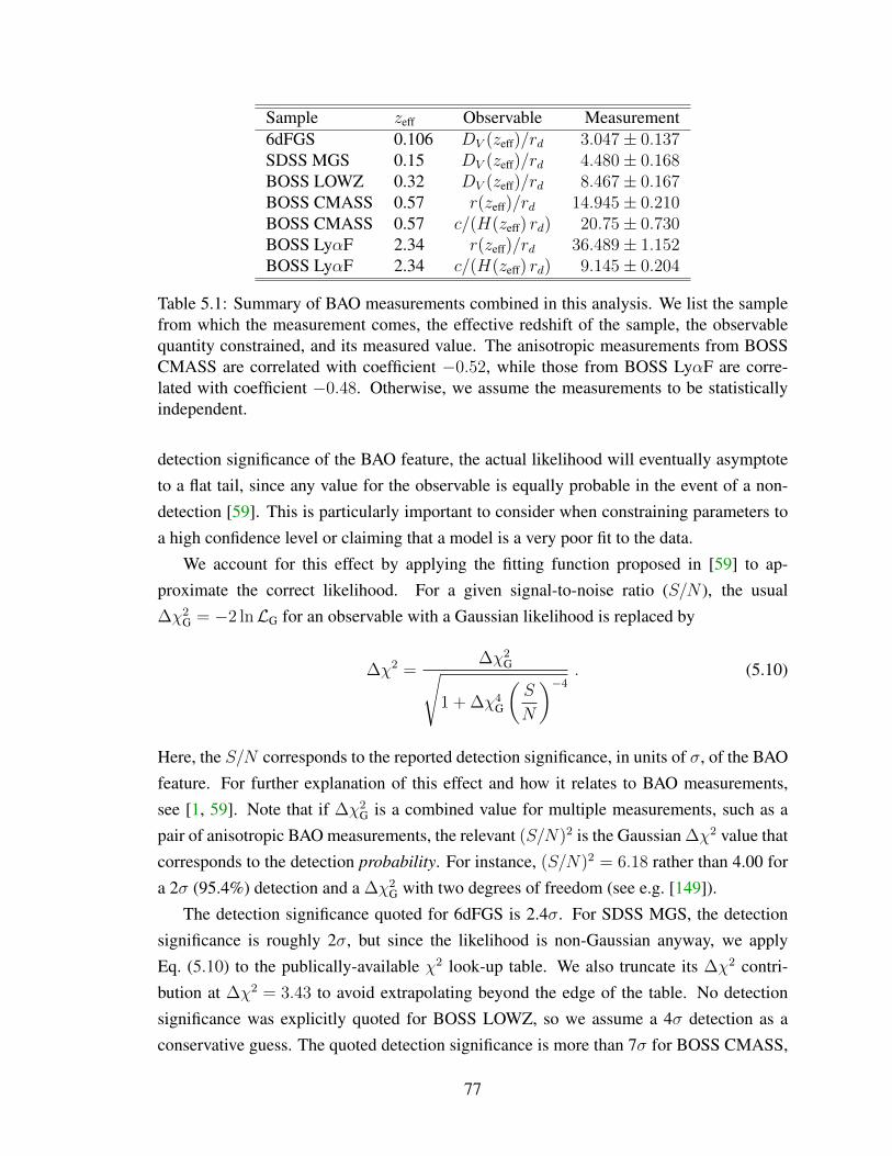
Sample zeff Observable Measurement6dFGS 0.106 DV (zeff)/rd 3.047± 0.137SDSS MGS 0.15 DV (zeff)/rd 4.480± 0.168BOSS LOWZ 0.32 DV (zeff)/rd 8.467± 0.167BOSS CMASS 0.57 r(zeff)/rd 14.945± 0.210BOSS CMASS 0.57 c/(H(zeff) rd) 20.75± 0.730BOSS LyαF 2.34 r(zeff)/rd 36.489± 1.152BOSS LyαF 2.34 c/(H(zeff) rd) 9.145± 0.204

Table 5.1: Summary of BAO measurements combined in this analysis. We list the samplefrom which the measurement comes, the effective redshift of the sample, the observablequantity constrained, and its measured value. The anisotropic measurements from BOSSCMASS are correlated with coefficient −0.52, while those from BOSS LyαF are corre-lated with coefficient −0.48. Otherwise, we assume the measurements to be statisticallyindependent.

detection significance of the BAO feature, the actual likelihood will eventually asymptoteto a flat tail, since any value for the observable is equally probable in the event of a non-detection [59]. This is particularly important to consider when constraining parameters toa high confidence level or claiming that a model is a very poor fit to the data.

We account for this effect by applying the fitting function proposed in [59] to ap-proximate the correct likelihood. For a given signal-to-noise ratio (S/N ), the usual∆χ2

G = −2 lnLG for an observable with a Gaussian likelihood is replaced by

∆χ2 =∆χ2

G√1 + ∆χ4

G

(S

N

)−4. (5.10)

Here, the S/N corresponds to the reported detection significance, in units of σ, of the BAOfeature. For further explanation of this effect and how it relates to BAO measurements,see [1, 59]. Note that if ∆χ2

G is a combined value for multiple measurements, such as apair of anisotropic BAO measurements, the relevant (S/N)2 is the Gaussian ∆χ2 value thatcorresponds to the detection probability. For instance, (S/N)2 = 6.18 rather than 4.00 fora 2σ (95.4%) detection and a ∆χ2

G with two degrees of freedom (see e.g. [149]).The detection significance quoted for 6dFGS is 2.4σ. For SDSS MGS, the detection

significance is roughly 2σ, but since the likelihood is non-Gaussian anyway, we applyEq. (5.10) to the publically-available χ2 look-up table. We also truncate its ∆χ2 contri-bution at ∆χ2 = 3.43 to avoid extrapolating beyond the edge of the table. No detectionsignificance was explicitly quoted for BOSS LOWZ, so we assume a 4σ detection as aconservative guess. The quoted detection significance is more than 7σ for BOSS CMASS,

77

but we use a value of 6σ in the analysis, in case the likelihood becomes non-Gaussian forother reasons at such a high confidence level. Finally, for BOSS LyαF, the detection signif-icance is 5σ for the auto-correlation measurement and roughly 4σ for the cross-correlationmeasurement. Since these measurements are almost completely independent (see [14]), wesimply add their publically-available χ2 tables. Although the combined detection signifi-cance is presumably higher, we apply Eq. (5.10) to the combined χ2 table assuming a sig-nificance of only 4σ. We then truncate the ∆χ2 contribution at ∆χ2 = 15.93 (less than 4σfor two degrees of freedom) to avoid any extrapolation beyond the table. We have verifiedthat the final results are qualitatively insensitive to the exact choices here and quantitativelysensitive to only the LyαF BAO significance, which we discuss in Sec. 5.5.

Measurements of the BAO scale are typically calibrated by the CMB, which effectivelyfixes the sound horizon rd by precisely constraining Ωmh

2 and Ωbh2. Here we avoid using

the CMB to measure the sound horizon, as this measurement is model-dependent. To thisend, we simply allow rd to be a free parameter, effectively using only relative distance in-formation from BAO. This is analogous to SN Ia analysis, where one usually marginalizesover the SN Ia absolute magnitude, using only relative distance information to constraindark energy. The CMB also provides its own precise measurement of the angular diameterdistance to recombination at z∗ ' 1090 that breaks degeneracies among the parameters de-scribing expansion. Here we will also leave out this high-redshift distance measurement;while it can be thought of as just another BAO measurement (i.e. r(z∗)/rd), the interpre-tation is not completely model-independent because the redshift z∗ of the CMB cannot bedetermined without a model. See [147] for further discussion of these different options forcalibrating BAO measurements.

5.4 Methodology

In this section, we review the statistics we use to determine goodness-of-fit and performthe model comparison.

5.4.1 Goodness of fit

To determine if a model is a good fit to the data, we minimize χ2 over the free modelparameters and calculate the probability P (χ2

min, ν) that a greater χ2min could occur due to

chance alone for a fit with ν = N − k degrees of freedom, where N is the total number of

78

measurements and k is the number of free model parameters. This probability is given by

P (χ2, ν) =

Γ

(ν

2,χ2

2

)Γ(ν

2

) , (5.11)

where Γ(s, x) is the upper incomplete gamma function,

Γ(s, x) =

∫ ∞x

ts−1e−tdt , (5.12)

and Γ(s) = Γ(s, 0) is the (complete) gamma function.

5.4.2 Model comparison

We will use three alternative methods for model comparison. Formally, the different statis-tics have different meanings and are valid under different assumptions, so obtaining consis-tent results using different criteria mitigates the possibility that invalid assumptions aboutthe nature of the data will favor one model over another and lead to invalid conclusions.Each of these statistics accounts for the fact that a simpler model (one with fewer free pa-rameters) is preferable to a more complex model if both fit the data similarly well. Notethat they do not require the different models to be nested; while Rh = ct is nested withinpower law cosmology, neither is nested with ΛCDM. For more information about thesestatistics, and for other interesting uses of model comparison in cosmology, see [150–156].

The Akaike information criterion (AIC) [157], which is grounded in information theory,estimates how much more information is lost when describing data with one model overanother. For a best-fit χ2

min and a model with k free parameters, AIC is given by

AIC = χ2min + 2k . (5.13)

This is an asymptotic expression, and a second-order correction term can be added to makethe criterion more accurate for a finite number of observations:

AICc = AIC +2k (k + 1)

N − k − 1. (5.14)

This makes a small difference when the number of data points N is large (e.g. for the SNdata) but a significant difference if N is small (e.g. for the BAO data). Since AICc reducesto AIC in the limit of large N , we use AICc instead of AIC throughout the analysis.

The Bayesian information criterion (BIC) [158] is also an asymptotic expression, and

79

it follows from a Bayesian argument that considers likelihoods in the exponential family ofprobability distributions, which includes the Gaussian distribution and many other commondistributions. BIC selects the model that is a posteriori most probable. It is given by

BIC = χ2min + k ln(N) . (5.15)

BIC typically (though not always) penalizes extra parameters more severely than AIC.The Bayes factor B10 indicates the likelihood of one model relative to another by in-

tegrating both likelihoods over all values of the model parameters, weighting them by thepriors. This statistic is presumably the most robust, as it considers all values, not just thebest-fit values, of the parameters. It naturally penalizes a model with more free parameters,especially if those parameters do not lead to a better fit. In fact, BIC can be considered anapproximation to the logarithm of the Bayes factor. For a set of data D and two differentmodels M0 and M1 that are described, respectively, by sets of parameters θ0 and θ1, theBayes factor indicates the likelihood of M1 relative to M0 and is given by

B10 =

∫Pr(D|θ1,M1) Pr(θ1|M1) dθ1∫Pr(D|θ0,M0) Pr(θ0|M0) dθ0

. (5.16)

For this analysis, we take the prior distributions Pr(θ|M) to be flat, and we assume that thelikelihoods Pr(D|θ,M) are Gaussian (this assumption is implicit in our definitions of AICand BIC, where we write χ2

min in place of the more general −2 ln(Lmax)). We compute thelikelihoods numerically over grids of parameter values. Analytic marginalization overMand ∆M (e.g. Appendix of [2]) leaves at most four parameters over which to grid, makingthis brute-force approach feasible.

5.5 Results

Table 5.2 lists the best-fit values for the model parameters, including the nuisance parame-ters for the SN and BAO data, for each model discussed in Sec. 5.2 and data combinationdiscussed in Sec. 5.3. Table 5.3 shows the results of the model comparison. For each modeland data combination, we list the number of parameters k that were varied, the total numberof data points N , the best-fit χ2

min, the probability P (χ2min, ν) that a greater χ2

min could occurdue to chance alone for degrees of freedom ν = N − k, and the likelihood of the model rel-ative to ΛCDM for the AICc, BIC, and Bayes factor model comparison statistics. We notethat, while statisticians have proposed various scales that give a qualitative interpretation

80

Model Data Ωm n rd ×H0/c α β M ∆MΛCDM JLA (Stat) 0.287 - - 0.140 3.14 24.11 -0.060ΛCDM JLA (Sys) 0.294 - - 0.141 3.10 24.11 -0.070ΛCDM Union2.1 (Stat) 0.278 - - - - 43.16 0.000ΛCDM Union2.1 (Sys) 0.295 - - - - 43.17 0.000ΛCDM BAO 0.285 - 0.0338 - - - -ΛCDM BAO + JLA (Stat) 0.286 - 0.0338 0.140 3.14 24.11 -0.059ΛCDM BAO + JLA (Sys) 0.288 - 0.0338 0.141 3.10 24.11 -0.070ΛCDM BAO + Union2.1 (Stat) 0.282 - 0.0339 - - 43.16 -0.002ΛCDM BAO + Union2.1 (Sys) 0.288 - 0.0338 - - 43.16 0.001Power Law JLA (Stat) - 1.56 - 0.139 3.14 24.14 -0.061Power Law JLA (Sys) - 1.55 - 0.141 3.10 24.13 -0.071Power Law Union2.1 (Stat) - 1.54 - - - 43.20 -0.022Power Law Union2.1 (Sys) - 1.44 - - - 43.20 -0.003Power Law BAO - 0.93 0.0301 - - - -Power Law BAO + JLA (Stat) - 1.52 0.0333 0.139 3.13 24.14 -0.062Power Law BAO + JLA (Sys) - 1.45 0.0331 0.140 3.09 24.14 -0.072Power Law BAO + Union2.1 (Stat) - 1.49 0.0332 - - 43.20 -0.027Power Law BAO + Union2.1 (Sys) - 1.35 0.0326 - - 43.21 -0.007Rh = ct JLA (Stat) - - - 0.131 3.13 24.24 -0.083Rh = ct JLA (Sys) - - - 0.138 3.07 24.23 -0.077Rh = ct Union2.1 (Stat) - - - - - 43.33 -0.115Rh = ct Union2.1 (Sys) - - - - - 43.29 -0.026Rh = ct BAO - - 0.0308 - - - -Rh = ct BAO + JLA (Stat) - - 0.0308 0.131 3.13 24.24 -0.083Rh = ct BAO + JLA (Sys) - - 0.0308 0.138 3.07 24.23 -0.077Rh = ct BAO + Union2.1 (Stat) - - 0.0308 - - 43.33 -0.115Rh = ct BAO + Union2.1 (Sys) - - 0.0308 - - 43.29 -0.026

Table 5.2: Best-fit values of each parameter varied for each model and data combination.

of the numerical results of model comparison statistics (e.g. Jeffreys’ scale for the Bayesfactor), these are obviously rather subjective, so here we simply discuss the results in termsof relative probabilities (e.g. exp(−∆BIC/2)) and let the reader judge their significance.

From Table 5.3, it is clear that ΛCDM is a good fit to all of the SN Ia data. When sys-tematic errors are included, the fit may even be slightly too good, indicating that the errorsmay be overestimated. This would not be surprising, as the SN analyses generally aim to beconservative when estimating the magnitude of systematic errors. A more surprising resultis that ΛCDM is actually not a very good fit to the BAO data. The fit, with a probabilityof 0.052, corresponds to a nearly 2σ discrepancy. This tension has already been noted (e.g.[147]) and is due to the anisotropic LyαF BAO measurements, with the radial measurementc/(H(2.34) rd) too high and the transverse measurement r(2.34)/rd too low for ΛCDM.This is the case regardless of whether Ωm and rd are constrained by CMB observations(e.g. Planck) or by the combined set of BAO measurements, as in this analysis. The similarvalue of Ωm preferred by both SN Ia and BAO data means extra tension will not arise whencombining the data, and so the combined SN + BAO fits are still very good.

81

Mod

elD

ata

kN

χ2 m

inP

(χ2 m

in,ν

)ex

p(−

∆A

ICc/

2)

exp

(−∆

BIC/2

)B

10

ΛC

DM

JLA

(Sta

t)5

740

722.

60.

621

11

ΛC

DM

JLA

(Sys

)5

740

682.

70.

921

11

ΛC

DM

Uni

on2.

1(S

tat)

358

056

2.2

0.66

11

1Λ

CD

MU

nion

2.1

(Sys

)3

580

545.

10.

831

11

ΛC

DM

BA

O2

711

.00.

052

11

1Λ

CD

MB

AO

+JL

A(S

tat)

674

773

3.6

0.57

11

1Λ

CD

MB

AO

+JL

A(S

ys)

674

769

3.8

0.89

11

1Λ

CD

MB

AO

+U

nion

2.1

(Sta

t)4

587

573.

30.

611

11

ΛC

DM

BA

O+

Uni

on2.

1(S

ys)

458

755

6.1

0.78

11

1Po

wer

Law

JLA

(Sta

t)5

740

725.

80.

590.

200.

200.

17Po

wer

Law

JLA

(Sys

)5

740

682.

70.

921.

01.

00.

84Po

wer

Law

Uni

on2.

1(S

tat)

358

056

7.6

0.60

0.06

90.

069

0.05

7Po

wer

Law

Uni

on2.

1(S

ys)

358

054

7.0

0.81

0.39

0.39

0.28

Pow

erL

awB

AO

27

8.8

0.12

3.0

3.0

1.3

Pow

erL

awB

AO

+JL

A(S

tat)

674

774

8.7

0.41

0.00

053

0.00

053

0.00

065

Pow

erL

awB

AO

+JL

A(S

ys)

674

770

5.0

0.82

0.00

370.

0037

0.00

52Po

wer

Law

BA

O+

Uni

on2.

1(S

tat)

458

759

0.1

0.41

0.00

022

0.00

022

0.00

021

Pow

erL

awB

AO

+U

nion

2.1

(Sys

)4

587

567.

90.

670.

0028

0.00

280.

0026

Rh

=ct

JLA

(Sta

t)4

740

855.

80.

0014

3.2×

10−

29

3.2×

10−28

1.0×

10−28

Rh

=ct

JLA

(Sys

)4

740

721.

30.

641.

2×10−

81.

1×10−7

2.0×

10−8

Rh

=ct

Uni

on2.

1(S

tat)

258

065

6.7

0.01

38.

3×10−

21

7.2×

10−20

2.3×

10−20

Rh

=ct

Uni

on2.

1(S

ys)

258

056

5.7

0.63

9.2×

10−

50.

0008

10.

0001

3R

h=ct

BA

O1

718

.30.

0056

0.21

0.06

90.

42R

h=ct

BA

O+

JLA

(Sta

t)5

747

874.

10.

0005

58.

3×10−

31

8.3×

10−30

1.9×

10−30

Rh

=ct

BA

O+

JLA

(Sys

)5

747

739.

60.

523.

1×10−

10

3.0×

10−9

5.1×

10−10

Rh

=ct

BA

O+

Uni

on2.

1(S

tat)

358

767

5.0

0.00

532.

2×10−

22

2.0×

10−21

4.9×

10−22

Rh

=ct

BA

O+

Uni

on2.

1(S

ys)

358

758

4.0

0.49

2.5×

10−

62.

2×10−5

4.1×

10−6

Tabl

e5.

3:R

esul

tsof

the

mod

elco

mpa

riso

n.Fo

rea

chof

the

mod

els

and

data

com

bina

tions

,we

listt

henu

mbe

rof

para

met

ersk

that

wer

eva

ried

,the

tota

lnum

bero

fdat

apo

intsN

,the

best

-fitχ

2 min

,the

prob

abili

tyP

(χ2 m

in,ν

)th

ata

grea

terχ

2 min

coul

doc

curd

ueto

chan

ceal

one

ford

egre

esof

free

domν

=N−k

,and

the

likel

ihoo

dof

the

mod

elre

lativ

eto

ΛC

DM

fort

heA

ICc,

BIC

,and

Bay

esfa

ctor

mod

elco

mpa

riso

nst

atis

tics.

82

z

DV(z)/r d

×(r

d/D

V(z))

ΛCDM

0 0.5 1 1.5 2 2.50.9

1

1.1

1.2

1.3

1.4

Isotropic BAO measurements

ΛCDM (Ωm = 0.338)

Power Law (n = 0.903)

Power Law (n = 1.5)

Figure 5.1: Fits to an isotropic-only version of the BAO data (black points), where we usethe direct isotropic measurement from BOSS CMASS (z = 0.57) and an isotropic mea-surement derived from the LyαF anisotropic measurements (z = 2.34). We show the bestfit to this modified BAO set for ΛCDM with Ωm and rd varied (solid black), power lawcosmology with n and rd varied (solid blue), and power law cosmology with n = 1.5 andonly rd varied (dashed red), where the value n = 1.5 is roughly the value required to fit theSN Ia data.

As we will see below, the uncalibrated galaxy BAO distances (our set without the LyαFBAO) are not effective in distinguishing between the expansion models we consider here.Although the galaxy BAO measurements are more mature and their systematics have beenmore thoroughly studied, there is no obvious reason why we should ignore the LyαF mea-surements. The original analyses [14, 148] investigate some important systematic effects,and they find no substantial evidence that contamination from these systematics is large.They also show that the measurements are generally robust to variations in the fiducialanalysis pipeline. We therefore use the full set of BAO measurements, including the high-redshift LyαF BAO, leaving open the possibility that power law or Rh = ct cosmologyimproves the fit to the anisotropic data.

Interestingly, power law cosmology is about as good a fit to the SN and BAO dataseparately as ΛCDM. If systematic errors in the SN data are ignored, ΛCDM is preferred,

83

but when the systematics are included, the preference for ΛCDM nearly disappears. Herethe AICc and BIC statistics give identical results simply because ΛCDM and power lawcosmology both have one free model parameter. Power law expansion is actually a betterfit to the BAO data, though the model comparison statistics indicate only a mild preferencefor power law expansion. The Bayes factor, which considers the likelihood averaged overthe respective parameter spaces, is particularly indifferent.

The story changes when SN and BAO data are combined, however, and here ΛCDMis strongly favored by the data. As Table 5.2 suggests, the power law exponent preferredby SN data (n ' 1.5) is much higher than that preferred by BAO data (n = 0.93), and thistension means that the combination strongly disfavors power law cosmology relative toΛCDM, even though power law expansion is still a good fit overall. The relative probabilitythat power law cosmology is the “correct” model is at most 0.0052 ' 1/200, which occursfor the Bayes factor when the JLA SN compilation is used with systematic errors includedin the analysis.

One might wonder whether the low power law exponent (n = 0.93) preferred by theBAO data is due to some effect specific to the anisotropic measurements and the extra de-gree of freedom they probe. To investigate this, and to visualize the fit to the BAO data, weplot an isotropic-only version of the BAO data in Fig. 5.1. Here we have used the directisotropic measurement from BOSS DR11 CMASS [13], DV (0.57)/rd = 13.773± 0.134,and an isotropic measurement we derived from the LyαF anisotropic measurements,DV (2.34)/rd = 30.543± 0.570, where we have propagated the errors and accounted fortheir correlation. Note that, while the direct isotropic measurement from CMASS is in ex-cellent agreement with a measurement inferred in this way, the result is approximately validonly if systematic errors in the anisotropic measurements are negligible compared to thestatistical errors. Obviously there is reason to worry that this is not the case for the LyαFBAO, so our fiducial analysis uses the anisotropic measurements directly, as recommendedin the original analyses.

This issue aside, it is clear from Fig. 5.1 that the preference for a low power law ex-ponent is not some artifact of the anisotropic measurements. Here we show fits to theisotropic-only BAO data for both ΛCDM and power law cosmology. Power law cosmol-ogy is a slightly worse fit than in the fiducial analysis, with χ2

min = 7.03 (a probability of0.071 for three degrees of freedom). ΛCDM is a good fit now that the tension from theanisotropic LyαF measurements has effectively canceled, with χ2

min = 1.65 (a probabilityof 0.65 for three degrees of freedom). We also plot a power law model with the exponentfixed to the value n = 1.5, roughly the value required by the SN Ia data, adjusting only thesound horizon rd to give the best fit. Since we have assumed the same detection signifi-

84

cances (6σ for CMASS and 4σ for LyαF) as in the fiducial analysis, it is no surprise that asmaller value for the sound horizon, which raises the model relative to the data, is preferred.Such a model fits the low-redshift BAO data nicely but misses the LyαF measurement com-pletely. Increasing the detection significance of the LyαF measurement would make thisdiscrepancy with the SN Ia data even more significant, and we believe that our choice hereof 4σ (effectively less when using the χ2 table for the anisotropic measurements) for thecombined auto-correlation and cross-correlation measurement is conservative.

Focusing separately on the Rh = ct universe, we find that it is conclusively disfavoredrelative to ΛCDM for all data combinations that include SN Ia data, with at most a relativeprobability of 0.00081 ' 1/1200, which occurs for BIC when the Union2.1 SN compilationis used without BAO data and with systematic errors included. If systematic errors in theSN data are ignored, theRh = ct universe is a poor fit to the data (for JLA, the fit probabilityof 0.0014 corresponds to a > 3σ discrepancy). The Rh = ct universe is also a poor fit tothe BAO data alone and, despite the fact that Rh = ct benefits from having one less freeparameter, ΛCDM is slightly preferred by the model comparison statistics. Note that here,with N very small, we do not expect the BIC result to be valid, and indeed we find that theAICc statistic, with its correction term for finite sample size, is closer to the Bayes factorresult.

Figure 5.2 illustrates the ΛCDM and Rh = ct fits to the JLA SN data, which we havebinned in redshift by averaging the distance moduli with inverse-covariance weights. Thereare two sets of data points because the SN data were standardized separately for each model,withM, ∆M , α, and β optimized to produce the best fit. While ΛCDM is clearly a goodfit with or without systematic errors included, it is apparent by eye that Rh = ct is a poorfit with statistical errors only. While the overall fit looks reasonable when systematic errorsare included, there is a clear trend in the residuals, with nearby SNe too bright and distantSNe too dim.

5.6 Discussion

In this analysis, we have used goodness-of-fit and model comparison statistics to test powerlaw andRh = ct cosmology against ΛCDM. Before we summarize our conclusions, we dis-cuss some arguments made by proponents of the Rh = ct universe [138–140], particularlythose about hidden model dependence in the SN Ia data.

As mentioned in Sec. 5.1, the authors of [138] criticize the analysis of [137], pointingout that the conclusions are based heavily on visual inspection of plots of reconstructeddynamical quantities (e.g. derivatives of the Hubble parameter). While there is nothing

85

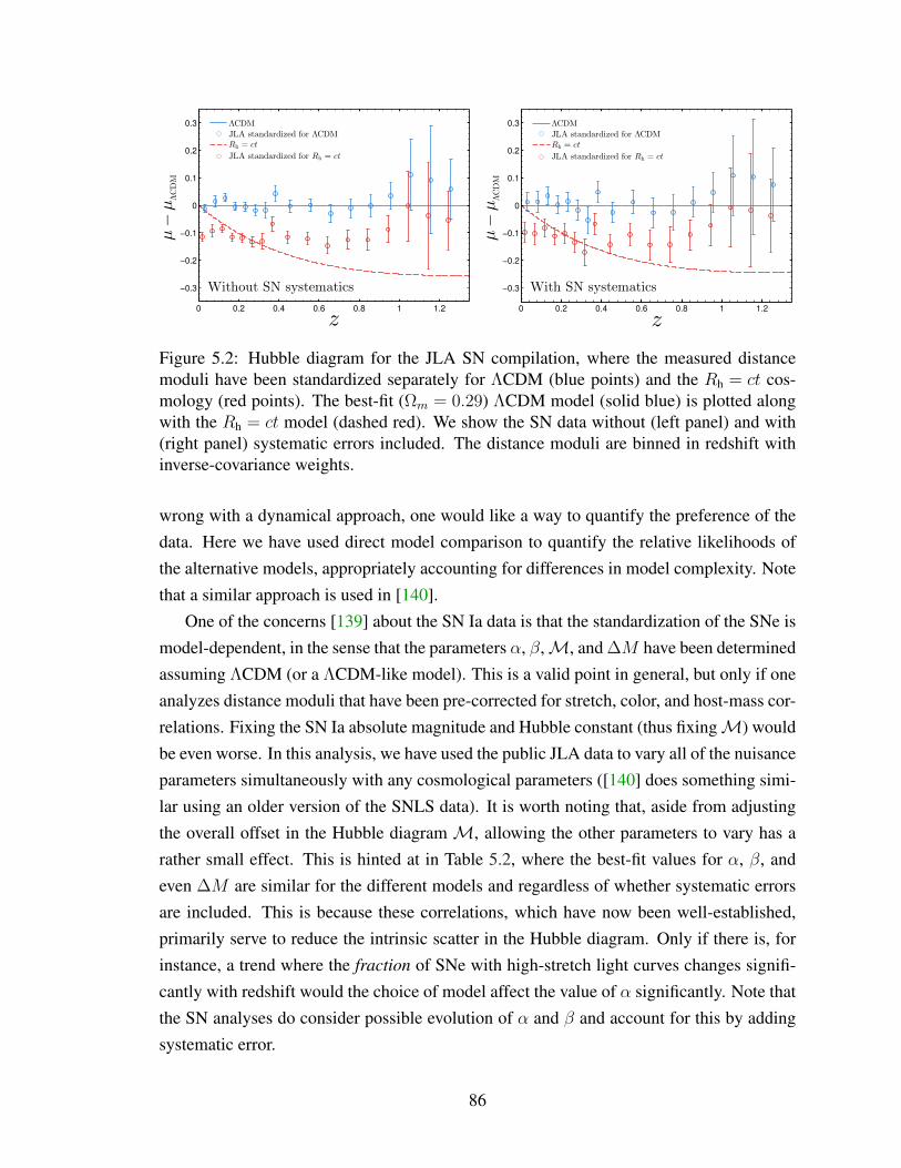
z

µ−µ

ΛCDM

0 0.2 0.4 0.6 0.8 1 1.2

−0.3

−0.2

−0.1

0

0.1

0.2

0.3

z

µ−µ

ΛCDM

0 0.2 0.4 0.6 0.8 1 1.2

−0.3

−0.2

−0.1

0

0.1

0.2

0.3ΛCDM

JLA standardized for ΛCDM

Rh = ct

JLA standardized for Rh = ct

ΛCDM

JLA standardized for ΛCDM

Rh = ct

JLA standardized for Rh = ct

Without SN systematics With SN systematics

Figure 5.2: Hubble diagram for the JLA SN compilation, where the measured distancemoduli have been standardized separately for ΛCDM (blue points) and the Rh = ct cos-mology (red points). The best-fit (Ωm = 0.29) ΛCDM model (solid blue) is plotted alongwith the Rh = ct model (dashed red). We show the SN data without (left panel) and with(right panel) systematic errors included. The distance moduli are binned in redshift withinverse-covariance weights.

wrong with a dynamical approach, one would like a way to quantify the preference of thedata. Here we have used direct model comparison to quantify the relative likelihoods ofthe alternative models, appropriately accounting for differences in model complexity. Notethat a similar approach is used in [140].

One of the concerns [139] about the SN Ia data is that the standardization of the SNe ismodel-dependent, in the sense that the parameters α, β,M, and ∆M have been determinedassuming ΛCDM (or a ΛCDM-like model). This is a valid point in general, but only if oneanalyzes distance moduli that have been pre-corrected for stretch, color, and host-mass cor-relations. Fixing the SN Ia absolute magnitude and Hubble constant (thus fixingM) wouldbe even worse. In this analysis, we have used the public JLA data to vary all of the nuisanceparameters simultaneously with any cosmological parameters ([140] does something simi-lar using an older version of the SNLS data). It is worth noting that, aside from adjustingthe overall offset in the Hubble diagram M, allowing the other parameters to vary has arather small effect. This is hinted at in Table 5.2, where the best-fit values for α, β, andeven ∆M are similar for the different models and regardless of whether systematic errorsare included. This is because these correlations, which have now been well-established,primarily serve to reduce the intrinsic scatter in the Hubble diagram. Only if there is, forinstance, a trend where the fraction of SNe with high-stretch light curves changes signifi-cantly with redshift would the choice of model affect the value of α significantly. Note thatthe SN analyses do consider possible evolution of α and β and account for this by addingsystematic error.

86

The authors of [140] go further and argue that, because the intrinsic scatter is deter-mined by adjusting its value until the reduced χ2 of the fit is equal to one, the intrinsicscatter estimate is model-dependent. This concern is actually addressed in Section 5.5 ofthe JLA analysis [145], which explains that one can avoid this problem by estimating theintrinsic scatter in redshift bins, essentially relying on the fact that the SNe are so constrain-ing, and the redshift coverage so complete, that no parametric model needs to be used atall. In other words, the scatter around the mean in a redshift bin gives the intrinsic scatterfor that bin directly. Although [145] finds an apparent trend where the estimated intrinsicscatter decreases with increasing redshift, the values are consistent with a constant, andultimately a separate value is chosen for each of the four main subsamples, effectivelyallowing for survey-dependent misestimates of other statistical errors. We point out thatthe approach used in [140], where σint is constrained along with the other parameters, re-sults in nearly identical determinations of the intrinsic scatter whether assuming ΛCDM(σint = 0.103± 0.010) or Rh = ct (σint = 0.106± 0.010), indicating that even if the modelmatters in general, it does not in their case.

Why does [140] come to a different conclusion (that Rh = ct is modestly favored overΛCDM) than the present analysis, where similar SN Ia data is used? Presumably the rea-son is that [140] uses only the SNLS SNe, leaving out the low-redshift samples, the mid-redshift SDSS SNe, and the high-redshift SNe from the Hubble Space Telescope, withoutany real justification. This of course removes much of the discriminating power of the SNdata. In Fig. 5.2, notice that only considering the data points in the range 0.4 < z < 1,which roughly corresponds to the redshift range dominated by the SNLS SNe, would makeRh = ct a great fit after the overall height of the data points (M) is adjusted. Even the trendin these residuals (presumably due to their statistical correlation) aligns with the Rh = ct

expansion. While it is true that combining observations of SNe from different instrumentsinto one Hubble diagram is challenging and can lead to concerns about residual systematiceffects, the most important systematic errors (e.g. photometric calibration) are quantifiedin current analyses. For some reason, despite their apparent worry about unaccounted-forsystematic effects, the authors of [140] ignore the known systematic errors altogether, acommon trend in the literature that is usually unjustified and will lead to false conclusions.Here, for instance, systematic errors substantially weaken the model-discriminating powerof the SN data; in fact, it is these systematic errors that allow the Rh = ct universe to be anacceptable overall fit, even if it is conclusively disfavored by the model comparison.

These concerns notwithstanding, we are confident in our conclusions, which we sum-marize as follows. Given the tension in the BAO data resulting from the anisotropic LyαFmeasurements, we find that power law cosmology is a slightly better model than ΛCDM

87

for BAO data alone and is only slightly disfavored relative to ΛCDM for SN Ia data alone.When SN and BAO data are combined, the different power law exponents preferred byeach create substantial tension such that ΛCDM is strongly preferred by the model com-parison statistics (Table 5.3). While the strength of this preference depends on the detectionsignificance of the BOSS LyαF measurement, our choice here (see Sec. 5.3.2) is conser-vative. Also, while the preference for a low power law exponent (n ' 0.9) is due to theLyαF BAO, it is not due to any subtlety in the anisotropic measurements (see Fig. 5.1 andthe discussion in Sec. 5.5). In order to reconcile the power law exponent from BAO withthe higher value (n ' 1.5) required by SN Ia data, an unaccounted-for systematic affectingthe anisotropic LyαF measurements must avoid cancellation in the isotropic measurement,shifting the value by several times its current error. Hopefully, new data (e.g. BOSS DR12)will soon improve these high-redshift BAO measurements, which are clearly important fordistinguishing between alternative models for expansion, including those considered here.

We have also found that the Rh = ct cosmology is nearly ruled out when systematicerrors in the SN Ia data are ignored (for JLA, the fit is unlikely at a level of > 3σ). Withsystematic errors included, the overall fit is acceptable, but ΛCDM is conclusively the bettermodel. The BAO data separately favor ΛCDM, though only slightly, and combining SNand BAO data simply strengthens these conclusions.

88

CHAPTER 6

Peculiar Velocities of SNe Ia

6.1 Introduction

Motions of objects in the universe are not entirely random. Objects which are physicallyclose to one another respond similarly to the pull of large-scale structure, and as a resulttheir peculiar velocities are correlated. Correlations between galaxy peculiar velocitiesare an old subject [159–165], and these velocities have already been used to constraincosmological models, in particular the amount of matter in the universe (see [166] fora review). More recently, peculiar velocities have become important in the analysis oftype Ia supernova (SN Ia) data. At low redshift (z . 0.05), typical peculiar velocities of∼300 km/s are a significant contribution to the SN redshift (for instance, cz = 3,000 km/sat z = 0.01). These peculiar velocities are a nuisance if one is interested in using the SNeto constrain expansion history and dark energy, and it is common practice to propagate thisextra dispersion into the error budget (e.g. add 300 km/s× 5/(cz ln 10) in quadrature to thestatistical uncertainty of each SN magnitude). However, this neglects significant covariancebetween the velocities of different SNe.

Alternatively, one can consider the SN peculiar velocity field itself to be a signal, onethat should contain useful information about the amount and distribution of matter in theuniverse. Nearby SNe are much fewer in number than nearby galaxies, and given thevolume limitation for both, this will likely still be the case in the future. On the other hand,SNe are more useful on a per-object basis because their individual distances can be inferreddirectly and with relative precision — roughly 7% for each SN, depending on the qualityof the observations. Therefore, there has been a resurgence of interest in how SN peculiarvelocities are modeled and used [167, 168].

In this paper, we perform a careful study of the SN velocity correlations in current data,in particular the way in which they are used to draw conclusions about the so-called “bulkvelocity” — the motion, relative to the cosmic microwave background (CMB) rest frame,

89

of the patch of the universe centered on us and containing the nearby sample. Though wefocus on SNe, our methodology is not restricted to SNe and equally applies to analysis ofgalaxy peculiar velocities.

The paper is organized as follows. In section 6.2, we review the physics of how pe-culiar velocities affect SN magnitudes. In section 6.3, we describe the SN samples andhow we use them. In section 6.4, we define a general likelihood that is the basis for ouranalyses, which include a test for the presence of velocity correlations (section 6.5), a testfor the presence of excess bulk velocity beyond that encoded in the correlations predictedin ΛCDM (section 6.6), and a comparison to previous work that studied bulk flows withoutthe velocity covariance (section 6.7). We summarize our conclusions in section 6.8.

6.2 Theoretical framework

6.2.1 Magnification and SN magnitude residuals at low redshifts

The magnitude residuals of standard candles like SNe Ia are directly related to the mag-nification µ, which is defined as the fractional perturbation in the angular diameter andluminosity distances (see [167, 169]),

− 1

2µ =

∆dLdL(z)

=∆dAdA(z)

, (6.1)

where dA(z) and dL(z) denote the background distances evaluated at the observed redshiftz. The second equality, relating luminosity and angular diameter distances, follows fromthe conservation of the photon phase space density. That is, µ describes both the changein the apparent angular size of a spatial ruler as well as the change in observed flux of astandard candle.

Covariant expressions for the magnification at linear order in cosmological perturba-tions have been given in [169–172]. In the conformal-Newtonian (cN) gauge, where themetric is written as

ds2 = a2(τ)[−(1 + 2Ψ) dτ 2 + (1 + 2Φ) δij dx

idxj], (6.2)

90

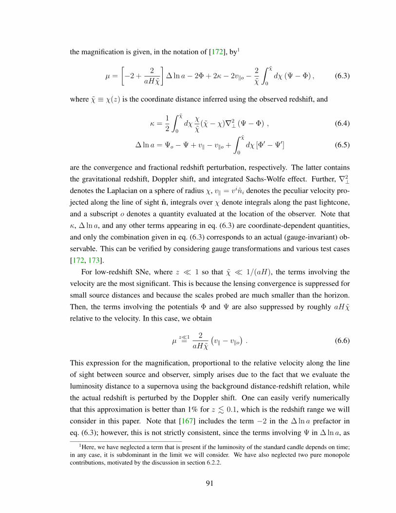
the magnification is given, in the notation of [172], by1

µ =

[−2 +

2

aHχ

]∆ ln a− 2Φ + 2κ− 2v‖o −

2

χ

∫ χ

0

dχ (Ψ− Φ) , (6.3)

where χ ≡ χ(z) is the coordinate distance inferred using the observed redshift, and

κ =1

2

∫ χ

0

dχχ

χ(χ− χ)∇2

⊥ (Ψ− Φ) , (6.4)

∆ ln a = Ψo −Ψ + v‖ − v‖o +

∫ χ

0

dχ [Φ′ −Ψ′] (6.5)

are the convergence and fractional redshift perturbation, respectively. The latter containsthe gravitational redshift, Doppler shift, and integrated Sachs-Wolfe effect. Further, ∇2

⊥

denotes the Laplacian on a sphere of radius χ, v‖ = vini denotes the peculiar velocity pro-jected along the line of sight n, integrals over χ denote integrals along the past lightcone,and a subscript o denotes a quantity evaluated at the location of the observer. Note thatκ, ∆ ln a, and any other terms appearing in eq. (6.3) are coordinate-dependent quantities,and only the combination given in eq. (6.3) corresponds to an actual (gauge-invariant) ob-servable. This can be verified by considering gauge transformations and various test cases[172, 173].

For low-redshift SNe, where z 1 so that χ 1/(aH), the terms involving thevelocity are the most significant. This is because the lensing convergence is suppressed forsmall source distances and because the scales probed are much smaller than the horizon.Then, the terms involving the potentials Φ and Ψ are also suppressed by roughly aHχ

relative to the velocity. In this case, we obtain

µz1=

2

aHχ

(v‖ − v‖o

). (6.6)

This expression for the magnification, proportional to the relative velocity along the lineof sight between source and observer, simply arises due to the fact that we evaluate theluminosity distance to a supernova using the background distance-redshift relation, whilethe actual redshift is perturbed by the Doppler shift. One can easily verify numericallythat this approximation is better than 1% for z . 0.1, which is the redshift range we willconsider in this paper. Note that [167] includes the term −2 in the ∆ ln a prefactor ineq. (6.3); however, this is not strictly consistent, since the terms involving Ψ in ∆ ln a, as

1Here, we have neglected a term that is present if the luminosity of the standard candle depends on time;in any case, it is subdominant in the limit we will consider. We have also neglected two pure monopolecontributions, motivated by the discussion in section 6.2.2.

91

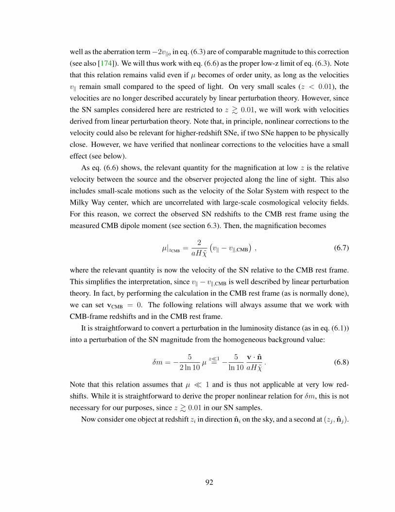
well as the aberration term−2v‖o in eq. (6.3) are of comparable magnitude to this correction(see also [174]). We will thus work with eq. (6.6) as the proper low-z limit of eq. (6.3). Notethat this relation remains valid even if µ becomes of order unity, as long as the velocitiesv‖ remain small compared to the speed of light. On very small scales (z < 0.01), thevelocities are no longer described accurately by linear perturbation theory. However, sincethe SN samples considered here are restricted to z & 0.01, we will work with velocitiesderived from linear perturbation theory. Note that, in principle, nonlinear corrections to thevelocity could also be relevant for higher-redshift SNe, if two SNe happen to be physicallyclose. However, we have verified that nonlinear corrections to the velocities have a smalleffect (see below).

As eq. (6.6) shows, the relevant quantity for the magnification at low z is the relativevelocity between the source and the observer projected along the line of sight. This alsoincludes small-scale motions such as the velocity of the Solar System with respect to theMilky Way center, which are uncorrelated with large-scale cosmological velocity fields.For this reason, we correct the observed SN redshifts to the CMB rest frame using themeasured CMB dipole moment (see section 6.3). Then, the magnification becomes

µ|zCMB =2

aHχ

(v‖ − v‖,CMB

), (6.7)

where the relevant quantity is now the velocity of the SN relative to the CMB rest frame.This simplifies the interpretation, since v‖− v‖,CMB is well described by linear perturbationtheory. In fact, by performing the calculation in the CMB rest frame (as is normally done),we can set vCMB = 0. The following relations will always assume that we work withCMB-frame redshifts and in the CMB rest frame.

It is straightforward to convert a perturbation in the luminosity distance (as in eq. (6.1))into a perturbation of the SN magnitude from the homogeneous background value:

δm = − 5

2 ln 10µz1= − 5

ln 10

v · naHχ

. (6.8)

Note that this relation assumes that µ 1 and is thus not applicable at very low red-shifts. While it is straightforward to derive the proper nonlinear relation for δm, this is notnecessary for our purposes, since z & 0.01 in our SN samples.

Now consider one object at redshift zi in direction ni on the sky, and a second at (zj, nj).

92

We can derive the covariance of their residuals,

Sij ≡ 〈δmi δmj〉 =

[5

ln 10

]2aia′iχi

aja′jχj

ξij

=

[5

ln 10

]2(1 + zi)

2

H(zi)dL(zi)

(1 + zj)2

H(zj)dL(zj)ξij , (6.9)

where ξij is the velocity covariance given by

ξij ≡ ξvelij ≡ 〈(vi · ni)(vj · nj)〉

=dDi

dτ

dDj

dτ

∫dk

2π2P (k, a = 1)

∑`

(2`+ 1)j′`(kχi)j′`(kχj)P`(ni · nj) . (6.10)

Here, primes denote derivatives of the Bessel functions with respect to their arguments,τ is the conformal time, dτ = dt/(a2H), Di is the linear growth function evaluated atredshift zi, and χi = χ(zi). The power spectrum P (k, a) is evaluated in the present (a = 1)and, at the large scales we are interested in, only the first ' 10 terms in the sum over themultipoles contribute. As mentioned above, we use velocities derived from linear theoryand thus insert the linear matter power spectrum for our numerical results. We have verifiedthat using a prescription for the nonlinear matter power spectrum in eq. (6.10) does notsignificantly affect our results. We thus conclude that the linear treatment is sufficient forour purposes. Physically, this is because the dominant contribution to the covariance comesfrom fairly large-scale modes. Note that in our approach, 〈(δmi)

2〉 is assumed to capturethe random motion contribution to the variance of SN residuals.2 While this is not expectedto be completely accurate when using the linear matter power spectrum, the difference inthe diagonal covariance elements is not very significant.3

We have denoted this covariance matrix S to emphasize that this is a cosmologicallyguaranteed “signal” to be added to the “noise” covariance matrix that accounts for thecombination of statistical and systematic errors that affects SN distance measurements,such as intrinsic variations in the SN luminosity (see section 6.3). We again point out thatthe two geometric prefactors in eq. (6.9) each differ by an additive factor of 1 relative tothose in [167] because we drop the term−2 in eq. (6.3) in order to achieve a consistent low-

2An alternative approach by [175] models velocities with perturbation theory based on a density fieldderived from other surveys, and complements them with a “thermal” component of ∼150 km/s added inquadrature to account for nonlinearities. In contrast to our approach, this thus relies on external data sets. Adetailed comparison between the covariances obtained using these different approaches would be interestingbut is beyond the scope of this paper.

3For the low-redshift SNe we consider, nearly all of the redshifts are derived from host galaxy spectra,and so the motion of the SN within its host does not contribute to the residuals.

93

redshift expansion; we have checked that all neglected terms would contribute negligiblyat z . 0.1.

6.2.2 Monopole subtraction

The magnification eq. (6.1) and its low-redshift version eq. (6.6) still have a monopole com-ponent, that is, a contribution that is uniform on the sky. However, since the SN magnituderesiduals are defined with respect to the best-fit distance-redshift relation, this monopoleis mostly absorbed in the fit. While there could technically be a residual monopole signaldue to the fact that our fit (to a flat ΛCDM model, see section 6.4) is very restricted, wewill assume here that the bulk of the monopole is removed. Thus, eq. (6.9) needs to becorrected.

To this end, we define the mean magnitude residual at redshift i as

δm(zi) =

∫δm(zi, n)W (n) d2n , (6.11)

where W (n) is the survey window function, which is normalized such that∫W (n) d2n =

1. Then, noting that we actually measure δmi = δmi − δm(zi), the proper covariance is

Sij ≡⟨δmi δmj

⟩=⟨[δm(zi, ni)− δm(zi)

] [δm(zj, nj)− δm(zj)

]⟩, (6.12)

which can be worked out to be

Sij =

[5

ln 10

]2(1 + zi)

2

H(zi)dL(zi)

(1 + zj)2

H(zj)dL(zj)

dDi

dτ

dDj

dτ

∫dk

2π2P (k, a = 1)

×∑`

(2`+ 1)j′`(kχi)j′`(kχj)

[P`(ni · nj)−

4π

2`+ 1[w`(ni) + w`(nj)] + 4πW`

],

(6.13)

where the survey footprint has been expanded in spherical harmonics,

W (n) =∑`m

w`mY`m(n) , (6.14)

and the coefficients w`(ni) and W` are defined as

w`(n) ≡∑m

w`mY`m(n) , W` ≡∑

m |w`m|22`+ 1

. (6.15)

94

The extra terms in the square brackets in eq. (6.13) are corrections due to the survey win-dow. The W` are therefore just the angular power spectrum (more precisely, the “pseudo-C`”) of the map, while w`(n) is the ` portion of the survey mask at an arbitrary location.Note that, due to the required normalization of W , its value where the survey observes isnot unity, but rather

W (n) =

1

Ωsky(observed sky)

0 (unobserved sky).(6.16)

The term in the square parentheses in the last line of eq. (6.13), which includes thesubtraction of the mean, is therefore a new result that has not, to our knowledge, beenderived and included in previous analyses (although the existence of such a term has beenpointed out in [167, 174]). For a full-sky window, it is easy to show that this term becomesP`(ni · nj) − 1 for ` = 0 and remains equal to the original expression P`(ni · nj) for theother multipoles.

We find that the monopole-subtracted formula leads to small but noticeable changes inthe results, such as the constraints on the parameter A in section 6.5, and we recommendthat it be used in future analyses.

6.3 SN Ia data and noise covariance

For our primary SN Ia dataset, we use the joint light-curve analysis (JLA) [145] of SNefrom the Supernova Legacy Survey (SNLS) and the Sloan Digital Sky Survey (SDSS).JLA includes a recalibration of SNe from the first three years of SNLS [17, 75] along withthe complete SN sample from SDSS, making it the largest combined SN analysis to date.The final compilation includes 740 SNe, ∼100 low-redshift SNe from several subsamples,∼350 from SDSS at low to intermediate redshifts,∼250 from SNLS at intermediate to highredshifts, and ∼10 high-redshift SNe observed with the Hubble Space Telescope.

We combine the individual covariance matrix terms provided4 to compute the full co-variance matrix, which includes statistical errors (correlated uncertainties in the light-curvemeasurements, intrinsic scatter, lensing dispersion) and a variety of systematic errors (pho-tometric calibration, uncertainty in the bias correction, light-curve model uncertainty, po-tential non-Ia contamination, uncertainty in the Milky Way dust extinction correction, anduncertainty in the host galaxy correction).

Although we compute the covariance matrix as described in the JLA analysis, weleave out two contributions to the total error. First, we leave out the additional scatter of

4http://supernovae.in2p3.fr/sdss_snls_jla/

95

150 km/s×5/(cz ln 10) added in quadrature to the other statistical errors on the diagonal toaccount for peculiar velocity. This peculiar velocity scatter does not apply because peculiarvelocities are not a source of noise in our analysis; instead, they are modeled by the formal-ism discussed in section 6.2. We also leave out the systematic error term corresponding touncertainty in the peculiar velocity correction applied to the low-z JLA redshifts. Since ouraim is to study the peculiar velocities themselves, we want to avoid this correction and thenleave out the systematic error associated with it. To this end, we obtain the CMB-frameredshifts zCMB directly from the measured heliocentric redshifts zhel. Specifically, for eachSN we compute

1 + zCMB = (1 + zhel)[1 +

vCMB

c(nCMB · n)

], (6.17)

where n is the sky position of the SN, nCMB is the CMB dipole direction, and vCMB isthe velocity of the Solar System barycenter relative to the CMB rest frame implied by thedipole amplitude. We use the measured values vCMB = 369 km/s and nCMB ≡ (l, b) =

(263.99, 48.26), where the quoted uncertainties [176] are negligible for our purposes.For comparison, we separately consider the Union2 SN Ia analysis [24] from the Super-

nova Cosmology Project.5 We use the full covariance matrix provided for the Union2 SNmagnitudes, but as with JLA, we remove the peculiar velocity scatter (300 km/s here) thatwas added to the diagonal. The redshifts given for the Union2 SNe are just the heliocentricredshifts transformed to the CMB rest frame, so we use them directly.

Note that the Union2 compilation of 557 SNe has been superseded by the Union2.1compilation [25] of 580 SNe, but here the goal is a fair comparison to previous work thatanalyzes the Union2 data. Since the primary change in Union2.1 is the addition of a set ofhigh-redshift SNe, and since only low-redshift SNe are relevant for our analysis, we wouldexpect the two compilations to produce very similar results. When substituting Union2.1for Union2, our results do not change qualitatively, but there are some minor differencesdue to new estimates for some corrected SN magnitudes and their errors. Union2.1 alsoincludes a host-mass correction (see below) that Union2 does not, but this is relativelysmall and only accounts for part of the magnitude differences.

Finally, we briefly consider the low-z compilation from the older analysis of [177],also for comparison with other work. This compilation does not include an analysis ofsystematic errors, so the uncertainty in a SN magnitude is just a combination of the light-curve measurement errors and the derived intrinsic scatter of σint = 0.08 mag. Again,we do not include the peculiar velocity scatter of 300 km/s prescribed for a cosmologicalanalysis. Although CMB-frame redshifts are given, we transform the given heliocentric

5http://supernova.lbl.gov/Union/

96

redshifts into CMB-frame redshifts ourselves using eq. (6.17).Because SNe Ia are not perfect standard candles, it is necessary to correct the observed

peak magnitude of each SN for the empirical correlations between the SN Ia absolute mag-nitude and both the stretch (broadness) and color measure associated with the light-curvefitter. More recently, it has become common to fit for a constant offset in the absolutemagnitude for SNe in high-stellar-mass host galaxies. For JLA, the corrected magnitude istherefore given by

mcorr = m+ α× (stretch)− β × (color) + P ∆M, (6.18)

where α, β, and ∆M are nuisance parameters describing, respectively, the stretch, color,and host-mass corrections. The measured P ≡ P (M∗ > 1010M) is the probability thatthe SN occurred in a high-stellar-mass host galaxy. Note that, as mentioned above, Union2does not include this host-mass correction; also, the analysis of [177] uses a different light-curve fitter with different (but related) light-curve corrections.

For each of the three datasets, we fix the SN Ia nuisance parameters to their best-fitvalues from a fit to the Hubble diagram (for JLA, we perform this fit and correct the magni-tudes ourselves; for the other datasets, we use precorrected magnitudes). In a proper cosmo-logical analysis, one should vary the SN nuisance parameters simultaneously with any cos-mological parameters. In practice, however, the nuisance parameters are well-constrainedby the Hubble diagram with little dependence on the cosmological model, so holding themfixed should be a good approximation, especially for our purposes here.

6.4 Likelihood

We write the full covariance C as the sum of two contributions, C = S + N, where S isthe signal covariance, dominated by velocities at low z and discussed in section 6.2, and N

is the noise covariance, described in section 6.3.Assuming a given cosmological model that allows us to calculate S (eq. (6.9)), the

optimal way to determine whether the data favors peculiar velocities is to consider evidencefor the detection of the full signal matrix S. This approach uses more information in thedata than the search for any particular moment, such as the dipole, of the peculiar velocityfield.

Here we would like to detect evidence for coherent departures of supernova magnitudesfrom the mean — that is, clustering. To do this, we introduce a new dimensionless param-eter A and let S → AS, where A = 1 for the fiducial model. A = 0 corresponds to the

97

case that magnitude residuals are purely due to noise and systematics in the SN Ia data. Wewould like to test whether A is consistent with one and different from zero. Including thenew parameter A, the full covariance becomes

C = AS + N , (6.19)

where 0 ≤ A <∞.On the other hand, allowing for an excess bulk flow component is interesting as well,

as it can be used to search for signatures beyond the fiducial ΛCDM model and also allowsus to compare our results with the existing literature (see section 6.6). In this case, themagnitude residuals are affected by an additional bulk velocity vbulk (e.g. [167]):

∆mbulki ≡ ∆mbulk(vbulk; zi, ni) = −

(5

ln 10

)(1 + zi)

2

H(zi)dL(zi)ni · vbulk , (6.20)

where zi and ni are the redshift and sky position of the SN, while vbulk is a fixed three-dimensional vector. In the quasi-Newtonian picture, vbulk corresponds to the bulk motionof the SN sample; however, in the context of non-standard cosmological models (suchas those breaking homogeneity or isotropy), this should really be seen as a convenientparametrization of the dipole of SN magnitude residuals.

Putting these ingredients together, we construct a multivariate Gaussian likelihood6

L(A,vbulk) ∝1√|C|

exp

[−1

2∆mᵀC−1∆m

], (6.21)

where the elements of the vector ∆m are

(∆m)i = mcorri −mth(zi,M,Ωm)−∆mbulk

i (vbulk) , (6.22)

where mcorri are the observed, corrected magnitudes and mth(zi,M,Ωm) are the theoretical

predictions for the background cosmological model (see below). TheM parameter corre-sponds to the (unknown) absolute calibration of SNe Ia; we analytically marginalize overit in all analyses (e.g. appendix of [2]).

We emphasize that, since the covariance depends on the parameter A that we are inter-ested in constraining, we need to include a term for the 1/

√|C| prefactor in addition to the

6Note that SN flux, or a quantity linearly related to it, might be a better choice for the observable thanthe magnitude, given that we expect the error distribution of the former to be more Gaussian than the latter.Nevertheless, this choice should not impact our results, as the fractional errors in flux are not too large, andwe have explicitly checked that the distribution of the observed magnitudes around the mean is approximatelyGaussian. Therefore we follow most literature on the subject and work directly with magnitudes.

98

100× zCMB

1.1 1.4 1.7 2.2 2.5 3.0 3.5 4.4

100×zCMB

1.1

1.4

1.7

2.2

2.5

3.0

3.5

4.4

-0.04

-0.03

-0.02

-0.01

0

0.01

0.02

0.03

0.04

100× zCMB

1.1 1.4 1.7 2.2 2.5 3.0 3.5 4.4

100×zCMB

1.1

1.4

1.7

2.2

2.5

3.0

3.5

4.4

-0.04

-0.03

-0.02

-0.01

0

0.01

0.02

0.03

0.04

Signal Noise

Figure 6.1: Comparison of the signal (left panel) and noise (right panel) contributions tothe full covariance matrix for the 111 SNe at z < 0.05 from the JLA compilation.

usual χ2 quantity. Since the covariance is a strictly increasing function of A, neglecting theprefactor would lead to the clearly erroneous result that the likelihood is a maximum forA→∞.

The likelihood in eq. (6.21) is the principal tool we will use for our analyses. In thismost general form, the likelihood depends on two input quantities (four parameters, sincethe velocity has three components): the normalization A of the signal component of thecovariance matrix and the excess bulk velocity vbulk not captured by the velocity covariance.Note that, in the fiducial model, A = 1 and vbulk = 0.

Throughout our analyses, we assume a flat ΛCDM model (w = −1, Ωk = 0) with freeparameters fixed to values consistent with data from Planck [178] and other probes. Thatis, we fix Ωm = 0.3, physical matter density Ωmh

2 = 0.14, physical baryon density Ωbh2 =

0.0223, scalar spectral index ns = 0.965, and amplitude of scalar fluctuations As = 2.22×10−9. The corresponding derived value of the Hubble constant is h = 0.683, and that of theamplitude of mass fluctuations is σ8 = 0.79. Within the ΛCDM model, these parametersare determined very precisely using Planck data alone, and we have explicitly checked thatmodest changes in the cosmological model, larger than those allowed by Planck, have anegligible effect on our results. We can therefore conclude that adding Planck priors andmarginalizing over these parameters would not significantly affect our constraints. This isnot surprising. The background cosmology only affects the monopole of the Supernovamagnitudes, and even this dependence is weak at very low redshifts (since we marginalizeoverM). Only a much larger change in the parameters would affect the expected pairwisecovariance, which we do not expect to be able to measure precisely in the first place.

99

In figure 6.1, we compare the noise covariance N to the signal covariance S for ourfiducial cosmology. While the noise contribution is typically larger than the signal, thesignal is not negligible, and it actually dominates for the lowest-redshift SNe. The noise,unlike the signal, becomes effectively smaller as more SNe are used in the analysis, makingthe signal important for the whole redshift range considered (see also the discussion in[179]).

6.5 Constraints on the amplitude of signal covariance

We first consider whether the data itself shows a preference for the presence of the velocity(signal) covariance. Therefore, we explore the constraints on A using the likelihood ineq. (6.21) and fixing vbulk = 0.

The constraints on the parameter A, which determines the fraction of the velocity co-variance added to the full covariance C, are shown in figure 6.2, with the numerical resultsgiven in table 6.1. We have adopted a uniform prior on A such that our Bayesian posterioris proportional to the likelihood in eq. (6.21). All data choices consistently use the availableSNe out to z = 0.05. This leaves 111 objects in the JLA analysis and 132 in the Union2analysis. We have explicitly checked that the results are insensitive to the precise redshiftcutoff; they are driven by the lowest-redshift SNe, and z < 0.05 comfortably captures allof them.

The solid black curve shows JLA, the most current and rigorously calibrated dataset.JLA does not rule out the A = 0 hypothesis; in fact, the likelihood peaks near this value.Nevertheless, JLA is fully consistent with the standard value A = 1, with a probability of0.07 for A > 1.

The solid red curve shows the result from the Union2 dataset. While it is noticeablydifferent than the JLA result, the two likelihoods are mutually consistent; in particular,A = 1 is a satisfactory fit to both. Nevertheless, Union2 is different in that it stronglydisfavors A = 0.

In order to gain additional insight into the difference between the two datasets, we haveidentified SNe at z < 0.05 that overlap between the two datasets, a total of 96 objects.Performing the analysis on this overlap (dashed lines in figure 6.2), we see that the resultsare in better agreement but still somewhat disagree, despite both analyses using the sameSN set. Part of the reason is that JLA and Union2 determine the magnitudes differently;however, even some redshifts do not match. We find a root-mean-square (rms) redshiftdifference of 1.4% for the object-to-object comparison of the 96 overlapping SNe, andthe largest difference is 5%. A further exploration of precisely why the SN redshifts and

100

0 0.5 1 1.5 2 2.5 3A

0

0.2

0.4

0.6

0.8

1

P(A

)

JLAUnion2overlap, JLA 'version'overlap, Union2 'version'

Figure 6.2: Constraints on the parameter A that quantifies the amount of velocity correla-tions (A = 1 is the standard ΛCDM value). The JLA data are consistent with A = 1 butdo not rule out the noise-only hypothesis A = 0. JLA and Union2 give somewhat differentconstraints, though they are not statistically inconsistent. Note that differences remain evenafter restricting to the rather large subset of SNe that they have in common (dashed lines).

magnitudes differ is beyond the scope of this study, but we have explicitly checked that thedifference between JLA and Union2 for the overlap set is largely due to differences in theestimated apparent magnitudes, not the redshifts.7

We also make connection to previous work in [180], where the first cosmological con-straints from the correlations of SN Ia peculiar velocities have been obtained. Instead ofparametrizing the covariance with a multiplicative amplitude, they jointly constrained thecosmological parameters Ωm and σ8. Using the earlier SN dataset from [177], they foundconstraints broadly consistent with ΛCDM values. Using the same dataset, we roughlyagree with [180], our likelihood favoring A ' 1.4 with a large uncertainty but effectivelyruling out A = 0. However, we note that the dataset of [177] includes some SNe withextremely low redshifts (as low as z = 0.002), which are not in the Hubble flow and forwhich the assumption of small residuals in eq. (6.8) breaks down (see also discussion aftereq. (6.10)). Objects at such extremely low redshifts are mutually separated by distances ofa few tens of Mpc; their relative velocities are therefore expected to have important nonlin-

7We have checked that the sky positions of JLA and Union2 overlapping SNe do precisely agree. Wehave also found that the subset of these SNe that are also found in the sample of [177] — 40 in total — haveredshifts that mostly agree very well with JLA, but show larger discrepancies with Union2.

101

ear corrections, in addition to the linear relation eq. (6.8) breaking down, and the analysiswould have to be carefully generalized to take this into account. When we exclude all SNewith z < 0.01 from the dataset of [177], the likelihood for A actually looks very similarto the JLA constraints in figure 6.2, favoring A = 0 but still statistically consistent withA = 1.

To summarize, we find that JLA, the most current and rigorous dataset, does not favorthe presence of SN velocity covariance guaranteed in the ΛCDM model, but is nonethelessconsistent with it. We also find that there is considerable variation in the SN data in termsof their constraints on the velocity covariance, and in particular that the optimistic-lookingresults found in [180] were due to some very-low-redshift SNe that may be too nearby foraccurate modeling with linear theory.

The covariance of SN flux residuals has the potential to provide additional informa-tion about cosmological parameters and other interesting physics [181–185]. Our resultssuggest that current data do not yield interesting constraints. This will likely change withlarger, homogeneous samples with greater sky coverage, such as those expected from theLarge Synoptic Survey Telescope (LSST), currently under construction.

6.6 Constraints on excess bulk velocity

The optimal way to search for the effect of SN velocity correlations in the context of a fidu-cial cosmological model is to test for the presence of the full signal covariance, as we didin section 6.5. However, we can also use the SN magnitude residuals to search for a dipo-lar distortion (for example, due to bulk motion) beyond what is expected in ΛCDM. Thisprovides constraints on physics beyond the concordance cosmology, such as a breaking ofstatistical isotropy or homogeneity, or the presence of a single large long-wavelength per-turbation. The search for bulk flows is the subject of a significant body of literature. Herewe use a different approach, and we make the connection to previous literature in the nextsection.

Bulk velocity is usually defined as the motion of the volume spanned by SNe Ia andthe rest frame defined by the CMB. Moving the SN redshifts to the CMB frame, we arelooking for an overall motion between the SN volume and the rest frame. Since we aimto search for an excess bulk flow beyond ΛCDM, we include the velocity correlations S

in the likelihood, fixing A = 1. Since S includes all velocity correlations within ΛCDM,including the dipole, we expect the posterior for the bulk flow to be consistent with zero ifΛCDM provides a good description of the SN data. Of course, this assumes that our linearmodeling of the velocity correlations is accurate for the SN sample and also that there are

102

-400 -200 0 200 400vbulk [km/s]

0

0.5

1

L(v bu

lk |

n max

-like

)

JLAUnion2JLA, A = 0Union2, A = 0

^

Figure 6.3: A slice through the 3D likelihood for excess bulk velocity. The direction isfixed to be nmax-like (different for each dataset), while the amplitude of the dipole is variedand allowed to be positive or negative. Conclusions about the bulk flow would differ signif-icantly if the velocity signal covariance were set to zero (dashed lines), as in most previouswork on the subject.

no unaccounted-for systematic errors in the SN data that could masquerade as an excessbulk flow.

For this analysis, we therefore adopt the likelihood from eq. (6.21), setting A = 1

but allowing the bulk velocity vbulk = (vbulk, θ, φ) to vary in magnitude and direction. Inorder to get a sense of the three-dimensional likelihood L(vbulk, θ, φ), we first consider thelikelihood of the excess bulk flow amplitude in a cut through the best-fit direction, that is,as a function of vbulk with θ and φ set to their maximum-likelihood values. This is shownin figure 6.3, and note that we continue the scan past zero velocity in the direction oppositethat of the best fit by letting the amplitude of the bulk flow take negative values. Becausethe likelihood is Gaussian, and because vbulk enters the observable magnitude linearly (seeeq. (6.20)), the likelihood of the bulk velocity is also guaranteed to be Gaussian. Therefore,the likelihood ratio between the best-fit (vbulk, θ, φ) and vbulk = 0 immediately translatesinto the confidence at which zero excess bulk velocity is ruled out, assuming uniform priorson each component of the vector vbulk.

Figure 6.3 shows that, once the velocity covariance is properly taken into account, SNdata do not favor any bulk velocity beyond the amount expected in ΛCDM. For example,

103

0 100 200 300 400 500vbulk [km/s]

0

0.5

1

Ang

le-a

vera

ged

P(v

bulk

)

JLAUnion2JLA, A = 0Union2, A = 0

Figure 6.4: Angle-averaged posterior on the amplitude of bulk velocity in excess of thecorrelations captured by the full ΛCDM velocity covariance. Both JLA and Union2 dataare consistent with zero velocity, with relatively large error. The conclusion would againbe very different if the velocity covariance were artificially set to zero (dashed lines).

the JLA likelihood peaks at (vbulk, l, b) = (187 km/s, 323, 25), but this likelihood is largerthan that for vbulk = 0 only by−2∆ lnL = −1.6, far too low even for 68.3% (1σ) evidence,which in three dimensions would be −2∆ lnL ' −3.5.

We would now like to explicitly calculate the posterior distribution of the amplitudeof an excess bulk velocity. Assuming uniform priors on each component of vbulk wouldproduce an additional v2

bulk factor in the posterior, driving it to zero for the vbulk = 0 case sothat vbulk = 0 is automatically ruled out. An alternative that allows us to test the vbulk = 0

assumption, implicitly (or explicitly [186]) adopted by most previous work, is to choosethe prior Pr(vbulk) ∝ 1/v2

bulk or, alternatively, to consider the angle-averaged likelihood

P angle-averaged(vbulk) ∝∫L(vbulk) d cos θ dφ . (6.23)

We plot this likelihood in figure 6.4. It is immediately apparent that both JLA andUnion2 data show no preference for excess bulk velocity, though there is a large uncertainty.Performing the same analysis but setting the velocity correlations to zero (so that C = N

with S = 0), the results are drastically different, favoring bulk flows of several hundredkm/s and, in the case of Union2, firmly ruling out the vbulk = 0 case. This is in agreement

104

with the conclusion found in previous work [187–192]. In the dashed curves shown infigure 6.4, we have not included the 150 km/s (300 km/s) scatter that is added in quadratureto the diagonal of the noise covariance N for JLA (Union2) data in some analyses. Thisclearly does not capture the significant full covariance of SN residuals due to large-scalestructure. However, when adding back this contribution, we find nearly perfect agreementwith the results of [189].

Given the importance of this issue, we stress again that the dashed lines in figures 6.3and 6.4 do not show the proper likelihood of any peculiar velocity, ΛCDM or otherwise,since a guaranteed component of the covariance of the data has been neglected (neverthe-less, one can still use these incorrect likelihoods to construct an estimator for bulk flow,which we will turn to in the next section). Since the velocity covariance S gives a guar-anteed source of correlations in ΛCDM, we argue that it should always be included inlikelihood analyses of SN magnitude residuals. Neglecting this covariance will lead tosuboptimal estimators and, in general, biased results.

6.7 Relation to previous bulk flow measurements

A significant body of earlier work on SN velocities neglected the velocity covariance (andthe lensing covariance, which is important at higher redshifts). These analyses often foundevidence for non-zero bulk flow, and we confirm these findings with our dashed curves infigures 6.3 and 6.4. This bulk velocity with A = 0 is difficult to interpret, since it wasobtained in an analysis with a guaranteed contribution to the covariance of the observablesartificially set to zero.

Nevertheless, one can derive a theoretical expectation for what one should expect forthe bulk velocity derived in this way; we call it vnoise-only

bulk , and in some previous work itcorresponds to what the authors simply call “bulk velocity.” Note that this is not the excess

bulk velocity over the ΛCDM expectation considered in the previous sections.We will adopt the likelihood from eq. (6.21) once more, but we define a new vector x

via ∆mbulk(vbulk) ≡ vbulk x, where

xi ≡ −(

5

ln 10

)(1 + zi)

2

H(zi)dL(zi)ni · nbulk . (6.24)

To estimate vnoise-onlybulk , we set the signal covariance to zero, assume a fixed direction

nbulk, and find the maximum of the likelihood; that is

vnoise-onlybulk ←→ max

vbulk[L(A = 0,vbulk)] . (6.25)

105

Maximizing with respect to vbulk, one finds

vnoise-onlybulk =

yᵀ δm

yᵀ x, (6.26)

where we have defined for convenience a new vector y as y ≡ N−1x, and where δm is thevector of SN magnitude residuals (eq. (6.20) without the ∆mbulk term). Assuming ΛCDM,and still keeping the direction nbulk fixed, the expected (mean) velocity is of course zerosince 〈δmi〉 = 0.

We are more interested in the variance of this quantity, which can be computed directlyand is equal to ⟨(

vnoise-onlybulk

)2⟩

=yᵀ(S + N) y

(yᵀ x)2, (6.27)

since the true SN magnitude covariance for ΛCDM is the sum of both signal and noise:〈(δmi)(δmj)〉 = Sij + Nij . The square root of this quantity is the desired theoreticalexpectation for the rms bulk velocity in ΛCDM when one ignores the signal covariancematrix.

Using the JLA SNe up to redshift z = 0.05, the ΛCDM expectation for the rms ve-locity varies from about 150–170 km/s as a function of nbulk, with a sky-averaged value of162 km/s. Assuming only noise in the data, 〈(δmi)(δmj)〉 = Nij , the result is 71 km/s.The Union2 data give similar results.

We have therefore found that the predicted rms value of vnoise-onlybulk , assuming ΛCDM

and SN data up to z = 0.05, is ∼160 km/s, and that nearly half of this value would begenerated by statistical scatter in SN magnitudes in the absence of any peculiar velocitiesin the universe (such a contribution is sometimes referred to as the “noise bias”). The peakof the JLA likelihood (black dashed line in figure 6.4) is in agreement with the ΛCDMexpectation; Union2 gives a somewhat larger result. Again, however, we caution that theanalysis in this section is suboptimal, given that we do condense the data into a weighteddipole estimator vnoise-only

bulk rather than using the full covariance. Moreover, this estimator issignificantly affected by noise bias which needs to be subtracted. Given the uncertaintiesin the noise covariance, the subtraction of noise bias will lead to additional systematicuncertainties in the actual peculiar velocity measurement.

We have not attempted to repeat the analyses of some past work that studied the velocityfield of low-redshift SNe [190–197] or the anisotropy of the universe from the distributionof nearby SN distances [198–203], since these studies adopted a wide variety of approachesand, in some cases, complicated statistical procedures whose results are calibrated on sim-ulations. We emphasize, however, that the velocity covariance due to large-scale structure

106

P (A) (fig 6.2) vmax-likebulk (fig 6.3) v

angle-avgbulk (fig 6.4)

Survey ML 95% C.L. ∆χ2∣∣A=0

∆χ2∣∣A=1

ML 95% C.L. 95% C.L.

JLA 0.19 (0, 1.15) 0.24 4.13 187 (−108, 485) (0, 376)

Union2 1.19 (0.19, 3.27) 13.2 0.07 265 (−37, 568) (0, 456)

Table 6.1: Summary of numerical results. For both JLA and Union2, we show the best-fit,maximum-likelihood (ML) values and 95% confidence intervals for A. We also show thequantity ∆χ2 (that is, −2∆ lnL) between the best-fit value and special values A = 0 (novelocity signal) and A = 1 (ΛCDM velocity signal). We also show ML and 95% intervalsfor bulk velocity in the best-fit direction and 95% intervals for angle-averaged bulk velocity(here we do not report ML values, which are near zero). All velocities are in units of km/s.

should be included in any such analyses in order to obtain unbiased results and draw reli-able statistical conclusions about the velocity field of the nearby universe.

6.8 Conclusions

In this paper we have revisited the constraints on bulk velocity — the relative motion of thevolume populated by nearby SNe Ia and the rest frame defined by the CMB. Our emphasiswas on a precise and clear procedure for selecting the data, performing the analysis, andmodeling the theoretical expectation. We concentrated on SNe Ia as tracers of cosmicstructure and studied two separate (but overlapping) datasets. Our methodology appliesequally well to galaxies and other tracers of large-scale structure.

We argued, and demonstrated with explicit calculations, that inclusion of the “signal”covariance matrix that captures the peculiar velocity correlations between SNe is crucial.The velocities provide a guaranteed source of covariance between SNe; while the velocitycontribution is subdominant compared to the noise except at the lowest redshifts (see fig-ure 6.1), it does not become smaller as more SNe are included in the analysis. Neglectingthe velocity covariance, as done by a significant body of earlier work on SN velocities andtests of statistical isotropy, leads to results that are both biased and difficult to interpret.

Our approach was based on a likelihood that includes both the signal and noise covari-ance and four free parameters: the normalization A, specifying the fraction of the signaladded to the covariance, and three components of an excess bulk velocity vbulk beyond thatwhich is encoded in the signal covariance. For the fiducial ΛCDM model, A = 1 andvbulk = 0.

We first investigated whether the standard ΛCDM velocity covariance (A = 1) is pre-ferred over the case in which the covariance is ignored (A = 0); that is, we constrained

107

L(A,vbulk = 0). We found that the JLA dataset, while consistent with A = 1, cannot ruleout A = 0, and in fact its likelihood peaks near zero (figure 6.2). Therefore, we did not findconvincing evidence in the data for the correlations expected from velocities. Although weexpect things to change with future data, when precise measurements of a quantity like Awill effectively constrain cosmological parameters such as Ωm and σ8, our results indicatethat current data are not close to providing such useful constraints.

We then pursued a different approach; we assumed a standard ΛCDM velocity covari-ance (theA = 1 case) and tested for excess bulk velocity vbulk beyond that already capturedby the covariance — that is, we adopted the likelihood L(A = 1,vbulk) in the analysis. Wefound that current SN data provide no evidence for a departure from the null hypothesisvbulk = 0 (figures 6.3 and 6.4). This result is in sharp contrast to the inference one wouldhave made by ignoring the velocity covariance (that is, setting A = 0 in the same analysis),as some previous analyses in the literature have done.

To better understand this latter case, we separately studied inferred constraints on a“non-excess” bulk velocity where the velocity covariance has been ignored — that is, theL(A = 0,vnoise-only

bulk ) case. Note that this bulk velocity is more difficult to interpret since itwas obtained by ignoring a guaranteed source of correlations in the data. We showed thatthe rms of the estimated vnoise-only

bulk , assuming ΛCDM and SN data up to z = 0.05, is expectedto be ∼160 km/s, and that nearly half of this value would be generated by a contributionpurely from intrinsic and observational scatter in the SN magnitudes. Therefore, there arereally two problems with this approach: not only is the constrained quantity difficult tointerpret, but it is also guaranteed to be nonzero even without any peculiar velocities in theuniverse, which is clearly not optimal for cosmological interpretations.

The mapping of velocities in the universe using nearby tracers of large-scale structurehas had a remarkably long and productive history. With upcoming large-field, fast-scanningsurveys, it is likely that data will become of sufficiently high quality to enable peculiar ve-locities to progress to the next level and become competitive cosmological probes. Ofcourse, data analysis and theoretical modeling will have to progress as well. In this paperwe have demonstrated that, even for current data, clearly defining the quantities to be con-strained and carefully accounting for the guaranteed correlations between objects due tolarge-scale structure are two factors of key importance.

108

CHAPTER 7

Closing Remarks

Summary

This dissertation investigated systematic effects and performed new cosmological tests withobservational probes of dark energy in anticipation of the precision dark energy constraintsexpected in the near future. Chapters 2–4 studied systematic effects in dark energy probes,focusing on constraints from distance measurements, like those from Type Ia supernovae(SNe Ia). In Chapter 2, we quantified the effect of current SN Ia systematic errors on darkenergy constraints, both for simple parametrizations of the equation of state and for a gen-eral description with principal components. Chapter 3 investigated recent evidence for aphantom equation of state using three separate SN Ia compilations, introducing new teststo search for systematic effects in the data. Chapter 4 was concerned with photometric cal-ibration errors in the galaxy power spectrum. We highlighted the danger of multiplicativeerrors and, using a Fisher matrix formalism, demonstrated a simple way to mitigate theseerrors. Chapters 5–6 focused on tests of the standard cosmological model. In Chapter 5, weused Bayesian model comparison techniques with model-independent SN Ia and BAO datato directly test power law expansion as an alternative cosmological model. In Chapter 6,we used low-redshift SN Ia data to test for the presence of the peculiar velocity correlationspredicted by the standard model. We clarified how these are connected to the bulk velocityof local structure.

As a whole, this body of work demonstrates how the distance probes of dark energy,particularly SNe Ia, can be employed in a variety of ways to test the standard cosmologicalmodel. It also highlights the many subtleties involved in using these probes for precisecosmological measurements, introducing new ways to understand and test for the presenceof systematic effects in the data.

In the coming decade, as we enter an era of big data and of even more precision incosmology, it will be important to reassess the limitations of cosmological probes. Effectsthat were once assumed negligible may become important. With so many different types of

109

data, not to mention the many associated cross-correlations, that one will want to analyzein combination, the question might soon become, which of these many probes are the mostrobust and reliable, rather than which have the best constraining power individually. Fromthis standpoint, there is certainly an important role for the classic, well-studied probes ofdark energy that were the main focus of this dissertation. Below I briefly discuss the futureof these probes, particularly in the context of my own research interests.

CMB

CMB observations are packed with an enormous amount of detailed cosmological infor-mation. But with the exquisitely precise measurements of temperature fluctuations fromPlanck, it is not surprising that we are running into clear signs of tension among variousdata sets. Moderate disagreement with WMAP9 in Planck’s 2013 release was investigatedin [93], and the tension between Planck’s value of H0 (inferred assuming ΛCDM) and thelocal distance-ladder measurements of H0 (e.g. [88], discussed in Sec. 3.3.5) is now well-known in the community. As illustrated nicely in [204], constraints on ΛCDM parametersfrom high multipoles (` > 1000) are in significant tension with those inferred from lowmultipoles (` < 1000), although the latter are now reasonably consistent with WMAP9constraints from that same multipole range as well as with the low-redshift data (e.g. BAO,H0). Further still, Planck SZ cluster counts disagree with those predicted from Planck’sown cosmology, and σ8 inferred from Planck is lower than that inferred from weak lensing(e.g. [205]).

Obviously, sorting out these discrepancies is crucial; if nothing else, hopefully next-generation CMB experiments, which will seek precision polarization measurements at largeand small scales, will help alleviate some of the confusion.

On the other hand, for dark energy research, the CMB distance priors provide mostof the useful information (though CMB lensing is an important exception), and these willcontinue to be crucial for breaking dark energy parameter degeneracies. It is worth studyingdifferent ways to extract this distance information, for instance, whether the observablesdescribed in Sec. 3.2.3 are optimal or whether any such CMB observables are less likelyto be affected by systematics. This latter issue is crucial, since the CMB distance nowtends to dominate combined constraints for simple dark energy descriptions. The modeldependence of the CMB is also an issue, and it would be helpful to understand, in thecontext of the newest CMB observations, which properties of the CMB are robust to variousΛCDM extensions.

110

BAO

Fortuitously, BAO distances are still typically limited by statistical errors (shot noise, cos-mic sampling variance), and measurements of the BAO feature have nicely Gaussian er-rors, at least with the discussion in Sec. 2.4 about treating the tails of the likelihood forlow-signal-to-noise detections notwithstanding. This may change when we aim to pushBAO distance errors to below 1%. A separate question, however, is whether the BAO mea-surements, once they are obtained, indeed function as a standard ruler. Simulations will beneeded here, and unfortunately the answer is probably model-dependent. It may be worthinvestigating other strategies for using the BAO feature (e.g. [206]) that are maximallyreliable and model-independent.

With the newer anisotropic BAO measurements now available (e.g. [13], used in Chap-ter 5), another avenue now exists for testing isotropy and the ΛCDM model. The radial(line-of-sight) and transverse distances should agree, and interestingly, there is already ten-sion here in the higher-redshift LyαF BAO (see Sec. 5.5). In the future, when anisotropicmeasurements exist for many redshift slices, it will be interesting to check whether there isbroad agreement between the radial and transverse correlation functions. Agreement wouldbuild confidence in the robustness of BAO analyses, while disagreement would point to newphysics if confirmed.

SNe Ia

As demonstrated in Chapter 2, SN Ia systematic errors are important even for current data.Of the systematic errors, photometric calibration uncertainty is the most damaging, andit will be the hardest and most important systematic error to control for future surveys.But pushing SN cosmology to its limits is certainly worth it. As a probe, SNe Ia arebasically unique in that each individual SN has the ability to furnish a (nearly) statistically-independent, model-independent, 7% distance measurement.

SN cosmology is very empirical in nature; the stretch and color calibration relations,and the standard candle property itself, are not predicted by any model, at least in prac-tice. There are many ways one could imagine revising or optimizing this modeling. Is itsufficient to model SNe with a single and/or fixed intrinsic scatter (see brief discussion inSec. 5.6)? Is the likelihood for SN observables sufficiently Gaussian? Are fully Bayesiantechniques (e.g. [207, 208]) more appropriate? Should such methods be expanded, or couldthey be simplified? Are there alternative models for SN light-curve corrections that betterexplain the observed data? Can any of the current assumptions be relaxed without losingcosmological information?

111

A precise, direct measurement of H0, independent of the cosmological model and un-correlated with other observations, is a key ingredient for precision dark energy constraints,as it ties relative distances from SNe to the precise distances from CMB and BAO observ-ables. In recent years, various interrelated efforts have been made to characterize the effectof local structure on the H0 measurements and to explain the small but consistent discrep-ancy between direct measurements and the CMB values. As low-redshift SNe (z < 0.1)are used as the last rung of theH0 distance ladder, and SNe in this same range are used sep-arately for cosmology, these measurements may be statistically correlated. On top of this,the peculiar velocity formalism of Chapter 6 is particularly relevant for these low-redshiftSNe, where a sufficiently large sample of SNe essentially becomes a large-scale structuresurvey and should be modeled appropriately.

In light of this, we might ask, to what extent can one use the whole redshift rangeof SNe, not just the lowest-redshift sample, to determine H0, and is this consistent witha purely local measurement? This would empirically test theoretical expectations for theeffect of local structure. Better still, can measurements of Cepheids and other local dis-tance indicators be combined with SNe Ia in a joint cosmological analysis? This wouldtie the local, low-redshift universe to the Hubble expansion in a maximally self-consistentway, effectively adding an H0 measurement but also allowing the peculiar velocities, rel-evant to both H0 and SN cosmology, and the other statistical correlations to be modeledsimultaneously.

112

APPENDIX A

Analytic Marginalization Over Multiple SN IaAbsolute Magnitudes

The computational cost of varying additional nuisance parameters in a likelihood analysiscan be reduced by marginalizing analytically over some of these parameters. The expres-sion for the marginalized χ2 will be more complicated, but fewer likelihoods will need tobe computed in the analysis (in a brute-force grid search, many times fewer). Here we ex-tend Appendix C of [17] and outline a procedure to marginalize analytically over a modelwith more than twoM.

The analytic marginalization over the singleM in Eq. (3.1) is very straightforward. Inthis case, the marginalized χ2 (for a flat prior) is given by

χ2marg = −2 log

∫ ∞−∞

e−χ2/2 dM

= X00 + log

(X11

2π

)− X2

10

X11

, (A.1)

where the unmarginalized χ2 is given by Eq. (3.3) and

X00 = δᵀ C−1δ

X10 = 1ᵀ C−1δ

X11 = 1ᵀ C−11 .

In the above, 1 is a vector of ones and δ is the vector of magnitude residuals without theM term:

δ = ∆m +M1 = mcorr − 5 log10

(H0

cDL

).

Marginalizing over a two-M model is a bit more complicated due to covariance be-tween SNe with differentM. Ignoring this covariance will make things much simpler, but

113

the resulting constraints will be biased and the effect can be significant. For the two-Mcase, we modify Eq. (3.1) so that the vector of predicted SN magnitudes is given by

mth = 5 log10

(H0

cDL

)+M1 x1 +M2 x2 ,

where x1 (x2) is a vector with ones for SNe described byM1 (M2), and zeros otherwise.The marginalized χ2 is given by

χ2marg = X00 + log

(X

4π2

)(A.2)

− 1

X

(X2

10X22 +X220X11 − 2X10X20X12

),

where

X00 = δᵀ C−1δ

X10 = xᵀ1 C−1δ

X20 = xᵀ2 C−1δ

X11 = xᵀ1 C−1x1

X22 = xᵀ2 C−1x2

X12 = xᵀ1 C−1x2

X = X11X22 −X212 .

One can extrapolate the two-M case above to cases with three or more M. This isstraightforward, but the result quickly becomes very messy. Using the familiar result forthe integral of a Gaussian function, one can compute the expression for severalM usingalgebraic manipulation software. Explicit Mathematica code for marginalizing over sixM (as in this work) is given below. The result must be simplified at intermediate steps toavoid long computation times, memory problems, or unmanageable final expressions. Still,the computation below takes several minutes, and the resulting expressions are very long(several pages of small type). This example can easily be modified for more or fewerMand for slightly different parametrizations of the SN magnitude (for instance, treating oneM as a ∆M so that some SNe are described by more than one such nuisance parameter).

114

fexp[a_,b_,c_] := bˆ2/(4*a)+c

fpre[a_,b_,c_] := a/Pi

g[f_,x_] := -1*Coefficient[f,xˆ2],Coefficient[f,x],f/.x->0

pre := 1

exp := -1/2*(X00-2*M1*X10-2*M2*X20-2*M3*X30-2*M4*X40-2*M5*X50-2*M6*X60

+M1ˆ2*X11+M2ˆ2*X22+M3ˆ2*X33+M4ˆ2*X44+M5ˆ2*X55+M6ˆ2*X66

+2*M1*M2*X12+2*M1*M3*X13+2*M1*M4*X14+2*M1*M5*X15+2*M1*M6*X16

+2*M2*M3*X23+2*M2*M4*X24+2*M2*M5*X25+2*M2*M6*X26+2*M3*M4*X34

+2*M3*M5*X35+2*M3*M6*X36+2*M4*M5*X45+2*M4*M6*X46+2*M5*M6*X56)

Do[

coeffs = g[exp,Mi];

pre = FullSimplify[Expand[pre*fpre[coeffs]]];

exp = FullSimplify[Expand[fexp[coeffs]]],Mi,M1,M2,M3,M4,M5,M6]

chisq_marg := Log[pre]-2*exp

115

APPENDIX B

The Biased Angular Power Spectrum

The observed (biased) angular power spectrum for tomographic redshift bins i and j isgiven by

T ij` =

∑m〈ti`mtj∗`m〉2`+ 1

, (B.1)

ti`m =1

1 + εi

ai`m + ci`m +∑`1m1`2m2

R`1 `2 `m1m2m

ci`1m1ai`2m2

−√

4π εi δ`0

, (B.2)

εi =ci00√4π

+1

4π

∑`m

ci`mai∗`m , (B.3)

where the R coupling is defined in Eq. (4.12). Since the monopole of the calibration field(or equivalently, the true mean galaxy density N ) is not measurable, we are free to specifya value, so we choose ci00 = (−1/

√4π)

∑`m c

i`ma

i∗`m so that εi = 0. Then

T ij` =1

2`+ 1

∑m

⟨(ai`m + ci`m) (aj∗`m + cj∗`m)

+∑`1m1`2m2

∑`′1m

′1

`′2m′2

R`1 `2 `m1m2m

R`′1 `

′2 `

m′1m

′2mci`1m1

ai`2m2cj∗`′1m′

1aj∗`′2m′

2(B.4)

+∑`1m1`2m2

R`1 `2 `m1m2m

[(ai`m + ci`m) cj∗`1m1

aj∗`2m2+ (aj∗`m + cj∗`m) ci`1m1

ai`2m2

]⟩

Calculating the ensemble averages, we assume that the cosmological three-point functionvanishes and that the c`m are fixed (not random) variables, with the exception of c00 whichmust be considered separately. Using the definition of Ccal

` in Eq. (4.14), we have (for

116

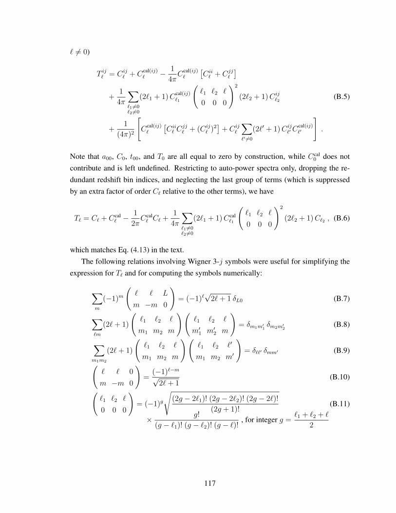
` 6= 0)

T ij` = Cij` + C

cal(ij)` − 1

4πC

cal(ij)`

[Cii` + Cjj

`

]+

1

4π

∑`1 6=0`2 6=0

(2`1 + 1)Ccal(ij)`1

(`1 `2 `

0 0 0

)2

(2`2 + 1)Cij`2

(B.5)

+1

(4π)2

[C

cal(ij)`

[Cii` C

jj` + (Cij

` )2]

+ Cij`

∑`′ 6=0

(2`′ + 1)Cij`′C

cal(ij)`′

].

Note that a00, C0, t00, and T0 are all equal to zero by construction, while Ccal0 does not

contribute and is left undefined. Restricting to auto-power spectra only, dropping the re-dundant redshift bin indices, and neglecting the last group of terms (which is suppressedby an extra factor of order C` relative to the other terms), we have

T` = C` + Ccal` −

1

2πCcal` C` +

1

4π

∑`1 6=0`2 6=0

(2`1 + 1)Ccal`1

(`1 `2 `

0 0 0

)2

(2`2 + 1)C`2 , (B.6)

which matches Eq. (4.13) in the text.The following relations involving Wigner 3-j symbols were useful for simplifying the

expression for T` and for computing the symbols numerically:

∑m

(−1)m

(` ` L

m −m 0

)= (−1)`

√2`+ 1 δL0 (B.7)

∑`m

(2`+ 1)

(`1 `2 `

m1 m2 m

)(`1 `2 `

m′1 m′2 m

)= δm1m′

1δm2m′

2(B.8)

∑m1m2

(2`+ 1)

(`1 `2 `

m1 m2 m

)(`1 `2 `′

m1 m2 m′

)= δ``′ δmm′ (B.9)(

` ` 0

m −m 0

)=

(−1)`−m√2`+ 1

(B.10)(`1 `2 `

0 0 0

)= (−1)g

√(2g − 2`1)! (2g − 2`2)! (2g − 2`)!

(2g + 1)!(B.11)

× g!

(g − `1)! (g − `2)! (g − `)! , for integer g =`1 + `2 + `

2

117

BIBLIOGRAPHY

[1] E. J. Ruiz, D. L. Shafer, D. Huterer, and A. Conley, Phys. Rev. D86, 103004 (2012),arXiv:1207.4781 [astro-ph.CO] .

[2] D. L. Shafer and D. Huterer, Phys. Rev. D89, 063510 (2014), arXiv:1312.1688[astro-ph.CO] .

[3] D. L. Shafer and D. Huterer, Mon. Not. Roy. Astron. Soc. 447, 2961 (2015),arXiv:1410.0035 [astro-ph.CO] .

[4] D. L. Shafer, Phys. Rev. D91, 103516 (2015), arXiv:1502.05416 [astro-ph.CO] .

[5] D. Huterer, D. L. Shafer, and F. Schmidt, JCAP 1512, 033 (2015), arXiv:1509.04708[astro-ph.CO] .

[6] S. Carroll, Spacetime and Geometry: An Introduction to General Relativity(Addison-Wesley, San Francisco, CA, 2003).

[7] P. Ade et al. (Planck Collaboration), Astron.Astrophys. 571, A16 (2014),arXiv:1303.5076 [astro-ph.CO] .

[8] A. G. Riess et al. (Supernova Search Team), Astron.J. 116, 1009 (1998), arXiv:astro-ph/9805201 [astro-ph] .

[9] S. Perlmutter et al. (Supernova Cosmology Project), Astrophys.J. 517, 565 (1999),arXiv:astro-ph/9812133 [astro-ph] .

[10] D. J. Eisenstein et al. (SDSS Collaboration), Astrophys.J. 633, 560 (2005),arXiv:astro-ph/0501171 [astro-ph] .

[11] F. Beutler, C. Blake, M. Colless, D. H. Jones, L. Staveley-Smith, et al.,Mon.Not.Roy.Astron.Soc. 416, 3017 (2011), arXiv:1106.3366 [astro-ph.CO] .

[12] R. Tojeiro, A. J. Ross, A. Burden, L. Samushia, M. Manera, et al.,Mon.Not.Roy.Astron.Soc. 440, 2222 (2014), arXiv:1401.1768 [astro-ph.CO] .

[13] L. Anderson et al. (BOSS Collaboration), Mon.Not.Roy.Astron.Soc. 441, 24 (2014),arXiv:1312.4877 [astro-ph.CO] .

[14] T. Delubac et al. (BOSS Collaboration), Astron.Astrophys. 574, A59 (2015),arXiv:1404.1801 [astro-ph.CO] .

118

[15] J. Frieman, M. Turner, and D. Huterer, Ann.Rev.Astron.Astrophys. 46, 385 (2008),arXiv:0803.0982 [astro-ph] .

[16] D. H. Weinberg, M. J. Mortonson, D. J. Eisenstein, C. Hirata, A. G. Riess, et al.,Phys.Rept. 530, 87 (2013), arXiv:1201.2434 [astro-ph.CO] .

[17] A. Conley et al. (SNLS), Astrophys. J. Suppl. 192, 1 (2011), arXiv:1104.1443 [astro-ph.CO] .

[18] W. M. Wood-Vasey et al. (ESSENCE Collaboration), Astrophys.J. 666, 694 (2007),arXiv:astro-ph/0701041 [astro-ph] .

[19] M. Hicken, W. M. Wood-Vasey, S. Blondin, P. Challis, S. Jha, et al., Astrophys.J.700, 1097 (2009), arXiv:0901.4804 [astro-ph.CO] .

[20] R. Kessler, A. Becker, D. Cinabro, J. Vanderplas, J. A. Frieman, et al., Astro-phys.J.Suppl. 185, 32 (2009), arXiv:0908.4274 [astro-ph.CO] .

[21] M. Sullivan, J. Guy, A. Conley, N. Regnault, P. Astier, et al., Astrophys.J. 737, 102(2011), arXiv:1104.1444 .

[22] T. M. Davis, E. Mortsell, J. Sollerman, A. Becker, S. Blondin, et al., Astrophys.J.666, 716 (2007), arXiv:astro-ph/0701510 [astro-ph] .

[23] D. Rubin, E. Linder, M. Kowalski, G. Aldering, R. Amanullah, et al., Astrophys.J.695, 391 (2009), arXiv:0807.1108 [astro-ph] .

[24] R. Amanullah et al., Astrophys. J. 716, 712 (2010), arXiv:1004.1711 [astro-ph.CO].

[25] N. Suzuki et al., Astrophys. J. 746, 85 (2012), arXiv:1105.3470 [astro-ph.CO] .

[26] M. J. Mortonson, W. Hu, and D. Huterer, Phys. Rev. D81, 063007 (2010),arXiv:0912.3816 .

[27] M. Mortonson, W. Hu, and D. Huterer, Phys. Rev. D82, 063004 (2010).

[28] D. Huterer and A. Cooray, Phys.Rev. D71, 023506 (2005), arXiv:astro-ph/0404062[astro-ph] .

[29] Y. Wang and M. Tegmark, Phys. Rev. D71, 103513 (2005), astro-ph/0501351 .

[30] C. Zunckel and R. Trotta, Mon. Not. Roy. Astron. Soc. 380, 865 (2007), astro-ph/0702695 .

[31] G.-B. Zhao, D. Huterer, and X. Zhang, Phys. Rev. D77, 121302 (2008),arXiv:0712.2277 .

[32] A. Hojjati, L. Pogosian, and G.-B. Zhao, JCAP 1004, 007 (2010), arXiv:0912.4843.

119

[33] E. E. Ishida and R. S. de Souza, Astron.Astrophys. 527, A49 (2011),arXiv:1012.5335 .

[34] A. Shafieloo, A. G. Kim, and E. V. Linder, (2012), arXiv:1204.2272 .

[35] M. Seikel, C. Clarkson, and M. Smith, JCAP 1206, 036 (2012), arXiv:1204.2832 .

[36] G.-B. Zhao, R. G. Crittenden, L. Pogosian, and X. Zhang, (2012), arXiv:1207.3804.

[37] J. Guy et al. (SNLS Collaboration), Astron.Astrophys. 466, 11 (2007), arXiv:astro-ph/0701828 [ASTRO-PH] .

[38] B. C. Kelly, Astrophys.J. 665, 1489 (2007), arXiv:0705.2774 [astro-ph] .

[39] W. J. Percival et al. (SDSS Collaboration), Mon.Not.Roy.Astron.Soc. 401, 2148(2010), arXiv:0907.1660 [astro-ph.CO] .

[40] C. Blake, S. Brough, M. Colless, C. Contreras, W. Couch, et al., (2012),arXiv:1204.3674 .

[41] C. Blake, E. Kazin, F. Beutler, T. Davis, D. Parkinson, et al.,Mon.Not.Roy.Astron.Soc. 418, 1707 (2011), arXiv:1108.2635 [astro-ph.CO].

[42] A. G. Sanchez, C. Scoccola, A. Ross, W. Percival, M. Manera, et al., (2012),arXiv:1203.6616 .

[43] L. Anderson, E. Aubourg, S. Bailey, D. Bizyaev, M. Blanton, et al.,Mon.Not.Roy.Astron.Soc. 427, 3435 (2013), arXiv:1203.6594 [astro-ph.CO] .

[44] J. A. Frieman, D. Huterer, E. V. Linder, and M. S. Turner, Phys.Rev. D67, 083505(2003), arXiv:astro-ph/0208100 [astro-ph] .

[45] E. Komatsu et al. (WMAP), Astrophys. J. Suppl. 192, 18 (2011), arXiv:1001.4538 .

[46] N. Christensen, R. Meyer, L. Knox, and B. Luey, Class. Quant. Grav. 18, 2677(2001), astro-ph/0103134 .

[47] J. Dunkley, M. Bucher, P. G. Ferreira, K. Moodley, and C. Skordis,Mon.Not.Roy.Astron.Soc. 356, 925 (2005), astro-ph/0405462 .

[48] N. Metropolis, A. Rosenbluth, M. Rosenbluth, A. Teller, and E. Teller, J.Chem.Phys.21, 1087 (1953).

[49] W. Hastings, Biometrika 57, 97 (1970).

[50] A. Gelman and D. Rubin, Statistical Science 7, 452 (1992).

[51] A. Lewis and S. Bridle, Phys. Rev. D66, 103511 (2002), astro-ph/0205436 .

120

[52] E. V. Linder, Phys.Rev.Lett. 90, 091301 (2003), arXiv:astro-ph/0208512 [astro-ph] .

[53] D. Huterer and G. Starkman, Phys. Rev. Lett. 90, 031301 (2003), astro-ph/0207517.

[54] M. Chevallier and D. Polarski, Int. J. Mod. Phys. D10, 213 (2001), gr-qc/0009008 .

[55] A. Albrecht et al., (2006), astro-ph/0609591 .

[56] D. Huterer and M. S. Turner, Phys. Rev. D64, 123527 (2001), astro-ph/0012510 .

[57] A. J. Albrecht et al., (2009), arXiv:0901.0721 .

[58] M. J. Mortonson, W. Hu, and D. Huterer, Phys. Rev. D79, 023004 (2009),arXiv:0810.1744 .

[59] B. A. Bassett and N. Afshordi, (2010), arXiv:1005.1664 [astro-ph.CO] .

[60] R. Kessler, B. Bassett, P. Belov, V. Bhatnagar, H. Campbell, et al.,Publ.Astron.Soc.Pac. 122, 1415 (2010), arXiv:1008.1024 .

[61] R. Hlozek, M. Kunz, B. Bassett, M. Smith, J. Newling, et al., Astrophys.J. 752, 79(2012), arXiv:1111.5328 .

[62] A. G. Riess, L.-G. Strolger, S. Casertano, H. C. Ferguson, B. Mobasher, et al., As-trophys.J. 659, 98 (2007), arXiv:astro-ph/0611572 [astro-ph] .

[63] R. A. Knop et al. (Supernova Cosmology Project), Astrophys.J. 598, 102 (2003),arXiv:astro-ph/0309368 [astro-ph] .

[64] P. Astier et al. (SNLS Collaboration), Astron.Astrophys. 447, 31 (2006), arXiv:astro-ph/0510447 [astro-ph] .

[65] W. L. Freedman, C. R. Burns, M. Phillips, P. Wyatt, S. Persson, et al., Astrophys.J.704, 1036 (2009), arXiv:0907.4524 [astro-ph.CO] .

[66] M. Kowalski et al. (Supernova Cosmology Project), Astrophys.J. 686, 749 (2008),arXiv:0804.4142 [astro-ph] .

[67] U. Alam, V. Sahni, and A. A. Starobinsky, JCAP 0702, 011 (2007), arXiv:astro-ph/0612381 [astro-ph] .

[68] S. Nesseris and L. Perivolaropoulos, JCAP 0702, 025 (2007), arXiv:astro-ph/0612653 [astro-ph] .

[69] G.-B. Zhao and X.-m. Zhang, Phys.Rev. D81, 043518 (2010), arXiv:0908.1568[astro-ph.CO] .

[70] A. Rest, D. Scolnic, R. Foley, M. Huber, R. Chornock, et al., (2013),arXiv:1310.3828 [astro-ph.CO] .

121

[71] D. Scolnic, A. Rest, A. Riess, M. Huber, R. Foley, et al., Astrophys.J. 795, 45 (2014),arXiv:1310.3824 [astro-ph.CO] .

[72] C. Cheng and Q.-G. Huang, Phys.Rev. D89, 043003 (2014), arXiv:1306.4091 [astro-ph.CO] .

[73] J.-Q. Xia, H. Li, and X. Zhang, Phys.Rev. D88, 063501 (2013), arXiv:1308.0188[astro-ph.CO] .

[74] A. J. Conley, M. Sullivan, E. Hsiao, J. Guy, P. Astier, et al., (2008), arXiv:0803.3441[astro-ph] .

[75] M. Betoule et al. (SDSS), Astron. Astrophys. 552, A124 (2013), arXiv:1212.4864[astro-ph.CO] .

[76] N. Padmanabhan, X. Xu, D. J. Eisenstein, R. Scalzo, A. J. Cuesta, et al.,Mon.Not.Roy.Astron.Soc. 427, 2132 (2012), arXiv:1202.0090 [astro-ph.CO] .

[77] D. J. Eisenstein and W. Hu, Astrophys.J. 496, 605 (1998), arXiv:astro-ph/9709112[astro-ph] .

[78] G. Hinshaw et al. (WMAP), Astrophys.J.Suppl. 208, 19 (2013), arXiv:1212.5226[astro-ph.CO] .

[79] W. Hu and N. Sugiyama, Astrophys.J. 471, 542 (1996), arXiv:astro-ph/9510117[astro-ph] .

[80] Y. Wang and S. Wang, Phys.Rev. D88, 043522 (2013), arXiv:1304.4514 [astro-ph.CO] .

[81] M. Sullivan et al. (SNLS Collaboration), Mon.Not.Roy.Astron.Soc. 406, 782 (2010),arXiv:1003.5119 [astro-ph.CO] .

[82] R. R. Gupta, C. B. D’Andrea, M. Sako, C. Conroy, M. Smith, et al., Astrophys.J.740, 92 (2011), arXiv:1107.6003 [astro-ph.CO] .

[83] R. Kessler, J. Guy, J. Marriner, M. Betoule, J. Brinkmann, et al., Astrophys.J. 764,48 (2013), arXiv:1209.2482 [astro-ph.CO] .

[84] J. Johansson, D. Thomas, J. Pforr, C. Maraston, R. C. Nichol, et al., (2012),arXiv:1211.1386 [astro-ph.CO] .

[85] M. Childress, G. Aldering, P. Antilogus, C. Aragon, S. Bailey, et al., Astrophys.J.770, 108 (2013), arXiv:1304.4720 [astro-ph.CO] .

[86] S. Wang and Y. Wang, Phys.Rev. D88, 043511 (2013), arXiv:1306.6423 [astro-ph.CO] .

[87] M. Rigault, Y. Copin, G. Aldering, P. Antilogus, C. Aragon, et al., Astron.Astrophys.560, A66 (2013), arXiv:1309.1182 [astro-ph.CO] .

122

[88] A. G. Riess, L. Macri, S. Casertano, H. Lampeitl, H. C. Ferguson, et al., Astrophys.J.730, 119 (2011), arXiv:1103.2976 [astro-ph.CO] .

[89] W. Hu, ASP Conf.Ser. 339, 215 (2005), arXiv:astro-ph/0407158 [astro-ph] .

[90] G. Efstathiou, (2013), arXiv:1311.3461 [astro-ph.CO] .

[91] V. Marra, L. Amendola, I. Sawicki, and W. Valkenburg, Phys.Rev.Lett. 110, 241305(2013), arXiv:1303.3121 [astro-ph.CO] .

[92] E. Macaulay, I. K. Wehus, and H. K. Eriksen, (2013), arXiv:1303.6583 [astro-ph.CO] .

[93] D. N. Spergel, R. Flauger, and R. Hlozek, Phys. Rev. D91, 023518 (2015),arXiv:1312.3313 [astro-ph.CO] .

[94] V. de Lapparent, M. J. Geller, and J. P. Huchra, Astrophys.J. 302, L1 (1986).

[95] S. Maddox, G. Efstathiou, W. Sutherland, and J. Loveday,Mon.Not.Roy.Astron.Soc. 243, 692 (1990).

[96] M. Colless et al. (2DFGRS Collaboration), Mon.Not.Roy.Astron.Soc. 328, 1039(2001), arXiv:astro-ph/0106498 [astro-ph] .

[97] S. Cole et al. (2dFGRS Collaboration), Mon.Not.Roy.Astron.Soc. 362, 505 (2005),arXiv:astro-ph/0501174 [astro-ph] .

[98] D. Parkinson, S. Riemer-Sorensen, C. Blake, G. B. Poole, T. M. Davis, et al.,Phys.Rev. D86, 103518 (2012), arXiv:1210.2130 [astro-ph.CO] .

[99] D. G. York et al. (SDSS Collaboration), Astron.J. 120, 1579 (2000), arXiv:astro-ph/0006396 [astro-ph] .

[100] M. Tegmark et al. (SDSS Collaboration), Astrophys.J. 606, 702 (2004), arXiv:astro-ph/0310725 [astro-ph] .

[101] K. N. Abazajian et al. (SDSS Collaboration), Astrophys.J.Suppl. 182, 543 (2009),arXiv:0812.0649 [astro-ph] .

[102] C. P. Ahn et al. (SDSS Collaboration), Astrophys.J.Suppl. 203, 21 (2012),arXiv:1207.7137 [astro-ph.IM] .

[103] K. S. Dawson et al. (BOSS Collaboration), Astron.J. 145, 10 (2013),arXiv:1208.0022 [astro-ph.CO] .

[104] A. J. Ross, L. Samushia, C. Howlett, W. J. Percival, A. Burden, et al.,Mon.Not.Roy.Astron.Soc., in press (2015), arXiv:1409.3242 [astro-ph.CO] .

[105] T. Abbott et al. (Dark Energy Survey Collaboration), astro-ph/0510346 (2005),arXiv:astro-ph/0510346 [astro-ph] .

123

[106] Z. Ivezic, J. Tyson, R. Allsman, J. Andrew, and R. Angel (LSST Collaboration),0805.2366 (2008), arXiv:0805.2366 [astro-ph] .

[107] R. Laureijs et al. (EUCLID Collaboration), 1110.3193 (2011), arXiv:1110.3193[astro-ph.CO] .

[108] T. Goto, I. Szapudi, and B. R. Granett, Mon.Not.Roy.Astron.Soc. 422, L77 (2012),arXiv:1202.5306 [astro-ph.CO] .

[109] A. R. Pullen and C. M. Hirata, Publications of the Astronomical Society of the Pa-cific, Volume 125, Issue 928, pp. 705-718 (2013), 10.1086/671189, arXiv:1212.4500[astro-ph.CO] .

[110] S. Ho, A. Cuesta, H.-J. Seo, R. de Putter, A. J. Ross, et al., Astrophys.J. 761, 14(2012), arXiv:1201.2137 [astro-ph.CO] .

[111] S. Ho, N. Agarwal, A. D. Myers, R. Lyons, A. Disbrow, et al., 1311.2597 (2013),arXiv:1311.2597 [astro-ph.CO] .

[112] N. Agarwal, S. Ho, and S. Shandera, JCAP 1402, 038 (2014), arXiv:1311.2606[astro-ph.CO] .

[113] T. Giannantonio, A. J. Ross, W. J. Percival, R. Crittenden, D. Bacher, et al.,Phys.Rev. D89, 023511 (2014), arXiv:1303.1349 [astro-ph.CO] .

[114] N. Agarwal, S. Ho, A. D. Myers, H.-J. Seo, A. J. Ross, et al., JCAP 1404, 007(2014), arXiv:1309.2954 [astro-ph.CO] .

[115] A. J. Ross, S. Ho, A. J. Cuesta, R. Tojeiro, W. J. Percival, et al.,Mon.Not.Roy.Astron.Soc. 417, 1350 (2011), arXiv:1105.2320 [astro-ph.CO] .

[116] B. Leistedt, H. V. Peiris, D. J. Mortlock, A. Benoit-Levy, and A. Pontzen,Mon.Not.Roy.Astron.Soc. 435, 1857 (2013), arXiv:1306.0005 [astro-ph.CO] .

[117] B. Leistedt and H. V. Peiris, Mon.Not.Roy.Astron.Soc. 444, 2 (2014),arXiv:1404.6530 [astro-ph.CO] .

[118] D. Huterer, C. E. Cunha, and W. Fang, Mon.Not.Roy.Astron.Soc. 432, 2945 (2013),arXiv:1211.1015 [astro-ph.CO] .

[119] L. Knox, R. Scoccimarro, and S. Dodelson, Phys.Rev.Lett. 81, 2004 (1998),arXiv:astro-ph/9805012 [astro-ph] .

[120] D. Huterer, Phys.Rev. D65, 063001 (2002), arXiv:astro-ph/0106399 [astro-ph] .

[121] A. Lewis, A. Challinor, and A. Lasenby, Astrophys.J. 538, 473 (2000), arXiv:astro-ph/9911177 [astro-ph] .

[122] G. Efstathiou, Mon.Not.Roy.Astron.Soc. 348, 885 (2004), arXiv:astro-ph/0310207[astro-ph] .

124

[123] A. Pontzen and H. V. Peiris, Phys.Rev. D81, 103008 (2010), arXiv:1004.2706 [astro-ph.CO] .

[124] M. Kaplinghat, G. Steigman, I. Tkachev, and T. Walker, Phys.Rev. D59, 043514(1999), arXiv:astro-ph/9805114 [astro-ph] .

[125] M. Kaplinghat, G. Steigman, and T. Walker, Phys.Rev. D61, 103507 (2000),arXiv:astro-ph/9911066 [astro-ph] .

[126] A. Dolgov, Phys.Rev. D55, 5881 (1997), arXiv:astro-ph/9608175 [astro-ph] .

[127] D. Jain, A. Dev, and J. Alcaniz, Class.Quant.Grav. 20, 4485 (2003), arXiv:astro-ph/0302025 [astro-ph] .

[128] G. Sethi, A. Dev, and D. Jain, Phys.Lett. B624, 135 (2005), arXiv:astro-ph/0506255[astro-ph] .

[129] Z.-H. Zhu, M. Hu, J. Alcaniz, and Y.-X. Liu, Astron.Astrophys. 483, 15 (2008),arXiv:0712.3602 [astro-ph] .

[130] A. Dolgov, V. Halenka, and I. Tkachev, JCAP 1410, 047 (2014), arXiv:1406.2445[astro-ph.CO] .

[131] F. Melia and A. Shevchuk, Mon.Not.Roy.Astron.Soc. 419, 2579 (2012),arXiv:1109.5189 [astro-ph.CO] .

[132] A. Dev, M. Sethi, and D. Lohiya, Phys.Lett. B504, 207 (2001), arXiv:astro-ph/0008193 [astro-ph] .

[133] A. Dev, M. Safonova, D. Jain, and D. Lohiya, Phys.Lett. B548, 12 (2002),arXiv:astro-ph/0204150 [astro-ph] .

[134] G. F. Lewis, Mon.Not.Roy.Astron.Soc. 432, 2324 (2013), arXiv:1304.1248 [astro-ph.CO] .

[135] F. Melia, Mon.Not.Roy.Astron.Soc. 446, 1191 (2015), arXiv:1406.4918 [astro-ph.CO] .

[136] G. F. Lewis, Mon.Not.Roy.Astron.Soc.Lett. 431, L25 (2013), arXiv:1301.0305[astro-ph.CO] .

[137] M. Bilicki and M. Seikel, Mon.Not.Roy.Astron.Soc. 425, 1664 (2012),arXiv:1206.5130 [astro-ph.CO] .

[138] F. Melia and R. S. Maier, Mon.Not.Roy.Astron.Soc. 432, 2669 (2013),arXiv:1304.1802 [astro-ph.CO] .

[139] F. Melia, Astron.J. 144, 110 (2012), arXiv:1206.6289 [astro-ph.CO] .

[140] J.-J. Wei, X.-F. Wu, F. Melia, and R. S. Maier, Astron.J. 149, 102 (2015),arXiv:1501.02838 [astro-ph.CO] .

125

[141] M. Moresco, L. Verde, L. Pozzetti, R. Jimenez, and A. Cimatti, JCAP 1207, 053(2012), arXiv:1201.6658 [astro-ph.CO] .

[142] M. Moresco, A. Cimatti, R. Jimenez, L. Pozzetti, G. Zamorani, et al., JCAP 1208,006 (2012), arXiv:1201.3609 [astro-ph.CO] .

[143] J. Mosher, J. Guy, R. Kessler, P. Astier, J. Marriner, et al., Astrophys.J. 793, 16(2014), arXiv:1401.4065 [astro-ph.CO] .

[144] M. Rigault, G. Aldering, M. Kowalski, Y. Copin, P. Antilogus, et al., Astrophys.J.,in press (2015), arXiv:1412.6501 [astro-ph.CO] .

[145] M. Betoule et al. (SDSS), Astron. Astrophys. 568, A22 (2014), arXiv:1401.4064[astro-ph.CO] .

[146] M. Sako et al. (SDSS Collaboration), (2014), arXiv:1401.3317 [astro-ph.CO] .

[147] E. Aubourg, S. Bailey, J. E. Bautista, F. Beutler, V. Bhardwaj, et al., (2014),arXiv:1411.1074 [astro-ph.CO] .

[148] A. Font-Ribera, D. Kirkby, N. Busca, J. Miralda-Escude, N. P. Ross, et al., JCAP1405, 027 (2014), arXiv:1311.1767 .

[149] W. H. Press, S. A. Teukolsky, W. T. Vetterling, and B. P. Flannery, NumericalRecipes: The Art of Scientific Computing, 3rd ed. (Cambridge University Press, NewYork, 2007).

[150] A. R. Liddle, Mon.Not.Roy.Astron.Soc. 351, L49 (2004), arXiv:astro-ph/0401198[astro-ph] .

[151] R. Trotta, Mon.Not.Roy.Astron.Soc. 378, 72 (2007), arXiv:astro-ph/0504022 [astro-ph] .

[152] P. Mukherjee, D. Parkinson, P. S. Corasaniti, A. R. Liddle, and M. Kunz,Mon.Not.Roy.Astron.Soc. 369, 1725 (2006), arXiv:astro-ph/0512484 [astro-ph] .

[153] R. Trotta, Contemp.Phys. 49, 71 (2008), arXiv:0803.4089 [astro-ph] .

[154] L. Verde, S. M. Feeney, D. J. Mortlock, and H. V. Peiris, JCAP 1309, 013 (2013),arXiv:1307.2904 [astro-ph.CO] .

[155] L. Verde, P. Protopapas, and R. Jimenez, Phys.Dark Univ. 2, 166 (2013),arXiv:1306.6766 [astro-ph.CO] .

[156] B. Leistedt, H. V. Peiris, and L. Verde, Phys.Rev.Lett. 113, 041301 (2014),arXiv:1404.5950 [astro-ph.CO] .

[157] H. Akaike, IEEE Transactions on Automatic Control 19, 716 (1974).

[158] G. Schwarz, Annals of Statistics 6, 461 (1978).

126

[159] N. Kaiser, Mon. Not. Roy. Astron. Soc. 231, 149 (1989).

[160] K. M. Gorski, M. Davis, M. A. Strauss, S. D. M. White, and A. Yahil, Astrophys. J.344, 1 (1989).

[161] A. Sandage, G. A. Tammann, and A. Yahil, Astrophys. J. 232, 352 (1979).

[162] A. Nusser and M. Davis, Astrophys. J. 736, 93 (2011), arXiv:1101.1650 [astro-ph.CO] .

[163] E. Macaulay, H. A. Feldman, P. G. Ferreira, A. H. Jaffe, S. Agarwal, M. J. Hudson,and R. Watkins, Mon. Not. Roy. Astron. Soc. 425, 1709 (2012), arXiv:1111.3338[astro-ph.CO] .

[164] E. Branchini, M. Davis, and A. Nusser, Mon. Not. Roy. Astron. Soc. 424, 472(2012), arXiv:1202.5206 [astro-ph.CO] .

[165] M. Feix, A. Nusser, and E. Branchini, JCAP 1409, 019 (2014), arXiv:1405.6710[astro-ph.CO] .

[166] M. A. Strauss and J. A. Willick, Phys. Rept. 261, 271 (1995), arXiv:astro-ph/9502079 [astro-ph] .

[167] L. Hui and P. B. Greene, Phys. Rev. D73, 123526 (2006), arXiv:astro-ph/0512159[astro-ph] .

[168] T. M. Davis et al., Astrophys. J. 741, 67 (2011), arXiv:1012.2912 [astro-ph.CO] .

[169] C. Bonvin, R. Durrer, and M. A. Gasparini, Phys. Rev. D73, 023523 (2006), [Erra-tum: Phys. Rev. D85, 029901 (2012)], arXiv:astro-ph/0511183 [astro-ph] .

[170] A. Challinor and A. Lewis, Phys. Rev. D84, 043516 (2011), arXiv:1105.5292 [astro-ph.CO] .

[171] C. Bonvin and R. Durrer, Phys. Rev. D84, 063505 (2011), arXiv:1105.5280 [astro-ph.CO] .

[172] F. Schmidt and D. Jeong, Phys. Rev. D86, 083527 (2012), arXiv:1204.3625 [astro-ph.CO] .

[173] D. Jeong, F. Schmidt, and C. M. Hirata, Phys. Rev. D85, 023504 (2012),arXiv:1107.5427 [astro-ph.CO] .

[174] N. Kaiser and M. J. Hudson, Mon. Not. Roy. Astron. Soc. 450, 883 (2015),arXiv:1411.6339 [astro-ph.CO] .

[175] J. D. Neill, M. J. Hudson, and A. J. Conley (SNLS), Astrophys. J. 661, L123 (2007),arXiv:0704.1654 [astro-ph] .

[176] G. Hinshaw et al. (WMAP), Astrophys. J. Suppl. 180, 225 (2009), arXiv:0803.0732[astro-ph] .

127

[177] S. Jha, A. G. Riess, and R. P. Kirshner, Astrophys. J. 659, 122 (2007), arXiv:astro-ph/0612666 [astro-ph] .

[178] P. A. R. Ade et al. (Planck), (2015), arXiv:1502.01589 [astro-ph.CO] .

[179] I. Ben-Dayan, R. Durrer, G. Marozzi, and D. J. Schwarz, Phys. Rev. Lett. 112,221301 (2014), arXiv:1401.7973 [astro-ph.CO] .

[180] C. Gordon, K. Land, and A. Slosar, Phys. Rev. Lett. 99, 081301 (2007),arXiv:0705.1718 [astro-ph] .

[181] A. Cooray, D. Holz, and D. Huterer, Astrophys. J. 637, L77 (2006), arXiv:astro-ph/0509579 [astro-ph] .

[182] S. Hannestad, T. Haugboelle, and B. Thomsen, JCAP 0802, 022 (2008),arXiv:0705.0979 [astro-ph] .

[183] A. Abate and O. Lahav, Mon. Not. Roy. Astron. Soc. 389, 47 (2008),arXiv:0805.3160 [astro-ph] .

[184] S. Bhattacharya, A. Kosowsky, J. A. Newman, and A. R. Zentner, Phys. Rev. D83,043004 (2011), arXiv:1008.2560 [astro-ph.CO] .

[185] T. Castro and M. Quartin, Mon. Not. Roy. Astron. Soc. 443, L6 (2014),arXiv:1403.0293 .

[186] Y.-Z. Ma, C. Gordon, and H. A. Feldman, Phys. Rev. D83, 103002 (2011),arXiv:1010.4276 [astro-ph.CO] .

[187] R. Watkins, H. A. Feldman, and M. J. Hudson, Mon. Not. Roy. Astron. Soc. 392,743 (2009), arXiv:0809.4041 [astro-ph] .

[188] J. Colin, R. Mohayaee, S. Sarkar, and A. Shafieloo, Mon. Not. Roy. Astron. Soc.414, 264 (2011), arXiv:1011.6292 [astro-ph.CO] .

[189] D.-C. Dai, W. H. Kinney, and D. Stojkovic, JCAP 1104, 015 (2011),arXiv:1102.0800 [astro-ph.CO] .

[190] S. J. Turnbull, M. J. Hudson, H. A. Feldman, M. Hicken, R. P. Kirshner, andR. Watkins, Mon. Not. Roy. Astron. Soc. 420, 447 (2012), arXiv:1111.0631 [astro-ph.CO] .

[191] U. Feindt et al., Astron. Astrophys. 560, A90 (2013), arXiv:1310.4184 [astro-ph.CO] .

[192] G. J. Mathews, B. Rose, P. Garnavich, D. Yamazaki, and T. Kajino, (2014),arXiv:1412.1529 [astro-ph.CO] .

[193] T. Haugboelle, S. Hannestad, B. Thomsen, J. Fynbo, J. Sollerman, and S. Jha,Astrophys. J. 661, 650 (2007), arXiv:astro-ph/0612137 [astro-ph] .

128

[194] A. Weyant, M. Wood-Vasey, L. Wasserman, and P. Freeman, Astrophys. J. 732, 65(2011), arXiv:1103.1603 [astro-ph.CO] .

[195] Y.-Z. Ma and D. Scott, Mon. Not. Roy. Astron. Soc. 428, 2017 (2013),arXiv:1208.2028 [astro-ph.CO] .

[196] A. Johnson et al., Mon. Not. Roy. Astron. Soc. 444, 3926 (2014), arXiv:1404.3799[astro-ph.CO] .

[197] Y.-Z. Ma and J. Pan, Mon. Not. Roy. Astron. Soc. 437, 1996 (2014),arXiv:1311.6888 [astro-ph.CO] .

[198] D. J. Schwarz and B. Weinhorst, Astron. Astrophys. 474, 717 (2007),arXiv:0706.0165 [astro-ph] .

[199] B. Kalus, D. J. Schwarz, M. Seikel, and A. Wiegand, Astron. Astrophys. 553, A56(2013), arXiv:1212.3691 [astro-ph.CO] .

[200] X. Yang, F. Y. Wang, and Z. Chu, Mon. Not. Roy. Astron. Soc. 437, 1840 (2014),arXiv:1310.5211 [astro-ph.CO] .

[201] S. Appleby, A. Shafieloo, and A. Johnson, Astrophys. J. 801, 76 (2015),arXiv:1410.5562 [astro-ph.CO] .

[202] H.-N. Lin, S. Wang, Z. Chang, and X. Li, (2015), arXiv:1504.03428 [astro-ph.CO].

[203] B. Javanmardi, C. Porciani, P. Kroupa, and J. Pflamm-Altenburg, Astrophys. J. 810,47 (2015), arXiv:1507.07560 [astro-ph.CO] .

[204] G. E. Addison, Y. Huang, D. J. Watts, C. L. Bennett, M. Halpern, G. Hinshaw, andJ. L. Weiland, Astrophys. J. 818, 132 (2016), arXiv:1511.00055 [astro-ph.CO] .

[205] T. D. Kitching, L. Verde, A. F. Heavens, and R. Jimenez, (2016), arXiv:1602.02960[astro-ph.CO] .

[206] S. Anselmi, G. D. Starkman, and R. K. Sheth, Mon. Not. Roy. Astron. Soc. 455,2474 (2016), arXiv:1508.01170 [astro-ph.CO] .

[207] M. C. March, R. Trotta, P. Berkes, G. D. Starkman, and P. M. Vaudrevange, Mon.Not. Roy. Astron. Soc. 418, 2308 (2011), [Mon. Not. Roy. Astron. Soc.418,4(2011)],arXiv:1102.3237 [astro-ph.CO] .

[208] D. Rubin et al. (Supernova Cosmology Project), Astrophys. J. 813, 137 (2015),arXiv:1507.01602 [astro-ph.CO] .

129