Sharma Chakravarthy Information Technology Laboratory ...
15
1 Graph Mining Techniques Subdue Sharma Chakravarthy Information Technology Laboratory Computer Science and Engineering Department The University of Texas at Arlington, Arlington, TX 76009 Email: [email protected] URL: http://itlab.uta.edu/sharma Course URL: http://wweb.uta.edu/faculty/sharmac © Sharma Chakravarthy 1 Acknowledgments Parts of this presentation are based on the work of many of my students, especially Ramji Beera, Ramanathan Balachandran, Srihari Padmanabhan, Subhesh Pradhan (and others) National Science Foundation and other agencies for their support of MavHome, Graph mining and other projects Some slides are borrowed from various sources (web and others) © Sharma Chakravarthy 2 Tutorial Outline Graph Mining Approaches Subdue AGM FSG SQL‐Based Graph Mining HDB‐Subdue DB‐FSG (may be) Graph mining applications Email classification Multilayer Network Analysis Conclusions References © Sharma Chakravarthy 3 Need for Graph Mining Association rule mining, decision trees and others mining approaches mine transactional data Do not make use of any structural information Graph based mining techniques are used for mining data that are structural in nature chemical compounds, complex proteins, VLSI circuits, social networks, … as mapping them to other representations is not possible or will lead to loss of structural information © Sharma Chakravarthy 4
Transcript of Sharma Chakravarthy Information Technology Laboratory ...

1
Graph Mining Techniques Subdue
Sharma ChakravarthyInformation Technology Laboratory
Computer Science and Engineering DepartmentThe University of Texas at Arlington, Arlington, TX 76009
Email: [email protected]: http://itlab.uta.edu/sharma
Course URL: http://wweb.uta.edu/faculty/sharmac
© Sharma Chakravarthy 1
Acknowledgments
Parts of this presentation are based on the work of many of my students, especially Ramji Beera, Ramanathan Balachandran, Srihari Padmanabhan, Subhesh Pradhan (and others)
National Science Foundation and other agencies for their support of MavHome, Graph mining and other projects
Some slides are borrowed from various sources (web and others)
© Sharma Chakravarthy 2
Tutorial Outline Graph Mining Approaches
Subdue
AGM
FSG
SQL‐Based Graph Mining
HDB‐Subdue
DB‐FSG (may be)
Graph mining applications
Email classification
Multilayer Network Analysis
Conclusions
References
© Sharma Chakravarthy 3
Need for Graph Mining
Association rule mining, decision trees and others mining approaches mine transactional data
Do not make use of any structural information
Graph based mining techniques are used for mining data that are structural in nature chemical compounds, complex proteins, VLSI
circuits, social networks, …
as mapping them to other representations is not possible or will lead to loss of structural information
© Sharma Chakravarthy 4

2
Need for Graph Mining Significant work in this area includes Subdue substructure discovery algorithm (Cook &
Holder),
HDB-Subdue (Chakrvarthy, Padmanabhan),
Apriori graph mining (AGM) (Inokuchi, Washio, and Motoda),
the frequent subgraph (FSG) technique (Karypis & Kuramochi), and
gSpan approach (J. Han), also SPIN (Huan, Wang, Prins, and Yang)
PageRank and HITS are also graph based
© Sharma Chakravarthy 5
Application:
To determine which amino acid chain dominates in a particular protein
Protein
Protein represented using Graph
O
N
H
NH
CN
C
COCO
© Sharma Chakravarthy 6
Application Domains
Chemical Reaction chains
CAD Circuit Analysis
Social Networks
Credit Domains
Web analysis
Games (Chess, Tic Tac toe)
Program Source Code analysis
Chinese Character data bases
Geology
Web and social network analysis
© Sharma Chakravarthy 7
Graph Based Data Mining
A Graph representation is an intuitive and an obvious choice for a database that has structural information
Graphs can be used to accurately model and represent scientific data sets. Graphs are suitable for capturing arbitrary relations between the various objects.
Graph based data mining aims at discovering interesting and repetitive patterns within these structural representations of data.
© Sharma Chakravarthy

3
Graph Mining: Mapping
Entities/objects Vertices
Object’s attributes Vertex label
Relations between Edges between verticesobjects
Type of relation edge label
Substructure Connected subgraph
Substructure Set of vertices & edges in
Instance input graph that match graph representation of data
© Sharma Chakravarthy 9
Graph Mining Overview
A substructure is a connected subgraph; need to differentiate between substructures and substructure instances
A connected subgraph is a subgraph of the original graph where there is a path between any two vertices
A subgraph Gs = (Vs, Es) of G = (V, E) is induced if Es contains all the edges of E that connect vertices in Vs
Directed and undirected edges are possible; multiple edges between two nodes need to be accommodated; cycles need to be handled
© Sharma Chakravarthy 10
Graph Mining: Complexity
Enumerating all the substructures of a graph has exponential complexity
Subgraph isomorphism (or subgraph matching) is NP‐complete
However, graph isomorphism although belongs to NP is neither known to be solvable in polynomial time nor NP‐complete
Generating canonical labels is O(|V|!), where V is the number of vertices
All approaches have to deal with the above in order to be able to work on large data sets
Different approaches do it differently; scalability depends on the approach and the use of representation
© Sharma Chakravarthy 11
Subdue
One of the earliest work in Graph based data mining Uses sparse adjacency matrix for graph representation
Substructures are evaluated using a metric called Minimum Description Length principle based on adjacency matrices
Capable of matching two graphs, differing by the number of vertices specified by the threshold parameter, inexactly
Performs hierarchical clustering by compressing the input graph with best substructure in each iteration
© Sharma Chakravarthy 12
4
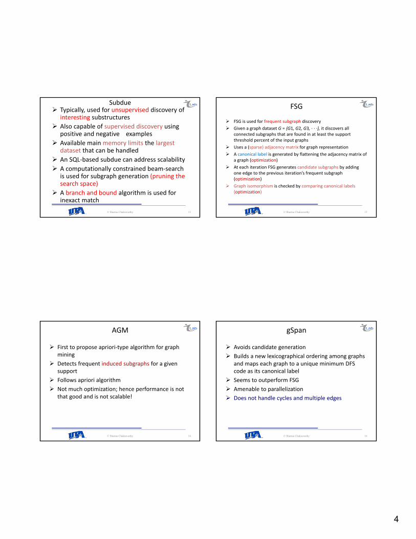
Subdue Typically, used for unsupervised discovery of
interesting substructures
Also capable of supervised discovery using positive and negative examples
Available main memory limits the largest dataset that can be handled
An SQL‐based subdue can address scalability
A computationally constrained beam‐search is used for subgraph generation (pruning the search space)
A branch and bound algorithm is used for inexact match
© Sharma Chakravarthy 13
AGM
First to propose apriori‐type algorithm for graph mining
Detects frequent induced subgraphs for a given support
Follows apriori algorithm
Not much optimization; hence performance is not that good and is not scalable!
© Sharma Chakravarthy 14
FSG
FSG is used for frequent subgraph discovery
Given a graph dataset G = {G1, G2, G3, ∙ ∙ ∙}, it discovers all connected subgraphs that are found in at least the support threshold percent of the input graphs
Uses a (sparse) adjacency matrix for graph representation
A canonical label is generated by flattening the adjacency matrix of a graph (optimization)
At each iteration FSG generates candidate subgraphs by adding one edge to the previous iteration’s frequent subgraph (optimization)
Graph isomorphism is checked by comparing canonical labels (optimization)
© Sharma Chakravarthy 15
gSpan
Avoids candidate generation
Builds a new lexicographical ordering among graphs and maps each graph to a unique minimum DFS code as its canonical label
Seems to outperform FSG
Amenable to parallelization
Does not handle cycles and multiple edges
© Sharma Chakravarthy 16

5
Subdue Example
object
triangle
R1
C1
T1
S1
T2
S2
T3
S3
T4
S4
Input Database Substructure S1(graph form)
Compressed Database
R1
C1
object
squareon
shape
shape S1 S1 S1
S1
• Came from AI• Examples are different from what we normally
see in mining
© Sharma Chakravarthy 17
SUBDUE : Overview
T1
T2 T3
S1
C1
over
shape
shapeobject
object
triangle
square
over
shape
shapeobject
object
triangle
square
overshape
shapeobject
object
triangle
square
object
shape
object
circle
overover
overover
rectangle
shape
Best substructure output by Subdue
Substructure:
Graph(4v,3e):
v 1 object
v 2 object
v 3 triangle
v 4 square
u 1 2 over
u 1 3 shape
u 2 4 shape
© Sharma Chakravarthy 18
Subdue Substructure Discovery System
Subdue Substructure discovery system is a graph‐based data mining system that discovers interesting and repetitive patterns within graph representations of data.
It accepts as input a forest and identifies the substructure that best compresses the input graph using the minimum description length (MDL) principle.
It is capable of identifying both exact and inexact (isomorphic) substructures within a graph
It uses a branch and bound algorithm for inexact matches (substructures that vary slightly in their edge and vertex descriptions).
© Sharma Chakravarthy 19
Subdue
Unsupervised learning Subdue finds the most prevalent substructure from a set of unclassified input graphs
Supervised learning Subdue finds discriminating patterns from a set of classified (positive – G+ and negative – G‐ graphs)
Hierarchical conceptual clustering Compresses G with S and iterate
Incremental Subdue?
© Sharma Chakravarthy 20

6
Subdue
Inferring graph grammars and graph primitives from examples
Applications
Data mining
Pattern recognition
Machine learning
© Sharma Chakravarthy 21
Graph Representation
Subdue represents data as labeled graph. Vertices represent objects or attributes Edges represent relationships between objects Input: Labeled graph Output: Discovered patterns and instances and
their compression value. A substructure is a connected subgraph Graph isomorphism is used to identify similar (not
merely exact) substructures
© Sharma Chakravarthy 22
MDL Principle
Theory to minimize description length (DL) of data (graph)
information theoretic approach
Has been shown to be good across domains
Evaluates substructures based on their ability to compress the DL of a graph
Description length = DL(S) + DL(G/S) Depends upon the representation
Substructure that best compresses the original is chosen
© Sharma Chakravarthy 23
MDL Principle
Best theory: minimizes description length of data
Evaluate substructure based ability to compress DL of graph
Description length = DL(S) + DL(G|S)
© Sharma Chakravarthy 24

7
MDL Principle (cont.) Minimizes description length (MDL) of data
Substructures are evaluated based on their ability to compress the
DL of the entire graph
MDL = description length of the original graph / description length
of the compressed graph
High MDL value is desirable !
DL(G) – Description length of the input graph
DL(S) – Description length of sub graph
DL(G|S) – Description length of the input graph where the sub graph has been substituted
DL(G)MDL =
DL(S) + DL(G|S)
© Sharma Chakravarthy 25
Example: Subdue
© Sharma Chakravarthy 26
Input (partial) The input is a file, with all the vertex labels, vertex
numbers, edges (using vertex numbers) and the edge directions
v 1 A
v 2 B
v 3 C
v 4 D
d 1 2 ab
d 1 3 ac
d 2 4 bd
d 4 3 dc
‘d’ stands for a directed edge and ‘u’ stands for undirected. ‘e’ stands for directed.
© Sharma Chakravarthy 27
Subdue Approach
Create a substructure for each unique vertex
Expand each substructure by adding an edge (and may be a vertex)
Maintain beam number of substructures for expansion
Halting conditions
Discovered substructures > limit
List maintaining the substructures to be expanded becomes empty
Max size of substructure to be discovered is reached
© Sharma Chakravarthy 28

8
Output
Output
Substructure: MDL value = 1.21789, instances = 2
Graph (4v,4e):
v 1 A
v 2 C
v 3 B
v 4 D
d 1 2 ac
d 1 3 ab
d 4 2 dc
d 3 4 bd
© Sharma Chakravarthy 29
Subdue Parameters
Threshold determines the amount of variation permissible in the vertex and edge descriptions during inexact graph match.
Nsubs determines the maximum number of substructures that are returned as the set of best substructures
Beam determines the maximum number of substructures that are retained for expansion in the next iteration of the discovery algorithm
Minsize constrains the size of substructures returned as best to be equal to or more than the specified parameter value
Limit is a upper bound on the number of substructures detected
© Sharma Chakravarthy 30
Subdue AlgorithmSubdue(Graph, BeamWidth, MaxBest, MaxSubSize, Limit)
ParentList = {}; ChildList = {}; BestList = {}
ProcessedSubs = 0
Create a substructure from each unique vertex label and its single‐vertex instances; insert the resulting
substructures in ParentList
while ProcessedSubs <= Limit and ParentList is not empty do
while ParentList is not empty do
Parent = RemoveHead(ParentList)
Extend each instance of Parent in all possible ways; Group the extended instances into Child substructures
foreach Child do
if SizeOf(Child) <= MaxSubSize then
Evaluate the Child //by using MDL
Insert Child in ChildList in order by value //highest to lowest MDL value
if Length(ChildList) > BeamWidth then Destroy the substructure at the end of ChildList
ProcessedSubs = ProcessedSubs + 1
Insert Parent in BestList in order by value
if Length(BestList) > MaxBest then Destroy the substructure at the end of BestList
Switch ParentList and ChildList
return BestList
© Sharma Chakravarthy 31
Algorithm (Contd.)
1. Create substructure for each unique vertex label
circle
rectangle
left
triangle
square
on
on
triangle
square
on
ontriangle
square
on
ontriangle
square
on
onleft
left left
left
Substructures:
triangle (4), square (4),circle (1), rectangle (1)
R1
C1
T1
S1
T2
S2
T3
S3
T4
S4object
triangle
object
squareon
shape
shape
R1
C1
S1 S1 S1
S1
© Sharma Chakravarthy 32

9
Algorithm (Contd.)
2. Expand best substructure by an edge or edge+neighboring vertex
circle
rectangle
left
triangle
square
on
on
triangle
square
on
ontriangle
square
on
ontriangle
square
on
onleft
left left
left
Substructures:
triangle
square
on
circleleftsquare
rectangle
square
on
rectangle
triangleon
R1
C1
T1
S1
T2
S2
T3
S3
T4
S4object
triangle
object
squareon
shape
shape
R1
C1
S1 S1 S1
S1
© Sharma Chakravarthy 33
Algorithm (cont.)
3. Keep only best substructures on queue (specified by beam width)
4. Terminate when queue is empty or #discovered substructures >= limit
5. Compress graph and repeat to generate hierarchical description
6. Constrained to run in polynomial time
R1
C1
T1
S1
T2
S2
T3
S3
T4
S4object
triangle
object
squareon
shape
shape
R1
C1
S1 S1 S1
S1
© Sharma Chakravarthy 34
Graph Match
Exact Graph match
Inexact Graph match
Exact graph match is likely to be restrictive for real life applications.
© Sharma Chakravarthy 35
Inexact Graph Match
Some variations may occur between instances
Want to abstract over minor differences
Difference = cost of transforming one graph to make it isomorphic to another
Match if cost/size < threshold
© Sharma Chakravarthy 36

10
Inexact Graph Match
Minimum graph edit distance
cumulative cost of graph changes required to transform the first graph into a graph isomorphic to the second graph.
Uses Branch and bound algorithm
© Sharma Chakravarthy 37
Variants of Subdue
Hierarchical reduction
Concept learner using positive and negative examples
Similarity detection in social networks
Inductive learning
Partitioned and parallel approaches
Database approach to some of the above
© Sharma Chakravarthy 38
Hierarchical Reduction Input is a labeled graph
A substructure is connected subgraph
A substructure instance is a subgraph isomorphic to substructure definition
Multiple iterations can create hierarchy
S1
S1
S1
S1
S1
S2
S2
S2
© Sharma Chakravarthy 39
Supervised Concept Learning Using Subdue
Need for non‐logic‐based relational concept learner
SubdueCL
Accept positive and negative graphs as input examples
Find hypotheses that describes positive examples and not negative examples
© Sharma Chakravarthy 40

11
SubdueCL
Find substructure compressing positive graphs, but not negative graphs
Find substructure covering positive graphs, but not negative graphs
Learn multiple rules
© Sharma Chakravarthy 41
Concept Learning Subdue
Positive graph G+, Negative graph G‐
Find substructure that compresses positive instances but not (or more than) negative instances
Value (G+, G‐, S) = DL(S) + DL(G+|S) + DL(G‐) – DL(G‐|S)
One of the limitations of this compression‐based concept learner is that it only looks for substructures which compress the entire positive graph more than the entire negative graph.
Therefore, it is biased to look for a substructure that offers more compression as compared to a substructure that covers a greater number of positive examples.
© Sharma Chakravarthy 42
Concept Learning SUBDUE Positive graph G+
Negative graph G‐ Concept:
Alternative set covering measure
Error (substructure) = #PosExNotCovered + #NegExCovered
#PosEx + #NegEx
For a substructure to be good, Error should be minimum
Hence, Value (of a substructure) = 1 – Error
Coverage: A substructure covers an example if the substructure matches a subgraph of the example
© Sharma Chakravarthy 43
Hypotheses detection using coverageMain(Gp, Gn, Beam, Limit)
H = {};
repeat
repeat
BestSub = SubdueCL(Gp, Gn, Beam, Limit)
if BestSub = {}
then Beam m= Beam * 1.1
until (BestSub <> {})
Gp = Gp ‐ {p in Gp | BestSub covers p}
H = H + BestSub
until Gp = {}
return H
end
© Sharma Chakravarthy 44

12
SubdueCL Algorithm
SubdueCL(Gp, Gn, Limit, Beam)
ParentList = (All substructures of one vertex in Gp) mod Beam
repeat
BestList = {}
Exhausted = TRUE
i = Limit
while ( (i > 0 ) and (ParentList ≠ {}) )
ChildList = {}
foreach substucture in ParentList
C = Expand(Substructure)
if CoversOnePos(C,Gp)
then BestList = BestList ∪ {C}
ChildList = ( ChildList ∪ C ) mod Beam
i = i – 1
endfor
ParentList = ChildList mod Beam
endwhile
if BestList = {} and ParentList ≠ {}
then Exhausted = FALSE
Limit = Limit * 1.2
until ( Exhausted = TRUE )
return first(BestList)
end
© Sharma Chakravarthy 45
Example
object
object
object
on
on
triangle
square
shape
shape
© Sharma Chakravarthy 46
Empirical Results
Comparison with ILP (inductive logic programming) systems
Non‐relational domains from UCI repository
Subdue has also been extended for multiple classes
Golf Vote Diabetes Credit TicTacToe
FOIL 66.67 93.02 70.66 66.16 100.00
Progol 33.33 76.98 51.97 44.55 100.00
SubdueCL 66.67 94.88 64.21 71.52 100.00
© Sharma Chakravarthy 47
Graph‐based Anomaly Detection [KDD03] Anomalous substructure detection
Examine entire graph
Report unusual (low MDL compression) substructures
− low count
− lower MDL
− lower compression in subsequent passes
size * count can be used as a heuristic
© Sharma Chakravarthy 48

13
Graph‐based Anomaly Detection [KDD03] Anomalous subgraph detection
Partition graph into distinct, separate structures (subgraphs)
Determine how anomalous each subgraph is compared to others− How early compressed?
− How much compression?
© Sharma Chakravarthy 49
FSG
Aims at discovering interesting sub‐graph(s) thatappear frequently over the entire set of graphs incontrast to discovering a interesting sub‐graph(s)that appear within a single graph (or a forest) as inSubdue/HDB‐Subdue
It is designed along the lines of Apriori algorithm.
© Sharma Chakravarthy 50
Problem Definition
discovering all connected subgraphs that occurfrequently over the entire set of graphs.
Subdue: best n are output (n is user defined)
vertex : corresponds to an entity
edge : correspond to a relation between two entities
© Sharma Chakravarthy 51
Example of Frequent sub-graph discovery
© Sharma Chakravarthy 52

14
Definitions
Gs will be an induced subgraph of G if Vs is a subset of V and Es contains all the edges of E that connect vertices in Vs.
Two graphs G1 = (V1;E1) and G2 = (V2;E2) are isomorphic if they are topologically identical to each other, that is, there is a mapping from V1 to V2 such that each edge in E1 is mapped to a single edge in E2 and vice versa
An automorphism : an isomorphism mapping where G1 = G2 (on the same graph).
© Sharma Chakravarthy 53
Example (from wiki)
Graph G Graph HAn isomorphismbetween G and H
ƒ(a) = 1ƒ(b) = 6ƒ(c) = 8ƒ(d) = 3ƒ(g) = 5ƒ(h) = 2ƒ(i) = 4ƒ(j) = 7
• The two graphs shown below are isomorphic, despite their different looking drawings
• The formal notion of "isomorphism", e.g., of "graph isomorphism", captures the informal notion that some objects have "the same structure" if one ignores individual distinctions of "atomic" components of objects in question
© Sharma Chakravarthy 54
Conclusions
Graph mining is a powerful approach needed by many real‐world applications
There is need for both Subdue class of mining algorithms and frequent subgraph class of algorithms
Scalability is an extremely important issue
Our approach to using SQL has yielded very promising scalability results (800K vertices and 1600K edges)
© Sharma Chakravarthy 55
Subdue FSG AGM gSpan HDBSubdue
Graph Mining
Multiple edges Hierarchical reduction
Cycles
Evaluation metric MDL Frequency Support, Confidence
Frequency DMDL
(frequency)
Inexact graph match
With threshold
Memory limitation
Comparison
© Sharma Chakravarthy 56

15
Scalability Issues
Subdue is a main memory algorithm.
Good performance for small data sizes
Entire graph is constructed before applying the mining algorithm
Takes a very long time to even to initialize for 1600K edges and 800K vertices graph
Scalability is an issue
© Sharma Chakravarthy 57
SQL‐Based Graph Mining
We have mapped the Subdue algorithm using SQL (HDB‐Subdue)
Handles multiple edges between nodes
Handles cycles/loops
Performs Hierarchical reduction
Dveloped DMDL tailored to databases
Can handle graphs of Millions of edges and vertices
DB‐FSG does frequent subgraph mining
Working on inexact matching
© Sharma Chakravarthy 58