
Shape Segmentation -...
85
Shape Segmentation Qixing Huang
-
Upload
truongxuyen -
Category
Documents
-
view
219 -
download
0
Transcript of Shape Segmentation -...
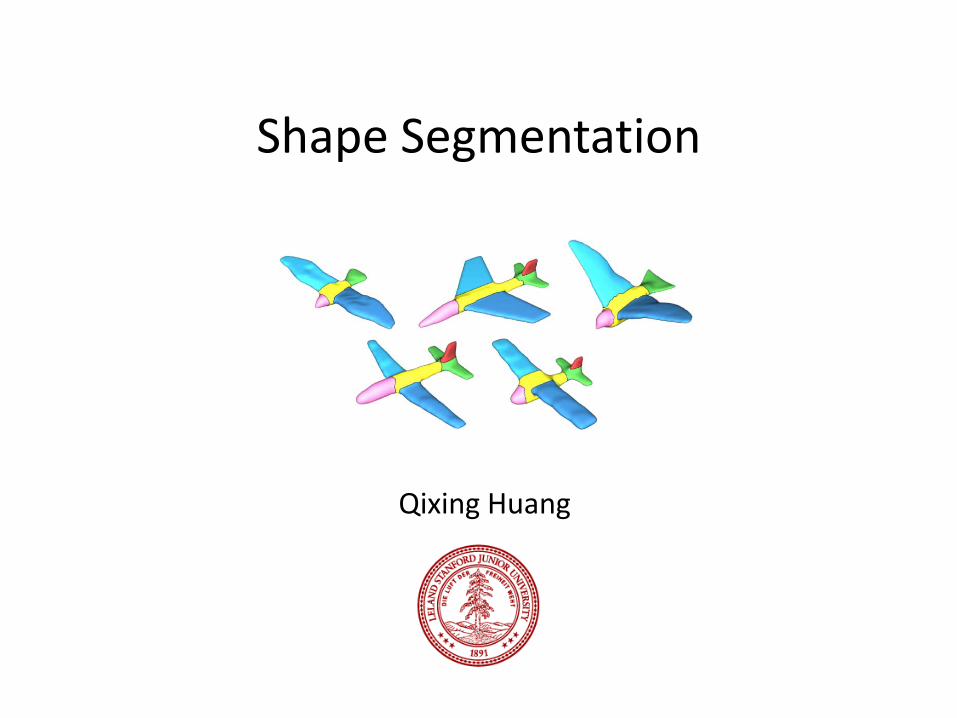
Shape Segmentation
Qixing Huang
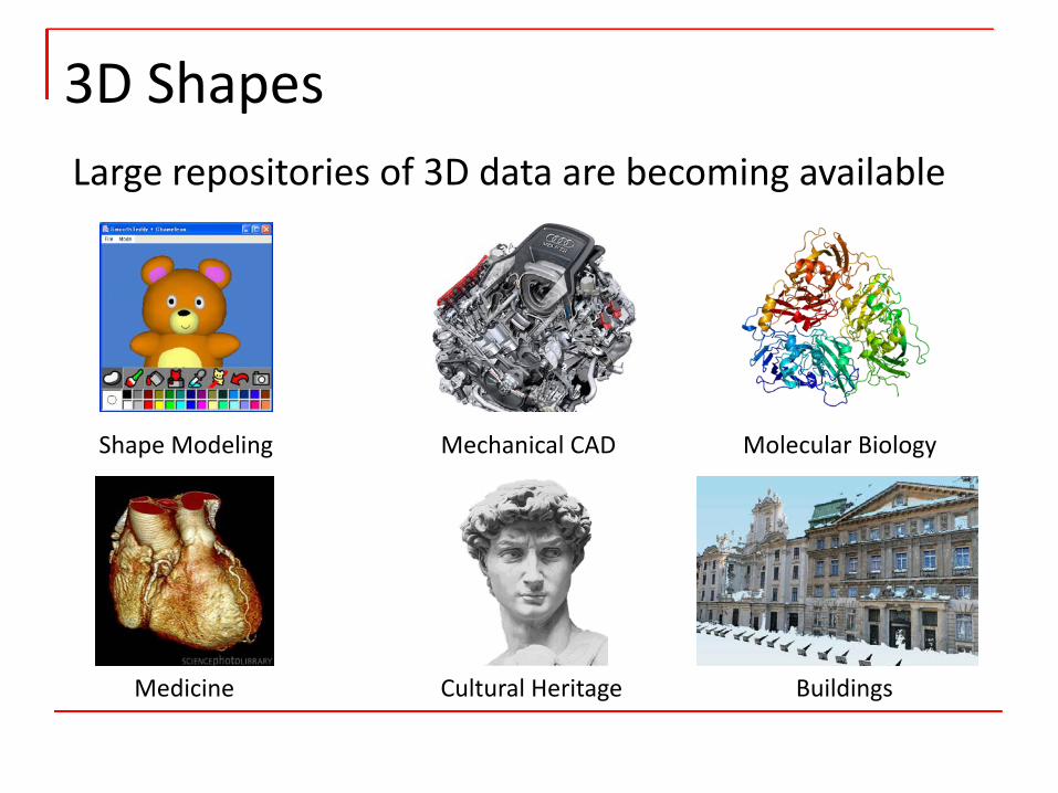
3D Shapes
Shape Modeling Mechanical CAD Molecular Biology
Medicine Cultural Heritage Buildings
Large repositories of 3D data are becoming available
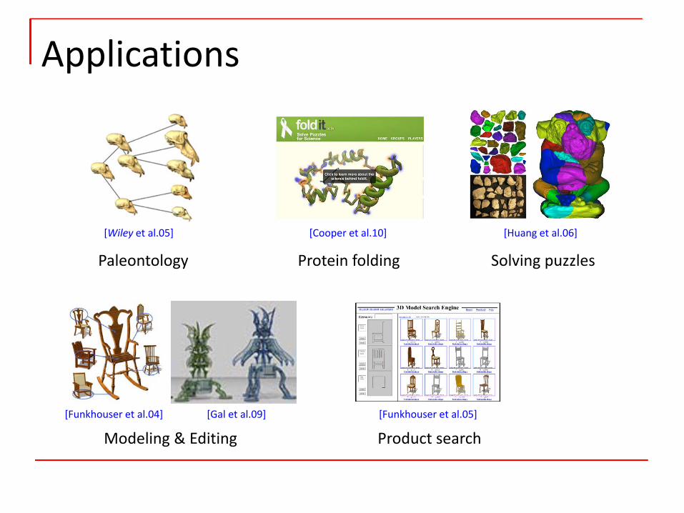
Applications
Modeling & Editing [Gal et al.09][Funkhouser et al.04]
Product search[Funkhouser et al.05]
Solving puzzles
[Huang et al.06]
Paleontology
[Wiley et al.05]
Protein folding
[Cooper et al.10]
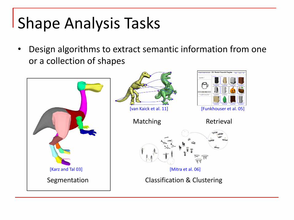
• Design algorithms to extract semantic information from one or a collection of shapes
Shape Analysis Tasks
Segmentation
Matching Retrieval
Classification & Clustering
[van Kaick et al. 11]
[Karz and Tal 03] [Mitra et al. 06]
[Funkhouser et al. 05]
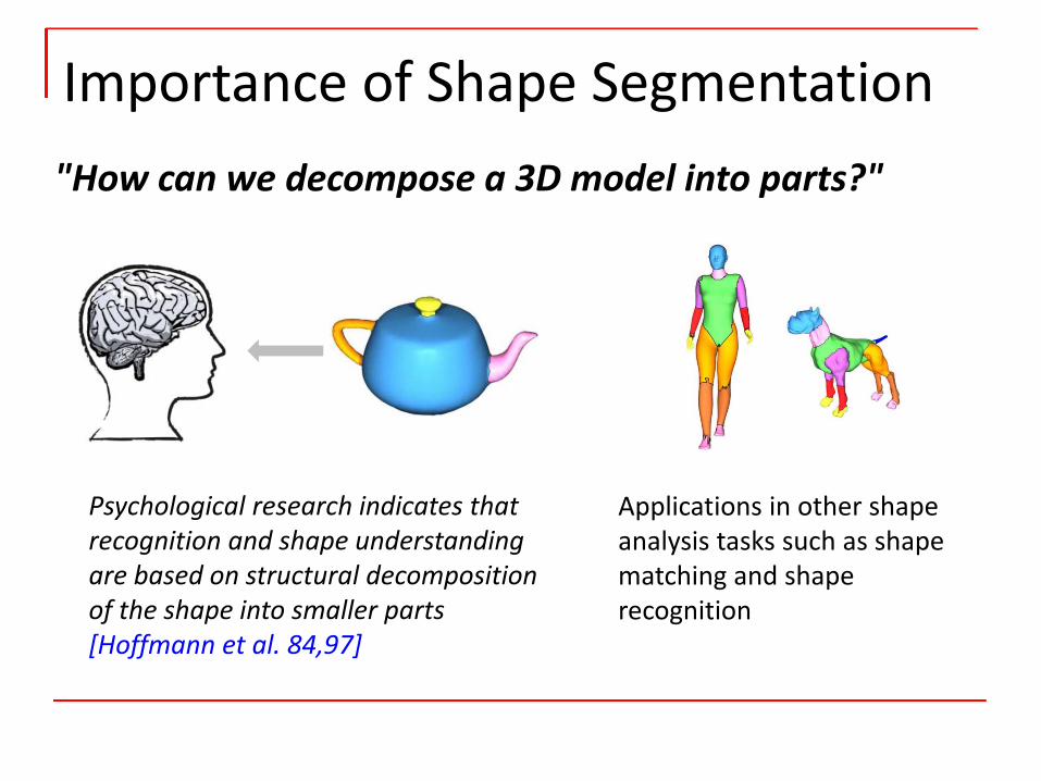
Importance of Shape Segmentation"How can we decompose a 3D model into parts?"
Psychological research indicates that recognition and shape understanding are based on structural decomposition of the shape into smaller parts [Hoffmann et al. 84,97]
Applications in other shape analysis tasks such as shape matching and shape recognition

Outline
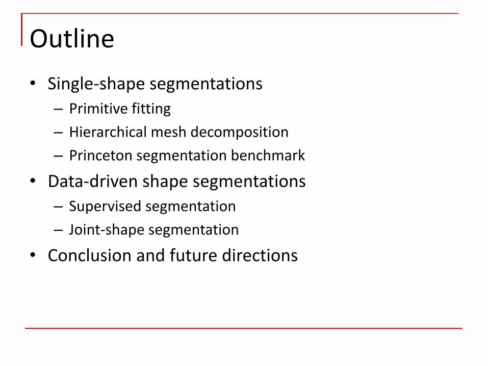
• Single‐shape segmentations– Primitive fitting– Hierarchical mesh decomposition– Princeton segmentation benchmark
• Data‐driven shape segmentations– Supervised segmentation – Joint‐shape segmentation
• Conclusion and future directions
Outline
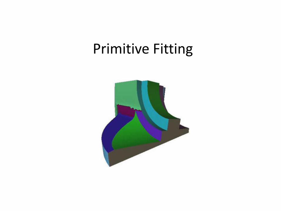
Primitive Fitting
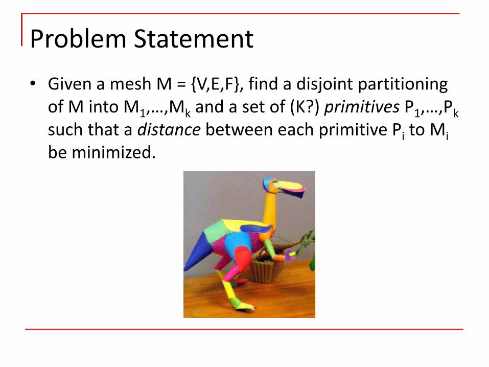
• Given a mesh M = {V,E,F}, find a disjoint partitioning of M into M1,…,Mk and a set of (K?) primitives P1,…,Pksuch that a distance between each primitive Pi to Mibe minimized.
Problem Statement

• Planes or Cylinders
Primitives
[Raab et al. 04][Cohen‐Steiner et al. 04]
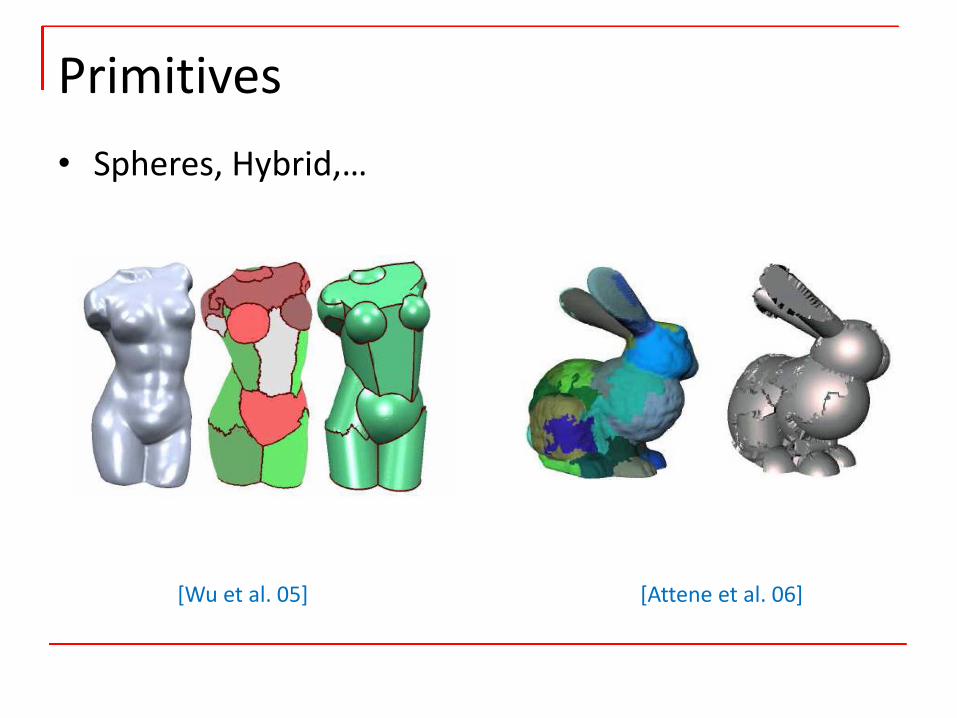
• Spheres, Hybrid,…
Primitives
[Attene et al. 06][Wu et al. 05]
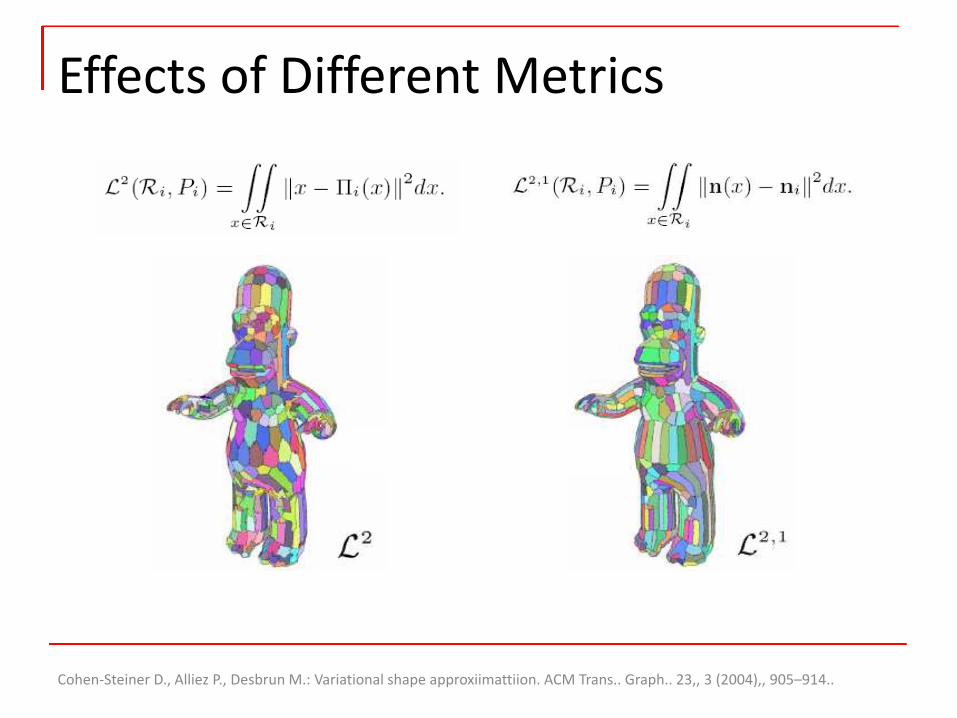
Effects of Different Metrics
Cohen‐Steiner D., Alliez P., Desbrun M.: Variational shape approxiimattiion. ACM Trans.. Graph.. 23,, 3 (2004),, 905–914..
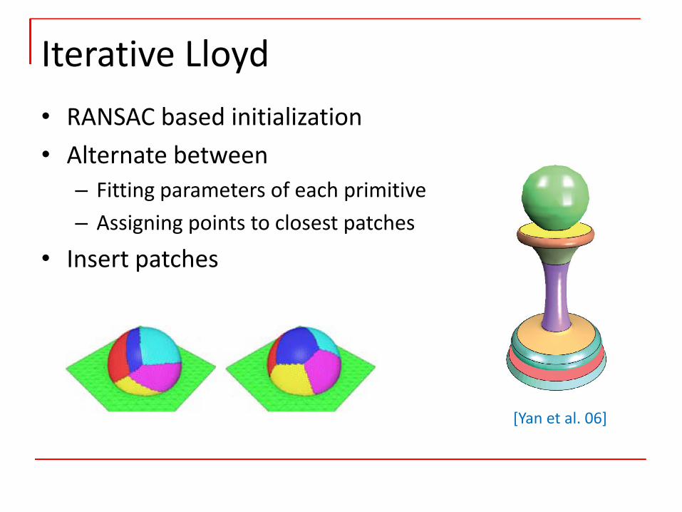
• RANSAC based initialization • Alternate between– Fitting parameters of each primitive– Assigning points to closest patches
• Insert patches
Iterative Lloyd
[Yan et al. 06]
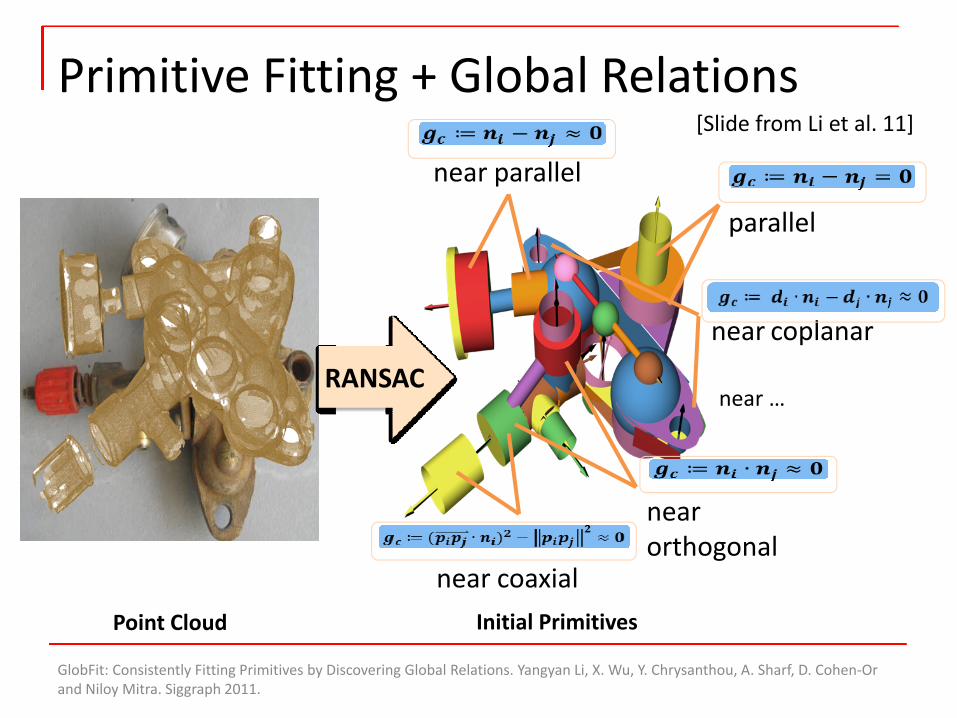
Primitive Fitting + Global Relations
Point Cloud Initial Primitives
parallel
RANSAC
near parallel
near coplanar
near orthogonal
near coaxial
near …
GlobFit: Consistently Fitting Primitives by Discovering Global Relations. Yangyan Li, X. Wu, Y. Chrysanthou, A. Sharf, D. Cohen‐Or and Niloy Mitra. Siggraph 2011.
[Slide from Li et al. 11]
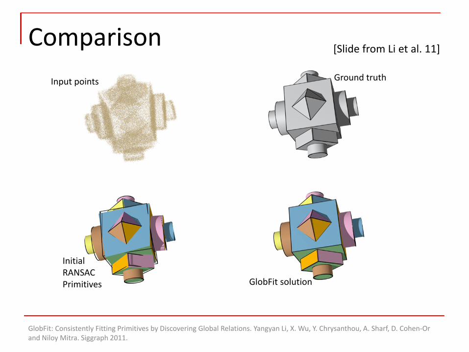
ComparisonGround truthInput points
InitialRANSACPrimitives GlobFit solution
GlobFit: Consistently Fitting Primitives by Discovering Global Relations. Yangyan Li, X. Wu, Y. Chrysanthou, A. Sharf, D. Cohen‐Or and Niloy Mitra. Siggraph 2011.
[Slide from Li et al. 11]
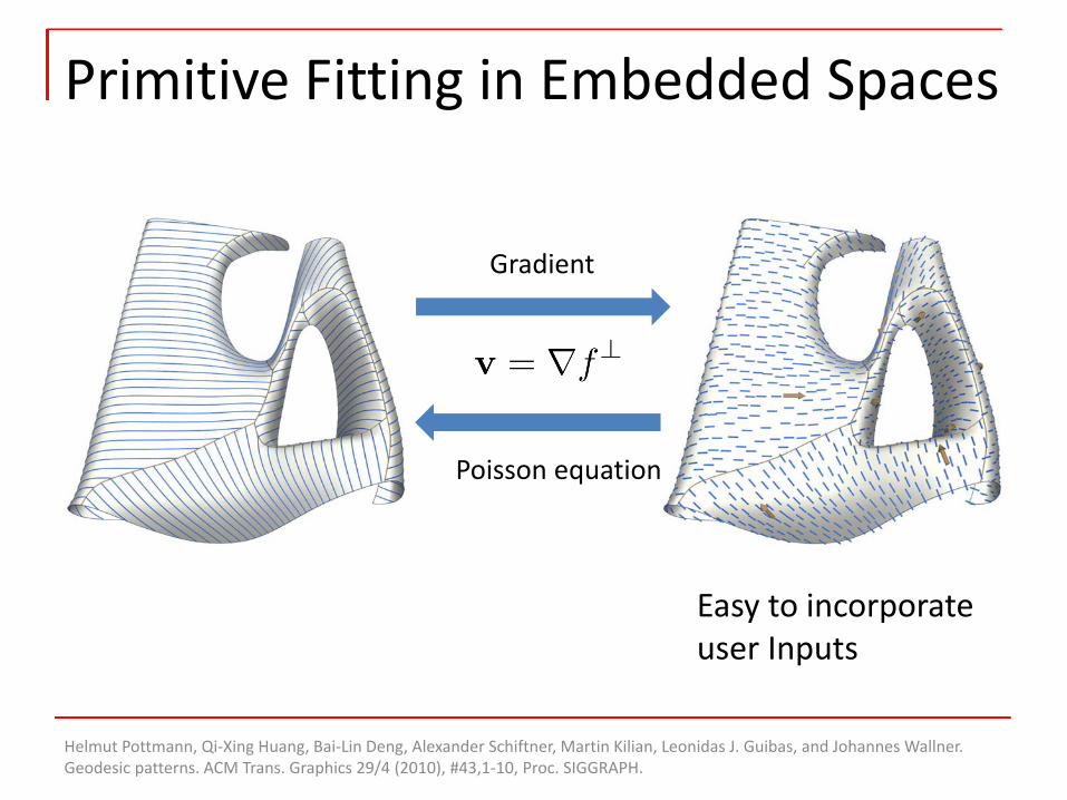
Primitive Fitting in Embedded Spaces
Easy to incorporateuser Inputs
Gradient
Poisson equation
Helmut Pottmann, Qi‐Xing Huang, Bai‐Lin Deng, Alexander Schiftner, Martin Kilian, Leonidas J. Guibas, and Johannes Wallner. Geodesic patterns. ACM Trans. Graphics 29/4 (2010), #43,1‐10, Proc. SIGGRAPH.

Cont‐
• Based on the assumption that patches can approximately described by simple primitives– CAD– Man‐made objects
• Iterative Lloyd for optimization• Advanced primitive fitting– Structural constraints– In embedded space
Primitive Fitting
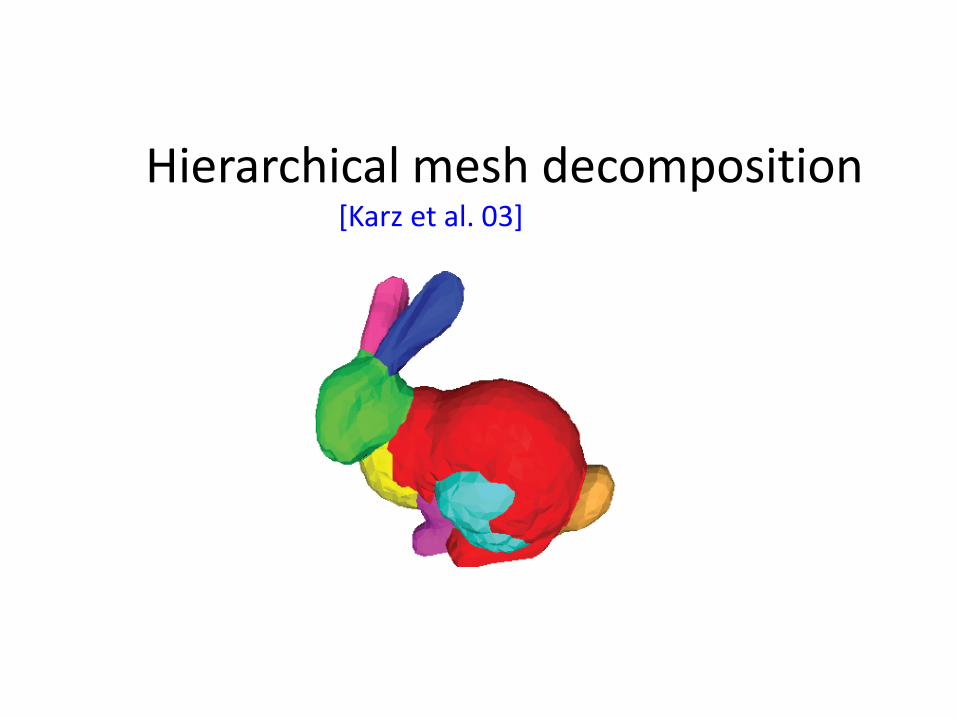
Hierarchical mesh decomposition[Karz et al. 03]
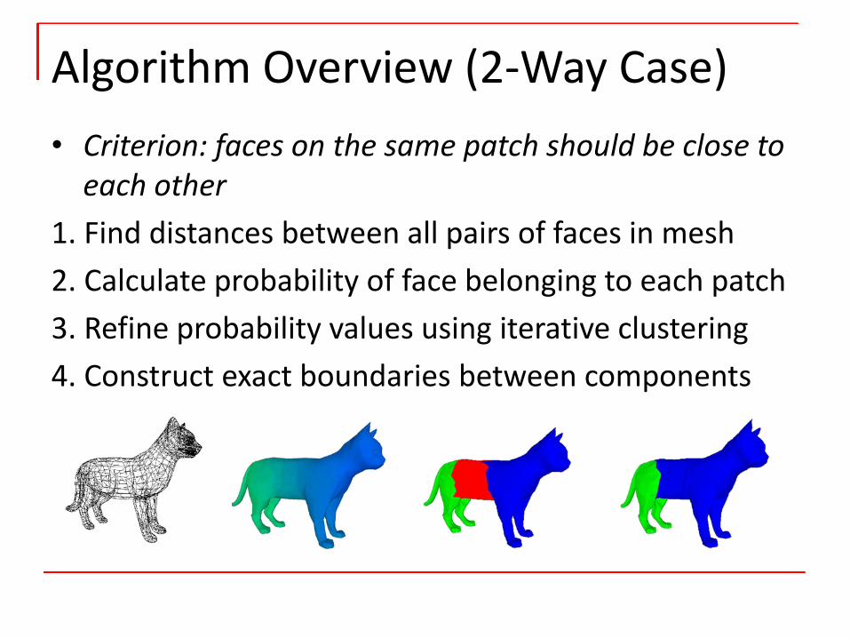
• Criterion: faces on the same patch should be close to each other
1. Find distances between all pairs of faces in mesh2. Calculate probability of face belonging to each patch3. Refine probability values using iterative clustering4. Construct exact boundaries between components
Algorithm Overview (2‐Way Case)
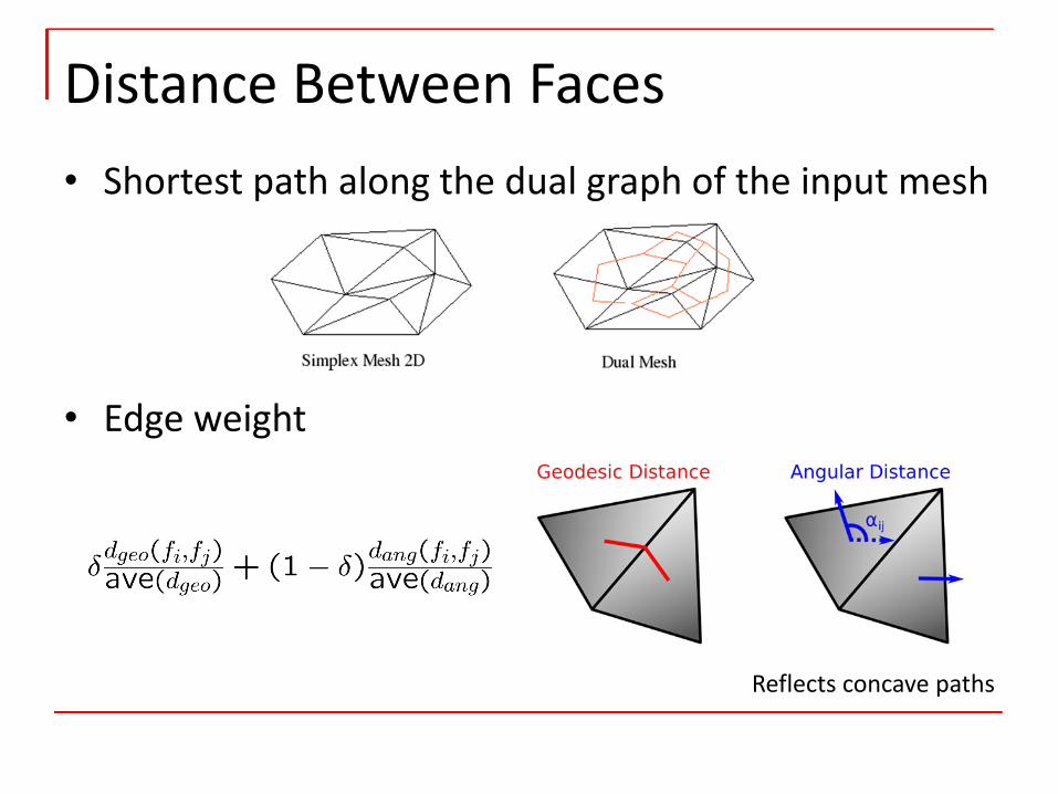
• Shortest path along the dual graph of the input mesh
• Edge weight
Distance Between Faces
Reflects concave paths

• Farthest point sampling– stay far away from existing seeds
Selecting Seed Faces
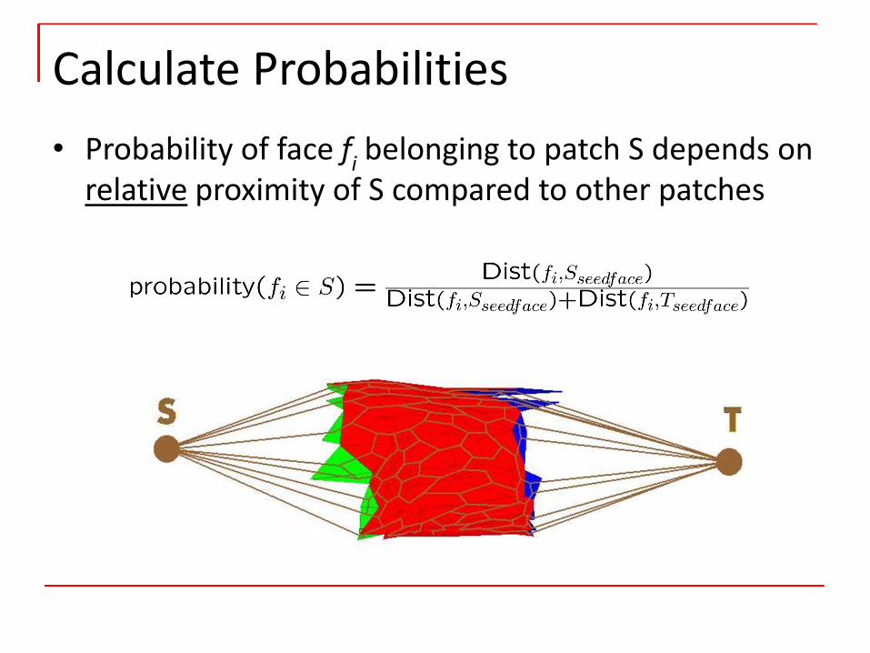
• Probability of face fi belonging to patch S depends on relative proximity of S compared to other patches
Calculate Probabilities
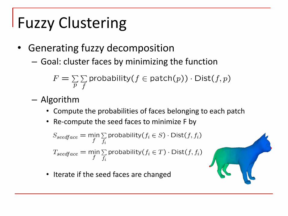
• Generating fuzzy decomposition– Goal: cluster faces by minimizing the function
– Algorithm• Compute the probabilities of faces belonging to each patch• Re‐compute the seed faces to minimize F by
• Iterate if the seed faces are changed
Fuzzy Clustering
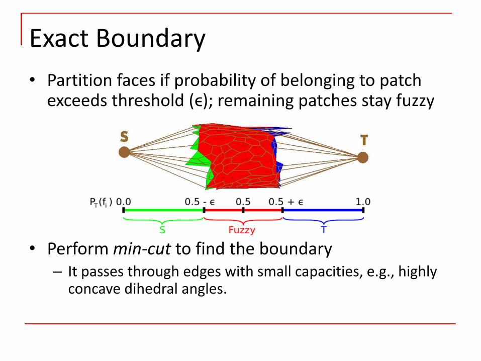
• Partition faces if probability of belonging to patch exceeds threshold (ϵ); remaining patches stay fuzzy
• Perform min‐cut to find the boundary– It passes through edges with small capacities, e.g., highly concave dihedral angles.
Exact Boundary
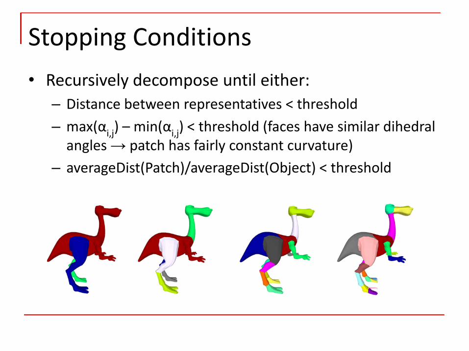
• Recursively decompose until either:– Distance between representatives < threshold– max(αi,j) – min(αi,j) < threshold (faces have similar dihedral angles → patch has fairly constant curvature)
– averageDist(Patch)/averageDist(Object) < threshold
Stopping Conditions
• Represent meshes as dual graphs• Find a meaningful graph distance metric• Points on the same patch are close to each other– Fuzzy clustering
• Min‐cut for extract boundaries
Hierarchical Mesh Decomposition

Other approaches
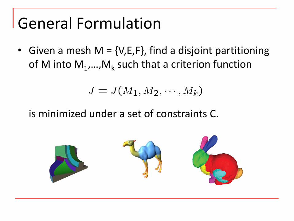
• Given a mesh M = {V,E,F}, find a disjoint partitioning of M into M1,…,Mk such that a criterion function
is minimized under a set of constraints C.
General Formulation
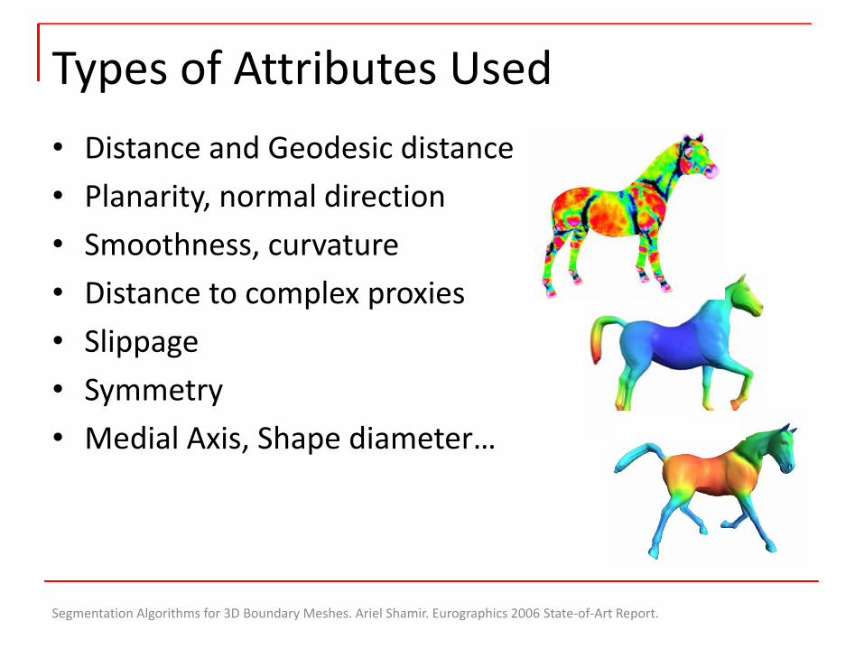
• Distance and Geodesic distance• Planarity, normal direction• Smoothness, curvature• Distance to complex proxies• Slippage• Symmetry• Medial Axis, Shape diameter…
Types of Attributes Used
Segmentation Algorithms for 3D Boundary Meshes. Ariel Shamir. Eurographics 2006 State‐of‐Art Report.
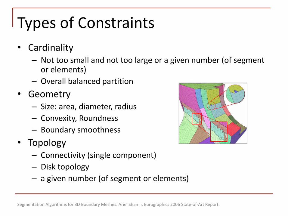
• Cardinality– Not too small and not too large or a given number (of segment
or elements)– Overall balanced partition
• Geometry– Size: area, diameter, radius– Convexity, Roundness– Boundary smoothness
• Topology– Connectivity (single component)– Disk topology– a given number (of segment or elements)
Types of Constraints
Segmentation Algorithms for 3D Boundary Meshes. Ariel Shamir. Eurographics 2006 State‐of‐Art Report.
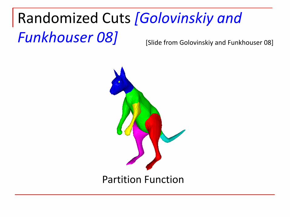
Randomized Cuts [Golovinskiy and Funkhouser 08]
Partition Function
[Slide from Golovinskiy and Funkhouser 08]
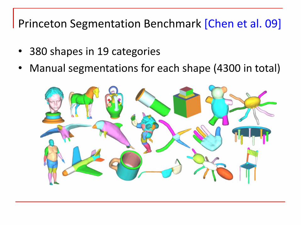
• 380 shapes in 19 categories• Manual segmentations for each shape (4300 in total)
Princeton Segmentation Benchmark [Chen et al. 09]
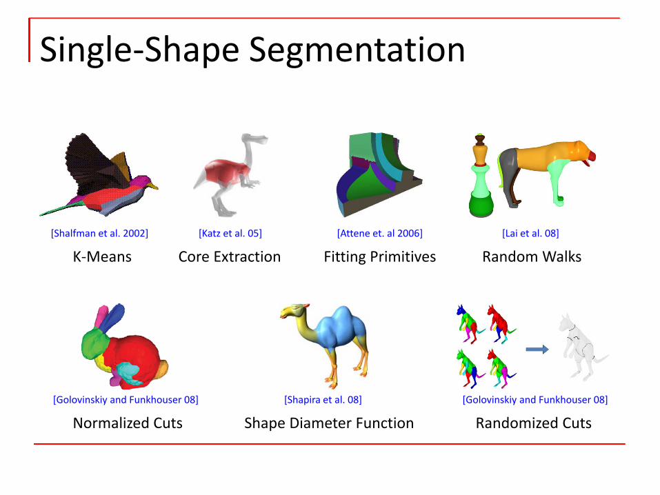
Single‐Shape Segmentation
K‐Means[Shalfman et al. 2002]
Random Walks[Lai et al. 08]
Fitting Primitives[Attene et. al 2006]
Normalized Cuts[Golovinskiy and Funkhouser 08]
Randomized Cuts[Golovinskiy and Funkhouser 08]
Core Extraction[Katz et al. 05]
Shape Diameter Function[Shapira et al. 08]
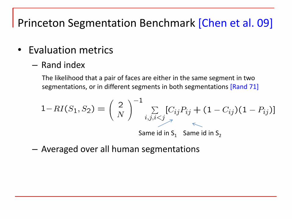
• Evaluation metrics – Rand index
– Averaged over all human segmentations
Princeton Segmentation Benchmark [Chen et al. 09]
The likelihood that a pair of faces are either in the same segment in two segmentations, or in different segments in both segmentations [Rand 71]
Same id in S2Same id in S1
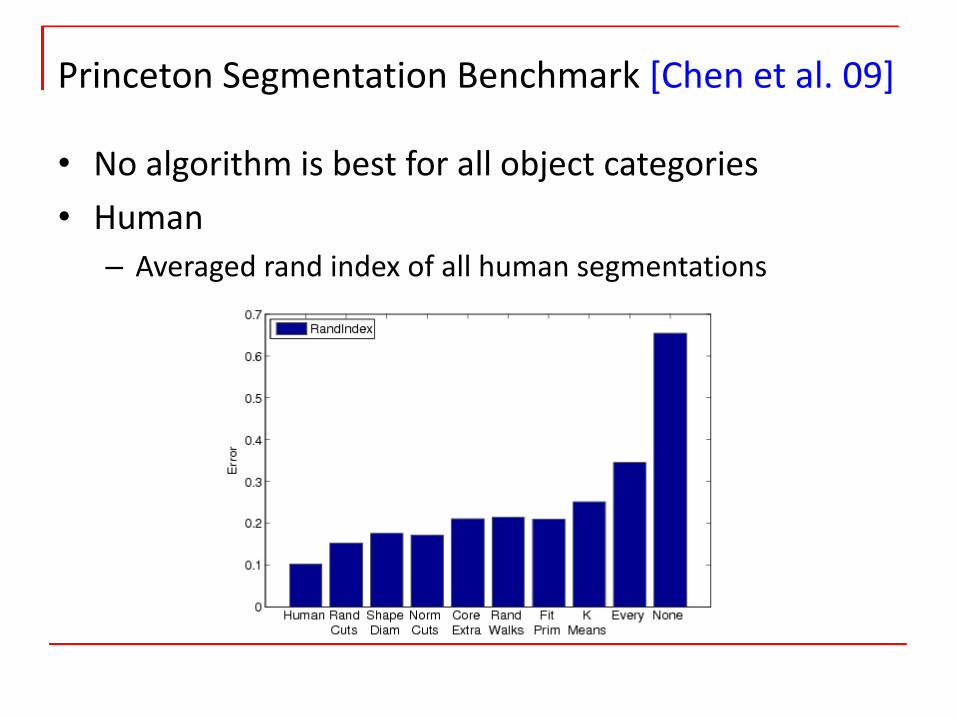
• No algorithm is best for all object categories• Human– Averaged rand index of all human segmentations
Princeton Segmentation Benchmark [Chen et al. 09]
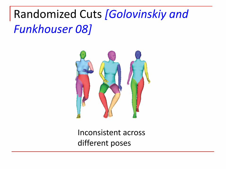
Randomized Cuts [Golovinskiy and Funkhouser 08]
Inconsistent across different poses
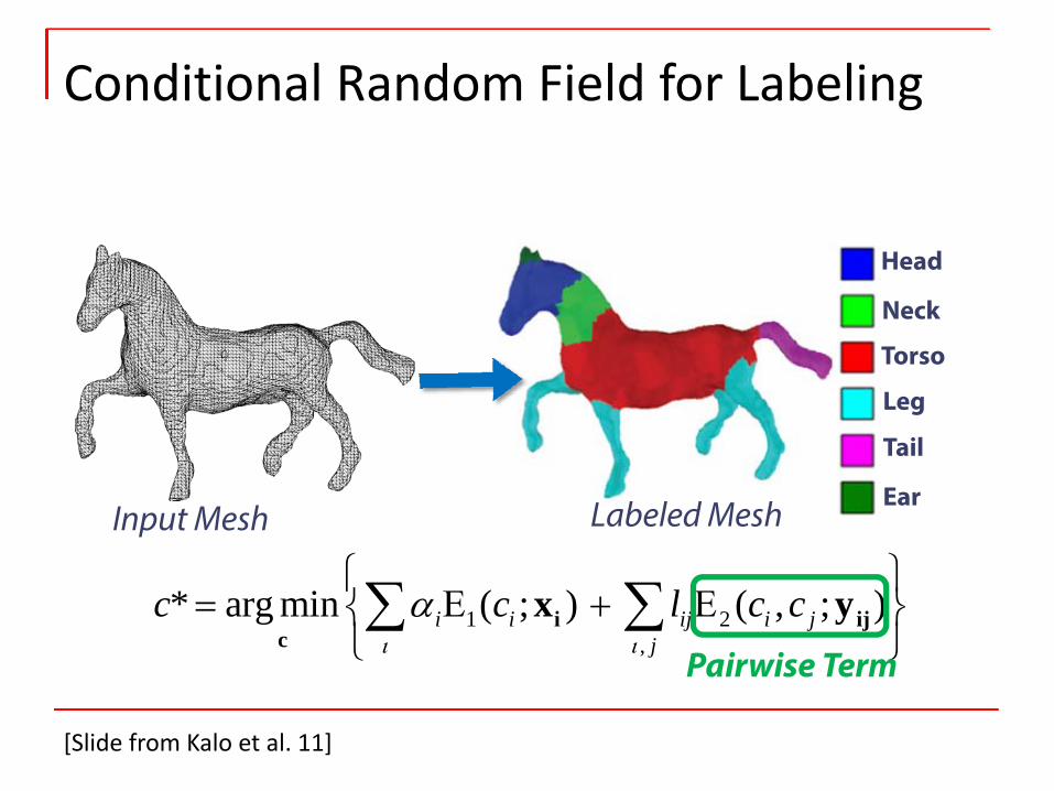
Supervised Segmentation
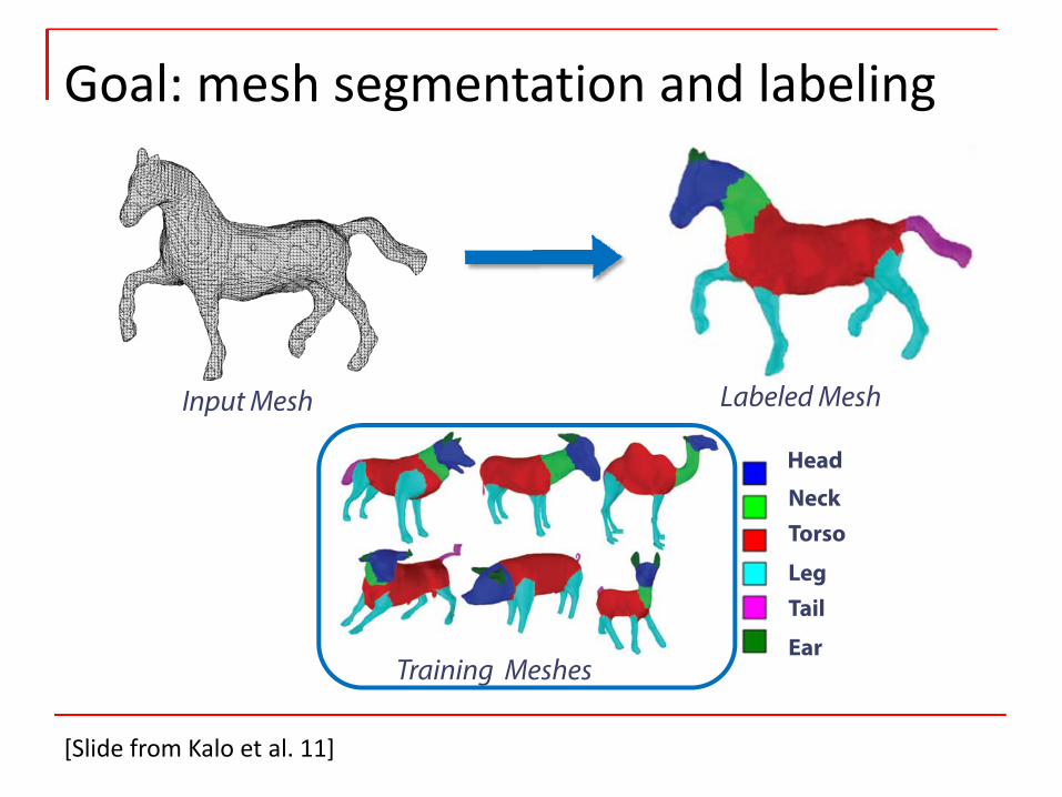
Goal: mesh segmentation and labeling
Input Mesh Labeled Mesh
Training Meshes
Head
NeckTorso
LegTail
Ear
[Slide from Kalo et al. 11]
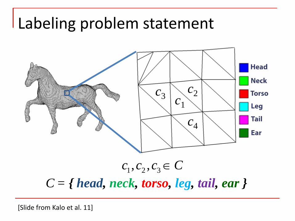
Labeling problem statement
C = { head, neck, torso, leg, tail, ear }
c1
Head
Neck
Torso
Leg
Tail
Ear
c2
c4
c3
1 2 3, , ∈c c c C
[Slide from Kalo et al. 11]
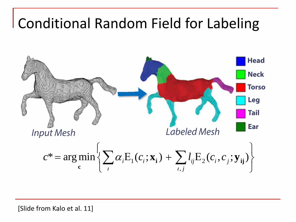
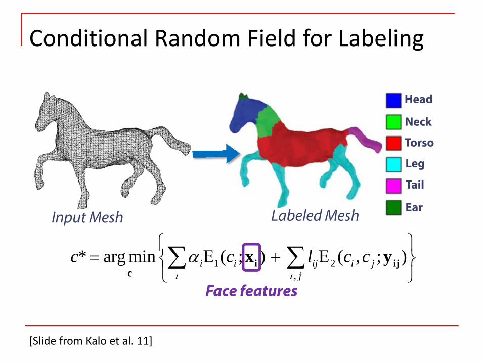
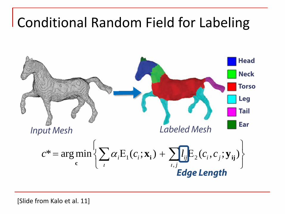
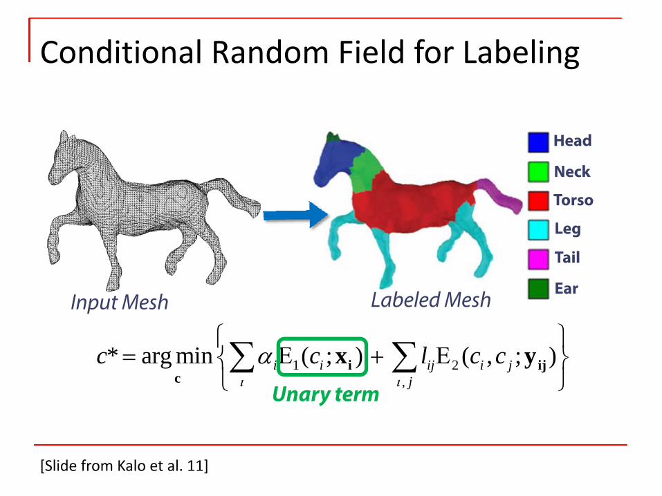
Conditional Random Field for Labeling
1 2,
* arg min ( ; ) ( , ; )i i ij i jj
c c l c cι ι
α⎧ ⎫
= Ε + Ε⎨ ⎬⎩ ⎭∑ ∑i ij
cx y
Input Mesh Labeled Mesh
Head
Neck
Torso
Leg
Tail
Ear
[Slide from Kalo et al. 11]
Conditional Random Field for Labeling
1 2,
* arg min ( ; ) ( , ; )i i ij i jj
c c l c cι ι
α⎧ ⎫
= Ε + Ε⎨ ⎬⎩ ⎭∑ ∑i ij
cx y
Face features
Input Mesh Labeled Mesh
Head
Neck
Torso
Leg
Tail
Ear
[Slide from Kalo et al. 11]
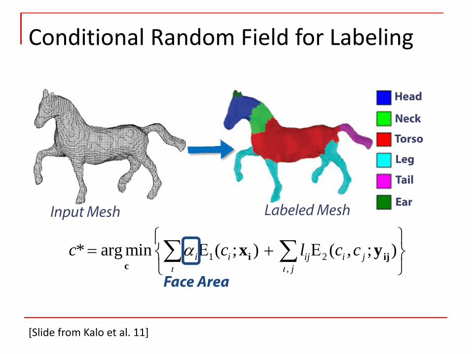
Conditional Random Field for Labeling
1 2,
* arg min ( ; ) ( , ; )i i ij i jj
c c l c cι ι
α⎧ ⎫
= Ε + Ε⎨ ⎬⎩ ⎭∑ ∑i ij
cx y
Face Area
Input Mesh Labeled Mesh
Head
Neck
Torso
Leg
Tail
Ear
[Slide from Kalo et al. 11]
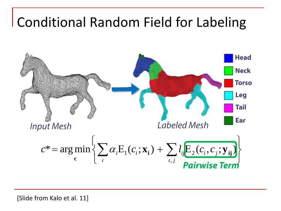
Conditional Random Field for Labeling
1 2,
* arg min ( ; ) ( , ; )i i ij i jj
c c l c cι ι
α⎧ ⎫
= Ε + Ε⎨ ⎬⎩ ⎭∑ ∑i ij
cx y
Pairwise Term
Input Mesh Labeled Mesh
Head
Neck
Torso
Leg
Tail
Ear
[Slide from Kalo et al. 11]
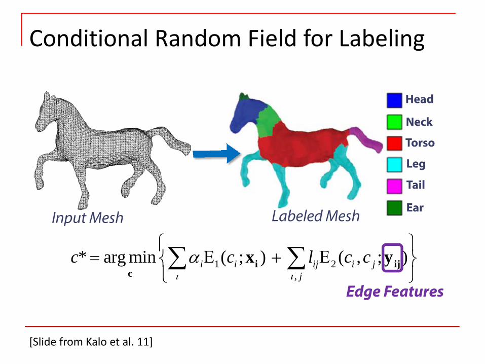
Conditional Random Field for Labeling
1 2,
* arg min ( ; ) ( , ; )i i ij i jj
c c l c cι ι
α⎧ ⎫
= Ε + Ε⎨ ⎬⎩ ⎭∑ ∑i ij
cx y
Edge Features
Input Mesh Labeled Mesh
Head
Neck
Torso
Leg
Tail
Ear
[Slide from Kalo et al. 11]
Conditional Random Field for Labeling
1 2,
* arg min ( ; ) ( , ; )i i ij i jj
c c l c cι ι
α⎧ ⎫
= Ε + Ε⎨ ⎬⎩ ⎭∑ ∑i ij
cx y
Edge Length
Input Mesh Labeled Mesh
Head
Neck
Torso
Leg
Tail
Ear
[Slide from Kalo et al. 11]
Conditional Random Field for Labeling
1 2,
* arg min ( ; ) ( , ; )i i ij i jj
c c l c cι ι
α⎧ ⎫
= Ε + Ε⎨ ⎬⎩ ⎭∑ ∑i ij
cx y
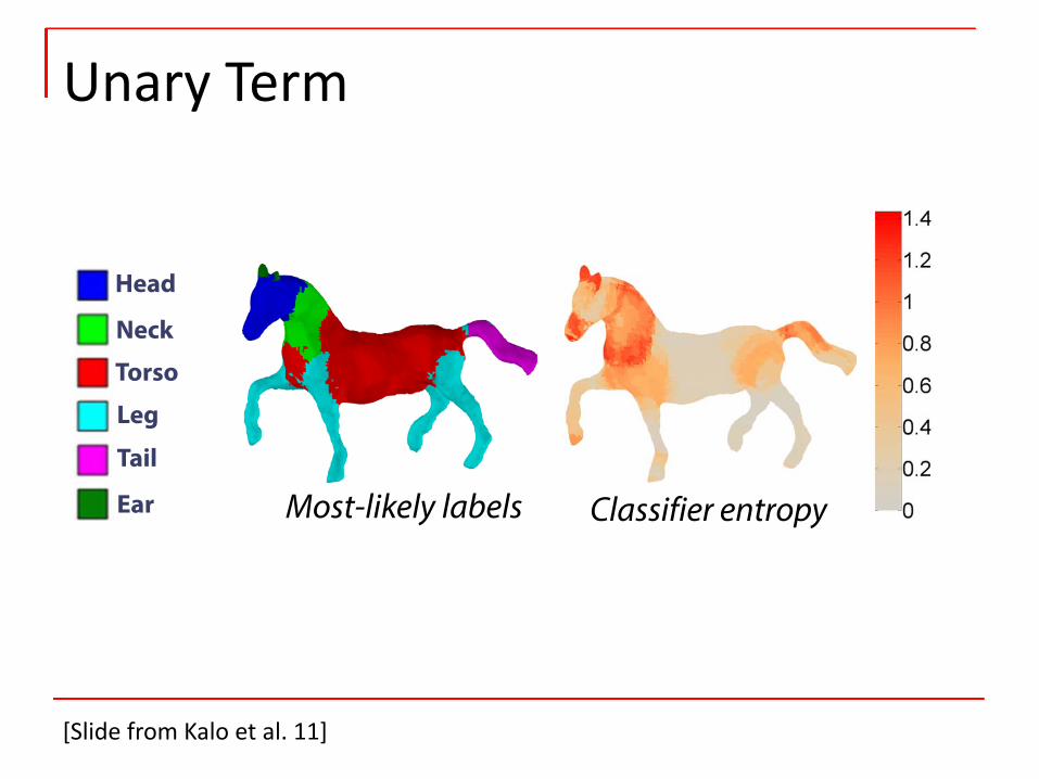
Unary term
Input Mesh Labeled Mesh
Head
Neck
Torso
Leg
Tail
Ear
[Slide from Kalo et al. 11]
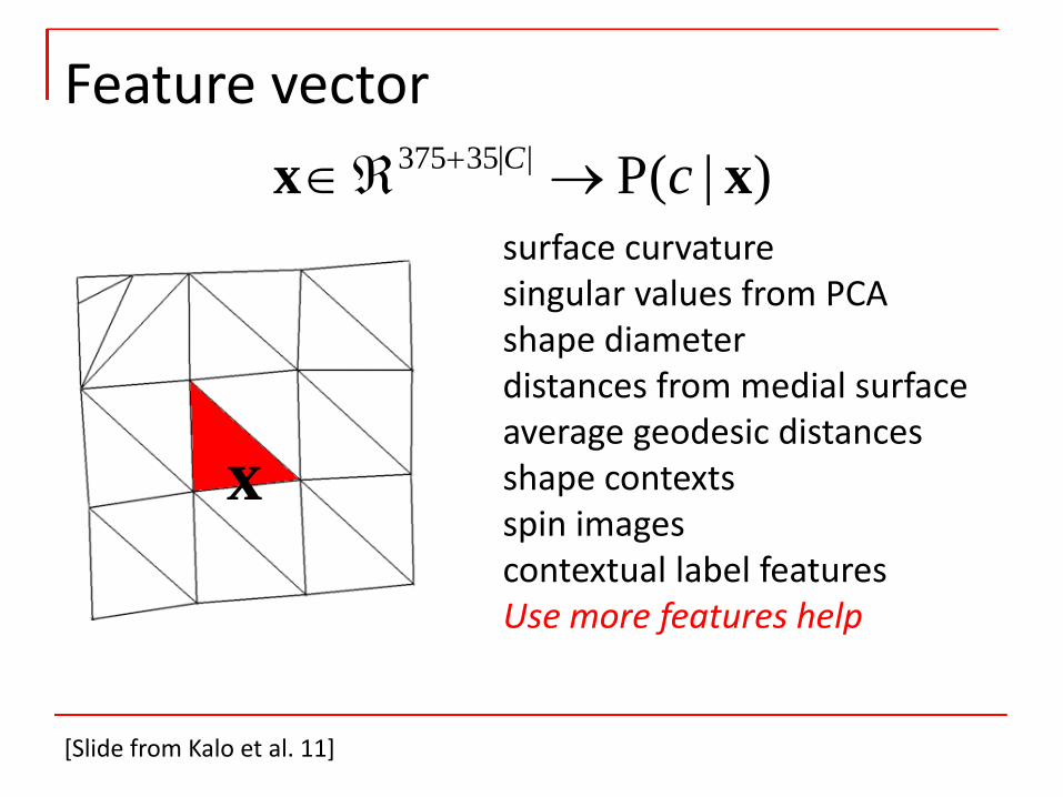
Feature vector
x
surface curvaturesingular values from PCAshape diameter distances from medial surfaceaverage geodesic distancesshape contextsspin imagescontextual label featuresUse more features help
375 35| | P( | )+∈ℜ →C cx x
[Slide from Kalo et al. 11]
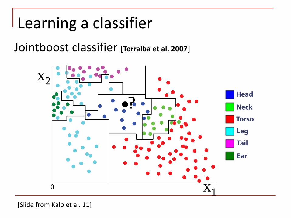
Learning a classifier
x2
x1
Head
Neck
Torso
Leg
Tail
Ear
?
Jointboost classifier [Torralba et al. 2007]
[Slide from Kalo et al. 11]
Unary Term
Most-likely labels
arg max ( | )c
P c x
Classifier entropy
( | ) log ( | )−∑c
P c P cx x
Head
Neck
Torso
Leg
Tail
Ear
[Slide from Kalo et al. 11]
1 2,
* arg min ( ; ) ( , ; )i i ij i jj
c c l c cι ι
α⎧ ⎫
= Ε + Ε⎨ ⎬⎩ ⎭∑ ∑i ij
cx y
Pairwise Term
Input Mesh Labeled Mesh
Head
Neck
Torso
Leg
Tail
Ear
Conditional Random Field for Labeling
[Slide from Kalo et al. 11]
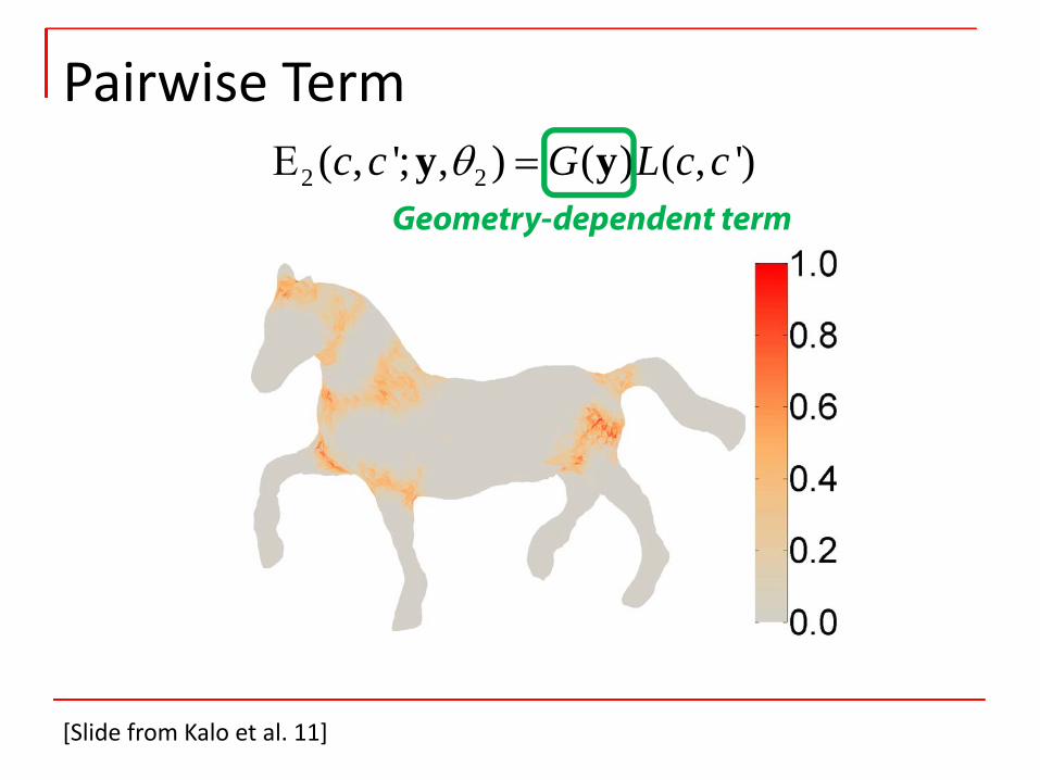
Pairwise Term
Geometry-dependent term2 2( , '; , ) ( ) ( , ')c c G L c cθΕ =y y
[Slide from Kalo et al. 11]
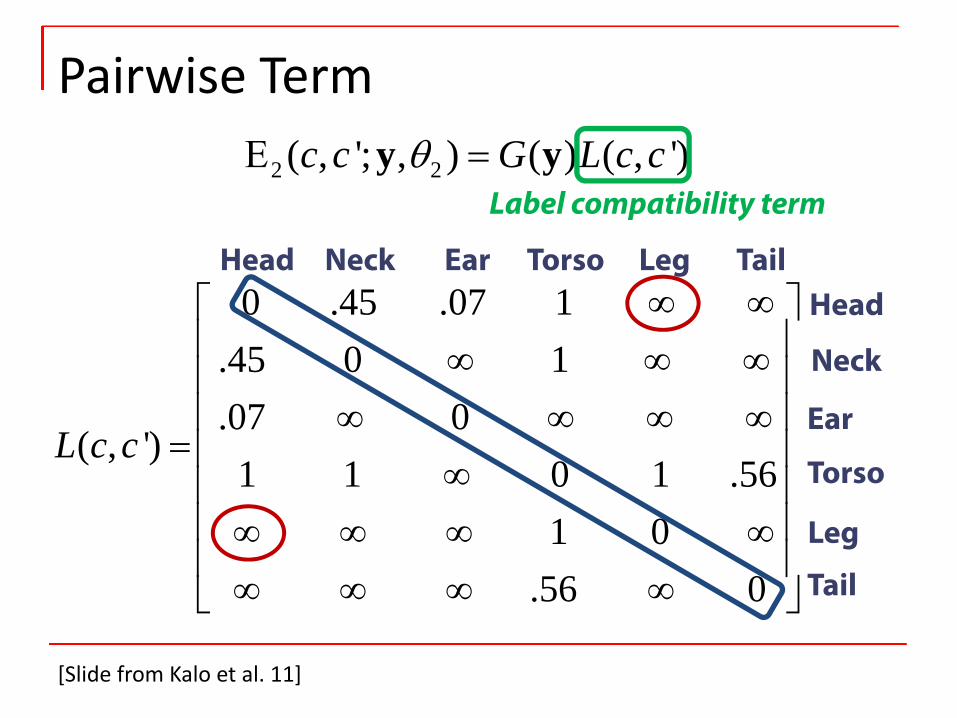
2 2( , '; , ) ( ) ( , ')c c G L c cθΕ =y y
Pairwise Term
Label compatibility term
0 .45 .07 1.45 0 1.07 0
( , ')1 1 0 1 .56
1 0.56 0
L c c
∞ ∞⎡ ⎤⎢ ⎥∞ ∞ ∞⎢ ⎥⎢ ⎥∞ ∞ ∞ ∞
= ⎢ ⎥∞⎢ ⎥⎢ ⎥∞ ∞ ∞ ∞⎢ ⎥∞ ∞ ∞ ∞⎣ ⎦
Head Neck Ear Torso Leg TailHead
Neck
Ear
Torso
Leg
Tail
[Slide from Kalo et al. 11]
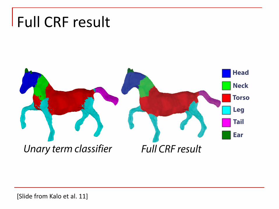
Full CRF result
Head
Neck
Torso
Leg
Tail
Ear
Unary term classifier Full CRF result
[Slide from Kalo et al. 11]
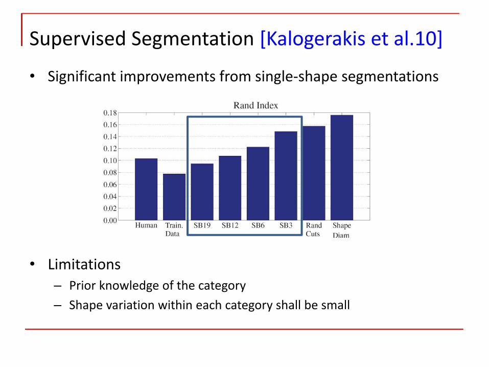
• Significant improvements from single‐shape segmentations
• Limitations– Prior knowledge of the category– Shape variation within each category shall be small
Supervised Segmentation [Kalogerakis et al.10]
Joint Shape Segmentation
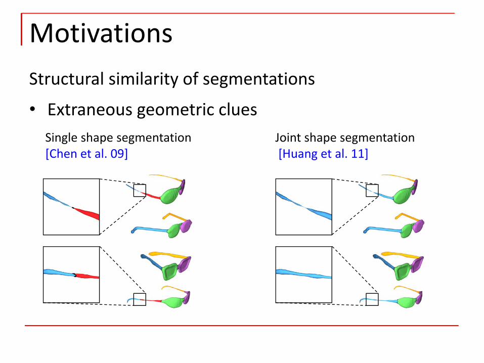
• Extraneous geometric clues
Structural similarity of segmentations
Motivations
Single shape segmentation[Chen et al. 09]
Joint shape segmentation[Huang et al. 11]
Joint shape segmentation[Huang et al. 11]
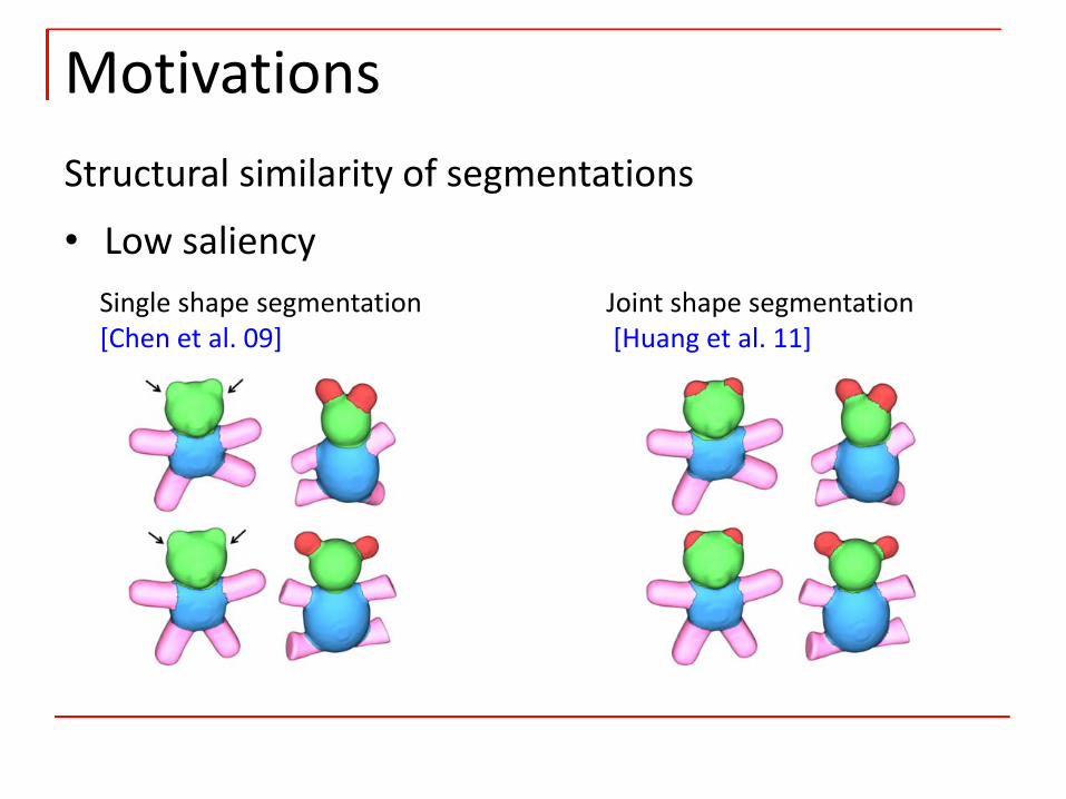
Structural similarity of segmentations
• Low saliency
Motivations
Single shape segmentation[Chen et al. 09]

• Articulated structures
Motivations
Joint shape segmentation[Huang et al. 11]
(Rigid) invariance of segments
Single shape segmentation[Chen et al. 09]
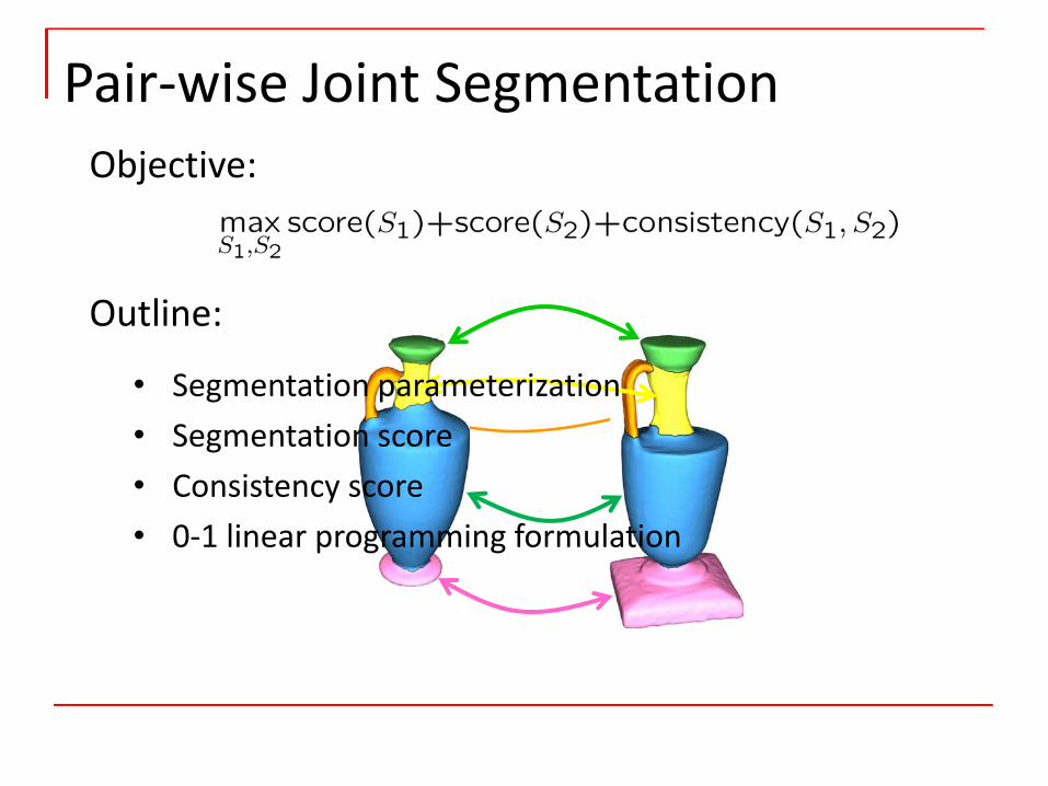
• Segmentation parameterization• Segmentation score• Consistency score • 0‐1 linear programming formulation
Pair‐wise Joint SegmentationObjective:
Outline:
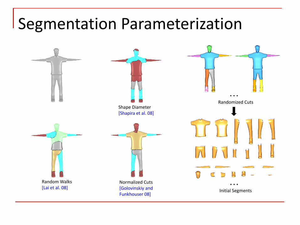
Segmentation Parameterization
Shape Diameter[Shapira et al. 08]
Random Walks[Lai et al. 08]
Normalized Cuts[Golovinskiy and Funkhouser 08]
Randomized Cuts
Initial Segments
Initial Segments
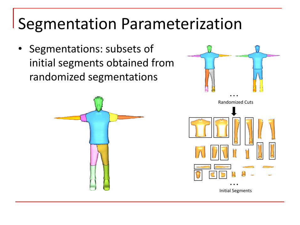
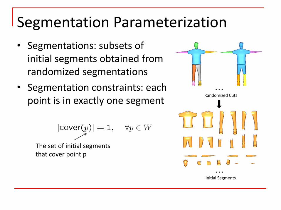
• Segmentations: subsets of initial segments obtained from randomized segmentations
Segmentation Parameterization
Randomized Cuts
• Segmentations: subsets of initial segments obtained from randomized segmentations
• Segmentation constraints: each point is in exactly one segment
Segmentation Parameterization
The set of initial segments that cover point p
Randomized Cuts
Initial Segments
• Segmentations: subsets of initial segments obtained from randomized segmentations
• Segmentation constraints: each point is in exactly one segment
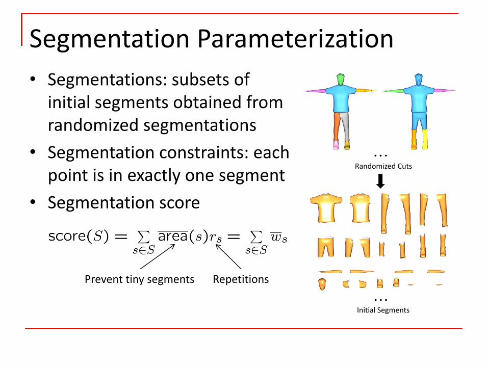
• Segmentation score
Segmentation Parameterization
Prevent tiny segments Repetitions
Randomized Cuts
Initial Segments
Segmentation Parameterization
Randomized Cuts
Initial Segments
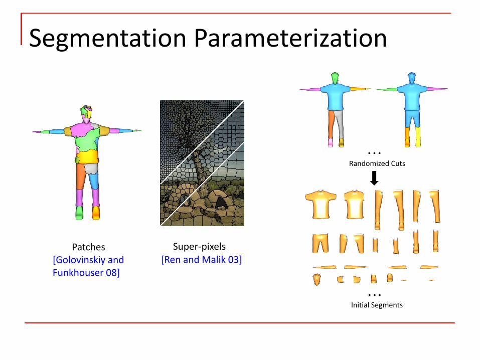
Super‐pixels[Ren and Malik 03]
Patches[Golovinskiy and Funkhouser 08]
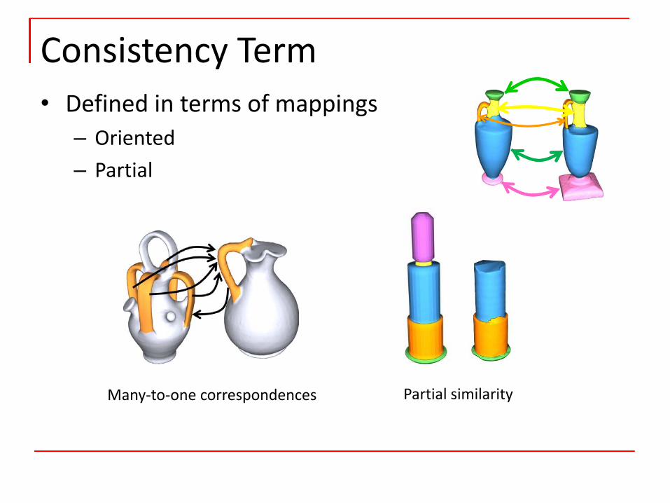
• Defined in terms of mappings– Oriented– Partial
Consistency Term
Many‐to‐one correspondences Partial similarity
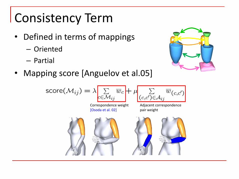
• Defined in terms of mappings– Oriented– Partial
• Mapping score [Anguelov et al.05]
Consistency Term
Correspondence weight [Osoda et al. 02]
Adjacent correspondence pair weight
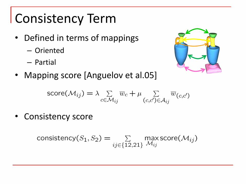
• Defined in terms of mappings– Oriented– Partial
• Mapping score [Anguelov et al.05]
• Consistency score
Consistency Term
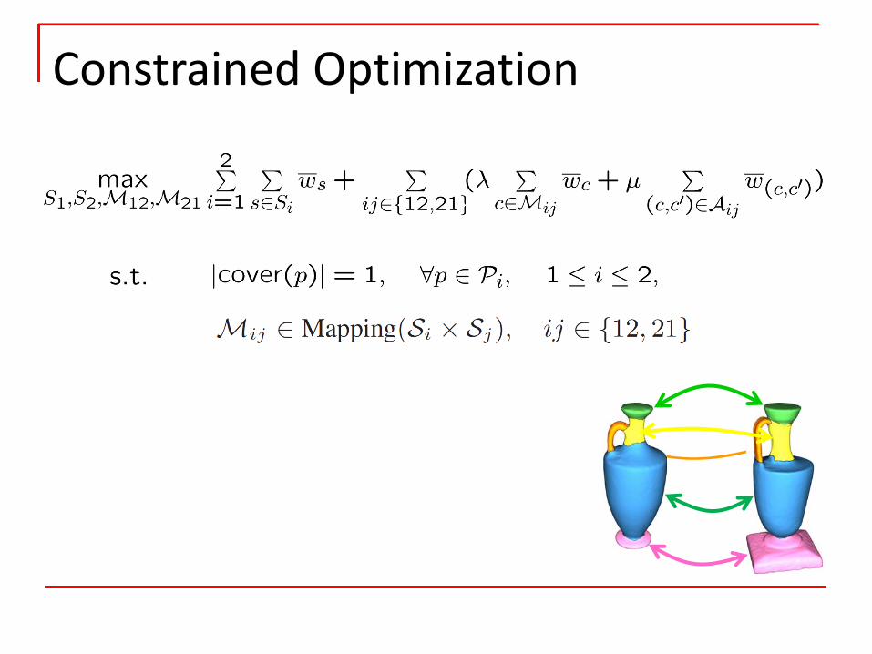
Constrained Optimization
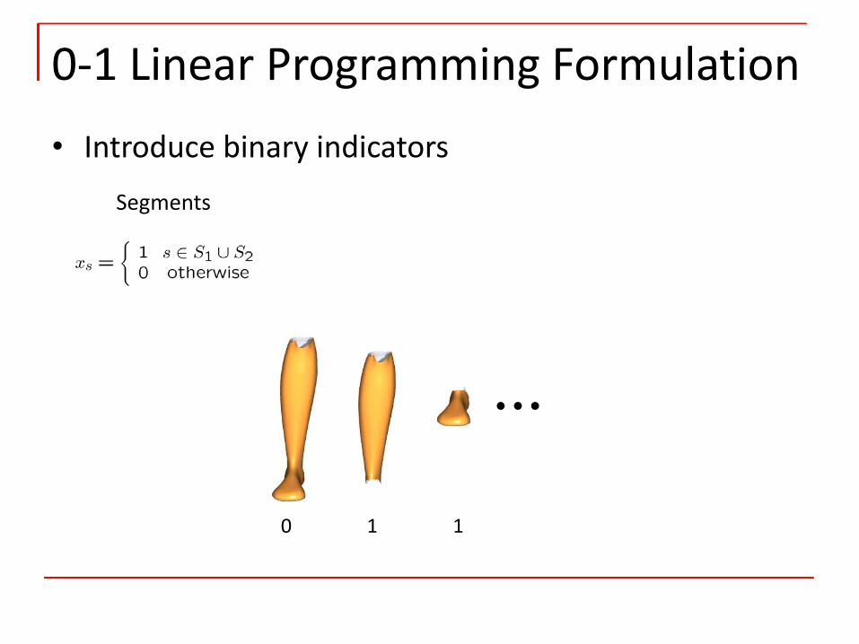
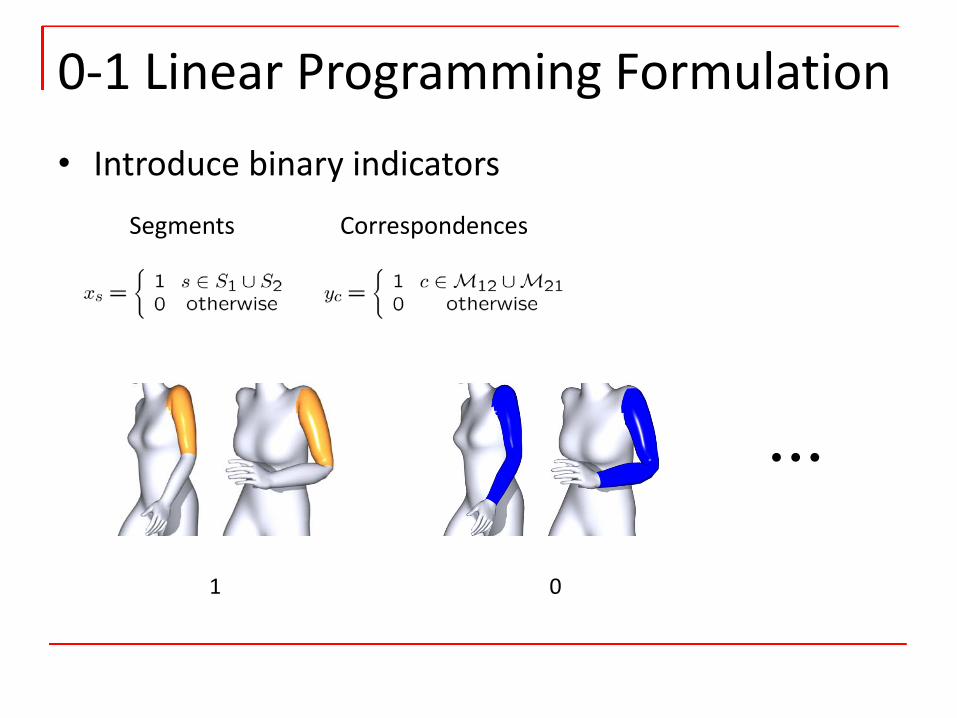
• Introduce binary indicators
0‐1 Linear Programming Formulation
Segments
0 1 1
• Introduce binary indicators
0‐1 Linear Programming Formulation
Segments Correspondences
1 0
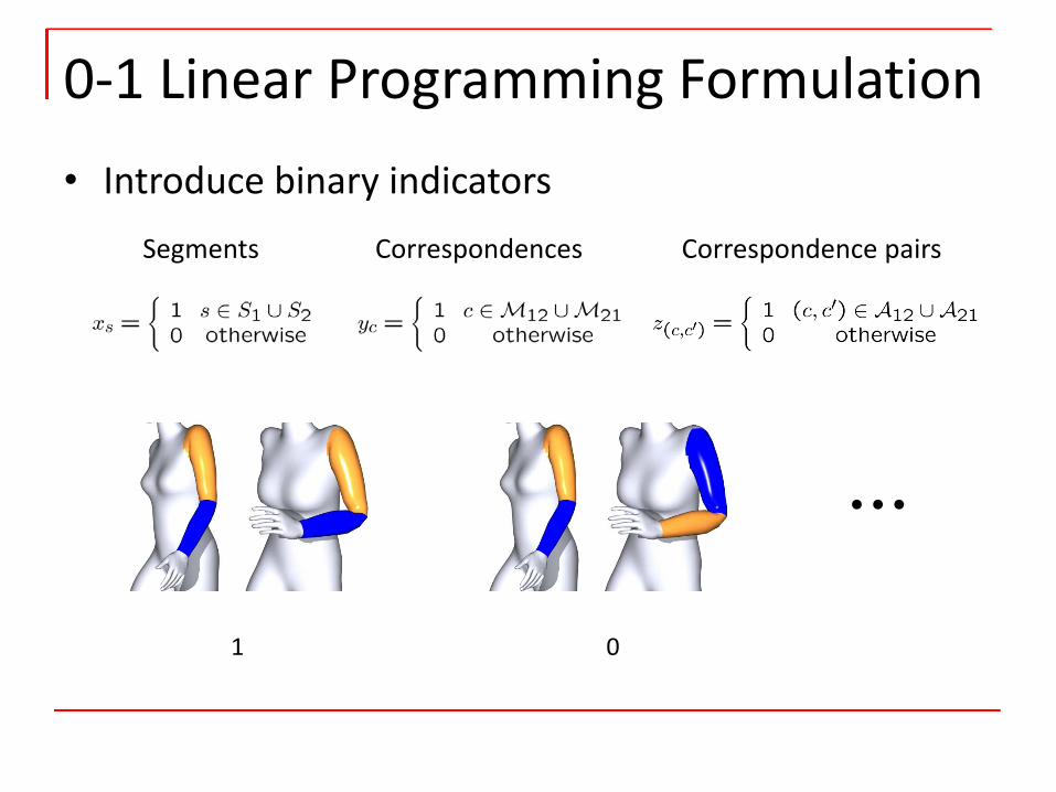
• Introduce binary indicators
0‐1 Linear Programming Formulation
Segments Correspondences Correspondence pairs
1 0
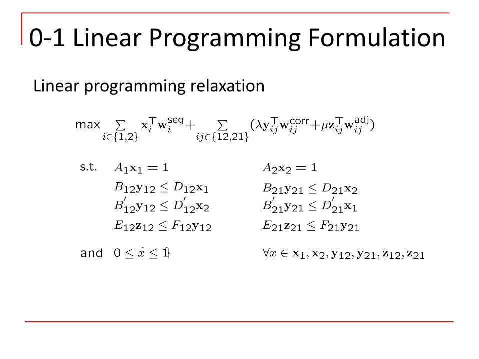
0‐1 Linear Programming Formulation
Linear programming relaxation
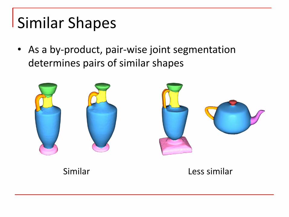
Similar Shapes
Similar Less similar
• As a by‐product, pair‐wise joint segmentation determines pairs of similar shapes
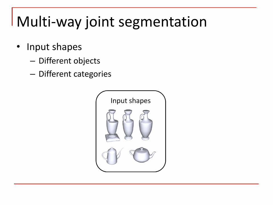
• Input shapes– Different objects– Different categories
Multi‐way joint segmentation
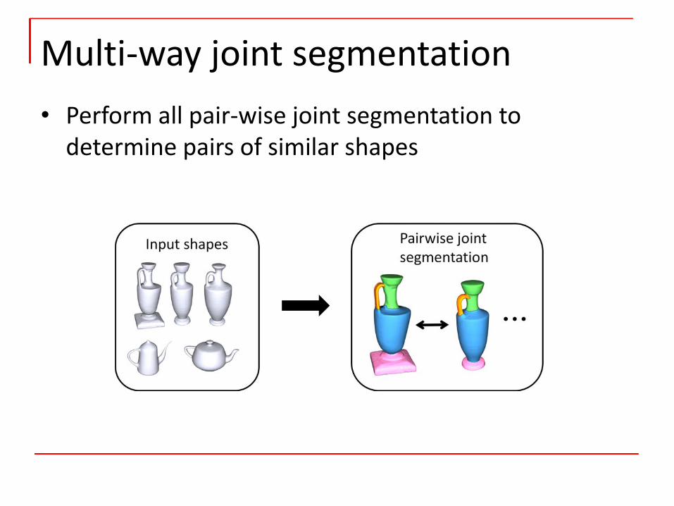
• Perform all pair‐wise joint segmentation to determine pairs of similar shapes
Multi‐way joint segmentation

• Objective function
Multi‐way joint segmentation
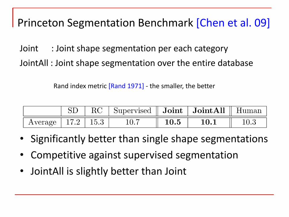
Princeton Segmentation Benchmark [Chen et al. 09]
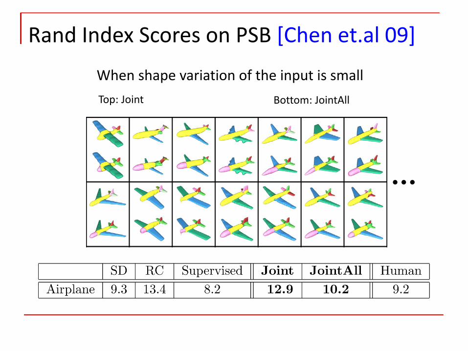
• Significantly better than single shape segmentations• Competitive against supervised segmentation• JointAll is slightly better than Joint
Joint : Joint shape segmentation per each categoryJointAll : Joint shape segmentation over the entire database
Rand index metric [Rand 1971] ‐ the smaller, the better
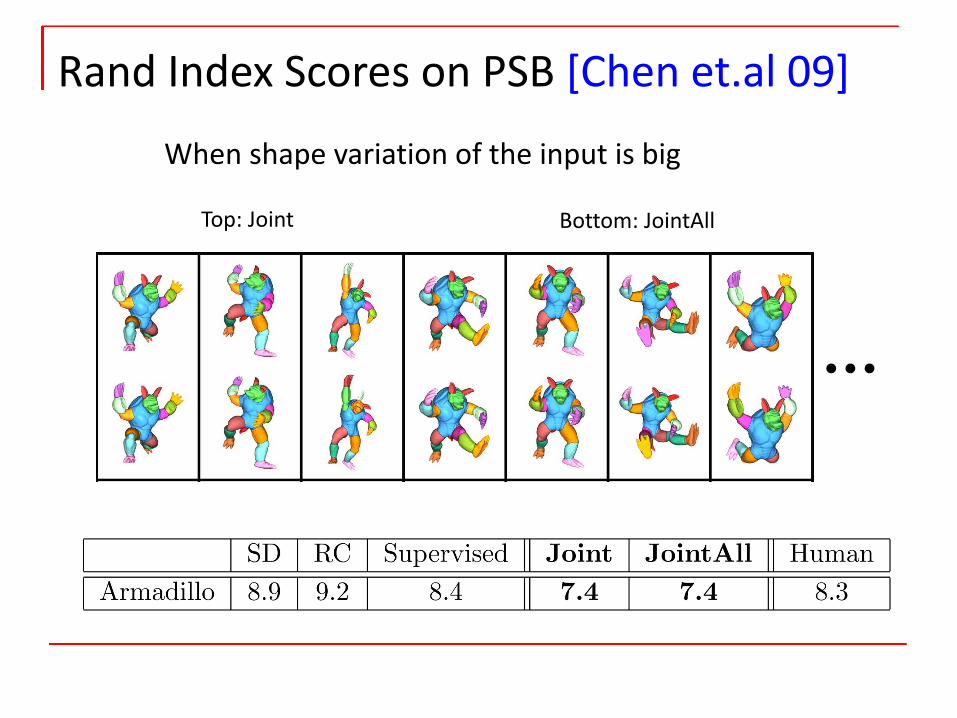
Rand Index Scores on PSB [Chen et.al 09]
When shape variation of the input is big
Top: Joint Bottom: JointAll
Rand Index Scores on PSB [Chen et.al 09]
Top: Joint Bottom: JointAll
When shape variation of the input is small
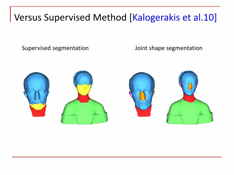
Versus Supervised Method [Kalogerakis et al.10]
Supervised segmentation Joint shape segmentation
• Single‐shape segmentations are limited– No algorithm is suitable for any shape categories
• Data‐driven shape segmentations can improve segmentation quality
• The behavior of supervised method and unsupervised method is different– Supervised method requires shapes to be similar to each other
– Unsupervised method requires variation in shapes
Summary
• Hierarchical segmentation• Man‐made objects
Future directions
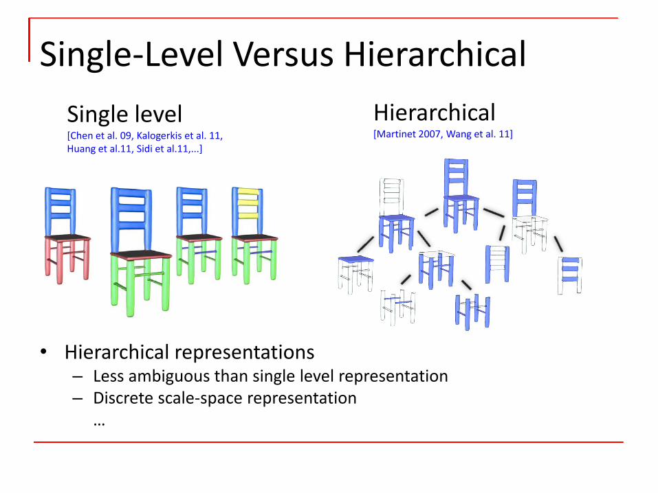
Single‐Level Versus HierarchicalSingle level [Chen et al. 09, Kalogerkis et al. 11,Huang et al.11, Sidi et al.11,...]
Hierarchical[Martinet 2007, Wang et al. 11]
• Hierarchical representations– Less ambiguous than single level representation– Discrete scale‐space representation
…

Architectural Models